Thermalization propagation front and robustness against avalanches in localized systems

Abstract

We investigate the robustness of the many-body localized (MBL) phase to the quantum-avalanche instability by studying the dynamics of a localized spin chain coupled to a $T=\infty$ thermal bath through its leftmost site. By analyzing local magnetizations and quantum mutual information, we estimate the size of the thermalized sector of the chain and find that it increases logarithmically slowly in time. This logarithmically slow propagation of the thermalization front allows us to lower bound the slowest thermalization time, and find a broad parameter range where it scales fast enough with the system size that MBL is robust against thermalization induced by avalanches. The further finding that the imbalance – a global quantity measuring localization – thermalizes over a time scale exponential both in disorder strength and system size is in agreement with these results.

I Introduction

Thermalization in quantum systems occurs in a way remarkably different than in classical systems, by a mechanism called eigenstate thermalization hypothesis (ETH) [1, 2, 3]. In a thermalizing quantum system eigenstates are locally equivalent to thermal density matrices, and this gives rise to long-time thermalization of local observables [4, 5, 6]. Generic isolated quantum systems are expected to thermalize and obey ETH [7]. It is therefore of particular interest to find systems that avoid thermalization: In this case, quantum information encoded in the initial state can persist for long times, with relevance for technological applications, as quantum memories [8].

In an ergodic system, thermalization occurs because its various parts can exchange particles and energy, so a possible way for a system to avoid thermalization is to exhibit insulating behavior, an example of which is given by Anderson localization [9], occurring in non-interacting disordered systems. In the presence of small enough interactions, the system is still space localized and non thermalizing, a phenomenon called many-body localization (MBL) [10]. Following the works [11, 12], this topic has been tremendously explored over the past few years, from a theoretical [13, 14, 15], experimental [16, 17, 18, 19, 20, 21], and numerical [22, 23, 24, 25, 26, 27, 28, 29, 30, 31, 32, 33] point of view, particularly focusing on one-dimensional systems. MBL systems display many interesting features such as the emergence of a complete set of quasi-localized integrals of motion [34, 35, 36], area law entanglement in all many-body eigenstates [37, 38, 25], logarithmic growth of entanglement entropy with time [39, 40, 23, 37]. This last slow-entanglement-growth property is especially relevant, due the role played by entanglement in giving rise to ETH of local observables [41] (a thermal local density matrix is maximally mixed, and so any subsystem thermalizes becoming maximally entangled with the rest). The properties of MBL systems have been extensively described in different reviews [42, 43, 44].

However, the stability of this phase has been put into question in the thermodynamic limit, as it was pointed out that under certain circumstances many-body localized systems may be unstable towards rare regions of small disorder by a mechanism dubbed “quantum avalanches” [45]. In different works, they have attempted to tackle the matter of one- or higher-dimensional systems both theoretically [46, 47, 48, 49] and experimentally [50, 51], studying the spectral properties or the dynamics of a MBL system in contact with an ergodic inclusion [52, 53, 54]. In some important cases the effect of the ergodic inclusion was studied using a Lindbladian acting on an end of the system [55, 56, 57], as we better clarify below. [58]

The search for evidence of the avalanche mechanism in standard MBL models is still very active. One way is through many-body resonances, which allow globally different spin configurations to interact [59, 57, 60]. They are negligible in the MBL phase but there is a crossover regime where they become more and more relevant with increasing system size leading eventually to avalanches [57], that spread just thanks to strong many-body resonances between rare near-resonant eigenstates [61]. Avalanches are researched also from the experimental point of view, where one monitors their spread by measuring the site-resolved entropy over time [50].

The way we are interested in here relies on the idea that an ergodic inclusion (that occurs almost certainly if the system is large enough) can thermalize the whole chain if the thermalization time of any subchain is short enough [57]. This time is numerically estimated by taking a subchain and coupling it to a thermal bath by one of its ends (that simulates the part of the chain that has already thermalized). If the slowest thermalization time, corresponding to the thermalization time of the spin farthest from the thermal bath, scales slowly enough with the size of the subchain (fast thermalization) then the avalanche propagates and the system thermalizes [57, 55].

In this work we do something quite similar, and we take an MBL system, couple it to a $T=\infty$ thermal bath by one of its extremities, and study how the slowest thermalization time scales with the system size, in order to understand if MBL is robust to avalanches. We use the Lindbladian bath considered in Ref. [62] restricting it to just the leftmost site of the system. This bath bath is less general than the one considered in [55, 56, 57], but such that it can be easily studied with an approach of Hamiltonian quantum trajectories, and able to provide a lower bound to the slowest thermalization time.

An advantage of this choice of bath is that it allows in some context a scaling to large system sizes. We see that because we study not only the case an MBL system, but also the one of an Anderson localized system. The latter provides useful information also for the MBL case, because the coupling to the bath makes the system interacting [52]. Although the chain coupled to the bath is nonintegrable, we can reach quite large system sizes using the Hamiltonian quantum-trajectory approach. One can show that the dynamics is equivalent to an average over many realizations (quantum trajectories) of a unitary Schrödinger evolution with noisy Hamiltonian (unitary unraveling [63]). Considering the Anderson-localized chain, one finds that along each stochastic trajectory the system is integrable, and can be described by a Gaussian state, so that a numerical analysis up to large system sizes is possible.

We focus on the scaling of the slowest thermalization time with the system size and we do that looking at the propagation of the thermalization front through the system, an approach that, to the best of our knowledge, has not yet been used in this context. Heat propagates through the system, from the bath at the leftmost site, and at any time there is a subchain on the left side that has already thermalized [see the cartoon in Fig. 1]. We estimate the length of this thermalized subchain by defining two length scales, one based on the behavior of local magnetizations, and another on the behavior of two-site mutual information.

We find that in a localized system (both Anderson and MBL) these length scales increase logarithmically in time. We can lower bound the slowest thermalization time by using this logarithmic increase to estimate the time when the thermalization front reaches the other end of the chain. We find that this time scale exponentially increases with the system size, and there is a regime of parameters where this exponential increase is fast enough that localization is robust against thermalization induced by avalanches. We study the slowest thermalization time also looking at the thermalization behavior of the imbalance and get results in agreement.

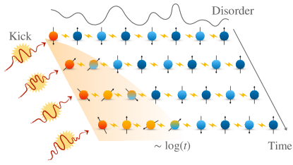
Figure 1: Graphical visualization of the model: a 1D chain of interacting 1/2 spins with a fixed disorder profile, starting from the Néel state, and with open boundary conditions. Different copies of the system mean different subsequent times, as indicated by the time arrow on the right. The leftmost spin is coupled to a $T=\infty$ thermal bath (a time-dependent kick) and a thermalization front (shaded area) propagates logarithmically slowly.

The paper is organized as follows. In Sec. II we define our model, and in Sec. III we discuss the numerical methods we use in the case of many-body localization. In Sec. IV.1 we numerically show that the imbalance thermalization time is exponential both in the system size and in the disorder strength, and this allows us to show that there is a critical strength beyond which MBL is robust against the avalanche instability. In Sec. IV.2 we define a thermalization length scale using the local magnetizations and show that it logarithmically increases with time. This implies that the thermalization time of the imbalance exponentially increases with system size. In Sec. V we consider the mutual information and use it to define another thermalization length scale that also increases logarithmically with time. In Sec. VI we draw our conclusions and sketch perspectives of future work. In the Appendixes we discuss some important aspects that would have broken the main discussion. In particular, in Appendix A we review how the Hamiltonian quantum-trajectory approach works, in Appendix B we discuss how the Gaussian nature of the state in the case of the Anderson model simplifies the numerical analysis, and in Appendix C we review the derivation of the threshold above which the scaling of the slowest thermalization time is slow enough to guarantee robustness against avalanches.

II Model

We consider the 1D spin-1/2 XXZ Heisenberg model in a random magnetic field

$$\hat{H}_{0}=\sum_{j=1}^{L}h_{j}\hat{S}_{j}^{z}+J\sum_{j=1}^{L-1}(\hat{S}^{x}_{j}\hat{S}^{x}_{j+1}+\hat{S}^{y}_{j}\hat{S}^{y}_{j+1}+\Delta\hat{S}^{z}_{j}\hat{S}^{z}_{j+1}),$$ (1)

where $L$ is the system size, $\hat{S}^{\alpha}_{j}\equiv\hat{\sigma}_{j}^{\alpha}/2$ are the on-site magnetizations ($\alpha\in\{x,y,z\}$) and $J=1$ sets the energy scale. The on-site magnetic field $h_{j}$ are chosen randomly and uniformly in the interval $[-W,W]$, and the system conserves the total magnetization $S^{z}_{\rm tot}=\sum_{j=1}^{L}\hat{S}^{z}_{j}$ in the $z$-direction. We consider open boundary conditions.

This model was widely studied as a paradigmatic model displaying MBL behavior [28, 64, 23, 65, 66, 67, 68, 69, 64] for several reasons. It exhibits a transition from the ergodic to the MBL phase at a critical disorder strength $W_{c}$, and it is believed to capture all essential properties of the MBL phase and of the localization transition. At $\Delta=1$ various estimates of $W_{c}$ have been made collocating $3.5\lesssim W_{c}\lesssim 5.4$ [24, 28, 22, 70, 71], although the debate is still open. Furthermore, the Jordan-Wigner transformation [72] allows to map this model to a system of interacting spinless fermions with tunneling matrix element $J$ and nearest-neighbor interaction strength $\Delta$ (see Appendix B for details), connecting the model and the experiments on quasirandom optical lattices [16].

We couple one end of this system to a thermal bath that induces $T=\infty$ thermalization. This evolution is described by the Lindbladian

$$\dot{\hat{\rho}}(t)=-i[\hat{H}_{0},\hat{\rho}(t)]-\gamma^{2}[\hat{S}^{z}_{1},[\hat{S}^{z}_{1},\hat{\rho}(t)]]\,,$$ (2)

where $\gamma^{2}$ is the coupling to the bath. Restricting to any $S^{z}_{\rm tot}$ subspace, one can see that the identity is the only steady state of this Lindblad dynamics, implying the $T=\infty$ thermalization inside that subspace. A similar Lindbladian, acting on all the sites and not just on the first one, has been studied in [62].

In order to study this Lindbladian, we use a quantum trajectory approach. More specifically we rely on the so-called unitary unraveling [63] where the dynamics of Eq. (2) is described by an average over many realizations of unitary Schrödinger evolutions with a noisy Hamiltonian. So one should evolve with the kicked Hamiltonian

$$\hat{H}_{\gamma}(t)=\hat{H}_{0}+\gamma\xi(t)\hat{S}_{1}^{z}\,,$$ (3)

where $\hat{H}_{0}$ is defined in Eq. (1) and $\xi(t)$ is an uncorrelated Gaussian noise, for which $\braket{\xi(t)}=0$, $\braket{\xi(t)\xi(t^{\prime})}=\delta(t-t^{\prime})$ and all the cumulants are vanishing (angular brakets denote the average over noise realizations). In order to implement it numerically, we must discretize it over time intervals $\tau\ll 1/J$ and Trotterize it, so that the $n$-th evolution step is given by the action of the operator

$$\hat{U}_{n}=e^{-i\eta_{n}\gamma\hat{S}_{1}^{z}}e^{-i\tau\hat{H}_{0}}\,,$$ (4)

where $\eta_{n}$ are Gaussian random variables such that $\eta_{n}=\int_{(n-1)\tau}^{n\tau}\xi(t)dt$, so that $\braket{\eta_{n}}=0$ and $\braket{\eta_{n}\eta_{n^{\prime}}}=\tau\delta_{n,n^{\prime}}$. In the following we fix $\tau=0.05$ (choosing a shorter $\tau$ does not affect the results). Averaging over random realizations, in the limit $\tau\to 0$ one recovers the Lindblad equation, Eq. (2), as we show in Appendix A, and in the Anderson-model case $\Delta=0$ the dynamics along each trajectory is given by Gaussian states, allowing thereby to numerically address large system sizes , as we discuss in detail in Appendix B.

III Methods

For the dynamics, it is customary to evolve the system starting from the antiferromagnetic Néel state $\ket{\psi}=\ket{\uparrow\downarrow\dots\uparrow\downarrow}$, which has total magnetization $S_{\rm tot}^{z}=0$ and is included in the smaller sector of the Hilbert space of dimension $\mathcal{N}=\binom{L}{L/2}$. In order to detect the effect of the kick on the localized chain, we compare two different evolutions, one with the Hamiltonian, Eq. (1), without noise ($\gamma=0$)

$$\ket{\psi_{0}(t)}=e^{-i\hat{H}_{0}t}\ket{\uparrow\downarrow\uparrow\downarrow...}\,,$$ (5)

and one with the fully noisy Hamiltonian $\hat{H}_{\gamma}$ [Eq. (3)], fixing the same disorder realization

$$\ket{\psi_{\gamma}(t)}=\prod_{n=1}^{[t/\tau]}\hat{U}_{n}\ket{\uparrow\downarrow\uparrow\downarrow...}\,,$$ (6)

ending both evolutions at some final time $t_{f}$. The state $\ket{\psi_{0}(t)}$ is unaffected by noise and will be considered as a reference. We average each of the quantities over $N_{r}$ different disorder/noise realizations. When $\gamma=0$ in each realization we take a different random choice of the onsite fields $h_{j}$, for $j\in\{1,\,\ldots,\,L\}$ in Eq. (1). When $\gamma=1$ we take in each realization a different choice of the $h_{j}$ and also a different choice of the random sequence $\eta_{n}$, with $n\in\{1,\ldots,[t_{f}/\tau]\}$ providing the noise in Eq. (4). We indicate the average over the $N_{r}$ disorder/noise realizations with an overline $\overline{(\ldots)}$. We evaluate the errorbar on this average as the root mean square deviation divided by $\sqrt{N_{r}}$, performing error propagation where appropriate.

In the case of the Anderson model we take $N_{r}=1200$ while in the case of MBL, in which the simulation times are longer, the number of realizations will be going from $N_{r}=500$ for the smallest system $L=8$, to $N_{r}=100$ for the biggest one $L=16$. When we compare $\gamma=1$ and $\gamma=0$ we average over the same set of disorder realization. To simulate the time evolution we use exact diagonalization and Krylov subspace projection methods [73]. Exact diagonalization is much more efficient in the case of the Anderson model ($\Delta=0$) thanks to the mapping of each trajectory to a free fermion model (see Sec. B). In the following text, whenever we consider an interacting case, we fix $\Delta=1$, and when we consider coupling to the thermal bath we take $\gamma=1$.

IV Imbalance and local magnetizations

IV.1 Imbalance behavior and robustness against avalanche instability

The imbalance $\mathcal{I}$ between the even and odd sites in the spin representation is defined as

$$\mathcal{I}(t)=\frac{1}{L}\sum_{j=1}^{L}(-1)^{j}\langle\psi(t)|\hat{S}_{j}^{z}|\psi(t)\rangle.$$ (7)

It is a global feature of the system which can be computed from local quantities, and can be experimentally measured [16, 74]. The normalization ensures $\mathcal{I}(t=0)=1$. The long-time stationary value of the imbalance effectively serves as an order parameter of the MBL phase, which is why it has been widely used in the literature [75, 64, 71]. For disorder strength $W<W_{c}$, a power-law decay $\mathcal{I}(t)\propto t^{-\beta}$ has been observed [75], while, in localized ones for $W>W_{c}$, one numerically sees convergence to a constant value at long times [44], indicating the existence of a set of conserved quantities preserving local information about its initial state. (See [64] for the challenges related to numerically observing the latter regime.)

The goal of our analysis is to understand how the imbalance applying the kick $\overline{\mathcal{I}}_{\gamma=1}$ differs from the unbiased case, $\overline{\mathcal{I}}_{\gamma=0}$ , scaling the size of the system $L$ and the strength of the disorder $W$. We show some examples of the behavior of the imbalance in Fig. 2 for $L=16$ and two different values of $W$ [$W=2$ in panel (a) and $W=8$ in panel (b)]. We see that the coupling to the bath $\gamma$ causes $\overline{\mathcal{I}}_{\gamma}(t)$ to deviate from $\overline{\mathcal{I}}_{0}(t)$ starting at a time $t\sim 1$, eventually decaying to zero.

In order to perform a size scaling we define a relative imbalance $\mathcal{I}_{r}$ as

$$\mathcal{I}_{r}(t)=\frac{\overline{I}_{0}(t)-\overline{I}_{\gamma}(t)}{\overline{I}_{0}(t)}\,.$$ (8)

This quantity increases from the initial value $\mathcal{I}_{r}(t=0)=0$ [due to $\overline{\mathcal{I}}_{0}(t=0)=\overline{\mathcal{I}}_{\gamma}(t=0)$] to the asymptotic value $\mathcal{I}_{r}(t\to\infty)=1$ [due to $\overline{\mathcal{I}}_{\gamma}(t\to\infty)=0$], as we see in Fig. 2. We can study the time scale over which this happens and we do that computing the minimum time $\widetilde{t}$ it takes for the relative imbalance $\mathcal{I}_{r}$ to grow above a fixed threshold, within the statistical error. Given the computational limitations, we fixed the common threshold to be $r_{\rm th}=0.17$. [76]

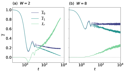
Figure 2: Interacting case. Time evolution of the imbalance in the unkicked case $\overline{\mathcal{I}}_{0}$, in the kicked case $\overline{\mathcal{I}}_{1}$ and relative difference $\mathcal{I}_{r}$ for $L=16$, for $W=2$ in panel (a) and $W=8$ in panel (b), and $N_{r}=100$.

We show results in Fig. 3. From one side we see that $\widetilde{t}$ displays a behavior consistent with an exponential increase with the disorder strength $W$, as the fits in Fig. 3(a) shows. This is in agreement with the exponential dependence on the disorder strength of the thermalization time, seen when one end of a MBL chain is time-periodically coupled to an ergodic one [54]. Furthermore, the exponentially increase with disorder strength is also displayed by the Thouless time $t_{\rm{Th}}$, usually defined as the longest physically relevant relaxation time in the system [77, 78, 79, 80, 44]. From the other side we find that $\widetilde{t}$ also exponentially increases with the size $L$ of the system, as we show in Fig. 3(b).

So we conclude that, at least for the parameters considered in Fig. 3, there is some $\alpha>0$ such that the thermalization time of the imbalance has the behavior

$$\widetilde{t}\sim\exp(\alpha LW)\,.$$ (9)

This numerical finding has interesting implications for the scaling of the slowest thermalization time, a point very important for the robustness of MBL under the effect of avalanches. As shown for instance in Ref. [57], MBL is robust if the slowest thermalization time $t_{s}$ (the one of the spin farthest from the bath) scales faster than $4^{L}$ (see Appendix C for more details). If we have that $\widetilde{t}$ in Eq. (9) scales faster than $4^{L}$, then we expect the same happening for $t_{s}$, since by definition $t_{s}>\widetilde{t}$. This condition leads to

$$W>\widetilde{W}=\frac{2\ln 2}{\alpha}\,.$$ (10)

Indeed, we have numerically verified that for sufficiently large values of $W$, many-body localization (MBL) is robust against avalanche instability. For $W<\widetilde{W}$, MBL might still be stable because the time scale $t_{s}$ might still grow faster than $4^{L}$. In fact, if the scaling behavior observed in Fig. 3 holds over a sufficiently wide range of parameters, there exists a disorder strength beyond which MBL remains robust.

To gain a deeper understanding of the imbalance behavior, we will focus on the properties of the local magnetizations in the next section. This will allow us to observe the propagation of the thermalization front.

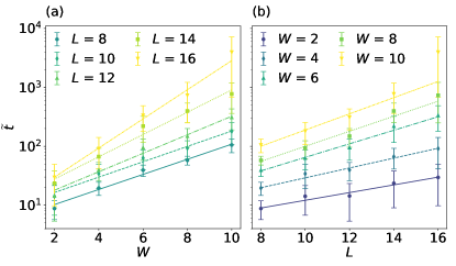
Figure 3: Interacting case. (Panel a) $\widetilde{t}$ versus $W$ for different values of $L$. (Panel b) $\widetilde{t}$ as a function of $L$ for different values of $W$. The error bars are the maximum error, $N_{r}$ goes from $500$ for $L=8$ to $100$ for $L=16$.

IV.2 Thermalization front and local magnetizations

In order to better understand these behaviors of the imbalance, let us consider the local magnetizations $\overline{(S_{j}^{z})}_{\gamma}(t)=\overline{\braket{\psi_{t}}{\hat{S}_{j}^{z}}{\psi_{t}}}$ for the evolution with a given $\gamma$. Let us set

$$\delta S_{j}(t)=\left|\overline{(S_{j}^{z})}_{\gamma=0}(t)-\overline{(S_{j}^{z})}_{\gamma=1}(t)\right|\,,$$ (11)

and use them to see how thermalization propagates through the chain.

In order to do that we define a length scale as

$$h(t)=\frac{\sum_{j=1}^{L}(j-1)\delta S_{j}(t)}{\sum_{j=1}^{L}\delta S_{j}(t)}\,.$$ (12)

We plot $h(t)$ versus $t$ for the Anderson-model case in Fig. 4(a) and in the interacting case in Fig. 4(b). In the Anderson-model case, whatever the disorder strength $W$, we see that $h(t)$ logarithmically increases with time for $t$ large enough, as $h(t)\sim A\ln(t)$, up to a constant, and the same occurs in the interacting case, when $W>W_{c}$ and one is inside the MBL regime. In Fig. 4(b) we also show the behavior for $W=2$ in which $h(t)$ seems to be growing faster than logarithmically and saturating. We can obtain the slope $A$ with a linear fit of $h(t)$ versus $\ln t$. (We apply the fit for times large enough that the linear in $\ln t$ regime has already set in). We plot the $1/A$ resulting from this fit versus $W$ in the insets of Fig. 4. In the Anderson-model case we see that $1/A$ irregularly increases with $W$, while in the interacting case the increase is regular and slightly above a straight line.

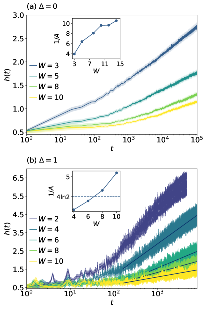
Figure 4: (Main panels) $h(t)$ versus $t$ in the Anderson ($\Delta=0$) case in panel (a) and interacting case ($\Delta=1$) in panel (b). Notice the logarithmic scale on the horizontal axis. (Insets) $1/A$ versus $W$, where $A$ is the slope obtained linearly fitting $h(t)$ versus $\ln t$, applying the fit for times large enough that the linear in $\ln t$ regime has already set in. In the inset in panel (b) the horizontal line marks the reference value $1/A=4\ln 2$, as defined in Eq. (18). Numerical parameters in (a): $L=100,N_{r}=1200$. Numerical parameters in (b): $L=16$, $N_{r}=100$.

So we have a logarithmically propagating thermalization front. This gives rise to some interesting predictions on the behavior of $\mathcal{I}_{r}(t)$. Because at time $t$ only a fraction $f(t)\sim A\ln(t)/L$ of the chain has thermalized, we can predict a behavior

$$\mathcal{I}_{r}(t)\sim A\ln(t)/L\,.$$ (13)

We have obtained this estimate as follows. Due to extensivity, let us write the long-time value of the noiseless imbalance $\overline{I}_{\gamma}(t)=qL$ for some $q\in(0,1)$ and $t\gg 1/J$. If only a fraction of $f(t)$ sites has thermalized, we can roughly approximate $\overline{I}_{\gamma}(t)\sim Lq[1-f(t)]$, and so we apply Eq. (8) and get Eq. (13), valid for $t\gg 1/J$.

We have numerically checked that this prediction is obeyed for large $L$ in the Anderson case as we show in Fig. 5(a), and for smaller system sizes in the interacting case as we show in Fig. 5(b). In both panels we fix $W$ and plot $L\mathcal{I}_{r}(t)$ versus $t$ for different values of $L$, with a logarithmic scale on the horizontal axis. We see that the rescaled curves tend to a limit curve, meaning that the scaling with $1/L$ holds for large system sizes. Furthermore, the limit curve linearly increases with time in logarithmic scale, consistently with Eq. (13). This finding implies an exponential scaling with the system size of the thermalization time of the imbalance, as the one shown in Fig. 3(b).

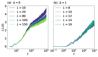
Figure 5: $L\mathcal{I}_{r}(t)$ versus $t$ for and $W=8$ in the Anderson ($\Delta=0$) case in panel (a) and in the interacting case in panel (b). Notice the logarithmic scale on the horizontal axis.

As we can see in the inset of Fig. 4(b), also the behavior of $1/A$ is consistent with a linear increase in $W$. We can therefore write $1/A\sim\beta W$ for some $\beta>0$. Substituting in Eq. (13) and imposing $\mathcal{I}_{r}(\widetilde{t})=r_{\rm th}(=0.17)$ we get

$$\widetilde{t}\sim\exp\left(r_{\rm th}\beta LW\right)\,,$$

that is consistent with Eq. (10).

Let us see what the results above imply for robustness of localization against avalanches. From one side, in the interacting case we have derived Eq. (10), that implies the robustness of MBL for $W$ large enough, as we have see in Sec. IV. From the other let us assume to average over infinite disorder/randomness realization and observe that Eq. (11) implies

$$\delta S_{j}(\infty)=\lim_{t\to\infty}\delta S_{j}(t)=\lim_{t\to\infty}\left|\overline{(S_{j}^{z})}_{\gamma=0}(t)\right|\,,$$ (14)

because $\lim_{t\to\infty}\overline{(S_{j}^{z})}_{\gamma=1}(t)=0$ $\forall j=1,\,\ldots,\,L$ due to thermalization. If we had periodic boundary conditions (PBC), due to the symmetries of the problem averaged over disorder, we would get that the $\left|\overline{(S_{j}^{z})}_{\gamma=0}(t)\right|$ are independent of $j$, and also the $\delta S_{j}(\infty)$ are independent of $j$ (let us write $\delta S_{j}(\infty)\equiv\delta S$). So we get

$$\lim_{t\to\infty}h(t)=\frac{\delta S\sum_{j=1}^{L}(j-1)}{\delta S\sum_{j=1}^{L}1}=\frac{L-1}{2}\quad\text{ for PBC}\,.$$ (15)

Taking open boundary conditions, as we are doing in the numerical analysis above, affects the behavior of the $\left|\overline{(S_{j}^{z})}_{\gamma=0}(t)\right|$, and then of the $\delta S_{j}(\infty)$, for a finite length $l_{b}$ near the boundaries. This length $l_{b}$ is finite and does not scale with $L$ because we are assuming the system with $\gamma=0$ to be localized (Anderson or MBL). So we can write in our case

$$\lim_{t\to\infty}h(t)=\frac{L-1}{2}+\mathcal{O}(l_{b})\,.$$ (16)

In order to find the thermalization time $t^{*}$ we can say that all the local magnetizations have thermalized when $h(t^{*})=\lim_{t\to\infty}h(t)$, and using that, for large enough $t$, $h(t)\sim A\ln(t)$, we get with some simple algebra

$$t^{*}\sim\exp\left(\frac{L}{2A}\right)\,,$$ (17)

with some multiplicative constants in front that are irrelevant for the scaling with $L$. In order to have robustness against avalanches, we must have a scaling faster than $4^{L}$. We meet this condition if $\exp\left(\frac{1}{2A}\right)>4$ or

$$\frac{1}{A}>4\ln 2\,.$$ (18)

In the inset of Fig. 4(a), we observe that the Anderson model consistently satisfies this requirement within the parameter range we investigate. The Anderson model is inherently integrable and unable to generate ergodic inclusions. However, if an ergodic inclusion is introduced into the model, it remains resistant to thermalization induced by avalanches within this parameter range.

In contrast, the MBL model satisfies Eq. (18) provided that $W$ exceeds a threshold value $W^{*}\gtrsim 7$, as shown in the inset of Fig. 4(b). For $W>W^{*}$, MBL remains robust. For $W<W^{*}$, we cannot make definitive claims about stability because $t^{*}$ in Eq. (17) only offers a lower bound on the slowest thermalization time $t_{s}$.

V Quantum mutual information

The quantum mutual information (QMI) for two spatial subsets of the chain $\mathcal{A},\mathcal{B}\subset[1,L]$ is defined as

$$I_{m}(\mathcal{A},\mathcal{B})=S(\mathcal{A})+S(\mathcal{B})-S(\mathcal{A}\cup\mathcal{B}),$$ (19)

where $S(\mathcal{A})$ is the Von Neumann entropy $S(\mathcal{A})=-\text{Tr}(\hat{\rho}_{A}\ln\hat{\rho}_{A})$, $\hat{\rho}_{A(B)}=\operatorname{Tr}_{A(B)}\left[\ket{\psi}\bra{\psi}\right]$ is the reduced density matrix of the subsystem $\mathcal{A}(\mathcal{B})$. The QMI can be used to study the spread of quantum correlations between two separated spatial subsets at distance $j$. More specifically, if $\mathcal{A}\equiv[1]$ is the subsystem only made by the spin in position $1$, and $\mathcal{B}\equiv[1+j]$ is the subsystem only made by the spin at position $1+j$, we define

$$I_{mj}\equiv I_{m}([1],[1+j])\,.$$ (20)

It was shown in Ref. [81] that QMI can be used as a probe to detect MBL.

In the closed system case, $\gamma=0$, $\overline{I_{mj}}(t)$ asymptotically tends to a constant, that depends on the distance $j$ and the strength of the disorder $W$, and is in general smaller than the infinite temperature value. If we apply the kick, the system thermalizes to infinite temperature and the mutual information between any pair of sites becomes a constant independent of the the disorder strength and of the choice of the sites.

In Fig. 6(a) we show an example of $\overline{I_{mj}}(t)$ versus $t$ for $L=14$, $\gamma=1$, $\Delta=1$, $W=1$, for every possible value of $j$, together with the infinite temperature value $T=\infty$. We see that, independently of the distance $j$, at long times all the $\overline{I_{mj}}(t)$ converge to the same limit, that cannot be distinguished on this scale from the $T=\infty$ one. We obtain the $T=\infty$ value with the construction introduced in [82]: We average $I_{mj}$ over random superpositions of spin configurations, each of them being

$$\ket{\psi}=\frac{1}{\sqrt{\mathcal{N}}}\sum_{\{s\}}e^{-i\varphi_{\{s\}}}\ket{\{s\}}$$ (21)

where $\{s\}$ are the spin configurations consistent with vanishing $S^{z}_{\rm tot}$, $\mathcal{N}=\binom{L}{L/2}$ is the dimension of the Hilbert space, and $\varphi_{\{s\}}$ are random numbers uniformly distributed in the interval $[0,2\pi]$. In Fig. 6(b) we see see that the agreement between the asymptotic value and the $T={\infty}$ value improves for increasing system size, in agreement with the fact that fluctuations around the thermal value decrease for increasing system size. We consider here the case $W=1$ because the thermalization time is short, but eventually occurs for generic $W$, due to the thermalization to $T=\infty$ induced by the bath.

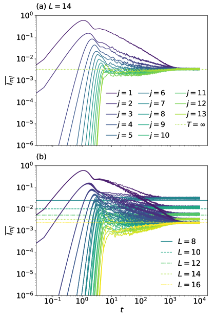
Figure 6: (a) $\overline{I_{mj}}$ as a function of time for $L=14$, $\gamma=1$, $\Delta=1$, $W=1$ ($N_{r}=200$) at every distance $j$ from the site 1, the dotted line is the infinite temperature limit. All the lines at long times converge to the infinite temperature values (straight lines). (b) $\overline{I_{mj}}$, $\gamma=1$, $\Delta=1$, as a function of time at every distance $j$ from the site 1 for systems from size $L=8$ to $L=16$. ($N_{r}$ from 500 to 100). In this case, every fixed distance is plotted for the same color for different system sizes. Infinite temperature values are plotted as straight lines for the different sizes.

In order to track the spreading of the QMI in the system we define the following lengthscale

$$\ell(t)=\frac{\sum_{j=2}^{L}(j-1)\overline{{I_{m}}_{j}}(t)}{\sum_{j=2}^{L}\overline{{I_{m}}_{j}}(t)}\,.$$ (22)

The fact that $\overline{I_{mj}}(t\to\infty)\to\text{const}$ implies that $\lim_{t\to\infty}\ell(t)=L/2$, as this quantity independently of the disorder strength, as one can easily check substituting in Eq. (22) a constant value to $\overline{I_{m}}_{j}(t)$. We plot $\ell(t)$ versus $t$ in Fig. 7(a) for the Anderson model ($\Delta=0$) and in Fig. 7(b) for the interacting model ($\Delta=1$). In the former case we see a logarithmic increase of this quantity in time, whatever the disorder amplitude $W$, while in the latter this logarithmic increase occurs when $W>W_{c}$ and one is inside the MBL regime. We also show an example of behavior for $W<W_{c}$ ($W=2$) in which the growth is faster then logarithmic. In Fig. 7(a) we plot for comparison also a case without thermal bath, where $\ell(t)$ suddenly reaches an asymptotic value much smaller than $L/2$ and does not increase logarithmically in time. In the presence of the thermal bath, we find the slope of the logarithmic increase $\ell(t)\sim B\ln t$ linearly fitting $\ell(t)$ versus $\ln t$. (We apply the fit for times large enough that the linear in $\ln t$ regime has already set in). We find that the inverse slope saturates with in $W$, exactly as the slope of $h(t)$ versus $\ln t$ (see inset of Fig. 4).

Also here, as in Sec. IV.2, we can provide a lower bound to the slowest thermalization time. As we have noticed above, the system asymptotically thermalizes, so in the $t\to\infty$ limit the $\overline{{I_{m}}_{j}}(t\to\infty)$ become uniform, and we see that asymptotically $\ell(t\to\infty)=L/2$. One gets thermalization of the mutual information at the time $t^{*}_{\rm i}$ when this asymptotic behavior is saturated, that is $\ell(t_{\rm i}^{*})=\ell(t\to\infty)$. Because for $t$ large enough we have $\ell(t)=B\ln(t/t_{0,\,{\rm i}})$ for some constant $t_{0,\,{\rm i}}$ (see main panel of Fig. 7), this condition is equivalent to $B\ln(t^{*}_{\rm i}/t_{0,\,{\rm i}})=L/2$, that is to say

$$t^{*}_{\rm i}=t_{0,\,{\rm i}}\exp\left(\frac{L}{2B}\right)\,.$$ (23)

If we impose a scaling faster than $4^{L}$ we find $1/B>4\ln 2$, and – as we can see in the insets of Fig. 7 – this condition is verified for all the parameters we are considering, also in the interacting case [inset of Fig. 7(b)]. So, the analysis of the QMI provides an interval of robustness of MBL larger than the one provided by the analysis of the local magnetizations in Sec. IV.2. We have nevertheless to be cautious with this result, because we are modeling the environment as an average over trajectories. In the case of the local magnetizations it is perfectly equivalent using the Lindbladian or the average over the stochastic Schrödinger equation, because these quantities are linear in the quantum state. By contrast, the QMI is a nonlinear function of the quantum state, and so here we are specifically addressing the properties of the stochastic Schrödinger equation, and that might induce some unknown bias.

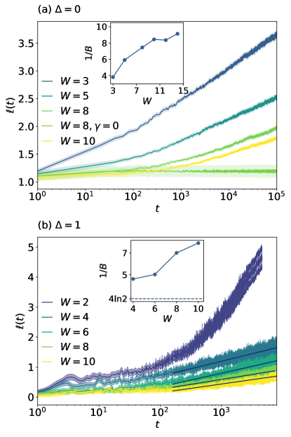
Figure 7: (Main panel) $\ell(t)$ versus $t$ in the Anderson case ($\Delta=0$) in panel (a) and in the interacting case ($\Delta=1$) in panel (b). We display also a case without thermal bath ($\gamma=0$) to show the sudden saturation occurring here. (Inset) For $\gamma=1$ we linearly fit $\ell(t)$ versus $\ln t$ and display the inverse of the slope $1/B$ versus $W$. Numerical parameters in panel (a): $\,L=100,\,N_{r}=1200$. Numerical parameters in panel (b): $\,L=16,\,N_{r}=100$.

VI Conclusion and perspectives

In conclusion we have studied a many-body or Anderson localized model coupled to a $T=\infty$ thermal bath by one end. The coupling is described by a Lindbladian, and to numerically study it we have used a quantum-trajectory approach. More specifically, we have used a unitary unraveling such that the dynamics is an average over many realizations of a unitary Schrödinger evolution with noise. In the case of Anderson localization this approach allows to reach quite large system sizes, due to the Gaussian form of the state along each quantum trajectory.

We have first numerically studied the dynamics of the imbalance, a global quantity widely used to assess the presence of localization. We have defined its thermalization time as the time beyond which the normalized difference of the imbalance with and without thermal bath goes beyond a given threshold, and we see that in the MBL case this thermalization time exponentially increases with the strength of the disorder and the size of the system. We have shown that this result implies that the MBL is robust against the avalanche instability when the disorder strength goes beyond a given threshold.

We have then focused on the heat propagation through the system considering how a thermalization front propagated. We have estimated the extension of the already thermalized part of the chain, defining two length scales using the onsite magnetizations and the quantum mutual information. We have found that they both logarithmically increase with time. This is true both for the MBL case and we could use this fact to lower bound the slowest thermalization time with a quantity exponentially scaling with the system size. We have found that for strong enough disorder strong-disorder regime this scaling is fast enough that the system is robust to avalanches.

The thermalization front propagating logarithmically slowly suggests that the localized integrals of motion might play a role also in case of coupling to a bath, and slow down the heat propagation well below the ballistic trend predicted by the Lieb-Robinson bound [72]. The reason for this idea is that the localized integrals of motion play a strictly similar role in slowing-down the propagation of quantum correlations in an isolated MBL system, that leads to a logarithmic increase of entanglement entropy. Further studies are needed to clarify this point.

Perspectives of future work are exciting. First of all we can focus our attention to the density-density correlator [83], a quantity whose propagation properties are known in MBL systems, and see how its behavior is changed by the presence of a propagating thermalization front. Second we can perform a similar analysis on the OTOC (that for MBL systems has been considered in [84]) to see how the thermalization front affects the scrambling properties of the system. Finally, we can deeper study the relation between strength of localization of the integrals of motion, logarithmic thermalization front, scaling of the slowest thermalization time, and robustness of MBL to avalanches.

Appendix A Derivation of the Lindblad equation form the quantum-trajectory scheme

Let us start with the Schrödinger equation with the Hamiltonian Eq. (3)

$$i\frac{d}{dt}\ket{\psi(t)}=[\hat{H}_{0}+\gamma\xi(t)\hat{S}_{1}^{z}]\ket{\psi(t)}\,.$$ (24)

We can write it as

$$\ket{\psi(t+\Delta t)}\bra{\psi(t+\Delta t)}=\ket{\psi(t)}\bra{\psi(t)}$$ (25)

$$\quad{}-i\Delta t[\hat{H}_{0},\ket{\psi(t)}\bra{\psi(t)}]-i\Delta W_{t}\gamma[\hat{S}_{1}^{z},\ket{\psi(t)}\bra{\psi(t)}]\,,$$

where $\braket{\Delta W_{t}}=\Delta t$ and $\braket{\Delta W_{t}\Delta W_{t^{\prime}}}=\delta_{t,\,t^{\prime}}\Delta t$ are Gaussian uncorrelated variables. Let us also write

$$\ket{\psi(t)}\bra{\psi(t)} =\ket{\psi(t-\Delta t)}\bra{\psi(t-\Delta t)}$$

$$-i\Delta t[\hat{H}_{0},\ket{\psi(t-\Delta t)}\bra{\psi(t-\Delta t)}]$$ (26)

$$-i\Delta W_{t}\gamma[\hat{\sigma}_{1}^{z},\ket{\psi(t-\Delta t)}\bra{\psi(t-\Delta t)}]\,,$$

and substitute it in the last term of Eq. (25). We get many terms. Averaging over randomness and defining $\hat{\rho}_{t}=\big{\langle}\varrho(t)\big{\rangle}$ with $\varrho(t)\equiv\ket{\psi(t)}\bra{\psi(t)}$, we get

$$\hat{\rho}_{t+\Delta t} =\hat{\rho}_{t}-i\Delta t[\hat{H}_{0},\hat{\rho}_{t}]$$

$$\quad{}-(\overline{\Delta W_{t}\Delta W_{t}})\gamma^{2}[\hat{S}_{1}^{z},[\hat{S}_{1}^{z},\hat{\rho}_{t-\Delta t}]]+o(\Delta t)\,.$$ (27)

Using $\braket{\Delta W_{t}\Delta W_{t}}=\Delta t$ and going in the limit $\Delta t\to 0$ we get

$$\frac{d}{dt}\hat{\rho}_{t}=-i[\hat{H}_{0},\hat{\rho}_{t}]-\gamma^{2}[\hat{S}_{1}^{z},[\hat{S}_{1}^{z},\hat{\rho}_{t}]]\,.$$ (28)

Appendix B Case of the Anderson model

Applying the Jordan-Wigner transformation, the model in Eq. (1) becomes the spinless-fermion model

$$\hat{H}_{0}=\sum_{j=1}^{L}h_{j}\hat{n}_{j}+J\sum_{j=1}^{L-1}\left[\frac{1}{2}(\hat{c}_{j}^{\dagger}\hat{c}_{j+1}+{\rm H.\,c.})+\Delta\hat{n}_{j}\hat{n}_{j+1}\right]$$ (29)

where $\hat{c}^{(\dagger)}_{j}$ are anticommuting fermionic operators acting on the $j$-th site. The number of fermions $N\equiv\sum_{j=1}^{L}\hat{n}_{j}$ is conserved. In the Anderson-model case we have $\Delta=0$ and we get a quadratic fermionic Hamiltonian, so that the time evolved state $\ket{\psi(t)}$ along each trajectory can be cast in the form of a generic Gaussian state (Slater determinant). The full information of such state is contained in a $L\times N$ matrix $W(t)$, defined by

$$\ket{\psi(t)}=\prod_{k=1}^{N}\left[\,\sum_{j=1}^{L}\big{[}W(t)\big{]}_{j,k}\,\hat{c}_{j}^{\dagger}\right]\ket{\Omega}\,,$$ (30)

where $\ket{\Omega}$ is the vacuum of the fermionic operators $\hat{c}_{j}$. Because the number of fermions is conserved and we initialize with the Néel state we have $N=L/2$. At initial time, the matrix $L\times N$ matrix defining the Néel state is given by $[W(0)]_{k,l}=\sum_{j=1}^{L/2}\delta_{2j,l}\delta_{j,k}$. The discrete evolution step (see Eq. (4))

$$\ket{\psi({t+\tau})}=e^{-i\eta_{n}\gamma\hat{S}_{1}^{z}}e^{-i\tau\hat{H}_{0}}\ket{\psi(t)}$$ (31)

is simply translated in the dynamics of the matrix $W(t)$ as

$$W(t+\tau)=K_{n}e^{-i\tau Q}W(t)\,,$$ (32)

where the noisy step is implemented through the $L\times L$ diagonal matrix $K_{n}$ with matrix element $[K_{n}]_{i,j}=\delta_{i,j}+\delta_{1,i}\delta_{1,j}(e^{-i\eta_{n}\gamma}-1)$, while the $L\times L$ matrix $Q$ implementing the action of the Anderson Hamiltonian has matrix elements $[Q]_{i,j}=\delta_{i,j}h_{j}+\frac{J}{2}(\delta_{i,j+1}+\delta_{i,j-1})$. Thanks to the validity of Wick’s theorem, one can use the matrix $W(t)$ to obtain the expectation of any observable, and even the entanglement entropy, as clarified in [63]. In this way one can numerically reach quite large system sizes, up to $L\sim\mathcal{O}(10^{2})$.

Appendix C Scaling of the slowest thermalization time and robustness of localization against avalanches

In this section we explain why, in order for localization to be robust against avalanches, the slowest thermalization time should scale faster than $4^{L}$ when one end of the system is coupled to a thermal bath. The thing has already been clearly explained in [57, 55], and we add this section just for completeness. Let us consider Fig. 8 depicting an MBL chain. We have an ergodic inclusion of size $r_{0}$ (red region), and a part that has already thermalize (yellow region) made by two sectors, with the same size $r$ (we assume the avalanches to act symmetrically). The rest of the system is already localized (blue region) and we want to see if thermalization can further propagate there by avalanches.

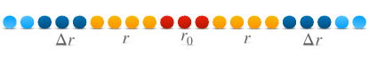
Figure 8: Scheme of an MBL chain for the analysis of robustness of MBL to avalanches. The red region is the ergodic inclusion, the yellow region the thermalized part of the chain, the blue region the part of the chain not yet thermalized. We focus on a subset of the latter (dark blue) that is in contact with the thermalized region and is made by two sectors, each of length $\Delta r$.

With this aim, we focus on a part of the localized region in contact with the ergodic region, made by two sectors of length $\Delta r$ (dark blue region). We ask ourselves if this region thermalizes due to the contact with the yellow region, that’s to say if the avalanche propagates. This can happen if each sector in the dark-blue region (let’s say the right one – they are equal) thermalizes fast enough. So the slowest thermalization time $t_{s}$ of each dark-blue sector must be much shorter than the inverse gap $1/\delta$ of the region obtained joining the red, the yellow and the dark blue regions. The point is that thermalization in each dark-blue sector must be faster than the time needed to the part of the chain involved in the thermalizing dynamics (red+yellow+dark-blue) to express finite-size revivals and other quantum dynamical effects connected with the discreteness of the spectrum that hinder thermalization. On general grounds [57, 55] (and we numerically verify it also in our work) one has $t_{s}\sim\kappa^{\Delta r}$ for some $\kappa>0$. Being this a spin 1/2 system one has $\delta=2^{-(r_{0}+2r+2\Delta r)}$. Imposing $t_{s}\ll 1/\delta$, and asking that this condition should be verified also in the limit of $\Delta r\gg r$, one finds

$$\kappa<4\,.$$ (33)

By contrast, if $\kappa>4$ MBL is robust to avalanches. So it is very important to know $\kappa$. In order to find it, we have done as biologists do when move a portion of neural tissue from in vivo to in vitro [57, 55]: We have cut away the right blue region from the system in Fig. 8, we have connected its left site to a thermal bath simulating the yellow thermalized region in Fig. 8, and we have studied the scaling of the slowest thermalization time with $\Delta r$. (We have renamed $\Delta r$ as $L$ for merely aesthetic reasons.)

References

- Deutsch [1991] J. M. Deutsch, Phys. Rev. A 43, 2046 (1991).
- Srednicki [1994] M. Srednicki, Phys. Rev. E 50, 888 (1994).
- Prosen [1999] T. c. v. Prosen, Phys. Rev. E 60, 3949 (1999).
- Polkovnikov et al. [2011] A. Polkovnikov, K. Sengupta, A. Silva, and M. Vengalattore, Rev. Mod. Phys. 83, 863 (2011).
- Luca D’Alessio and Rigol [2016] A. P. Luca D’Alessio, Yariv Kafri and M. Rigol, Advances in Physics 65, 239 (2016).
- Rigol et al. [2008] M. Rigol, V. Dunjko, and M. Olshanii, Nature 452, 854 (2008).
- Reimann [2016] P. Reimann, Nature Communications 7, 10.1038/ncomms10821 (2016).
- Serbyn et al. [2014] M. Serbyn, M. Knap, S. Gopalakrishnan, Z. Papić, N. Y. Yao, C. R. Laumann, D. A. Abanin, M. D. Lukin, and E. A. Demler, Phys. Rev. Lett. 113, 147204 (2014).
- Anderson [1958] P. W. Anderson, Phys. Rev. 109, 1492 (1958).
- Fleishman and Anderson [1980] L. Fleishman and P. W. Anderson, Phys. Rev. B 21, 2366 (1980).
- Basko et al. [2006] D. Basko, I. Aleiner, and B. Altshuler, Annals of Physics 321, 1126 (2006).
- Gornyi et al. [2005] I. V. Gornyi, A. D. Mirlin, and D. G. Polyakov, Phys. Rev. Lett. 95, 206603 (2005).
- Vosk and Altman [2013] R. Vosk and E. Altman, Phys. Rev. Lett. 110, 067204 (2013).
- Vosk et al. [2015] R. Vosk, D. A. Huse, and E. Altman, Phys. Rev. X 5, 031032 (2015).
- Imbrie [2016] J. Z. Imbrie, Journal of Statistical Physics 163, 998 (2016).
- Schreiber et al. [2015] M. Schreiber, S. S. Hodgman, P. Bordia, H. P. Lüschen, M. H. Fischer, R. Vosk, E. Altman, U. Schneider, and I. Bloch, Science 349, 842 (2015).
- yoon Choi et al. [2016] J. yoon Choi, S. Hild, J. Zeiher, P. Schauß, A. Rubio-Abadal, T. Yefsah, V. Khemani, D. A. Huse, I. Bloch, and C. Gross, Science 352, 1547 (2016), https://www.science.org/doi/pdf/10.1126/science.aaf8834 .
- Smith et al. [2016] J. Smith, A. Lee, P. Richerme, B. Neyenhuis, P. W. Hess, P. Hauke, M. Heyl, D. A. Huse, and C. Monroe, Nature Physics 12, 907 (2016).
- Bordia et al. [2017] P. Bordia, H. Lüschen, U. Schneider, M. Knap, and I. Bloch, Nature Physics 13, 460 (2017).
- Lukin et al. [2019] A. Lukin, M. Rispoli, R. Schittko, M. E. Tai, A. M. Kaufman, S. Choi, V. Khemani, J. Léonard, and M. Greiner, Science 364, 256 (2019).
- Rubio-Abadal et al. [2019] A. Rubio-Abadal, J.-y. Choi, J. Zeiher, S. Hollerith, J. Rui, I. Bloch, and C. Gross, Phys. Rev. X 9, 041014 (2019).
- Oganesyan and Huse [2007] V. Oganesyan and D. A. Huse, Phys. Rev. B 75, 155111 (2007).
- Žnidarič et al. [2008] M. Žnidarič, T. c. v. Prosen, and P. Prelovšek, Phys. Rev. B 77, 064426 (2008).
- Pal and Huse [2010] A. Pal and D. A. Huse, Phys. Rev. B 82, 174411 (2010).
- Bauer and Nayak [2013] B. Bauer and C. Nayak, Journal of Statistical Mechanics: Theory and Experiment 2013, P09005 (2013).
- Luca and Scardicchio [2013] A. D. Luca and A. Scardicchio, Europhysics Letters 101, 37003 (2013).
- Kjäll et al. [2014] J. A. Kjäll, J. H. Bardarson, and F. Pollmann, Phys. Rev. Lett. 113, 107204 (2014).
- Luitz et al. [2015] D. J. Luitz, N. Laflorencie, and F. Alet, Phys. Rev. B 91, 081103 (2015).
- Artiaco et al. [2022] C. Artiaco, F. Balducci, M. Heyl, A. Russomanno, and A. Scardicchio, Phys. Rev. B 105, 184202 (2022).
- Artiaco et al. [2024] C. Artiaco, C. Fleckenstein, D. Aceituno Chávez, T. K. Kvorning, and J. H. Bardarson, PRX Quantum 5, 020352 (2024).
- Bar Lev et al. [2015a] Y. Bar Lev, G. Cohen, and D. R. Reichman, Phys. Rev. Lett. 114, 100601 (2015a).
- Iemini et al. [2016] F. Iemini, A. Russomanno, D. Rossini, A. Scardicchio, and R. Fazio, Phys. Rev. B 94, 214206 (2016).
- Doggen et al. [2021] E. V. Doggen, I. V. Gornyi, A. D. Mirlin, and D. G. Polyakov, Annals of Physics 435, 168437 (2021), special Issue on Localisation 2020.
- Serbyn et al. [2013a] M. Serbyn, Z. Papić, and D. A. Abanin, Phys. Rev. Lett. 111, 127201 (2013a).
- Huse et al. [2014] D. A. Huse, R. Nandkishore, and V. Oganesyan, Phys. Rev. B 90, 174202 (2014).
- Imbrie et al. [2017] J. Z. Imbrie, V. Ros, and A. Scardicchio, Annalen der Physik 529, 1600278 (2017).
- Chiara et al. [2006] G. D. Chiara, S. Montangero, P. Calabrese, and R. Fazio, Journal of Statistical Mechanics: Theory and Experiment 2006, P03001 (2006).
- Eisert et al. [2010] J. Eisert, M. Cramer, and M. B. Plenio, Rev. Mod. Phys. 82, 277 (2010).
- Bardarson et al. [2012] J. H. Bardarson, F. Pollmann, and J. E. Moore, Phys. Rev. Lett. 109, 017202 (2012).
- Serbyn et al. [2013b] M. Serbyn, Z. Papić, and D. A. Abanin, Phys. Rev. Lett. 110, 260601 (2013b).
- Roy et al. [2015] D. Roy, R. Singh, and R. Moessner, Physical Review B 92, 10.1103/physrevb.92.180205 (2015).
- Alet and Laflorencie [2018] F. Alet and N. Laflorencie, Comptes Rendus Physique 19, 498 (2018).
- Abanin et al. [2019] D. A. Abanin, E. Altman, I. Bloch, and M. Serbyn, Rev. Mod. Phys. 91, 021001 (2019).
- Sierant et al. [2024] P. Sierant, M. Lewenstein, A. Scardicchio, L. Vidmar, and J. Zakrzewski, arXiv e-prints 10.48550/arXiv.2403.07111 (2024).
- De Roeck and Huveneers [2017] W. De Roeck and F. m. c. Huveneers, Phys. Rev. B 95, 155129 (2017).
- Gopalakrishnan and Huse [2019] S. Gopalakrishnan and D. A. Huse, Phys. Rev. B 99, 134305 (2019).
- Agarwal et al. [2017] K. Agarwal, E. Altman, E. Demler, S. Gopalakrishnan, D. A. Huse, and M. Knap, Annalen der Physik 529, 1600326 (2017).
- Potirniche et al. [2019] I.-D. Potirniche, S. Banerjee, and E. Altman, Phys. Rev. B 99, 205149 (2019).
- Szołdra et al. [2024] T. Szołdra, P. Sierant, M. Lewenstein, and J. Zakrzewski, Phys. Rev. B 109, 134202 (2024).
- Léonard et al. [2023] J. Léonard, S. Kim, M. Rispoli, A. Lukin, R. Schittko, J. Kwan, E. Demler, D. Sels, and M. Greiner, Nature Physics 19, 481 (2023).
- Lüschen et al. [2017] H. P. Lüschen, P. Bordia, S. S. Hodgman, M. Schreiber, S. Sarkar, A. J. Daley, M. H. Fischer, E. Altman, I. Bloch, and U. Schneider, Phys. Rev. X 7, 011034 (2017).
- Luitz et al. [2017] D. J. Luitz, F. m. c. Huveneers, and W. De Roeck, Phys. Rev. Lett. 119, 150602 (2017).
- Colmenarez et al. [2024] L. Colmenarez, D. J. Luitz, and W. De Roeck, Phys. Rev. B 109, L081117 (2024).
- Peacock and Sels [2023] J. C. Peacock and D. Sels, Phys. Rev. B 108, L020201 (2023).
- Sels [2022] D. Sels, Phys. Rev. B 106, L020202 (2022).
- Tu et al. [2023] Y.-T. Tu, D. Vu, and S. Das Sarma, Phys. Rev. B 107, 014203 (2023).
- Morningstar et al. [2022] A. Morningstar, L. Colmenarez, V. Khemani, D. J. Luitz, and D. A. Huse, Phys. Rev. B 105, 174205 (2022).
- not [a] Unrelated with the problem of the thermal inclusion, many works have studied the effect on MBL of a bath connected to the whole system [85, 86, 87, 88].
- Gopalakrishnan et al. [2015] S. Gopalakrishnan, M. Müller, V. Khemani, M. Knap, E. Demler, and D. A. Huse, Phys. Rev. B 92, 104202 (2015).
- Crowley and Chandran [2022] P. J. D. Crowley and A. Chandran, SciPost Phys. 12, 201 (2022).
- Ha et al. [2023] H. Ha, A. Morningstar, and D. A. Huse, Phys. Rev. Lett. 130, 250405 (2023).
- Levi et al. [2016a] E. Levi, M. Heyl, I. Lesanovsky, and J. P. Garrahan, Phys. Rev. Lett. 116, 237203 (2016a).
- Cao et al. [2019] X. Cao, A. Tilloy, and A. De Luca, SciPost Phys. 7, 24 (2019).
- Sierant and Zakrzewski [2022] P. Sierant and J. Zakrzewski, Phys. Rev. B 105, 224203 (2022).
- Colmenarez et al. [2019] L. Colmenarez, P. A. McClarty, M. Haque, and D. J. Luitz, SciPost Phys. 7, 064 (2019).
- Sierant and Zakrzewski [2019] P. Sierant and J. Zakrzewski, Phys. Rev. B 99, 104205 (2019).
- Chanda et al. [2020] T. Chanda, P. Sierant, and J. Zakrzewski, Phys. Rev. B 101, 035148 (2020).
- Šuntajs et al. [2020a] J. Šuntajs, J. Bonča, T. c. v. Prosen, and L. Vidmar, Phys. Rev. E 102, 062144 (2020a).
- Serbyn et al. [2016] M. Serbyn, A. A. Michailidis, D. A. Abanin, and Z. Papić, Phys. Rev. Lett. 117, 160601 (2016).
- Sierant et al. [2020a] P. Sierant, M. Lewenstein, and J. Zakrzewski, Phys. Rev. Lett. 125, 156601 (2020a).
- Doggen et al. [2018] E. V. H. Doggen, F. Schindler, K. S. Tikhonov, A. D. Mirlin, T. Neupert, D. G. Polyakov, and I. V. Gornyi, Phys. Rev. B 98, 174202 (2018).
- Lieb et al. [1961] E. Lieb, T. Schultz, and D. Mattis, Annals of Physics 16, 407 (1961).
- Sidje [1998] R. Sidje, ACM Trans. Math. Softw. 24, 130 (1998).
- Bordia et al. [2016] P. Bordia, H. P. Lüschen, S. S. Hodgman, M. Schreiber, I. Bloch, and U. Schneider, Phys. Rev. Lett. 116, 140401 (2016).
- Luitz et al. [2016] D. J. Luitz, N. Laflorencie, and F. Alet, Phys. Rev. B 93, 060201 (2016).
- not [b] For the smaller values of , where relaxation times are shorter, we can use larger threshold, and get clearer exponential increases with than the ones shown in Fig. 3(a).
- Edwards and Thouless [1972] J. T. Edwards and D. J. Thouless, Journal of Physics C: Solid State Physics 5, 807 (1972).
- Thouless [1974] D. Thouless, Physics Reports 13, 93 (1974).
- Šuntajs et al. [2020b] J. Šuntajs, J. Bonča, T. c. v. Prosen, and L. Vidmar, Phys. Rev. E 102, 062144 (2020b).
- Sierant et al. [2020b] P. Sierant, D. Delande, and J. Zakrzewski, Phys. Rev. Lett. 124, 186601 (2020b).
- De Tomasi et al. [2017] G. De Tomasi, S. Bera, J. H. Bardarson, and F. Pollmann, Phys. Rev. Lett. 118, 016804 (2017).
- Page [1993] D. N. Page, Phys. Rev. Lett. 71, 1291 (1993).
- Bar Lev et al. [2015b] Y. Bar Lev, G. Cohen, and D. R. Reichman, Phys. Rev. Lett. 114, 100601 (2015b).
- Slagle et al. [2017] K. Slagle, Z. Bi, Y.-Z. You, and C. Xu, Phys. Rev. B 95, 165136 (2017).
- Fischer et al. [2016] M. H. Fischer, M. Maksymenko, and E. Altman, Phys. Rev. Lett. 116, 160401 (2016).
- Levi et al. [2016b] E. Levi, M. Heyl, I. Lesanovsky, and J. P. Garrahan, Phys. Rev. Lett. 116, 237203 (2016b).
- Everest et al. [2017] B. Everest, I. Lesanovsky, J. P. Garrahan, and E. Levi, Phys. Rev. B 95, 024310 (2017).
- Medvedyeva et al. [2016] M. V. Medvedyeva, T. c. v. Prosen, and M. Žnidarič, Phys. Rev. B 93, 094205 (2016).