Engineering photonic band gaps with a waveguide-QED structure containing an atom-polymer array
Abstract
We investigate the generation and engineering of photonic band gaps in waveguide quantum electrodynamics systems containing periodically arranged atom-polymers. We first consider the configuration of a dimer array coupled to a waveguide. The results show that if the intra- and inter-cell phase delays are properly designed, the center and the width of the band gaps, as well as the dispersion relation of the passbands can be modified by adjusting the intra-cell coupling strength. These manipulations provide ways to control the propagating modes in the waveguide, leading to some interesting effects such as slowing or even stopping a single-photon pulse. Finally, we take the case of the tetramer chain as an example to show that, in the case of a larger number of atoms in each unit cell, tunable multi-gap structures and more sophisticated band-gap engineering can be realized. Our proposal provides efficient ways for photonic band-gap engineering in micro- and nano-quantum systems, which may facilitate the manipulation of photon transport in future quantum networks.
I Introduction
Waveguide quantum electrodynamics (wQED) systems are realized by strongly coupling quantum emitters (e.g., atoms, artificial atoms, cavities, and so on) to a one-dimensional (1D) waveguide and are ideal platform for the manipulation of strong emitter-photon interactions Roy et al. (2017); Gu et al. (2017); Sheremet et al. (2023). The high coupling efficiency between emitters and photonic modes makes wQED setups optimal for single-photon level quantum devices Shen and Fan (2005a); Chang et al. (2006); Shen and Fan (2007); Zhou et al. (2008); Astafiev et al. (2010); Shi et al. (2015). In a 1D wQED setup containing multiple emitters, the coherent and dissipative interactions between them can be mediated by their common electromagnetic environment, giving rise to a large number of intriguing phenomena, including superradiant and subradiant phenomena Dicke (1954); Vetter et al. (2016); van Loo et al. (2013); Zhang and Mølmer (2019); Ke et al. (2019); Wang et al. (2020), long-range quantum entanglement between atoms Zheng and Baranger (2013); Gonzalez-Ballestero et al. (2014); Facchi et al. (2016); Mirza and Schotland (2016), cavity QED with atomic mirrors Chang et al. (2012); Mirhosseini et al. (2019); Nie et al. (2023), decoherence-free interactions in giant artificial atoms Kockum et al. (2018), topologically protected scattering spectra Nie et al. (2021), multiple Fano interferences Tsoi and Law (2008); Liao et al. (2015); Cheng et al. (2017); Ruostekoski and Javanainen (2017); Mukhopadhyay and Agarwal (2019), control-field-free atomic coherence effects Mukhopadhyay and Agarwal (2020); Ask et al. ; Jia and Cai (2022); Feng and Jia (2021), and so on.
In recent years, considerable attention has been devoted to photonic band-gap materials in micro- and nano-quantum structures. One potential avenue for achieving this objective is through the use of a conventional photonic crystal waveguide (PCW) Bendickson et al. (1996); Hood et al. (2016), in which the periodicity of the dielectric structure is employed to generate a set of Bloch bands. Moreover, in the microwave domain, PCW has a series of circuit versions, including, for example, coplanar waveguide with periodically modulated impedance Liu and Houck (2017); Sundaresan et al. (2019), resonator array waveguide Kim et al. (2021); Ferreira et al. (2021); Scigliuzzo et al. (2022); Zhang et al. (2023), and circuit-crystal metamaterials with Josephson junction arrays Rakhmanov et al. (2008); Hutter et al. (2011); Zueco et al. (2012). Another method to generate photonic band gaps is based on wQED structures with periodically arranged emitters (either an atom array or a cavity array) side coupled to a 1D linear waveguide Xu et al. (2000); Shen and Fan (2005b); Yanik et al. (2004); Shen et al. (2007); Yi et al. (2010); Witthaut and Sørensen (2010); Fang and Baranger (2015); Mirza et al. (2017); Mirhosseini et al. (2018); He et al. (2021); Greenberg et al. (2021); Tang et al. (2022); Peng and Jia (2023); Berndsen and Mirza (2023); Berndsen et al. (2024). Achieving highly tunable band-gap modulation in periodic structures that have already been prepared is of significant importance. This type of band-gap engineering can facilitate the manipulation of photon transport and the control of light-matter interactions in a variety of ways. In the case of band-gap structures produced by wQED containing multiple atoms, existing schemes for band-gap modulation are mainly based on the adjustment of the atomic frequency Shen et al. (2007); He et al. (2021); Greenberg et al. (2021) and the application of an external control field Witthaut and Sørensen (2010).
In micro- and nano-quantum systems, such as superconducting quantum circuits, the tunability of the coupling strength between artificial atoms is a prominent feature Hime et al. (2006); Niskanen et al. (2007); Baust et al. (2015); Zhu and Jia (2019). It seems reasonable to posit that the tunable coupling between atoms can be harnessed to engineer the band-gap structure formed by wQED systems containing an atomic array. In this paper we present a proposal to achieve this goal, as shown schematically in Fig. 1. In our proposal, a periodic atomic array is coupled to a 1D waveguide, with each unit cell containing at least two atoms with tunable couplings between the nearest neighboring atoms, forming a so called polymer. The transfer matrix of the system is derived using the real-space formalism, and then the corresponding scattering coefficients are expressed analytically in terms of Chebyshev polynomials. Using these results, we further analyze the band-gap structures in the scattering spectra and demonstrate the potential for band-gap engineering through the use of interatomic couplings. Specifically, for the case where each cell is an atom-dimer (i.e., a cell with two coupled atoms), band-gap structures with highly tunable center frequencies and widths can be realized by properly adjusting the intra-cell coupling strength and designing the interatomic phase delays. Moreover, these kinds of modulations can also be used to engineer the propagating modes in the passband. In particular, if a band gap is closed at a specific frequency, the Bloch modes in the vicinity of this frequency will become slow modes with a linear dispersion relation. Furthermore, if the width of a passband is dynamically compressed by modulating the coupling strength, the formation of a flat band can enable the setup to slow down or even stop a single-photon pulse at will. Finally, the results for a dimer array can be generalized to the case of a polymer chain with a greater number of atoms in each unit cell. This enables the realization of a tunable multi-band-gap structure and the implementation of more sophisticated band-gap engineering.
The remainder of this paper is organized as follows. In Sec. II, we present a theoretical model that includes the system Hamiltonian and corresponding single-photon transport equations. Furthermore, using the transfer matrix approach, we derive the expressions of the single-photon scattering coefficients. In Sec. III, we present some general discussions on the band-gap structure produced by a wQED system containing a polymerized atomic chain. In Sec. IV, we analyze tunable band-gap structures and propagation-mode control in a wQED system coupled by an atom-dimer chain. In Sec. V, we further examine band-gap engineering in a wQED system containing an atom-tetramer chain. Finally, further discussions and conclusions are given in Sec. VI.
II Theoretical description of single-photon scattering
II.1 Hamiltonian and single-photon transport equations
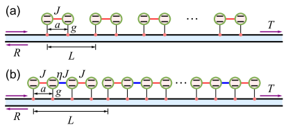
In this study, we concentrate on the wQED structures comprising periodically spaced polymers, each containing two-level atoms with identical transition frequency , coupled to photonic modes in a 1D waveguide with linear dispersion, as schematically shown in Fig. 1. The atoms are located at position ( labels the cells and denotes the atoms in each cell). The lattice constant of the polymer array is . The distance between neighboring atoms in a cell is . The strength between the th atom and the th atom in a cell is . The coupling strength between each atom and the waveguide is . Under the rotating-wave approximation, the Hamiltonian of the system in the real space can be written as :
| (1) |
where and . [] and [] are the bosonic creation (annihilation) operators of the right- and left-going wave at position . is the group velocity of photons in the waveguide. () is the raising (lowering) operator of the th atom in the th cell.
In the single-excitation manifold, the scattering eigenstate can be written as
| (2) |
where is the vacuum state with no photons propagating in the waveguide and the atoms occupying their ground states. is the single-photon wave function in the mode. is the excitation amplitude of the th atom in the th cell.
We assume that a single photon with energy is initially incident from the left, where is the wave vector of the photon. The corresponding right(left)-going wave function [] takes the following Ansatz:
| (3b) | |||||
Here, we define and . () is the transmission (reflection) amplitude of the th atom in the th cell. And the transmission (reflection) amplitude of the last (first) atom () is defined as the transmission (reflection) amplitude of the atom array. denotes the Heaviside step function.
From the eigenequation , we can obtain the following set of equations:
| (4a) | |||
| (4b) | |||
| (4c) | |||
Note that in the above equations the inter-cell connection relations and the boundary conditions are satisfied. is the atomic excitation amplitude scaled by . is the decay rate of the atoms into the guided modes. is the detuning between the photon and the atom. The phase factor corresponding to position is defined as .
II.2 Transfer matrix and scattering coefficients
From Eqs. (4a) and (4b), after iteration, we can obtain
| (5a) | |||
| (5b) |
From now on, we rewrite the phase factor of the th atom in the th cell as . is the reference phase of the th cell (without loss of generality, we have chosen ), where is the phase delay between neighboring cells. is the relative phase of the th atom in each cell with respect to the reference phase, where is the phase delay between neighboring atoms in a unit cell. Note that the phase delays
| (6) |
is detuning dependent, where and are detuning-independent phase delays defined in terms of the frequency of the resonant photons.
Using the above definitions and substituting Eqs. (5a) and (5b) into Eq. (4c), we have
| (7) |
where is the -dimensional identity matrix. is the effective non-Hermitian Hamiltonian of each cell, with elements
| (8) |
and take the form
| (9a) | |||
| (9b) |
According to Eqs (5a) and (5b), we can read the relations satisfied by the transmission (reflection) amplitudes of neighboring cells:
| (10a) | |||
| (10b) |
On the other hand, Eq. (7) allows us to express the vector , which is composed of the excitation amplitudes of the atoms in the th cell, in terms of the corresponding input amplitudes . Substituting this result into Eqs. (10a) and (10b), one can obtain the connection relation between the input and the output amplitudes of the th unit cell
| (11) |
where and the scattering matrix takes the form
| (12) |
Alternatively, the connection relation can be expressed as
| (13) |
Here
| (14) |
represents the transfer matrix, which establishes a relationship between the light field on either side of the th unit cell. As indicated by Eq. (13), the connection relation for a single-polymer setup (i.e., the case of ) with the reference phase set to zero acquires the following form
| (15) |
where and are the corresponding transmission and reflection amplitudes. Furthermore, by inserting Eq. (14) into Eq. (15), it can be observed that
| (16a) | |||
| (16b) |
In addition, the atomic chain under consideration satisfies time reversal symmetry. Consequently, the transfer matrix can also be expressed in terms of and as follows Xu et al. (2000)
| (17) |
Using Eq. (13) iteratively times in succession and noticing the conditions , , , , and , we finally obtain the following connection relation between the reflection and transmission amplitudes for the entire atomic chain:
| (18) |
with
| (19) |
Thus the transmission and reflection amplitudes for the polymer chain read
| (20) |
Notice that the determinant of the matrix is . Based on Abeles’s theorem Abelès, Florin (1950), we can write the matrix in terms of Chebyshev polynomials of the second kind:
| (21) |
with
| (22) |
is the two-dimensional identity matrix. According to Eqs. (20) and (21), one can obtain the transmittance and the reflectance of the polymer chain (see Appendix A for details)
| (23a) | |||
| (23b) |
where . It should be pointed out that the relation is satisfied as a consequence of the conservation of photon number. Therefore, in what follows, we will focus on the reflectance alone when analyzing the band-gap structures.
Moreover, we will focus on the regime where the phase-accumulated effects for detuned photons can be ignored, i.e., one can approximate the detuning-dependent phase delays defined in Eq. (6) as and . Or equivalently, we can say that the Markovian approximation can be performed, i.e., the time delays between the coupling points can be neglected. In Appendix B, we present the Markovian conditions for our system, which are easily satisfied under typical parameters of wQED experiments Sheremet et al. (2023). In what follows, we will use this approximation in our analysis to keep the physics transparent, while in the full numerical calculations we still make the phase delay and depend on the detuning in order to obtain accurate results.
III Formation of band-gap structure
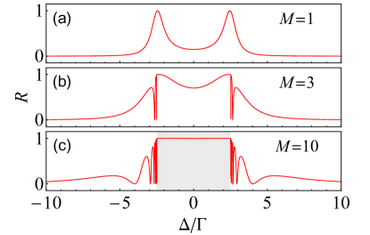
In this section, we present some general discussions on the band-gap structure produced by a polymerized atomic chain. The existence of band gaps is a common feature of periodic structures. For our system, it is not surprising that band-gap structures can form as the number of cells increases. To illustrate this point, we present in Figs. 2(a)-2(c) the reflection spectra for an atom-dimer array for varying values of . As increases, the spectrum with two total reflection points for small evolves into a band-gap structure for relatively large . Moreover, it can be observed from Eq. (23b) that the solutions to the equation for
| (24) |
are the zero points of the function , since () is a root of the the Chebyshev polynomial of the second kind Greenberg et al. (2021); Peng and Jia (2023). Importantly, these zero reflection points outside the band gap indicate the frequencies of the propagating modes that are permitted by the passbands.
In order to gain insight into the formation of the band gap, we consider a periodic chain comprising an adequate number of cells and present the dispersion relation based on Bloch’s theorem (see Appendix C for details):
| (25) |
Here represents the Bloch wave number, which is used to label the propagating modes that are permitted by the wQED system with atomic chain. Clearly, Eq. (25) tells us that for frequencies satisfying the inequality
| (26) |
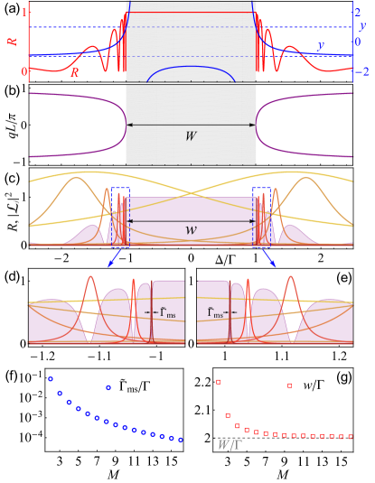
no propagating mode exists, resulting in band-gap structures with in the reflection spectrum, as shown by the shaded region in Fig. 3(a). The corresponding dispersion relation, which can only be defined in the pass bands, is shown in Fig. 3(b).
On the other hand, the formation of a spectrum with band-gap structures can be understood in terms of interference effects between different scattering channels corresponding to the excitations of the collective modes. To this end, we decompose the reflection spectrum into the superpositions of several Lorentzian-type amplitudes contributed by the collective excitations (see Appendix D for details):
| (27) |
Here is the total number of atoms, represents the detuning between the th collective mode and the atoms, denotes the effective decay of the th collective mode, and determines the weight of each Lorentzian component. In Figs. 3(c)-3(e), we illustrate this decomposition by taking the case of a dimer array (with ) as an example. It can can be seen that the Lorentzian-type amplitudes are symmetrically distributed around . The band-gap region with near total reflection is mainly attributed to the excitation of the most superradiant states [see Fig. 3(c)]. While the two narrowest excitation amplitudes corresponding to the most subradiant states are situated at the innermost [see Figs. 3(d) and 3(e)], and the corresponding width, denoted as , decreases sharply with increasing number of cells [see Fig. 3(f)]. The Fano-type destructive interferences between these two most subradiant excitations and the superradiant ones result in the formation of a pair of innermost reflection minima and the corresponding steep band-gap walls [see Figs. 3(c)-3(e)]. This phenomenon becomes more remarkable as the parameter increases. Consequently, as the value of increases to approximately , the distance between the centers of the two innermost amplitudes approaches the width of the band gap [which is obtained from the condition (26)], as shown in Fig. 3(g). This result indicates that the condition (26) can even be used to calculate the gap width of a chain containing a relatively small number of cells.
IV Tunable photonic band gap with a dimer chain
Let us first consider the simplest case of , namely a dimer array coupled to a waveguide, as shown in Fig. 1(a). As demonstrated in the preceding sections, once the expressions for the quantities and [from which we can determine the scattering coefficients (23a) and (23b), as well as the dispersion relation (25)] have been derived, a more comprehensive examination of the scattering spectrum and the band-gap structure is possible. Specifically, in the Markovian regime with and , the quantities and for a dimer array take the form
| (28a) | |||||
| (28b) | |||||
which are strongly influenced by the intra-cell phase difference and the inter-cell phase differences . Here we focus on the cases that the intra- and inter-cell phase delays satisfy either the Bragg or the anti-Bragg condition. The following analysis will demonstrate that, with the exception of the case where both the intra- and inter-cell phase delays satisfy the Bragg condition (see Sec. IV.1), spectra with highly tunable band-gap structures can be generated in the remaining cases by varying the intra-cell coupling strength (see Secs. IV.2-IV.4).
IV.1 and : spectrum with Lorentzian line shape
We begin with the assumption that both the intra- and inter-cell phase differences satisfy the Bragg condition, with () and (, ). Accordingly, Eqs. (28a) and (28b) can be simplified as
| (29a) | |||
| (29b) |
Plugging these expressions into Eq. (23b) and using the identity , the reflectance can be further written as
| (30) |
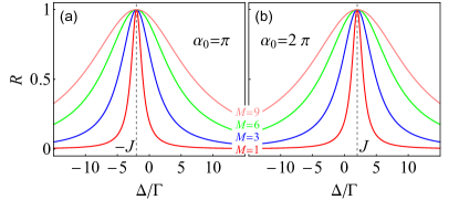
Obviously, similar to an uncoupled atom array (with ) under Bragg condition, the reflection spectrum shows the well-known phenomenon of superradiance, with a line width (scaled as the number of atoms ). However, the center frequency is shifted to instead of at . These properties are shown in Figs. 4(a) and 4(b), where we take the case of () and () as examples.
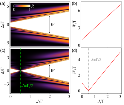
IV.2 and : band gap with tunable width
We proceed to assume that () and (, ), i.e., the intra(inter)-cell phase difference satisfies the anti-Bragg (Bragg) condition. Under these conditions, Eqs. (28a) and (28b) can be simplified as
| (31a) | |||
| (31b) |
After substituting Eq. (31b) into the band-gap condition (26), we find that except for the case of (where the gap is closed), the region of the band gap is
| (32) |
Namely, we can obtain a single band gap centered about , with width
| (33) |
Here “” (“”) corresponds to (). It should be emphasized that the value of do not influence the solution set of the inequality (26), thus the range and width of the band gap are only dependent on the parity of . A similar conclusion can be drawn with regard to the situations discussed in the following subsections (Sec. IV.3 and IV.4). Importantly, the results obtained in Eqs. (32) and (33) indicate that the width of the band gap can be manipulated by changing the coupling strength between the atoms within a cell, which is a significant advantage over a chain of non-interacting atoms.
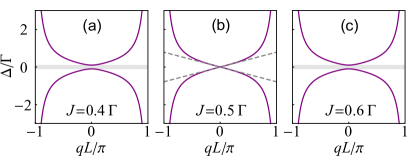
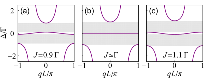
Without loss of generality, we will consider the cases of () and () as illustrative examples to demonstrate the modulation effect of on the width of the band gap. To this end, we plot the reflection spectra and corresponding gap width under these phase delays for varying in Fig. 5. Specifically, when and , the bandwidth increases linearly with . Particularly, if , we can obtain a wide band gap with width [see Figs. 5(a) and 5(b)]. On the other hand, when and , the bandwidth first decreases linearly, reaching a minimum value of zero at , and then increases linearly with to a wide band gap [see Figs. 5(c) and 5(d)]. Additionally, the dispersion relations for this case around are plotted in Figs. 6(a)-6(c). It is shown that at the gap is closed, so the atom-coupled waveguide, like a bare waveguide, allows photons of all frequencies [see Fig. 6(b)]. But its dispersion relation has been greatly modified compared to a bare waveguide. In particular, around the resonance point , one can obtain an effective linear dispersion , with [see the dashed lines in Fig. 6(b)]. Moreover, the ratio between the group velocities of the perturbed and the bare waveguides can be estimated as , which means that under these parameters, the atom-coupled waveguide can be considered as a linear slow-light waveguide.
IV.3 and : band gap with tunable center frequency
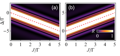
We subsequently discuss the case of () and (, ), i.e., the intra(inter)-cell phase difference satisfies the Bragg (anti-Bragg) condition. Under these conditions, Eqs. (28a) and (28b) can be simplified as
| (34a) | |||
| (34b) |
Similar to Sec. IV.2, with the help of the condition (26), we can find that the region of the band gap is
| (35) |
indicating that the center of the band gap is located at (where “” corresponds to and “” corresponds to ), and the corresponding width is
| (36) |
This result shows that the center of the band gap can be tuned by changing the intra-cell coupling strength . As shown in Figs. 7(a) (with and ) and 7(b) (with and ), due to the existence of the intra-cell coupling, the center of the band gap is red-shifted or blue-shifted by in comparison with a non-interacting atomic chain [see the red dashed lines in Figs. 7(a) and 7(b)], while the width of the band gap remains unchanged.
IV.4 and : tunable double band gaps and center passband
IV.4.1 Tunable band-gap structures
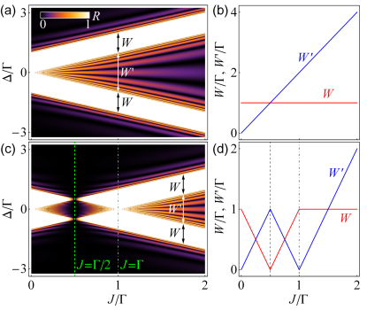
Finally, we discuss the case of () and (, ), i.e., both the intra- and inter-cell phase differences satisfy the anti-Bragg condition. For this case, Eqs. (28a) and (28b) can be simplified as
| (37a) | |||
| (37b) |
For , different from the previous cases, there are always two regions satisfying the condition (26), with
| (38) |
These regions with no propagating modes will form two band gaps centered at with equal width
| (39) |
We refer to them as the right and left band gaps, respectively [see Fig. 8(a)]. And the region between the two gaps forms a passband whose width is proportional to
| (40) |
In a word, we can obtain a symmetrical spectral structure with a passband sandwiched between two band gaps of equal width. In addition, the centers of the gaps, and thus the width of the passband, show a linear relationship with , as shown in Fig. 8(a). To show these more clearly, the widths and as functions of are given in Fig. 8(b).
If , as in the case of , two band-gap regions symmetric about appear in the reflection spectra for different , except for the cases of (where the gaps are closed) and (where the two gaps merge into one). But a richer modulation of the band-gap structure can be obtained by varying the intra-cell coupling strength [see Fig. 8(c)]. According to the condition (26), we can obtain the regions of the gaps, the width of each gap, and the width of the passband between the gaps, as summarized in Table 1. Correspondingly, the widths and as functions of are plotted in Fig. 8(d). Specifically, in the region , the two band gaps are centered at and the width of each gap first decreases linearly (with ) to zero at [where the gaps vanish, see the dashed lines in Figs. 8(c) and 8(d)] and then increases linearly (with ). Finally the two gaps merge into a single band of width at [see the dash-dotted lines in Figs. 8(c) and 8(d)]. Accordingly, the width of the center passband first increases linearly (with ) to a local maximum when (note that at , the center passband cannot be defined because the gaps are closed) and then decreases linearly [with ] to zero at . In the region , the gap splits again into two, centered at and of equal width . And the width of the corresponding center passband increases linearly [with ].
| Range of | Gap regions | |||
IV.4.2 Center passband engineering
Compared to the previous subsections, the most significant feature of the situation now discussed is the possibility of realizing a highly engineered center passband. As we have discussed earlier, its width is easily tunable by the intra-cell coupling strength . Here we will further discuss its other properties. As discussed in Sec. III, the solutions to Eq. (24) can give the zero reflection points in the reflection spectrum. For present case, as shown in Fig. 9, the center branch of can be used to fix the zero reflection points within the passband, which correspond to the propagating modes permitted by this band. According to Eqs. (24) and (25), one can find that the wave numbers of these propagating modes are ().
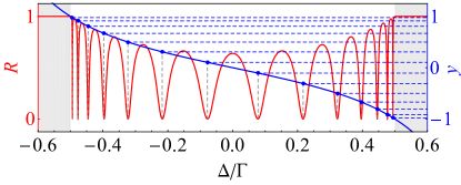
If the frequencies of photons are concentrated within the center passband, the atom-perturbed system can be regarded as a nonlinear waveguide with finite bandwidth, with the group velocity being considerably less than that of the propagating photons in a bare waveguide. By changing , the band width and thus the dispersion relation of the center passband can also be easily engineered. To illustrate, we consider the case of and start with a coupling strength that falls within the range of [see Fig. 10(a)]. Subsequently, the value of is increased until it reaches , during which the bandwidth of the center passband is compressed and ultimately reduces to zero. Consequently, the center passband becomes a flat band, as illustrated in Fig. 10(b). It is evident that, in this situation, the density of the traveling modes becomes exceedingly high, while the group velocity for photons in this band is close to zero. As a result, it is possible to slow or even stop a single-photon pulse at will in this setup by dynamically controlling . If the coupling strength is precisely equal to , the center passband will disappear, as the two gaps will merge into a single gap of width . As the value of is increased to satisfy , the group velocity of the center passband undergoes a change in sign, as illustrated in Fig. 10(c). This indicates that the sign of the group velocity (i.e., the direction of wave-packet propagation) for the passband can also be controlled by selecting an appropriate . We note that similar modulations can also be achieved in a wQED structure containing a resonator array Yanik et al. (2004) or a chain of superconducting qubits Shen et al. (2007) through the appropriate adjustment of the detuning between the emitters in a cell.
Similar to the second case discussed in Sec. IV.2, when and [where the gaps are closed, indicated by the dashed lines in Figs. 8(c) and 8(d)], the atom-coupled waveguide can be utilized as a linear waveguide when the modes in the vicinity of are of interest. When , [the parameters used in Fig. 8(c)], the corresponding dispersion relations in the linear regions can be approximated as and , respectively. Here is the group velocity at of the perturbed waveguide. We also have , which indicates the slow-light effect.
V Tunable photonic band gaps with a polymer chain
The discussions in last section can be generalized to the case of a polymer chain, wherein each unit cell contains a greater number of atoms than two. Naturally, as the number of atoms in a cell increases, multi-band-gap structure can be realized. Furthermore, the design of intra-cell interactions enables the implementation of more sophisticated band-gap engineering. In this section, we utilize the case of a tetramer () array coupled to a waveguide, as shown schematically in Fig. 1(b), as an example to discuss these properties. The coupling strengths between neighboring atoms in a cell are set as and , where the dimensionless parameter is introduced to enhance the tunability of the system. The phase factors are set as and . Correspondingly, the function under the Markovian approximation takes the form
| (41) |
where
Substituting Eq. (41) into the band-gap condition (26), we can obtain the band-gap regions for different values of and . To classify the solutions to the inequality (26), one can define the following discriminant function
| (42) |
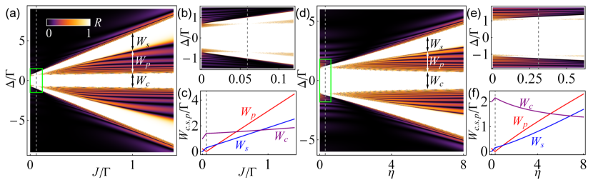
with . For , the reflection spectra indicate that a triple-band-gap structure, comprising a center gap and two side gaps of equal width, is distributed symmetrically about , as shown in Figs. 11(a) (for fixed and varying ) and 11(d) (for fixed and varying ). The details of these spectra around the regions satisfying are provided in Figs. 11(b) and 11(e). Furthermore, both the centers and the widths of the two side gaps and the two passbands between the gaps are highly tunable by varying the values of and . The regions of the gaps, the width of the center gap, the width of the two side gaps, and the width of the two passbands between the gaps are summarized in Table 2. The quantities and in the table take the form
| (43a) | |||
| (43b) |
It can be demonstrated that the relations , , and
are satisfied. In accordance with the reflection spectra illustrated in Figs. 11(a) and 11(d), the widths , , and are plotted as functions of (for fixed ) and of (for fixed ) in Figs. 11(c) and 11(f), respectively. These results show that a tetramer chain can provide greater flexibility in band-gap engineering.
| Condition | Gap regions | ||||
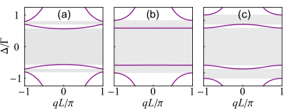
In the case of , the three band gaps merge into a single one centered about , with width , as illustrated by the dashed lines in Figs. 11(a)-11(f). Importantly, if we select an appropriate path in the parameter space spanned by [i.e., from the area satisfying to a point on the curve ], the two passbands between the gaps can be easily compressed and ultimately becomes a flat band when . This property is illustrated in Figs. 12(a)-12(c), in which is held constant while is allowed to vary. Furthermore, the values of and employed in these figures have been selected to satisfy the conditions , , and , respectively. Thus, like the case discussed in Sec. IV.4.2, it is possible to slow or even stop a single-photon pulse by modulating the relevant parameters. However, this time we are able to control the propagation of photon pulses in two distinct passbands simultaneously. Finally, it can be seen from Figs. 12(a) and 12(c) that the group velocities of the two passbands between the gaps can also be designed by selecting suitable values of the parameters and .
VI Conclusions
In this paper, we have analyzed the generation and engineering of photonic band gaps in wQED systems containing multiple atom-polymers. We first consider the configuration of a dimer array coupled to a waveguide with the intra- and inter-cell phase delays satisfying either the Bragg or anti-Bragg condition. It was found that, with the exception of both the intra- and inter-cell phase delays satisfying the Bragg condition, the photonic band-gap structures can be observed in the spectra for the remaining three cases. More importantly, the band-gap structures in these cases can be manipulated in a variety of ways (e.g., the center and the width of the gaps, as well as the dispersion relation of the passbands) by adjusting the intra-cell coupling strength. Furthermore, modulation of the dispersion relation and bandwidth provides an effective way to manipulate the propagating modes in the waveguide, leading to some interesting phenomena such as slowing or even stopping a single-photon pulse. Finally, the results for a dimer array can be generalized to the case of a greater number of atoms in each unit cell. This enables the realization of a tunable multi-gap structure and the implementation of more sophisticated band-gap engineering.
In our proposal, the key point is the use of tunable couplings between atoms to realize band-gap engineering. This can be easily achieved in micro- and nano-quantum systems such as superconducting quantum circuits Gu et al. (2017), where superconducting qubits or superconducting quantum interference devices (SQUIDs) are usually used as tunable coupling elements Hime et al. (2006); Niskanen et al. (2007); Baust et al. (2015); Zhu and Jia (2019). Thus, in summary, we present an experimentally feasible proposal to produce tunable band-gap structures in 1D wQED setups, which may provide novel ways to control single-photon propagation. Our proposal may have potential applications in long-distance quantum networking and quantum communication.
Acknowledgements.
This work was supported by the National Natural Science Foundation of China (NSFC) under Grants No. 61871333.Appendix A Derivation of Eqs. (23a) and (23b)
According to Eq. (21), one can obtain
| (44a) | |||
| (44b) |
Substituting these results into Eq. (20) and taking the square of the modulus yields the transmission and reflection coefficients
| (45a) | |||
| (45b) |
Note that the elements of the transfer matrix satisfy the relation , and [see Eq. (17)]. Thus we have and . Using these results and the identity
| (46) |
the dominator of and can be further simplified as
| (47) | |||||
Finally, by defining the quantity , one can obtain the transmittance and reflectance described by Eqs. (23a) and (23b).
Appendix B The Markovian conditions
In this paper, we focus on the regime in which the detuning-dependent phase delays defined in Eq. (6) can be approximated as and . Here we will present the condition that allows us to make this approximation. The accumulated phase factor between two ends of the atomic chain under consideration in this paper is . Obviously, for a not so small , if the term caused by the detuning effects , it can be safely neglected. Note that for the band-gap cases (the cases in Secs. IV.2-IV.4 and V), the detuning range we are interested in is approximately , and the order of magnitude of we care about is , so we end up with
| (48) |
which is easily satisfied under typical parameters for wQED systems Sheremet et al. (2023). And for the case discussed in Sec. IV.1), we have , the Markovian condition becomes
| (49) |
Furthermore, under these conditions the detuning-dependent term corresponding to any other pair of coupling points can also be ignored, since the distance between them is smaller than the length of the atomic chain. In a word, once the condition (48) (valid for the cases discussed in Secs. IV.2-IV.4 and V) or (49) (valid for the case discussed in Sec. IV.1) is satisfied, we can safely let and .
Appendix C Derivation of dispersion relation
Consider an infinite periotic polymer chain, we write the photonic wave functions to the immediate left and right of the th unit cell as
| (50a) | |||
| (50b) |
According to Bloch’s theorem, we have , where is the Bloch wave number, which leads to the following relations
| (51) |
Substituting Eqs. (17) and (51) into Eq. (13) yields the following linear equations for and :
| (52) |
The non-zero solutions for and requires the determinant of the coefficient matrix to be zero, resulting in the following dispersion relation
| (53) |
Appendix D Expressions of scattering amplitudes in terms of collective modes
By starting from the transport equations (4a)-(4c) and performing some algebra, we can obtain the scattering amplitudes of the atomic chain Peng and Jia (2023)
| (54a) | |||
| (54b) |
Here is the -dimensional identity matrix. is the total number of atoms. takes the form
| (55) |
is the effective non-Hermitian Hamilton matrix of the atomic array, with elements
| (56) |
with . Here the coupling strength between neighboring atoms is defined as and ( and ). The first two terms of Eq. (56) describe the direct atom-atom coupling, and the last term summarizes the atom-waveguide decay (for ) as well as the coherent and dissipative atom-atom interactions mediated by the waveguide modes (for ).
To better understand the physical properties of the scattering process, we rewrite the scattering amplitudes in terms of collective modes of the atomic chain:
| (57a) | |||
| (57b) |
where and are the right and left eigenvectors of the non-Hermitian Hamilton matrix , and and are the corresponding complex eigenvalues, satisfying , , and Brody (2013).
In the Markovian regime we are interested in, the phase accumulation effect caused by the detuned photons can be ignored, thus the quantities , the non-Hermitian Hamiltonian , and the corresponding eigenvalue and eigenvector are independent of the detuning of photons. The transmission and reflection amplitudes [Eqs. (57a) and (57b)] can be further written as
| (58a) | |||
| (58b) |
These results show superpositions of several Lorentzian-type amplitudes contributed by the collective excitations. is the detunning between the th collective mode and the atoms, and is the effective decay of the th collective mode. and determine the weight of each Lorentzian component.
References
- Roy et al. (2017) D. Roy, C. M. Wilson, and O. Firstenberg, Rev. Mod. Phys. 89, 021001 (2017).
- Gu et al. (2017) X. Gu, A. F. Kockum, A. Miranowicz, Y.-x. Liu, and F. Nori, Phys. Rep. 718-719, 1 (2017).
- Sheremet et al. (2023) A. S. Sheremet, M. I. Petrov, I. V. Iorsh, A. V. Poshakinskiy, and A. N. Poddubny, Rev. Mod. Phys. 95, 015002 (2023).
- Shen and Fan (2005a) J.-T. Shen and S. Fan, Phys. Rev. Lett. 95, 213001 (2005a).
- Chang et al. (2006) D. E. Chang, A. S. Sørensen, P. R. Hemmer, and M. D. Lukin, Phys. Rev. Lett. 97, 053002 (2006).
- Shen and Fan (2007) J.-T. Shen and S. Fan, Phys. Rev. Lett. 98, 153003 (2007).
- Zhou et al. (2008) L. Zhou, Z. R. Gong, Y.-x. Liu, C. P. Sun, and F. Nori, Phys. Rev. Lett. 101, 100501 (2008).
- Astafiev et al. (2010) O. Astafiev, A. M. Zagoskin, A. A. Abdumalikov, Y. A. Pashkin, T. Yamamoto, K. Inomata, Y. Nakamura, and J. S. Tsai, Science 327, 840 (2010).
- Shi et al. (2015) T. Shi, D. E. Chang, and J. I. Cirac, Phys. Rev. A 92, 053834 (2015).
- Dicke (1954) R. H. Dicke, Phys. Rev. 93, 99 (1954).
- Vetter et al. (2016) P. A. Vetter, L. Wang, D.-W. Wang, and M. O. Scully, Physica Scripta 91, 023007 (2016).
- van Loo et al. (2013) A. F. van Loo, A. Fedorov, K. Lalumière, B. C. Sanders, A. Blais, and A. Wallraff, Science 342, 1494 (2013).
- Zhang and Mølmer (2019) Y.-X. Zhang and K. Mølmer, Phys. Rev. Lett. 122, 203605 (2019).
- Ke et al. (2019) Y. Ke, A. V. Poshakinskiy, C. Lee, Y. S. Kivshar, and A. N. Poddubny, Phys. Rev. Lett. 123, 253601 (2019).
- Wang et al. (2020) Z. Wang, H. Li, W. Feng, X. Song, C. Song, W. Liu, Q. Guo, X. Zhang, H. Dong, D. Zheng, H. Wang, and D.-W. Wang, Phys. Rev. Lett. 124, 013601 (2020).
- Zheng and Baranger (2013) H. Zheng and H. U. Baranger, Phys. Rev. Lett. 110, 113601 (2013).
- Gonzalez-Ballestero et al. (2014) C. Gonzalez-Ballestero, E. Moreno, and F. J. Garcia-Vidal, Phys. Rev. A 89, 042328 (2014).
- Facchi et al. (2016) P. Facchi, M. S. Kim, S. Pascazio, F. V. Pepe, D. Pomarico, and T. Tufarelli, Phys. Rev. A 94, 043839 (2016).
- Mirza and Schotland (2016) I. M. Mirza and J. C. Schotland, Phys. Rev. A 94, 012302 (2016).
- Chang et al. (2012) D. E. Chang, L. Jiang, A. V. Gorshkov, and H. J. Kimble, New J. Phys. 14, 063003 (2012).
- Mirhosseini et al. (2019) M. Mirhosseini, E. Kim, X. Zhang, A. Sipahigil, P. B. Dieterle, A. J. Keller, A. Asenjo-Garcia, D. E. Chang, and O. Painter, Nature (London) 569, 692 (2019).
- Nie et al. (2023) W. Nie, T. Shi, Y.-x. Liu, and F. Nori, Phys. Rev. Lett. 131, 103602 (2023).
- Kockum et al. (2018) A. F. Kockum, G. Johansson, and F. Nori, Phys. Rev. Lett. 120, 140404 (2018).
- Nie et al. (2021) W. Nie, T. Shi, F. Nori, and Y.-x. Liu, Phys. Rev. Appl. 15, 044041 (2021).
- Tsoi and Law (2008) T. S. Tsoi and C. K. Law, Phys. Rev. A 78, 063832 (2008).
- Liao et al. (2015) Z. Liao, X. Zeng, S.-Y. Zhu, and M. S. Zubairy, Phys. Rev. A 92, 023806 (2015).
- Cheng et al. (2017) M.-T. Cheng, J. Xu, and G. S. Agarwal, Phys. Rev. A 95, 053807 (2017).
- Ruostekoski and Javanainen (2017) J. Ruostekoski and J. Javanainen, Phys. Rev. A 96, 033857 (2017).
- Mukhopadhyay and Agarwal (2019) D. Mukhopadhyay and G. S. Agarwal, Phys. Rev. A 100, 013812 (2019).
- Mukhopadhyay and Agarwal (2020) D. Mukhopadhyay and G. S. Agarwal, Phys. Rev. A 101, 063814 (2020).
- (31) A. Ask, Y.-L. L. Fang, and A. F. Kockum, arXiv:2011.15077 .
- Jia and Cai (2022) W. Z. Jia and Q. Y. Cai, Eur. Phys. J. Plus 137, 1082 (2022).
- Feng and Jia (2021) S. L. Feng and W. Z. Jia, Phys. Rev. A 104, 063712 (2021).
- Bendickson et al. (1996) J. M. Bendickson, J. P. Dowling, and M. Scalora, Phys. Rev. E 53, 4107 (1996).
- Hood et al. (2016) J. D. Hood, A. Goban, A. Asenjo-Garcia, M. Lu, S.-P. Yu, D. E. Chang, and H. J. Kimble, Proc. Natl. Acad. Sci. 113, 10507 (2016).
- Liu and Houck (2017) Y. Liu and A. A. Houck, Nat. Phys. 13, 48 (2017).
- Sundaresan et al. (2019) N. M. Sundaresan, R. Lundgren, G. Zhu, A. V. Gorshkov, and A. A. Houck, Phys. Rev. X 9, 011021 (2019).
- Kim et al. (2021) E. Kim, X. Zhang, V. S. Ferreira, J. Banker, J. K. Iverson, A. Sipahigil, M. Bello, A. González-Tudela, M. Mirhosseini, and O. Painter, Phys. Rev. X 11, 011015 (2021).
- Ferreira et al. (2021) V. S. Ferreira, J. Banker, A. Sipahigil, M. H. Matheny, A. J. Keller, E. Kim, M. Mirhosseini, and O. Painter, Phys. Rev. X 11, 041043 (2021).
- Scigliuzzo et al. (2022) M. Scigliuzzo, G. Calajò, F. Ciccarello, D. Perez Lozano, A. Bengtsson, P. Scarlino, A. Wallraff, D. Chang, P. Delsing, and S. Gasparinetti, Phys. Rev. X 12, 031036 (2022).
- Zhang et al. (2023) X. Zhang, E. Kim, D. K. Mark, S. Choi, and O. Painter, Science 379, 278 (2023).
- Rakhmanov et al. (2008) A. L. Rakhmanov, A. M. Zagoskin, S. Savel’ev, and F. Nori, Phys. Rev. B 77, 144507 (2008).
- Hutter et al. (2011) C. Hutter, E. A. Tholén, K. Stannigel, J. Lidmar, and D. B. Haviland, Phys. Rev. B 83, 014511 (2011).
- Zueco et al. (2012) D. Zueco, J. J. Mazo, E. Solano, and J. J. García-Ripoll, Phys. Rev. B 86, 024503 (2012).
- Xu et al. (2000) Y. Xu, Y. Li, R. K. Lee, and A. Yariv, Phys. Rev. E 62, 7389 (2000).
- Shen and Fan (2005b) J.-T. Shen and S. Fan, Opt. Lett. 30, 2001 (2005b).
- Yanik et al. (2004) M. F. Yanik, W. Suh, Z. Wang, and S. Fan, Phys. Rev. Lett. 93, 233903 (2004).
- Shen et al. (2007) J.-T. Shen, M. L. Povinelli, S. Sandhu, and S. Fan, Phys. Rev. B 75, 035320 (2007).
- Yi et al. (2010) H. Yi, D. S. Citrin, and Z. Zhou, Opt. Express 18, 2967 (2010).
- Witthaut and Sørensen (2010) D. Witthaut and A. S. Sørensen, New J. Phys. 12, 043052 (2010).
- Fang and Baranger (2015) Y.-L. L. Fang and H. U. Baranger, Phys. Rev. A 91, 053845 (2015).
- Mirza et al. (2017) I. M. Mirza, J. G. Hoskins, and J. C. Schotland, Phys. Rev. A 96, 053804 (2017).
- Mirhosseini et al. (2018) M. Mirhosseini, E. Kim, V. S. Ferreira, M. Kalaee, A. Sipahigil, A. J. Keller, and O. Painter, Nat. Commun. 9, 3706 (2018).
- He et al. (2021) S. He, Q. He, and L. F. Wei, Opt. Express 29, 43148 (2021).
- Greenberg et al. (2021) Y. S. Greenberg, A. A. Shtygashev, and A. G. Moiseev, Phys. Rev. A 103, 023508 (2021).
- Tang et al. (2022) J.-S. Tang, W. Nie, L. Tang, M. Chen, X. Su, Y. Lu, F. Nori, and K. Xia, Phys. Rev. Lett. 128, 203602 (2022).
- Peng and Jia (2023) Y. P. Peng and W. Z. Jia, Phys. Rev. A 108, 043709 (2023).
- Berndsen and Mirza (2023) T. Berndsen and I. M. Mirza, Phys. Rev. A 108, 063702 (2023).
- Berndsen et al. (2024) T. Berndsen, N. Amgain, and I. Mirza, J. Opt. Soc. Am. B 41, C9 (2024).
- Hime et al. (2006) T. Hime, P. A. Reichardt, B. L. T. Plourde, T. L. Robertson, C.-E. Wu, A. V. Ustinov, and J. Clarke, Science 314, 1427 (2006).
- Niskanen et al. (2007) A. O. Niskanen, K. Harrabi, F. Yoshihara, Y. Nakamura, S. Lloyd, and J. S. Tsai, Science 316, 723 (2007).
- Baust et al. (2015) A. Baust, E. Hoffmann, M. Haeberlein, M. J. Schwarz, P. Eder, J. Goetz, F. Wulschner, E. Xie, L. Zhong, F. Quijandría, B. Peropadre, D. Zueco, J.-J. García Ripoll, E. Solano, K. Fedorov, E. P. Menzel, F. Deppe, A. Marx, and R. Gross, Phys. Rev. B 91, 014515 (2015).
- Zhu and Jia (2019) Y. T. Zhu and W. Z. Jia, Phys. Rev. A 99, 063815 (2019).
- Abelès, Florin (1950) Abelès, Florin, Ann. Phys. 12, 596 (1950).
- Brody (2013) D. C. Brody, J. Phys. A-Math. Theor. 47, 035305 (2013).