Universal corrections to the superfluid gap in a cold Fermi gas

Abstract

A framework for computing the superfluid gap in an effective field theory (EFT) of fermions interacting via momentum-independent contact forces is developed. The leading universal corrections in the EFT are one-loop in-medium effects at the Fermi surface, and reproduce the well-known Gor’kov-Melik-Barkhudarov result. The complete subleading universal corrections are presented here, and include one-loop effects away from the Fermi surface, two-loop in-medium effects, as well as modifications to the fermion propagator. Together, these effects are found to reduce the gap at low densities. Applications to neutron superfluidity in neutron stars are also discussed.

I Introduction

Dense systems of cold neutrons, as found in, for example, neutron stars and the outer shells of certain heavy-nuclei [1, 2], are believed to be in a superfluid phase. An important quantity that characterizes this phase is the superfluid energy gap $\Delta$, that separates the ground and first excited states in the many-body system. Quantitative knowledge of the gap is needed to understand properties of neutron stars, such as their cooling rates [3] and spin frequency [4]. For recent reviews on the role of superfluidity in neutrons star physics see Refs. [5, 6, 7, 8]. Despite considerable effort by nuclear theorists to compute the superfluid gap in neutron matter, there is little consensus among different techniques [9, 10, 11, 12, 13, 14, 15, 16, 17]. This is likely due to a series of independent complications, including the smallness of the gap energy relative to the scale of the strong interaction, the absence of a clear hierarchy of scales at moderate densities, and the intrinsic complexity of the in-medium interaction. In parallel, there have also been ab initio approaches that determine the gap using Quantum Monte Carlo (QMC) simulations [18, 19, 20, 21]. In principle, these QMC simulations do not rely on uncontrolled approximations, and provide a powerful benchmark for nuclear theorists to compare to.

At very-low temperatures and densities, many-body systems of fermions are universally characterized by a momentum-independent interaction, with a strength proportional to the free-space s-wave scattering length $a$. Relevant to superfluid pairing is the momentum of fermions at the Fermi surface, $k_{F}$, that is related to the number density by $\rho=N/V=k_{F}^{3}/(3\pi^{2})$. In the presence of a Fermi surface, one may then expect to develop a perturbation theory organized in powers of the dimensionless quantity $k_{F}a$, while accounting for the essential singularity at vanishing coupling due to the BCS instability. However, as the BCS instability is inherently non-perturbative [22, 23, 24], the formulation of a perturbative EFT description, which by definition is systematically improvable, is complicated even in the simplest case of a weak finite-range potential [25, 26, 27, 28]. In neutron matter the scattering length is very large, and the densities where such a perturbation theory applies are not of much physical interest. However, in atomic physics, where the scattering length can be tuned with Feshbach resonances [29, 30], the dependence of the gap on $k_{F}a$ is essential to understanding the BCS-BEC crossover [31, 32]. In any case, the simplicity of this universal system offers a useful theoretical laboratory for the development of systematic methods, and will be the focus of this work.

In BCS theory (see App. A for a derivation), the superfluid gap is given in terms of the scattering length by

$$\Delta_{{\rm BCS}}=\frac{8}{e^{2}}\omega_{k_{F}}\exp{\left(\frac{\pi}{2k_{F}a}\right)}\ ,$$ (1)

where $\omega_{k_{F}}\equiv k_{F}^{2}/(2M)$ is the Fermi energy with fermion mass $M$, and $e$ is Euler’s number. The effects of particle-hole screening were computed by Gor’kov-Melik-Barkhudarov (GM) in Ref. [33] leading to the universal suppression,

$$\Delta_{{\rm GM}}\ =\ \frac{1}{(4e)^{1/3}}\Delta_{{\rm BCS}}\ =(0.45138\ldots)\Delta_{{\rm BCS}}\ .$$ (2)

In addition, further subleading corrections have been sketched out and computed for the induced [34] p-wave gaps [35, 36, 37] but, as far as the authors are aware, a full calculation of the subleading contributions to the (s-wave) neutron superfluid gap does not exist.

A goal of this paper is to establish an EFT formulation for calculating the superfluid gap in the case of a momentum-independent potential. In this formulation, the gap is extracted through a singularity analysis of the in-medium four-point correlation function [38], which is determined order-by-order in perturbation theory. Using this formulation, the subleading correction to the s-wave gap is found to be

$$\Delta\ =\ \Delta_{{\rm GM}}\left(1\ +\ \frac{0.95238(40)}{\pi}k_{F}a\ +\ {\mathcal{O}}[(k_{F}a)^{2}]\right)\ .$$ (3)

This result was obtained to very high accuracy by using a technique originally developed in the context of relativistic quantum field theory to numerically evaluate in-medium Feynman diagrams. See App. C for details and references. As $a<0$ (attractive potential), the gap is reduced relative to $\Delta_{\rm GM}$, in agreement with the QMC simulations in Ref. [19].

Although the gap is inherently non-perturbative, the logarithm of the gap has a well-defined expansion in powers of the dimensionless quantity $\lambda=2k_{F}a/\pi$ (this quantity is referred to as the gas parameter in Ref. [39]),

$$\log{\left(\frac{\Delta}{\omega_{k_{F}}}\right)}\ =\ \frac{c_{-1}}{\lambda}\ +\ c_{0}\ +\ c_{1}\lambda\ +\ \ldots$$ (4)

where $c_{n}$ are the coefficients of the terms with $\lambda^{n}$. The result in Eq. (3) gives coefficients of natural size,

$$c_{-1}\ =\ 1\ \ ,\ \ c_{0}\ =\ \frac{7}{3}\left(\log{2}\ -\ 1\right)=-0.71599...\ \ ,\ \ c_{1}\ =\ 0.47619(20)\ .$$ (5)

The basis for the EFT developed in this work is a power counting scheme for collecting the Feynman diagrams that contribute to $\log{\Delta}$ at a given order in $\lambda$. The novel feature utilized here is the explicit tracking of powers of $\lambda$ arising from the BCS singularities in particle-particle loops. By consistently counting powers of $\lambda$, it is clear that the prefactor of the exponential in $\Delta_{{\rm BCS}}$ has no particular meaning as it arises from an inconsistent treatment of perturbation theory: only part of the contributions to $c_{0}$ are taken into account. This has led to confusion in the literature since the GM suppression relative to the BCS prediction is over 50%, and suggests that particle-hole screening is an anomalously large effect. In some sense, the GM result is the true leading order (LO) prediction for the gap, as it is the first order where a quantitative prediction can be made. The coefficient $c_{-1}$ only determines the exponential dependence of the gap, and $c_{0}$ is needed to set the ${\cal O}(1)$ prefactor to the exponential. In this paper, working to LO, NLO and NNLO will correspond to calculating $c_{-1}$, $c_{0}$ and $c_{1}$ respectively.

This paper is organized as follows. Section II reviews the necessary EFT ingredients. The free-space EFT which describes low-energy fermion-fermion scattering is developed in section II.1. This includes the two-body scattering conventions, as well as the scheme used to renormalize the singular interaction. The EFT is then adapted to the in-medium calculation in section II.2. In section III, the perturbative EFT scheme is developed. Section III.1 and III.2 set up the basic methodology that motivates the power-counting scheme presented in section III.3. The NLO calculation is shown to recover the GM result in section III.4, and the NNLO results are summarized in section III.5. Finally, section IV provides a conclusion and a discussion of future related work. Several clarifying derivations, and the bulk of the calculational details are relegated to Appendices.

II EFT Preliminaries

II.1 Free-space EFT

Consider a system of spin-$1/2$ Fermions in vacuum which interact via two-body contact forces. At very low energies, the Lagrange density takes the Galilean invariant form

$${\cal L} = \sum_{\sigma=\uparrow,\downarrow}\Bigg{[}\psi_{\sigma}^{\dagger}\left(i\partial_{t}+\frac{\overrightarrow{\nabla}^{\,2}}{2M}\right)\psi_{\sigma}-\frac{1}{2}g(\psi_{\sigma}^{\dagger}\psi_{\sigma})^{2}\Bigg{]}\,,$$ (6)

where the field $\psi_{\sigma}^{\dagger}$ creates a fermion of spin $\sigma=\uparrow,\downarrow$ and $g$ is the bare coupling constant. The s-wave scattering amplitude corresponding to a momentum independent interaction is

$$T(k)\ =\ -\frac{4\pi}{M}\Big{[}-1/a-ik\Big{]}^{-1},$$ (7)

where $k=\sqrt{ME}$ is the on-shell center-of-mass (c.o.m.) momentum and $a$ is the scattering length. Computing the scattering amplitude in the EFT from the sum of Feynman diagrams shown in Fig. 1 gives

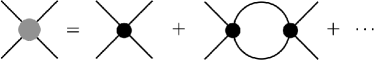
Figure 1: Sum of Feynman diagrams contributing to fermion-fermion scattering. The black blob corresponds to the $g$ interaction from Eq. (6).

$$T(k) = g+g^{2}\,{\mathbb{I}}(k)+g^{3}\,{\mathbb{I}}(k)^{2}+\ldots\ =\ \left(\frac{1}{g}-{\mathbb{I}}(k)\right)^{-1},$$ (8)

where the geometric series has been summed and where the divergent integral

$$\mathbb{I}(k)\equiv\left(\frac{\mu}{2}\right)^{3-d}M\int\!\frac{d^{d}{l}}{(2\pi)^{d}}\,\frac{1}{{k^{2}}-{l^{2}}+i\epsilon}\ \ {\smash{\mathop{{\relbar\joinrel\longrightarrow}}\limits^{\rm PDS}}}\ \ -\frac{M}{4\pi}\left(\mu+ik\right)\ ,$$ (9)

has been evaluated in dimensional regularization with the PDS scheme [40, 41], where $d$ is the number of spatial dimensions and $\mu$ is the renormalization group (RG) scale. Matching the scattering amplitudes in Eqs. (7) and (8) gives

$$\frac{1}{a}=\frac{4\pi}{Mg}+\mu\equiv\frac{4\pi}{Mg_{R}}\ ,$$ (10)

where the renormalized coupling $g_{R}$ has been defined. Note that $\lambda=(M\,k_{F}\,g_{R})/(2\pi^{2})$. For most of the calculations in this work it is convenient to work in the $\overline{\text{MS}}$ scheme where $\mu=0$ and $g_{R}=g$. However, the PDS scheme is useful as a consistency check that the theory is renormalizable; i.e., that all the $\mu$-dependence cancels in physical quantities. In PDS, the bare coupling in the Lagrangian Eq. (6), runs with the RG in such a way to cancel the UV divergences ($\mu$-dependence) coming from the loop integrals. That is,

$$g(\mu)\ =\ \frac{4\pi a}{M}\frac{1}{1-a\mu}\ =\ \frac{4\pi a}{M}\left(1\ +\ a\mu\ -\ {\mathcal{O}}\left[(a\mu)^{2}\right]\right)\ .$$ (11)

In a consistent EFT, observables will be $\mu$-independent at each order in the expansion. This is verified for the gap calculation to NNLO in App. C.

II.2 Finite density EFT

The zero-temperature superfluid gap is traditionally computed in the finite-temperature Matsubara formalism (see App. A) with the zero-temperature limit taken at the end. Here, by contrast, the zero-temperature Feynman diagram expansion will be used to compute the in-medium four-point correlation function. That these two methods lead to equivalent physical results is known as the Kohn-Luttinger-Ward theorem [42, 43], and is discussed at length in the context of the EFT of contact forces in Ref. [27, 44]. A consequence of working in the zero-temperature EFT is that the chemical potential, $\mu_{F}$, is taken to have its own expansion in the interaction strength with the leading contribution given by the Fermi energy (see App. B). The relevant Feynman rules for computing Feynman diagrams in-medium in the EFT at weak coupling can be found in Refs. [45, 27, 38]. In particular, the interaction vertex can be taken from the Lagrange density in Eq. (6), and internal lines are assigned propagators

$$iG_{0}(k_{0},{\bf k})\delta_{\alpha\gamma} =\ i\delta_{\alpha\gamma}\left(\frac{\theta(k-k_{F})}{k_{0}-\omega_{k}+i\epsilon}+\frac{\theta(k_{F}-k)}{k_{0}-\omega_{k}-i\epsilon}\right)$$

$$=\ \delta_{\alpha\gamma}\left(\frac{i}{k_{0}-\omega_{k}+i\delta}-2\pi\delta(k_{0}-\omega_{k})\theta(k_{F}-k)\right)\ ,$$ (12)

where $\alpha$ and $\gamma$ are spin indices, and $\omega_{k}=k^{2}/2M$. The first line splits the propagator between particles and holes and the second line splits the propagator between vacuum and in-medium components [46]. Arrows on fermion lines are used to differentiate particles and holes in in-medium Feynman diagrams.

III Superfluid gap in perturbation theory

III.1 Basic methodology

In a Fermi gas at zero temperature with attractive interactions, superfluid pairing is present between particles with momentum ${\bf k}_{1}$ and ${\bf k}_{2}$ that satisfy ${\bf k}_{1}=-{\bf k}_{2}$ and $k_{1}=k_{2}=k_{F}$. These momenta will be referred to as the “BCS kinematics". Pairing is due to the presence of a Fermi surface, and implies that attractive interactions between particles with BCS kinematics are never “weak". This leads to the formation of Cooper pairs, characterized by strong correlations between pairs of particles in momentum space, and an energy gap $\Delta$ between the ground and first excited state of the Fermi gas.

In many-body perturbation theory, superfluid pairing manifests as a singularity in the 4-point vertex function $\Gamma({\bf k},{\bf k}^{\prime};2E)$, shown to one loop in Fig. 2. At one loop order there is the Zero Sound (ZS) diagram that has particle-hole (p-h) intermediate lines, and the BCS diagram that has particle-particle (p-p) intermediate lines. The strategy for computing $\Delta$ will be to compute $\Gamma({\bf k},{\bf k}^{\prime};2E)$ to a given order in $k_{F}a$, with the gap equal to the imaginary part of the pole in total energy [38, 47, 48] i.e. solves,

$$\left[\Gamma({\bf k},{\bf k}^{\prime};\text{Re}[2E]+i\Delta)\right]^{-1}\ =\ 0\ .$$ (13)

At a practical level, the BCS singularity necessitates the summation of all p-p loops —the so-called ladder diagrams— and therefore pairing is an inherently non-perturbative phenomenon. Despite this proliferation of diagrams, perturbation theory can still be used to determine which diagrams are included at a given order. The power counting used to organize perturbation theory must account for powers of $k_{F}a$ coming both from the bare interaction and from the BCS singularity. The latter contribution is subtle to categorize, and will be motivated with an explicit calculation of $\Gamma$ to LO.

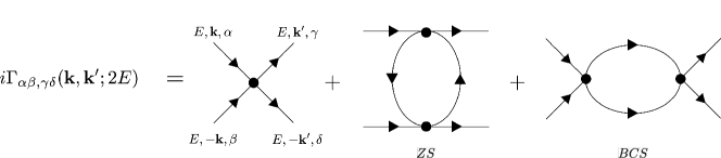
Figure 2: The connected four-point vertex function $\Gamma_{\alpha\beta,\gamma\delta}({\bf k},{\bf k}^{\prime};2E)$ for BCS kinematics to one loop.

III.2 The Gap at LO

For generic kinematics that do not lead to singularities in the BCS or ZS diagrams, the vertex function to LO is simply given by the tree diagram,

$$\Gamma_{\alpha\beta,\gamma\delta}({\bf k},{\bf k}^{\prime};2E)\ =\ -g(\delta_{\alpha\gamma}\delta_{\beta\delta}\ -\ \delta_{\alpha\delta}\delta_{\beta\gamma})\ +\ {\cal O}(g^{2})\ .$$ (14)

For BCS kinematics, it will be shown that p-p loops are no longer suppressed by powers of the coupling due to the BCS singularity. The vertex function to one loop is given by

$$\Gamma_{\alpha\beta,\gamma\delta}({\bf k},{\bf k}^{\prime};2E)\ =\ (-g+g^{2}\Pi_{pp}(E))(\delta_{\alpha\gamma}\delta_{\beta\delta}\ -\ \delta_{\alpha\delta}\delta_{\beta\gamma})$$

$$-\ g^{2}\left(\Pi_{ph}({\bf k},-{\bf k}^{\prime})\delta_{\alpha\gamma}\delta_{\beta\delta}-\Pi_{ph}({\bf k},{\bf k}^{\prime})\delta_{\alpha\delta}\delta_{\beta\gamma}\right)\ ,$$ (15)

where $\Pi_{pp}$ and $\Pi_{ph}$ come from evaluating the loop integrals in the BCS and ZS diagrams respectively; see Fig. 2. The $\Pi_{ph}$ terms do not contain the BCS singularity, and to this order can be dropped. Evaluating the BCS diagram gives

$$\Pi_{pp}(E)\ =\ -i\int\!\frac{d^{4}l}{(2\pi)^{4}}G_{0}(-l_{0},-{\bf l})\,G_{0}(l_{0}+2E,{\bf l})$$

$$=\ -M\int\!\frac{d^{3}{\bf l}}{(2\pi)^{3}}\frac{1}{2ME-l^{2}+i\epsilon}\ +\ 2M\mathchoice{{\vbox{\hbox{$\textstyle-$}}\kern-4.86108pt}}{{\vbox{\hbox{$\scriptstyle-$}}\kern-3.25pt}}{{\vbox{\hbox{$\scriptscriptstyle-$}}\kern-2.29166pt}}{{\vbox{\hbox{$\scriptscriptstyle-$}}\kern-1.875pt}}\!\int\frac{d^{3}{\bf l}}{(2\pi)^{3}}\frac{\theta(k_{F}-l)}{2ME-l^{2}}\ .$$ (16)

The first term in the second line of Eq. (16) is the same as in vacuum, and is given by Eq. (9). The second term in the second line of Eq. (16) has a logarithmic divergence at $2E=2\omega_{k_{F}}$, that is regulated by the imaginary piece of the energy $(i\Delta)$. This singularity can be extracted through an integration by parts [44],

$$2M\mathchoice{{\vbox{\hbox{$\textstyle-$}}\kern-4.86108pt}}{{\vbox{\hbox{$\scriptstyle-$}}\kern-3.25pt}}{{\vbox{\hbox{$\scriptscriptstyle-$}}\kern-2.29166pt}}{{\vbox{\hbox{$\scriptscriptstyle-$}}\kern-1.875pt}}\!\int\frac{d^{3}{\bf l}}{(2\pi)^{3}}\frac{\theta(k_{F}-l)}{2ME-l^{2}}\ =\ \frac{M}{2\pi^{2}}\left[\mathchoice{{\vbox{\hbox{$\textstyle-$}}\kern-4.86108pt}}{{\vbox{\hbox{$\scriptstyle-$}}\kern-3.25pt}}{{\vbox{\hbox{$\scriptscriptstyle-$}}\kern-2.29166pt}}{{\vbox{\hbox{$\scriptscriptstyle-$}}\kern-1.875pt}}\!\int^{k_{F}}_{0}dl\,\log{\left(2ME-l^{2}\right)}\ -\ k_{F}\log{(2ME-k_{F}^{2})}\right]\ .$$ (17)

The first term is finite for $E=\omega_{k_{F}}$, and a perturbatively small $\Delta$ can be expanded in a power series. This is not the case for the second term, which gives $\log\left(iM\Delta\right)$. Looking ahead, the solution for the gap in Eq. (1) reveals that while powers of $\Delta$ are exponentially small in $g$, $\log{\Delta}$ has an expansion in $g$ that starts at ${\cal O}(g^{-1})$. This implies that one can set $E=\omega_{k_{F}}$ everywhere except in terms of the form $\log{(E-\omega_{k_{F}})}$. Combined with the additional factor of $g$ from the vertex, this piece of the p-p loop integral can formally be taken to be of the same order as the tree level contribution. In fact, any number of p-p loops enter at the same order, and LO consists of the sum of an infinite number of diagrams. A key observation, that will simplify higher order calculations, is that the $\log{\Delta}$ piece of this loop integral occurs when the loop momenta are on-shell and at $l=k_{F}$, since it arises from the boundary of the integral.

The p-p loops (ladder diagrams) do not mix partial waves or spin projections, and can be summed as a geometric series,

$$\Gamma_{\alpha\beta,\gamma\delta}({\bf k},{\bf k}^{\prime};2E)\ =\ -\frac{g}{1+g\Pi_{pp}(E)}(\delta_{\alpha\gamma}\delta_{\beta\delta}\ -\ \delta_{\alpha\delta}\delta_{\beta\gamma})\ +\ {\mathcal{O}}(g^{2})\ .$$ (18)

For future convenience, the whole $\Pi_{pp}(E)$ has been resummed, but, to this order, only the $\log{\Delta}$ piece should be kept. Solving Eq. (13) gives

$$0=1-\ g\frac{Mk_{F}}{2\pi^{2}}\log{\Delta}+{\mathcal{O}}(g)\ ,$$ (19)

with solution

$$\Delta_{{\rm LO}}\sim\exp{\left(\frac{\pi}{2k_{F}a}\right)}\ ,$$ (20)

where $g=4\pi a/M$ has been used. Crucially, the prefactor of the exponential cannot be determined at this order. The exponential dependence agrees with Eq. (2), and the resummation of the p-p loops predicated on $\log{\Delta}$ effects beginning at ${\mathcal{O}}(g^{-1})$ is consistent.

III.3 Power Counting

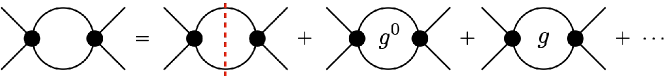
Figure 3: Diagrammatic expansion of the p-p loops in powers of $g$. The red dashed line represents the ${\cal O}(g^{-1})$ contribution that has loop four-momentum at the Fermi surface and on-shell.

The LO calculation presented in the previous section demonstrated that in a consistent power-counting scheme, p-p loops are assigned powers of $g$. To make the power counting manifest, it is beneficial to expand $\Pi_{pp}(E)$ as,

$$\Pi_{pp}(E)\ =\ \Pi^{(g^{-1})}_{pp}\ +\ \Pi^{(g^{0})}_{pp}\ +\ \Pi^{(g)}_{pp}\ +\ldots\ ,$$ (21)

where the $E$ dependence on the RHS has been dropped for simplicity. This is shown diagrammatically in Fig. 3. With this identification, it is possible to collect the Feynman diagrams that contribute to the vertex function $\Gamma$ at a given order in $g$. A key feature is that any sub-diagram connected to $\Pi^{(g^{-1})}_{pp}$ can be evaluated on-shell and at the Fermi surface, since these are the kinematics that give rise to $\log{\Delta}$. This will simplify the NLO and NNLO calculations presented below. The diagrams that contribute to LO and NLO are given in Fig. 5, with sub-diagrams defined in Fig. 4. For the NNLO calculation it is convenient to treat LO, NLO and NNLO together as shown in Fig. 6. A breakdown of the NNLO diagrams is given in Figs. 8 and 9.

III.4 The Gap at NLO

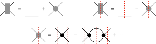
Figure 4: Resummed classes of diagrams. The grey blob is defined in Fig. 1, and a dashed red line corresponds to evaluating the kinematics on-shell and at the Fermi surface. A dashed line running through a p-p loop represents the leading ${\mathcal{O}}(g^{-1})$ contribution.

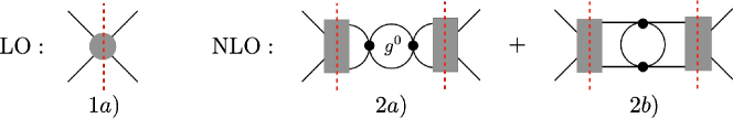
Figure 5: The diagrams that contribute to the vertex function for BCS kinematics at LO and NLO.

At NLO there are two new diagrams contributing to the vertex function, as shown in Fig. 5. Diagram 2a) includes a single insertion of $\Pi^{(g^{0})}_{pp}$, and summing both LO and NLO gives,

$$\Gamma_{1a}+\Gamma_{2a}\ =\ -\frac{g}{1+g\Pi_{pp}^{(g^{-1})}}\left(1-\frac{g\Pi_{pp}^{(g^{0})}}{1+g\Pi_{pp}^{(g^{-1})}}\right)\ .$$ (22)

Diagram 2b) involves an infinite sum of p-p loops, followed by a p-h (ZS) bubble, followed by another infinite sum of p-p loops. At this order, only $\Pi_{pp}^{(g^{-1})}$ contributes to each p-p loop, and therefore the p-h bubble can be evaluated with external legs on-shell and at the Fermi surface. This results in,

$$\Gamma_{2b}\ =\ \frac{-V^{(g^{2})}}{\left(1+g\Pi_{pp}^{(g^{-1})}\right)^{2}}\ ,$$ (23)

where $V^{(g^{n})}$ is the s-wave component of the two-particle irreducible (2PI) potential that scales as $g^{n}$, and is evaluated for external legs on-shell and at the Fermi surface.

The full 2PI potential is determined from the sum of all 2PI diagrams and contains projections onto all partial waves. The ${\mathcal{O}}(g)$ contribution comes from the tree diagram, and the ${\mathcal{O}}(g^{2})$ contribution comes from the ZS diagram in Fig. 2. Evaluating these diagrams in the c.o.m. frame one finds (note the opposite sign relative to $\Gamma$),

$$V^{(g^{2})}_{\alpha\beta,\gamma\delta}({\bf k},{\bf k}^{\prime};\omega)\ =\ g^{2}\left(\Pi_{ph}({\bf k},-{\bf k}^{\prime};\omega)\delta_{\alpha\gamma}\delta_{\beta\delta}-\Pi_{ph}({\bf k},{\bf k}^{\prime};\omega)\delta_{\alpha\delta}\delta_{\beta\gamma}\right)\ ,$$ (24)

where

$$\Pi_{ph}({\bf k},{\bf k}^{\prime};\omega)\ =\ i\int\!\frac{d^{4}l}{(2\pi)^{4}}\left[G_{0}(l_{0},{\bf l})\,G_{0}(l_{0}+\omega,{\bf l}+{\bf k}-{\bf k}^{\prime})\right]$$

$$\stackrel{{\scriptstyle\omega=0}}{{=}}\ -2M\int\!\frac{d^{3}l}{(2\pi)^{3}}\frac{\theta(k_{F}-l)}{({\bf l}-{\bf k})\cdot({\bf k}-{\bf k}^{\prime})}\ ,$$ (25)

with $\omega=k_{0}-k_{0}^{\prime}$ the energy transfer. Relevant for $V^{(g^{2})}$ are kinematics with $k=k^{\prime}=k_{F}$ and $\omega=0$ giving,

$$\Pi_{ph}(q)\ =\ \frac{Mk_{F}}{4\pi^{2}}\left(1\ +\ \frac{4-q^{2}}{4q}\log{\left\lvert\frac{2+q}{2-q}\right\rvert}\right)\ ,$$ (26)

where $q=\lvert{\bf k}-{\bf k}^{\prime}\rvert/k_{F}=\sqrt{2-2\cos{\theta}}$ and $\theta$ is the angle between ${\bf k}$ and ${\bf k}^{\prime}$. The potential can now be expanded onto partial waves as

$$V_{\alpha\beta,\gamma\delta}(\theta)=\begin{cases}\sum_{l}(2l+1)P_{l}(\theta)V_{l}(\delta_{\alpha\gamma}\delta_{\beta\delta}\ -\ \delta_{\alpha\delta}\delta_{\beta\gamma})&l\ {\rm even}\ ,\\[5.0pt] \sum_{l}(2l+1)P_{l}(\theta)V_{l}(\delta_{\alpha\gamma}\delta_{\beta\delta}\ +\ \delta_{\alpha\delta}\delta_{\beta\gamma})&l\ {\rm odd}\ ,\end{cases}$$ (27)

where the $V_{l}$ are obtained by integrating against the relevant Legendre polynomial $P_{l}(\theta)$. Projecting onto the s-wave results in [48, 35]

$$V^{(g^{2})}\ =\frac{g^{2}}{2}\int_{0}^{2}\!dq\,q\Pi_{ph}(q)\ =\frac{Mg^{2}k_{F}}{8\pi^{2}}\frac{4}{3}\left(1\ +\ 2\log{2}\right)\ .$$ (28)

Adding together Eq. (22) and Eq. (23) gives the NLO gap equation,

$$0 =\left[\Gamma_{1a}+\Gamma_{2a}+\Gamma_{2b}\right]^{-1}$$

$$=1+g\left(\Pi_{pp}^{(g^{-1})}+\Pi_{pp}^{(g^{0})}\right)-\frac{V^{(g^{2})}}{g}\ +\ {\mathcal{O}}(g^{2})$$

$$=1+\lambda\left[\log{\left(\frac{8\omega_{k_{F}}}{e^{2}\Delta}\right)}-\frac{1}{3}(1+2\log{2})\right]\ ,$$ (29)

where the quantity

$$g\left(\Pi_{pp}^{(g^{-1})}+\Pi_{pp}^{(g^{0})}\right)\ =\ \lambda\log{\left(\frac{8\omega_{k_{F}}}{e^{2}\Delta}\right)}\ ,$$ (30)

has been determined from the integral in Eq. (16) using the $\overline{\text{MS}}$ scheme. Solving for the gap recovers the GM result [33],

$$\Delta_{\text{NLO}}\ =\ \Delta_{\text{GM}}\ =\ \frac{8\omega_{k_{F}}}{e^{2}(4e)^{1/3}}\exp{\left(\frac{\pi}{2k_{F}a}\right)}\ .$$ (31)

III.5 The Gap at NNLO

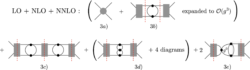
Figure 6: The diagrams that contribute to the vertex function for BCS kinematics through NNLO. The “+ 4 diagrams" corresponds to the 4 other diagrams contributing to the NNLO two-particle-irreducible potential shown in Fig. 9. At this order there are also corrections to the propagator, which affect 3a), and are not explicitly shown.

For the NNLO calculation it is convenient to treat LO, NLO and NNLO together. There are five types of diagrams that contribute to the vertex function, as shown in Fig. 6. The evaluation of the diagrams $\Gamma_{3a,b,c,d,e}$, is treated in App. C, and the NNLO gap equation is

$$0\ =\ \left(\Gamma_{3a}+\Gamma_{3b}+\Gamma_{3c}+\Gamma_{3d}+\Gamma_{3e}\right)^{-1}$$

$$=\ 1+g\left(\Pi_{pp}^{(g^{-1})}+\Pi_{pp}^{(g^{0})}+\Pi_{pp}^{(g)}\right)-\frac{1}{g}\left(V^{(g^{2})}+V^{(g^{3})}\right)+2{\cal I}\left[\Pi^{(g^{0})}_{pp}\,V^{(g^{2})}\right]$$

$$=\ 1+\lambda\left[\log{\left(\frac{8\omega_{k_{F}}}{e^{2}\Delta}\right)}-\frac{1}{3}(1+2\log{2})\right]\ -\ 2.231993(16)\,\lambda^{2}\ +\ 1.83549(20)\,\lambda^{2}\ ,$$ (32)

where ${\cal I}\left[\Pi^{(g^{0})}_{pp}\,V^{(g^{2})}\right]$ accounts for the effects of $V^{(g^{2})}$ evaluated for kinematics away from the Fermi surface. The uncertainties are due to Monte Carlo integration.

At this order, it is also necessary to consider modifications to the propagator, i.e. the self energy. These effects can be parameterized by an effective mass $M^{\star}$ and wavefunction renormalization $Z$ given by [38]

$$\frac{M^{\star}}{M}\ =\ 1+\lambda^{2}\frac{2}{15}(7\log{2}-1)\ +\ \mathcal{O}(\lambda^{3})\ \ ,\ \ Z\ =\ 1-\lambda^{2}\log{2}\ +\ \mathcal{O}(\lambda^{3})\ .$$ (33)

Taking this into account, and solving for the gap, gives

$$\Delta_{\text{NNLO}}\ =\ \frac{8\omega_{k_{F}}}{e^{2}(4e)^{1/3}}(1-0.39650(20)\lambda)\exp{\left(\frac{\pi}{2k_{F}a}\frac{M}{M^{\star}}\frac{1}{Z^{2}}\right)}$$

$$=\frac{8\omega_{k_{F}}}{e^{2}(4e)^{1/3}}(1+0.47619(20)\lambda)\exp{\left(\frac{\pi}{2k_{F}a}\right)}$$

$$=\Delta_{\text{NLO}}\left(1+\frac{0.95238(40)}{\pi}k_{F}a\right)\ .$$ (34)

For an attractive interaction ($a<0$) the gap at NNLO is reduced relative to NLO. In neutron-neutron scattering, the scattering length is $a^{-1}\approx-10.7\,\text{MeV}$ [49], and perturbation theory is expected to break down around $k_{F}\approx 17\,\text{MeV}$.

This result can be compared to Ref. [19] where the gap is determined with QMC. The QMC results have one point at $k_{F}a=-1$ that is expected to be within the perturbative regime. The QMC, NLO and NNLO gaps are:

$$\frac{\Delta_{\text{QMC}}}{\omega_{k_{F}}}\ =\ 0.077(20)\ \ ,\ \ \frac{\Delta_{\text{NLO}}}{\omega_{k_{F}}}\ =\ 0.101592\ \ ,\ \ \frac{\Delta_{\text{NNLO}}}{\omega_{k_{F}}}\ =\ 0.070795(13)\ .$$ (35)

The NLO prediction has slight tension with the QMC result, that goes away at NNLO. More precise QMC simulations across a range of $k_{F}a$ will be needed to confirm the validity of the perturbation theory presented here.

IV Conclusion

The superfluid (or superconducting) gap energy is a hallmark feature of fermions with attractive interactions at finite densities and low temperatures. This work has established an EFT framework for computing the superfluid energy gap for fermions with momentum independent interactions. The momentum independent interaction captures the universal low-energy behavior of fermions with finite range forces, and has applications across a wide range of scales, e.g. to many-body systems of electrons, atoms and/or nucleons. A NNLO calculation in the EFT revealed new, universal corrections, to the GM [33] gap prediction. These corrections decrease the gap, and are found to restore agreement with QMC determinations in Ref. [19]. Using the numerical integration techniques outlined in this paper, and making use of existing higher-order calculations of the self energy [50], it may prove feasible and worthwhile to compute the N³LO corrections to the gap. In addition, this work motivates more precise QMC simulations across a range of $k_{F}a$ to further validate the universal corrections presented here.

In nuclear physics, the s-wave scattering lengths are very large, and the results obtained here are only relevant at very low densities. To access phenomenologically interesting densities found in neutron stars will require a more complex interaction that includes effective range and other momentum-dependent modifications. This can be achieved by treating range corrections in perturbation theory, or by working in an EFT which sums range corrections to all orders [51]. This latter method can be implemented, for instance, by using energy-dependent potentials as in the dimeron method [52], or by using energy-independent separable potentials [53, 54]. Working with such momentum-dependent potentials will likely extend the densities that are accessible to perturbation theory, and will be considered elsewhere.

Appendix A Superfluid gap from the BCS equations

In the presence of a Fermi surface, any attractive interaction leads to superfluidity at zero temperature [24, 23]. The superfluid gap may be obtained from the BCS equations, which are readily derived in the grand canonical ensemble using the Matsubara formalism. Supplementing the Lagrange density, Eq. (6), describing the fermion interactions in free space, with a chemical potential term, $\mu_{F}\psi^{\dagger}\psi$ and transforming to Euclidean space allows the thermodynamic potential $\Omega(\mu_{F},T)$ to be identified with the effective action. A Hubbard-Stratonovich transformation can then be carried out to render the four-fermion interaction quadratic by introducing bosonic fields. Ignoring the fluctuations in the bosonic fields, and evaluating them at their equilibrium values, leads to the BCS mean-field approximation. In particular, minimizing the thermodynamic potential, and taking the zero-temperature limit, one finds the equation for the gap,

$$\Delta({\bf k}) = -\int\!\frac{d^{3}{\bf q}}{(2\pi)^{3}}\,\frac{V\left({\bf k},{\bf q}\right)\Delta({\bf q})}{2\sqrt{\left(\omega_{q}-\mu_{F}\right)^{2}+|\Delta({\bf q})|^{2}}}\ .$$ (36)

For the momentum-independent interaction considered in this work $V\left({\bf k},{\bf q}\right)=g$ . Diagrammatically, this integral equation is given in Fig. 7.

Figure 7: The BCS integral equation for the superfluid gap, represented by the empty triangle.

The equation for the density is finite and obtained by differentiating the thermodynamic potential with respect to $\mu_{F}$:

$$\rho = \frac{k_{F}^{3}}{3\pi^{2}}\ =\ \int\!\frac{d^{3}{\bf q}}{(2\pi)^{3}}\Bigg{[}1\ -\ \frac{\left(\omega_{q}-\mu_{F}\right)}{\sqrt{\left(\omega_{q}-\mu_{F}\right)^{2}+|\Delta({\bf q})|^{2}}}\Bigg{]}\ .$$ (37)

Note that the density of the free Fermi gas is not changed by the interaction, as an interaction that conserves particle number will simply shift the single-particle levels, which in the ground state are still filled up to $k_{F}$.

Choosing the ansatz $\Delta({\bf q})=\hat{\Delta}_{0}(k_{F})$, in the EFT considered here, the gap equation is:

$$\frac{1}{g} = -\left(\frac{\mu}{2}\right)^{3-d}\int\!\frac{d^{d}{\bf q}}{(2\pi)^{d}}\,\frac{1}{2\sqrt{\left(\omega_{q}-\mu_{F}\right)^{2}+\hat{\Delta}_{0}^{2}}}\ .$$ (38)

It is straightforward to evaluate this linearly-divergent integral in DR with PDS [27, 55, 25]. One finds

$$\frac{1}{g_{R}}\;=\;\frac{1}{g}+\frac{M\mu}{4\pi} = \frac{M}{4\pi a}\;=\;\frac{M^{3/2}}{2\sqrt{2}\pi}\mu_{F}^{1/2}\left(1+x^{2}\right)^{1/4}P_{1/2}\left(-\left(1+x^{2}\right)^{-1/2}\right)$$ (39)

where $x\equiv\hat{\Delta}_{0}/\mu_{F}$, $P_{n}$ is a Legendre polynomial, and the renormalization prescription of Eq. (10) has been adopted. Finally, one obtains

$$\frac{1}{(2M\mu_{F})^{1/2}\,a}\;=\;\left(1+x^{2}\right)^{1/4}P_{1/2}\left(-\left(1+x^{2}\right)^{-1/2}\right)\ .$$ (40)

As the right-hand side is negative definite in the interval $0\leq x\leq 1$, this equation has a solution only for $a<0$; that is, for attractive interaction. The equation for the density is finite and is easily solved to give

$$\rho = \frac{k_{F}^{3}}{3\pi^{2}}\ =\ -\frac{(2M\mu_{F})^{3/2}}{4\pi}\left(1+x^{2}\right)^{1/4}\bigg{[}P_{1/2}\left(-\left(1+x^{2}\right)^{-1/2}\right)$$ (41)

$$\qquad\qquad\qquad\qquad\qquad\qquad\ +\ \left(1+x^{2}\right)^{1/2}P_{3/2}\left(-\left(1+x^{2}\right)^{-1/2}\right)\bigg{]}\ .$$

Now, given the fixed inputs $a$ and $M$, and the variable $k_{F}$, the coupled equations, Eq. (40) and Eq. (41), determine $\hat{\Delta}_{0}(k_{F})$ and $\mu_{F}(k_{F})$. As seen above, these results are corrected by in-medium effects which enter as perturbations of the potential (see Fig. 2). Therefore, they rely on the potential being weak, that is, $|k_{F}a|\ll 1$, which is achieved with a small scattering length and/or a small density.

As the gap is expected to vanish for small coupling, the expressions for the gap and for the density should admit an expansion in $x$:

$$\frac{1}{(2M\mu_{F})^{1/2}\,a} = \frac{2}{\pi}\left(2+\log(x/8)\right)\ +\ {\mathcal{O}}(x^{2})\ ,$$ (42)

$$\rho = \frac{k_{F}^{3}}{3\pi^{2}}\ =\ \frac{(2M\mu_{F})^{3/2}}{3\pi^{2}}\ +\ {\mathcal{O}}(x^{2})\ .$$ (43)

Therefore, neglecting ${\mathcal{O}}(x^{2})$ corrections, one finds from the second equation, $\mu_{F}=\omega_{k_{F}}$, and from the first equation, the superfluid gap,

$$\hat{\Delta}_{0}(k_{F})\ =\ \Delta_{{\rm BCS}}\ =\ \frac{8}{e^{2}}\omega_{k_{F}}\exp\left(\frac{\pi}{2k_{F}a}\right)\ .$$ (44)

As the gap is exponentially small when $|k_{F}a|\ll 1$, these results are accurate up to exponentially suppressed effects at weak coupling.

Appendix B Including a chemical potential in the propagator

The energy of particles ${\varepsilon}(k)$ at the Fermi surface is given by the chemical potential ${\varepsilon}(k_{F})=\mu_{F}$. In an interacting system this gets shifted away from $\omega_{k_{F}}$ [38, 44]

$$\mu_{F}\ =\ \omega_{k_{F}}\left(1+\frac{4}{3\pi}k_{F}a\ +\ \frac{4(11-2\log{2})}{15\pi^{2}}(k_{F}a)^{2}+\mathcal{O}[(k_{F}a)^{3}]\right)\ ,$$ (45)

and leads to an overall shift in the denominator relative to the free propagator

$$G(k_{0},{\bf k}) =\ \frac{\theta(k-k_{F})}{k_{0}-\omega_{k}+(\omega_{k_{F}}-\mu_{F})+i\epsilon}+\frac{\theta(k_{F}-k)}{k_{0}-\omega_{k}+(\omega_{k_{F}}-\mu_{F})-i\epsilon}\ .$$ (46)

For the NNLO calculation of the gap, the $k_{F}a$ dependence of $\mu_{F}$ should be kept in the LO and NLO diagrams in Fig. 5 i.e. in $\Pi_{pp}(E)$ and $V^{(g^{2})}$. From Eq. (25) it can be seen that $\mu_{F}$ can be absorbed in a shift of the loop energy variable, and therefore has no effect on $V^{(g^{2})}$.

The $\mu_{F}$ dependence on the gap coming from $\Pi_{pp}(E)$ can be computed explicitly,

$$\Pi_{pp}(E)\ =\ \frac{iM}{4\pi}\sqrt{2M[E+(\omega_{k_{F}}-\mu_{F})]}\ +\frac{M}{2\pi^{2}}\bigg{[}\mathchoice{{\vbox{\hbox{$\textstyle-$}}\kern-4.86108pt}}{{\vbox{\hbox{$\scriptstyle-$}}\kern-3.25pt}}{{\vbox{\hbox{$\scriptscriptstyle-$}}\kern-2.29166pt}}{{\vbox{\hbox{$\scriptscriptstyle-$}}\kern-1.875pt}}\!\int_{0}^{k_{F}} dl\,\log{\left(2M(E+(\omega_{k_{F}}-\mu_{F}))-l^{2}\right)}$$

$$-\ k_{F}\log{(2M(E+(\omega_{k_{F}}-\mu_{F}))-k_{F}^{2})}\bigg{]}\ .$$ (47)

The pole in energy is now at $E=\mu_{F}+i\frac{\Delta}{2}$. Inserting this gives

$$\Pi_{pp}(E)\ =\ \frac{iM}{4\pi}k_{F}\ +\ \frac{M}{2\pi^{2}}\left[\int_{0}^{k_{F}}dl\,\log{\left(k_{F}^{2}-l^{2}\right)}\ -\ k_{F}\log{(iM\Delta)}\right]\ +\ \mathcal{O}(\Delta)$$

$$=\frac{Mk_{F}}{2\pi^{2}}\left[2(\log{2}-1)\ -\ \log{\left(\frac{\Delta}{2\omega_{k_{F}}}\right)}\right]\ ,$$ (48)

in agreement with Eq. (30). Therefore, the gap gets its “units" from $\omega_{k_{F}}$, not $\mu_{F}$, and to NNLO it is consistent to ignore effects coming from $\mu_{F}-\omega_{k_{F}}\neq 0$ as has been done in the main text.

It is instructive to consider the more general case of a propagator with the dispersion relation left arbitrary,

$$G(k_{0},{\bf k}) =\ \frac{\theta(k-k_{F})}{k_{0}-\varepsilon(k)+i\epsilon}+\frac{\theta(k_{F}-k)}{k_{0}-\varepsilon(k)-i\epsilon}\ .$$ (49)

Relevant to the “units" of the gap is the in-medium part of $\Pi_{pp}$(E),

$$\mathchoice{{\vbox{\hbox{$\textstyle-$}}\kern-4.86108pt}}{{\vbox{\hbox{$\scriptstyle-$}}\kern-3.25pt}}{{\vbox{\hbox{$\scriptscriptstyle-$}}\kern-2.29166pt}}{{\vbox{\hbox{$\scriptscriptstyle-$}}\kern-1.875pt}}\!\int\frac{d^{3}{\bf l}}{(2\pi)^{3}}\frac{\theta(k_{F}-l)}{E-\varepsilon(l)}\ =\ \frac{1}{2\pi^{2}}\mathchoice{{\vbox{\hbox{$\textstyle-$}}\kern-4.86108pt}}{{\vbox{\hbox{$\scriptstyle-$}}\kern-3.25pt}}{{\vbox{\hbox{$\scriptscriptstyle-$}}\kern-2.29166pt}}{{\vbox{\hbox{$\scriptscriptstyle-$}}\kern-1.875pt}}\!\int_{0}^{k_{F}}dl\,l^{2}\frac{1}{E-\varepsilon(k_{F})-(l-k_{F})v_{F}+{\mathcal{O}}[(l-k_{F})^{2}]}$$

$$=\ -\frac{1}{4\pi^{2}v_{F}^{3}}\left[k_{F}v_{F}(2E-2\varepsilon(k_{F})+3k_{F}v_{F})\ +\ 2(E-\varepsilon(k_{F})+k_{F}v_{F})^{2}\log{\left(\frac{\varepsilon(k_{F})-E}{E-\varepsilon(k_{F})+k_{F}v_{F}}\right)}\right]$$

$$\stackrel{{\scriptstyle E\to\varepsilon(k_{F})+i\Delta/2}}{{=}}\ -\frac{k_{F}^{2}}{4\pi^{2}v_{F}}\left[3\ +\ 2\log{\left(\frac{-i\Delta}{2k_{F}v_{F}}\right)}\right]+{\mathcal{O}}(\Delta)\ ,$$ (50)

where $v_{F}=\frac{d}{dk}\varepsilon(k)\big{|}_{k_{F}}$ is the velocity of quasi-particles at the Fermi surface. The third line has been evaluated at the pole $E=\varepsilon(k_{F})+i\Delta/2$. This shows that the “units" of the gap come from $v_{F}k_{F}$, and are therefore unaffected by a constant energy shift to $\varepsilon(k)$, i.e. by the chemical potential $\mu_{F}$.

Appendix C Details of the NNLO Calculation

The diagrams that contribute to the NNLO gap are shown in Fig. 6. For completeness, the new diagrams at this order are explicitly given in Fig. 8.

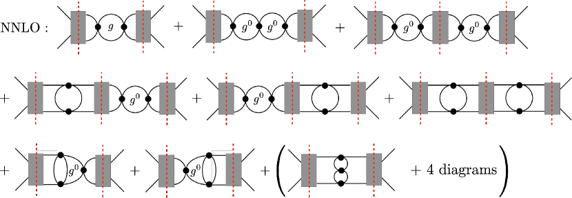
Figure 8: New diagrams contributing to the vertex function for the NNLO determination of the gap.

It is straightforward to evaluate diagram 3a):

$$\Gamma_{3a}\ =\ -\frac{g}{1+g\Pi_{pp}^{(g^{-1})}}\left[1-\frac{g\Pi_{pp}^{(g^{0})}+g\Pi_{pp}^{(g)}}{1+g\Pi_{pp}^{(g^{-1})}}+\left(\frac{g\Pi_{pp}^{(g^{0})}}{1+g\Pi_{pp}^{(g^{-1})}}\right)^{2}\right]\ ,$$ (51)

diagram 3b):

$$\Gamma_{3b}\ =\ \frac{-V^{(g^{2})}}{\left(1+g\Pi_{pp}^{(g^{-1})}\right)^{2}}\left(1-2\frac{g\Pi_{pp}^{(g^{0})}}{1+g\Pi_{pp}^{(g^{-1})}}\right)\ ,$$ (52)

and diagram 3c):

$$\Gamma_{3c}\ =\ \frac{\left(V^{(g^{2})}\right)^{2}\,\Pi_{pp}^{(g^{-1})}}{\left(1+g\Pi_{pp}^{(g^{-1})}\right)^{3}}\ =\ \frac{-\left(V^{(g^{2})}\right)^{2}}{g\left(1+g\Pi_{pp}^{(g^{-1})}\right)^{3}}\ .$$ (53)

In the second equality for $\Gamma_{3c}$ the LO result $\Pi_{pp}^{(g^{-1})}=-1/g$ has been used. The evaluation of diagram 3d) follows similarly to 2b) and gives

$$\Gamma_{3d}\ =\ \frac{-V^{(g^{3})}}{\left(1+g\Pi_{pp}^{(g^{-1})}\right)^{2}}\ ,$$ (54)

where $V^{(g^{3})}$ is determined from the diagrams that contribute to the ${\mathcal{O}}(g^{3})$ component of the 2PI potential, shown in Fig. 9. Diagram 3e) evaluates to

$$\Gamma_{3e}\ =\ 2\frac{g\,{\cal I}\left[\Pi^{(g^{0})}_{pp}\,V^{(g^{2})}\right]}{\left(1+g\Pi_{pp}^{(g^{-1})}\right)^{2}}\ ,$$ (55)

where ${\cal I}\left[\Pi^{(g^{0})}_{pp}\,V^{(g^{2})}\right]$ is the integral of the p-p bubble with ${\cal O}(g^{-1})$ piece subtracted, combined with the ${\cal O}(g^{2})$ component of the 2PI potential. See App. C.2.

The Feynman diagrams in $V^{(g^{3})}$ and ${\cal I}\left[\Pi^{(g^{0})}_{pp}\,V^{(g^{2})}\right]$ are evaluated using a numerical technique originally developed for relativistic quantum field theory. This technique is based on deriving the three-dimensional representation of a Feynman diagram by integrating the energy components of loop integrals analytically [56, 57, 58, 59, 60, 61, 62], performing the singularity analysis and regularization in the integration space of the remaining spatial components [63, 64, 65], and finally numerically performing the regularized integral by direct Monte-Carlo integration (see [66] for a comprehensive review of the method and [67, 68] for recent applications). The results presented below used the VEGAS Python package [69] with nitn=20 and neval=$1\times 10^{11}$, except for the evaluation of $\Pi^{(a)}_{ppph}$ which used neval=$5\times 10^{10}$.

C.1 Computing $V^{(g^{3})}$

Determining the NNLO gap requires computing $V^{(g^{3})}$, the ${\mathcal{O}}(g^{3})$ piece of the 2PI s-wave potential evaluated for external legs on-shell and at the Fermi surface. The diagrams that contribute are shown in Fig. 9, and their evaluation can be simplified by noting that $\Pi_{ppph}^{(c)}$ and $\Pi_{phph}^{(d)}$ are related to $\Pi_{ppph}^{(a)}$ and $\Pi_{phph}^{(b)}$ by ${\bf k}\to-{\bf k}$, and ${\bf k}^{\prime}\to-{\bf k}^{\prime}$.

Figure 9: Diagrams contributing to the 2PI potential at ${\mathcal{O}}(g^{3})$.

Applying the Feynman rules yields:

$$\Pi_{ppph}^{(a)}({\bf k},{\bf k}^{\prime}) = \int\!\frac{d^{4}l}{(2\pi)^{4}}\int\!\frac{d^{4}l^{\prime}}{(2\pi)^{4}}G_{0}(E+l_{0},{\bf l})G_{0}(l_{0}^{\prime}-l_{0},{\bf l}^{\prime}-{\bf l})G_{0}(l_{0}^{\prime},{\bf l}^{\prime}-{\bf k})G_{0}(l_{0}^{\prime},{\bf l}^{\prime}-{\bf k}^{\prime})\ ,$$ (56)

$$\Pi_{phph}^{(b)}({\bf k},{\bf k}^{\prime}) = \int\!\frac{d^{4}l}{(2\pi)^{4}}\int\!\frac{d^{4}l^{\prime}}{(2\pi)^{4}}G_{0}(E+l_{0}-l_{0}^{\prime},{\bf l}-{\bf l}^{\prime}+{\bf k}^{\prime}+{\bf k})G_{0}(l_{0},{\bf l})$$ (57)

$$\mkern 300.0mu\times G_{0}(l_{0}^{\prime},{\bf l}^{\prime}-{\bf k}^{\prime})G_{0}(l_{0}^{\prime},{\bf l}^{\prime}-{\bf k})\ ,$$

$$\Pi_{phph}^{(e)}({\bf k},{\bf k}^{\prime}) = \int\!\frac{d^{4}l}{(2\pi)^{4}}\int\!\frac{d^{4}l^{\prime}}{(2\pi)^{4}}G_{0}(l_{0},{\bf l}+{\bf k}-{\bf k}^{\prime})G_{0}(l_{0},{\bf l})G_{0}(l_{0}^{\prime},{\bf l}^{\prime}+{\bf k}-{\bf k}^{\prime})G_{0}(l_{0}^{\prime},{\bf l}^{\prime})$$ (58)

$$= -\left[\Pi_{ph}({\bf k},{\bf k}^{\prime};0)\right]^{2}\ .$$

The functional dependence on $k_{0}=k_{0}^{\prime}$ has been omitted as both energies are set to $\omega_{k_{F}}$. Putting these together, the ${\cal O}(g^{3})$ contribution to the full 2PI potential is

$$V^{(g^{3})}_{\alpha\beta,\gamma\delta}({\bf k},{\bf k}^{\prime})\ =$$

$$g^{3}\bigg{\{}\delta_{\alpha\delta}\delta_{\beta\gamma}\left[\Pi_{ppph}^{(a)}({\bf k},{\bf k}^{\prime})+\Pi_{ppph}^{(a)}(-{\bf k},-{\bf k}^{\prime})\right]\ -\ \delta_{\alpha\gamma}\delta_{\beta\delta}\left[\Pi_{ppph}^{(a)}({\bf k},-{\bf k}^{\prime})+\Pi_{ppph}^{(a)}(-{\bf k},{\bf k}^{\prime})\right]$$

$$+\ \delta_{\alpha\gamma}\delta_{\beta\delta}\left[\Pi_{phph}^{(b)}({\bf k},{\bf k}^{\prime})+\Pi_{phph}^{(b)}(-{\bf k},-{\bf k}^{\prime})\right]\ -\ \delta_{\alpha\delta}\delta_{\beta\gamma}\left[\Pi_{phph}^{(b)}({\bf k},-{\bf k}^{\prime})+\Pi_{phph}^{(b)}(-{\bf k},{\bf k}^{\prime})\right]$$

$$+\left(\delta_{\alpha\gamma}\delta_{\beta\delta}-\delta_{\alpha\delta}\delta_{\beta\gamma}\right)\left([\Pi_{ph}({\bf k},{\bf k}^{\prime};0)]^{2}+[\Pi_{ph}({\bf k},-{\bf k}^{\prime};0)]^{2}\right)\bigg{\}}$$

$$=g^{3}\bigg{\{}2\delta_{\alpha\delta}\delta_{\beta\gamma}\Pi_{ppph}^{(a)}({\bf k},{\bf k}^{\prime})-2\delta_{\alpha\gamma}\delta_{\beta\delta}\Pi_{ppph}^{(a)}({\bf k},-{\bf k}^{\prime})+2\delta_{\alpha\gamma}\delta_{\beta\delta}\Pi_{phph}^{(b)}({\bf k},{\bf k}^{\prime})-2\delta_{\alpha\delta}\delta_{\beta\gamma}\Pi_{phph}^{(b)}({\bf k},-{\bf k}^{\prime})$$

$$+\left(\delta_{\alpha\gamma}\delta_{\beta\delta}-\delta_{\alpha\delta}\delta_{\beta\gamma}\right)\left([\Pi_{ph}({\bf k},{\bf k}^{\prime};0)]^{2}+[\Pi_{ph}({\bf k},-{\bf k}^{\prime};0)]^{2}\right)\bigg{\}}$$

$$\ \stackrel{{\scriptstyle\text{s-wave}}}{{=}}2g^{3}\left(\delta_{\alpha\gamma}\delta_{\beta\delta}-\delta_{\alpha\delta}\delta_{\beta\gamma}\right)\left([\Pi_{ph}({\bf k},{\bf k}^{\prime};0)]^{2}\ -\ \Pi_{ppph}^{(a)}({\bf k},{\bf k}^{\prime})\ +\ \Pi_{phph}^{(b)}({\bf k},{\bf k}^{\prime})\right)\ ,$$ (59)

where the third equality has used the fact that the s-wave projection is invariant under ${\bf k}^{\prime}\to-{\bf k}^{\prime}$. The spin factors are determined from the dotted-line decomposition shown in Fig. 10.

To determine $V^{(g^{3})}$ the potential has to be projected onto the s-wave. For numerical evaluation it is convenient to do this by fixing ${\bf k}=k_{F}\hat{z}$ and integrating over ${\bf k}^{\prime}$ in the x-z plane i.e. ${\bf k}^{\prime}=k_{F}(\sin{\theta},0,\cos{\theta})^{T}$. For example,

$$V^{g^{3}}\ =\ g^{3}\int_{0}^{\pi}\!d\theta\sin{\theta}\left[\Pi(k_{F}\hat{z},k_{F}(\sin{\theta},0,\cos{\theta})^{T})\right]\ .$$ (60)

The final result is

$$V^{(g^{3})}\ =g^{3}\int_{0}^{\pi}\!d\theta\,\sin{\theta}\left(-\Pi^{(a)}_{ppph}({\bf k},{\bf k}^{\prime})\ +\ \Pi^{(b)}_{phph}({\bf k},{\bf k}^{\prime})\ +\ \Pi_{ph}({\bf k},{\bf k}^{\prime})^{2}\right)$$

$$=g\frac{g^{2}M^{2}k_{F}^{2}}{4\pi^{4}}\left(0.972041(15)\ -\ 0.0418477(64)\ +\ \frac{1}{4}\left[1+\frac{7}{2}\zeta(3)\right]\right)$$

$$=2.231993(16)\,g\,\lambda^{2}\ .$$ (61)

The evaluation of the individual terms is detailed below.

First, consider evaluating $\Pi_{ppph}^{(a)}({\bf k},{\bf k}^{\prime})$. It is convenient to define ${\bf q_{1}}={\bf l}^{\prime}-{\bf k}^{\prime}$, ${\bf q_{2}}={\bf l}^{\prime}-{\bf k}$ and ${\bf q_{3}}={\bf l}^{\prime}-{\bf l}$. Performing the $l_{0}$ and $l_{0}^{\prime}$ integrals one finds

$$\Pi^{(a)}_{ppph}({\bf k},{\bf k}^{\prime})\ =\ \int\!\frac{d^{4}l^{\prime}}{(2\pi)^{4}}\int\!\frac{d^{4}l}{(2\pi)^{4}}G_{0}(l_{0}^{\prime},{\bf q}_{1})G_{0}(l_{0}^{\prime},{\bf q}_{2})G_{0}(E+l_{0},{\bf l})G_{0}(l_{0}^{\prime}-l_{0},{\bf q}_{3})$$

$$=\int\!\frac{d^{3}{\bf l}^{\prime}}{(2\pi)^{3}}\int\!\frac{d^{3}{\bf l}}{(2\pi)^{3}}\Bigg{\{}\frac{\theta(k_{F}-q_{3})-\theta(l-k_{F})}{\omega_{q_{1}}-\omega_{q_{2}}}\left(\frac{\theta(k_{F}-q_{2})}{\omega_{q_{2}}+E-\omega_{l}-\omega_{q_{3}}}-\frac{\theta(k_{F}-q_{1})}{\omega_{q_{1}}+E-\omega_{l}-\omega_{q_{3}}}\right)$$

$$-\theta(k_{F}-l)\theta(k_{F}-q_{3})\left[\frac{1}{(-E+\omega_{l}+\omega_{q_{3}}-\omega_{q_{1}})(-E+\omega_{l}+\omega_{q_{3}}-\omega_{q_{2}})}\right]\Bigg{\}}\ .$$ (62)

In the second line, the $(i\epsilon)$s can be safely dropped because the integrand does not have non-integrable singularities (and therefore there is no imaginary component). This is explicitly verified at a mathematical level by a simple power-counting procedure, and at a practical level by performing the numerical integration, which gives a finite result with no need for a principal value prescription. The terms with $\theta(l-k_{F})$ are UV divergent for $l\to\infty$, and can be subtracted and evaluated analytically in the PDS scheme. To preserve the IR structure only the leading UV divergences are subtracted,

$$\int\!\frac{d^{3}{\bf l}^{\prime}}{(2\pi)^{3}}\int\!\frac{d^{3}{\bf l}}{(2\pi)^{3}}\frac{-\theta(l-k_{F})}{\omega_{q_{1}}-\omega_{q_{2}}}\left(\frac{\theta(k_{F}-q_{2})}{\omega_{q_{2}}+E-\omega_{l}-\omega_{q_{3}}}-\frac{\theta(k_{F}-q_{1})}{\omega_{q_{1}}+E-\omega_{l}-\omega_{q_{3}}}\right)$$

$$=\int\!\frac{d^{3}{\bf l}^{\prime}}{(2\pi)^{3}}\int\!\frac{d^{3}{\bf l}}{(2\pi)^{3}}\frac{-\theta(l-k_{F})}{2\omega_{l}}\left(1+\frac{{\bf l}\cdot{\bf l}^{\prime}}{l^{2}}+\mathcal{O}(l^{-2})\right)\left[\frac{\theta(k_{F}-q_{1})-\theta(k_{F}-q_{2})}{\omega_{q_{1}}-\omega_{q_{2}}}\right]$$

$$=\frac{M\mu}{4\pi}\Pi_{ph}(q)-\frac{Mk_{F}}{2\pi^{2}}\Pi_{ph}(q)\ .$$ (63)

Notice that the ${\bf l}\cdot{\bf l}^{\prime}$ term is only zero at the integrated level, and therefore needs to be kept so that the integrand is UV finite. Explicitly,

$$\Pi^{(a)}_{ppph}({\bf k},{\bf k}^{\prime})=\left(\frac{M\mu}{4\pi}-\frac{Mk_{F}}{2\pi^{2}}\right)\Pi_{ph}(q)$$

$$+\int\!\frac{d^{3}{\bf l}^{\prime}}{(2\pi)^{3}}\int\!\frac{d^{3}{\bf l}}{(2\pi)^{3}}\Bigg{\{}\frac{\theta(k_{F}-q_{3})-\theta(l-k_{F})}{\omega_{q_{1}}-\omega_{q_{2}}}\left(\frac{\theta(k_{F}-q_{2})}{\omega_{q_{2}}+E-\omega_{l}-\omega_{q_{3}}}-\frac{\theta(k_{F}-q_{1})}{\omega_{q_{1}}+E-\omega_{l}-\omega_{q_{3}}}\right)$$

$$-\theta(k_{F}-l)\theta(k_{F}-q_{3})\left[\frac{1}{(-E+\omega_{l}+\omega_{q_{3}}-\omega_{q_{1}})(-E+\omega_{l}+\omega_{q_{3}}-\omega_{q_{2}})}\right]$$

$$+\frac{\theta(l-k_{F})}{2\omega_{l}}\left(1+\frac{{\bf l}\cdot{\bf l}^{\prime}}{l^{2}}\right)\left[\frac{\theta(k_{F}-q_{1})-\theta(k_{F}-q_{2})}{\omega_{q_{1}}-\omega_{q_{2}}}\right]\Bigg{\}}\ ,$$ (64)

where the integral in curly braces is evaluated with Monte Carlo integration.

To verify renormalizability, it can be shown that all $\mu$-dependence cancels at this order. The $\mu$-dependence in $V^{(g^{3})}$ coming from $\Pi_{pphh}^{(a)}$ is,

$$V^{(g^{3})}_{\alpha,\beta,\gamma\delta}({\bf k},{\bf k}^{\prime};\omega)[\mu]\ =\ 2g(\mu)^{3}\frac{M\mu}{4\pi}\left(\Pi_{ph}({\bf k},{\bf k}^{\prime};\omega)\delta_{\alpha\delta}\delta_{\beta\gamma}\ -\ \Pi_{ph}({\bf k},-{\bf k}^{\prime};\omega)\delta_{\alpha\gamma}\delta_{\beta\delta}\right)$$

$$=\left(\frac{4\pi a}{M}\right)^{2}\left(2a\mu\ +\ {\mathcal{O}}[(a\mu)^{2}]\right)\left(\Pi_{ph}({\bf k},{\bf k}^{\prime};\omega)\delta_{\alpha\delta}\delta_{\beta\gamma}\ -\ \Pi_{ph}({\bf k},-{\bf k}^{\prime};\omega)\delta_{\alpha\gamma}\delta_{\beta\delta}\right)\ ,$$ (65)

where the PDS coupling has been expanded in powers of $(a\mu)$ using Eq. (11). This $\mu$-dependence must cancel in physical quantities, for example in the NNLO gap equation, Eq. (32). Only the sum $\left[V^{(g^{2})}+V^{(g^{3})}\right]$ enters and the $\mu$-dependence of $V^{(g^{2})}$

$$V^{(g^{2})}_{\alpha\beta,\gamma\delta}({\bf k},{\bf k}^{\prime};\omega)[\mu]\ =\ g(\mu)^{2}\left(\Pi_{ph}({\bf k},-{\bf k}^{\prime};\omega)\delta_{\alpha\gamma}\delta_{\beta\delta}-\Pi_{ph}({\bf k},{\bf k}^{\prime};\omega)\delta_{\alpha\delta}\delta_{\beta\gamma}\right)$$

$$=\ \left(\frac{4\pi a}{M}\right)^{2}\left(1\ -\ 2a\mu\ +\ {\mathcal{O}}([a\mu]^{2})\right)\left(\Pi_{ph}({\bf k},{\bf k}^{\prime};\omega)\delta_{\alpha\delta}\delta_{\beta\gamma}-\Pi_{ph}({\bf k},-{\bf k}^{\prime};\omega)\delta_{\alpha\gamma}\delta_{\beta\delta}\right)\ ,$$ (66)

removes all $\mu$-dependence from the NNLO gap equation.

Next is the evaluation of $\Pi^{(b)}_{phph}({\bf k},{\bf k}^{\prime})$. Defining ${\bf q_{1}}={\bf l}^{\prime}-{\bf k}^{\prime}$, ${\bf q_{2}}={\bf l}^{\prime}-{\bf k}$ and ${\bf q_{3}}={\bf l}-{\bf l}^{\prime}+{\bf k}+{\bf k}^{\prime}$, and performing the $l_{0}$ and $l_{0}^{\prime}$ integrals gives,

$$\Pi^{(b)}_{phph}({\bf k},{\bf k}^{\prime})\ =\ \int\!\frac{d^{4}l^{\prime}}{(2\pi)^{4}}\int\!\frac{d^{4}l}{(2\pi)^{4}}G_{0}(l_{0}^{\prime},{\bf q}_{1})G_{0}(l_{0}^{\prime},{\bf q}_{2})G_{0}(l_{0},{\bf l})G_{0}(E+l_{0}-l_{0}^{\prime},{\bf q}_{3})$$

$$=\int\!\frac{d^{3}{\bf l}^{\prime}}{(2\pi)^{3}}\int\!\frac{d^{3}{\bf l}}{(2\pi)^{3}}\Bigg{\{}\frac{\theta(k_{F}-l)-\theta(k_{F}-q_{3})}{\omega_{q_{1}}-\omega_{q_{2}}}\left[\frac{\theta(q_{1}-k_{F})}{-\omega_{q_{1}}+E+\omega_{l}-\omega_{q_{3}}}\ -\ \frac{\theta(q_{2}-k_{F})}{-\omega_{q_{2}}+E+\omega_{l}-\omega_{q_{3}}}\right]$$

$$+\ \theta(l-k_{F})\theta(k_{F}-q_{3})\left[\frac{1}{(E+\omega_{l}-\omega_{q_{3}}-\omega_{q_{1}})(E+\omega_{l}-\omega_{q_{3}}-\omega_{q_{2}})}\right]\Bigg{\}}\ .$$ (67)

This expression has no non-integrable singularities, and the contribution to the s-wave potential can be directly computed using Eq. (60).

As a check, the potential can be projected onto the p-wave, and compared to Eq. (18) in Ref. [39]. The p-wave potential is

$$V^{g^{3}}_{\ell=1}\ =\ g^{3}\int_{0}^{\pi}\!d\theta\sin{\theta}\cos{\theta}\left[\Pi^{(a)}_{ppph}({\bf k},{\bf k}^{\prime})\ +\ \Pi^{(b)}_{phph}({\bf k},{\bf k}^{\prime})\right]$$

$$=-0.3313(30)g\lambda^{2}$$ (68)

in agreement with $V^{g^{3}}_{\ell=1}=-0.33g\lambda^{2}$ quoted in Ref. [39]. Note that $\Pi^{(e)}_{phph}=-(\Pi_{ph})^{2}$ does not contribute for odd partial waves, and that ${\bf k}^{\prime}\to-{\bf k}^{\prime}$ causes a change of sign (and hence no minus in front of $\Pi^{(a)}$).

C.2 Computing $\Gamma_{3e}$

Determining the NNLO gap requires computing diagram 3e) in Fig. 6,

$$\Gamma_{3e}\ =\ \frac{2g^{3}}{\left[1+g\Pi_{pp}^{(g^{-1})}\right]^{2}}\int\!\frac{d^{4}l}{(2\pi)^{4}}\int\!\frac{d^{4}l^{\prime}}{(2\pi)^{4}}G_{0}({\bf l},l_{0}+E)G_{0}(-{\bf l},-l_{0}+E)G(l_{0}^{\prime},{\bf l}^{\prime})G(l_{0}^{\prime}-l_{0},q_{3})$$

$$\equiv\frac{2g}{\left[1+g\Pi_{pp}^{(g^{-1})}\right]^{2}}\,{\cal I}\left[\Pi^{(g^{0})}_{pp}\,V^{(g^{2})}\right],$$ (69)

where ${\bf q}_{3}={\bf l}^{\prime}+{\bf k}^{\prime}-{\bf l}$ with ${\bf k}^{\prime}$ the outgoing momentum. Since, the particle-particle bubbles do not mix partial waves, the final result will not depend on ${\bf k}^{\prime}$, but intermediate results will. Performing the two energy integrals gives,

$${\cal I}\left[\Pi^{(g^{0})}_{pp}\,V^{(g^{2})}\right]\ =\ g^{2}\int\!\frac{d^{3}{\bf l}}{(2\pi)^{3}}\int\!\frac{d^{3}{\bf l}^{\prime}}{(2\pi)^{3}}\Bigg{\{}\frac{\theta(l-k_{F})\theta(l^{\prime}-k_{F})\theta(k_{F}-q_{3})}{(E+\omega_{l^{\prime}}-\omega_{q_{3}}-\omega_{l}+i\epsilon)(E+\omega_{q_{3}}-\omega_{l^{\prime}}-\omega_{l}+i\epsilon)}$$

$$+\frac{\theta(k_{F}-l)\theta(l^{\prime}-k_{F})\theta(k_{F}-q_{3})}{(E+\omega_{l^{\prime}}-\omega_{q_{3}}-\omega_{l}-i\epsilon)(E+\omega_{q_{3}}-\omega_{l^{\prime}}-\omega_{l}-i\epsilon)}+\frac{\theta(l-k_{F})\left(\theta(k_{F}-l^{\prime})-\theta(k_{F}-q_{3})\right)}{(2E-2\omega_{l}+i\epsilon)(\omega_{l^{\prime}}+E-\omega_{l}-\omega_{q_{3}}+i\epsilon)}$$

$$-\frac{\theta(k_{F}-l)\left(\theta(k_{F}-l^{\prime})-\theta(k_{F}-q_{3})\right)}{(2E-2\omega_{l}-i\epsilon)(-E+\omega_{l^{\prime}}+\omega_{l}-\omega_{q_{3}}+i\epsilon)}\Bigg{\}}$$

$$=g^{2}\int\!\frac{d^{3}{\bf l}}{(2\pi)^{3}}\int\!\frac{d^{3}{\bf l}^{\prime}}{(2\pi)^{3}}\Bigg{\{}\frac{\theta(l^{\prime}-k_{F})\theta(k_{F}-q_{3})}{(E+\omega_{l^{\prime}}-\omega_{q_{3}}-\omega_{l})(E+\omega_{q_{3}}-\omega_{l^{\prime}}-\omega_{l})}$$

$$+\frac{\theta(l-k_{F})\left(\theta(k_{F}-l^{\prime})-\theta(k_{F}-q_{3})\right)}{(2E-2\omega_{l}+i\epsilon)(\omega_{l^{\prime}}+E-\omega_{l}-\omega_{q_{3}})}-\frac{\theta(k_{F}-l)\left(\theta(k_{F}-l^{\prime})-\theta(k_{F}-q_{3})\right)}{(2E-2\omega_{l}-i\epsilon)(-E+\omega_{l^{\prime}}+\omega_{l}-\omega_{q_{3}})}\Bigg{\}}$$ (70)

where in the second equality the $(i\epsilon)$s which regulate integrable singularities have been dropped. The only non-integrable singularity is at $2E=2\omega_{l}$, corresponding to the BCS singularity in the $\Pi_{pp}$ sub-loop. This can be regulated by subtracting and adding back a counter-term where $\omega_{l}=E$ in all non-singular quantities,

$$\int\!\frac{d^{3}{\bf l}}{(2\pi)^{3}}\int\!\frac{d^{3}{\bf l}^{\prime}}{(2\pi)^{3}}\frac{\left(\theta(k_{F}-l^{\prime})-\theta(k_{F}-\bar{q}_{3})\right)\left(\theta(\Lambda-l)\theta(l-k_{F})-\theta(k_{F}-l)\right)}{(\omega_{l^{\prime}}-\omega_{\bar{q}_{3}})(2E-2\omega_{l})}$$

$$=\int\!\frac{d^{3}{\bf l}^{\prime}}{(2\pi)^{3}}\int\!\frac{d\Omega_{l}}{(2\pi)^{3}}\frac{\left(\theta(k_{F}-l^{\prime})-\theta(k_{F}-\bar{q}_{3})\right)}{(\omega_{l^{\prime}}-\omega_{\bar{q}_{3}})}\left[\int_{0}^{\Lambda}\!dl\frac{l^{2}}{2E-2\omega_{l}}-2\int_{0}^{k_{F}}\!dl\frac{l^{2}}{2E-2\omega_{l}}\right]$$

$$=-\frac{k_{F}M}{4\pi^{2}}\int_{0}^{2}\!dq\Pi_{ph}(q)\left[-\frac{\Lambda}{k_{F}}+\coth^{-1}\left(\frac{\Lambda}{k_{F}}\right)-2(\log{2}-1)+\log\left(\frac{\Delta}{2\omega_{k_{F}}}\right)\right]$$

$$=-\frac{M^{2}k_{F}^{2}}{12\pi^{4}}(1+2\log{2})\left[-\frac{1}{3}(1+2\log{2})-\frac{\Lambda}{k_{F}}+\coth^{-1}\left(\frac{\Lambda}{k_{F}}\right)\right]$$ (71)

where $\overline{q}_{3}={\bf l}^{\prime}+{\bf k}^{\prime}-k_{F}{\bf l}/l$ is $q_{3}$ with $l=k_{F}$. This decouples the singular integration over $l$ in the two loops. Taking $q_{3}\to\bar{q}_{3}$ changes the UV behavior of the $\int\!d^{3}l$ integration, and has been regulated with the $\theta(\Lambda-l)$. As this quantity is subtracted and added back in, the final result will not depend on $\Lambda$. In the fourth line, the ${\cal O}(g^{0})$ expression for $\log{\left({\Delta}/(2\omega_{k_{F}})\right)}$ has been substituted since the ${\cal O}(g^{-1})$ piece has already been counted in $\Gamma_{3b}$. Explicitly,

$${\cal I}\left[\Pi^{(g^{0})}_{pp}\,V^{(g^{2})}\right]\ =\ g^{2}\int\!\frac{d^{3}{\bf l}}{(2\pi)^{3}}\int\!\frac{d^{3}{\bf l}^{\prime}}{(2\pi)^{3}}\Bigg{\{}\frac{\theta(l^{\prime}-k_{F})\theta(k_{F}-q_{3})}{(E+\omega_{l^{\prime}}-\omega_{q_{3}}-\omega_{l})(E+\omega_{q_{3}}-\omega_{l^{\prime}}-\omega_{l})}$$

$$+\frac{\theta(l-k_{F})\left(\theta(k_{F}-l^{\prime})-\theta(k_{F}-q_{3})\right)}{(2E-2\omega_{l})(\omega_{l^{\prime}}+E-\omega_{l}-\omega_{q_{3}})}-\frac{\theta(k_{F}-l)\left(\theta(k_{F}-l^{\prime})-\theta(k_{F}-q_{3})\right)}{(2E-2\omega_{l})(-E+\omega_{l^{\prime}}+\omega_{l}-\omega_{q_{3}})}$$

$$-\frac{\left(\theta(k_{F}-l^{\prime})-\theta(k_{F}-\bar{q}_{3})\right)\left(\theta(\Lambda-l)\theta(l-k_{F})-\theta(k_{F}-l)\right)}{(\omega_{l^{\prime}}-\omega_{\bar{q}_{3}})(2E-2\omega_{l})}\Bigg{\}}$$

$$-\frac{M^{2}k_{F}^{2}}{12\pi^{4}}(1+2\log{2})\left[-\frac{1}{3}(1+2\log{2})-\frac{\Lambda}{k_{F}}+\coth^{-1}\left(\frac{\Lambda}{k_{F}}\right)\right]$$ (72)

where the expression in curly braces is evaluated with Monte Carlo. The final result does not depend on ${\bf k}^{\prime}$ or $\Lambda$, and is found to be

$${\cal I}\left[\Pi^{(g^{0})}_{pp}\,V^{(g^{2})}\right]\ =\ 0.917746(98)\,\lambda^{2}\ .$$ (73)

Figure 10: Spin contractions for $V^{(g^{3})}$.

References

- Dean and Hjorth-Jensen [2003] D. J. Dean and M. Hjorth-Jensen, Pairing in nuclear systems: From neutron stars to finite nuclei, Rev. Mod. Phys. 75, 607 (2003), arXiv:nucl-th/0210033 .
- Kanada-En’yo et al. [2009] Y. Kanada-En’yo, N. Hinohara, T. Suhara, and P. Schuck, Dineutron correlations in quasi two-dimensional systems in a simplified model and possible relation to neutron-rich nuclei, Phys. Rev. C 79, 054305 (2009), arXiv:0902.3717 [nucl-th] .
- Page et al. [2011] D. Page, M. Prakash, J. M. Lattimer, and A. W. Steiner, Rapid Cooling of the Neutron Star in Cassiopeia A Triggered by Neutron Superfluidity in Dense Matter, Phys. Rev. Lett. 106, 081101 (2011), arXiv:1011.6142 [astro-ph.HE] .
- Watanabe and Pethick [2017] G. Watanabe and C. J. Pethick, Superfluid Density of Neutrons in the Inner Crust of Neutron Stars: New Life for Pulsar Glitch Models, Phys. Rev. Lett. 119, 062701 (2017), arXiv:1704.08859 [nucl-th] .
- Chamel [2017] N. Chamel, Superfluidity and Superconductivity in Neutron Stars, J. Astrophys. Astron. 38, 43 (2017), arXiv:1709.07288 [astro-ph.HE] .
- Haskell and Sedrakian [2018] B. Haskell and A. Sedrakian, Superfluidity and Superconductivity in Neutron Stars, Astrophys. Space Sci. Libr. 457, 401 (2018), arXiv:1709.10340 [astro-ph.HE] .
- Gezerlis et al. [2014] A. Gezerlis, C. J. Pethick, and A. Schwenk, 580Pairing and superfluidity of nucleons in neutron stars, in Novel Superfluids: Volume 2 (Oxford University Press, 2014) https://academic.oup.com/book/0/chapter/367245219/chapter-pdf/45154249/acprof-9780198719267-chapter-11.pdf .
- Ramanan and Urban [2021] S. Ramanan and M. Urban, Pairing in pure neutron matter, Eur. Phys. J. ST 230, 567 (2021), arXiv:2010.09632 [nucl-th] .
- Ding et al. [2016] D. Ding, A. Rios, H. Dussan, W. H. Dickhoff, S. J. Witte, A. Polls, and A. Carbone, Pairing in high-density neutron matter including short- and long-range correlations, Phys. Rev. C 94, 025802 (2016), [Addendum: Phys.Rev.C 94, 029901 (2016)], arXiv:1601.01600 [nucl-th] .
- Pavlou et al. [2017] G. E. Pavlou, E. Mavrommatis, C. Moustakidis, and J. W. Clark, Microscopic Study of Superfluidity in Dilute Neutron Matter, Eur. Phys. J. A 53, 96 (2017), arXiv:1612.02188 [nucl-th] .
- Krotscheck and Wang [2022] E. Krotscheck and J. Wang, Variational and parquet-diagram calculations for neutron matter. IV. Spin-orbit interactions and linear response, Phys. Rev. C 105, 034345 (2022), arXiv:2111.12051 [nucl-th] .
- Cao et al. [2006] L. G. Cao, U. Lombardo, and P. Schuck, Screening effects in superfluid nuclear and neutron matter within Brueckner theory, Phys. Rev. C 74, 064301 (2006), arXiv:nucl-th/0608005 .
- Shen et al. [2003] C. Shen, U. Lombardo, and P. Schuck, Screening effects on S(0)-1 pairing in neutron matter, Phys. Rev. C 67, 061302 (2003), arXiv:nucl-th/0212027 .
- Schwenk et al. [2003] A. Schwenk, B. Friman, and G. E. Brown, Renormalization group approach to neutron matter: Quasiparticle interactions, superfluid gaps and the equation of state, Nucl. Phys. A 713, 191 (2003), arXiv:nucl-th/0207004 .
- Wambach et al. [1993] J. Wambach, T. L. Ainsworth, and D. Pines, Quasiparticle interactions in neutron matter for applications in neutron stars, Nucl. Phys. A 555, 128 (1993).
- Sedrakian et al. [2003] A. Sedrakian, T. T. S. Kuo, H. Muther, and P. Schuck, Pairing in nuclear systems with effective Gogny and V(low-k) interactions, Phys. Lett. B 576, 68 (2003), arXiv:nucl-th/0308068 .
- Urban and Ramanan [2020] M. Urban and S. Ramanan, Neutron pairing with medium polarization beyond the Landau approximation, Phys. Rev. C 101, 035803 (2020), arXiv:1911.10772 [nucl-th] .
- Gandolfi et al. [2022] S. Gandolfi, G. Palkanoglou, J. Carlson, A. Gezerlis, and K. E. Schmidt, The 1s0 pairing gap in neutron matter, Condensed Matter 7, 19 (2022).
- Carlson et al. [2012] J. Carlson, S. Gandolfi, and A. Gezerlis, Quantum Monte Carlo approaches to nuclear and atomic physics, PTEP 2012, 01A209 (2012), arXiv:1210.6659 [nucl-th] .
- Gezerlis and Carlson [2010] A. Gezerlis and J. Carlson, Low-density neutron matter, Phys. Rev. C 81, 025803 (2010), arXiv:0911.3907 [nucl-th] .
- Gandolfi et al. [2008] S. Gandolfi, A. Y. Illarionov, S. Fantoni, F. Pederiva, and K. E. Schmidt, Equation of state of superfluid neutron matter and the calculation of S(0)-1 pairing gap, Phys. Rev. Lett. 101, 132501 (2008), arXiv:0805.2513 [nucl-th] .
- Bardeen et al. [1957] J. Bardeen, L. N. Cooper, and J. R. Schrieffer, Theory of superconductivity, Phys. Rev. 108, 1175 (1957).
- Polchinski [1992] J. Polchinski, Effective field theory and the Fermi surface, in Theoretical Advanced Study Institute (TASI 92): From Black Holes and Strings to Particles (1992) pp. 0235–276, arXiv:hep-th/9210046 .
- Shankar [1994] R. Shankar, Renormalization-group approach to interacting fermions, Rev. Mod. Phys. 66, 129 (1994).
- Papenbrock and Bertsch [1999] T. Papenbrock and G. F. Bertsch, Pairing in low density Fermi gases, Phys. Rev. C 59, 2052 (1999), arXiv:nucl-th/9811077 .
- Marini et al. [1998] M. Marini, F. Pistolesi, and G. C. Strinati, Evolution from bcs superconductivity to bose condensation: analytic results for the crossover in three dimensions, The European Physical Journal B - Condensed Matter and Complex Systems 1, 151 (1998).
- Furnstahl et al. [2007] R. J. Furnstahl, H. W. Hammer, and S. J. Puglia, Effective Field Theory for Dilute Fermions with Pairing, Annals Phys. 322, 2703 (2007), arXiv:nucl-th/0612086 .
- Schäfer [2012] T. Schäfer, Effective Theories of Dense and Very Dense Matter, Lect. Notes Phys. 852, 193 (2012), arXiv:nucl-th/0609075 .
- O’Hara et al. [2002] K. M. O’Hara, S. L. Hemmer, M. E. Gehm, S. R. Granade, and J. E. Thomas, Observation of a strongly interacting degenerate fermi gas of atoms, Science 298, 2179–2182 (2002).
- Bourdel et al. [2003] T. Bourdel, J. Cubizolles, L. Khaykovich, K. M. F. Magalhães, S. J. J. M. F. Kokkelmans, G. V. Shlyapnikov, and C. Salomon, Measurement of the interaction energy near a feshbach resonance in a fermi gas, Phys. Rev. Lett. 91, 020402 (2003).
- Giorgini et al. [2008] S. Giorgini, L. P. Pitaevskii, and S. Stringari, Theory of ultracold atomic Fermi gases, Rev. Mod. Phys. 80, 1215 (2008), arXiv:0706.3360 [cond-mat.other] .
- Chang et al. [2004] S. Y. Chang, V. R. Pandharipande, J. Carlson, and K. E. Schmidt, Quantum Monte Carlo Studies of Superfluid Fermi Gases, Phys. Rev. A 70, 043602 (2004), arXiv:physics/0404115 .
- Gor’kov and Melik-Barkhudarov [1961] L. P. Gor’kov and T. K. Melik-Barkhudarov, Contribution to the theory of superfluidity in an imperfect fermi gas, Soviet Physics JETP 13, 1018 (1961).
- Kohn and Luttinger [1965] W. Kohn and J. M. Luttinger, New Mechanism for Superconductivity, Phys. Rev. Lett. 15, 524 (1965).
- Baranov et al. [1992] M. A. Baranov, A. V. Chubukov, and M. Y. Kagan, Superconductivity and Superfluidity in Fermi Systems with Repulsive Interactions, International Journal of Modern Physics B 6, 2471 (1992).
- Efremov et al. [2000a] D. V. Efremov, M. S. Mar’enko, M. A. Baranov, and M. Y. Kagan, Superfluid transition temperature in a fermi gas with repulsion allowing for higher orders of perturbation theory, Journal of Experimental and Theoretical Physics 90, 861 (2000a).
- Chubukov [1993] A. V. Chubukov, Kohn-luttinger effect and the instability of a two-dimensional repulsive fermi liquid at t=0, Phys. Rev. B 48, 1097 (1993).
- Landau et al. [1980] L. Landau, E. Lifshitz, and L. Pitaevskii, Course of Theoretical Physics: Statistical Physics, Part 2 : by E.M. Lifshitz and L.P. Pitaevskii, v. 9 (1980).
- Efremov et al. [2000b] D. V. Efremov, M. S. Mar’enko, M. A. Baranov, and M. Y. Kagan, Superfluid transition temperature in a fermi gas with repulsion allowing for higher orders of perturbation theory, Journal of Experimental and Theoretical Physics 90, 861 (2000b).
- Kaplan et al. [1998a] D. B. Kaplan, M. J. Savage, and M. B. Wise, A New expansion for nucleon-nucleon interactions, Phys. Lett. B 424, 390 (1998a), arXiv:nucl-th/9801034 .
- Kaplan et al. [1998b] D. B. Kaplan, M. J. Savage, and M. B. Wise, Two nucleon systems from effective field theory, Nucl. Phys. B 534, 329 (1998b), arXiv:nucl-th/9802075 .
- Kohn and Luttinger [1960] W. Kohn and J. M. Luttinger, Ground-State Energy of a Many-Fermion System, Phys. Rev. 118, 41 (1960).
- Luttinger and Ward [1960] J. M. Luttinger and J. C. Ward, Ground state energy of a many fermion system. 2., Phys. Rev. 118, 1417 (1960).
- Fetter and Walecka [1971] A. L. Fetter and J. D. Walecka, Quantum Theory of Many-Particle Systems (McGraw-Hill, Boston, 1971).
- Hammer and Furnstahl [2000] H. W. Hammer and R. J. Furnstahl, Effective field theory for dilute Fermi systems, Nucl. Phys. A 678, 277 (2000), arXiv:nucl-th/0004043 .
- Kaiser [2011] N. Kaiser, Resummation of fermionic in-medium ladder diagrams to all orders, Nucl. Phys. A 860, 41 (2011), arXiv:1102.2154 [nucl-th] .
- Abrikosov et al. [1964] A. A. Abrikosov, L. P. Gorkov, I. E. Dzyaloshinski, R. A. Silverman, and G. H. Weiss, Methods of Quantum Field Theory in Statistical Physics, Physics Today 17, 78 (1964), https://pubs.aip.org/physicstoday/article-pdf/17/4/78/8261542/78_1_online.pdf .
- Maiti and Chubukov [2013] S. Maiti and A. V. Chubukov, Superconductivity from repulsive interaction, in AIP Conference Proceedings (AIP, 2013).
- de Swart et al. [1995] J. J. de Swart, C. P. F. Terheggen, and V. G. J. Stoks, The low-energy n p scattering parameters and the deuteron, in 3rd International Symposium on Dubna Deuteron 95 (1995) arXiv:nucl-th/9509032 [nucl-th] .
- Platter et al. [2003] L. Platter, H. W. Hammer, and U. G. Meissner, Quasiparticle properties in effective field theory, Nucl. Phys. A 714, 250 (2003), arXiv:nucl-th/0208057 .
- Beane and Savage [2001] S. R. Beane and M. J. Savage, Rearranging pionless effective field theory, Nucl. Phys. A 694, 511 (2001), arXiv:nucl-th/0011067 .
- Schwenk and Pethick [2005] A. Schwenk and C. J. Pethick, Resonant Fermi gases with a large effective range, Phys. Rev. Lett. 95, 160401 (2005), arXiv:nucl-th/0506042 .
- Beane and Farrell [2022] S. R. Beane and R. C. Farrell, Symmetries of the Nucleon–Nucleon S-Matrix and Effective Field Theory Expansions, Few Body Syst. 63, 45 (2022), arXiv:2112.05800 [nucl-th] .
- Peng et al. [2022] R. Peng, S. Lyu, S. König, and B. Long, Constructing chiral effective field theory around unnatural leading-order interactions, Phys. Rev. C 105, 054002 (2022), arXiv:2112.00947 [nucl-th] .
- Birse et al. [2005] M. C. Birse, B. Krippa, J. A. McGovern, and N. R. Walet, Pairing in many-fermion systems: An Exact renormalisation group treatment, Phys. Lett. B 605, 287 (2005), arXiv:hep-ph/0406249 .
- Catani et al. [2008] S. Catani, T. Gleisberg, F. Krauss, G. Rodrigo, and J.-C. Winter, From loops to trees by-passing Feynman’s theorem, JHEP 09, 065, arXiv:0804.3170 [hep-ph] .
- Bierenbaum et al. [2010] I. Bierenbaum, S. Catani, P. Draggiotis, and G. Rodrigo, A tree-loop duality relation at two loops and beyond, JHEP 10, 073, arXiv:1007.0194 [hep-ph] .
- Runkel et al. [2019] R. Runkel, Z. Szőr, J. P. Vesga, and S. Weinzierl, Causality and loop-tree duality at higher loops, Phys. Rev. Lett. 122, 111603 (2019), [Erratum: Phys.Rev.Lett. 123, 059902 (2019)], arXiv:1902.02135 [hep-ph] .
- Capatti et al. [2019] Z. Capatti, V. Hirschi, D. Kermanschah, and B. Ruijl, Loop-Tree Duality for Multiloop Numerical Integration, Phys. Rev. Lett. 123, 151602 (2019), arXiv:1906.06138 [hep-ph] .
- Capatti [2023a] Z. Capatti, Exposing the threshold structure of loop integrals, Phys. Rev. D 107, L051902 (2023a), arXiv:2211.09653 [hep-th] .
- Jesús Aguilera-Verdugo et al. [2021] J. Jesús Aguilera-Verdugo, R. J. Hernández-Pinto, G. Rodrigo, G. F. R. Sborlini, and W. J. Torres Bobadilla, Mathematical properties of nested residues and their application to multi-loop scattering amplitudes, JHEP 02, 112, arXiv:2010.12971 [hep-ph] .
- Sborlini [2021] G. F. R. Sborlini, Geometrical approach to causality in multiloop amplitudes, Physical Review D 104, 10.1103/physrevd.104.036014 (2021).
- Capatti et al. [2020] Z. Capatti, V. Hirschi, D. Kermanschah, A. Pelloni, and B. Ruijl, Numerical Loop-Tree Duality: contour deformation and subtraction, JHEP 04, 096, arXiv:1912.09291 [hep-ph] .
- Kermanschah [2022] D. Kermanschah, Numerical integration of loop integrals through local cancellation of threshold singularities, JHEP 01, 151, arXiv:2110.06869 [hep-ph] .
- Capatti et al. [2022] Z. Capatti, V. Hirschi, and B. Ruijl, Local unitarity: cutting raised propagators and localising renormalisation, JHEP 10, 120, arXiv:2203.11038 [hep-ph] .
- Capatti [2023b] Z. Capatti, Singularities of Feynman diagrams and their local cancellation in collider cross-sections, Ph.D. thesis, Zurich, ETH (2023b).
- A H et al. [2024] A. A H, E. Chaubey, M. Fraaije, V. Hirschi, and H.-S. Shao, Light-by-light scattering at next-to-leading order in QCD and QED, Phys. Lett. B 851, 138555 (2024), arXiv:2312.16956 [hep-ph] .
- Navarrete et al. [2024] P. Navarrete, R. Paatelainen, and K. Seppänen, Perturbative QCD meets phase quenching: The pressure of cold Quark Matter (2024), arXiv:2403.02180 [hep-ph] .
- Lepage [2021] G. P. Lepage, Adaptive multidimensional integration: VEGAS enhanced, J. Comput. Phys. 439, 110386 (2021), arXiv:2009.05112 [physics.comp-ph] .