Identifying arbitrary transformation between the slopes in functional regression

Abstract

In this article, we study whether the slope functions of two functional regression models in two samples are associated with any arbitrary transformation (barring constant and linear transformation) or not along the vertical axis. In order to address this issue, a statistical testing of the hypothesis problem is formalized, and the test statistic is formed based on the estimated second derivative of the unknown transformation. The asymptotic properties of the test statistics are investigated using some advanced techniques related to the empirical process. Moreover, to implement the test for small sample size data, a Bootstrap algorithm is proposed, and it is shown that the Bootstrap version of the test is as good as the original test for sufficiently large sample size. Furthermore, the utility of the proposed methodology is shown for simulated data sets, and DTI data is analyzed using this methodology.

1 Introduction

1.1 Background, Problem of Interest and Literature Review

In recent times, technology has made significant advancements, resulting in an increasing amount of functional data. Instead of scalar or multivariate vectors, each observation now represents a curve, as highlighted in monographs such as Ramsay and Silverman (2005); Hsing and Eubank (2015); Kokoszka and Reimherr (2017). These functional data are not limited to a specific field and can be found in diverse areas such as medicine, biology, economics, chemistry, engineering, and phonetics. Specifically speaking, functional data are usually obtained through technologies such as imaging techniques, accelerometers, spectroscopy, spectrometry, and any other measurement on a dense grid collected over time, space, or any other ordered functional domain. For all these research problems of functional data analysis (FDA), the scalar-on-functional linear model is a well-known modeling concept in the literature (see the review article of Reiss et al. (2017), entirely dedicated to scalar-on-function regression). Strictly speaking, the scalar-on-functional regression model regresses the scalar-valued response by the functional valued covariates. In the course of work on the scalar-on-functional linear model, the statistical inferences on the unknown slope function, i.e., the functional coefficients linked to functional covariates (see Model (4) for details) are of particular interest in many practical problems. Some potential issues related to this context are described below.

There have been a few works related to statistical inferences such as the estimation and testing of hypotheses on the slope functions available in the literature (see, e.g., Kutta et al. (2022); Dette and Tang (2024) and a few references therein). In particular, the estimation of $\beta_{s}(t)$ ($s=1$ and 2) in Model (4) is studied by Hörmann and Kidziński (2015); Yuan and Cai (2010a); Wang and Kim (2023); Cardot et al. (2003) based on various methodologies, and a few other articles investigated testing of hypothesis problems on $\beta_{s}(t)$ (see, e.g., Cardot et al. (1999, 2003); Yao et al. (2005); Müller and Stadtmüller (2005); Cai et al. (2006); Cai and Hall (2006); Hall et al. (2007, 2006); Li and Hsing (2007); Zhang and Chen (2007); Cardot and Johannes (2010); Delaigle and Hall (2012); Yuan and Cai (2010a); Cai and Yuan (2012); Shang and Cheng (2015) among many more.). Among them, Cardot et al. (2003); Hilgert et al. (2013); Lei (2014) compared the slope functions in the regression model having the same covariates to a common response variable for different groups, and we come across such comparison often in checking whether the growth curves of the boys and the girls are same or not or in checking whether climate pattern of a country is changing or not over a period of time (see, e.g., Hall and Van Keilegom (2007)). In the course of this study, they formulated test statistic based on the pooled sample using some appropriate distance between estimated slope functions.

However, the same techniques cannot be used once one would like to test whether the two slope functions, i.e., $\beta_{1}(t)$ and $\beta_{2}(t)$ are the same up to an arbitrary non-linear (i.e., excluding constant and linear function) transformation $g$ or not as described in Statement (3), and for example, such complex relationship between two regression curves or the slope functions often appear in Diffusion Tensor Imaging (DTI) analysis (see, e.g., Pomann et al. (2016)). In DTI analysis, the regression operators are associated with the directedness of the water diffusion (response variable) measured by DTI scans and the Corpus Callosum (CCA) on Paced Auditory Serial Addition Test (PASAT) scores at two visits of Multiple Sclerosis (MS) patients (see Greven et al. (2011) for more details), and one may be interested to know whether the slope functions associated with CCA and PASAT are associated with some non-linear transformation or not. Motivated by such examples, in this article, we develop a unified statistical inference framework for testing whether the slope function of one group is same as a non-linear function of that of the other group or not. To the best of knowledge, this is the first initiative to demonstrate such a framework. The formal description of the problem is available in Sections 1.2 and 2.1 and 2.2.

1.2 Contributions

As mentioned earlier, the first major contribution in this work is that we have checked whether two slope functions in scalar-on-function regression on two groups are the same or not up to some non-linear transformation. In notations, suppose that each group $s=1$ and 2, $Y_{s}$ is a scalar response variable, and $X_{s}$ is a predictor variable which is assumed to be a random function defined on a compact set $\mathcal{T}=[0,1]$. Consider now a scalar-on-function regression model for $s$-th group, (for $s=1,2$)

$$Y_{s}=\alpha_{s}+\int_{0}^{1}\beta_{s}(t)[X_{s}(t)-\mathbb{E}\{X_{s}(t)\}]dt+\epsilon_{s},$$ (1)

where for $s=1$ and 2, $\alpha_{s}$ are unknown constants and $\beta_{s}\in\mathcal{L}_{2}([0,1])$ are unknown functional slopes for two groups. Moreover, $\mathbb{E}\{\epsilon_{s}\}=0$ and $\mathbb{E}\{\epsilon_{s}^{2}\}=\sigma_{s}^{2}$, which are finite and unknown, and a few more technical assumptions will be stated in appropriate places. We are now interested in testing the following hypothesis.

$$H_{0}:\beta_{1}(t)=g(\beta_{2}(t))~{}\mbox{for all linear (including constant) transformation $g$},$$ (2)

against

$$H_{1}:\beta_{1}(t)=g(\beta_{2}(t))~{}\mbox{for some non-linear transformation $g$},$$ (3)

where $t\in[0,1]$. In order to test the above hypothesis, we propose a test statistic based on the $L_{\infty}$ norm of the estimator of the second derivative of $g$. The detailed explanation of considering the second derivative of $g$ is discussed in Section 2.2. In notation, the test statistic $T_{n}$ is of the form $T_{n}=\displaystyle\sup_{t\in\mathcal{T}}|\widehat{g}^{\prime\prime}(t)|$, where $\mathcal{T}$ is a certain random interval, and $\widehat{g}^{\prime\prime}(t)$ is a certain estimator of the second derivative of $g$. In this study, we derive the asymptotic distribution of $T_{n}$ after appropriate normalization. Note that when $g(x)=x$, it then is equivalent to test whether two slope functions are pointwise equal or not, and this test was studied by Horváth et al. (2009). More generally, even when $g(x)=ax+b$ for some $a\in\mathbb{R}$ and $b\in\mathbb{R}$, then also, it is equivalent to test whether two slope functions are pointwise equal or not after some linear transformation, and the methodology adopted by Horváth et al. (2009) can be applied for such cases as well. However, for any non-linear $g$, testing hypotheses $H_{0}$ against $H_{1}$ (see (2) and (3)) is an entirely different and much more complex problem than that of the work done by Horváth et al. (2009). Such a complex problem is addressed in this work.

In this context, we would like to emphasize that the aforesaid test is entirely different from the curve registration problems (see, e.g., Collier and Dalalyan (2015); Gamboa et al. (2007); Härdle and Marron (1990); Dhar and Wu (2023)). In the curve registration problems, the curves are related to each other by some transformations along the horizontal axis whereas in Statement (3), $\beta_{1}(t)$ and $\beta_{2}(t)$ are associated with some non-linear transformation along the vertical axis. As indicated before, the relationship described in Statement (3) often appears in reality. For example, recently researchers in medical science are extensively studying the relationship between systolic blood pressure and white matter lesions in individuals with hypertension, and a few studies have found that the relationship between these two time-dependent variables is quadratic in nature (see, e.g., the SPRINT Research Group (2019)). Another example is that in the inter-phase of Finance and Environmental Science (see, e.g., Xu et al. (2022)), social scientists are interested in knowing the relationship between the financial development and the carbon dioxide emissions over the last one hundred years or so in the G7 countries (i.e., Canada, France, Germany, Italy, Japan, the United Kingdom (UK), and the United State (US)). Such impressive real-life examples further indicate the importance of the hypothesis problem described in Statements (2) and (3).

The next major contribution of the work is related to the implementation of the test. It is indeed true that using the results described in Theorem 4.3, one can implement the test when the sample size is sufficiently large. However, for a moderate or small sample size, implementing a test with the assertion in Theorem 4.3 may not have adequate performance. To overcome this problem, we propose a bootstrap procedure with a better rate of convergence (see Theorem 4.4), which leads to better performance of the test for the data with a small sample size.

1.3 Challenges

The first challenge was related to the fact that the supremum involved in the test statistic is defined over a random interval (see Equation (22)), and hence, it is not possible to apply well-known continuous mapping theorem to tackle the issue related to the supremum operator. To overcome this problem, we first establish the asymptotic distribution of the modified test statistic, where the supremum is taken over a certain fixed interval. Afterward, we show that the difference between the modified test statistic and the original test statistic is negligible.

The second major challenge is related to the estimation and other issues associated with statistical inference on the non-linear transformation $g$ and its second-order derivatives. In this study, $g$ is estimated based on $\widehat{\beta}_{1}(t)$ and $\widehat{\beta}_{2}(t)$ evaluated at discrete time points, where $\widehat{\beta}_{1}(t)$ and $\widehat{\beta}_{2}(t)$ are certain estimators of the slope parameters of two groups, denoted by $\beta_{1}(t)$ and $\beta_{2}(t)$, respectively. Moreover, the number of discrete time points (i.e., $m_{n}$; see the description in Section 3.2) may vary over the sample size as well. Hence, one needs to carefully modify the well-known techniques of non-parametric regression such as local polynomial regression technique to study the various properties of the estimator of $g$ and its second-order derivatives.

The third major challenge is related to the choice of discrete points, where $\widehat{\beta}_{1}(t)$ and $\widehat{\beta}_{2}(t)$ are observed, and those observations are used in estimating $g$ and its second derivative. Here the number of discrete points varies with sample size $n$, and hence, the optimum choice of the number of discrete points is not easily tractable. To overcome it, one can choose various functions of the sample size such as logarithmic or exponential transformation, and afterward, one can check what type of transformation gives the best result in various numerical studies (see Section 5 for details).

Moreover, the issue that we mentioned as the third challenge also often leads to a skewed signal-to-noise ratio as the second derivative of $g$ is estimated based on $\hat{\beta}_{1}(t)$ and $\hat{\beta}_{2}(t)$. Note that it follows from the Model (18) that the estimators of $g$ and its derivatives depend on the variables $U_{j}$ and $V_{j}$ ($j=1,\ldots,m_{n}$) having similar to the measurement errors, where $U_{j}$ and $V_{j}$ are constructed based on $\beta_{1}(t_{j})$ and $\beta_{2}(t_{j})$, respectively. This issue makes the estimator of the second derivative of $g$ unstable, and consequently, the test statistic $T_{n}$ is so. To have a stable estimator of the second derivative of $g$, one needs to carefully choose the bandwidth and the kernel function associated with the estimator of the second derivative of $g$ (see the conditions described in Section 4).

1.4 Organization of the article

The article is organized as follows. In Section 2, we introduce our model and details of preliminaries of the methodology that is proposed in this article. In Section 2.1, we describe the statistical model and frame the problem of hypothesis testing. Later, in Section 3, we present the methodology to carry out the testing of hypothesis problems in detail. In Section 4, we thoroughly investigate various large sample statistical properties and related facts of the proposed test. We report some simulation results to demonstrate the finite sample performance of the proposed method in Section 5, followed by the analysis of one benchmark data-set on DTI in Section 6. Section 7 concludes with a brief discussion and the future direction of this research. All technical details are included in the Appendix.

1.5 Notation

We here summarize the notations used in this article.

• $\textbf{1}(x\in A)$ denotes the indicator function, which takes value 1 if $x\in A$ and 0 if $x\notin A$ for a set $A$.

• For any two sequences $\{a_{n}\}_{n\geq 1}$ and $\{b_{n}\}_{n\geq 1}$, $a_{n}\lesssim b_{n}$ indicates $a_{n}\leq Cb_{n}$ for all $n\in\mathbb{N}$ for some $C>0$, and $C$ does not depend on $n$.

• For any two sequences $\{a_{n}\}_{n\geq 1}$ and $\{b_{n}\}_{n\geq 1}$, $a_{n}=O(b_{n})$ indicates that there exists some $M>0$ such that $|\frac{a_{n}}{b_{n}}|<M$ for all $n\geq N_{0}(M)$. Further, $a_{n}=o(b_{n})$ indicates that $\displaystyle\lim_{n\rightarrow\infty}\frac{a_{n}}{b_{n}}=0$.

• For any sequence of random variables $\{Z_{n}\}_{n\geq 1}$, $Z_{n}=O_{r}(a_{n})$ indicates that $\mathbb{E}|Z_{n}|^{r}=O(a_{n}^{r})$.

• For any vector $\mathbf{a}\in\mathbb{R}^{p}$ ($p\geq 1$), $\mathbf{a}^{\otimes^{2}}:=\mathbf{a}\mathbf{a}^{\text{T}}$.

• $\mathbf{e}_{k}\in\mathbb{R}^{p}$ is denoted as a vector of length $p$, such that $\mathbf{e}_{k}=(e_{1},\cdots,e_{p})^{\text{T}}$ where $e_{j}=\textbf{1}(j=k)$

• $||f(.)||_{\infty}=\displaystyle\sup_{x\in S_{x}}|f(x)|$, where $S_{x}$ is the support of $f$.

• $\text{diag}(a_{1},\ldots,a_{m})$ denotes a $m\times m$ matrix, whose $i$-th diagonal element is $a_{i}$ ($i=1,\ldots,m$), and all non-diagonal elements are zero.

• For any real number $a$, $\lfloor a\rfloor$ is the largest integer less than $a$.

• For any non-negative integers $a$ and $b$, $\nu_{a,b}=\int v^{a}K^{b}(v)dv$, where $K:\mathbb{R}\rightarrow\mathbb{R}^{+}$ is such that $\int K(x)dx=1$.

• For any two constants $c_{1},c_{2}$, $\mathcal{S}(c_{1},c_{2})=\{f:|f^{(d)}(u_{1})-f^{(d)}(u_{2})|\leq c_{2}|u_{1}-u_{2}|^{c_{1}-d},\text{ for all }d=\lfloor c_{1}\rfloor\}$, where $f^{(d)}$ denotes the $d$-th derivative of $f$. This is well-known Hölder class of functions (see, e.g., (Tsybakov, 1997)).

• For any arbitrary point $v_{0}$ in the support of a real valued smooth function $f$, $f^{[j]}(v_{0})$ denotes the $j$-th derivative $f$ at $v_{0}$.

2 Formulation of the problem

2.1 Description of the model

Suppose that $(Y_{s,i},X_{s,i})_{i=1}^{n_{s}}$ ($s\in\{1,2\}$) are two independent random samples identically distributed with $(Y_{s},X_{s})$, where $Y_{s}$ is a scalar-valued response, and $X_{s}$ is ${\cal{L}}_{2}([\cal{T}])$-valued random element. Here ${\cal{L}}_{2}([\mathcal{T}])=\{f:\mathcal{T}\rightarrow\mathbb{R}~{}|~{}f\text{ is measurable and }\int_{\mathcal{T}}f^{2}(x)dx<\infty\}$, ${\cal{T}}\subset\mathbb{R}$ is a compact set, and without loss of generality, we consider ${\cal{T}}=[0,1]$ unless mentioned otherwise. Note that the continuity of the sample paths of $X_{s}(t)$ ($t\in[0,1]$) is sufficient to be a ${\cal{L}}_{2}([0,1])$-valued random element in view of the fact that a continuous function on a compact set is uniformly bounded. Now, recall from Section 1.2 that for $s$ ($s\in\{1,2\}$)-th group,

$$Y_{s}=\alpha_{s}+\int_{0}^{1}\beta_{s}(t)[X_{s}(t)-\mathbb{E}\{X_{s}(t)\}]dt+\epsilon_{s}.$$ (4)

The model (4) is well-known scalar-on-function regression in Statistics literature (see, e.g., Introduction in Kutta et al. (2022)). In this model, for $s=1$ and 2, $\alpha_{s}$ are unknown constants and $\beta_{s}\in\mathcal{L}_{2}([0,1])$ are unknown functional slopes for two groups. Moreover, we assume that $X_{s}$ and $\epsilon_{s}$ are independent for each group along with $\mathbb{E}\{\epsilon_{s}\}=0$ and $\mathbb{E}\{\epsilon_{s}^{2}\}=\sigma_{s}^{2}<\infty$, where $\sigma_{s}^{2}$ is unknown. More technical conditions will be described at appropriate places in the subsequent sections.

2.2 Statement of the problem

Recall the statement of the hypothesis described in Statements (2) and (3).

$$H_{0}:\beta_{1}(t)=g(\beta_{2}(t))~{}\mbox{for all linear (including constant) transformation $g$},$$

against

$$H_{1}:\beta_{1}(t)=g(\beta_{2}(t))~{}\mbox{for some non-linear transformation $g$},$$

where $t\in[0,1]$. In general, we are interested in testing whether $\beta_{2}$ and $\beta_{1}$ are associated with any arbitrary non-linear transformation or not along the vertical axis, i.e., the hypothesis described in Statement (3). First, it needs to explain why one may not be interested in the constant and linear transformation between $\beta_{1}(t)$ and $\beta_{2}(t)$ along the vertical axis, which is asserted in Statement (2). Note that for the constant association, it becomes equivalent to check $\beta_{1}(t)$ equals some constant for all $t\in\mathcal{T}$, which does not involve any information about $\beta_{2}(t)$. Secondly, for linear transformation, it is equivalent to test equality between $\beta_{1}(t)=\beta_{2}(t)$ after appropriate standardization of the data, and this test is well studied in the literature (see, e.g., Hall and Van Keilegom (2007)). Hence, in order to avoid the aforementioned cases, the alternative equivalent statement of the hypothesis is formulated in a strict sense, and a technical description of it is as follows.

Consider the following class of functions on a certain interval $[v_{1},v_{2}]$:

$$\mathcal{C}_{v_{1},v_{2}}=\left\{g(u):g^{\prime\prime}(u)=0~{}\mbox{for all}~{}u\in[v_{1},v_{2}]\right\},$$ (5)

where $g$ is twice differentiable, and $g^{\prime\prime}$ denotes the second order derivatives of $g$. Therefore, strictly speaking, equivalent to the hypothesis described at the beginning of this subsection, we are interested to test

$$H_{0}:g\in\mathcal{C}_{v_{1},v_{2}}$$ (6)

against the alternative

$$H_{1}:g\notin\mathcal{C}_{v_{1},v_{2}},$$ (7)

where $v_{1}=\min\limits_{t\in[0,1]}\beta_{2}(t)$ and $v_{2}=\max\limits_{t\in[0,1]}\beta_{2}(t)$.

The next section develops the methodology to carry out the test $H_{0}$ against $H_{1}$ described in (6) and (7), respectively.

3 Development of methodology

3.1 Preliminaries of methodology

We first briefly discuss the functional principal component analysis (FPCA) of the infinite-dimensional parameters associated with $X_{s}(t)$, $t\in{\cal{T}}$, which is the backbone of this work. Let us denote $V_{s}(t_{1},t_{2})=\text{cov}\{X_{s}(t_{1}),X(t_{2})\}$ for $t_{1},t_{2}\in\mathcal{T}$ and assume that the integral operator from $\mathcal{L}_{2}(\mathcal{T})$ into itself with kernel $V_{s}$ (which is known as covariance operator) being injective, self-adjoint and non-negative definite. Now, due to Mercer’s theorem (Mercer, 1909), for a symmetric, continuous and non-negative definite kernel function $V_{s}$, one has the following representation

$$V_{s}(t_{1},t_{2})=\sum_{r=1}^{\infty}\lambda_{sr}\phi_{sr}(t_{1})\phi_{sr}(t_{2}),$$ (8)

where $\{(\lambda_{sr},\phi_{sr})\}_{r\geq 1}$ are the set of eigen-components, and the convergence of Equation (8) is in $L_{2}$ sense. Here the eigen-values for each group $\lambda_{s1}>\lambda_{s2}>\cdots>0$ are non-increasing sequence of eigen-values tending to zero, and $\{\phi_{sr}\}_{r=1}^{\infty}$ is an orthonormal basis of $\mathcal{L}_{2}(\mathcal{T})$ with the following relation

$$\int_{\mathcal{T}}V_{s}(t_{1},t_{2})\phi_{sr}(t_{2})dt_{1}=\lambda_{sr}\phi_{sr}(t_{2});\qquad r\geq 1.$$ (9)

Further, in the same spirit of Equations (8) and (9), due to Kosambi-Karhunen-Loève expansion (Kosambi, 1943; Karhunen, 1946; Loève, 1946), we have

$$\beta_{s}(t)=\sum_{r=1}^{\infty}b_{sr}\phi_{sr}(t)$$ (10)

in $L_{2}$ sense, and

$$X_{s}(t)=\mathbb{E}\{X_{s}(t)\}+\sum_{r=1}^{\infty}\xi_{sr}\phi_{sr}(t)$$

with probability 1, where $b_{s,r}$ and $\xi_{sr}$ ($r=1,\ldots,\infty$) are coefficients of the expansions. In other words,

$$b_{sr}=\int_{\mathcal{T}}\beta_{s}(t)\phi_{sr}(t)dt$$

and

$$\xi_{sr}=\int_{\mathcal{T}}[X_{s}(t)-\mathbb{E}\{X_{s}(t)\}]\phi_{sr}(t)dt.$$

Using these relationships, Model (4) becomes

$$Y_{s}=\alpha_{s}+\sum_{r=1}^{\infty}b_{sr}\xi_{sr}+\epsilon_{s},s=1,2,$$ (11)

where for a fixed $s$, $\xi_{sr}$ ($r=1,\ldots,\infty$) are uncorrelated centred random variables with variance $\lambda_{sr}$. Here $\lambda_{sr}$ is the same as defined in Equation (9). It is also important to note that

$$b_{sr}=\mathbb{E}\{\xi_{sr}Y_{s}\}/\lambda_{sr},$$

for $s=1,2$ and $r\geq 1$.

Now, for the given data $\{Y_{s,i},X_{s,i}\}_{i=1}^{n_{s}}$ ($s\in\{1,2\}$), we first estimate $V_{s}(t_{1},t_{2})$ by empirical covariance function

$$\widehat{V}_{s}(t_{1},t_{2})=\frac{1}{n_{s}}\sum_{i=1}^{n_{s}}\{X_{s,i}(t_{1})-\overline{X}_{s}(t_{1})\}\{X_{s,i}(t_{2})-\overline{X}_{s}(t_{2})\}$$ (12)

for $t_{1},t_{2}\in\mathcal{T}$, where $\overline{X}_{s}(t)=\frac{1}{n_{s}}\sum_{i=1}^{n_{s}}X_{s,i}(t)$. Next, using empirical spectral decomposition, we have

$$\widehat{V}_{s}(t_{1},t_{2})=\sum_{r=1}^{\infty}\widehat{\lambda}_{sr}\widehat{\phi}_{sr}(t_{1})\widehat{\phi}_{sr}(t_{2}),$$ (13)

where $\widehat{\lambda}_{s1}\geq\widehat{\lambda}_{s2}\geq\cdots\geq 0$ are non-decreasing sequence of empirical eigen-values, and the orthonormal eigen-functions $\{\widehat{\phi_{sr}}\}_{r\geq 1}$ such that

$$\int_{\mathcal{T}}\widehat{V}_{s}(t_{1},t_{2})\widehat{\phi}_{sr}(t_{1})dt_{1}=\widehat{\lambda}_{sr}\widehat{\phi}_{sr}(t_{2})$$ (14)

for $r\geq 1$ and $s=1$ and 2. Note that, since the rank of $\widehat{V}_{s}$ is finite, based on the augmented version of the expansion of $\widehat{b}_{sr}$, we have

$$\widehat{\beta}_{s}(t)=\sum_{r=1}^{\kappa_{s,n_{s}}}\widehat{b}_{sr}\widehat{\phi}_{sr}(t),$$ (15)

where $\kappa_{s,n_{s}}$ is the cut-off level such that $\kappa_{s,n_{s}}\rightarrow\infty$ as $n=\min(n_{1},n_{2})\rightarrow\infty$ (see, e.g., Hall et al. (2007)),

$$\widehat{b}_{sr}=\frac{\frac{1}{n_{s}}\sum\limits_{i=1}^{n_{s}}\widehat{\xi}_{sr}Y_{s,i}}{\widehat{\lambda}_{sr}},$$ (16)

and

$$\widehat{\xi}_{s,r}=\frac{1}{n_{s}}\sum\limits_{i=1}^{n_{s}}\left[\int_{\mathcal{T}}[X_{s,i}(t)-\overline{X}_{s}(t)]\widehat{\phi}_{sr}(t)dt\right].$$ (17)

Here $\widehat{\lambda}_{sr}$ and $\widehat{\phi}_{sr}(.)$ are the same as defined in (13). Next, we discuss the formulation of the test statistic for testing $H_{0}$ against $H_{1}$ described in Statements (6) and (7), respectively.

3.2 Formulation of test statistic

Let us consider arbitrary time-points $0\leq t_{1}<\cdots<t_{m_{n}}\leq 1$, and denote $U_{j}=\widehat{\beta}_{1}(t_{j}^{\dagger})$ and $V_{j}=\widehat{\beta_{2}}(t_{j}^{\dagger})$ for $j=1,\cdots,m_{n}$, where $\widehat{\beta}_{1}(.)$ and $\widehat{\beta}_{2}(.)$ are the same as defined in Equation (15), and $t_{1}^{\dagger},\cdots,t_{m_{n}}^{\dagger}$ are from the set $\{t_{1},\cdots,t_{m_{n}}\}$ such that $\widehat{\beta}_{2}(t_{1}^{\dagger})\leq\cdots\leq\widehat{\beta}_{2}(t_{m_{n}}^{\dagger})$. Consider now the following model :

$$U_{j}=g(V_{j})+\eta_{j},$$ (18)

where $g$ is the unknown function described in the hypotheses $H_{0}$ in Statement (6) and $H_{1}$ in Statement (7), and $\eta_{j}$ is the random error. Note that here the number of time points $m_{n}$ depends on $n$, and $m_{n}\rightarrow\infty$ as $n\rightarrow\infty$. In view of the aforesaid fact, the random variables $U_{j}$, $V_{j}$ and $\eta_{j}$ defined in Model (18) depend on $n$ as well. In order to carry out the testing of the hypothesis problem described in $H_{0}$ against $H_{1}$ (see Statements (6) and (7)), one needs to estimate the second derivative of $g$, which is indicated from the definition of ${\cal{C}}_{v_{1},v_{2}}$ (see (5)). In this study, to estimate the second derivative of $g$, we adopt well-known local quadratic smoother (Fan and Gijbels, 1996) i.e., a special case of local polynomial regression with degree 2. The implementation of the local quadratic smoothing technique in this case is as follows.

3.2.1 Local polynomial smoothing

Suppose that $K(t)$ denotes the kernel function, and the sequence of positive smoothing bandwidth $\{h_{m_{n}}\}_{n\geq 1}$ is such that $h_{m_{n}}\rightarrow 0$ as $n\rightarrow\infty$. Here $K(.)$ is a non-negative function such that $\int K(t)dt=1$, symmetric around 0, i.e., $K(-t)=K(t)$ for all $t\in\mathbb{R}$, and $K_{h_{m_{n}}}(t)=\frac{1}{h_{m_{n}}}K(t/h_{m_{n}})$ for all $t\in\mathbb{R}$. In addition to the notation of $U_{j}$ and $V_{j}$ described in Section 3.2, where we define a few more notations.

• $\mathcal{X}(v):=\begin{pmatrix}1&V_{1}-v&(V_{1}-v)^{2}&(V_{1}-v)^{3}\\ \vdots&\vdots&\vdots&\vdots\\ 1&V_{m_{n}}-v&(V_{m_{n}}-v)^{2}&(V_{m_{n}}-v)^{3}\end{pmatrix}\in\mathbb{R}^{m_{n}\times 4}$.

• $\mathcal{W}_{h_{m_{n}}}(u):=diag\left\{K\left(\frac{V_{1}-v}{h_{m_{n}}}\right),\cdots,K\left(\frac{V_{m_{n}}-v}{h_{m_{n}}}\right)\right\}\in\mathbb{R}^{m_{n}\times m_{n}}$.

• $\mathbf{e}_{3}:=(0,0,1,0)^{\text{T}}$, and consequently,

  $$\mathbf{s}_{h_{m_{n}}}(v,2)=(s_{1,h_{m_{n}}}(v,2),\cdots,s_{m_{n},h_{m_{n}}}(v,2))^{\text{T}}$$

  $$:=2\mathbf{e}_{3}^{\text{T}}\left\{\mathcal{X}(v)^{\text{T}}\mathcal{W}_{h_{m_{n}}}(v)\mathcal{X}(v)\right\}^{-1}\mathcal{X}(v)^{\text{T}}\mathcal{W}_{h_{m_{n}}}(v)\in\mathbb{R}^{m_{n}}.$$ (19)

Next, the second derivative of the function $g$ is given by $\widehat{g}^{\prime\prime}(u)=\widehat{\gamma}_{2}$ obtained from

$$(\widehat{\gamma}_{0},\widehat{\gamma}_{1},\widehat{\gamma}_{2},\widehat{\gamma}_{3})$$

$$=\arg\min_{\gamma_{0},\gamma_{1},\gamma_{2},\gamma_{3}}\sum_{j=1}^{m_{n}}\left\{U_{j}-\gamma_{0}-\gamma_{1}(V_{j}-v)-\gamma_{2}(V_{j}-v)^{2}-\gamma_{3}(V_{j}-v)^{3}\right\}^{2}K_{h_{m_{n}}}(V_{j}-v).$$ (20)

In matrix notation, using the formulation in Equation (3.2.1) and definition of $\mathbf{s}_{h_{m_{n}}}$ in Equation (• ‣ 3.2.1), $\widehat{g}_{h_{m_{n}}}^{\prime\prime}(v)$ can be written as

$$\widehat{g}_{h_{m_{n}}}^{\prime\prime}(v)=\sum_{j=1}^{m_{n}}s_{j,h_{m_{n}}}(v;2)\widehat{\beta}_{1}(t_{j}^{\dagger}).$$ (21)

We use local polynomial estimators since in a classical setting with fully observed data, the estimators based on local polynomial regression are known to have useful properties with regard to the boundary condition and sampling design (see Fan and Gijbels (1996)). Moreover, it provides a complete asymptotic description such as consistency and distributional convergence that could be useful in Section 4.

3.2.2 Test statistic

Finally, to test $H_{0}$ against $H_{1}$ (see Statements (6) and (7)), one may consider the test statistic as

$$T_{n}=\sup_{v\in[\widehat{v}_{1},\widehat{v}_{2}]}|\widehat{g}_{h_{m_{n}}}^{\prime\prime}(v)|,$$ (22)

where $\widehat{v}_{1}=\inf\limits_{t\in[0,1]}\widehat{\beta}_{2}(t)$ and $\widehat{v}_{2}=\sup\limits_{t\in[0,1]}\widehat{\beta}_{2}(t)$. We reject $H_{0}$ at level $\alpha~{}(\in[0,1])$ if and only if $T_{n}>t_{\alpha}$, where $t_{\alpha}$ is such that $\mathbb{P}_{H_{0}}\{T_{n}>t_{\alpha}\}=\alpha$.

3.2.3 Selection of bandwidth $h_{m_{n}}$

The expression of the test statistic $T_{n}$ (see Equation (22)) involves the bandwidth, and hence, to implement the test, one needs to choose bandwidth appropriately to have the optimum performance of the test. One can argue that estimating the higher order derivatives of an unknown function is some sort of similar to the higher order derivatives of the estimated unknown function, and hence, it is tractable to estimate the higher order derivatives of an unknown function. However, this is not realistic when the information obtained in the data contains a significant amount of interference or irregularities. The quality of estimation may worsen as we elevate the order of derivatives, and the choice of bandwidth becomes more crucial as the order of the derivative increases. Historically, it is observed that the choice of bandwidth does not impact the test (see, e.g., Dette et al. (2006)) when the tuning parameter is sufficiently small. In this article, we consider the rule of thumb approach as discussed in Fan and Gijbels (1996), where the method starts with the optimal bandwidth that minimizes the mean integrated squared error $h_{0}=C_{\nu,p}(K)\left\{\frac{\int\eta^{2}(v)\omega(v)/f(\omega)dv}{\int\{g^{[p+1]}(v)\}^{2}\omega(v)dv}\right\}^{1/(2p+3)}m_{n}^{1/(2p+3)}$, where $C_{\nu,p}$ is some positive constant that depends on the order of derivative $\nu$, order of the polynomial $p$ in local polynomial regression and the underlying kernel $K$. The formula for $h_{0}$ contains some unknown quantity such as error $\eta(\cdot)$, $(p+1)$-th order derivative of the unknown function $g$, viz., $g^{(p+1)}(\cdot)$ and the density of $V$, viz., $f(v)$; however we fix the weight $\omega$ as positive function that smoothly vary over $v$. Based on the pilot estimates of $g$ and $\eta^{2}$, by fixing $\omega(v)=f(v)\omega_{0}(v)$ for some specific function $\omega_{0}$, we consider the rule of thumb selector

$$h_{ROT}=C_{\nu,p}(K)\left\{\frac{\breve{\eta}^{2}\int\omega_{0}(v)dv}{\sum_{j=1}^{m_{n}}\{\breve{g}^{[p+1]}(V_{j})\}^{2}\omega_{0}(V_{j})}\right\}^{1/2p+3}$$ (23)

However, the aforementioned bandwidth does not perform well when the noise-to-signal ratio, $\eta^{2}/\text{Var}{g(V)}$, is very high. Specifically, in our problem, we are unable to monitor this ratio effectively, necessitating a correction by multiplying $h_{ROT}$ with a constant.

3.2.4 Implementation of the test: Bootstrap

After deciding the choice of bandwidth (see Section 3.2.3), the next step will be about how to implement the test for a given data. The natural answer is to derive the exact distribution of the test statistic $T_{n}$ as described in Equation (22), which enables the computation of the critical value and the power of the test. However, the complex terms involved in $T_{n}$ make the derivation of the exact distribution intractable, which drives us to think of some alternative methodology to implement the test. The most simple alternative is to derive the asymptotic distribution of $T_{n}$, and it is indeed true that implementing the test based on the asymptotic distribution of $T_{n}$ makes sense only when the sample size is sufficiently large. For all these reasons, particularly for data with small size, we use a bootstrap technique, which is described in the following. The flowchart of the bootstrap procedure is described in Algorithm 1.

The bootstrap procedure consists of the following steps based on the data $\mathcal{D}=\left\{(Y_{s,i},X_{s,i}(t_{j}),t_{j}):i=1,\cdots,m_{j},i=1,\cdots,n_{s};s=1,2\right\}$. Instead of generating the bootstrap samples from the data $\mathcal{D}$, we first compute the value of the test statistics $T_{n}$ for each of the data sets based on the point-wise estimate of the slope functions $U_{j}=\widehat{\beta}_{1}(t_{j}^{\dagger})$ and $V_{j}=\widehat{\beta_{2}}(t_{j}^{\dagger})$ for $j=1,\cdots,m_{n}$ as defined in Equation (15) where the set $\{t_{1}^{\dagger},\cdots,t_{m_{n}^{\dagger}}\}$ is such that $\widehat{\beta}_{2}(t_{1}^{\dagger})\leq\cdots\leq\widehat{\beta}_{2}(t_{m_{n}}^{\dagger})$. To implement Algorithm 1, there is no need to calculate the asymptotic bias and variance of $T_{n}$. In particular, line 14 computes the $p$-value of the test. Note that the test using Algorithm 1 is implementable when the sample sizes $n_{1}$ and $n_{2}$ are fixed along with the fixed number of time points.

1:Estimate $\beta_{1}(.),\beta_{2}(.)$ and $g^{{}^{\prime\prime}}(.)$.

2:Obtain the optimal bandwidth $h_{opt}$.

3:Compute $\widehat{v}_{1}=\min\limits_{j=1,\cdots,m}V_{j}$ and $\widehat{v}_{2}=\max\limits_{j=1,\cdots,m}V_{j}$.

4:Compute the value of the test statistic $T_{n}=\displaystyle\sup_{v\in[\widehat{v}_{1},\widehat{v}_{2}]}|\widehat{g}_{h_{opt}}^{\prime\prime}(v)|$.

5:Compute initial residuals $\tilde{\eta}_{j}=U_{j}-\widehat{g}(V_{j})$, for $j=1,\cdots,m$.

6:Let $\overline{\eta}=\frac{1}{m}\sum_{j=1}^{m}\tilde{\eta}_{j}$ and define the central residual, $\widehat{\eta_{j}}=\tilde{\eta}_{j}-\overline{\eta}$.

7:for $b\leftarrow 1,\cdots,B$ do

8:     (a) Draw a bootstrap sample $\{\mathcal{Z}^{*}=(U_{j}^{*},V_{j})\}$ where $U_{j}^{*}=\widehat{g}(V_{j})+\eta_{j}^{*}$, where $\eta_{j}^{*}$ are obtaining form $\widehat{\eta}_{1}^{*},\cdots,\widehat{\eta}_{m}^{*}$ with replacement condition on $V_{j}$s.

9:     (b) Calculate the bootstrap version of $g^{\prime\prime}$, viz. $\widehat{g}^{{}^{\prime\prime}*}$ based on $h_{opt}$.

10:     (d) Calculate the test statistic, $\widehat{T}_{b}^{*}=\sup\limits_{v\in[\widehat{v}_{1},\widehat{v}_{2}]}|\widehat{g}_{h_{opt}}^{{}^{\prime\prime}*}(v)|$

11:end for

12:$p$-value of the test is given by $1-B^{*}/B$, where $B^{*}=\max\{b:\widehat{T}_{(b)}^{*}\geq T_{n}\}$ for $\widehat{T}_{(1)}^{*}\leq\cdots\leq\widehat{T}_{(B)}^{*}$.

Algorithm 1 The bootstrap-based algorithm to compute the $p$-value of the test based on $T_{n}$.

The validity of the aforementioned bootstrap technique is established in Theorem 4.4 (see Section 4.3). The assertion in Theorem 4.4 indicates that the Kolmogorov-Smirnov distance between the conditional distribution function (conditioning on the given data) of $T_{n}$ and the distribution function of $T_{n}$ can be made arbitrary small as the sample size of the bootstrap resamples is sufficiently large.

4 Main results

It has already been indicated in Section 3.2.4 that the exact distribution of $T_{n}$ is intractable, and that motivated us to use an alternative algorithm to compute power and $p$-value of the test in Section 3.2.4. However, the algorithm in Section 3.2.4 is computationally extensive when the sample size is sufficiently large. To overcome it, we here study the asymptotic distribution of $T_{n}$. The following assumptions are needed to have the limiting distribution of $T_{n}$.

The assumptions on the covariate $X_{s}(t)$ ($s=1$ and 2). Here $t\in{\cal{T}}=[0,1]$ unless mentioned otherwise.

1. $\int\limits_{0}^{1}\mathbb{E}\{X_{s}^{4}(t)\}dt<\infty$ for $s=1$ and 2.

2. $\xi_{sr}=\int\limits_{0}^{1}(X_{s}(t)-\mathbb{E}\{X_{s}(t)\})\phi_{sr}(t)dt$ has mean zero and variance $\lambda_{sr}$ such that $\mathbb{E}\{\xi_{sr}^{4}\}\leq C\lambda_{sr}^{2}$. Here $\lambda_{sr}$ and $\phi_{sr}(.)$ are the same as defined in Equation (8), and the constant $C>1$ is such that $E\{\epsilon_{s}^{2}\}<C$ for $s=1$ and 2.

3. $\lambda_{sr}-\lambda_{s,r+1}\geq C^{-1}r^{-\gamma_{1}-1}$ for $r\geq 1$ and $s=1,2$, where $\lambda_{sr}$ is the same as defined in Equation (8), $\gamma_{1}>1$, and C is the same as defined in Condition (C2).

Remark 1.

The conditions on the covariates $X_{s}(t)$ ($s=1$ and 2, and $t\in[0,1]$) are realistic in nature. Condition (C1) will be satisfied when the covariate $X_{s}(t)$ has a pointwise finite fourth moment. In fact, since $[0,1]$ is a compact set, the continuity of the sample paths of $X_{s}(t)$ also ensures Condition (C1). Overall, Condition (C1) indicates that the paths of $X_{s}(t)$ should not explode arbitrarily. Condition (C2) provides some ideas about the total mean deviation of $X_{s}(t)$ from its mean. It asserts that the pointwise peakedness, which is measured by ratio between the fourth and the second moments of a random variable, of $X_{s}(t)$ should have some bound, which is expected for a reasonably smooth stochastic process. Condition (C3) indicates that the variation explained by the consecutive principal components should not be close to each other with a certain rate. Geometrically it interprets that the decomposition of the variation along the different axes should be different from each other by a certain amount.

The assumption on the unknown slopes $\beta_{s}(t)$:

1. $|b_{sr}|\leq Cr^{-\gamma_{2}}$, where $b_{sr}$ is the same as defined in Equation (10), $C$ is some uniform constant and $\gamma_{1}>1$, and $\gamma_{2}$ is such that $1+\frac{\gamma_{1}}{2}<\gamma_{2}$.

2. For $s=1,2$, $\kappa_{s,n_{s}}/n_{s}^{1/(\gamma_{1}+2\gamma_{2})}\rightarrow\tau_{s}$, where $0<\tau_{1},\tau_{2}<\infty$. Here, $\kappa_{s,n_{s}}$ is the same as defined in Equation (15).

Remark 2.

In Condition (S1), the upper bound of $b_{sr}$ indicates that variation explained by each principal component of $\beta_{s}(.)$ cannot be more than a certain threshold, and moreover, it depends on the rank of the principal components. Condition (S2) implies that after appropriate normalization, the value of truncation, i.e., $\kappa_{s,n_{s}}$ (see Equation (15)) in infinite expansion of $\beta_{s}(.)$ converges to some finite number, i.e., the infinite expansion of $\beta_{s}(.)$ can be approximated by a finite expansion with the largest principal components as long as the truncation is done following a certain order.

The assumptions on kernel function $K(.)$:

1. The kernel function $K$ is twice differentiable symmetric density function with compact support $S_{K}$ (for example $[-1,1]$). For unbounded support $S_{K}$ (generic notation), $\int\limits_{S_{K}}y^{a}K(y)dy<\infty$ and $\int\limits_{S_{K}}y^{a}K^{2}(y)dy<\infty$ for $a\geq 8$.

2. $\mathcal{K}_{6}=\left\{y\mapsto\left(\frac{x-y}{h}\right)^{\gamma}K\left(\frac{x-y}{h}\right):x\in\mathbb{R};\gamma=0,\cdots,6;h>0\right\}$ is a Vapnik–Chervonenkis (VC) type class (see Vapnik and Červonenkis (1971) for details about VC class of functions) in $\mathcal{L}_{2}(Q)$, where $Q$ is an arbitrary probability measure, and $\mathcal{L}_{2}(Q)=\{Q:\int f^{2}dQ<\infty,f\in\mathcal{K}_{6}\}$.

Remark 3.

Condition (K1) indicates that the kernel should be smooth enough, and moreover, the integrability conditions on the kernel function imply that the kernel function is supposed to be a light-tailed function. For example, the Gaussian kernel is such a kernel function. Condition (K2) is a well-known condition to achieve uniform convergence over a class of functions and process level convergence. In fact, $\mathcal{K}_{6}$ is a $P$-Donsker class, which follows from the assertion in Theorem 2.5.2 in van der Vaart and Wellner (1996) as long as $P\in\mathcal{L}_{2}(Q)$.

The assumption on arbitrary transformation $g$ :

1. The function $g$ is twice differentiable, and $g\in\mathcal{S}(2+\delta_{0},L)$, where the holder class of function $\mathcal{S}(\cdot,\cdot)$ is defined in Section 1.5, $\delta_{0}\in(2/3,2]$, and $L>0$.

Remark 4.

Condition (G1) indicates that the function $g$ needs to satisfy slightly more than twice differentiability for the technical reasons, though the test statistic $T_{n}$ (see Equation (22)) and the statements of the hypotheses (see the Statements (6) and (7)) only depend on the second derivative of $g$.

The assumption on the bandwidth $h_{m_{n}}$ :

1. $h_{m_{n}}=m_{n}^{-\frac{1}{\omega}}$ for some $\omega>0$ such that $m_{n}h_{m_{n}}^{5}/\log m_{n}\rightarrow c_{0}\geq 0$ and $m_{n}h_{m_{n}}/\log m_{n}\rightarrow\infty$ as $m_{n}\rightarrow\infty$ along with $n\rightarrow\infty$.

Remark 5.

Condition (B1) indicates the the sequence of bandwidth $h_{m_{n}}$ must satisfy some order condition with respect to the sample size $n$ and the number of discrete points, i.e., $m_{n}$, over the time parameter space $[0,1]$.

The assumption on $m_{n}$:

1. $m_{n}\rightarrow\infty$ as $n\rightarrow\infty$.

Remark 6.

Condition (M1) indicates that the number of discrete points chosen over $[0,1]$ should be sufficiently large as the sample size becomes sufficiently large.

The assumption on the errors, i.e., $\epsilon$ and $\eta$:

1. For $s=1$ and 2, $\epsilon_{s,i}$ ($i=1,\ldots,n_{s}$) are i.i.d. random variables (identically distributed with $\epsilon_{s}$) with $\mathbb{E}\{\epsilon_{s}\}=0$, $\text{Var}\{\epsilon_{s}\}=\sigma_{s}^{2}<\infty$. Moreover, $\epsilon_{1,p}$ and $\epsilon_{2,q}$ are independently distributed for all $p=1,\ldots,n_{1}$ and $q=1,\ldots,n_{2}$.

2. $\mathbb{E}\{\eta\}=0$ and $\text{Var}\{\eta\}=\sigma_{n}^{2}$, where $0<\sigma_{n}^{2}\rightarrow 0$ as $n\rightarrow\infty$. Here note that the random variable $\eta$ depends on $n$ (see Section 3.2).

3. For each $s=1$ and 2, and for each $t\in[0,1]$, $\epsilon_{s}$ and $X_{s}(t)$ are independent random variables.

Remark 7.

Condition (E1) indicates that the errors in Model (4) are independent and identically distributed with mean zero and have non-zero finite variances. This also indicated that the two groups are independent. Condition (E2) is a mild condition on the error distribution based on the Model (18), and Condition (E3) is common across most of the random design model.

4.1 Asymptotic properties of $\widehat{g}_{h_{m_{n}}}^{\prime\prime}(\cdot)$

We first want to discuss a few intermediate results, which are important components to study the asymptotic distributions of $\widehat{g}_{h_{m_{n}}}^{\prime\prime}(\cdot)$ and $T_{n}$, and they are worthy to study because of their own strength.

Lemma 1 (Hall et al. (2007)).

Under the Conditions (C1), (C2), (C3), (S1), (S2), (M1), (E1) and (E3)

$$\int\limits_{0}^{1}(\widehat{\beta}_{s}(t)-\beta_{s}(t))^{2}dt=O_{\mathbb{P}}\left(n^{-\frac{2\gamma_{2}-1}{\gamma_{1}+2\gamma_{2}}}\right)$$ (24)

for the constants $\gamma_{1}$ and $\gamma_{2}$ defined in the Condition (S1).

Lemma 2.

Under the Conditions (C1), (C2), (C3), (S1), (S2), (M1), (E1), and (E3) for each $t\in[0,1]$, $\widehat{\beta}_{s}(t)$, which depends on $n_{s}$, has a continuous distribution function with a compact support

$$\left[\min\limits_{t\in[0,1]}\beta_{s}(t),\max\limits_{t\in[0,1]}\beta_{s}(t)\right],$$

and the associated probability density function $f_{\widehat{\beta}_{s}}(.)$ is twice differentiable on the support, and bounded away from zero and infinity. Moreover,

$$f_{\widehat{\beta}_{s}}^{[r]}(v_{0})=O(f_{\widehat{\beta}_{s}}^{[r+1]}(v_{0}))$$

as $n_{s}\rightarrow\infty$ for any $r\geq 0$ and $s=1,2$, where $v_{0}$ is any arbitrary point contained in the support of $f_{\widehat{\beta}_{s}}$, and $f^{[j]}_{\widehat{\beta}_{s}}(v_{0})$ denotes the $j$-th derivative $f_{\widehat{\beta}_{s}}$ at $v_{0}$.

Remark 8.

Lemma 1 asserts that $\widehat{\beta}_{s}(t)$ converges to $\beta_{s}(t)$ in $L_{2}$ sense with a certain rate of convergence. Lemma 2 indicates that for each $t$, $\widehat{\beta}_{s}(t)$ is a continuous random variable with a positive probability density function over a certain interval. Moreover, the probability density function of $\widehat{\beta}_{s}(t)$ at a fixed $t$ is reasonably light-tailed function, which follows from the fact that $f_{\widehat{\beta}_{s}}^{[r]}(v_{0})=O(f_{\widehat{\beta}_{s}}^{[r+1]}(v_{0}))$ as $n_{s}\rightarrow\infty$ for any $r\geq 0$ and $s=1,2$. This further indicates that $\widehat{\beta}_{s}(t)$ is expected to have finite moments.

The following theorem demonstrates the order of point-wise bias and variance of $\widehat{g}^{\prime\prime}_{h_{m_{n}}}$ mentioned in Equation (21).

Theorem 4.1.

Assume that $\eta_{j}$ (see model (18)), which depends on $n$, holds Condition (E2). Then under the Conditions (K1), (G1) and the conditions in Lemmas 1 and 2, for any $v_{0}\in\mathbb{R}$ and for some $\delta>0$, we have

$$E\left\{\widehat{g}_{h_{m_{n}}}^{\prime\prime}(v_{0})\right\}-g^{\prime\prime}(v_{0})$$

$$=O\left(\left\{\frac{1}{f_{\widehat{\beta}_{2}(v_{0})}}+h_{m_{n}}f_{\widehat{\beta}_{2}}^{[1]}(v_{0})+\sqrt{\frac{f_{\widehat{\beta}_{2}}(v_{0})}{m_{n}h_{m_{n}}}}\right\}\left\{f_{\widehat{\beta}_{2}}(v_{0})h_{m_{n}}^{\delta+2}+\sqrt{\frac{f_{\widehat{\beta}_{2}}(v_{0})}{m_{n}h_{m_{n}}}}\right\}\right)$$ (25)

and

$$\text{Var}\left\{\widehat{g}_{h_{m_{n}}}^{\prime\prime}(v_{0})\right\}=O\left(\frac{\sigma^{2}_{n}}{m_{n}h_{m_{n}}^{5}f_{\widehat{\beta}_{2}}(v_{0})}\right).$$ (26)

Here $\widehat{g}_{h_{m_{n}}}^{\prime\prime}(.)$ is the same as defined in (21).

Remark 9.

Theorem 4.1 asserts the order of the bias term and the variance of $\widehat{g}_{h_{m_{n}}}^{\prime\prime}$ at an arbitrary point $v_{0}$. It follows from Condition (B1) and in view of Lemma 2 that variance of $\widehat{g}_{h_{m_{n}}}^{\prime\prime}(.)$ converges to zero as $\min(n_{1},n_{2})\rightarrow\infty$, though the bias is non-negligible.

Next, we study the uniform convergence of $\widehat{g}_{h_{m_{n}}}^{\prime\prime}$ in Theorem 4.2. Before stating the theorem, let us denote the followings. Suppose that $\boldsymbol{\Omega}\in\mathbb{R}^{4\times 4}$ with

$$((\boldsymbol{\Omega}_{k_{1},k_{2}}))_{1\leq k_{1}\leq 4,1\leq k_{2}\leq 4}=\int t^{k_{1}+k_{2}-2}K(t)dt$$

and

$$\mathbf{e}_{3}=(0,0,1,0)^{\text{T}}.$$

In addition, we denote

$$\boldsymbol{\Psi}_{h_{m_{n}}}(v;z_{1},z_{2})=(\psi_{0,h_{m_{n}}}(v;z_{1},z_{2}),\psi_{1,h_{m_{n}}}(v;z_{1},z_{2}),\psi_{2,h_{m_{n}}}(v;z_{1},z_{2}),\psi_{3,h_{m_{n}}}(v;z_{1},z_{2}))^{\text{T}},$$ (27)

where

$$\psi_{c,h_{m_{n}}}(v,z_{1},z_{2})=z_{2}\left(\frac{z_{1}-v}{h_{m_{n}}}\right)^{c}K\left(\frac{z_{1}-v}{h_{m_{n}}}\right)$$

for $c\in\{0,1,2,3\}$, and further, designate

$$\boldsymbol{\Psi}_{h_{m_{n}}}(v)=\int\boldsymbol{\Psi}_{h_{m_{n}}}(v,Z_{1},Z_{2})d\mathbb{P}_{m_{n}}(Z_{1},Z_{2}).$$

Let us now discuss a few concepts. Suppose that the sequence $\mathcal{G}_{m_{n}}$ defined as

$$\mathcal{G}_{m_{n}}=\{f:f(V)\in\mathbb{R},V\in\mathcal{V}\},$$ (28)

where $\mathcal{V}$ is the Borel sigma field associated with the domain space of $f$. Now, for a suitable choice of the positive constant sequences $a_{m_{n}}$, consider the following empirical process indexed by $\mathcal{G}_{m_{n}}$:

$$\mathbb{G}_{m_{n}}f=a_{m_{n}}\sum_{j=1}^{m_{n}}\left\{f(V_{i})-\mathbb{E}\{f(V_{i})\right\}~{}\text{ for }f\in\mathcal{G}_{m_{n}}.$$ (29)

Besides, $B_{m_{n}}$ is a centered Gaussian process index by $\mathcal{G}_{m_{n}}$ with covariance function $\mathbb{E}\left\{B_{m_{n}}(f_{1})B_{m_{n}}(f_{2})\right\}=\text{cov}\{f_{1}(V),f_{2}(V)\}$ for all $f_{1},f_{2}\in\mathcal{G}_{m_{n}}$. In fact, it is also possible to establish that $|\mathbb{G}_{m_{n}}-B_{m_{n}}|_{\mathcal{G}_{m_{n}}}=\sup_{f\in\mathcal{G}_{m_{n}}}|(\mathbb{G}_{m_{n}}-B_{m_{n}})f|=O_{\mathbb{P}}(r_{m_{n}})$, where $r_{m_{n}}\rightarrow 0$ as $n\rightarrow\infty$. All these facts give us the asymptotic properties of $\widehat{g}_{h_{m_{n}}}^{\prime\prime}$ in Theorem 4.2 and weak convergence of $T_{n}$, which is stated in Theorem 4.3 in Section 4.2.

Theorem 4.2.

Under the Conditions (K1), (K2), (G1), (B1), (E2) and the conditions in Lemmas 1 and 2, we have

$$\sup_{v\in[\widehat{v}_{1},\widehat{v}_{2}]}\left|\frac{\sqrt{m_{n}h_{m_{n}}^{5}}\left(\widehat{g}_{h_{m_{n}}}^{\prime\prime}(v)-\mathbb{E}\{\widehat{g}^{\prime\prime}(v)\}\right)-\frac{1}{\sqrt{h_{m_{n}}}}\mathbb{G}_{m_{n}}[\mathbf{e}_{3}^{\text{T}}\boldsymbol{\Omega}^{-1}\boldsymbol{\Psi}_{h_{m_{n}}}(v)]}{\frac{1}{\sqrt{h_{m_{n}}}}\mathbb{G}_{m_{n}}[\mathbf{e}_{3}^{\text{T}}\boldsymbol{\Psi}_{h_{m_{n}}}(v)]}\right|$$

$$=O(h_{m_{n}})+O_{\mathbb{P}}\left(\sqrt{\frac{\log m_{n}}{m_{n}h_{m_{n}}}}\right).$$ (30)

Moreover,

$$\|\widehat{g}_{h_{m_{n}}}^{\prime\prime}-g^{\prime\prime}\|_{\infty}=O\left(h_{m_{n}}^{2+\delta}+\sqrt{\frac{h_{m_{n}}^{3}}{m_{n}}}\right)+O_{\mathbb{P}}\left(\sqrt{\frac{\log m_{n}}{m_{n}^{2}h_{m_{n}}^{6}}}\right).$$ (31)

Here all notations are the same as defined in the preceding paragraph, and $\widehat{g}_{h_{m_{n}}}^{\prime\prime}(.)$ is the same as defined in (21).

Remark 10.

The statement of Theorem 4.2 implies that  $\widehat{g}_{h_{m_{n}}}^{\prime\prime}$ uniformly converges to $g^{{}^{\prime\prime}}$ over a certain random interval. In other words, from statistical point of view, one can claim that $\widehat{g}_{h_{m_{n}}}^{\prime\prime}$ is a good candidate to estimate $g^{{}^{\prime\prime}}$ at any arbitrary point inside the specified interval.

4.2 Asymptotic distribution of $T_{n}$

In Section 4.1, we studied the asymptotic properties of $\widehat{g}_{h_{m_{n}}}^{\prime\prime}$, and Theorems 4.1 and 4.2 indicate that $\widehat{g}_{h_{m_{n}}}^{\prime\prime}$ can approximate $g^{{}^{\prime\prime}}$ arbitrary well under some regularity conditions. However, note that Theorems 4.1 and 4.2 do not assert anything about the weak convergence of the process $\widehat{g}_{h_{m_{n}}}^{\prime\prime}(.)$, which could enable us to insight the weak convergence of the test statistic $T_{n}$ defined in Equation (22). Here we study the asymptotic distribution of $T_{n}$, which is useful to implement the test when the sample size is sufficiently large enough.

Theorem 4.3.

Under the assumptions (C1), (C2), (C3), (S1), (S2), (K1), (K2), (B1), (E1), (E2) and (E3), there exists a Gaussian process $B_{m_{n}}$ defined on $\mathcal{G}_{m_{n}}$ (see the description before the statement of Theorem 4.2), such that for any $f_{1},f_{2}\in\mathcal{G}_{m_{n}}$, $\mathbb{E}\left\{B_{m_{n}}(f_{1})B_{m_{n}}(f_{2})\right\}=\text{cov}\{f_{1}(V),f_{2}(V)\}$ and

$$\sup_{t\in\mathbb{R}}\left|\mathbb{P}\left\{\sqrt{m_{n}h_{m_{n}}^{5}}(T_{n}-T)\leq t\right\}-\mathbb{P}\left\{\sup_{f\in\mathcal{G}_{m_{n}}}|B_{m_{n}}(f)|\leq t\right\}\right|=O\left(\left(\frac{\log^{7}m_{n}}{m_{n}h_{m_{n}}^{5}}\right)^{1/8}\right),$$ (32)

where $T_{n}$ is the same as defined in Equation (22), $T=\sup\limits_{v\in[v_{1},v_{2}]}|g^{{}^{\prime\prime}}(v)|$. Here $v_{1}=\inf\limits_{t\in[0,1]}\beta_{2}(t)$ and $v_{2}=\sup\limits_{t\in[0,1]}\beta_{1}(t)$.

Remark 11.

In order to establish the result stated in Theorem 4.3, the main idea of the study is to look at whether $T_{n}\stackrel{{\scriptstyle d}}{{=}}Z_{m_{n}}$ or not, where $Z_{m_{n}}=\sup\limits_{f\in\mathcal{G}_{m_{n}}}\mathbb{G}_{m_{n}}f$. Then, next step is to find a certain random variable $\tilde{Z}_{m_{n}}$ so that $|Z_{m_{n}}-\tilde{Z}_{m_{n}}|=O_{\mathbb{P}}(r_{m_{n}})$ where $r_{m_{n}}\rightarrow 0$ as $n\rightarrow\infty$. Eventually, in this case, it is possible to show that $\tilde{Z}_{m_{n}}=\sup\limits_{f\in\mathcal{G}_{m_{n}}}B_{m_{n}}f$, where $B_{m_{n}}$ is a centered Gaussian process as the same as defined in the description before the statement of Theorem 4.2.

Remark 12.

Theorem 4.3 shows that the test statistic after appropriate normalization can be approximated by the distribution of the random variable associated with the supremum of the Gaussian process, which leads to performing the testing the statistical hypothesis problem described in the Section 2 (equivalently Statements (6) and (7)).

We now would like to end this section with a discussion on the implementation of the test for testing null in Statement (6) against alternative in Statement (7) using the result described in Theorem 4.3. First of all, the test based on $T_{n}$ will be rejected at $\alpha\%$ level of significance when

$$T_{n}\geq T+\frac{b_{\alpha}}{m_{n}h_{m_{n}}^{5}},$$

where $b_{\alpha}$ is the $\alpha\%$ quantile of the distribution of $\sup\limits_{f\in\mathcal{G}_{m_{n}}}|B_{m_{n}}(f)|$, and observe that under $H_{0}$ (i.e., under Statement (6)), $T=0$, and under $H_{1}$ (i.e., under Statement (7)), $T>0$. Now, since exact computation of any quantile of the distribution of the supremum of a certain Gaussian process is not tractable, we approximate the Gaussian process $B_{m_{n}}(.)$ by a certain sufficiently large dimensional multivariate normal distribution and componentwise maxima is considered as a good estimator of one realization $\sup\limits_{f\in\mathcal{G}_{m_{n}}}|B_{m_{n}}(f)|$. We repeat this experiment a large number of times, and then $\alpha\%$ quantile of the empirical distribution function of the componentwise maxima can be considered as an approximation of $b_{\alpha}$, which is denoted as $\hat{b}_{\alpha}$. Then under the alternative hypothesis (i.e., Statement (7)) is true, we compute $T_{n}$ from the given data and simulate data from the alternative hypothesized model a large number (say, B) of times. Finally, using the fact that $T>0$ under alternative hypothesis, i.e., when Statement (7) is true, the power of the test will be

$$\frac{1}{B}\sum\limits_{b=1}^{B}\textbf{1}{\left\{T_{n,b}\geq\frac{\hat{b}_{\alpha}}{m_{n}h_{m_{n}}^{5}}\right\}},$$

where $T_{n,i}$ is the value of $T_{n}$ for the $i$-th simulated data obtained from alternative hypothesized model.

4.3 Asymptotic validity of the bootstrap method

In Section 3.2.4, we described the bootstrap algorithm about how to implement the proposed test for small sample size data. As we mentioned there as well, one needs to check the validity of the said bootstrap algorithm in Section 3.2.4, and Theorem 4.4 validates it.

Theorem 4.4.

Under the assumptions (K1), (K2), (B1), given that data $(V_{1},\ldots,V_{m_{n}})$, we have

$$\sup_{t\in\mathbb{R}}\left|\mathbb{P}\left\{\sqrt{m_{n}h_{m_{n}}^{5}}|\widehat{T}^{*}_{n}-{T}_{n}|<t\mid(V_{1},\ldots,V_{m_{n}})\right\}-\mathbb{P}\left\{\sqrt{m_{n}h_{m_{n}}^{5}}|{T}_{n}-T|<t\right\}\right|$$

$$\qquad=O\left(\left(\frac{\log^{7}m_{n}}{m_{n}h_{m_{n}^{5}}}\right)^{1/8}\right)$$ (33)

almost surely for all bootstrap sample sequences (see Algorithm 1) using the data $(V_{1},\ldots,V_{m_{n}})$. Here $V_{i}$’s ($i=1,\ldots,m_{n}$) are the same as defined in Section 3.2.

Remark 13.

Observe that from Algorithm 1 described in Section 3.2.4, we used the data $(V_{1},\ldots,V_{m_{n}})$ instead of $(U_{1},V_{1}),\ldots,(U_{m_{n}},V_{m_{n}})$ in implementing the test using bootstrap algorithm. For this reason, in the statement of Theorem 4.4, the conditioning random variables are $(V_{1},\ldots,V_{m_{n}})$. Moreover, another point needs to point out that the size of all bootstrap resamples described in Algorithm 1 is the same, i.e., $m_{n}$, and it enables us to concisely present the result. After inspecting the proof of Theorem 4.4, we have observed that the similar results hold for unequal sample sizes of the bootstrap resamples as long as the number of bootstrap replication, i.e, $b$ is finite and does not depend on $n$.

Remark 14.

Theorem 4.4 asserts that after appropriate normalization, the bootstrap version of the test statistic has the same asymptotic distribution as that of the original test statistic with a similar Berry-Essen bound.

5 Finite sample studies

In this section, we study the finite sample performance of the proposed test under different situations. Now, let $\mathcal{T}=[0,1]$, and the basis function $\phi(.)$ (see Equation (8)) is considered as Fourier basis for each groups. That is, for each $s=1$ and 2 and for $r\in\mathbb{Z}^{+}$,

$$\phi_{sr}(t)=\sin(2\pi rt)1_{\{r=2l\}}+\cos(2\pi rt)1_{\{r=2l+1\}},$$

where $l\in\mathbb{N}\cup\{0\}$. We now generate the $(X_{s},Y_{s})$ as follows:

$$Y_{s}=\int\boldsymbol{\beta}_{s}(t)X_{s}(t)dt+\epsilon_{s},$$ (34)

where

$$\beta_{2}(t)=\sin(\pi t/2),$$

and $\beta_{1}(t)=g(\beta_{2}(t))$. In this study, we consider the following examples of $g:\mathbb{R}\rightarrow\mathbb{R}$.

1. $g(v)=10v+1$

2. $g(v)=1-4v+2v^{2}-3v^{3}+v^{4}$

3. $g(v)=0.3\exp(-3(v+1)^{2})+0.7\exp(-7(v-1)^{2})$

4. $g(v)=\sin(8v)+\cos(8v)+\log(4/3+v)$.

First of all, we assume that the sample size of the two groups is the same, i.e., $n_{1}=n_{2}$, and it is denoted by $n$. Here $n\in\{500,1000,2000\}$. For both $s=1$ and 2, $\epsilon_{s}$ are generated from $N(0,0.01^{2})$ distribution, and

$$X_{s}(t)=c_{0}+\sum_{r=1}^{50}a_{r}\sin(2\pi rt)+\sum_{r=1}^{50}b_{r}\cos(2\pi rt).$$

Here, the observations on $c_{0}$ are generated from the standard normal distribution, the observations on $a_{r}$ are generated from $N(0,r^{-2\alpha_{0}})$ distribution, and the observations on $b_{r}$ are generated from $N(0,r^{-2\alpha_{0}})$ distribution. In this study, $\alpha_{0}\in\{1,2,3\}$. The integration involved in Equation (34) is approximated by a finite Riemann sum over 500 equidistant grid points over $[0,1]$. Besides, $m\in\{500,5000,10000\}$ (here $m:=m_{n}$), and $t_{j}=\frac{j-0.5}{m}$, where $j=1,\ldots,m$. Here $\{t_{1},\ldots,t_{m}\}$ is the partition of $[0,1]$, where $\beta_{1}(.)$ and $\beta_{2}(.)$ are estimated at each time point $t_{j}$.

It is an appropriate place to discuss the choice of $m_{n}$. Recall from Section 1.3 that the sample size (i.e., $n$) and the number of discrete points (i.e., $m_{n}$) are supposed to have strong influence on the results as $\hat{\beta}_{1}(t)$ and $\hat{\beta}_{2}(t)$ are observed on the discrete-time points at $(t_{1},\ldots,t_{m_{n}})$. In this numerical study, we consider various transformations including exponential transformation, logarithmic transformation, and many trigonometric transformations, and we have observed that for large values of $n$ and for corresponding large values of $m_{n}$, the results are becoming almost the same irrespective of the transformation between $m_{n}$ and $n$. Strictly speaking, as long as Condition (M1) described in Section 4 (i.e., $m_{n}\rightarrow\infty$ as $n\rightarrow\infty$) holds in some sense in practice, the final results become stable. In accordance with it, we reported the values of $n$ and $m_{n}$ described in the preceding paragraph.

Now, we would like to describe how the simulation studies are carried out. Here, for each of the situations, we perform 500 simulation replicates. To make it consistent with the discussion in the previous sections, we estimate the slope functions based on the FPCA-based approach. In the first step of estimation, we run FPCA of functional covariates using one of the software that implements the estimation of eigenvalues and eigen-functions using ‘FPCA’ function in available in fdapace packages (Gajardo et al., 2021) in R (R Core Team, 2023). The bandwidths are selected using generalized cross-validation, and Epanechnikov kernel $K(x)=0.75(1-x^{2})_{+}$ is used for estimation, where $(a)_{+}=\max(a,0)$ for any $a\in\mathbb{R}$. We select the number of basis functions based on the fraction of variance explained (FVE) criteria. In the second step, we assume 2000 equally spaced points in the range of $\widehat{\beta}_{2}$. The second order derivative of $g$ is estimated by ‘locpol’ function in locpol package (Ojeda Cabrera, 2022) in R. We apply a local polynomial estimation method of degree 3, using weights defined by the indicator function on the interval $[0.1,0.9]\subset[0,1]$ to mitigate boundary effects, and a Gaussian kernel $K(x)=(1/\sqrt{2\pi})\exp(-0.5x^{2})$, where $x\in\mathbb{R}$. Additionally, for bandwidth selection in Step 2, we employ the rule-of-thumb technique (Fan and Gijbels, 1996) available in the locpol package using the thumbBw function. Through extensive simulation studies, we observed that the optimal bandwidth chosen by thumbBw tends to produce under-smoothing when estimating the derivative of the target function $g$. To address this issue, we adjust the bandwidth by multiplying it with certain constants to reduce the under-smoothing effect.

To obtain the critical value of the test, we repeatedly (500 times) generate the data from the Model (1) (i.e., $H_{0}$ is true) described at the beginning of the section and compute the value of the test statistic $T_{n}$ for each repetition. Afterward, as we are conducting the test at 5% level of significance, the 95% quantile of the values of the test statistic is considered as the estimated critical value (denoted as $\hat{c}_{0.95}$). In Example 1 in Table 1, the reported values of the size indicate that the size of this test is close to 0.05, and we also observed that for other null models, the sizes of the test are not far deviated from the level of significance of the test. Next, to compute the power of the test, we repeatedly (500 times) generate the data from various models, i.e., the models described in Examples 1, 2, 3, and 4 at the beginning of the section, and let us denote $T_{n,i}$ is the value of $T_{n}$ for the $i$-th repetition ($i=1,\ldots,500$). Finally, the power of the test is computed as

$$\frac{1}{500}\sum\limits_{i=1}^{500}\textbf{1}\{T_{n,i}>\hat{c}_{0.95}\},$$

where $\textbf{1}\{.\}$ is the usual indicator function.

In Table 1, we report the size/power of the proposed test under different simulation examples. In addition, the estimated of the slope functions $\widehat{\beta}_{s}$ for $s=1$ and 2, and the estimate of the derivative of $g$ (viz., $\widehat{g}^{\prime\prime}$) are shown in Figures 1, 2, 3 and 4 for different choices of $g$ described in the beginning of this section. In Table 1, the test statistic and its standard deviation are presented. All these results indicate that the proposed test performed reasonably well for the examples considered here.

$g$	$n$	$\alpha_{0}$	$T_{n}$	$sd(T_{n})$	size/power
Ex.1	500	1	0.192	0.117	0.050
$T=0$	1000	1	0.145	0.081	0.048
	2000	1	0.092	0.054	0.052
	500	2	0.374	0.221	0.050
	1000	2	0.284	0.153	0.050
	2000	2	0.178	0.106	0.050
	500	3	0.738	0.428	0.050
	1000	3	0.564	0.299	0.050
	2000	3	0.353	0.208	0.052
Ex. 2	500	1	2.793	0.193	0.994
$T=2.75$	1000	1	2.656	0.116	0.996
	2000	1	2.637	0.076	1
	500	2	2.880	0.373	1
	1000	2	2.913	0.310	0.999
	2000	2	2.783	0.261	1
	500	3	2.997	0.603	0.991
	1000	3	3.023	0.494	0.995
	2000	3	2.941	0.409	1
Ex. 3	500	1	7.547	0.155	0.995
$T=7.854$	1000	1	7.563	0.114	0.997
	2000	1	7.564	0.087	1
	500	2	7.387	0.318	0.991
	1000	2	7.452	0.268	0.994
	2000	2	7.539	0.284	1
	500	3	6.467	0.618	0.989
	1000	3	6.562	0.511	0.994
	2000	3	7.313	0.407	1
Ex. 4	500	1	85.627	1.116	0.993
$T=90.986$	1000	1	85.676	0.811	0.996
	2000	1	85.668	0.550	1
	500	2	85.449	3.456	0.991
	1000	2	85.724	2.768	0.997
	2000	2	85.912	2.051	1
	500	3	84.578	6.497	0.990
	1000	3	84.658	5.471	0.994
	2000	3	84.792	4.418	1

Table 1: It reports the values of the test statistic, i.e., $T_{n}$, and the size/power under different choices of $g$ described in the beginning of Section 5. Here $T$ is the same as defined in the statement of Theorem 4.3.

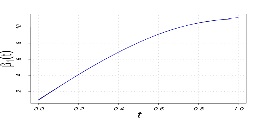
(a) $\beta_{1}(t)$

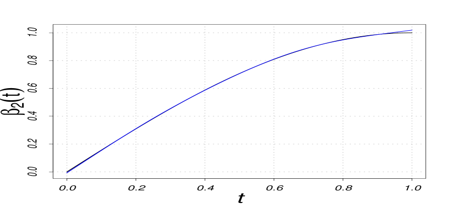
(b) $\beta_{2}(t)$

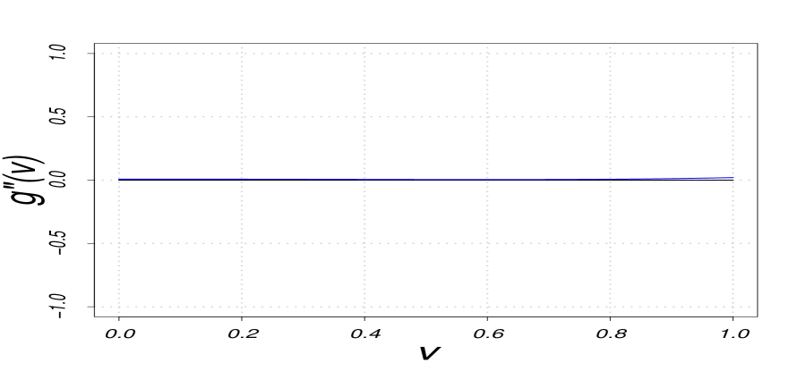
(c) $g^{\prime\prime}(v)$

Figure 1: The plots of $\beta_{1}(t)$, $\beta_{2}(t)$ and $g^{{}^{\prime\prime}}(v)$ for Example 1: $g(v)=10v+1$.

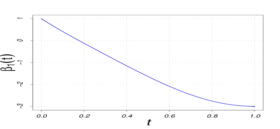
(a) $\beta_{1}(t)$

(b) $\beta_{2}(t)$

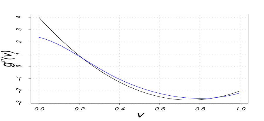
(c) $g^{\prime\prime}(v)$

Figure 2: The plots of $\beta_{1}(t)$, $\beta_{2}(t)$ and $g^{{}^{\prime\prime}}(v)$ for Example 2: $g(v)=1-4v+2v^{2}-3v^{3}+v^{4}$.

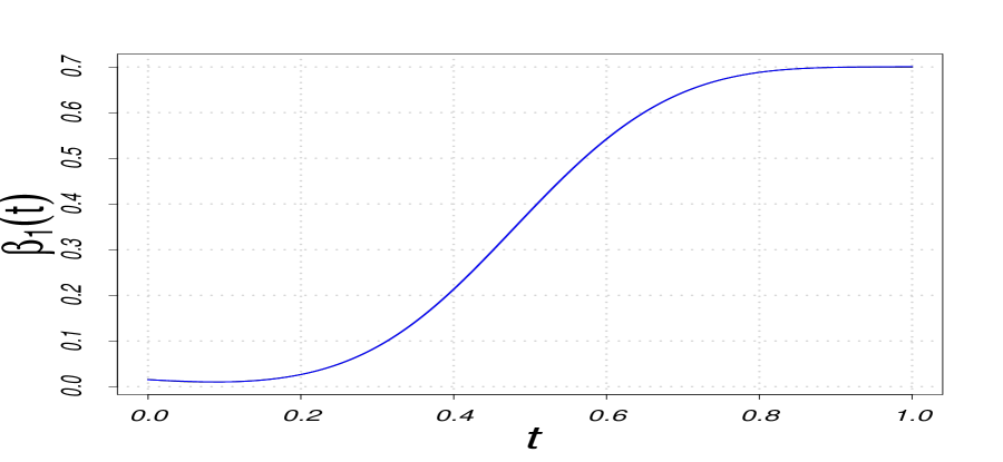
(a) $\beta_{1}(t)$

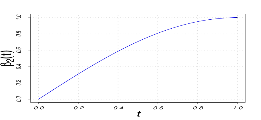
(b) $\beta_{2}(t)$

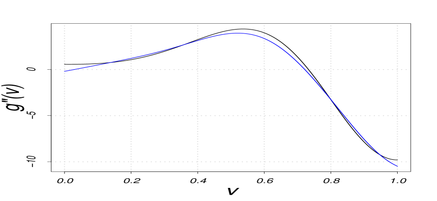
(c) $g^{\prime\prime}(v)$

Figure 3: The plots of $\beta_{1}(t)$, $\beta_{2}(t)$ and $g^{{}^{\prime\prime}}(v)$ for Example 3: $g(v)=0.3\exp(-3(v+1)^{2})+0.7\exp(-7(v-1)^{2})$.

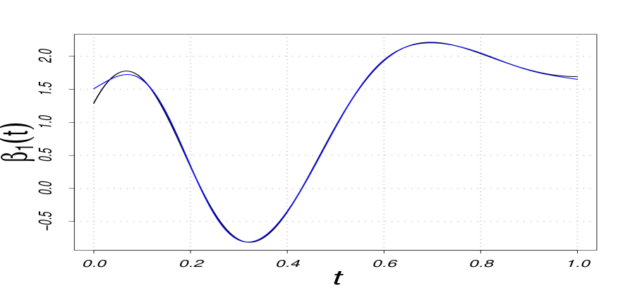
(a) $\beta_{1}(t)$

(b) $\beta_{2}(t)$

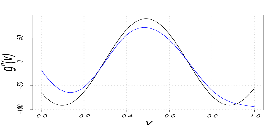
(c) $g^{\prime\prime}(v)$

Figure 4: The plots of $\beta_{1}(t)$, $\beta_{2}(t)$ and $g^{{}^{\prime\prime}}(v)$ for Example 4: $g(v)=\sin(8v)+\cos(8v)+\log(4/3+v)$.

(a) Density plot of $T_{n}$ for Example 1: $g(v)=10v+1$.

(b) Density plot of $T_{n}$ for Example 2: $g(v)=1-4v+2v^{2}-3v^{3}+v^{4}$

(c) Density plot of $T_{n}$ for Example 3: $g(v)=0.3\exp(-3(v+1)^{2})+0.7\exp(-7(v-1)^{2})$

(d) Density plot of $T_{n}$ for Example 4 $g(v)=\sin(8v)+\cos(8v)+\log(4/3+v)$

Figure 5: Density plots $T_{n}$ for different choices of $g$

6 Real data analysis

In this section, we illustrate the proposed methodology on DTI data set which is publicly available in refund (Goldsmith et al., 2020) package in R. The MRI/DTI data were collected at Johns Hopkins University and the Kennedy-Krieger Institute, where the clinical objective was to study the cerebral white-matter tracts of patients with multiple sclerosis (MS). It is an appropriate place to mention that MS is an autoimmune disease that causes lesions in the white matter tracts of affected individuals, leading to severe disability, and the DTI, i.e., diffusion tensor imaging tractography allows to study of the white matter tracts by measuring the diffusivity of the water in the brain (See Basser et al. (1994); Le Bihan et al. (2001) for more details). There are several measurements of water diffusion which include fractional anisotropy. This is a continuous summary of the white matter ($X$) tracts parameterized by the distance along the tracts ($t$) derived from DTI. There are 100 subjects with each subject having multiple visits. They undergo a collection of tests that assess cognitive and motor functions. Here we focus on the mean diffusivity profile of the corpus callosum tract as our functional covariates and the paced auditory serial addition test (PASAT), which is a common measure of cognitive function affected by MS with scores ranging between 0 and 60 as scalar outcome. We want to test whether there is a non-constant relationship of the functional covariates to predict PASAT for baseline and the immediate next visit. Figure 6 demonstrates the estimated coefficients and the estimated second derivative of the unknown function $g$. Using the proposed bootstrap methodology in Algorithm 1, we obtain the $p$-value as 0.571, which indicates that the data does favor the null hypothesis at $5\%$ level of significance. From the medical science point of view, one may conclude from this study that there is some linear functional relationship between the effect of functional covariates on scalar response PASAT score at two consecutive visits or the effect of functional covariates on scalar response PASAT score at the second visit does not depend on that of the first visit.

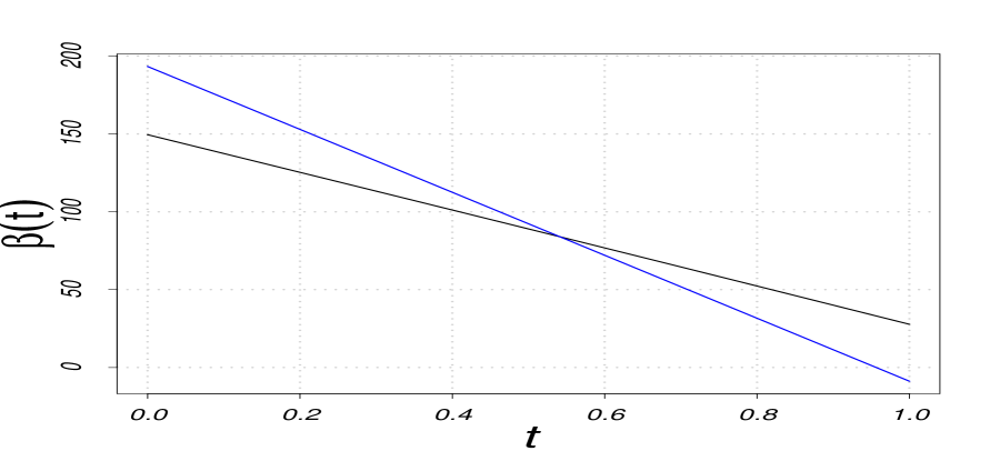
(a) $\beta_{1}(t)$ (black) and $\beta_{2}(t)$ (blue)

(b) $g^{\prime\prime}(v)$

Figure 6: The plots of $\beta_{1}(t)$, $\beta_{2}(t)$ and $g^{{}^{\prime\prime}}(v)$ based on the DTI analysis

7 Discussion

In this article, we tried to identify an unknown transformation between two slope functions associated with a scalar on a functional linear regression model for two independent data sets. To investigate it, we formulated a testing of the hypothesis problem and derived the asymptotic distribution of the test statistic. Moreover, wild bootstrap technique has also been adopted to implement the test for small sample sized data along with its theoretical justification. In this regard, we would like to emphasize that this work can be extended for the function on function linear regression as well. To avoid complexity of notations, the work is done for scalar on function regression.

The test and its methodology considered in this article can be extended for more than two independent samples. Here we are describing for the case of three samples for notational simplicity. Suppose that in (4), consider $s\in\{1,2,3\}$, and we want to test

$H_{0}:\beta_{1}(t)=g_{1}(\beta_{2}(t))$ for all linear transformation $g_{1}$ and $\beta_{3}(t)=g_{2}(\beta_{2}(t))$ for all linear transformation $g_{2}$.

against

$H_{1}:\beta_{1}(t)=g_{1}(\beta_{2}(t))$ for some non-linear transformation $g_{1}$ and $\beta_{3}(t)=g_{2}(\beta_{2}(t))$ for some non-linear transformation $g_{2}$.

Recall the test statistic $T_{n}$ from (22) in the case of two independent sample, where $n=\min(n_{1},n_{2})$. Now, similarly define the test statistic $T_{n^{*}}$ for the second and the third independent samples. Finally, in order to test the aforesaid null hypothesis described in $H_{0}$, one can propose the test statistic as

$$T_{n_{1},n_{2},n_{3}}=\min(T_{n},T_{n^{*}}).$$

In fact, in principle, one may extend this methodology for any finitely many independent samples. Similarly, one may modify the bootstrap algorithm 1 as well for the case of three independent samples or finitely many independent samples.

Code Availability: All codes for numerical studies and real data analysis are available to the first author upon request.

Acknowledgement: Subhra Sankar Dhar presented a part of this work at Renmin University of China when he was visiting there during summer, 2023, and many stimulating questions asked by the audience improved the content of the article. He is also thankful to Dr. Hengrui Cai of UC Irvine for a few interesting suggestions on various parts in this work. Finally, Subhra Sankar Dhar gratefully acknowledges his core research grant CRG/2022/001489, Government of India.

Appendix

For any sequence of random variables $\{Z_{n}\}_{n\geq 1}$, we denote $Z_{n}=O_{r}(a_{n})$ if $\mathbb{E}|Z_{n}|^{r}=O(a_{n}^{r})$. Therefore, it is straightforward to see that $Z_{n}=\mathbb{E}\{Z_{n}\}+O_{r}([\mathbb{E}\{Z_{n}-\mathbb{E}Z_{n}\}^{r}]^{1/r})$. Moreover, we define $Z_{n}=O_{\mathbb{P}}(a_{n})$ if for any positive $\epsilon$, $\mathbb{P}\{|Z_{n}|>\epsilon\}\rightarrow 0$ as $n\rightarrow\infty$. Due to Markov’s inequality, $O_{r}(a_{n})$ implies $O_{\mathbb{P}}(a_{n})$ for any sequence $a_{n}\rightarrow 0$ (see, e.g, Van Der Vaart et al. (1996)). Here we will state a few more lemma, which will be useful in proving the main results of this work.

Lemma 3.

For a sequence of random functions $\{X_{n}(t):t\in\mathcal{T}\}_{n\geq 1}$ defined on a compact support, if $\int_{\mathcal{T}}X^{2}(t)dt=O_{\mathbb{P}}(a_{n})$ then $\sup\limits_{t\in\mathcal{T}}|X(t)|=O_{\mathbb{P}}(a_{n}^{1/2})$.

Proof.

Without loss of generality, assume that $\mathcal{T}=[0,1]$. Then, observe that

$$\int X_{n}^{2}(t)dt\leq\{\sup|X_{n}(t)|\}^{2}.$$

Afterwards, note that, for any $\epsilon>0$ and $n\geq 1$, one has

$$\left\{\omega:\left(\int X_{n}^{2}(t,\omega)dt/a_{n}\right)^{1/2}>\epsilon\right\}\supseteq\left\{\omega:\sup|X_{n}(t,\omega)|>\epsilon\right\}.$$

Therefore, as $n\rightarrow\infty$, $\mathbb{P}\left\{\sup|X_{n}(t)|>\epsilon\right\}\leq\mathbb{P}\left\{\left(\int X_{n}^{2}(t)dt/a_{n}\right)^{1/2}>\epsilon\right\}\rightarrow 0$. ∎

Proof of Lemma 1.

Using the derivation of Theorem 1 in Hall et al. (2007) and Lemma 3, the result is immediate. ∎

Proof of Lemma 2.

Using the similar argument mentioned in Theorem 1 of Imaizumi and Kato (2018), the result is immediate. ∎

Before proving Theorems 4.1, 4.2, 4.3 and 4.4, recall $\mathbf{U}_{n_{1}}=(U_{1},\cdots,U_{m_{n_{1}}})^{\text{T}}$, $\mathbf{V}_{n_{2}}=(V_{1},\cdots,V_{m_{n_{2}}})^{\text{T}}$ where $U_{j}=\widehat{\beta}_{1}(t_{j})$, estimate of $\beta_{1}(t_{j})$ based on $n_{1}$ samples and $V_{j}=\widehat{\beta}_{2}(t_{j})$, estimate of $\beta_{2}(t_{j})$ based on $n_{2}$ samples for $j=1,\cdots,m$. Moreover, further recall $\eta_{j}=\widehat{\beta}_{1}(t_{j})-g(\widehat{\beta}_{2}(t_{j}))=U_{j}-g(V_{j})$, which depends on $n$ (see Section 3.2) is a random variable with mean zero and finite variance $\sigma_{n}^{2}$.

Proof of Theorem 4.1.

Observe that

$$g(V_{j})=g(v_{0})+g^{\prime}(v_{0})(V_{j}-v_{0})+\frac{1}{2}g^{\prime\prime}(v_{0})(V_{j}-v_{0})^{2}+R_{m_{n}}(v_{0},V_{j}),$$ (35)

where

$$R_{m_{n}}(v_{0},V_{j})=g(V_{j})-g^{\prime}(v_{0})(V_{j}-v_{0})-\frac{1}{2}g^{\prime\prime}(v_{0})(V_{j}-v_{0})^{2}.$$

Let us now denote $\mathbf{R}=(R(v_{0},V_{1}),\cdots.R(v_{0},V_{m_{n}}))^{\text{T}}$ and re-define

$$\mathcal{X}(v_{0}) =\begin{pmatrix}1&V_{1}-v_{0}&(V_{1}-v_{0})^{2}&(V_{1}-v_{0})^{3}\\ \vdots&\vdots&\vdots&\vdots\\ 1&V_{m_{n}}-v_{0}&(V_{m_{n}}-v_{0})^{2}&(V_{m_{n}}-v_{0})^{3}\end{pmatrix},$$

$$\mathcal{X}_{h_{m_{n}}}(v_{0}) =\begin{pmatrix}1&\frac{V_{1}-v_{0}}{h_{m_{n}}}&\frac{(V_{1}-v_{0})^{2}}{h_{m_{n}}^{2}}&\frac{(V_{1}-v_{0})^{3}}{h_{m_{n}}^{3}}\\ \vdots&\vdots&\vdots&\vdots\\ 1&\frac{V_{m_{n}}-v_{0}}{{m_{n}}}&\frac{V_{m_{n}}-v_{0})^{2}}{{m_{n}}^{2}}&\frac{(V_{m_{n}}-v_{0})^{3}}{{m_{n}}^{3}}\end{pmatrix},$$

$$\mbox{and}~{}~{}~{}~{}\Gamma_{h_{m_{n}}} =\begin{pmatrix}1&0&0&0\\ 0&h_{m_{n}}^{-1}&0&0\\ 0&0&h_{m_{n}}^{-2}&0\\ 0&0&0&h_{m_{n}}^{-3}\end{pmatrix}.$$

Thus, for a given point $v=v_{0}\in\mathbb{R}$, in the same spirit of (21), observe that

$$\widehat{g}_{h_{n}}^{\prime\prime}(v_{0})=\sum_{j=1}^{m}s_{j,h_{m_{n}}}(v_{0},2)\widehat{\beta}_{1}(t_{j})$$

$$=2\mathbf{e}_{3}^{\text{T}}\{\mathcal{X}(v_{0})^{\text{T}}\mathcal{W}_{h_{m_{n}}}(v_{0})\mathcal{X}(v_{0})\}^{-1}\{\mathcal{X}(v_{0})^{\text{T}}\mathcal{W}_{h_{m_{n}}}(v_{0})\mathbf{U}_{n_{1}}\}$$

$$=2\mathbf{e}_{3}^{\text{T}}\left\{\frac{1}{mh_{m_{n}}}\sum_{j=1}^{m_{n}}K\left(\frac{V_{j}-v_{0}}{h_{m_{n}}}\right)\left(1,\frac{V_{j}-v_{0}}{h_{m_{n}}},\frac{(V_{j}-v_{0})^{2}}{h_{m_{n}}^{2}},\frac{(V_{j}-v_{0})^{3}}{h_{n}^{3}}\right)^{\text{T}\otimes^{2}}\right\}^{-1}$$

$$\qquad\times\Bigg{\{}\frac{1}{m_{n}h_{m_{n}}}\sum_{j=1}^{m_{n}}K\left(\frac{V_{j}-v_{0}}{h_{m_{n}}}\right)\left(1,\frac{V_{j}-v_{0}}{h_{m_{n}}},\frac{(V_{j}-v_{0})^{2}}{h_{m_{n}}^{2}},\frac{(V_{j}-v_{0})^{3}}{h_{m_{n}}^{3}}\right)^{\text{T}}\Bigg{.}$$

$$\qquad\qquad\Bigg{.}\times\left[g(v_{0})+g^{\prime}(v_{0})(V_{j}-v_{0})+\frac{1}{2}g^{\prime\prime}(v_{0})(V_{j}-v_{0})^{2}+R_{m}(v_{0},V_{j})+\eta_{j}\right]\Bigg{\}}$$

$$=g^{\prime\prime}(v_{0})+2\mathbf{e}_{3}^{\text{T}}\left\{\frac{1}{mh_{m_{n}}}\sum_{j=1}^{m_{n}}K\left(\frac{V_{j}-v_{0}}{h_{m_{n}}}\right)\left(1,\frac{V_{j}-v_{0}}{h_{m_{n}}},\frac{(V_{j}-v_{0})^{2}}{h_{m_{n}}^{2}},\frac{(V_{j}-v_{0})^{3}}{h_{m_{n}}^{3}}\right)^{\text{T}\otimes^{2}}\right\}^{-1}$$

$$\qquad\times\left\{\frac{1}{mh_{n}}\sum_{j=1}^{m_{n}}K\left(\frac{V_{j}-v_{0}}{h_{m_{n}}}\right)\left(1,\frac{V_{j}-v_{0}}{h_{m_{n}}},\frac{(V_{j}-v_{0})^{2}}{h_{m_{n}}^{2}},\frac{(V_{j}-v_{0})^{3}}{h_{m_{n}}^{3}}\right)^{\text{T}}\left[R_{m_{n}}(v_{0},V_{j})+\eta_{j}\right]\right\}$$

$$:=g^{\prime\prime}(v_{0})+2\mathbf{e}_{3}^{\text{T}}\mathbf{A}_{1}^{-1}(v_{0})\left\{\mathbf{A}_{2}(v_{0})+\mathbf{A}_{3}(v_{0})\right\},$$ (36)

where

$$\mathbf{A}_{1}(v_{0}) =\frac{1}{m_{n}h_{m_{n}}}\sum_{j=1}^{m_{n}}K\left(\frac{V_{j}-v_{0}}{h_{m_{n}}}\right)\left(1,\frac{(V_{j}-v_{0})}{h_{m_{n}}},\frac{(V_{j}-v_{0})^{2}}{h_{m_{n}}^{2}},\frac{(V_{j}-v_{0})^{3}}{h_{m_{n}}^{3}}\right)^{\text{T}\otimes^{2}},$$

$$\mathbf{A}_{2}(v_{0}) =\frac{1}{m_{n}h_{m_{n}}}\sum_{j=1}^{m_{n}}R_{m_{n}}(v_{0},V_{j})K\left(\frac{V_{j}-v_{0}}{h_{m_{n}}}\right)\left(1,\frac{(V_{j}-v_{0})}{h_{m_{n}}},\frac{(V_{j}-v_{0})^{2}}{h_{m_{n}}^{2}},\frac{(V_{j}-v_{0})^{3}}{h_{m_{n}}^{3}}\right)^{\text{T}},$$

$$\mbox{and}~{}\mathbf{A}_{3}(v_{0}) =\frac{1}{m_{n}h_{m_{n}}}\sum_{j=1}^{m}\eta_{j}K\left(\frac{V_{j}-v_{0}}{h_{m_{n}}}\right)\left(1,\frac{(V_{j}-v_{0})}{h_{m_{n}}},\frac{(V_{j}-v_{0})^{2}}{h_{m_{n}}^{2}},\frac{(V_{j}-v_{0})^{3}}{h_{m_{n}}^{3}}\right)^{\text{T}}.$$

Now, under condition (K1) and in view of the assertion in Lemma 2, using Taylor’s series expansion, for any integer $c\in\{0,\cdots,6\}$, we have

$$\mathbb{E}\left\{\frac{1}{m_{n}h_{m_{n}}}\sum_{j=1}^{m_{n}}\left(\frac{V_{j}-v_{0}}{h_{m_{n}}}\right)^{c}K\left(\frac{V_{j}-v_{0}}{h_{m_{n}}}\right)\right\}$$

$$=\int K_{h_{m_{n}}}(v-v_{0})\left(\frac{v-s_{0}}{h_{m_{n}}}\right)^{c}f_{\widehat{\beta}_{2}}(v)dv$$

$$=\int v^{c}K(v)f_{\widehat{\beta}_{2}}(v_{0}+h_{m_{n}}v)dv$$

$$=\int v^{c}K(v)\left\{f_{\widehat{\beta}_{2}}(v_{0})+h_{m_{n}}vf_{\widehat{\beta}_{2}}^{[1]}(v_{0})+\frac{1}{2}h_{m_{n}}^{2}v^{2}f_{\widehat{\beta}_{2}}^{[2]}(v_{0}^{*})\right\}dv,\mbox{ where~{}$v_{0}^{*}\in(v,v_{0})$}$$

$$=\begin{cases}O\left(h_{m_{n}}f_{\widehat{\beta}_{2}}^{[1]}(v_{0})\right),&\text{for odd $c$ with $\nu_{c+1,1}<\infty$}\\ &\text{and $f_{\widehat{\beta}_{2}}^{[1]}(v_{0})<\infty$}\\ \nu_{c,1}f_{\widehat{\beta}_{2}}(v_{0})+O\left(h_{m_{n}}f_{\widehat{\beta}_{2}}^{[2]}(v_{0})\right),&\text{for even $c$ is with $\nu_{c+1,1}<\infty$}\\ &\text{and $f_{\widehat{\beta}_{2}}^{[2]}(v_{0})<\infty$}.\\ \end{cases}$$ (37)

Here $v_{0}$ is an arbitrary point $v_{0}$ in the support of $f_{\widehat{\beta}_{s}}(.)$, where $f_{\widehat{\beta}_{s}}^{[j]}(.)$ denotes the $j$-th derivatives of $f_{\widehat{\beta}_{s}}(.)$.

Next, arguing in a similar way, one can derive

$$\mathbb{E}\left\{\frac{1}{m_{n}^{2}h_{m_{n}}^{2}}\sum_{j=1}^{m_{n}}\left(\frac{V_{j}-v_{0}}{h_{m_{n}}}\right)^{c}K^{2}\left(\frac{V_{j}-v_{0}}{h_{m_{n}}}\right)\right\}$$

$$=\frac{1}{m_{n}h_{m_{n}}^{2}}\mathbb{E}\left\{\left(\frac{V-v_{0}}{h_{m_{n}}}\right)^{c}K^{2}\left(\frac{V-v_{0}}{h_{m_{n}}}\right)\right\}$$

$$=\frac{1}{m_{n}h_{m_{n}}}\int K^{2}_{h_{n}}(v-v_{0})\left(\frac{v-v_{0}}{h_{m_{n}}}\right)^{c}f_{\widehat{\beta}_{2}}(v)dv$$

$$=\frac{1}{m_{n}h_{m_{n}}}\int v^{c}K^{2}(v)\left\{f_{\widehat{\beta}_{2}}(v_{0})+h_{m_{n}}vf_{\widehat{\beta}_{2}}^{[1]}(v_{0})+0.5h_{m_{n}}^{2}v^{2}f_{\widehat{\beta}_{2}}^{[2]}(v_{0}^{**})\right\}dv,~{}\mbox{where $v_{0}^{**}\in(v,v_{0})$}$$

$$=\frac{1}{m_{n}h_{m_{n}}}\begin{cases}O\left(h_{m_{n}}f_{\widehat{\beta}_{2}}^{[1]}(v_{0})\right),&\text{for odd $c$ with $\nu_{c+1,2}<\infty$}\\ &\text{and $f_{\widehat{\beta}_{2}}^{[1]}(v_{0})<\infty$}\\ \nu_{c,2}f_{\widehat{\beta}_{2}}(v_{0})+O\left(h_{m_{n}}^{2}f_{\widehat{\beta}_{2}}^{[2]}(v_{0})\right),&\text{for even $c$ with $\nu_{c+1,2}<\infty$}\\ &\text{and $f_{\widehat{\beta}_{2}}^{[2]}(v_{0})<\infty$}\\ \end{cases}.$$ (38)

Therefore, for $c\in\{0,\cdots,6\}$, using condition (K1) and Lemma 2, we have

$$\text{Var}\left\{\frac{1}{m_{n}h_{m_{n}}}\sum_{j=1}^{m_{n}}\left(\frac{V_{j}-v_{0}}{h_{m_{n}}}\right)^{c}K\left(\frac{V_{j}-v_{0}}{h_{m_{n}}}\right)\right\}$$

$$\lesssim\mathbb{E}\left\{\frac{1}{m_{n}^{2}h_{m_{n}}^{2}}\sum_{j=1}^{m_{n}}\left(\frac{V_{j}-v_{0}}{h_{m_{n}}}\right)^{2c}K^{2}\left(\frac{V_{j}-v_{0}}{h_{m_{n}}}\right)\right\}=O\left(\frac{f_{\widehat{\beta}_{2}}(v_{0})}{m_{n}h_{m_{n}}}\right).$$ (39)

Besides, Lemma 2 asserts that, conditioning on $V_{1},\cdots,V_{m_{n}}$,

$$\mathbf{A}_{1}(v_{0})=f_{\widehat{\beta}_{2}}(v_{0})\underbrace{\begin{pmatrix}1&0&\nu_{2,1}&0\\ 0&\nu_{2,1}&0&\nu_{4,1}\\ \nu_{2,1}&0&\nu_{4,1}&0\\ 0&\nu_{4,1}&0&\nu_{6,1}\end{pmatrix}}_{:=\boldsymbol{\Omega}}+O\left(h_{m_{n}}f_{\widehat{\beta}_{2}}^{[1]}(v_{0})\right)+O_{2}\left(\sqrt{\frac{f_{\widehat{\beta}_{2}}(v_{0})}{m_{n}h_{m_{n}}}}\right).$$ (40)

and a few steps of straightforward algebra gives us

$$\mathbf{e}_{3}^{\text{T}}\mathbf{A}_{1}^{-1}(v_{0})=\frac{1}{f_{\widehat{\beta}_{2}}(v_{0})}(a_{1},0,a_{2},0)^{\text{T}}+O\left(h_{m_{n}}f_{\widehat{\beta}_{2}}^{[1]}(v_{0})\right)+O_{2}\left(\sqrt{\frac{f_{\widehat{\beta}_{2}}(v_{0})}{m_{n}h_{m_{n}}}}\right),$$ (41)

where

$$a_{1}=\frac{\nu_{2,1}\nu_{4,1}^{2}-\nu_{2,1}^{2}\nu_{6,1}}{\nu_{2,1}^{2}\nu_{4,1}^{2}-\nu_{4,1}^{2}-\nu_{2,1}^{3}\nu_{6,1}+\nu_{2,1}\nu_{4,1}\nu_{6,1}},$$

and

$$a_{2}=\frac{-\nu_{4,1}^{2}+\nu_{2,1}\nu_{6,1}}{\nu_{2,1}^{2}\nu_{4,1}^{2}-\nu_{4,1}^{3}-\nu_{2,1}^{3}\nu_{6,1}+\nu_{2,1}\nu_{4,1}\nu_{6,1}}.$$

Afterwards, for $c\in\{0,1,2,3\}$ conditioning on $V_{1},\cdots,V_{m_{n}}$, we obtain,

$$\frac{1}{m_{n}h_{m_{n}}}\sum_{j=1}^{m_{n}}R_{m_{n}}(v_{0},V_{j})\left(\frac{V_{j}-v_{0}}{h_{m_{n}}}\right)^{c}K\left(\frac{V_{j}-v_{0}}{h_{m_{n}}}\right)$$

$$=\frac{1}{h_{m_{n}}}\int R_{m_{n}}(v_{0},v)\left(\frac{v-v_{0}}{h_{m_{n}}}\right)^{c}K\left(\frac{v-v_{0}}{h_{m_{n}}}\right)f_{\widehat{\beta}_{2}}(v)dv+O_{2}\left(\sqrt{\frac{f_{\widehat{\beta}_{2}}(v_{0})}{m_{n}h_{m_{n}}}}\right)$$

$$=\int R_{m_{n}}(v_{0},v_{0}+h_{m_{n}}v)v^{c}K(v)f_{\widehat{\beta}_{2}}(v_{0}+h_{m_{n}}v)dv+O_{2}\left(\sqrt{\frac{f_{\widehat{\beta}_{2}}(v_{0})}{m_{n}h_{m_{n}}}}\right)$$

$$\overset{(i)}{=}\int\frac{1}{2}\left(g^{\prime\prime}(v_{\star})-g^{\prime\prime}(v_{0})\right)v^{2+c}K(u)f_{\widehat{\beta}_{2}}(v_{0}+h_{m_{n}}v)dv+O_{2}\left(\sqrt{\frac{f_{\widehat{\beta}_{2}}(v_{0})}{m_{n}h_{m_{n}}}}\right)$$

$$=O\left(f_{\widehat{\beta}_{2}}(v_{0})h_{m_{n}}^{\delta+2}\right)+O_{2}\left(\sqrt{\frac{f_{\widehat{\beta}_{2}}(v_{0})}{m_{n}h_{m_{n}}}}\right).$$ (42)

The equality holds in $(i)$ due to mean value theorem, where $|v_{\star}-v_{0}|\leq h_{m_{n}}v$. Hence, by condition (K1) and Lemma 2, we have

$$\mathbb{E}\left\{\widehat{g}_{h_{n}}^{\prime\prime}(v_{0})\right\}-g^{\prime\prime}(v_{0})$$

$$=\mathbb{E}\left\{2\mathbf{e}_{3}^{\text{T}}\left[\frac{\mathbf{A}_{1}^{-1}(v_{0})}{f_{\widehat{\beta}_{2}}(v_{0})}+O(h_{n})+O_{2}(1/\sqrt{mh_{n}})\right]\mathbf{A}_{2}(v_{0})\right\}$$

$$O\left(\left\{\frac{1}{f_{\widehat{\beta}_{2}(v_{0})}}+h_{m_{n}}f_{\widehat{\beta}_{2}}^{[1]}(v_{0})+\sqrt{\frac{f_{\widehat{\beta}_{2}}(v_{0})}{mh_{m_{n}}}}\right\}\left\{f_{\widehat{\beta}_{2}}(v_{0})h_{m_{n}}^{\delta+2}+\sqrt{\frac{f_{\widehat{\beta}_{2}}(v_{0})}{mh_{m_{n}}}}\right\}\right).$$ (43)

Next, we consider

$$\mathbb{E}\left\{\mathcal{X}^{\text{T}}(v_{0})\mathcal{W}_{h_{m_{n}}}^{2}(v_{0})\mathcal{X}(v_{0})\right\}$$

$$=\frac{1}{m_{n}^{2}h_{m_{n}}^{2}}\mathbb{E}\left\{\sum_{j=1}^{m_{n}}K^{2}_{h_{m_{n}}}\left(\frac{V_{j}-v_{0}}{h_{m_{n}}}\right)\left(1,\frac{V_{j}-v_{0}}{h_{m_{n}}},\frac{(V_{j}-v_{0})^{2}}{h_{m_{n}}^{2}},\frac{(V_{j}-v_{0})^{3}}{h_{m_{n}}^{3}}\right)^{\text{T}\otimes^{2}}\right\}$$

$$=\frac{1}{m_{n}h_{m_{n}}}\left\{f_{\widehat{\beta}_{2}}(v_{0})\begin{pmatrix}\nu_{2,0}&0&\nu_{2,2}&0\\ 0&\nu_{2,2}&0&\nu_{4,2}\\ \nu_{2,2}&0&\nu_{4,2}&0\\ 0&\nu_{4,2}&0&\nu_{6,2}\end{pmatrix}+O\left(h_{m_{n}}f_{\widehat{\beta}_{2}}(v_{0})\right)\right\}.$$ (44)

The last equality in the above expression holds due to the similar derivation of the expression (Proof of Theorem 4.1.). Hence, we have the following using condition ((E2)).

$$\text{Var}\left\{\widehat{g}_{h_{m_{n}}}^{\prime\prime}(v_{0})\right\}$$

$$\leq 4\mathbb{E}\left\{\mathbf{e}_{3}^{\text{T}}\mathbf{A}_{1}^{-1}(v_{0})\mathcal{X}^{\text{T}}(v_{0})\mathcal{W}_{h_{m_{n}}}(v_{0})\mathbf{U}_{n_{1}}\mathbf{U}_{n_{1}}^{\text{T}}\mathcal{W}_{h_{m_{n}}}(v_{0})\mathcal{X}(v_{0})\mathbf{A}_{1}^{-1}(v_{0})\mathbf{e}_{3}\right\}$$

$$\lesssim\sigma_{n}^{2}\mathbf{e}_{3}^{\text{T}}\mathbf{A}_{1}(v_{0})^{-1}\mathbb{E}\left\{\mathcal{X}_{h_{m_{n}}}(v_{0})^{\text{T}}\mathcal{W}_{h_{m_{n}}}(v_{0})\mathcal{W}_{h_{m_{n}}}(v_{0})\mathcal{X}_{h_{m_{n}}}(v_{0})\right\}\mathbf{A}_{1}(v_{0})^{-1}\mathbf{e}_{3}$$

$$=O\left(\frac{\sigma^{2}_{n}}{m_{n}h_{m_{n}}^{5}f_{\widehat{\beta}_{2}}(v_{0}))}\right).$$ (45)

The proof is complete. ∎

Lemma 4.

Let $\{Z_{n}(v)\}_{n\geq 1}$ be a sequence of random functions defined on $[v_{1},v_{2}]\subset\mathbb{R}$, such that $\sup\limits_{v\in[v_{1},v_{2}]}|Z_{n}(v)|=O_{\mathbb{P}}(a_{n})$, where $\{a_{n}\}_{n\geq 1}$ is a sequence of positive real numbers with $\displaystyle\lim_{n\rightarrow\infty}a_{n}=0$. Suppose that for any $\delta>0$, there exits $M(\delta)>0$ such that $\mathbb{P}[\widehat{v}_{1}<v_{1}-M]<\delta$ and $\mathbb{P}[\widehat{v}_{2}>v_{2}+M]<\delta$. Then, $\sup\limits_{v\in[\widehat{v}_{1},\widehat{v}_{2}]}|Z_{n}(v)|=O_{\mathbb{P}}(a_{n})$.

Proof.

As for a fixed $v$, $Z_{n}(v)$ is a sequence of random variables, for any $\epsilon>0$, there exits a constant $C(\epsilon)>0$ and $N(\epsilon)\in\mathbb{N}$ such that for all $n\geq N$,

$$\mathbb{P}\left\{\sup_{v\in[v_{1},v_{2}]}|Z_{n}(v)|>Ca_{n}\right\}<\epsilon.$$ (46)

Further, observe that

$$\mathbb{P}\{\widehat{v}_{1}\in[v_{1}-M,v_{2}+M]\cap\widehat{v}_{2}\in[v_{1}-M,v_{2}+M]\}\geq(1-2\delta)$$

in view of the assertions on $\widehat{v}_{l}$ and $v_{l}$ stated in the statement of this lemma, where $l\in\{1,2\}$. In addition, we also have

$$\sup_{v\in[\widehat{v}_{1},\widehat{v}_{2}]}|Z_{n}(v)|\leq\sup_{v\in[{v}_{1}-M,{v}_{2}+M]}|Z_{n}(v)|$$ (47)

In addition, by the assumption of $\sup\limits_{v\in[v_{1}-M,v_{2}+M]}|Z_{n}(v)|=O_{\mathbb{P}}(a_{n})$, we can write for baby $\epsilon>0$, there exists a generic constant $C>0$ and $N(\epsilon)\in\mathbb{N}$ such that for $n\geq N$,

$$\mathbb{P}\left\{\sup_{v\in[{v}_{1}-M,{v}_{2}+M]}|Z_{n}(v)|>Ca_{n}\right\}>\epsilon-2\delta.$$ (48)

Hence, by combining inequalities in (47) and (48),

$$\mathbb{P}\left\{\sup\limits_{v\in[\widehat{v}_{1},\widehat{v}_{2}]}|Z_{n}(v)|>Ca_{n}\right\}$$

$$\leq\mathbb{P}\left\{\sup_{v\in[{v}_{1}-M,{v}_{2}+M]}|Z_{n}(v)|>Ca_{n}\right\}+\mathbb{P}\left\{\widehat{v}_{1}\notin[v_{1}-M,v_{2}+M]\cup\widehat{v}_{2}\notin[v_{1}-M,v_{2}+M]\right\}$$

$$<(\epsilon-2\delta)+2\delta=\epsilon.$$ (49)

This completes the proof. ∎

Proof of Theorem 4.2.

First, we need to need to show that, under (K1), (K2), (G1) (B1) and the assertion in Lemma 2, for some real constants $v_{1}<v_{2}$, the scaled difference $d_{h_{m_{n}}}(v):=\sqrt{m_{n}h_{m_{n}}^{5}}\left(\widehat{g}_{h_{m_{n}}}^{\prime\prime}(v)-\mathbb{E}\left\{\widehat{g}_{h_{m_{n}}}^{\prime\prime}(v)\right\}\right)$ has the following approximation:

$$\sup_{v\in[v_{1},v_{2}]}\left|\frac{d_{m_{n}}-\frac{1}{\sqrt{h_{m_{n}}}}\mathbb{G}_{m_{n}}[\mathbf{e}^{\text{T}}\boldsymbol{\Omega}^{-1}\boldsymbol{\Psi}_{m_{n}}(v)]}{\frac{1}{\sqrt{h_{m_{n}}}}\mathbb{G}_{m_{n}}[\mathbf{e}_{3}^{\text{T}}\boldsymbol{\Psi}_{h_{m_{n}}}(v)]}\right|=O(h_{m_{n}})+O_{\mathbb{P}}\left(\sqrt{\frac{\log m_{n}}{m_{n}h_{m_{n}}}}\right),$$ (50)

where $\mathbb{G}_{m_{n}}$, $\boldsymbol{\Omega}$ and $\boldsymbol{\Psi}_{m_{n}}$ are defined in Section 4.

In order to establish (50), note that the scaled difference can be expressed as

$$d_{h_{m_{n}}}(v) =\sqrt{m_{n}h_{m_{n}}^{5}}\left(\widehat{g}_{h_{m_{n}}}^{\prime\prime}(v)-\mathbb{E}\left\{\widehat{g}_{h_{m_{n}}}^{\prime\prime}(v)\right\}\right)$$

$$=\sqrt{m_{n}h_{m_{n}}^{5}}\left(\widehat{g}_{h_{m_{n}}}^{\prime\prime}(v)-g^{\prime\prime}(v)\right)+\sqrt{m_{n}h_{m_{n}}^{5}}\left(g^{\prime\prime}(v)-\mathbb{E}\left\{\widehat{g}_{h_{m_{n}}}^{\prime\prime}(v)\right\}\right).$$ (51)

Using the fact in Theorem 4.1, observe that

$$\sqrt{m_{n}h_{m_{n}}^{5}}\left(g^{\prime\prime}(v)-\mathbb{E}\left\{\widehat{g}_{h_{m_{n}}}^{\prime\prime}(v)\right\}\right)=o_{p}(1)$$

as $m_{n}h_{m_{n}}^{1/5}\rightarrow c$, for some constant $c$. Therefore, one can conclude that

$$d_{h_{m_{n}}}(v)=\sqrt{m_{n}h_{m_{n}}^{5}}\left(\widehat{g}_{h_{m_{n}}}^{\prime\prime}(v)-g^{\prime\prime}(v)\right)+o_{\mathbb{P}}(1).$$

Now, one can simplify the expression of $\widehat{g}_{h_{m_{n}}}^{\prime\prime}(v)$ as follow.

$$\widehat{g}_{h_{m_{n}}}^{\prime\prime}(v)=2\mathbf{e}_{3}^{\text{T}}\left\{\mathcal{X}^{\text{T}}(v)\mathcal{W}_{h_{m_{n}}}(v)\mathcal{X}(v)\right\}^{-1}\mathcal{X}^{\text{T}}(v)\mathcal{W}_{h_{m_{n}}}\mathbf{U}_{n_{1}}$$

$$=\frac{2\mathbf{e}_{3}^{\text{T}}\Gamma_{h_{m_{n}}}}{h_{m_{n}}^{2}}\left\{\frac{1}{m_{n}h_{n}}\Gamma_{h_{m_{n}}}\mathcal{X}^{\text{T}}(v)\mathcal{W}_{h_{m_{n}}}(v)\mathcal{X}(v)\Gamma_{h_{m_{n}}}\right\}^{-1}\frac{1}{h_{m_{n}}}\Gamma_{h_{m_{n}}}\mathcal{X}^{\text{T}}(v)\mathcal{W}_{h_{m_{n}}}\mathbf{U}_{n_{1}}$$

$$=\frac{2\mathbf{e}_{3}^{\text{T}}}{h_{m_{n}}^{2}}\left\{\frac{1}{m_{n}h_{m_{n}}}\mathcal{X}_{h_{m_{n}}}^{\text{T}}(v)\mathcal{W}_{h_{m_{n}}}(v)\mathcal{X}_{h_{m_{n}}}(v)\right\}^{-1}\frac{1}{m_{n}h_{m_{n}}}\mathcal{X}_{h_{m_{n}}}^{-1}(v)\mathcal{W}_{h_{m_{n}}}(v)\mathbf{U}_{n_{1}}$$

$$=\frac{2\mathbf{e}_{3}^{\text{T}}}{h_{m_{n}}^{2}}\left(\frac{\boldsymbol{\Omega}^{-1}}{f_{\widehat{\beta}_{2}}(v)}+O(h_{m_{n}})+O_{\mathbb{P}}\left(\sqrt{\frac{\log m_{n}}{m_{n}h_{m_{n}}}}\right)\right)\frac{1}{m_{n}h_{m_{n}}}\mathcal{X}_{h_{m_{n}}}^{\text{T}}(v)\mathcal{W}_{h_{m_{n}}}(v)\mathbf{U}_{n_{1}},$$ (52)

where $\mathbf{U}_{n_{1}}=(U_{1},\cdots,U_{m_{n_{1}}})^{\text{T}}$.

Further, we also have

$$\frac{1}{m_{n}h_{m_{n}}}\mathcal{X}_{h_{m_{n}}}^{\text{T}}(v)\mathcal{W}_{h_{m_{n}}}(v)\mathbf{U}_{n_{1}} =\begin{pmatrix}\frac{1}{m_{n}h_{m_{n}}}\sum\limits_{i=1}^{m_{n}}U_{i}K\left(\frac{V_{i}-v}{h_{m_{n}}}\right)\\ \frac{1}{m_{n}h_{m_{n}}}\sum\limits_{i=1}^{m_{n}}U_{i}\left(\frac{V_{i}-v}{h_{m_{n}}}\right)K\left(\frac{V_{i}-v}{h_{m_{n}}}\right)\\ \frac{1}{m_{n}h_{m_{n}}}\sum\limits_{i=1}^{m_{n}}U_{i}\left(\frac{V_{i}-v}{h_{m_{n}}}\right)^{2}K\left(\frac{V_{i}-v}{h_{m_{n}}}\right)\\ \frac{1}{m_{n}h_{m_{n}}}\sum\limits_{i=1}^{m_{n}}U_{i}\left(\frac{V_{i}-v}{h_{m_{n}}}\right)^{3}K\left(\frac{V_{i}-v}{h_{m_{n}}}\right)\end{pmatrix}$$

$$=\frac{1}{h_{m_{n}}}\int\boldsymbol{\Psi}(v;Z_{1},Z_{2})d\mathbb{P}_{m_{n}}(Z_{1},Z_{2}),$$ (53)

where

$$\boldsymbol{\Psi}_{h_{m_{n}}}(v;z_{1},z_{2})=(\psi_{0,h_{m_{n}}}(v;z_{1},z_{2}),\psi_{1,h_{m_{n}}}(v;z_{1},z_{2}),\psi_{2,h_{m_{n}}}(v;z_{1},z_{2}),\psi_{3,h_{m_{n}}}(v;z_{1},z_{2}))^{\text{T}}$$

as defined in Section 4. Each element of the vector $\boldsymbol{\Psi}_{h_{m_{n}}}$ is defined as

$$\psi_{c,h_{m_{n}}}(v,z_{1},z_{2})=z_{2}\left(\frac{z_{1}-v}{h_{m_{n}}}\right)^{c}K\left(\frac{z_{1}-v}{h_{m_{n}}}\right)$$

for $c\in\{0,1,2,3\}$. Therefore, using (Proof of Theorem 4.2.), one has

$$\widehat{g}_{h_{m_{n}}}^{\prime\prime}(v) =\frac{2}{h_{m_{n}}^{3}}\int\frac{\mathbf{e}_{3}^{\text{T}}\boldsymbol{\Omega}^{-1}\boldsymbol{\Psi}(v,Z_{1},Z_{2})}{f_{\widehat{\beta}_{2}}(v)}d\mathbb{P}_{m_{n}}(Z_{1},Z_{2})$$

$$\qquad+\frac{2}{h_{m_{n}}^{3}}\int\mathbf{e}_{3}^{\text{T}}\boldsymbol{\Psi}_{h_{m_{n}}}(v)(v;Z_{1},Z_{2})d\mathbb{P}_{m_{n}}(Z_{1},Z_{2})\left\{O\left(h_{m_{n}}\right)+O_{\mathbb{P}}\left(\sqrt{\frac{\log m_{n}}{m_{n}h_{m_{n}}}}\right)\right\}$$

$$=\frac{1}{h_{m_{n}}^{3}}\mathbb{P}_{m}[\mathbf{e}_{3}^{\text{T}}\mathbf{A}_{1}^{-1}\boldsymbol{\Psi}_{h_{m_{n}}}(v)]$$

$$\qquad+\frac{1}{h_{m_{n}}^{3}}\mathbb{P}_{m_{n}}[\mathbf{e}_{3}^{\text{T}}\boldsymbol{\Psi}_{h_{m_{n}}}(v)]\left\{O\left(h_{m_{n}}\right)+O_{\mathbb{P}}\left(\sqrt{\frac{\log m_{n}}{m_{n}h_{m_{n}}}}\right)\right\},$$ (54)

where

$$\mathbb{P}_{m_{n}}[\mathbf{e}_{3}^{\text{T}}\boldsymbol{\Omega}^{-1}\boldsymbol{\Psi}_{h_{m_{n}}}(v)]=\int 2\mathbf{e}_{3}^{\text{T}}\boldsymbol{\Omega}^{-1}\boldsymbol{\Psi}_{h_{m_{n}}}(v;Z_{1},Z_{2})d\mathbb{P}_{m_{n}}(Z_{1},Z_{2})$$

and

$$\mathbb{P}_{m_{n}}[\mathbf{e}_{3}^{\text{T}}\boldsymbol{\Psi}_{h_{m_{n}}}(v)]=\int 2\mathbf{e}_{3}^{\text{T}}\boldsymbol{\Psi}_{h_{m_{n}}}(v;Z_{1},Z_{2})d\mathbb{P}_{m_{n}}(Z_{1},Z_{2}).$$

Hence, we have

$$\mathbb{E}\left\{\widehat{g}_{h_{m_{n}}}^{\prime\prime}(v)\right\}=\frac{1}{h_{m_{n}}^{3}}\mathbb{P}[\mathbf{e}_{3}^{\text{T}}\boldsymbol{\Omega}\boldsymbol{\Psi}_{h_{m_{n}}}(v)]+\frac{1}{h_{m_{n}}^{3}}\mathbb{P}[\mathbf{e}_{3}^{\text{T}}\boldsymbol{\Psi}_{h_{m_{n}}}(v)]\left\{O\left(h_{m_{n}}\right)+O\left(\sqrt{\frac{\log m_{n}}{m_{n}h_{m_{n}}}}\right)\right\},$$ (55)

where

$$\mathbb{P}[\mathbf{e}_{3}^{\text{T}}\boldsymbol{\Omega}^{-1}\boldsymbol{\Psi}_{h_{m_{n}}}(v)]=\mathbb{E}\left\{\mathbb{P}_{m_{n}}[\mathbf{e}_{3}^{\text{T}}\mathbf{A}_{1}^{-1}\boldsymbol{\Psi}_{h_{m_{n}}}(v)]\right\}$$

and

$$\mathbb{P}[\mathbf{e}_{3}^{\text{T}}\boldsymbol{\Psi}_{h_{m_{n}}}(v)]=\mathbb{E}\left\{\mathbb{P}_{m_{n}}[\mathbf{e}_{3}^{\text{T}}\boldsymbol{\Psi}_{h_{m_{n}}}(v)]\right\}.$$

Summarizing the facts in (Proof of Theorem 4.2.) and (55), we have

$$d_{m_{n}}(v)=\sqrt{m_{n}h_{m_{n}}^{5}}\left(\widehat{g}_{h_{m_{n}}}^{\prime\prime}(v)-\mathbb{E}\left\{\widehat{g}^{\prime\prime}_{h_{m_{n}}}(v)\right\}\right)$$

$$=\sqrt{\frac{{m_{n}}}{h_{m_{n}}}}\left(\mathbb{P}_{m_{n}}-\mathbb{P}\right)[\mathbf{e}^{\text{T}}\boldsymbol{\Omega}^{-1}\boldsymbol{\Psi}_{h_{m_{n}}}(v)]$$

$$\qquad+\sqrt{\frac{{m_{n}}}{h_{m_{n}}}}\left(\mathbb{P}_{m_{n}}-\mathbb{P}\right)[\mathbf{e}_{3}^{\text{T}}\boldsymbol{\Psi}_{h_{m_{n}}}(v)]\left\{O\left(h_{m_{n}}\right)+O_{\mathbb{P}}\left(\sqrt{\frac{\log m_{n}}{m_{n}h_{m_{n}}}}\right)\right\}$$

$$=\frac{1}{\sqrt{h_{m_{n}}}}\mathbb{G}_{m_{n}}[\mathbf{e}^{\text{T}}\boldsymbol{\Omega}^{-1}\boldsymbol{\Psi}_{h_{m_{n}}}(v)]$$

$$\qquad+\frac{1}{\sqrt{h_{m_{n}}}}\mathbb{G}_{m_{n}}[\mathbf{e}_{3}^{\text{T}}\boldsymbol{\Psi}_{h_{m_{n}}}(v)]\left\{O\left(h_{m_{n}}\right)+O_{\mathbb{P}}\left(\sqrt{\frac{\log m_{n}}{m_{n}h_{m_{n}}}}\right)\right\}$$

Moreover, in view of the fact that the rate of convergence does not depend on $v$, we have

$$\sup_{v\in[v_{1},v_{2}]}\left|\frac{\sqrt{m_{n}h_{m_{n}}^{5}}\left(\widehat{g}_{h_{m_{n}}}^{\prime\prime}(v)-\mathbb{E}\{\widehat{g}_{h_{m_{n}}}(v)\}\right)-\frac{1}{\sqrt{h_{m_{n}}}}\mathbb{G}_{m_{n}}[\mathbf{e}_{3}^{\text{T}}\boldsymbol{\Omega}^{-1}\boldsymbol{\Psi}_{h_{m_{n}}}(v)]}{\frac{1}{\sqrt{h_{m_{n}}}}\mathbb{G}_{h_{m_{n}}}[\mathbf{e}_{3}^{\text{T}}\boldsymbol{\Psi}_{h_{m_{n}}}(v)]}\right|$$

$$=O(h_{m_{n}})+O_{\mathbb{P}}\left(\sqrt{\frac{\log m_{n}}{m_{n}h_{m_{n}}}}\right).$$ (57)

Finally, using conditions (K1), (K2), (G1) (B1) and the assertion in Lemma 2 and the fact in Lemmas 1 and 4, we have

$$\sup_{v\in[\widehat{v}_{1},\widehat{v}_{2}]}\left|\frac{\sqrt{m_{n}h_{m_{n}}^{5}}\left(\widehat{g}_{h_{m_{n}}}^{\prime\prime}(v)-\mathbb{E}\{\widehat{g}_{h_{m_{n}}}(v)\}\right)-\frac{1}{\sqrt{h_{m_{n}}}}\mathbb{G}_{m_{n}}[\mathbf{e}_{3}^{\text{T}}\boldsymbol{\Omega}^{-1}\boldsymbol{\Psi}_{h_{m_{n}}}(v)]}{\frac{1}{\sqrt{h_{m_{n}}}}\mathbb{G}_{h_{m_{n}}}[\mathbf{e}_{3}^{\text{T}}\boldsymbol{\Psi}_{h_{m_{n}}}(v)]}\right|$$

$$=O(h_{m_{n}})+O_{\mathbb{P}}\left(\sqrt{\frac{\log m_{n}}{m_{n}h_{m_{n}}}}\right),$$ (58)

which proves the first part of this theorem.

Now, recall the derivation in (Proof of Theorem 4.2.) and observe that

$$\sqrt{m_{n}h_{m_{n}}^{5}}\left(\widehat{g}_{h_{m_{n}}}^{\prime\prime}(v)-\mathbb{E}\{\widehat{g}_{h_{m_{n}}}^{\prime\prime}(v)\}\right)=\frac{1}{\sqrt{h_{m_{n}}}}\mathbb{G}_{m_{n}}[\mathbf{e}_{3}^{\text{T}}\boldsymbol{\Omega}^{-1}\boldsymbol{\Psi}_{h_{m_{n}}}(v)]+o_{\mathbb{P}}(1),$$ (59)

and rewrite the expression of $\mathbf{G}_{m_{n}}[\cdot]$ as follows.

$$\frac{1}{m_{n}h_{m_{n}}}\sum_{i=1}^{m_{n}}\left(\mathbf{e}_{3}^{\text{T}}\boldsymbol{\Omega}^{-1}\boldsymbol{\Psi}_{h_{m_{n}}}(v;U_{i},V_{i})-\mathbb{E}\{\mathbf{e}_{3}^{\text{T}}\boldsymbol{\Omega}^{-1}\boldsymbol{\Psi}_{h_{m_{n}}}(v;U_{i},V_{i})\}\right)$$

$$=\frac{1}{m_{n}h_{m_{n}}}\sum_{i=1}^{m_{n}}U_{i}\left(\mathbf{e}_{3}^{\text{T}}\boldsymbol{\Omega}^{-1}\tilde{\boldsymbol{\Psi}}_{h_{m_{n}}}(v;V_{i})-\mathbb{E}\{\mathbf{e}_{3}^{\text{T}}\boldsymbol{\Omega}^{-1}\tilde{\boldsymbol{\Psi}}_{h_{m_{n}}}(v;V_{i})\}\right),$$ (60)

where

$$\boldsymbol{\Psi}(v;Z_{i},Z_{2})=Z_{1}\tilde{\boldsymbol{\Psi}}(v;Z_{2})$$

for some function $\tilde{\boldsymbol{\Psi}}$. Since the function $\tilde{\boldsymbol{\Psi}}$s are linear combination of the functions from $\mathcal{K}_{6}$ defined in Condition (K2) in Section 4, it follows from Einmahl and Mason (2005) that

$$\sup_{v\in[v_{1},v_{2}]}\left|\sum_{i=1}^{m_{n}}U_{i}\left(\mathbf{e}_{3}^{\text{T}}\boldsymbol{\Omega}^{-1}\tilde{\boldsymbol{\Psi}}_{h_{m_{n}}}(v;V_{i})-\mathbb{E}\{\mathbf{e}_{3}^{\text{T}}\boldsymbol{\Omega}^{-1}\tilde{\boldsymbol{\Psi}}_{h_{m_{n}}}(v;V_{i})\}\right)\right|$$

$$=O_{\mathbb{P}}\left(\sqrt{m_{n}h_{m_{n}}\log m_{n}}\right).$$ (61)

Hence, using combining Equations (Proof of Theorem 4.2.) and (Proof of Theorem 4.2.), we have

$$\sup_{v\in[v_{1},v_{2}]}\left|\frac{1}{\sqrt{h_{m_{n}}}}\mathbb{G}_{m_{n}}[\mathbf{e}_{3}^{\text{T}}\boldsymbol{\Omega}^{-1}\boldsymbol{\Psi}_{h_{m_{n}}}(v)]\right| =O_{\mathbb{P}}\left(\sqrt{\frac{\log m_{n}}{m_{n}h_{m_{n}}}}\right)$$ (62)

and using the same argument,

$$\sup_{v\in[v_{1},v_{2}]}\left|\frac{1}{\sqrt{h_{m_{n}}}}\mathbb{G}_{m_{n}}[\mathbf{e}_{3}^{\text{T}}\boldsymbol{\Psi}_{h_{m_{n}}}(v)]\right| =O_{\mathbb{P}}\left(\sqrt{\frac{\log m_{n}}{m_{n}h_{m_{n}}}}\right).$$ (63)

Therefore,

$$\widehat{g}_{h_{m_{n}}}^{\prime\prime}(v)-\mathbb{E}\{\widehat{g}_{h_{m_{n}}}^{\prime\prime}(v)\}$$

$$=\frac{1}{\sqrt{m_{n}h_{m_{n}}^{5}}}\left\{\frac{1}{\sqrt{h_{m_{n}}}}\mathbb{G}_{m_{n}}[\mathbf{e}_{3}^{\text{T}}\boldsymbol{\Omega}^{-1}\boldsymbol{\Psi}_{h_{m_{n}}}(v)]\right.$$

$$\qquad\left.+\frac{1}{\sqrt{h_{m_{n}}}}\mathbb{G}_{m_{n}}[\mathbf{e}_{3}^{\text{T}}\boldsymbol{\Psi}_{h_{m_{n}}}(v)]\left(O(h_{m_{n}})+O_{\mathbb{P}}\left(\sqrt{\frac{\log m_{n}}{m_{n}h_{m_{n}}}}\right)\right)\right\}$$ (64)

Then, using (62), (63) and (Proof of Theorem 4.2.), we have

$$\|\widehat{g}_{h_{m_{n}}}^{\prime\prime}-\mathbb{E}\{\widehat{g}_{h_{m_{n}}}^{\prime\prime}\}\|_{\infty} =O_{\mathbb{P}}\left(\sqrt{\frac{\log m_{n}}{m_{n}^{2}h_{m_{n}}^{6}}}\left\{1+O(h_{m_{n}})+O_{\mathbb{P}}\left(\sqrt{\frac{\log m_{n}}{m_{n}h_{m_{n}}}}\right)\right\}\right)$$

$$=O_{\mathbb{P}}\left(\sqrt{\frac{\log m_{n}}{m_{n}^{2}h_{m_{n}}^{6}}}\right).$$ (65)

Therefore, using the upper bound of the bias of $\widehat{g}_{h_{m_{n}}}^{\prime\prime}$ stated in Theorem 4.1, we have

$$\|\widehat{g}_{h_{m_{n}}}^{\prime\prime}-g^{\prime\prime}\|_{\infty}=O\left(h_{m_{n}}^{2+\delta}\right)+h_{m_{n}}^{2}O\left(\frac{1}{\sqrt{m_{n}h_{m_{n}}}}\right)+O_{\mathbb{P}}\left(\sqrt{\frac{\log m_{n}}{m_{n}^{2}h_{m_{n}}^{6}}}\right).$$ (66)

This completes the proof of the second part of this theorem. ∎

Proof of Theorem 4.3.

First, we want to shown that, under the assumptions (K1), (K2), (B1), we have

$$\sup_{t\in\mathbb{R}}\left|\mathbb{P}\left\{\sqrt{m_{n}h_{m_{n}}^{5}}(\tilde{T}_{n}-T)\leq t\right\}-\mathbb{P}\left\{\sup_{f\in\mathcal{G}_{m_{n}}}|B_{m_{n}}(f)|\leq t\right\}\right|=O\left(\left(\frac{\log^{7}m_{n}}{m_{n}h_{m_{n}}^{5}}\right)^{1/8}\right),$$ (67)

where for any non-random $v_{1}<v_{2}$,

$$\tilde{T}_{n}=\sup\limits_{v\in[v_{1},v_{2}]}|\widehat{g}_{h_{m_{n}}}^{\prime\prime}(v)|,$$

$$T=\sup\limits_{v\in[v_{1},v_{2}]}|g^{{}^{\prime\prime}}(v)|,$$

and $B_{m_{n}}$ is the same as defined in Section 4. Now, observe that

$$\tilde{T}_{n}-T =\sup_{v\in[v_{1},v_{2}]}|\widehat{g}_{h_{m_{n}}}(v)|-\sup_{v\in[v_{1},v_{2}]}|g^{\prime\prime}(v)|$$

$$\geq\sup_{v\in[v_{1},v_{2}]}\left|\widehat{g}_{h_{m_{n}}}^{\prime\prime}(v)-g^{\prime\prime}(v)\right|.$$

Now, using (K1), (K2), (B1), it is enough to show that,

$$\sup_{t\in\mathbb{R}}\left|\mathbb{P}\left\{\sqrt{m_{n}h_{m_{n}}^{5}}\|\widehat{g}_{h_{m_{n}}}^{\prime\prime}-g^{\prime\prime}\|_{\infty}\leq t\right\}-\mathbb{P}\left\{\sup_{f\in\mathcal{G}_{m_{n}}}|B_{m_{n}}(f)|\leq t\right\}\right|=O\left(\left(\frac{\log^{7}m_{n}}{m_{n}h_{m_{n}}^{5}}\right)^{1/8}\right),$$ (68)

where $\|\widehat{g}_{h_{m_{n}}}^{\prime\prime}-g^{\prime\prime}\|_{\infty}=\sup\limits_{v\in[v_{1},v_{2}]}\left|\widehat{g}_{h_{m_{n}}}^{\prime\prime}(v)-g^{\prime\prime}(v)\right|$. Now, using the fact in Theorem (4.2), the scaled difference between the estimated derivatives of $g^{\prime\prime}$ and the true $g^{\prime\prime}$ can be expressed as

$$\sqrt{m_{n}h_{m_{n}}^{5}}\left\|\widehat{g}_{h_{m_{n}}}^{\prime\prime}-g^{\prime\prime}\right\|_{\infty}=\sqrt{m_{n}h_{m_{n}}^{5}}\left\|\widehat{g}_{h_{m_{n}}}^{\prime\prime}-\mathbb{E}\{g^{\prime\prime}\}\right\|_{\infty}+O_{\mathbb{P}}(1).$$ (69)

Next, using Corollary 2.2 and the derivation of Proposition 3.1. in Chernozhukov et al. (2014), there exists a tight Gaussian process $B_{m_{n}}$ and constants $A_{1},A_{2}>0$ such that for any $\gamma>0$,

$$\mathbb{P}\left(\left|\sqrt{m_{n}h_{m_{n}}^{5}}\|\widehat{g}_{h_{m_{n}}}^{\prime\prime}-\mathbb{E}\{\widehat{g}_{h_{m_{n}}}^{\prime\prime}\}\|_{\infty}-\sup_{f\in\mathcal{G}_{m_{n}}}|B_{m_{n}}(f)|\right|\leq\frac{A_{1}\log^{2/3}m_{n}}{\gamma^{1/3}m_{n}^{1/6}h_{m_{n}}^{5/6}}\right)\leq A_{2}\gamma,$$ (70)

for large $m_{n}$. Hence, using (69), we have

$$\mathbb{P}\left(\left|\sqrt{m_{n}h_{m_{n}}^{5}}\|\widehat{g}_{h_{m_{n}}}^{\prime\prime}-{g}^{\prime\prime}\|_{\infty}-\sup_{f\in\mathcal{G}_{m_{n}}}|B_{m_{n}}(f)|\right|\leq\frac{A_{3}\log^{2/3}m_{n}}{\gamma^{1/3}m_{n}^{1/6}h_{m_{n}}^{5/6}}\right)\leq A_{2}\gamma,$$ (71)

for some constants $A_{3}$. Afterwards, applying anti-concentration inequality (see Chernozhukov et al. (2015)) on $\sqrt{m_{n}h_{m_{n}}^{5}}\|\widehat{g}_{h_{m_{n}}}^{\prime\prime}-g^{\prime\prime}\|_{\infty}$, for large $m_{n}$, there exists a positive constant $A_{4}$ such that

$$\sup_{t\in\mathbb{R}}\left|\mathbb{P}\left\{\sqrt{m_{n}h_{m_{n}}^{5}}\|\widehat{g}_{h_{m_{n}}}^{\prime\prime}-g^{\prime\prime}\|_{\infty}\leq t\right\}-\mathbb{P}\left\{\sup_{f\in\mathcal{G}_{m_{n}}}|B_{m_{n}}(f)|\leq t\right\}\right|$$

$$\qquad\leq A_{4}\mathbb{E}\left\{\sup_{f\in\mathcal{G}_{m_{n}}}|B_{m_{n}}(f)|\right\}\frac{A_{1}\log^{2/3}m_{n}}{\gamma^{1/3}m_{n}^{1/6}h_{m_{n}}^{5/6}}+A_{2}\gamma$$

Moreover, using Dudley’s inequality of Gaussian process (see Van Der Vaart et al. (1996)), we have

$$\mathbb{E}\left\{\sup_{f\in\mathcal{G}_{m_{n}}}|B_{m_{n}}(f)|\right\}=O(\sqrt{\log m_{n}}).$$ (72)

With the optimal $\gamma=\left(\frac{\log^{7}m_{n}}{m_{n}h_{m_{n}}^{5}}\right)^{1/8}$, therefore, we have the following.

$$\sup_{t\in\mathbb{R}}\left|\mathbb{P}\left\{\sqrt{m_{n}h_{m_{n}}^{5}}\|\widehat{g}_{h_{m_{n}}}^{\prime\prime}-g^{\prime\prime}\|_{\infty}\leq t\right\}-\mathbb{P}\left\{\sup_{f\in\mathcal{G}_{m_{n}}}|B_{m_{n}}(f)|\leq t\right\}\right|$$

$$=O\left(\left(\frac{\log^{7}m_{n}}{m_{n}h_{m_{n}}^{5}}\right)^{1/8}\right).$$ (73)

This concludes the proof of (67). Finally, the straightforward application of the facts in Lemmas 1 and 4 on $\tilde{T}_{n}$, the proof of this theorem follows. ∎

Proof of Theorem 4.4.

From the assertion in Theorem 4.3, it is known that there exists a Gaussian process $B_{m_{n}}$ defined on $\mathcal{G}_{m_{n}}$ such that

$$\sqrt{m_{n}h_{m_{n}}^{5}}\|\widehat{g}_{h_{m_{n}}}^{\prime\prime}-g^{\prime\prime}\|_{\infty}\approx\sup_{f\in\mathcal{G}_{m_{n}}}|B_{m_{n}}|.$$ (74)

Therefore, conditioning on $V_{1},\cdots,V_{m_{n}}$, the bootstrap difference is

$$\sqrt{m_{n}h_{m_{n}}^{5}}\|\widehat{g}_{h_{m_{n}}}^{*}-\widehat{g}\|_{\infty}=\sqrt{m_{n}h_{m_{n}}^{5}}\|\widehat{g}_{h_{m_{n}}}^{*}-\mathbb{E}\{\widehat{g}_{h_{m_{n}}}^{*}|\mathcal{V}_{m_{n}}\}\|_{\infty},$$ (75)

where $\mathcal{V}_{m_{n}}=\{V_{1},\cdots,V_{m_{n}}\}$. Similar to the proof of Theorem 4.3, one can approximate $\sqrt{m_{n}h_{m_{n}}^{5}}\|\widehat{g}_{h_{m_{n}}}^{*}-\mathbb{E}\{\widehat{g}_{h_{m_{n}}}^{*}|\mathcal{X}\}\|_{\infty}$ by the maximum of the empirical process, and therefore, we have

$$\sup_{t\in\mathbb{R}}\left|\mathbb{P}\left\{\sqrt{m_{n}h_{m_{n}}^{5}}\|\widehat{g}_{h_{m_{n}}}^{\prime\prime*}-\widehat{g}_{h_{m_{n}}}^{\prime\prime}\|_{\infty}\leq t\mid\mathcal{V}_{m_{n}}\right\}-\mathbb{P}\left\{\sup_{f\in\mathcal{G}_{m_{n}}}|B^{\star}_{m_{n}}(f)|\leq t\mid\mathcal{V}_{m_{n}}\right\}\right|$$

$$=O\left(\left(\frac{\log^{7}m_{n}}{m_{n}h_{m_{n}}^{5}}\right)^{1/8}\right),$$ (76)

where $B^{\star}_{m_{n}}$ is a Gaussian processes defined on $\mathcal{G}_{m_{n}}$ such that for any $f_{1},f_{2}\in\mathcal{G}_{m_{n}}$,

$$\mathbb{E}\{B^{\star}_{m_{n}}(f_{1})B^{\star}_{m_{n}}(f_{2})\mid\mathcal{V}_{m_{n}}\} =\widehat{\text{cov}}\{f_{1}(V),f_{2}(V)\},$$ (77)

where

$$\widehat{\text{cov}}\{f_{1}(V),f_{2}(V)\}=\frac{1}{m_{n}}\sum_{j=1}^{m_{n}}f_{1}(V_{j})f_{2}(V_{j})-\left\{\frac{1}{m_{n}}\sum_{j=1}^{m_{n}}f_{1}(V_{j})\right\}\left\{\frac{1}{m_{n}}\sum_{j=1}^{m_{n}}f_{2}(V_{j})\right\}.$$

As $\widehat{\text{cov}}\{f_{1}(V),f_{2}(V)\}$ converges in probability to its population version, then by the Gaussian approximation asserted in Theorem 2 of Chernozhukov et al. (2015),

$$\sup\limits_{f\in\mathcal{G}_{m_{n}}}|B^{\star}_{m_{n}}(f)-B_{m_{n}}(f)|\stackrel{{\scriptstyle p}}{{\rightarrow}}0.$$

Hence,

$$\sqrt{m_{n}h_{m_{n}}^{5}}\|\widehat{g}_{h_{m_{n}}}^{\prime\prime}-g^{\prime\prime}\|_{\infty}\approx\sup_{f\in\mathcal{G}_{m_{n}}}|B_{m_{n}}(f)|\approx\sup_{f\in\mathcal{G}_{m_{n}}}|B^{\star}_{m_{n}}(f)|\approx\sqrt{m_{n}h_{m_{n}}^{5}}\|\widehat{g}_{h_{m_{n}}}^{\prime\prime*}-\widehat{g}^{\prime\prime}\|_{\infty},$$ (78)

and finally, we have

$$\sup_{t\in\mathbb{R}}\left|\mathbb{P}\left\{\sqrt{m_{n}h_{m_{n}}^{5}}\|\widehat{g}_{h_{m_{n}}}^{\prime\prime*}-\widehat{g}_{h_{m_{n}}}^{\prime\prime}\|_{\infty}\leq t\mid\mathcal{V}_{m_{n}}\right\}-\mathbb{P}\left\{\sqrt{m_{n}h_{m_{n}}^{5}}\|\widehat{g}_{h_{m_{n}}}^{\prime\prime*}-\widehat{g}_{h_{m_{n}}}^{\prime\prime}\|_{\infty}\leq t\mid\mathcal{V}_{m_{n}}\right\}\right|$$

$$=O\left(\left(\frac{\log^{7}m_{n}}{m_{n}h_{m_{n}}^{5}}\right)^{1/8}\right).$$

It completes the proof. ∎

References

- Basser et al. (1994) Basser, P. J., J. Mattiello, and D. LeBihan (1994). Mr diffusion tensor spectroscopy and imaging. Biophysical journal 66(1), 259–267.
- Cai and Hall (2006) Cai, T. T. and P. Hall (2006). Prediction in functional linear regression. The Annals of Statistics 34(5), 2159–2179.
- Cai and Yuan (2012) Cai, T. T. and M. Yuan (2012). Minimax and adaptive prediction for functional linear regression. Journal of the American Statistical Association 107(499), 1201–1216.
- Cai et al. (2006) Cai, Z., M. Das, H. Xiong, and X. Wu (2006). Functional coefficient instrumental variables models. Journal of Econometrics 133(1), 207–241.
- Cardot et al. (2003) Cardot, H., F. Ferraty, A. Mas, and P. Sarda (2003). Testing hypotheses in the functional linear model. Scand. J. Statist. 30(1), 241–255.
- Cardot et al. (1999) Cardot, H., F. Ferraty, and P. Sarda (1999). Functional linear model. Statistics & Probability Letters 45(1), 11–22.
- Cardot et al. (2003) Cardot, H., F. Ferraty, and P. Sarda (2003). Spline estimators for the functional linear model. Statistica Sinica, 571–591.
- Cardot and Johannes (2010) Cardot, H. and J. Johannes (2010). Thresholding projection estimators in functional linear models. Journal of Multivariate Analysis 101(2), 395–408.
- Chernozhukov et al. (2014) Chernozhukov, V., D. Chetverikov, and K. Kato (2014). Gaussian approximation of suprema of empirical processes. The Annals of Statistics, 1564–1597.
- Chernozhukov et al. (2015) Chernozhukov, V., D. Chetverikov, and K. Kato (2015). Comparison and anti-concentration bounds for maxima of gaussian random vectors. Probability Theory and Related Fields 162, 47–70.
- Collier and Dalalyan (2015) Collier, O. and A. S. Dalalyan (2015). Curve registration by nonparametric goodness-of-fit testing. J. Statist. Plann. Inference 162, 20–42.
- Delaigle and Hall (2012) Delaigle, A. and P. Hall (2012). Methodology and theory for partial least squares applied to functional data. Ann. Statist. 40(1), 322–352.
- Dette et al. (2006) Dette, H., N. Neumeyer, and K. F. Pilz (2006). A simple nonparametric estimator of a strictly monotone regression function. Bernoulli 12(3), 469–490.
- Dette and Tang (2024) Dette, H. and J. Tang (2024). Statistical inference for function-on-function linear regression. Bernoulli 30(1), 304–331.
- Dhar and Wu (2023) Dhar, S. S. and W. Wu (2023). Comparing time varying regression quantiles under shift invariance. Bernoulli 29(2), 1527–1554.
- Einmahl and Mason (2005) Einmahl, U. and D. M. Mason (2005). Uniform in bandwidth consistency of kernel-type function estimators. Annals of Statistics, 1380–1403.
- Fan and Gijbels (1996) Fan, J. and I. Gijbels (1996). Local polynomial modelling and its applications. Chapman & Hall/CRC.
- Gajardo et al. (2021) Gajardo, A., C. Carroll, Y. Chen, X. Dai, J. Fan, P. Z. Hadjipantelis, K. Han, H. Ji, H.-G. Mueller, and J.-L. Wang (2021). fdapace: Functional Data Analysis and Empirical Dynamics. R package version 0.5.7.
- Gamboa et al. (2007) Gamboa, F., J.-M. Loubes, and E. Maza (2007). Semi-parametric estimation of shifts. Electron. J. Stat. 1, 616–640.
- Goldsmith et al. (2020) Goldsmith, J., F. Scheipl, L. Huang, J. Wrobel, C. Di, J. Gellar, J. Harezlak, M. W. McLean, B. Swihart, L. Xiao, C. Crainiceanu, and P. T. Reiss (2020). refund: Regression with Functional Data. R package version 0.1-23.
- Greven et al. (2011) Greven, S., C. Crainiceanu, B. Caffo, and D. Reich (2011). Longitudinal functional principal component analysis. In Recent Advances in Functional Data Analysis and Related Topics, pp. 149–154. Springer.
- Hall et al. (2007) Hall, P., J. L. Horowitz, et al. (2007). Methodology and convergence rates for functional linear regression. The Annals of Statistics 35(1), 70–91.
- Hall et al. (2006) Hall, P., H.-G. Müller, and J.-L. Wang (2006). Properties of principal component methods for functional and longitudinal data analysis. The annals of statistics, 1493–1517.
- Hall and Van Keilegom (2007) Hall, P. and I. Van Keilegom (2007). Two-sample tests in functional data analysis starting from discrete data. Statist. Sinica 17(4), 1511–1531.
- Härdle and Marron (1990) Härdle, W. and J. S. Marron (1990). Semiparametric comparison of regression curves. Ann. Statist. 18(1), 63–89.
- Hilgert et al. (2013) Hilgert, N., A. Mas, and N. Verzelen (2013). Minimax adaptive tests for the functional linear model. Ann. Statist. 41(2), 838–869.
- Hörmann and Kidziński (2015) Hörmann, S. and L. u. Kidziński (2015). A note on estimation in Hilbertian linear models. Scand. J. Stat. 42(1), 43–62.
- Horváth et al. (2009) Horváth, L., P. Kokoszka, and M. Reimherr (2009). Two sample inference in functional linear models. Canadian Journal of Statistics 37(4), 571–591.
- Hsing and Eubank (2015) Hsing, T. and R. Eubank (2015). Theoretical foundations of functional data analysis, with an introduction to linear operators, Volume 997. John Wiley & Sons.
- Imaizumi and Kato (2018) Imaizumi, M. and K. Kato (2018). Pca-based estimation for functional linear regression with functional responses. Journal of multivariate analysis 163, 15–36.
- Karhunen (1946) Karhunen, K. (1946). Zur spektraltheorie stochastischer prozesse. Ann. Acad. Sci. Fennicae, AI 34.
- Kokoszka and Reimherr (2017) Kokoszka, P. and M. Reimherr (2017). Introduction to functional data analysis. Chapman and Hall/CRC.
- Kosambi (1943) Kosambi, D. D. (1943). Statistics in function space. J. Indian Math. Soc. (N.S.) 7, 76–88.
- Kutta et al. (2022) Kutta, T., G. Dierickx, and H. Dette (2022). Statistical inference for the slope parameter in functional linear regression. Electron. J. Stat. 16(2), 5980–6042.
- Le Bihan et al. (2001) Le Bihan, D., J.-F. Mangin, C. Poupon, C. A. Clark, S. Pappata, N. Molko, and H. Chabriat (2001). Diffusion tensor imaging: concepts and applications. Journal of Magnetic Resonance Imaging: An Official Journal of the International Society for Magnetic Resonance in Medicine 13(4), 534–546.
- Lei (2014) Lei, J. (2014). Adaptive global testing for functional linear models. J. Amer. Statist. Assoc. 109(506), 624–634.
- Li and Hsing (2007) Li, Y. and T. Hsing (2007). On rates of convergence in functional linear regression. Journal of Multivariate Analysis 98(9), 1782–1804.
- Loève (1946) Loève, M. (1946). Functions aleatoire de second ordre. Revue science 84, 195–206.
- Mercer (1909) Mercer, J. (1909). Functions of positive and negative type, and their connection with the theory of integral equations. Philosophical Transactions of the Royal Society of London. Series A, Containing Papers of a Mathematical or Physical Character 209, 415–446.
- Müller and Stadtmüller (2005) Müller, H.-G. and U. Stadtmüller (2005). Generalized functional linear models. the Annals of Statistics 33(2), 774–805.
- Ojeda Cabrera (2022) Ojeda Cabrera, J. L. (2022). locpol: Kernel Local Polynomial Regression. R package version 0.8.0.
- Pomann et al. (2016) Pomann, G.-M., A.-M. Staicu, and S. Ghosh (2016). A two-sample distribution-free test for functional data with application to a diffusion tensor imaging study of multiple sclerosis. J. R. Stat. Soc. Ser. C. Appl. Stat. 65(3), 395–414.
- R Core Team (2023) R Core Team (2023). R: A Language and Environment for Statistical Computing. Vienna, Austria: R Foundation for Statistical Computing.
- Ramsay and Silverman (2005) Ramsay, J. O. and B. W. Silverman (2005). Functional data analysis. Springer series in statistics.
- Reiss et al. (2017) Reiss, P. T., J. Goldsmith, H. L. Shang, and R. T. Ogden (2017). Methods for scalar-on-function regression. International Statistical Review 85(2), 228–249.
- Shang and Cheng (2015) Shang, Z. and G. Cheng (2015). Nonparametric inference in generalized functional linear models. The Annals of Statistics, 1742–1773.
- the SPRINT Research Group (2019) the SPRINT Research Group, T. S. M. I. (2019, 08). Association of Intensive vs Standard Blood Pressure Control With Cerebral White Matter Lesions. JAMA 322(6), 524–534.
- Tsybakov (1997) Tsybakov, A. B. (1997). On nonparametric estimation of density level sets. The Annals of Statistics 25(3), 948–969.
- van der Vaart and Wellner (1996) van der Vaart, A. W. and J. A. Wellner (1996). Weak convergence and empirical processes. Springer Series in Statistics. Springer-Verlag, New York. With applications to statistics.
- Van Der Vaart et al. (1996) Van Der Vaart, A. W., J. A. Wellner, A. W. van der Vaart, and J. A. Wellner (1996). Weak convergence. Springer.
- Vapnik and Červonenkis (1971) Vapnik, V. N. and A. J. Červonenkis (1971). The uniform convergence of frequencies of the appearance of events to their probabilities. Teor. Verojatnost. i Primenen. 16, 264–279.
- Wang and Kim (2023) Wang, H. and J. K. Kim (2023). Statistical inference using regularized M-estimation in the reproducing kernel Hilbert space for handling missing data. Ann. Inst. Statist. Math. 75(6), 911–929.
- Xu et al. (2022) Xu, D., M. Sheraz, A. Hassan, A. Sinha, and S. Ullah (2022). Financial development, renewable energy and co2 emission in g7 countries: New evidence from non-linear and asymmetric analysis. Energy Economics 109, 105994.
- Yao et al. (2005) Yao, F., H.-G. Müller, and J.-L. Wang (2005). Functional linear regression analysis for longitudinal data. The Annals of Statistics, 2873–2903.
- Yuan and Cai (2010a) Yuan, M. and T. T. Cai (2010a). A reproducing kernel Hilbert space approach to functional linear regression. Ann. Statist. 38(6), 3412–3444.
- Yuan and Cai (2010b) Yuan, M. and T. T. Cai (2010b). A reproducing kernel hilbert space approach to functional linear regression. Annals of statistics 38(6), 3412–3444.
- Zhang and Chen (2007) Zhang, J.-T. and J. Chen (2007). Statistical inferences for functional data. The Annals of Statistics 35(3), 1052–1079.