Discrete conformal structures on surfaces with boundary (II)—Rigidity and Existence

Abstract.

This is a continuation of [16] studying the discrete conformal structures on surfaces with boundary, in which we gave a classification of the discrete conformal structures on surfaces with boundary. In this paper, we prove the rigidity and existence of these discrete conformal structures on surfaces with boundary.

1. Introduction

1.1. Basic definition and notations

Let $\widetilde{\mathcal{T}}={(V,\widetilde{E},\widetilde{F})}$ be a triangulation of a closed surface $\widetilde{\Sigma}$, where $V,\widetilde{E},\widetilde{F}$ represent the sets of vertices, edges and faces respectively and $V$ is a finite subset of $\widetilde{\Sigma}$ with $|V|=N$. Denote $N(V)$ as a small open regular disjoint neighborhood of the union of all vertices $V$. Then $\Sigma=\widetilde{\Sigma}-N(V)$ is a compact surface with $N$ boundary components. The intersection $\mathcal{T}=\widetilde{\mathcal{T}}\cap\Sigma$ is called an ideal triangulation of the surface $\Sigma$. The intersections $E=\widetilde{E}\cap\Sigma$ and $F=\widetilde{F}\cap\Sigma$ are the sets of the ideal edges and ideal faces of $\Sigma$ in the ideal triangulation $\mathcal{T}$ respectively. The intersection of an ideal face and the boundary $\partial\Sigma$ is called a boundary arc. For simplicity, we use $B=\{1,2,...,N\}$ to denote the boundary components and label them as $i\in B$. We use $E_{+}$ to denote the set of oriented edges. Denote $\{ij\}\in E$ as the ideal edge between two adjacent boundary components $i,j\in B$. Label the ordered ideal edge as $(i,j)$. Denote $\{ijk\}\in F$ as the ideal face adjacent to the boundary components $i,j,k\in B$. In fact, the ideal face $\{ijk\}$ is a hexagon, which corresponds to the triangle $v_{i}v_{j}v_{k}\in\widetilde{F}$ in $\widetilde{\mathcal{T}}$. The sets of real valued functions on $B,E$ and $E_{+}$ are denoted by $\mathbb{R}^{N}$, $\mathbb{R}^{E}$ and $\mathbb{R}^{E_{+}}$ respectively.

An edge length function associated to $\mathcal{T}$ is a vector $l\in\mathbb{R}^{E}_{>0}$ assigning each ideal edge $\{ij\}\in E$ a positive number $l_{ij}=l_{ji}$. For any three positive numbers, there exists a unique right-angled hyperbolic hexagon (up to isometry) with the lengths of three non-pairwise adjacent edges given by these three positive numbers [7]. Hence, for any ideal face $\{ijk\}\in F$, there exists a unique right-angled hyperbolic hexagon whose three non-pairwise adjacent edges have lengths $l_{ij},l_{ik},l_{jk}$. Gluing all such right-angled hyperbolic hexagons isomorphically along the ideal edges in pairs, one can construct a hyperbolic surface with totally geodesic boundary from the ideal triangulation $\mathcal{T}$. Conversely, any ideally triangulated hyperbolic surface $(\Sigma,\mathcal{T})$ with totally geodesic boundary produces a function $l\in\mathbb{R}^{E}_{>0}$ with $l_{ij}$ given by the length of the shortest geodesic connecting the boundary components $i,j\in B$. The edge length function $l\in\mathbb{R}^{E}_{>0}$ is called a discrete hyperbolic metric on $(\Sigma,\mathcal{T})$. The length $K_{i}$ of the boundary component $i\in B$ is called the generalized combinatorial curvature of the discrete hyperbolic metric $l$ at $i$. Namely, the generalized combinatorial curvature $K_{i}$ is defined to be

$$K_{i}=\sum_{\{ijk\}\in F}\theta^{jk}_{i},$$

where the summation is taken over all the right-angled hyperbolic hexagons adjacent to $i$ and the generalized angle $\theta^{jk}_{i}$ is the length of the boundary arc of the right-angled hyperbolic hexagon $\{ijk\}$ at $i$.

Motivated by Glickenstein’s work in [2] and Glickenstein-Thomas’ work in [3] for triangulated closed surfaces, we introduced the following two definitions of partial edge length and discrete conformal structures on an ideally triangulated surface with boundary.

Definition 1.1 ([16], Definition 1.1).

Let $(\Sigma,\mathcal{T})$ be an ideally triangulated surface with boundary. An assignment of partial edge lengths is a map $d\in\mathbb{R}^{E_{+}}$ such that $l_{ij}=d_{ij}+d_{ji}>0$ for every edge $\{ij\}\in E$ and

(1) $$\sinh d_{ij}\sinh d_{jk}\sinh d_{ki}=\sinh d_{ji}\sinh d_{kj}\sinh d_{ik}$$

for every ideal face $\{ijk\}\in F$.

Definition 1.2 ([16], Definition 1.2).

Let $(\Sigma,\mathcal{T})$ be an ideally triangulated surface with boundary. A discrete conformal structure $d=d(f)$ on $(\Sigma,\mathcal{T})$ is a smooth map, sending a function $f\in\mathbb{R}^{N}$ defined on boundary components $B$ to a partial edge length function $d\in\mathbb{R}^{E_{+}}$, such that

(2) $$\frac{\partial l_{ij}}{\partial f_{i}}=\coth d_{ij}$$

for each $(i,j)\in E_{+}$ and

(3) $$\frac{\partial d_{ij}}{\partial f_{k}}=0$$

if $k\neq i$ and $k\neq j$. The function $f\in\mathbb{R}^{N}$ is called a discrete conformal factor.

Remark 1.3.

In general, the partial edge lengths $d\in\mathbb{R}^{E_{+}}$ do not satisfy the symmetry condition, i.e., $d_{ij}\neq d_{ji}$. Denote $E_{ij}$ as the hyperbolic geodesic in the hyperbolic plane $\mathbb{H}^{2}$ extending the ideal edge $\{ij\}\in E$. The partial edge length $d_{ij}$ represents the signed distance from a point $c_{ij}$ in $E_{ij}$ to $i\in B$ and $d_{ji}$ represents the signed distance from $c_{ij}$ to $j\in B$. This point $c_{ij}$ is called the edge center of the ideal edge $\{ij\}$. Note that the signed distance $d_{ij}$ of $c_{ij}$ to $i$ is positive if $c_{ij}$ is on the same side of $i$ as $j$ along the hyperbolic geodesic $E_{ij}$, and negative otherwise. Please refer to Figure 1.

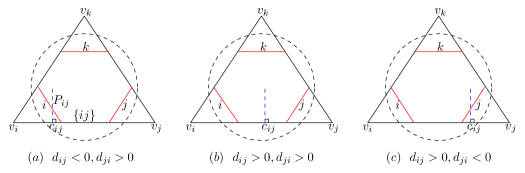
Figure 1. Poincaré dual to the ideal edge $\{ij\}\in E$ with the position determined by $d_{ij}$ and $d_{ji}$ in the Klein model (dotted). The red lines represent the boundary arcs of the ideal face $\{ijk\}$. The black triangle $v_{i}v_{j}v_{k}$ is the corresponding hyper-ideal hyperbolic triangle.

Remark 1.4.

We briefly explain the motivation of Definition 1.1 for the partial edge length on surfaces with boundary. One can refer to [16] for more details. The hyperbolic geodesic orthogonal to the hyperbolic geodesic $E_{ij}$ through $c_{ij}$ is called the edge perpendicular, denoted by $P_{ij}$. We can identify the perpendicular $P_{ij}$ with a unique 2-dimensional time-like subspace $\widetilde{P}_{ij}$ of the Lorentzian space $\mathbb{R}^{3}$ such that $\widetilde{P}_{ij}\cap\mathbb{H}^{2}=P_{ij}$. Since the 2-dimensional time-like subspaces $\widetilde{P}_{ij}$ and $\widetilde{P}_{jk}$ associated to $P_{ij}$ and $P_{jk}$ intersect in a 1-dimensional subspace of $\mathbb{R}^{3}$, then the intersection $\widetilde{P}_{ij}\cap\widetilde{P}_{jk}$ corresponds to a point $q$ in the Klein model of hyperbolic plane $\mathbb{H}^{2}$. We view this point $q$ as the intersection point of the perpendiculars $P_{ij}$ and $P_{jk}$. Note that the point $q$ may be not in $\mathbb{H}^{2}$, i.e., the perpendiculars $P_{ij},P_{jk}$ may not intersect within $\mathbb{H}^{2}$. Lemma 2.4 in [16] shows that the perpendiculars $P_{ij},P_{jk},P_{ki}$ of $\{ijk\}$ intersect at a common point $c_{ijk}$ (called face center) if and only if the condition (1) holds. Hence, the condition (1) in Definition 1.1 ensures the existence of a dual geometric structure on the Poincaré dual of an ideally triangulated surface with boundary.

Remark 1.5.

The geometric motivation for Definition 1.2 is that the vertex $v_{k}$ and face center $c_{ijk}$ of a hyper-ideal hyperbolic triangle should be in the 2-dimensional vector subspace of $\mathbb{R}^{3}$ including the vertex $\overline{v}_{k}$ of the new hyper-ideal hyperbolic triangle under the $f_{k}$-conformal variation. Please refer to [16, Remark 1.3] for more details.

The main result in [16] is the following theorem, which gives the explicit forms of the discrete conformal structures in Definition 1.2.

Theorem 1.6 ([16], Theorem 1.4).

Let $(\Sigma,\mathcal{T})$ be an ideally triangulated surface with boundary and let $d=d(f)$ be a discrete conformal structure on $(\Sigma,\mathcal{T})$. There exist constant vectors $\alpha\in\mathbb{R}^{N}$, $\eta\in\mathbb{R}_{>0}^{E}$ and $\zeta\in\mathbb{R}^{E}$ satisfying $\eta_{ij}=\eta_{ji}$ and $\zeta_{ij}=\zeta_{ji}$, such that for any right-angled hyperbolic hexagon $\{ijk\}\in F$,

(A1):

if $\frac{\sinh d_{ij}}{\sinh d_{ji}}=\sqrt{\frac{1+\alpha_{i}e^{2f_{i}}}{1+\alpha_{j}e^{2f_{j}}}}>0$, then the discrete conformal structure $d=d(f)$ is

(4) $$\coth d_{ij}=-\frac{\alpha_{i}e^{2f_{i}}}{\sinh l_{ij}}\sqrt{\frac{1+\alpha_{j}e^{2f_{j}}}{1+\alpha_{i}e^{2f_{i}}}}+\frac{\eta_{ij}e^{f_{i}+f_{j}}}{\sinh l_{ij}}$$

with

(5) $$\cosh l_{ij}=-\sqrt{(1+\alpha_{i}e^{2f_{i}})(1+\alpha_{j}e^{2f_{j}})}+\eta_{ij}e^{f_{i}+f_{j}};$$

(A2):

if $\frac{\sinh d_{ij}}{\sinh d_{ji}}=e^{\frac{1}{2}C_{ij}(f_{i}-f_{j})}>0$, then the discrete conformal structure $d=d(f)$ is

(6) $$\coth d_{ij}=\frac{\sinh(f_{j}-f_{i}-C_{ij})}{\sinh l_{ij}}+\frac{\eta_{ij}e^{f_{i}+f_{j}}}{\sinh l_{ij}}$$

with

(7) $$\cosh l_{ij}=-\cosh(f_{j}-f_{i}-C_{ij})+\eta_{ij}e^{f_{i}+f_{j}},$$

where $C\in\mathbb{R}^{E_{+}}$ is a constant vector satisfying $C_{ij}+C_{jk}+C_{ki}=0$ for any $\{ijk\}\in F$ and $C_{rs}+C_{sr}=0$ for any $\{r,s\}\subseteq\{i,j,k\}$;

(B1):

if $\frac{\sinh d_{ij}}{\sinh d_{ji}}=-\sqrt{\frac{1+\alpha_{i}e^{2f_{i}}}{1+\alpha_{j}e^{2f_{j}}}}<0$, then the discrete conformal structure $d=d(f)$ is

(8) $$\coth d_{ij}=\frac{\alpha_{i}e^{2f_{i}}}{\sinh l_{ij}}\sqrt{\frac{1+\alpha_{j}e^{2f_{j}}}{1+\alpha_{i}e^{2f_{i}}}}+\frac{\zeta_{ij}e^{f_{i}+f_{j}}}{\sinh l_{ij}}$$

with

(9) $$\cosh l_{ij}=\sqrt{(1+\alpha_{i}e^{2f_{i}})(1+\alpha_{j}e^{2f_{j}})}+\zeta_{ij}e^{f_{i}+f_{j}};$$

(B2):

if $\frac{\sinh d_{ij}}{\sinh d_{ji}}=-e^{\frac{1}{2}C_{ij}(f_{i}-f_{j})}<0$, then the discrete conformal structure $d=d(f)$ is

$$\coth d_{ij}=-\frac{\sinh(f_{j}-f_{i}-C_{ij})}{\sinh l_{ij}}+\frac{\zeta_{ij}e^{f_{i}+f_{j}}}{\sinh l_{ij}}$$

with

(10) $$\cosh l_{ij}=\cosh(f_{j}-f_{i}-C_{ij})+\zeta_{ij}e^{f_{i}+f_{j}},$$

where $C\in\mathbb{R}^{E_{+}}$ is a constant vector satisfying $C_{ij}+C_{jk}+C_{ki}=0$ for any $\{ijk\}\in F$ and $C_{rs}+C_{sr}=0$ for any $\{r,s\}\subseteq\{i,j,k\}$.

Remark 1.7.

As mentioned in [16, Remark 1.5], we can always assume $\alpha:B\rightarrow\{-1,0,1\}$ in the discrete conformal structures (A1) and (B1) and $C\equiv 0$ in the discrete conformal structures (A2) and (B2) for simplicity.

Remark 1.8.

According to [16, Remark 1.7], the discrete conformal structures (A1) and (A2) can exist alone on an ideally triangulated surface with boundary, but they can not exist simultaneously on the same ideally triangulated surface with boundary. Moreover, the discrete conformal structures (B1) and (B2) can not exist alone on an ideally triangulated surface with boundary. Therefore, we consider the mixed type of discrete conformal structures, i.e., the discrete hyperbolic metrics $l_{ij},l_{jk},l_{ki}$ of a right-angled hyperbolic hexagon $\{ijk\}\in F$ are induced by (7) and (10) or (5) and (9), such that the condition (1) holds. We call the former the mixed discrete conformal structure I and the latter the mixed discrete conformal structure II. For example, set $\{r,s,t\}=\{i,j,k\}$, if $d_{rs}<0$, then $d_{rt}<0$ by Lemma 2.17, and $d_{sr}>0,\ d_{tr}>0$ by the conditions $l_{rs}=d_{rs}+d_{sr}>0$ and $l_{rt}=d_{rt}+d_{tr}>0$ in Definition 1.1. We need $d_{st}>0,\ d_{ts}>0$ to make the condition (1) hold. Thus $l_{rs},l_{rt}$ are defined by (10) and $l_{st}$ is defined by (7) or $l_{rs},l_{rt}$ are defined by (9) and $l_{st}$ is defined by (5).

1.2. Rigidity and existence of discrete conformal structures

An important problem in discrete conformal geometry is to obtain the relationships between the discrete conformal structures and their combinatorial curvatures. The main result in this paper is the following theorem, which gives the global rigidity and existence of discrete conformal structures on ideally triangulated surfaces with boundary.

For convenience of description, we use the new parameters $\xi^{(1)}$ and $\xi^{(2)}$ to replace parameters $\eta$ and $\zeta$ in the mixed discrete conformal structures $\mathrm{I}$ and $\mathrm{II}$, respectively.

Theorem 1.9.

Let $(\Sigma,\mathcal{T})$ be an ideally triangulated surface with boundary and let $d=d(f)$ be a discrete conformal structure on $(\Sigma,\mathcal{T})$.

(i):

For the discrete conformal structure (A1), let $\alpha:B\rightarrow\{-1,0,1\}$ and $\eta\in\mathbb{R}_{>0}^{E}$ be the weights on $(\Sigma,\mathcal{T})$ satisfying $\eta_{ij}>\alpha_{i}\alpha_{j}$ if $\alpha_{i}=\alpha_{j}$ for any two adjacent boundary components $i,j\in B$;

(ii):

For the discrete conformal structure (A2), let $\eta\in\mathbb{R}_{>0}^{E}$ be the weight on $(\Sigma,\mathcal{T})$;

(iii):

For the mixed discrete conformal structure $\mathrm{I}$, i.e., the discrete hyperbolic metrics $l_{ij},l_{jk},l_{ki}$ of a right-angled hyperbolic hexagon $\{ijk\}$ are induced by (7) and (10), let $\xi^{(1)}\in\mathbb{R}_{>0}^{E}$ be the weights on $(\Sigma,\mathcal{T})$;

(iv):

For the mixed discrete conformal structure $\mathrm{II}$, i.e., the discrete hyperbolic metrics $l_{ij},l_{jk},l_{ki}$ of a right-angled hyperbolic hexagon $\{ijk\}$ are induced by (5) and (9), let $\alpha:B\rightarrow\{-1,0,1\}$ and $\xi^{(2)}:E\rightarrow(1,+\infty)$ be the weights on $(\Sigma,\mathcal{T})$;

Then the discrete conformal factor $f$ is determined by its generalized combinatorial curvature $K\in\mathbb{R}^{N}_{>0}$. In particular, the map from $f$ to $K$ is a smooth embedding. Furthermore, the image of $K$ is $\mathbb{R}^{N}_{>0}$ for the cases $\mathrm{(ii)}$ and $\mathrm{(iii)}$, for the case $\mathrm{(i)}$ if $\alpha:B\rightarrow\{0,1\}$, and for the case $\mathrm{(iv)}$ if $\alpha:B\rightarrow\{0,1\}$ and satisfies a restrictive condition.

Remark 1.10.

If $\alpha\equiv 0$, the case $\mathrm{(i)}$ in Theorem 1.9 generalizes Guo’s results [4] and Li-Xu-Zhou’s results [6]. If $\alpha\equiv 1$, the case $\mathrm{(i)}$ in Theorem 1.9 was proved by Guo-Luo [5]. Moreover, the case $\mathrm{(ii)}$ in Theorem 1.9 was also proved by Guo-Luo [5]. We include them in Theorem 1.9 for completeness. For the case $\mathrm{(iii)}$ in Theorem 1.9, the weight $\xi^{(1)}\in\mathbb{R}_{>0}^{E}$ can be extended to a wider range, please see Theorem 5.1. For the case $\mathrm{(iv)}$ in Theorem 1.9, the weight $\xi^{(2)}:E\rightarrow(1,+\infty)$ can also be extended to a wider range, and we will use a new notation $\Xi$ to denote the set of the range of weight because of its complexity, please see Subsection 6.1. Moreover, for the image of $K$ in the mixed discrete conformal structure $\mathrm{II}$, we not only require $\alpha:B\rightarrow\{0,1\}$, but also $\alpha$ satisfies a restrictive condition. Here the restrictive condition means to exclude the case that $\alpha_{j}=\alpha_{k}=1$ for a right-angled hyperbolic hexagon $\{ijk\}\in F$ with the edge lengths $l_{ij}$ and $l_{ik}$ are given by (9) and the edge length $l_{jk}$ is given by (5), please see Subsection 6.3.

1.3. Basic ideas of the proof of Theorem 1.9

The proof for the existence of discrete conformal structures uses the continuity method. We will show that the image of the curvature map is both open and closed subset of $\mathbb{R}^{N}_{>0}$, and thus is the whole space $\mathbb{R}^{N}_{>0}$. The proof for the rigidity of discrete conformal structures involves a variational principle, which was pioneered by Colin de Verdière’s work [1] for tangential circle packings on triangulated surfaces. The proof of the rigidity consists of the following three steps.

The first step is to give a characterization of the admissible space of discrete conformal factor $f$ for a right-angled hyperbolic hexagon. By a change of variables $u_{i}=u_{i}(f_{i})$ described in the proof of Lemma 2.22, the admissible space $\Omega_{ijk}$ of $f$ is transferred to the admissible space $\mathcal{U}_{ijk}$ of $u$, which is proved to be convex and simply connected. The second step is to prove the Jacobian of the generalized angles $\theta$ with respect to $u$ for a right-angled hyperbolic hexagon is symmetric and negative definite. As a consequence, the Jacobian of the generalized combinatorial curvature $K$ with respect to $u$ is symmetric and negative definite on the admissible space $\mathcal{U}=\cap\ \mathcal{U}_{ijk}$. The first step and second step enable us to define a strictly concave function on the admissible space $\mathcal{U}$. The third step is to use the following well-known result from analysis:

Lemma 1.11.

If $f:\Omega\rightarrow\mathbb{R}$ is a $C^{1}$-smooth strictly concave function on an open convex set $\Omega\subset\mathbb{R}^{n}$, then its gradient $\nabla f:\Omega\rightarrow\mathbb{R}^{n}$ is injective. Furthermore, $\nabla f$ is a smooth embedding.

The key step is how to get a change of variables $u_{i}=u_{i}(f_{i})$. For this, we need to calculate the variation formulas of the generalized angles, which is as follows.

Theorem 1.12.

Let $(\Sigma,\mathcal{T})$ be an ideally triangulated surface with boundary and let $d=d(f)$ be a discrete conformal structure on $(\Sigma,\mathcal{T})$.

(i):

For any right-angled hyperbolic hexagon $\{ijk\}\in F$,

$$\frac{\partial\theta^{jk}_{i}}{\partial f_{j}}=\frac{-1}{\sinh d_{ji}}\frac{\tanh^{\beta}h_{ij}}{\sinh l_{ij}},$$

where $\beta=1$ if $c_{ijk}$ is time-like and $\beta=-1$ if $c_{ijk}$ is space-like. If $c_{ijk}$ is light-like, we interpret the formula as $\tanh^{\beta}h_{ij}=\tanh^{\beta}h_{jk}=\tanh^{\beta}h_{ki}=1$.

(ii):

Furthermore, we have the following Glickenstein-Thomas formula for $\frac{\partial\theta^{jk}_{i}}{\partial f_{i}}$, $\frac{\partial\theta^{ik}_{j}}{\partial f_{i}}$ and $\frac{\partial\theta^{ij}_{k}}{\partial f_{i}}$, i.e.,

$$\frac{\partial\theta^{jk}_{i}}{\partial f_{i}}=\cosh l_{ij}\frac{\partial\theta^{ik}_{j}}{\partial f_{i}}+\cosh l_{ik}\frac{\partial\theta^{ij}_{k}}{\partial f_{i}}.$$

(iii):

Moreover, there is a change of variables $u_{i}=u_{i}(f_{i})$ such that

(11) $$\frac{\partial\theta^{jk}_{i}}{\partial u_{j}}=\frac{\partial\theta^{ik}_{j}}{\partial u_{i}}.$$

The function $u$ is also called a discrete conformal factor.

Here $h_{ij}$ is the signed distance of the face center $c_{ijk}$ to the hyperbolic geodesic $E_{ij}$, which is positive if $c_{ijk}$ is on the same side of the geodesic $E_{ij}$ as the right-angled hyperbolic hexagon $\{ijk\}$ and negative otherwise (or zero if $c_{ijk}$ is on the geodesic $E_{ij}$).

1.4. Organization of the paper

In Section 2, we prove Theorem 1.12 by some useful lemmas. In Section 3, we prove Theorem 1.9 (i). In Section 4, we prove Theorem 1.9 (ii). In Section 5, we prove Theorem 1.9 (iii). In Section 6, we prove Theorem 1.9 (iv).

2. Discrete conformal variations of generalized angles

In this section, we first present some basic facts in the 2-dimensional hyperbolic geometry, which are discussed in [7, Chapter 3 and 6]. Then we prove Theorem 1.12. Different from the proof of Theorem 7 in Glickenstein-Thomas [3], we are unable to get the variational formulas of generalized angle by similar geometric properties directly from the figure under the $f_{k}$-conformal variation, and we obtain them by complex calculations.

2.1. Some basic knowledge

For any vectors $x,y$ in $\mathbb{R}^{3}$, the Lorentzian inner product $*$ of $x$ and $y$ is given by $x*y=xJy^{T}$, where $J=\mathrm{diag}\{1,1,-1\}$. If $x*y=0$, then we say $x,y\in\mathbb{R}^{3}$ are Lorentz orthogonal. The Lorentzian cross product $\otimes$ of $x$ and $y$ is defined as $x\otimes y:=J(x\times y)$, where $\times$ is the Euclidean cross product.

The Lorentzian norm of $x\in\mathbb{R}^{3}$ is defined to be the complex number $||x||=\sqrt{x*x}$. Here $||x||$ is either positive, zero or positive imaginary. If $||x||$ is positive imaginary, we denote by $|||x|||$ its absolute value. Furthermore, $x\in\mathbb{R}^{3}$ is called space-like if $x*x>0$, light-like if $x*x=0$ and time-like if $x*x<0$. The hyperboloid model of $\mathbb{H}^{2}$ is defined to be

$$\mathbb{H}^{2}=\{x=(x_{1},x_{2},x_{3})\in\mathbb{R}^{3}|\ x*x=-1\ \text{and}\ x_{3}>0\},$$

which can be embedded in $(\mathbb{R}^{3},*)$. A geodesic (or hyperbolic line) in $\mathbb{H}^{2}$ is the non-empty intersection of $\mathbb{H}^{2}$ with a 2-dimensional vector subspace of $\mathbb{R}^{3}$.

The Klein model of $\mathbb{H}^{2}$ is the center projection of $\mathbb{H}^{2}$ into the plane $x_{3}=1$ of $\mathbb{R}^{3}$. In the Klein model, the interior, boundary and external points of the unit disk represent the time-like, light-like and space-like vectors respectively, and they are called hyperbolic points, ideal points and hyper-ideal points respectively. A geodesic in $\mathbb{H}^{2}$ is a chord on the unit disk. In the Klein model, a triangle $xyz$ with its three vertices $x,y,z$ being hyperbolic is called a hyperbolic triangle. If at least one of $x,y,z$ is ideal or hyper-ideal, then we say the triangle $xyz$ is a generalized hyperbolic triangle. Specially, if $x,y,z$ are all hyper-ideal, we call this triangle as a hyper-ideal hyperbolic triangle for simplicity.

The following proposition follows from the properties of Lorentzian cross product, which is used extensively in this paper.

Proposition 2.1.

Let $xyz$ be a (hyperbolic or generalized hyperbolic) triangle with $x\in\mathbb{H}^{2}$ and a right angle at $x$. Then

$$-(z*y)=(z*x)(x*y).$$

For two vectors $x,y\in\mathbb{H}^{2}$, we denoted by $d_{\mathbb{H}}(x,y)$ the hyperbolic distance between $x$ and $y$, which is the arc length of the geodesic between $x$ and $y$. We use $\mathrm{Span}(x)$ or $\mathrm{Span}(x,y)$ to denote the vector subspace spanned $x$ or $x,y$. If $x\in\mathbb{R}^{3}$ is a space-like vector, then the Lorentzian complement $x^{\bot}:=\{w\in\mathbb{R}^{3}|x*w=0\}$ of $\mathrm{Span}(x)$ is a 2-dimension vector subspace of $\mathbb{R}^{3}$ and $x^{\bot}\cap\mathbb{H}^{2}$ is non-empty. This implies that $x^{\bot}\cap\mathbb{H}^{2}$ is a geodesic in $\mathbb{H}^{2}$. And the hyperbolic distance between $x$ and $y\in\mathbb{H}^{2}$ is defined to be $d_{\mathbb{H}}(y,x^{\bot})=\inf\{d_{\mathbb{H}}(y,z)|z\in x^{\bot}\cap\mathbb{H}^{2}\}$. Let $x,y\in\mathbb{R}^{3}$ be space-like vectors. If $\mathrm{Span}(x,y)\cap\mathbb{H}^{2}$ is non-empty, then the hyperbolic distance between $x$ and $y$ is defined by $d_{\mathbb{H}}(x^{\bot},y^{\bot})=\inf\{d_{\mathbb{H}}(z,w)|z\in x^{\bot}\cap\mathbb{H}^{2},w\in y^{\bot}\cap\mathbb{H}^{2}\}$. If $\mathrm{Span}(x,y)\cap\mathbb{H}^{2}$ is empty, then $x^{\bot}$ and $y^{\bot}$ intersect in an angle $\angle(x^{\bot},y^{\bot})$ in $\mathbb{H}^{2}$.

Proposition 2.2 ([7], Chapter 3).

Suppose $x,y\in\mathbb{H}^{2}$ are time-like vectors and $z,w\in\mathbb{R}^{3}$ are space-like vectors. Then

(i):

$x*y=-|||x|||\cdot|||y|||\cosh d_{\mathbb{H}}(x,y)$;

(ii):

$|x*z|=|||x|||\cdot||z||\sinh d_{\mathbb{H}}(x,z^{\bot})$, and $x*z<0$ if and only if $x$ and $z$ are on opposite sides of the hyperplane $z^{\bot}$;

(iii):

if $\mathrm{Span}(z,w)\cap\mathbb{H}^{2}$ is non-empty, then $|z*w|=||z||\cdot||w||\cosh d_{\mathbb{H}}(z^{\bot},w^{\bot})$, and $z*w<0$ if and only if $z$ and $w$ are oppositely oriented tangent vectors of $Q$, where $Q$ is the hyperbolic line Lorentz orthogonal to $z^{\bot}$ and $w^{\bot}$;

(iv):

if $\mathrm{Span}(z,w)\cap\mathbb{H}^{2}$ is empty, then $z*w=||z||\cdot||w||\cos\angle(z^{\bot},w^{\bot})$.

The following proposition is useful for identifying perpendicular geodesics in the Klein model.

Proposition 2.3.

([8], Proposition 4) Let $x\in\mathbb{R}^{3}$ be a space-like vector and let $\gamma=x^{\bot}\cap\mathbb{H}^{2}$ be the geodesic corresponding to $x^{\bot}$. Suppose $\omega$ is another geodesic that intersects $\gamma$, and $P$ is the plane such that $\omega=P\cap\mathbb{H}^{2}$. Then $\gamma$ and $\omega$ meet at a right angle if and only if $x\in P$.

Proposition 2.4.

([7], Theorem 3.2.11) Let $P$ be a geodesic in $\mathbb{H}^{2}$ and let $y\in\mathbb{H}^{2}$ be a time-like vector. Then there exists a unique geodesic of $\mathbb{H}^{2}$ through $y$ and Lorentz orthogonal to $P$.

2.2. A geometric explanation

Consider a hyper-ideal hyperbolic triangle $v_{i}v_{j}v_{k}$ in the Kelin model. Set $\{r,s,t\}=\{i,j,k\}$. Set $E_{rs}=\mathrm{Span}(v_{r},v_{s})\cap\mathbb{H}^{2}$, then $E_{rs}$ is a geodesic in $\mathbb{H}^{2}$. Set $v_{r}^{\bot}\cap\mathbb{H}^{2}=E^{\prime}_{st}$, then $E^{\prime}_{st}$ is also a geodesic in $\mathbb{H}^{2}$ and Lorentz orthogonal to the geodesics $E_{rs},E_{rt}$. The geodesic arc in $E^{\prime}_{st}$ bounded by $E_{rs}$ and $E_{rt}$ is called a boundary arc, denoted by $r\in B$. The geodesic arc between two adjacent boundary arcs $r$ and $s$ is denoted by $\{rs\}$, which is a part of $E_{rs}$ and called an ideal edge. Moreover, the six geodesic arcs form a right-angled hyperbolic hexagon $\{ijk\}$. Conversely, for any geodesic $E_{rs}$ in $\mathbb{H}^{2}$, there exists a unique space-like vector $v^{\prime}_{t}$ such that $(v^{\prime}_{t})^{\bot}\cap\mathbb{H}^{2}=E_{rs}$. Then the three points $v^{\prime}_{i},v^{\prime}_{j}$ and $v^{\prime}_{k}$ are hyper-ideal and form a hyper-ideal hyperbolic triangle $v^{\prime}_{i}v^{\prime}_{j}v^{\prime}_{k}$, which is called the polar triangle of the hyper-ideal hyperbolic triangle $v_{i}v_{j}v_{k}$. Please refer to Figure 2.

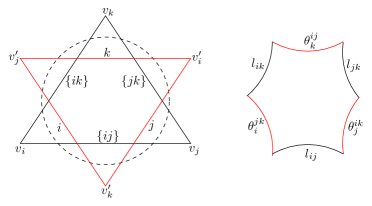
Figure 2. A hyper-ideal hyperbolic triangle $v_{i}v_{j}v_{k}$ and its polar triangle $v^{\prime}_{i}v^{\prime}_{j}v^{\prime}_{k}$ in the Kelin model (left), and a right-angled hyperbolic hexagon $\{ijk\}\in F$ in the Poincaré model (right).

By the construction of the polar triangle $v^{\prime}_{i}v^{\prime}_{j}v^{\prime}_{k}$, the vertices $v^{\prime}_{i},v^{\prime}_{j},v^{\prime}_{k}$ are determined by the vertices $v_{i},v_{j},v_{k}$ and vice versa. Without loss of generality, we assume $||v_{i}||=||v_{j}||=||v_{k}||=1$, then

(12) $$v^{\prime}_{i}=\frac{v_{k}\otimes v_{j}}{||v_{k}\otimes v_{j}||},\ v^{\prime}_{j}=\frac{v_{i}\otimes v_{k}}{||v_{i}\otimes v_{k}||},\ v^{\prime}_{k}=\frac{v_{j}\otimes v_{i}}{||v_{j}\otimes v_{i}||}.$$

Therefore, given a hyper-ideal hyperbolic triangle $v_{i}v_{j}v_{k}$, there exists a unique polar triangle $v^{\prime}_{i}v^{\prime}_{j}v^{\prime}_{k}$ with its vertices satisfying (12). The length of the ideal edge $\{rs\}\in E$ is denoted by $l_{rs}$ and the length of the boundary arc $t\in B$ is denoted by $\theta^{rs}_{t}$.

Lemma 2.5.

The vectors $c_{ijk},c_{rs},v^{\prime}_{t}$ lie in the same 2-dimensional vector subspace of $\mathbb{R}^{3}$, where the notations of $c_{ijk},c_{rs}$ follows from Remark 1.4.

Proof.

Without loss of generality, we assume $r=i,s=j,t=k$. Since $c_{ij}\in E_{ij}$, by Proposition 2.4, there exists a unique geodesic of $\mathbb{H}^{2}$ through $c_{ij}$ and Lorentz orthogonal to $E_{ij}$, which is $P_{ij}=\mathrm{Span}(c_{ij},c_{ijk})\cap\mathbb{H}^{2}$. Note that $E_{ij}=(v^{\prime}_{k})^{\bot}\cap\mathbb{H}^{2}$. By Proposition 2.3, since $E_{ij}$ and $P_{ij}$ meet at a right angle, then $v^{\prime}_{k}\in\mathrm{Span}(c_{ij},c_{ijk})$. Q.E.D.

Combining Remark 1.4 and Lemma 2.5, we have $c_{ijk}=\mathrm{Span}(v^{\prime}_{i},c_{jk})\cap\mathrm{Span}(v^{\prime}_{j},c_{ik})\cap\mathrm{Span}(v^{\prime}_{k},c_{ij})$. Due to the equivalence of $v_{i}v_{j}v_{k}$ and $v^{\prime}_{i}v^{\prime}_{j}v^{\prime}_{k}$, it is natural to consider a dual model. Note that for any $c_{ijk}\in\mathbb{R}^{3}$, $\mathrm{Span}(v_{r},c_{ijk})\cap v_{r}^{\bot}$ may not intersect within $\mathbb{H}^{2}$. For the convenience of calculations, we focus on the case that

$$\mathrm{Span}(v_{r},c_{ijk})\cap v_{r}^{\bot}\cap\mathbb{H}^{2}=\mathrm{Span}(v_{r},c_{ijk})\cap E^{\prime}_{st}\neq\emptyset,\quad\forall r\in\{i,j,k\}.$$

This condition limits the positions of $c_{ijk}$ when $c_{ijk}$ is space-like, i.e., $c_{ijk}$ can only be in some certain open domains. Denote $c^{\prime}_{st}=\mathrm{Span}(v_{r},c_{ijk})\cap E^{\prime}_{st}$ as the dual edge center, which is the unique point along the geodesic $E^{\prime}_{st}$ such that $c^{\prime}_{st}$ is of (signed) distance $\theta_{st}$ from $\{rt\}$ and $\theta_{ts}$ from $\{rs\}$. Thus we have

(13) $$\theta_{r}^{st}=\theta_{st}+\theta_{ts}.$$

Note that the signed distance $\theta_{st}$ is positive if $c^{\prime}_{st}$ is on the same side of $\{rt\}$ as $\{rs\}$ along the hyperbolic geodesic $E^{\prime}_{st}$, and negative otherwise. The above construction shows the following lemma.

Lemma 2.6.

The vectors $c_{ijk},c^{\prime}_{rs},v_{t}$ lie in the same 2-dimensional vector subspace of $\mathbb{R}^{3}$.

By Proposition 2.4, the edge perpendicular $P^{\prime}_{ij}=\mathrm{Span}(v_{k},c_{ijk})\cap\mathbb{H}^{2}$ is through $c^{\prime}_{ij}$ and Lorentz orthogonal to $E^{\prime}_{ij}$. Hence, the three edge perpendiculars $P^{\prime}_{ij},P^{\prime}_{jk},P^{\prime}_{ki}$ of $\{ijk\}$ also intersect in a point $c_{ijk}$. Similar to [16, Lemma 2.4], we further have that the three perpendiculars $P^{\prime}_{ij},P^{\prime}_{jk},P^{\prime}_{ki}$ of $\{ijk\}$ intersect in a point if and only if

(14) $$\sinh\theta_{ij}\sinh\theta_{jk}\sinh\theta_{ki}=\sinh\theta_{ji}\sinh\theta_{kj}\sinh\theta_{ik}.$$

Hence, Definition 1.1 is equivalent to the following definition with respect to the parameter $\theta$. For precision, we rewrite the boundary component $i\in B$ as $\{j^{\prime}k^{\prime}\}\in B$. We use $B_{+}$ to denote the sets of oriented boundary components and label them with ordered pairs $(j^{\prime},k^{\prime})\in B_{+}$.

Definition 2.7.

Let $(\Sigma,\mathcal{T})$ be an ideally triangulated surface with boundary. An assignment of partial edge lengths is a map $\theta:B_{+}\rightarrow\mathbb{R}$, such that $\theta_{i}^{jk}=\theta_{jk}+\theta_{kj}>0$ for each oriented boundary arc $(j^{\prime},k^{\prime})\in B_{+}$ and formula (14) holds for every right-angled hyperbolic hexagon $\{ijk\}\in F$.

Recall the definition of $h_{rs}$, which is the signed distance of the face center $c_{ijk}$ to the hyperbolic geodesic $E_{rs}$ and is positive if $c_{ijk}$ is on the same side of the geodesic $E_{rs}$ as the hyper-ideal hyperbolic triangle $v_{i}v_{j}v_{k}$ and negative otherwise (or zero if $c_{ijk}$ is on the geodesic $E_{ij}$). Similarly, we denote $q_{rs}$ as the signed distance from $c_{ijk}$ to $c^{\prime}_{rs}$, which is defined to be positive if $c_{ijk}$ is on the same side of the geodesic $E^{\prime}_{rs}$ as the polar triangle $v^{\prime}_{i}v^{\prime}_{j}v^{\prime}_{k}$ and negative otherwise (or zero if $c_{ijk}$ is on the geodesic $E^{\prime}_{rs}$). Please refer to Figure 3.

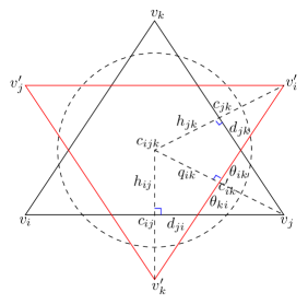
Figure 3. Data for two hyper-ideal hyperbolic triangles in the Klein model

In the Klein model, the hyper-ideal hyperbolic triangle $v_{i}v_{j}v_{k}$ and the polar triangle $v^{\prime}_{i}v^{\prime}_{j}v^{\prime}_{k}$ divide the unit disk into 13 open domains, denoted by $D_{1},D_{2},...,D_{13}$ respectively. Please refer to Figure 4.

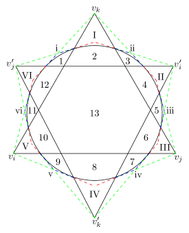
Figure 4. Division for a right-angled hyperbolic hexagon $\{ijk\}$ in the Klein model. If $c_{ijk}$ is space-like, then it can be in red and blue open domains.

By the definition of $h$ and $q$, one can directly obtain the relationships between the position of $c_{ijk}$ and the signs of $h$ and $q$ in these 13 open domains, as shown in Table 1. For example, suppose $c_{ijk}$ is in the domain $D_{1}$. Then $c_{ijk}$ is on the opposite side of $E_{ik}$ as $v_{i}v_{j}v_{k}$ and hence $h_{ik}<0$. And $c_{ijk}$ is on the same side of $E_{ij},E_{jk}$ as $v_{i}v_{j}v_{k}$ and hence $h_{ij}>0,h_{jk}>0$. Similarly, $c_{ijk}$ is also on the opposite side of $E^{\prime}_{ij}$ as $v^{\prime}_{i}v^{\prime}_{j}v^{\prime}_{k}$ and hence $q_{ij}<0$. And $c_{ijk}$ is on the same side of $E^{\prime}_{ik},E^{\prime}_{jk}$ as $v^{\prime}_{i}v^{\prime}_{j}v^{\prime}_{k}$ and hence $q_{jk}>0,q_{ik}>0$. If $c_{ijk}$ is space-like, then $c_{ijk}$ can be only in one of 12 open domains and each domain is bounded by two tangential lines and unit circle, denoted by $D_{\mathrm{I}},D_{\mathrm{II}},D_{\mathrm{III}},D_{\mathrm{IV}},D_{\mathrm{V}},D_{\mathrm{VI}}$ and $D_{\mathrm{i}},D_{\mathrm{ii}},D_{\mathrm{iii}},D_{\mathrm{iv}},D_{\mathrm{v}},D_{\mathrm{vi}}$ respectively. Please refer to Figure 4. If $c_{ijk}$ is not in one of 12 open domains, then either $\mathrm{Span}(c_{ijk},v_{r})\cap\mathbb{H}^{2}=\emptyset$ or $\mathrm{Span}(c_{ijk},v^{\prime}_{r})\cap\mathbb{H}^{2}=\emptyset$, which contradicts with the assumption that the edge centers $c_{st}\in E_{rs}$ and $c^{\prime}_{st}\in E^{\prime}_{rs}$ are in $\mathbb{H}^{2}$ for $\{r,s,t\}=\{i,j,k\}$. Similar to the case that $c_{ijk}$ is time-like, one can also directly obtain the relationships between the position of $c_{ijk}$ and the signs of $h$ and $q$ in these 12 open domains, as shown in Table 1. By moving $c_{ijk}$ to the light cone continuously, one can obtain similar results. Note that $c_{ijk}$ can only be on the unit disk that removes 12 points.

Domains	$D_{1}$($D_{\mathrm{i}}$)	$D_{2}$($D_{\mathrm{I}}$)	$D_{3}$($D_{\mathrm{ii}}$)	$D_{4}$($D_{\mathrm{II}}$)	$D_{5}$($D_{\mathrm{iii}}$)	$D_{6}$($D_{\mathrm{III}}$)	$D_{7}$($D_{\mathrm{iv}}$)	$D_{8}$($D_{\mathrm{IV}}$)	$D_{9}$($D_{\mathrm{v}}$)	$D_{10}$($D_{\mathrm{V}}$)	$D_{11}$($D_{\mathrm{vi}}$)	$D_{12}$($D_{\mathrm{VI}}$)	$D_{13}$
$h_{jk}$	+	+	-	-	-	+	+	+	+	+	+	+	+
$h_{ik}$	-	+	+	+	+	+	+	+	+	+	-	-	+
$h_{ij}$	+	+	+	+	+	+	-	-	-	+	+	+	+
$q_{jk}$	+	+	+	+	+	+	+	+	-	-	-	+	+
$q_{ik}$	+	+	+	+	-	-	-	+	+	+	+	+	+
$q_{ij}$	-	-	-	+	+	+	+	+	+	+	+	+	+

Table 1. Relationships between the position of $c_{ijk}$ and the signs of $h$ and $q$

In the following, we provide another way to obtain Table 1. Suppose $c_{ijk}$ is time-like. Without loss of generality, we assume $c_{ijk}$ is in the domain $D_{1}$. By Lemma 2.5, the vectors $c_{ijk},c_{ik},v^{\prime}_{j}$ lie in the same 2-dimensional vector subspace of $\mathbb{R}^{3}$. Due to $c_{ijk}$ is not in the polar triangle $v^{\prime}_{i}v^{\prime}_{j}v^{\prime}_{k}$, then $c_{ik}\in E_{ik}$ is not in $\{ik\}$. Furthermore, since $c_{ijk}$ is in $D_{1}$, then $c_{ik}$ is on the opposite side of $k$ as $i$. By the definition of $d$ in Remark 1.3, we have $d_{ki}<0,d_{ik}>0$. Similarly, we have $d_{kj}<0,d_{jk}>0,d_{ij}>0,d_{ji}>0$. By Lemma 2.6, the vectors $c_{ijk},c^{\prime}_{ij},v_{k}$ lie in the same 2-dimensional vector subspace of $\mathbb{R}^{3}$. Due to $c_{ijk}$ is not in the hyper-ideal hyperbolic triangle $v_{i}v_{j}v_{k}$, then $c^{\prime}_{ij}\in E^{\prime}_{ij}$ is not in $k$. Furthermore, since $c_{ijk}$ is in $D_{1}$, then $c^{\prime}_{ij}$ is on the opposite side of $\{ik\}$ as $\{jk\}$ and hence $\theta_{ji}<0,\theta_{ij}>0$. Similarly, we have $\theta_{jk}<0,\theta_{kj}>0,\theta_{ik}>0,\theta_{ki}>0$. By Corollary 2.11, we have $h_{ik}<0,h_{jk}>0,h_{ij}>0$ and $q_{ij}<0,q_{ik}>0,q_{jk}>0$. The case that $c_{ijk}$ is space-like follows from the following two lemmas.

Lemma 2.8.

The signs of $q$ and $h$ in the domains $D_{\mathrm{I}},D_{\mathrm{II}},D_{\mathrm{III}},D_{\mathrm{IV}},D_{\mathrm{V}},D_{\mathrm{VI}}$ are the same as those in the domains $D_{2},D_{4},D_{6},D_{8},D_{10},D_{12}$, respectively.

Proof.

We only prove the signs of $q$ and $h$ in the domain $D_{\mathrm{V}}$ are the same as those in the domain $D_{10}$, and the remaining cases are similar.

If $c_{ijk}$ is in the domain $D_{10}$, then $q_{jk}<0$ and the rest is positive by Table 1. Suppose $c_{ijk}$ is in the domain $D_{\mathrm{V}}$. By Lemma 2.5, the vectors $c_{ijk},c_{ij},v^{\prime}_{k}$ lie in the same 2-dimensional vector subspace of $\mathbb{R}^{3}$. Due to $c_{ijk}$ is not in the polar triangle $v^{\prime}_{i}v^{\prime}_{j}v^{\prime}_{k}$, then $c_{ij}\in E_{ij}$ is not in $\{ij\}$. Furthermore, since $c_{ijk}$ is in $D_{\mathrm{V}}$, then $c_{ij}$ is on the opposite side of $j$ as $i$ and hence $d_{ij}<0,d_{ji}>0$. Similarly, we have $d_{ik}<0,d_{ki}>0,d_{jk}>0,d_{kj}>0$. By Proposition 2.12, we have $h_{ij}>0,h_{jk}>0,h_{ik}>0$. Note that $c_{ijk}$ is in the polar triangle $v^{\prime}_{i}v^{\prime}_{j}v^{\prime}_{k}$. By Lemma 2.6, the vectors $c_{ijk},c^{\prime}_{rs},v_{t}$ lie in the same 2-dimensional vector subspace of $\mathbb{R}^{3}$ for $\{r,s,t\}=\{i,j,k\}$. Then $c^{\prime}_{rs}\in E^{\prime}_{rs}$ is in $t$. Hence, $\theta_{ij}>0,\theta_{ji}>0,\theta_{jk}<0,\theta_{kj}>0,\theta_{ik}>0,\theta_{ki}>0$. By Proposition 2.12, we have $q_{ij}>0,q_{jk}<0,q_{ik}>0$. Q.E.D.

Lemma 2.9.

The signs of $q$ and $h$ in the domains $D_{\mathrm{i}},D_{\mathrm{ii}},D_{\mathrm{iii}},D_{\mathrm{iv}},D_{\mathrm{v}},D_{\mathrm{vi}}$ are the same as those in the domains $D_{1},D_{3},D_{5},D_{7},D_{9},D_{11}$, respectively.

Proof.

We only prove the signs of $q$ and $h$ in the domain $D_{\mathrm{vi}}$ are the same as those in the domain $D_{11}$, and the remaining cases are similar.

If $c_{ijk}$ is in the domain $D_{11}$, then $q_{i}<0,h_{j}<0$ and the rest is positive by Table 1. Suppose $c_{ijk}$ is in the domain $D_{\mathrm{vi}}$. By Lemma 2.5, the vectors $c_{ijk},c_{ij},v^{\prime}_{k}$ lie in the same 2-dimensional vector subspace of $\mathbb{R}^{3}$. Due to $c_{ijk}$ is not in the polar triangle $v^{\prime}_{i}v^{\prime}_{j}v^{\prime}_{k}$, then $c_{ij}\in E_{ij}$ is not in $\{ij\}$. Furthermore, since $c_{ijk}$ is in $D_{\mathrm{vi}}$, then $c_{ij}$ is on the opposite side of $j$ as $i$ and hence $d_{ij}<0,d_{ji}>0$. Similarly, we have $d_{ik}<0,d_{ki}>0,d_{jk}>0,d_{kj}>0$. By Proposition 2.14, we have $h_{ij}<0,h_{jk}>0,h_{ik}>0$. By Lemma 2.6, the vectors $c_{ijk},c^{\prime}_{jk},v_{i}$ lie in the same 2-dimensional vector subspace of $\mathbb{R}^{3}$. Due to $c_{ijk}$ is not in the hyper-ideal hyperbolic triangle $v_{i}v_{j}v_{k}$, then $c^{\prime}_{jk}\in E^{\prime}_{jk}$ is not in $i$. Furthermore, since $c_{ijk}$ is in $D_{\mathrm{vi}}$, then $c^{\prime}_{jk}$ is on the opposite side of $\{ik\}$ as $\{ij\}$ and hence $\theta_{jk}<0,\theta_{kj}>0$. Similarly, we have $\theta_{ji}<0,\theta_{ij}>0,\theta_{ik}>0,\theta_{ki}>0$. By Proposition 2.14, we have $q_{ij}>0,q_{jk}<0,q_{ik}>0$. Q.E.D.

By direct calculations, we can get the following results. As the proofs of the Lemma 2.10, Proposition 2.12 and Proposition 2.14 are too long, we defer them to Appendix A. For simplicity, we set $h_{t}=h_{rs},\ q_{t}=q_{rs}$ for $\{r,s,t\}=\{i,j,k\}$.

Lemma 2.10.

If $c_{ijk}$ is time-like, then

$$\sinh q_{r}=\cosh h_{s}\cdot\sinh d_{rt}=\cosh h_{t}\cdot\sinh d_{rs},$$

$$\sinh h_{r}=\cosh q_{s}\cdot\sinh\theta_{rt}=\cosh q_{t}\cdot\sinh\theta_{rs}.$$

As a direct corollary of Lemma 2.10, we have

Corollary 2.11.

If $c_{ijk}$ is time-like, then the signs of $q_{r}$, $d_{rt}$ and $d_{rs}$ are the same and the signs of $h_{r}$, $\theta_{rs}$ and $\theta_{rt}$ are the same.

Proposition 2.12.

If $c_{ijk}\in\mathbb{R}^{3}$ lies in the open domain $D_{\mathrm{V}}$, then

$$\cosh q_{i}=-\sinh h_{j}\cdot\sinh d_{ik}=-\sinh h_{k}\cdot\sinh d_{ij},$$

$$\cosh q_{j}=\sinh h_{i}\cdot\sinh d_{jk}=\sinh h_{k}\cdot\sinh d_{ji},$$

$$\cosh q_{k}=\sinh h_{i}\cdot\sinh d_{kj}=\sinh h_{j}\cdot\sinh d_{ki},$$

$$\cosh h_{i}=\sinh q_{j}\cdot\sinh\theta_{ik}=\sinh q_{k}\cdot\sinh\theta_{ij},$$

$$\cosh h_{j}=-\sinh q_{i}\cdot\sinh\theta_{jk}=\sinh q_{k}\cdot\sinh\theta_{ji},$$

$$\cosh h_{k}=-\sinh q_{i}\cdot\sinh\theta_{kj}=\sinh q_{j}\cdot\sinh\theta_{ki}.$$

If $c_{ijk}\in\mathbb{R}^{3}$ lies in the open domain $D_{\mathrm{II}}$, then we swap $h$ and $q$, and $\theta$ and $d$.

If $c_{ijk}$ lies in the domains $D_{\mathrm{I}},D_{\mathrm{III}},D_{\mathrm{IV}}$ or $D_{\mathrm{VI}}$, we have similar propositions. Using these propositions, we can prove Lemma 2.8 and further obtain Table 1. Moreover, from Table 1, we see that $c_{ijk}$ lies in the open domains $D_{\mathrm{I}},D_{\mathrm{II}},D_{\mathrm{III}},D_{\mathrm{IV}},D_{\mathrm{V}}$ or $D_{\mathrm{VI}}$ if and only if one of $q_{i},q_{j},q_{k},h_{i},h_{j},h_{k}$ is negative and the others are positive. Hence, these propositions can be written as a unified form.

Lemma 2.13.

Let $c_{ijk}\in\mathbb{R}^{3}$ lie in one of the open domains $D_{\mathrm{I}},D_{\mathrm{II}},D_{\mathrm{III}},D_{\mathrm{IV}},D_{\mathrm{V}},D_{\mathrm{VI}}$. If $q_{r}<0$, then

$$\cosh q_{r}=-\sinh h_{s}\cdot\sinh d_{rt}=-\sinh h_{t}\cdot\sinh d_{rs},$$

$$\cosh q_{s}=\sinh h_{r}\cdot\sinh d_{st}=\sinh h_{t}\cdot\sinh d_{sr},$$

$$\cosh q_{t}=\sinh h_{r}\cdot\sinh d_{ts}=\sinh h_{s}\cdot\sinh d_{tr},$$

$$\cosh h_{r}=\sinh q_{s}\cdot\sinh\theta_{rt}=\sinh q_{t}\cdot\sinh\theta_{rs},$$

$$\cosh h_{s}=-\sinh q_{r}\cdot\sinh\theta_{st}=\sinh q_{t}\cdot\sinh\theta_{sr},$$

$$\cosh h_{t}=-\sinh q_{r}\cdot\sinh\theta_{ts}=\sinh q_{s}\cdot\sinh\theta_{tr}.$$

If $h_{r}<0$, then we swap $h,\ \theta$ and $q,\ d$.

Proposition 2.14.

Let $c_{ijk}\in\mathbb{R}^{3}$ lie in the open domain $D_{\mathrm{vi}}$, then

$$\cosh q_{i}=\sinh h_{j}\cdot\sinh d_{ik}=-\sinh h_{k}\cdot\sinh d_{ij},$$

$$\cosh q_{j}=\sinh h_{i}\cdot\sinh d_{jk}=\sinh h_{k}\cdot\sinh d_{ji},$$

$$\cosh q_{k}=\sinh h_{i}\cdot\sinh d_{kj}=-\sinh h_{j}\cdot\sinh d_{ki},$$

$$\cosh h_{i}=\sinh q_{j}\cdot\sinh\theta_{ik}=\sinh q_{k}\cdot\sinh\theta_{ij},$$

$$\cosh h_{j}=\sinh q_{i}\cdot\sinh\theta_{jk}=-\sinh q_{k}\cdot\sinh\theta_{ji},$$

$$\cosh h_{k}=-\sinh q_{i}\cdot\sinh\theta_{kj}=\sinh q_{j}\cdot\sinh\theta_{ki}.$$

Similarly, if $c_{ijk}$ lies in the domains $D_{\mathrm{i}},D_{\mathrm{ii}},D_{\mathrm{iii}},D_{\mathrm{iv}}$ or $D_{\mathrm{v}}$, we have the corresponding propositions. Using these propositions, we can prove Lemma 2.9 and further obtain Table 1. Moreover, from Table 1, we see that $c_{ijk}$ lies in the open domains $D_{\mathrm{i}},D_{\mathrm{ii}},D_{\mathrm{iii}},D_{\mathrm{iv}},D_{\mathrm{v}}$ or $D_{\mathrm{vi}}$ if and only if $q_{r}<0,h_{s}<0$ and the rest are positive. Hence, these propositions can also be written as a unified form.

Lemma 2.15.

Let $c_{ijk}\in\mathbb{R}^{3}$ lie in one of the open domains $D_{\mathrm{i}},D_{\mathrm{ii}},D_{\mathrm{iii}},D_{\mathrm{iv}},D_{\mathrm{v}},D_{\mathrm{vi}}$. If $q_{r}<0,h_{s}<0$, then

$$\cosh q_{r}=\sinh h_{s}\cdot\sinh d_{rt}=-\sinh h_{t}\cdot\sinh d_{rs},$$

$$\cosh q_{s}=\sinh h_{r}\cdot\sinh d_{st}=\sinh h_{t}\cdot\sinh d_{sr},$$

$$\cosh q_{t}=\sinh h_{r}\cdot\sinh d_{ts}=-\sinh h_{s}\cdot\sinh d_{tr},$$

$$\cosh h_{r}=\sinh q_{s}\cdot\sinh\theta_{rt}=\sinh q_{t}\cdot\sinh\theta_{rs},$$

$$\cosh h_{s}=\sinh q_{r}\cdot\sinh\theta_{st}=-\sinh q_{t}\cdot\sinh\theta_{sr},$$

$$\cosh h_{t}=-\sinh q_{r}\cdot\sinh\theta_{ts}=\sinh q_{s}\cdot\sinh\theta_{tr}.$$

As a direct corollary of Lemma 2.13 and Lemma 2.15, we have

Corollary 2.16.

If $c_{ijk}$ is space-like, then the signs of $q_{r}$, $d_{rt}$ and $d_{rs}$ are the same and the signs of $h_{r}$, $\theta_{rs}$ and $\theta_{rt}$ are the same.

Combining Corollary 2.11 and Corollary 2.16 gives the following lemma.

Lemma 2.17.

For any right-angled hyperbolic hexagon $\{ijk\}\in F$, the signs of $q_{r}$, $d_{rt}$ and $d_{rs}$ are the same and the signs of $h_{r}$, $\theta_{rs}$ and $\theta_{rt}$ are the same.

Proof.

If $c_{ijk}$ is time-like, the conclusion follows from Corollary 2.11. If $c_{ijk}$ is space-like, the conclusion follows from Corollary 2.16. If $c_{ijk}$ is light-like, the conclusion follows from continuity by moving the center to the light cone. Q.E.D.

2.3. Variational formulas of generalized angle

We divide Theorem 1.12 into Lemma 2.18, Lemma 2.20 and Lemma 2.22, and prove them respectively.

Lemma 2.18.

For a right-angled hyperbolic hexagon $\{ijk\}\in F$, we have

(15) $$\frac{\partial\theta^{jk}_{i}}{\partial f_{j}}=\frac{-1}{\sinh d_{ji}}\frac{\tanh^{\beta}h_{ij}}{\sinh l_{ij}},$$

where $\beta=1$ if $c_{ijk}$ is time-like and $\beta=-1$ if $c_{ijk}$ is space-like. If $c_{ijk}$ is light-like, we interpret the formula as $\tanh^{\beta}h_{ij}=\tanh^{\beta}h_{jk}=\tanh^{\beta}h_{ki}=1$.

Proof.

Without loss of generality, we assume $||v_{i}||=||v_{j}||=||v_{k}||=1$ and $||c_{ijk}||^{2}=\pm 1$. For simplicity, we set $l_{r}=l_{st},\ \theta_{r}=\theta^{st}_{r},\ h_{r}=h_{st},\ q_{r}=q_{st}$ and $A=\sinh l_{r}\sinh l_{s}\sinh\theta_{t}$, where $\{r,s,t\}=\{i,j,k\}$. By generalized hyperbolic cosine law, i.e., $\cosh l_{r}=\cosh\theta_{r}\sinh l_{s}\sinh l_{t}-\cosh l_{s}\cosh l_{t}$, we have

(16) $$\frac{\partial\theta_{i}}{\partial l_{i}}=\frac{\sinh l_{i}}{A},\ \frac{\partial\theta_{i}}{\partial l_{j}}=-\frac{\sinh l_{i}\cosh\theta_{k}}{A},\ \frac{\partial\theta_{i}}{\partial l_{k}}=-\frac{\sinh l_{i}\cosh\theta_{j}}{A}.$$

By (2) and (3), we have

(17) $$\frac{\partial\theta_{i}}{\partial f_{j}}= \frac{\partial\theta_{i}}{\partial l_{i}}\frac{\partial l_{i}}{\partial f_{j}}+\frac{\partial\theta_{i}}{\partial l_{j}}\frac{\partial l_{j}}{\partial f_{j}}+\frac{\partial\theta_{i}}{\partial l_{k}}\frac{\partial l_{k}}{\partial f_{j}}$$

$$= \frac{\sinh l_{i}}{A}\cdot\coth d_{jk}+\frac{-\sinh l_{i}\cosh\theta_{j}}{A}\cdot\coth d_{ji}$$

$$= \frac{1}{\sinh l_{k}\sinh\theta_{j}}\cdot\left(\coth d_{jk}-\cosh\theta_{j}\cdot\coth d_{ji}\right)$$

$$= \frac{1}{\sinh l_{k}\sinh\theta_{j}}\cdot\left[\coth d_{jk}-\cosh(\theta_{ki}+\theta_{ik})\cdot\coth d_{ji}\right]$$

$$= \frac{1}{\sinh l_{k}\sinh\theta_{j}}\cdot(\coth d_{jk}-\cosh\theta_{ki}\cosh\theta_{ik}\coth d_{ji}$$

$$\ \ \ \ \ \ \ \ \ \ \ \ \ \ \ \ \ \ \ \ \ \ \ \ \ \ \ \ -\sinh\theta_{ki}\sinh\theta_{ik}\coth d_{ji}),$$

where (13) is used in the forth line. Set

(18) $$L_{1}=\coth d_{jk}-\cosh\theta_{ki}\cosh\theta_{ik}\coth d_{ji},\ L_{2}=-\sinh\theta_{ki}\sinh\theta_{ik}\coth d_{ji}.$$

Then

(19) $$\frac{\partial\theta_{i}}{\partial f_{j}}=\frac{1}{\sinh l_{k}\sinh\theta_{j}}\cdot(L_{1}+L_{2}).$$

To calculate $L_{1}$ and $L_{2}$, we first give some formulas. Please refer to Figure 3. Applying Proposition 2.1 to the generalized right-angled hyperbolic triangle $c_{ijk}c_{ij}v_{j}$ gives

(20) $$v_{j}\ast c_{ijk}=-(c_{ij}\ast c_{ijk})(v_{j}\ast c_{ij})=\sinh d_{ji}\cdot(c_{ij}\ast c_{ijk}),$$

where $v_{j}\ast c_{ij}=-\sinh d_{ji}$ follows from Proposition 2.2 (ii). Similarly, in the generalized right-angled hyperbolic triangle $c_{ijk}c_{jk}v_{j}$, we have

(21) $$v_{j}\ast c_{ijk}=-(v_{j}\ast c_{jk})(c_{jk}\ast c_{ijk})=\sinh d_{jk}\cdot(c_{jk}\ast c_{ijk}),$$

where $v_{j}\ast c_{jk}=-\sinh d_{jk}$ follows from Proposition 2.2 (ii). Combining (20) and (21) gives

(22) $$\sinh d_{ji}\cdot(c_{ij}\ast c_{ijk})=\sinh d_{jk}\cdot(c_{jk}\ast c_{ijk}).$$

By Proposition 2.2 $\mathrm{(iii)}$, we have $(c_{ijk}\otimes v_{j})\ast(v_{j}\otimes c_{jk})=||v_{j}\otimes c_{ijk}||\cdot||v_{j}\otimes c_{jk}||(-\cosh\theta_{ik}).$ Moreover,

$$(c_{ijk}\otimes v_{j})\ast(v_{j}\otimes c_{jk})=(c_{jk}\ast c_{ijk})||v_{j}||^{2}-(v_{j}\ast c_{ijk})(v_{j}\ast c_{jk})=(c_{jk}\ast c_{ijk})\cdot\cosh^{2}d_{jk},$$

where (21) is used in the second equality. Since $||v_{j}\otimes c_{jk}||^{2}=(v_{j}\ast c_{jk})^{2}+1=\cosh^{2}d_{jk}$, then

(23) $$\cosh\theta_{ik}=-\frac{(c_{ijk}\otimes v_{j})\ast(v_{j}\otimes c_{jk})}{||v_{j}\otimes c_{ijk}||\cdot||v_{j}\otimes c_{jk}||}=-\frac{(c_{jk}\ast c_{ijk})\cdot\cosh d_{jk}}{||v_{j}\otimes c_{ijk}||}.$$

Similarly, $(c_{ijk}\otimes v_{j})\ast(v_{j}\otimes c_{ij})=||v_{j}\otimes c_{ijk}||\cdot||v_{j}\otimes c_{ij}||(-\cosh\theta_{ki}).$ Moreover,

$$(c_{ijk}\otimes v_{j})\ast(v_{j}\otimes c_{ij})=(c_{ij}\ast c_{ijk})||v_{j}||^{2}-(v_{j}\ast c_{ijk})(v_{j}\ast c_{ij})=(c_{ij}\ast c_{ijk})\cdot\cosh^{2}d_{ji},$$

where (20) is used in the second equality. Since $||v_{j}\otimes c_{ij}||^{2}=(v_{j}\ast c_{ij})^{2}+1=\cosh^{2}d_{ji}$, then

(24) $$\cosh\theta_{ki}=-\frac{(c_{ijk}\otimes v_{j})\ast(v_{j}\otimes c_{ij})}{||v_{j}\otimes c_{ijk}||\cdot||v_{j}\otimes c_{ij}||}=-\frac{(c_{ij}\ast c_{ijk})\cdot\cosh d_{ji}}{||v_{j}\otimes c_{ijk}||}.$$

By the properties of Lorentzian cross product, we have

(25) $$||v_{j}\otimes c_{ijk}||^{2}=(v_{j}\otimes c_{ijk})*(v_{j}\otimes c_{ijk})=(v_{j}\ast c_{ijk})^{2}-||c_{ijk}||^{2},$$

and

(26) $$||c_{ij}\otimes c_{ijk}||^{2}=(c_{ij}\otimes c_{ijk})*(c_{ij}\otimes c_{ijk})=(c_{ij}\ast c_{ijk})^{2}+||c_{ijk}||^{2}.$$

Adding (25) and (26) gives

(27) $$||v_{j}\otimes c_{ijk}||^{2}+||c_{ij}\otimes c_{ijk}||^{2}= (v_{j}\ast c_{ijk})^{2}+(c_{ij}\ast c_{ijk})^{2}$$

$$= (c_{ij}\ast c_{ijk})^{2}\cdot\sinh^{2}d_{ji}+(c_{ij}\ast c_{ijk})^{2}$$

$$= (c_{ij}\ast c_{ijk})^{2}\cosh^{2}d_{ji},$$

where (20) is used in the second line. Then

(28) $$\sinh^{2}\theta_{ki}= \cosh^{2}\theta_{ki}-1$$

$$= \frac{1}{||v_{j}\otimes c_{ijk}||^{2}}[(c_{ij}\ast c_{ijk})^{2}\cosh^{2}d_{ji}-||v_{j}\otimes c_{ijk}||^{2}]$$

$$= \frac{||c_{ij}\otimes c_{ijk}||^{2}}{||v_{j}\otimes c_{ijk}||^{2}},$$

where (24) is used in the second line and (27) is used in the last line.

Now we begin to calculate $L_{1}$ and $L_{2}$ in (18).

$$L_{2}= -\sinh\theta_{ki}\sinh\theta_{ik}\cdot\coth d_{ji}$$

$$= -\sinh\theta_{ki}\cdot\sinh\theta_{ik}\cdot\frac{\cosh d_{ji}}{\sinh d_{ji}}\cdot\frac{||v_{j}\otimes c_{ijk}||}{c_{ij}\ast c_{ijk}}\cdot\frac{c_{ij}\ast c_{ijk}}{||v_{j}\otimes c_{ijk}||}$$

$$= \sinh\theta_{ki}\sinh\theta_{ik}\cdot\frac{||v_{j}\otimes c_{ijk}||}{(c_{ij}\ast c_{ijk})\sinh d_{ji}}\cdot\cosh\theta_{ki},$$

where (24) is used in the last line.

$$L_{1}= \coth d_{jk}-\cosh\theta_{ki}\cosh\theta_{ik}\cdot\coth d_{ji}$$

$$= \frac{\cosh d_{jk}\cdot(c_{jk}\ast c_{ijk})}{\sinh d_{ji}\cdot(c_{ij}\ast c_{ijk})}+\frac{(c_{ij}\ast c_{ijk})\cosh d_{ji}}{||v_{j}\otimes c_{ijk}||}\cdot\cosh\theta_{ik}\cdot\frac{\cosh d_{ji}}{\sinh d_{ji}}$$

$$= \frac{\cosh\theta_{ik}}{\sinh d_{ji}\cdot(c_{ij}\ast c_{ijk})\cdot||v_{j}\otimes c_{ijk}||}\big{(}-||v_{j}\otimes c_{ijk}||^{2}+(c_{ij}\ast c_{ijk})^{2}\cosh^{2}d_{ji}\big{)}$$

$$= \frac{\cosh\theta_{ik}\cdot||c_{ij}\otimes c_{ijk}||^{2}}{\sinh d_{ji}\cdot(c_{ij}\ast c_{ijk})\cdot||v_{j}\otimes c_{ijk}||}$$

$$= \frac{\cosh\theta_{ik}\sinh^{2}\theta_{ki}||v_{j}\otimes c_{ijk}||}{\sinh d_{ji}(c_{ij}\ast c_{ijk})},$$

where (22) and (24) are used in the second line, (23) is used in the third line, (27) is used in the forth line, and (28) is used in the last line. Therefore, the formula (19) can be written as

$$\frac{\partial\theta_{i}}{\partial f_{j}}= \frac{1}{\sinh l_{k}\sinh\theta_{j}}\cdot(L_{1}+L_{2})$$

$$= \frac{1}{\sinh l_{k}\sinh\theta_{j}}\cdot\frac{\sinh\theta_{ki}\cdot||v_{j}\otimes c_{ijk}||}{(c_{ij}\ast c_{ijk})\sinh d_{ji}}\cdot(\cosh\theta_{ik}\sinh\theta_{ki}+\sinh\theta_{ik}\cosh\theta_{ki})$$

$$= \frac{1}{\sinh l_{k}\sinh\theta_{j}}\cdot\frac{\sinh\theta_{ki}\cdot||v_{j}\otimes c_{ijk}||}{(c_{ij}\ast c_{ijk})\sinh d_{ji}}\cdot\sinh\theta_{j}$$

$$= \frac{1}{\sinh l_{k}\sinh d_{ji}}\cdot\frac{\sinh\theta_{ki}\cdot||v_{j}\otimes c_{ijk}||}{c_{ij}\ast c_{ijk}}.$$

(i): Suppose $c_{ijk}$ is time-like, then $||c_{ijk}||^{2}=-1$ and $v_{j}*c_{ijk}=-\sinh q_{j}$. By (25), we have $||v_{j}\otimes c_{ijk}||=\cosh q_{j}$. Then $\sinh\theta_{ki}\cdot||v_{j}\otimes c_{ijk}||=\sinh\theta_{ki}\cdot\cosh q_{j}=\sinh h_{k}$ by Lemma 2.10. Since $c_{ij}\ast c_{ijk}=-\cosh h_{k}$, then

$$\frac{\partial\theta_{i}}{\partial f_{j}}=\frac{1}{\sinh d_{ji}\sinh l_{k}}\cdot\frac{\sinh h_{k}}{-\cosh h_{k}}=\frac{-1}{\sinh d_{ji}}\frac{\tanh h_{k}}{\sinh l_{k}}.$$

(ii): Suppose $c_{ijk}$ is space-like, then $||c_{ijk}||^{2}=1$ and $v_{j}*c_{ijk}=\pm\cosh q_{j}$, thus $||v_{j}\otimes c_{ijk}||=\sinh q_{j}$ if $q_{j}>0$ and $||v_{j}\otimes c_{ijk}||=-\sinh q_{j}$ if $q_{j}<0$ by (25).

If $c_{ijk}$ is in one of the domains $D_{\mathrm{I}},D_{\mathrm{II}},D_{\mathrm{V}},D_{\mathrm{VI}}$, then $q_{j}>0$ and $h_{k}>0$ by Table 1. Then $\sinh\theta_{ki}\cdot||v_{j}\otimes c_{ijk}||=\sinh\theta_{ki}\cdot\sinh q_{j}=\cosh h_{k}$ by Lemma 2.13. And $c_{ij}\ast c_{ijk}=-\sinh h_{k}$.

If $c_{ijk}$ is in the domain $D_{\mathrm{III}}$, then $q_{j}<0$ and $h_{k}>0$ by Table 1. Then $\sinh\theta_{ki}\cdot||v_{j}\otimes c_{ijk}||=\sinh\theta_{ki}\cdot(-\sinh q_{j})=\cosh h_{k}$ by Lemma 2.13. And $c_{ij}\ast c_{ijk}=-\sinh h_{k}$.

If $c_{ijk}$ is in the domain $D_{\mathrm{IV}}$, then $q_{j}>0$ and $h_{k}<0$ by Table 1. Then $\sinh\theta_{ki}\cdot||v_{j}\otimes c_{ijk}||=\sinh\theta_{ki}\cdot\sinh q_{j}=-\cosh h_{k}$ by Lemma 2.13. Note that $c_{ij}\ast c_{ijk}=-\sinh(d_{\mathbb{H}}(c_{ij},(c_{ijk})^{\bot}))=-\sinh(-h_{k})=\sinh h_{k}$.

If $c_{ijk}$ is in one of the domains $D_{\mathrm{i}},D_{\mathrm{ii}},D_{\mathrm{vi}}$, then $q_{j}>0$ and $h_{k}>0$ by Table 1. Then $\sinh\theta_{ki}\cdot||v_{j}\otimes c_{ijk}||=\sinh\theta_{ki}\cdot\sinh q_{j}=\cosh h_{k}$ by Lemma 2.15. And $c_{ij}\ast c_{ijk}=-\sinh h_{k}$.

If $c_{ijk}$ is in the domain $D_{\mathrm{iii}}$, then $q_{j}<0$ and $h_{k}>0$ by Table 1. Then $\sinh\theta_{ki}\cdot||v_{j}\otimes c_{ijk}||=\sinh\theta_{ki}\cdot(-\sinh q_{j})=\cosh h_{k}$ Lemma 2.15. And $c_{ij}\ast c_{ijk}=-\sinh h_{k}$.

If $c_{ijk}$ is in the domain $D_{\mathrm{v}}$, then $q_{j}>0$ and $h_{k}<0$ by Table 1. Then $\sinh\theta_{ki}\cdot||v_{j}\otimes c_{ijk}||=\sinh\theta_{ki}\cdot\sinh q_{j}=-\cosh h_{k}$ by Lemma 2.15. And $c_{ij}\ast c_{ijk}=\sinh h_{k}$.

If $c_{ijk}$ is in the domain $D_{\mathrm{iv}}$, then $q_{j}<0$ and $h_{k}<0$ by Table 1. Then $\sinh\theta_{ki}\cdot||v_{j}\otimes c_{ijk}||=\sinh\theta_{ki}\cdot(-\sinh q_{j})=-\cosh h_{k}$ by Lemma 2.15. And $c_{ij}\ast c_{ijk}=\sinh h_{k}$.

In summary, if $c_{ijk}$ is space-like, then

$$\frac{\partial\theta_{i}}{\partial f_{j}}=\frac{-1}{\sinh d_{ji}}\frac{\coth h_{k}}{\sinh l_{k}}.$$

(iii): The case that $c_{ijk}$ is light-like follows from continuity by moving the center to the light cone. In fact, if $c_{ijk}$ is light-like, then $||c_{ijk}||^{2}=0$. Combining (28) and (26) gives

$$\frac{\sinh^{2}\theta_{ki}\cdot||v_{j}\otimes c_{ijk}||^{2}}{(c_{ij}\ast c_{ijk})^{2}}=\frac{||c_{ij}\otimes c_{ijk}||^{2}}{(c_{ij}\ast c_{ijk})^{2}}=1.$$

Since $||c_{ij}\otimes c_{ijk}||=-(c_{ij}\ast c_{ijk})$, then

$$\frac{\partial\theta_{i}}{\partial f_{j}}=\frac{-1}{\sinh d_{ji}\sinh l_{k}}.$$

This completes the proof. Q.E.D.

Remark 2.19.

Actually, the formulas in the proof of Lemma 2.18 are the sine and cosine laws of generalized right-angled hyperbolic triangles. In order to avoid discussing one by one, we use Lorentzian inner product and Lorentzian cross product to unify calculations.

Lemma 2.20.

For a right-angled hyperbolic hexagon $\{ijk\}\in F$, we have

(29) $$\frac{\partial\theta^{jk}_{i}}{\partial f_{i}}=\cosh l_{ij}\frac{\partial\theta^{ik}_{j}}{\partial f_{i}}+\cosh l_{ik}\frac{\partial\theta^{ij}_{k}}{\partial f_{i}}.$$

Proof.

Under the same notations as in the proof of Lemma 2.18, a routine calculation gives

$$\frac{\partial\theta_{i}}{\partial f_{i}}= \frac{\partial\theta_{i}}{\partial l_{i}}\frac{\partial l_{i}}{\partial f_{i}}+\frac{\partial\theta_{i}}{\partial l_{j}}\frac{\partial l_{j}}{\partial f_{i}}+\frac{\partial\theta_{i}}{\partial l_{k}}\frac{\partial l_{k}}{\partial f_{i}}$$

$$= \frac{-\sinh l_{i}\cosh\theta_{k}}{A}\cdot\coth d_{ik}+\frac{-\sinh l_{i}\cosh\theta_{j}}{A}\cdot\coth d_{ij}$$

$$= \frac{-\sinh l_{i}}{A}\cdot\left(\cosh\theta_{k}\cdot\coth d_{ik}+\cosh\theta_{j}\cdot\coth d_{ij}\right).$$

Similar to (17), we have

$$\frac{\partial\theta_{j}}{\partial f_{i}}=\frac{\sinh l_{j}}{A}(\coth d_{ik}-\cosh\theta_{i}\coth d_{ij}),$$

$$\frac{\partial\theta_{k}}{\partial f_{i}}=\frac{\sinh l_{k}}{A}(\coth d_{ij}-\cosh\theta_{i}\coth d_{ik}).$$

Then

$$\cosh l_{k}\frac{\partial\theta_{j}}{\partial f_{i}}+\cosh l_{j}\frac{\partial\theta_{k}}{\partial f_{i}}$$

$$= \frac{1}{A}(\cosh l_{k}\sinh l_{j}\coth d_{ik}-\cosh l_{k}\sinh l_{j}\cosh\theta_{i}\coth d_{ij}$$

$$\ \ \ \ +\cosh l_{j}\sinh l_{k}\coth d_{ij}-\cosh l_{j}\sinh l_{k}\cosh\theta_{i}\coth d_{ik})$$

$$= \frac{1}{A}[\coth d_{ik}\cdot(\cosh l_{k}\sinh l_{j}-\cosh l_{j}\sinh l_{k}\cdot\cosh\theta_{i})$$

$$\ \ \ \ +\coth d_{ij}\cdot(\cosh l_{j}\sinh l_{k}-\cosh l_{k}\sinh l_{j}\cosh\theta_{i})]$$

$$= \frac{1}{A}[\coth d_{ik}\cdot(\cosh l_{k}\sinh l_{j}-\cosh l_{j}\sinh l_{k}\cdot\frac{\cosh l_{i}+\cosh l_{j}\cosh l_{k}}{\sinh l_{j}\sinh l_{k}})$$

$$\ \ \ \ +\coth d_{ij}\cdot(\cosh l_{j}\sinh l_{k}-\cosh l_{k}\sinh l_{j}\cdot\frac{\cosh l_{i}+\cosh l_{j}\cosh l_{k}}{\sinh l_{j}\sinh l_{k}})]$$

$$= \frac{1}{A}(-\coth d_{ik}\sinh l_{i}\cosh\theta_{k}-\coth d_{ij}\sinh l_{i}\cosh\theta_{j})$$

$$= \frac{\partial\theta_{i}}{\partial f_{i}}.$$

Q.E.D.

Remark 2.21.

The formula (29) was first obtained by Glickenstein-Thomas [3] for generalized discrete conformal structures on closed surfaces, which has lots of applications. See [9, 10, 12, 13, 14, 15] and others for example. In [11], Xu showed that the formula (29) holds for a special class of discrete conformal structures on surfaces with boundary and conjectured this formula holds for generalized discrete conformal structures on surfaces with boundary. Lemma 2.20 provides an affirmative answer to Xu’s conjecture.

Since the variational formula of generalized angle (15) is not symmetric in $i$ and $j$, we need to obtain a symmetric variational formula of generalized angle by reparameterization.

Lemma 2.22.

There is a change of variables $u_{i}=u_{i}(f_{i})$ such that

$$\frac{\partial\theta^{jk}_{i}}{\partial u_{j}}=\frac{\partial\theta^{ik}_{j}}{\partial u_{i}}.$$

The function $u$ is also called a discrete conformal factor.

Proof.

Take new coordinates $u_{i}=u_{i}(f_{i})$ such that $\partial\theta^{jk}_{i}/\partial u_{j}=\partial\theta^{ik}_{j}/\partial u_{i}$. By (15), we have

$$\frac{\partial\theta^{jk}_{i}}{\partial u_{j}}=\frac{\partial\theta^{jk}_{i}}{\partial f_{j}}\frac{\partial f_{j}}{\partial u_{j}}=\frac{-\partial f_{j}/\partial u_{j}}{\sinh d_{ji}}\cdot\frac{\tanh^{\beta}h_{ij}}{\sinh l_{ij}},$$

and

$$\frac{\partial\theta^{ik}_{j}}{\partial u_{i}}=\frac{-\partial f_{i}/\partial u_{i}}{\sinh d_{ij}}\cdot\frac{\tanh^{\beta}h_{ij}}{\sinh l_{ij}}.$$

This implies

$$\frac{\partial f_{i}/\partial u_{i}}{\partial f_{j}/\partial u_{j}}=\frac{\sinh d_{ij}}{\sinh d_{ji}}.$$

Recall the following formulas from the proof of [16, Theorem 1.6]

$$\frac{\sinh^{2}d_{ij}}{\sinh^{2}d_{ji}}=e^{C_{ij}}e^{2f_{i}-2f_{j}}\quad\text{or}\quad\frac{\sinh^{2}d_{ij}}{\sinh^{2}d_{ji}}=\frac{1+\alpha_{i}e^{2f_{i}}}{1+\alpha_{j}e^{2f_{j}}}.$$

(i):

By Remark 1.7, we can set $e^{C_{ij}}=1$. If $\frac{\sinh d_{ij}}{\sinh d_{ji}}=e^{f_{i}-f_{j}}$, then

$$\frac{\partial f_{i}}{\partial u_{i}}=e^{f_{i}}\quad\text{and}\ \quad\frac{\partial f_{j}}{\partial u_{j}}=e^{f_{j}}.$$

Suppose $\frac{\sinh d_{ij}}{\sinh d_{ji}}=-e^{f_{i}-f_{j}}$. If $d_{ij}<0$, then $d_{ik}<0$ by Lemma 2.17, and thus $d_{ji}>0,\ d_{ki}>0$. We need $d_{jk}>0,\ d_{kj}>0$ to make the condition (1) hold. Hence $\frac{\sinh d_{ik}}{\sinh d_{ki}}=-e^{f_{i}-f_{k}}$ and $\frac{\sinh d_{jk}}{\sinh d_{ki}}=e^{f_{j}-f_{k}}$. Then

(30) $$\frac{\partial f_{i}}{\partial u_{i}}=-e^{f_{i}},\ \quad\frac{\partial f_{j}}{\partial u_{j}}=e^{f_{j}}\quad\text{and}\ \quad\frac{\partial f_{k}}{\partial u_{k}}=e^{f_{k}}.$$

Similarly, if $d_{ji}<0$, then $\frac{\partial f_{i}}{\partial u_{i}}=e^{f_{i}},\ \frac{\partial f_{j}}{\partial u_{j}}=-e^{f_{j}}$ and $\frac{\partial f_{k}}{\partial u_{k}}=e^{f_{k}}$.

(ii):

If $\frac{\sinh d_{ij}}{\sinh d_{ji}}=\sqrt{\frac{1+\alpha_{i}e^{2f_{i}}}{1+\alpha_{j}e^{2f_{j}}}}$, then

$$\frac{\partial f_{i}}{\partial u_{i}}=\sqrt{1+\alpha_{i}e^{2f_{i}}}\quad\text{and}\ \quad\frac{\partial f_{j}}{\partial u_{j}}=\sqrt{1+\alpha_{j}e^{2f_{j}}}.$$

By the arguments similar to that in the case $\mathrm{(i)}$, if $\frac{\sinh d_{ij}}{\sinh d_{ji}}=-\sqrt{\frac{1+\alpha_{i}e^{2f_{i}}}{1+\alpha_{j}e^{2f_{j}}}}$, then when $d_{ij}<0$,

$$\frac{\partial f_{i}}{\partial u_{i}}=-\sqrt{1+\alpha_{i}e^{2f_{i}}}\quad\text{and}\ \quad\frac{\partial f_{j}}{\partial u_{j}}=\sqrt{1+\alpha_{j}e^{2f_{j}}};$$

when $d_{ji}<0$,

$$\frac{\partial f_{i}}{\partial u_{i}}=\sqrt{1+\alpha_{i}e^{2f_{i}}}\quad\text{and}\ \quad\frac{\partial f_{j}}{\partial u_{j}}=-\sqrt{1+\alpha_{j}e^{2f_{j}}}.$$

Q.E.D.

Remark 2.23.

In fact, the function $u_{i}=u_{i}(f_{i})$ can be computed explicitly. If $\frac{\partial f_{i}}{\partial u_{i}}=e^{f_{i}}$, then $u_{i}=-e^{-f_{i}}$. If $\frac{\partial f_{i}}{\partial u_{i}}=-e^{f_{i}}$, then $u_{i}=e^{-f_{i}}$.

Suppose $\frac{\partial f_{i}}{\partial u_{i}}=\sqrt{1+\alpha_{i}e^{2f_{i}}}$, if $\alpha_{i}=0$, then $u_{i}=f_{i}\in\mathbb{R}$; if $\alpha_{i}\neq 0$, then

$$u_{i}=\frac{1}{2}\ln\left|\frac{\sqrt{1+\alpha_{i}e^{2f_{i}}}-1}{\sqrt{1+\alpha_{i}e^{2f_{i}}}+1}\right|.$$

Specially, if $\alpha_{i}=-1$, then

(31) $$-\tanh u_{i}=\sqrt{1-e^{2f_{i}}},$$

which implies $e^{f_{i}}=\frac{1}{\cosh u_{i}}$. Note that $\sqrt{1-e^{2f_{i}}}\neq 0$ and thus $f_{i}\neq 0$. Then $f_{i},u_{i}\in\mathbb{R}_{<0}$. If $\alpha_{i}=1$, then

(32) $$-\coth u_{i}=\sqrt{1+e^{2f_{i}}},$$

which implies $e^{f_{i}}=-\frac{1}{\sinh u_{i}}$ and $f_{i}\in\mathbb{R}$, $u_{i}\in\mathbb{R}_{<0}$.

Suppose $\frac{\partial f_{i}}{\partial u_{i}}=-\sqrt{1+\alpha_{i}e^{2f_{i}}}$, then if $\alpha_{i}=0$, then $u_{i}=-f_{i}\in\mathbb{R}$; if $\alpha_{i}\neq 0$, then

$$u_{i}=-\frac{1}{2}\ln\left|\frac{\sqrt{1+\alpha_{i}e^{2f_{i}}}-1}{\sqrt{1+\alpha_{i}e^{2f_{i}}}+1}\right|.$$

Specially, if $\alpha_{i}=-1$, then

$$\tanh u_{i}=\sqrt{1-e^{2f_{i}}},$$

which implies $e^{f_{i}}=\frac{1}{\cosh u_{i}}$. Similarly, the case that $f_{i}=0$ is removed. Then $f_{i}\in\mathbb{R}_{<0},\ u_{i}\in\mathbb{R}_{>0}$. If $\alpha_{i}=1$, then

$$\coth u_{i}=\sqrt{1+e^{2f_{i}}},$$

which implies $e^{f_{i}}=\frac{1}{\sinh u_{i}}$ and $f_{i}\in\mathbb{R},\ u_{i}\in\mathbb{R}_{>0}$.

3. Rigidity and existence of the discrete conformal structure (A1)

3.1. Admissible space of the discrete conformal structure (A1)

Suppose $(\Sigma,\mathcal{T},\alpha,\eta)$ is a weighted triangulated surface with boundary, and the weights $\alpha:B\rightarrow\{-1,0,1\}$ and $\eta\in\mathbb{R}^{E}_{>0}$. The admissible space of the discrete conformal factors $f$ for a right-angled hyperbolic hexagon $\{ijk\}\in F$ with edge lengths $l_{ij},l_{jk},l_{ki}$ given by (5) is defined to be

(33) $$\Omega_{ijk}(\eta)=\{(f_{i},f_{j},f_{k})\in\mathbb{R}^{3}| \cosh l_{rs}=-\sqrt{(1+\alpha_{r}e^{2f_{r}})(1+\alpha_{s}e^{2f_{s}})}$$

$$\ \ \ \ \ \ \ \ \ \ \ \ \ \ \ \ \ +\eta_{rs}e^{f_{r}+f_{s}}>1,\ \forall\{r,s\}\subseteq\{i,j,k\}\}.$$

By a change of variables $u_{i}=u_{i}(f_{i})$ in Lemma 2.22, the admissible space $\Omega_{ijk}(\eta)$ of $f$ is transferred to the following admissible space $\mathcal{U}_{ijk}(\eta)$ of the discrete conformal factors $u$ for a right-angled hyperbolic hexagon $\{ijk\}$

$$\mathcal{U}_{ijk}(\eta)=u(\Omega_{ijk}(\eta))=\{(u_{i},u_{j},u_{k})\in\mathbb{R}^{N_{1}}\times\mathbb{R}_{<0}^{3-N_{1}}|(f_{i},f_{j},f_{k})\in\Omega_{ijk}(\eta)\},$$

where $N_{1}$ is the number of the boundary components $i\in B$ with $\alpha_{i}=0$.

Since $\frac{\sinh d_{rs}}{\sinh d_{sr}}=\sqrt{\frac{1+\alpha_{r}e^{2f_{r}}}{1+\alpha_{s}e^{2f_{s}}}}>0$ in Theorem 1.6, then by the proof of Lemma 2.22, we have

(34) $$\frac{\partial f_{r}}{\partial u_{r}}=\sqrt{1+\alpha_{r}e^{2f_{r}}}\quad\text{and}\ \quad\frac{\partial f_{s}}{\partial u_{s}}=\sqrt{1+\alpha_{s}e^{2f_{s}}}.$$

According to Remark 2.23, we can describe the admissible space $\mathcal{U}_{ijk}(\eta)$ explicitly as follows:

(i):

If $\alpha\equiv 0$, then $\cosh l_{rs}=-1+\eta_{rs}e^{u_{r}+u_{s}}>1$, which implies $u_{r}+u_{s}>\log\frac{2}{\eta_{rs}}$.

(ii):

If $\alpha\equiv-1$, then $\cosh l_{rs}=-\sqrt{(1-e^{2f_{r}})(1-e^{2f_{s}})}+\eta_{rs}e^{f_{r}+f_{s}}=-\tanh u_{r}\tanh u_{s}+\eta_{rs}\frac{1}{\cosh u_{r}}\frac{1}{\cosh u_{s}}>1$, which implies $\cosh(u_{r}+u_{s})<\eta_{rs}$. Since $u\in\mathbb{R}^{3}_{<0}$, then $u_{r}+u_{s}>-\mathrm{arccosh}\ \eta_{rs}$. It is worth noting that $\eta_{rs}>1$.

(iii):

If $\alpha\equiv 1$, then $\cosh l_{rs}=-\sqrt{(1+e^{2f_{r}})(1+e^{2f_{s}})}+\eta_{rs}e^{f_{r}+f_{s}}=-\coth u_{r}\coth u_{s}+\eta_{rs}\frac{1}{\sinh u_{r}}\frac{1}{\sinh u_{s}}>1$, which implies $\cosh(u_{r}+u_{s})<\eta_{rs}$. Since $u\in\mathbb{R}^{3}_{<0}$, then $u_{r}+u_{s}>-\mathrm{arccosh}\ \eta_{rs}$. It is worth noting that $\eta_{rs}>1$.

(iv):

If $\alpha_{r}=0,\alpha_{s}=-1$, then $\cosh l_{rs}=-\sqrt{1-e^{2f_{s}}}+\eta_{rs}e^{f_{r}+f_{s}}=\tanh u_{s}+\eta_{rs}e^{u_{r}}\frac{1}{\cosh u_{s}}>1$, which implies $u_{r}+u_{s}>\log\frac{1}{\eta_{rs}}$.

(v):

If $\alpha_{r}=0,\alpha_{s}=1$, then $\cosh l_{rs}=-\sqrt{1+e^{2f_{s}}}+\eta_{rs}e^{f_{r}+f_{s}}=\coth u_{s}+\eta_{rs}e^{u_{r}}\frac{-1}{\sinh u_{s}}>1$. Since $u_{s}\in\mathbb{R}_{<0}$, then $u_{r}+u_{s}>\log\frac{1}{\eta_{rs}}$.

(vi):

If $\alpha_{r}=1,\alpha_{s}=-1$, then $\cosh l_{rs}=-\sqrt{(1+e^{2f_{r}})(1-e^{2f_{s}})}+\eta_{rs}e^{f_{r}+f_{s}}=-\coth u_{r}\tanh u_{s}+\eta_{rs}\frac{-1}{\sinh u_{r}}\frac{1}{\cosh u_{s}}>1$. Since $u_{r},u_{s}\in\mathbb{R}_{<0}$, then $\sinh(u_{r}+u_{s})>-\eta_{rs}$ and hence $u_{r}+u_{s}>\mathrm{arcsinh}\ (-\eta_{rs})$.

In summary, the admissible space $\mathcal{U}_{ijk}(\eta)$ of $u$ can be rewritten as

(35) $$\mathcal{U}_{ijk}(\eta)=\{(u_{i},u_{j},u_{k})\in\mathbb{R}^{N_{1}}\times\mathbb{R}_{<0}^{3-N_{1}}|u_{r}+u_{s}>C(\eta_{rs}),\ \forall\{r,s\}\subseteq\{i,j,k\}\},$$

where $C(\eta_{rs})$ is a constant that depends on $\eta_{rs}$.

The above arguments can imply the following theorem.

Theorem 3.1.

Suppose $(\Sigma,\mathcal{T},\alpha,\eta)$ is a weighted triangulated surface with boundary, and the weights $\alpha:B\rightarrow\{-1,0,1\}$ and $\eta\in\mathbb{R}_{>0}^{E}$ satisfying $\eta_{ij}>\alpha_{i}\alpha_{j}$ if $\alpha_{i}=\alpha_{j}$ for two adjacent boundary components $i,j\in B$. Then the admissible space $\mathcal{U}_{ijk}(\eta)$ is a convex polytope. As a result, the admissible space

$$\mathcal{U}(\eta)=\bigcap_{\{ijk\}\in F}\mathcal{U}_{ijk}(\eta)$$

is a convex polytope.

3.2. Negative definiteness of Jacobian

For simplicity, we set $l_{r}=l_{st},\ \theta_{r}=\theta^{st}_{r}$ and $A=\sinh l_{r}\sinh l_{s}\sinh\theta_{t}$, where $\{r,s,t\}=\{i,j,k\}$. Define

(36) $$Q_{1}=\left(\begin{array}[]{ccc}-1&\cosh\theta_{k}&\cosh\theta_{j}\\ \cosh\theta_{k}&-1&\cosh\theta_{i}\\ \cosh\theta_{j}&\cosh\theta_{i}&-1\\ \end{array}\right).$$

Then $\det Q_{1}=-1+2\cosh\theta_{i}\cosh\theta_{j}\cosh\theta_{k}+\cosh^{2}\theta_{i}+\cosh^{2}\theta_{j}+\cosh^{2}\theta_{k}>0$. By calculations similar to (16), we have

$$\frac{\partial(\theta_{i},\theta_{j},\theta_{k})}{\partial(l_{i},l_{j},l_{k})}= -\frac{1}{A}\left(\begin{array}[]{ccc}\sinh l_{i}&0&0\\ 0&\sinh l_{j}&0\\ 0&0&\sinh l_{k}\\ \end{array}\right)\times Q_{1}.$$

This implies

(37) $$\det\bigg{(}\frac{\partial(\theta_{i},\theta_{j},\theta_{k})}{\partial(l_{i},l_{j},l_{k})}\bigg{)}=-\frac{1}{A^{3}}\sinh l_{i}\sinh l_{j}\sinh l_{k}\cdot\det Q_{1}<0.$$

Combining (2) and (3), we have

(38) $$\frac{\partial(l_{i},l_{j},l_{k})}{\partial(f_{i},f_{j},f_{k})}=\left(\begin{array}[]{ccc}0&\coth d_{jk}&\coth d_{kj}\\ \coth d_{ik}&0&\coth d_{ki}\\ \coth d_{ij}&\coth d_{ji}&0\\ \end{array}\right):=Q_{2}.$$

Then

(39) $$\det Q_{2}=\coth d_{jk}\coth d_{ki}\coth d_{ij}+\coth d_{kj}\coth d_{ik}\coth d_{ji}.$$

For any $\alpha_{i}\in\{-1,0,1\}$, set $S_{i}=e^{f_{i}}$, $C_{i}=\sqrt{1+\alpha_{i}e^{2f_{i}}}$, then $S_{i},C_{i}>0$ and $C_{i}^{2}-\alpha_{i}S_{i}^{2}=1$. By (34), we have

(40) $$\frac{\partial(f_{i},f_{j},f_{k})}{\partial(u_{i},u_{j},u_{k})}=\left(\begin{array}[]{ccc}C_{i}&0&0\\ 0&C_{j}&0\\ 0&0&C_{k}\\ \end{array}\right):=Q_{3}.$$

Theorem 3.2.

Under the same assumptions as in Theorem 3.1. For a right-angled hyperbolic hexagon $\{ijk\}\in F$ on the admissible space $\mathcal{U}_{ijk}(\eta)$, the Jacobian $\Lambda_{ijk}=\frac{\partial(\theta^{jk}_{i},\theta^{ik}_{j},\theta^{ij}_{k})}{\partial(u_{i},u_{j},u_{k})}$ is non-degenerate, symmetric and negative definite.

Proof.

Since $d>0$ for the discrete conformal structure (A1) in Theorem 1.6, then $\det Q_{2}>0$ by (39). Hence

$$\det\bigg{(}\frac{\partial(l_{i},l_{j},l_{k})}{\partial(u_{i},u_{j},u_{k})}\bigg{)}=\det Q_{2}\cdot\det Q_{3}>0.$$

Combining with (37) gives

(41) $$\det\Lambda_{ijk}=\det\bigg{(}\frac{\partial(\theta^{jk}_{i},\theta^{ik}_{j},\theta^{ij}_{k})}{\partial(l_{i},l_{j},l_{k})}\bigg{)}\cdot\det\bigg{(}\frac{\partial(l_{i},l_{j},l_{k})}{\partial(u_{i},u_{j},u_{k})}\bigg{)}<0.$$

This implies the matrix $\Lambda_{ijk}$ is non-degenerate. By Lemma 2.22, the matrix $\Lambda_{ijk}$ is symmetric. Set $a_{rrs}:=C_{r}\cdot\coth d_{rs}>0$. Define

$$Q:=Q_{1}Q_{2}Q_{3}=\left(\begin{array}[]{ccc}-1&\cosh\theta_{k}&\cosh\theta_{j}\\ \cosh\theta_{k}&-1&\cosh\theta_{i}\\ \cosh\theta_{j}&\cosh\theta_{i}&-1\\ \end{array}\right)\\ \times\left(\begin{array}[]{ccc}0&a_{jjk}&a_{kkj}\\ a_{iik}&0&a_{kki}\\ a_{iij}&a_{jji}&0\\ \end{array}\right).$$

Then

$$\Lambda_{ijk}=-\frac{1}{A}\left(\begin{array}[]{ccc}\sinh l_{i}&0&0\\ 0&\sinh l_{j}&0\\ 0&0&\sinh l_{k}\\ \end{array}\right)\times Q.$$

To prove the negative definiteness of $\Lambda_{ijk}$, it suffices to prove $Q$ is positive definite. The formula (41) shows that $\det Q>0$. It remains to prove that the determinants of the $1\times 1$ and $2\times 2$ order principal minor of $Q$ are positive. Let $m_{rs}$ be the entry of $Q$ at $r$-th row and $s$-th column. Then

$$m_{11}=\cosh\theta_{k}\cdot a_{iik}+\cosh\theta_{j}\cdot a_{iij}$$

$$m_{22}=\cosh\theta_{k}\cdot a_{jjk}+\cosh\theta_{i}\cdot a_{jji}$$

$$m_{12}=-a_{jjk}+\cosh\theta_{j}\cdot a_{jji}$$

$$m_{21}=-a_{iik}+\cosh\theta_{i}\cdot a_{iij}.$$

Thus the determinants of the $1\times 1$ principal submatrices of $Q$ is $m_{11}>0$ by $a_{iik}>0,a_{iij}>0$. And the determinants of the $2\times 2$ principal submatrices of $Q$ is

$$m_{11}m_{22}-m_{12}m_{21}= \sinh^{2}\theta_{k}a_{iik}a_{jjk}+(\cosh\theta_{i}\cosh\theta_{k}+\cosh\theta_{j})a_{iik}a_{jji}$$

$$+(\cosh\theta_{j}\cosh\theta_{k}+\cosh\theta_{i})a_{iij}a_{jjk}>0.$$

This completes the proof. Q.E.D.

As a result, we have the following corollary.

Corollary 3.3.

Under the same assumptions as in Theorem 3.1. The Jacobian $\Lambda=\frac{\partial(K_{i},...,K_{N})}{\partial(u_{i},...,u_{N})}$ is symmetric and negative definite on the admissible space $\mathcal{U}(\eta)$.

3.3. Rigidity of the discrete conformal structure (A1)

The following theorem gives the rigidity of discrete conformal structure (A1), which is the case $\mathrm{(i)}$ in Theorem 1.9.

Theorem 3.4.

Under the same assumptions as in Theorem 3.1. The function $f$ is determined by its generalized combinatorial curvature $K\in\mathbb{R}^{N}_{>0}$. In particular, the map from $f$ to $K$ is a smooth embedding.

Proof.

Theorem 3.1 and Theorem 3.2 imply that the following energy function

$$\mathcal{F}_{ijk}(u_{i},u_{j},u_{k})=\int^{(u_{i},u_{j},u_{k})}\theta^{jk}_{i}du_{i}+\theta^{ik}_{j}du_{j}+\theta^{ij}_{k}du_{k}$$

for a right-angled hyperbolic hexagon $\{ijk\}\in F$ is a well-defined smooth function on $\mathcal{U}_{ijk}(\eta)$. Furthermore, $\mathcal{F}_{ijk}(u_{i},u_{j},u_{k})$ is a strictly concave function on $\mathcal{U}_{ijk}(\eta)$ with $\nabla_{u_{i}}\mathcal{F}_{ijk}=\theta^{jk}_{i}$. Define the function $\widetilde{\mathcal{F}}:\mathcal{U}(\eta)\rightarrow\mathbb{R}$ by

$$\widetilde{\mathcal{F}}(u)=\sum_{\{ijk\}\in F}\mathcal{F}_{ijk}(u_{i},u_{j},u_{k}).$$

By Corollary 3.3, $\widetilde{\mathcal{F}}(u)$ is a strictly concave function on $\mathcal{U}(\eta)$ with $\nabla_{u_{i}}\widetilde{\mathcal{F}}(u)=K_{i}$. According to Lemma 1.11, the map $\nabla\widetilde{\mathcal{F}}:\mathcal{U}(\eta)\rightarrow\mathbb{R}^{N}$ is a smooth embedding. Therefore, the map from $\{f\in\Omega(\eta)=\bigcap_{\{ijk\}\in F}\Omega_{ijk}(\eta)\}$ to $\{K\in\mathbb{R}^{N}_{>0}\}$ is a smooth injective map. Q.E.D.

3.4. Existence of discrete conformal structure (A1)

The following theorem characterizes the image of $K$.

Theorem 3.5.

Under the same assumptions as in Theorem 3.1. Suppose $\alpha:B\rightarrow\{0,1\}$. Then the image of $K$ is $\mathbb{R}^{N}_{>0}$.

To prove Theorem 3.5, we need the following two lemmas.

Lemma 3.6.

Under the same assumptions as in Theorem 3.1. For a right-angled hyperbolic hexagon $\{ijk\}\in F$ on $\Omega_{ijk}(\eta)$, if one of the following conditions is satisfied

(i):

$\lim f_{i}=+\infty,\ \lim f_{j}=+\infty,\ \lim f_{k}=+\infty$;

(ii):

$\lim f_{i}=+\infty,\ \lim f_{j}=+\infty,\ \lim f_{k}=c$;

(iii):

$\lim f_{i}=+\infty,\ \lim f_{j}=a,\ \lim f_{k}=b$.

Then $\lim\theta^{jk}_{i}(f_{i},f_{j},f_{k})=0$, where $a,\ b,\ c$ are constants.

Proof.

For case $\mathrm{(i)}$, $\lim f_{i}=+\infty,\ \lim f_{j}=+\infty,\ \lim f_{k}=+\infty$. By (5), we have

(42) $$\cosh l_{ij}= \bigg{[}\eta_{ij}-\sqrt{(e^{-2f_{i}}+\alpha_{i})(e^{-2f_{j}}+\alpha_{j})}\bigg{]}e^{f_{i}+f_{j}},$$

$$\cosh l_{jk}= \bigg{[}\eta_{jk}-\sqrt{(e^{-2f_{j}}+\alpha_{j})(e^{-2f_{k}}+\alpha_{k})}\bigg{]}e^{f_{j}+f_{k}},$$

$$\cosh l_{ik}= \bigg{[}\eta_{ik}-\sqrt{(e^{-2f_{i}}+\alpha_{i})(e^{-2f_{k}}+\alpha_{k})}\bigg{]}e^{f_{i}+f_{k}}.$$

Then $\lim\cosh l_{ij}:=\lim c_{k}e^{f_{i}+f_{j}}$, $\lim\cosh l_{jk}:=\lim c_{i}e^{f_{j}+f_{k}}$ and $\lim\cosh l_{ik}:=\lim c_{j}e^{f_{i}+f_{k}}$, where $c_{i},c_{j},c_{k}$ are positive constants. Set $L_{1}=\frac{\cosh l_{jk}}{\sinh l_{ij}\sinh l_{ik}}$ and $L_{2}=\frac{\cosh l_{ij}\cosh l_{ik}}{\sinh l_{ij}\sinh l_{ik}}$, then $\cosh\theta^{jk}_{i}=L_{1}+L_{2}$. Since

$$L_{1}\rightarrow\frac{c_{i}e^{f_{j}+f_{k}}}{c_{k}e^{f_{i}+f_{j}}\cdot c_{j}e^{f_{i}+f_{k}}}\rightarrow 0\quad\ \text{and}\ \quad L_{2}\rightarrow 1,$$

then $\cosh\theta^{jk}_{i}\rightarrow 1$ and hence $\theta_{i}^{jk}\rightarrow 0$. The same proofs are suitable for the cases $\mathrm{(ii)}$ and $\mathrm{(iii)}$, and we omit them here. Q.E.D.

Lemma 3.7.

Under the same assumptions as in Theorem 3.1. For a right-angled hyperbolic hexagon $\{ijk\}\in F$ on $\Omega_{ijk}(\eta)$, if $\lim f_{i}=-\infty$, then $\lim f_{j}=\lim f_{k}=+\infty$. Furthermore, $\lim\theta^{jk}_{i}(f_{i},f_{j},f_{k})=+\infty$.

Proof.

According to the definition of the admissible space $\mathcal{U}_{ijk}(\eta)$ by (35), there is no subset $\{r,s\}\subseteq\{i,j,k\}$ such that $\lim u_{r}=-\infty$ and $\lim u_{s}=-\infty$ or $\lim u_{s}=c$, where $c$ is a constant. Since $\frac{\partial f_{r}}{\partial u_{r}}=\sqrt{1+\alpha_{r}e^{2f_{r}}}$ for $r\in\{i,j,k\}$, by Remark 2.23, if $\lim f_{i}=-\infty$, then $\lim u_{i}=-\infty$; if $\lim f_{j}=+\infty$, then $\lim u_{j}=+\infty$ with $\alpha_{j}=0$ and $\lim u_{j}=0^{-}$ with $\alpha_{j}=1$. Therefore, if $\lim f_{i}=-\infty$, then $\lim u_{i}=-\infty$ and hence $\lim u_{j}=\lim u_{k}=+\infty$. This implies $\alpha_{j}=\alpha_{k}=0$ and $\lim f_{j}=\lim f_{k}=+\infty$.

If $\alpha_{i}=0$, then $\cosh l_{ij}=-1+\eta_{ij}e^{u_{i}+u_{j}}$, $\cosh l_{jk}=-1+\eta_{jk}e^{u_{j}+u_{k}}$ and $\cosh l_{ik}=-1+\eta_{ik}e^{u_{i}+u_{k}}$. Thus

$$L_{1}= \frac{-1+\eta_{jk}e^{u_{j}+u_{k}}}{\sqrt{(-1+\eta_{ij}e^{u_{i}+u_{j}})^{2}-1}\cdot\sqrt{(-1+\eta_{ik}e^{u_{i}+u_{k}})^{2}-1}}$$

$$= \frac{-1+\eta_{jk}e^{u_{j}+u_{k}}}{\sqrt{\eta_{ij}\eta_{ik}}e^{u_{j}+u_{k}}}\cdot\frac{1}{\sqrt{\eta_{ij}e^{2u_{i}}-2e^{u_{i}-u_{j}}}}\cdot\frac{1}{\sqrt{\eta_{ik}e^{2u_{i}}-2e^{u_{i}-u_{k}}}}\rightarrow+\infty.$$

And $L_{2}>0$. Then $\cosh\theta^{jk}_{i}=L_{1}+L_{2}\rightarrow+\infty$, which implies $\theta^{jk}_{i}\rightarrow+\infty$.

If $\alpha_{i}=1$, then $\sqrt{1+e^{2f_{i}}}=-\coth u_{i}$ and $e^{f_{i}}=-\frac{1}{\sinh u_{i}}$. Hence,

$$\cosh l_{ij}=-\sqrt{1+e^{2f_{i}}}+\eta_{ij}e^{f_{i}+f_{j}}=\frac{-\cosh u_{i}+\eta_{ij}e^{u_{j}}}{-\sinh u_{i}}\rightarrow-1+2\eta_{ij}e^{u_{i}+u_{j}}.$$

Similarly, $\cosh l_{ik}\rightarrow-1+2\eta_{ik}e^{u_{i}+u_{k}}$ and $\cosh l_{jk}=-1+\eta_{jk}e^{u_{j}+u_{k}}$. Similar to the proof of the case $\alpha_{i}=0$, we have $\cosh\theta^{jk}_{i}=L_{1}+L_{2}\rightarrow+\infty$, then $\theta^{jk}_{i}\rightarrow+\infty$.

If $\alpha_{i}=-1$, then $\sqrt{1-e^{2f_{i}}}=-\tanh u_{i}$ and $e^{f_{i}}=\frac{1}{\cosh u_{i}}$. Hence,

$$\cosh l_{ij}=-\sqrt{1-e^{2f_{i}}}+\eta_{ij}e^{f_{i}+f_{j}}=\frac{\sinh u_{i}+\eta_{ij}e^{u_{j}}}{\cosh u_{i}}\rightarrow-1+2\eta_{ij}e^{u_{i}+u_{j}}.$$

Similarly, $\cosh l_{ik}\rightarrow-1+2\eta_{ik}e^{u_{i}+u_{k}}$ and $\cosh l_{jk}=-1+\eta_{jk}e^{u_{j}+u_{k}}$. Similar to the proof of the case $\alpha_{i}=0$, we have $\cosh\theta^{jk}_{i}=L_{1}+L_{2}\rightarrow+\infty$, then $\theta^{jk}_{i}\rightarrow+\infty$. Q.E.D.

Proof of Theorem 3.5: Let the image of $K$ be $X$. To prove $X=\mathbb{R}^{N}_{>0}$, we will show that $X$ is both open and closed in $\mathbb{R}^{N}_{>0}$. By the definition of curvature map $K$, we have $X\subseteq\mathbb{R}^{N}_{>0}$. Since the map from $f\in\Omega(\eta)$ to $\mathbb{R}^{N}_{>0}$ is a smooth injective map, then $X$ is open in $\mathbb{R}^{N}_{>0}$. It remains to prove that $X$ is closed in $\mathbb{R}^{N}_{>0}$. We show that if a sequence $f^{(m)}$ in $\Omega(\eta)$ satisfies $\lim_{m\rightarrow+\infty}K^{(m)}\in\mathbb{R}^{N}_{>0}$, then there exists a subsequence, say $f^{(m)}$, such that $\lim_{m\rightarrow+\infty}f^{(m)}$ is in $\Omega(\eta)$.

Suppose otherwise, there exists a subsequence $f^{(m)}$, such that $\lim_{m\rightarrow+\infty}f^{(m)}$ is in the boundary of $\Omega(\eta)$. By (33), the boundary of the admissible space $\Omega(\eta)$ in $[-\infty,+\infty]^{N}$ consists of the following three parts

(i):

There exists an ideal edge $\{rs\}\in E$ such that $l_{rs}=0$, i.e., $u_{r}+u_{s}=-M(\eta_{rs})$ for the admissible space $\mathcal{U}_{ijk}(\eta)$ defined by (35).

(ii):

For $\alpha\in\{0,1\}$, there exists $i\in B$ satisfying $f_{i}^{(m)}\rightarrow+\infty$.

(iii):

For $\alpha\in\{0,1\}$, there exists $i\in B$ satisfying $f_{i}^{(m)}\rightarrow-\infty$.

For case $\mathrm{(i)}$, in a right-angled hyperbolic hexagon $\{ijk\}\in F$ with edge lengths $l_{ij},l_{jk},l_{ik}$ and opposite lengths of boundaries $\theta^{ij}_{k},\theta^{jk}_{i},\theta^{ik}_{j}$. Without loss of generality, we assume $l_{ij}\rightarrow 0$. By the cosine law,

$$\cosh\theta^{ik}_{j}=\frac{\cosh l_{ik}+\cosh l_{ij}\cosh l_{jk}}{\sinh l_{ij}\sinh l_{jk}}>\frac{\cosh l_{ij}\cosh l_{jk}}{\sinh l_{ij}\sinh l_{jk}}\geq\frac{\cosh l_{ij}}{\sinh l_{ij}}\rightarrow+\infty,$$

which contradicts the assumption that $\lim_{m\rightarrow+\infty}K^{(m)}\in\mathbb{R}^{N}_{>0}$.

The case $\mathrm{(ii)}$ follows from Lemma 3.6. In fact, each generalized angle incident to the boundary component $i\in B$ converges to 0. Hence $\lim_{m\rightarrow+\infty}K^{(m)}=0$. This contradicts with the assumption that $\lim_{m\rightarrow+\infty}K^{(m)}\in\mathbb{R}^{N}_{>0}$.

The case $\mathrm{(iii)}$ follows from Lemma 3.7. In fact, each generalized angle incident to the boundary component $i\in B$ converges to $+\infty$. Hence $\lim_{m\rightarrow+\infty}K^{(m)}=+\infty$. This contradicts with the assumption that $\lim_{m\rightarrow+\infty}K^{(m)}\in\mathbb{R}^{N}_{>0}$. Q.E.D.

Remark 3.8.

Note that Lemma 3.6 and Lemma 3.7 hold for $\alpha:B\rightarrow\{-1,0,1\}$. But Theorem 3.5 holds for $\alpha:B\rightarrow\{0,1\}$. If $\alpha_{i}=-1$, then the boundary of the admissible space $\Omega(\eta)$ in $[-\infty,+\infty]^{N}$ will include the case that there exists $i\in B$ satisfying $f_{i}^{(m)}\rightarrow 0^{-}$. We are unable to prove the closeness of $X$ in this case.

4. Rigidity and existence of the discrete conformal structure (A2)

By Remark 1.7, we can set $C\equiv 0$ in the discrete conformal structure (A2).By Remark 1.7, we can set $C\equiv 0$ in the discrete conformal structure (A2). In this case, the discrete conformal structure (A2) is the $(-1,-1,0)$ type generalized circle packings in Guo-Luo [5]. Its rigidity and existence have been proved by Guo-Luo [5], which is as follows.

Theorem 4.1.

([5]) Suppose $(\Sigma,\mathcal{T},\eta)$ is a weighted triangulated surface with boundary and the weight $\eta\in\mathbb{R}_{>0}^{E}$, the discrete conformal structure $f\in\Omega(\eta)$ is determined by its generalized combinatorial curvature $K\in\mathbb{R}^{N}_{>0}$. Furthermore, the image of $K$ is $\mathbb{R}_{>0}^{N}$.

In this section, we reprove the rigidity part of Theorem 4.1. In [5], Guo-Luo spent lots of space to prove the symmetry and negative definiteness of Jacobian. By (2) and (3), we simplify Guo-Luo’s proof, which is similar to that of Theorem 3.2.

The admissible space of the discrete conformal factor $f$ for a right-angled hyperbolic hexagon $\{ijk\}\in F$ with edge lengths $l_{ij},l_{jk},l_{ki}$ given by (7) is defined to be

$$\Omega_{ijk}(\eta)=\{(f_{i},f_{j},f_{k})\in\mathbb{R}^{3}|\cosh l_{rs}=-\cosh(f_{r}-f_{s})+\eta_{rs}e^{f_{r}+f_{s}}>1,\ \forall\{r,s\}\subseteq\{i,j,k\}\}.$$

By Theorem 1.6, we have $d>0$ for the discrete conformal structure (A2). By a change of variables in Remark 2.23, i.e., $\frac{df_{r}}{du_{r}}=e^{f_{r}}$ and $u_{r}=-e^{-f_{r}}$. Thus

$$\eta_{rs}=\frac{\cosh l_{rs}+\cosh(f_{r}-f_{s})}{e^{f_{r}+f_{s}}}>\frac{1+\frac{1}{2}(e^{f_{r}-f_{s}}+e^{f_{s}-f_{r}})}{e^{f_{r}+f_{s}}}=\frac{1}{2}(e^{-f_{r}}+e^{-f_{s}})^{2}=\frac{1}{2}(u_{r}+u_{s})^{2}.$$

Since $u_{r},u_{s}\in\mathbb{R}_{<0}$, then $\eta_{rs}>0$ and $u_{r}+u_{s}>-\sqrt{2\eta_{rs}}$. Therefore, the admissible space $\Omega_{ijk}(\eta)$ of $f$ is transferred to the following admissible space $\mathcal{U}_{ijk}(\eta)$ of $u$ for a right-angled hyperbolic hexagon $\{ijk\}\in F$,

$$\mathcal{U}_{ijk}(\eta)=u(\Omega_{ijk}(\eta))=\{(u_{i},u_{j},u_{k})\in\mathbb{R}_{<0}^{3}|u_{r}+u_{s}>-\sqrt{2\eta_{rs}},\ \forall\{r,s\}\subseteq\{i,j,k\}\},$$

which is a convex polytope. Then the admissible space of $u$ on a weighted triangulated surface $(\Sigma,\mathcal{T},\eta)$ can be defined as

$$\mathcal{U}(\eta)=\bigcap_{\{ijk\}\in F}\mathcal{U}_{ijk}(\eta),$$

which is also a convex polytope.

Theorem 4.2.

Suppose $(\Sigma,\mathcal{T},\eta)$ is a weighted triangulated surface with boundary and the weight $\eta\in\mathbb{R}_{>0}^{E}$. For a right-angled hyperbolic hexagon $\{ijk\}\in F$ on $\mathcal{U}_{ijk}(\eta)$, the Jacobian $\Lambda_{ijk}=\frac{\partial(\theta^{jk}_{i},\theta^{ik}_{j},\theta^{ij}_{k})}{\partial(u_{i},u_{j},u_{k})}$ is non-degenerate, symmetric and negative definite. As a result, the Jacobian $\Lambda=\frac{\partial(K_{i},...,K_{N})}{\partial(u_{i},...,u_{N})}$ is symmetric and negative definite on $\mathcal{U}(\eta)$.

Proof.

For simplicity, we set $l_{r}=l_{st},\ \theta_{r}=\theta^{st}_{r}$ and $A=\sinh l_{r}\sinh l_{s}\sinh\theta_{t}$, where $\{r,s,t\}=\{i,j,k\}$. Since $\frac{df_{r}}{du_{r}}=e^{f_{r}}$, then

$$\frac{\partial(f_{i},f_{j},f_{k})}{\partial(u_{i},u_{j},u_{k})}=\left(\begin{array}[]{ccc}e^{f_{i}}&0&0\\ 0&e^{f_{j}}&0\\ 0&0&e^{f_{k}}\\ \end{array}\right):=Q_{4}.$$

Hence

$$\Lambda_{ijk}=\frac{\partial(\theta_{i},\theta_{j},\theta_{k})}{\partial(u_{i},u_{j},u_{k})}=-\frac{1}{A}\left(\begin{array}[]{ccc}\sinh l_{i}&0&0\\ 0&\sinh l_{j}&0\\ 0&0&\sinh l_{k}\\ \end{array}\right)Q_{1}Q_{2}Q_{4},$$

where $Q_{1}$ is defined by (36) and $Q_{2}$ is defined by (38). Moreover, $\det Q_{1}>0$.

Since $d>0$ for the discrete conformal structure (A2) in Theorem 1.6, then $\det Q_{2}>0$ by (39). Hence,

$$\det\Lambda_{ijk}=-\frac{1}{A^{3}}\sinh l_{i}\sinh l_{j}\sinh l_{k}\cdot\det Q_{1}\cdot\det Q_{2}\cdot\det Q_{4}<0,$$

which implies $\Lambda_{ijk}$ is non-degenerate. The symmetry of $\Lambda_{ijk}$ follows from Lemma 2.22. Set $a_{rrs}=e^{f_{r}}\cdot\coth d_{rs}>0$. Define

$$Q:=Q_{1}Q_{2}Q_{4}=\left(\begin{array}[]{ccc}-1&\cosh\theta_{k}&\cosh\theta_{j}\\ \cosh\theta_{k}&-1&\cosh\theta_{i}\\ \cosh\theta_{j}&\cosh\theta_{i}&-1\\ \end{array}\right)\\ \times\left(\begin{array}[]{ccc}0&a_{jjk}&a_{kkj}\\ a_{iik}&0&a_{kki}\\ a_{iij}&a_{jji}&0\\ \end{array}\right).$$

The rest of the proof is similar to that of Theorem 3.2, so we omit it. Q.E.D.

The following theorem gives the rigidity of discrete conformal structure (A2), which is the case $\mathrm{(ii)}$ in Theorem 1.9. As the proof is similar to that of Theorem 3.4, we omit it here.

Theorem 4.3.

Suppose $(\Sigma,\mathcal{T},\eta)$ is a weighted triangulated surface with boundary and the weight $\eta\in\mathbb{R}_{>0}^{E}$. For the discrete conformal structure (A2), the function $f$ is determined by its generalized combinatorial curvature $K\in\mathbb{R}^{E}_{>0}$. In particular, the map from $f$ to $K$ is a smooth embedding.

5. Rigidity and existence of the mixed discrete conformal structure I

In this section, we consider the rigidity and existence for the mixed discrete conformal structure $\mathrm{I}$, i.e., the discrete hyperbolic metrics $l_{ij},l_{jk},l_{ki}$ of a right-angled hyperbolic hexagon $\{ijk\}\in F$ are induced by (7) and (10). By Remark 1.7, we can set $C\equiv 0$ for (7) and (10). As mentioned in Remark 1.8, if $d_{rs}<0$, then $l_{rs},l_{rt}$ are given by (10) and $l_{st}$ is given by (7), where $\{r,s,t\}=\{i,j,k\}$. Without loss of generality, we can assume $d_{ij}<0$ and $d_{ik}<0$. Then for a right-angled hyperbolic hexagon $\{ijk\}\in F$, the edge lengths $l_{ij},l_{ik}$ are given by (10) and the edge length $l_{jk}$ is given by (7), i.e.,

(43) $$\cosh l_{ij} =\cosh(f_{j}-f_{i})+\zeta_{ij}e^{f_{i}+f_{j}},$$

$$\cosh l_{ik} =\cosh(f_{k}-f_{i})+\zeta_{ik}e^{f_{i}+f_{k}},$$

$$\cosh l_{jk} =-\cosh(f_{j}-f_{k})+\eta_{jk}e^{f_{j}+f_{k}}.$$

Here $\eta_{ij}\in\mathbb{R}_{>0}$ and $\zeta_{ij},\zeta_{ik}\in\mathbb{R}$.

5.1. Rigidity of the mixed discrete conformal structure $\mathrm{I}$

The admissible space of the discrete conformal factor $f$ for a right-angled hyperbolic hexagon $\{ijk\}\in F$ with edge lengths given by (43) is defined to be

$$\Omega_{ijk}(\zeta_{ij},\eta_{jk},\zeta_{ik})=\{(f_{i},f_{j},f_{k})\in\mathbb{R}^{3}|l_{ij}>0,\ l_{jk}>0,\ l_{ik}>0\}.$$

Combining (30) and Remark 2.23 gives $u_{i}=e^{-f_{i}}\in\mathbb{R}_{>0}$, $u_{j}=-e^{-f_{j}}\in\mathbb{R}_{<0}$ and $u_{k}=-e^{-f_{k}}\in\mathbb{R}_{<0}$. Thus

$$\eta_{jk}=\frac{\cosh l_{jk}+\cosh(f_{j}-f_{k})}{e^{f_{j}+f_{k}}}>\frac{1+\frac{1}{2}(e^{f_{j}-f_{k}}+e^{f_{k}-f_{j}})}{e^{f_{j}+f_{k}}}=\frac{1}{2}(e^{-f_{j}}+e^{-f_{k}})^{2}=\frac{1}{2}(u_{j}+u_{k})^{2}.$$

Since $u_{j},u_{k}\in\mathbb{R}_{<0}$, then $\eta_{jk}>0$ and $u_{j}+u_{k}>-\sqrt{2\eta_{jk}}$. Similarly,

$$\zeta_{ij}=\frac{\cosh l_{ij}-\cosh(f_{j}-f_{i})}{e^{f_{i}+f_{j}}}>\frac{1-\frac{1}{2}(e^{f_{j}-f_{i}}+e^{f_{i}-f_{j}})}{e^{f_{i}+f_{j}}}=-\frac{1}{2}(e^{-f_{i}}-e^{-f_{j}})^{2}=-\frac{1}{2}(u_{i}+u_{j})^{2},$$

which implies $(u_{i}+u_{j})^{2}>-2\zeta_{ij}$. Moreover, if $\zeta_{ij}>0$, then $u_{i}+u_{j}\in\mathbb{R}$; if $\zeta_{ij}<0$, then $u_{i}+u_{j}>\sqrt{-2\zeta_{ij}}$ or $u_{i}+u_{j}<-\sqrt{-2\zeta_{ij}}$. To remove the solution $u_{i}+u_{j}<-\sqrt{-2\zeta_{ij}}$, we add the condition that $\eta_{jk}+\zeta_{ij}\leq 0$. In fact, $u_{i}+u_{j}<-\sqrt{-2\zeta_{ij}}\leq-\sqrt{2\eta_{jk}}<u_{j}+u_{k}$, which contradicts with the fact $u_{i}>0$ and $u_{k}<0$. Similar arguments are also suitable for $\zeta_{ik}$. Hence, we have the following theorem, which characterizes the admissible space of $u$.

Theorem 5.1.

Suppose $(\Sigma,\mathcal{T},\zeta,\eta)$ is a weighted triangulated surface with boundary, and the weights $\zeta\in\mathbb{R}^{E}$ and $\eta\in\mathbb{R}_{>0}^{E}$. Let $\{ijk\}\in F$ be a right-angled hyperbolic hexagon with edge lengths given by (43). If one of the following conditions is satisfied

(i):

$\zeta_{ij}>0$ and $\zeta_{ik}>0$;

(ii):

$\zeta_{ij}>0$, $\zeta_{ik}<0$ and $\eta_{jk}+\zeta_{ik}\leq 0$;

(iii):

$\zeta_{ij}<0$, $\zeta_{ik}>0$ and $\eta_{jk}+\zeta_{ij}\leq 0$;

(iv):

$\zeta_{ij}<0$, $\zeta_{ik}<0$, $\eta_{jk}+\zeta_{ij}\leq 0$ and $\eta_{jk}+\zeta_{ij}\leq 0$.

Then the admissible space

(44) $$\mathcal{U}_{ijk}(\zeta_{ij},\eta_{jk},\zeta_{ik})= u(\Omega_{ijk}(\zeta_{ij},\eta_{jk},\zeta_{ik}))$$

$$= \{(u_{i},u_{j},u_{k})\in\mathbb{R}_{>0}\times\mathbb{R}_{<0}^{2}|u_{j}+u_{k}>-\sqrt{2\eta_{jk}},\$$

$$\ \ (u_{i}+u_{j})^{2}>-2\zeta_{ij},(u_{i}+u_{k})^{2}>-2\zeta_{ik}\}$$

of $u$ is a convex polytope. As a result, the admissible space

$$\mathcal{U}(\zeta,\eta)=\bigcap_{\{ijk\}\in F}\mathcal{U}_{ijk}(\zeta_{ij},\eta_{jk},\zeta_{ik})$$

is also a convex polytope.

Proof.

According to the arguments above Theorem 5.1, we can describe the admissible space $\mathcal{U}_{ijk}(\zeta_{ij},\eta_{jk},\zeta_{ik})$ explicitly. For the case $\mathrm{(i)}$, the admissible space (44) is reduced to

$$\mathcal{U}_{ijk}(\zeta_{ij},\eta_{jk},\zeta_{ik})=\{(u_{i},u_{j},u_{k})\in\mathbb{R}_{>0}\times\mathbb{R}_{<0}^{2}|u_{j}+u_{k}>-\sqrt{2\eta_{jk}}\}.$$

For the case $\mathrm{(ii)}$, the admissible space (44) is reduced to

$$\mathcal{U}_{ijk}(\zeta_{ij},\eta_{jk},\zeta_{ik})=\{(u_{i},u_{j},u_{k})\in\mathbb{R}_{>0}\times\mathbb{R}_{<0}^{2}|u_{j}+u_{k}>-\sqrt{2\eta_{jk}},u_{i}+u_{k}>\sqrt{-2\zeta_{ik}}\}.$$

For the case $\mathrm{(iii)}$, the admissible space (44) is reduced to

$$\mathcal{U}_{ijk}(\zeta_{ij},\eta_{jk},\zeta_{ik})=\{(u_{i},u_{j},u_{k})\in\mathbb{R}_{>0}\times\mathbb{R}_{<0}^{2}|u_{j}+u_{k}>-\sqrt{2\eta_{jk}},u_{i}+u_{j}>\sqrt{-2\zeta_{ij}}\}.$$

For the case $\mathrm{(iv)}$, the admissible space (44) is reduced to

$$\mathcal{U}_{ijk}(\zeta_{ij},\eta_{jk},\zeta_{ik})=\{(u_{i},u_{j},u_{k})\in\mathbb{R}_{>0}\times\mathbb{R}_{<0}^{2}| u_{j}+u_{k}>-\sqrt{2\eta_{jk}},u_{i}+u_{j}>\sqrt{-2\zeta_{ij}},$$

$$u_{i}+u_{k}>\sqrt{-2\zeta_{ik}}\}.$$

Each of these four cases shows that $\mathcal{U}_{ijk}(\zeta_{ij},\eta_{jk},\zeta_{ik})$ is a convex polytope. Q.E.D.

Theorem 5.2.

Under the same assumptions as in Theorem 5.1. The Jacobian $\Lambda_{ijk}=\frac{\partial(\theta^{jk}_{i},\theta^{ik}_{j},\theta^{ij}_{k})}{\partial(u_{i},u_{j},u_{k})}$ is non-degenerate, symmetric and negative definite on $\mathcal{U}_{ijk}(\zeta_{ij},\eta_{jk},\zeta_{ik})$. As a result, the Jacobian $\Lambda=\frac{\partial(K_{i},...,K_{N})}{\partial(u_{i},...,u_{N})}$ is symmetric and negative definite on $\mathcal{U}(\zeta,\eta)$.

Proof.

The formula (30) implies

$$\frac{\partial(f_{i},f_{j},f_{k})}{\partial(u_{i},u_{j},u_{k})}=\left(\begin{array}[]{ccc}-e^{f_{i}}&0&0\\ 0&e^{f_{j}}&0\\ 0&0&e^{f_{k}}\\ \end{array}\right):=Q_{5}.$$

Then

$$\Lambda_{ijk}=\frac{\partial(\theta_{i},\theta_{j},\theta_{k})}{\partial(u_{i},u_{j},u_{k})}=-\frac{1}{A}\left(\begin{array}[]{ccc}\sinh l_{i}&0&0\\ 0&\sinh l_{j}&0\\ 0&0&\sinh l_{k}\\ \end{array}\right)Q_{1}Q_{2}Q_{5},$$

where $Q_{1}$ is defined by (36) and $Q_{2}$ is defined by (38). Moreover, $\det Q_{1}>0$.

Since $d_{ij}<0,d_{ik}<0$ and the others are positive for any right-angled hyperbolic hexagon $\{ijk\}\in F$ with edge lengths given by (43), then

$$\det Q_{2}= \coth d_{jk}\coth d_{ki}\coth d_{ij}+\coth d_{kj}\coth d_{ik}\coth d_{ji}$$

$$= \frac{\cosh d_{jk}\cosh d_{ki}\cosh d_{ij}+\cosh d_{kj}\cosh d_{ik}\cosh d_{ji}}{\sinh d_{ij}\sinh d_{jk}\sinh d_{ki}}<0,$$

where (1) is used in the second line. Thus

(45) $$\det\Lambda_{ijk}=-\frac{1}{A^{3}}\sinh l_{i}\sinh l_{j}\sinh l_{k}\cdot\det Q_{1}\cdot\det Q_{2}\cdot\det Q_{5}<0,$$

which implies the matrix $\Lambda_{ijk}$ is non-degenerate. The symmetry of the matrix $\Lambda_{ijk}$ follows from Lemma 2.22. Set $a_{rrs}=e^{f_{r}}\cdot\coth d_{rs}$. Then $a_{iij}<0,\ a_{iik}<0,\ a_{jjk}>0,\ a_{kkj}>0,\ a_{jji}>0,\ a_{kki}>0$. Define

$$Q:=Q_{1}Q_{2}Q_{5}=\left(\begin{array}[]{ccc}-1&\cosh\theta_{k}&\cosh\theta_{j}\\ \cosh\theta_{k}&-1&\cosh\theta_{i}\\ \cosh\theta_{j}&\cosh\theta_{i}&-1\\ \end{array}\right)\times\left(\begin{array}[]{ccc}0&a_{jjk}&a_{kkj}\\ -a_{iik}&0&a_{kki}\\ -a_{iij}&a_{jji}&0\\ \end{array}\right).$$

By similar arguments in the proof of Theorem 3.2, we will show that the determinants of the $1\times 1$ and $2\times 2$ order principal minor of $Q$ are positive. Let $m_{rs}$ be the entry of $Q$ at $r$-th row and $s$-th column. Then

$$m_{11}=-\cosh\theta_{k}\cdot a_{iik}-\cosh\theta_{j}\cdot a_{iij}$$

$$m_{22}=\cosh\theta_{k}\cdot a_{jjk}+\cosh\theta_{i}\cdot a_{jji}$$

$$m_{12}=-a_{jjk}+\cosh\theta_{j}\cdot a_{jji}$$

$$m_{21}=a_{iik}-\cosh\theta_{i}\cdot a_{iij}.$$

Then the determinants of the $1\times 1$ principal submatrices of $Q$ is $m_{11}>0$ by $a_{iik}<0,\ a_{iij}<0$. And the determinants of the $2\times 2$ principal submatrices of $Q$ is

$$m_{11}m_{22}-m_{12}m_{21}= -[\sinh^{2}\theta_{k}a_{iik}a_{jjk}+(\cosh\theta_{i}\cosh\theta_{k}+\cosh\theta_{j})a_{iik}a_{jji}$$

$$+(\cosh\theta_{j}\cosh\theta_{k}+\cosh\theta_{i})a_{iij}a_{jjk}]>0.$$

This completes the proof. Q.E.D.

The following theorem gives the rigidity of the mixed discrete conformal structure $\mathrm{I}$, which generalizes the case $\mathrm{(iii)}$ in Theorem 1.9. As the proof is similar to that of Theorem 3.4, we omit it here.

Theorem 5.3.

Under the same assumptions as in Theorem 5.1. The function $f$ is determined by its generalized combinatorial curvature $K\in\mathbb{R}_{>0}^{E}$. In particular, the map from $f$ to $K$ is a smooth embedding.

5.2. Existence of the mixed discrete conformal structure $\mathrm{I}$

This proof is similar to that of Theorem 3.5 for the discrete conformal structure (A1).

Theorem 5.4.

Under the same assumptions as in Theorem 5.1. The image of $K$ is $\mathbb{R}^{N}_{>0}$.

To prove Theorem 5.4, we need the following two lemmas.

Lemma 5.5.

Under the same assumptions as in Theorem 5.1. For any constants $c_{1},...,c_{6}\in\mathbb{R}$, if one of the following conditions is satisfied

(i):

$\lim f_{i}=+\infty,\ \lim f_{j}=+\infty,\ \lim f_{k}=+\infty$;

(ii):

$\lim f_{i}=+\infty,\ \lim f_{j}=+\infty,\ \lim f_{k}=c_{1}$;

(iii):

$\lim f_{i}=+\infty,\ \lim f_{j}=c_{2},\ \lim f_{k}=c_{3}$;

(iv):

$\lim f_{i}=-\infty,\ \lim f_{j}=+\infty,\ \lim f_{k}=+\infty$;

(v):

$\lim f_{i}=-\infty,\ \lim f_{j}=+\infty,\ \lim f_{k}=c_{4}$;

(vi):

$\lim f_{i}=-\infty,\ \lim f_{j}=c_{5},\ \lim f_{k}=c_{6}$.

Then $\lim\theta^{jk}_{i}(f_{i},f_{j},f_{k})=0$.

Proof.

By (43), we have

$$\cosh l_{ij} =e^{f_{i}+f_{j}}(\zeta_{ij}+\frac{1}{2}e^{-2f_{i}}+\frac{1}{2}e^{-2f_{j}}),$$

$$\cosh l_{ik} =e^{f_{i}+f_{k}}(\zeta_{ik}+\frac{1}{2}e^{-2f_{i}}+\frac{1}{2}e^{-2f_{k}}),$$

$$\cosh l_{jk} =e^{f_{j}+f_{k}}(\eta_{jk}-\frac{1}{2}e^{-2f_{j}}-\frac{1}{2}e^{-2f_{k}}).$$

For the case $\mathrm{(i)}$, if $\lim f_{i}=+\infty,\ \lim f_{j}=+\infty,\ \lim f_{k}=+\infty$, then $\lim\cosh l_{ij}:=\lim c_{k}e^{f_{i}+f_{j}}$, $\lim\cosh l_{jk}:=\lim c_{i}e^{f_{j}+f_{k}}$ and $\lim\cosh l_{ik}:=\lim c_{j}e^{f_{i}+f_{k}}$, where $c_{i},c_{j},c_{k}$ are positive constants. By the cosine law,

$$\cosh\theta^{jk}_{i}=\frac{\cosh l_{jk}+\cosh l_{ij}\cosh l_{ik}}{\sinh l_{ij}\sinh l_{ik}}\rightarrow\frac{c_{i}e^{f_{j}+f_{k}}}{c_{k}e^{f_{i}+f_{j}}\cdot c_{j}e^{f_{i}+f_{k}}}+1\rightarrow 1,$$

which implies $\theta^{jk}_{i}\rightarrow 0$. The proofs of the cases $\mathrm{(ii)}$ and $\mathrm{(iii)}$ are similar, so we omit them here.

For the case $\mathrm{(iv)}$, if $\lim f_{i}=-\infty,\ \lim f_{j}=+\infty,\ \lim f_{k}=+\infty$. By (43), we have

$$\cosh l_{ij}=e^{f_{j}-f_{i}}(\zeta_{ij}e^{2f_{i}}+\frac{1}{2}e^{2f_{i}-2f_{j}}+\frac{1}{2}),$$

$$\cosh l_{ik}=e^{f_{k}-f_{i}}(\zeta_{ik}e^{2f_{i}}+\frac{1}{2}e^{2f_{i}-2f_{k}}+\frac{1}{2}),$$

$$\cosh l_{jk}=e^{f_{j}+f_{k}}(\eta_{jk}-\frac{1}{2}e^{-2f_{j}}-\frac{1}{2}e^{-2f_{k}}).$$

Then $\lim\cosh l_{ij}:=\lim c_{k}e^{f_{j}-f_{i}},\ \lim\cosh l_{ik}:=\lim c_{j}e^{f_{k}-f_{i}}$ and $\lim\cosh l_{jk}:=\lim c_{i}e^{f_{j}+f_{k}}$, where $c_{i},\ c_{j},\ c_{k}$ are positive constants. By the cosine law,

$$\cosh\theta^{jk}_{i}=\frac{\cosh l_{jk}+\cosh l_{ij}\cosh l_{ik}}{\sinh l_{ij}\sinh l_{ik}}\rightarrow\frac{c_{i}e^{f_{j}+f_{k}}}{c_{k}e^{f_{j}-f_{i}}\cdot c_{j}e^{f_{k}-f_{i}}}+1\rightarrow 1,$$

which implies $\theta^{jk}_{i}\rightarrow 0$. The same proofs are suitable for the cases $\mathrm{(v)}$ and $\mathrm{(vi)}$, and we omit them here. Q.E.D.

Lemma 5.6.

Under the same assumptions as in Theorem 5.1. For any constants $c_{1},...,c_{5}\in\mathbb{R}$, if one of the following conditions is satisfied

(i):

$\lim f_{j}=+\infty,\ \lim f_{i}=+\infty,\ \lim f_{k}=+\infty$;

(ii):

$\lim f_{j}=+\infty,\ \lim f_{i}=+\infty,\ \lim f_{k}=c_{1}$;

(iii):

$\lim f_{j}=+\infty,\ \lim f_{i}=-\infty,\ \lim f_{k}=+\infty$;

(iv):

$\lim f_{j}=+\infty,\ \lim f_{i}=-\infty,\ \lim f_{k}=c_{2}$;

(v):

$\lim f_{j}=+\infty,\ \lim f_{i}=c_{3},\ \lim f_{k}=+\infty$;

(vi):

$\lim f_{j}=+\infty,\ \lim f_{i}=c_{4},\ \lim f_{k}=c_{5}$.

Then $\lim\theta^{ik}_{j}(f_{i},f_{j},f_{k})=0$.

Proof.

For the case $\mathrm{(i)}$, if $\lim f_{j}=+\infty,\ \lim f_{i}=+\infty,\ \lim f_{k}=+\infty$, then $\lim\cosh l_{ij}:=\lim c_{k}e^{f_{i}+f_{j}}$, $\lim\cosh l_{jk}:=\lim c_{i}e^{f_{j}+f_{k}}$ and $\lim\cosh l_{ik}:=\lim c_{j}e^{f_{i}+f_{k}}$, where $c_{i},c_{j},c_{k}$ are positive constants. By the cosine law,

$$\cosh\theta^{ik}_{j}=\frac{\cosh l_{ik}+\cosh l_{ij}\cosh l_{jk}}{\sinh l_{ij}\sinh l_{jk}}\rightarrow\frac{c_{j}e^{f_{i}+f_{k}}}{c_{k}e^{f_{i}+f_{j}}\cdot c_{i}e^{f_{i}+f_{j}}}+1\rightarrow 1,$$

which implies $\theta^{ik}_{j}\rightarrow 0$. The same proofs are suitable for the cases $\mathrm{(ii)}$, $\mathrm{(v)}$ and $\mathrm{(vi)}$, and we omit them.

For the case $\mathrm{(iii)}$, if $\lim f_{j}=+\infty,\ \lim f_{i}=-\infty,\ \lim f_{k}=+\infty$, then $\lim\cosh l_{ij}:=\lim c_{k}e^{f_{j}-f_{i}}$, $\lim\cosh l_{ik}:=\lim c_{j}e^{f_{k}-f_{i}}$ and $\lim\cosh l_{jk}:=\lim c_{i}e^{f_{j}+f_{k}}$, where $c_{i},\ c_{j},\ c_{k}$ are positive constants. By the cosine law,

$$\cosh\theta^{ik}_{j}=\frac{\cosh l_{ik}+\cosh l_{ij}\cosh l_{jk}}{\sinh l_{ij}\sinh l_{jk}}\rightarrow\frac{c_{j}e^{f_{k}-f_{i}}}{c_{k}e^{f_{j}-f_{i}}\cdot c_{i}e^{f_{j}+f_{k}}}+1\rightarrow 1,$$

which implies $\theta^{ik}_{j}\rightarrow 0$. The same proof is suitable for the case $\mathrm{(iv)}$, so we omit it. Q.E.D.

Proof of Theorem 5.4: Let the image of $K$ is $X$. The openness of $X$ in $\mathbb{R}^{N}_{>0}$ follows from the injectivity of the map $f$. To prove the closeness of $X$ in $\mathbb{R}^{N}_{>0}$, we prove that if a sequence $f^{(m)}$ in $\Omega(\zeta,\eta)=\cap_{\{ijk\}\in F}\Omega_{ijk}(\zeta_{ij},\eta_{jk},\zeta_{ik})$ satisfies $\lim_{m\rightarrow+\infty}K^{(m)}\in\mathbb{R}^{N}_{>0}$, then there exists a subsequence, say $f^{(m)}$, such that $\lim_{m\rightarrow+\infty}f^{(m)}$ is in $\Omega(\zeta,\eta)$.

Suppose otherwise, there exists a subsequence $f^{(m)}$, such that $\lim_{m\rightarrow+\infty}f^{(m)}$ is in the boundary of $\Omega(\zeta,\eta)$. The boundary of the admissible space $\Omega(\zeta,\eta)$ in $[-\infty,+\infty]^{N}$ consists of the following three parts:

(i):

There exists an ideal edge $\{rs\}\in E$ such that $l_{rs}=0$.

(ii):

There exists $i\in B$ in a right-angled hyperbolic hexagon $\{ijk\}\in F$ with edge lengths given by (43), such that $f_{i}^{(m)}\rightarrow\pm\infty$.

(iii):

There exists $j\in B$ in a right-angled hyperbolic hexagon $\{ijk\}\in F$ with edge lengths given by (43), such that $f_{j}^{(m)}\rightarrow+\infty$.

For case $\mathrm{(i)}$, in a right-angled hyperbolic hexagon $\{ijk\}\in F$ with lengths $l_{ij},l_{jk},l_{ik}$ and opposite lengths of boundaries $\theta^{ij}_{k},\theta^{jk}_{i},\theta^{ik}_{j}$. Without loss of generality, we assume $l_{ij}\rightarrow 0$. By the cosine law,

$$\cosh\theta^{ik}_{j}=\frac{\cosh l_{ik}+\cosh l_{ij}\cosh l_{jk}}{\sinh l_{ij}\sinh l_{jk}}>\frac{\cosh l_{ij}\cosh l_{jk}}{\sinh l_{ij}\sinh l_{jk}}\geq\frac{\cosh l_{ij}}{\sinh l_{ij}}\rightarrow+\infty,$$

which contradicts the assumption that $\lim_{m\rightarrow+\infty}K^{(m)}\in\mathbb{R}^{N}_{>0}$.

The case $\mathrm{(ii)}$ follows from Lemma 5.5 and the case $\mathrm{(iii)}$ follows from Lemma 5.6, which both contradict the assumption that $\lim_{m\rightarrow+\infty}K^{(m)}\in\mathbb{R}^{N}_{>0}$. Q.E.D.

Remark 5.7.

Note that in a right-angled hyperbolic hexagon $\{ijk\}\in F$ with edge lengths given by (43), there is no $j\in B$ such that $f_{j}^{(m)}\rightarrow-\infty$. Otherwise, $u_{j}=-e^{-f_{j}}\rightarrow-\infty$. According to the admissible space $\mathcal{U}_{ijk}(\zeta_{ij},\eta_{jk},\zeta_{ik})$ defined by (44), the equation $u_{j}+u_{k}>-2\sqrt{\eta_{jk}}$ implies $u_{k}\rightarrow+\infty$, which contradicts with the fact that $u_{k}\in\mathbb{R}_{<0}$.

6. Rigidity and existence of the mixed discrete conformal structure II

In this section, we consider the rigidity and the image of $K$ for the mixed discrete conformal structure $\mathrm{II}$, i.e., the discrete hyperbolic metrics $l_{ij},l_{jk},l_{ki}$ of a right-angled hyperbolic hexagon $\{ijk\}\in F$ are induced by (5) and (9). As mentioned in Remark 1.8, if $d_{rs}<0$, then $l_{rs},l_{rt}$ are given by (9) and $l_{st}$ is given by (5), where $\{r,s,t\}=\{i,j,k\}$. Note that $\eta\in\mathbb{R}_{>0}^{E}$ by (5) and $\zeta\in\mathbb{R}^{E}$ by (9). To simplify the notation, we use a new parameter $\xi$ to replace $\eta$ and $\zeta$.

Without loss of generality, we can always assume $d_{ij}<0$ and $d_{ik}<0$. Then for any right-angled hyperbolic hexagon $\{ijk\}\in F$, the edge lengths $l_{ij}$ and $l_{ik}$ are given by (9) and the edge length $l_{jk}$ is given by (5), i.e.,

(46) $$\cosh l_{ij} =\sqrt{(1+\alpha_{i}e^{2f_{i}})(1+\alpha_{j}e^{2f_{j}})}+\xi_{ij}e^{f_{i}+f_{j}},$$

$$\cosh l_{ik} =\sqrt{(1+\alpha_{i}e^{2f_{i}})(1+\alpha_{k}e^{2f_{k}})}+\xi_{ik}e^{f_{i}+f_{k}},$$

$$\cosh l_{jk} =-\sqrt{(1+\alpha_{j}e^{2f_{j}})(1+\alpha_{k}e^{2f_{k}})}+\xi_{jk}e^{f_{j}+f_{k}}.$$

6.1. Admissible space of mixed discrete conformal structure $\mathrm{II}$

The admissible space of the discrete conformal factor $f$ for a right-angled hyperbolic hexagon $\{ijk\}\in F$ with edge lengths given by (46) is defined to be

$$\Omega_{ijk}(\xi_{ij},\xi_{jk},\xi_{ik})=\{(f_{i},f_{j},f_{k})\in\mathbb{R}^{3}|l_{ij}>0,\ l_{jk}>0,\ l_{ik}>0\}.$$

Since $\frac{\sinh d_{ij}}{\sinh d_{ji}}=-\sqrt{\frac{1+\alpha_{i}e^{2f_{i}}}{1+\alpha_{j}e^{2f_{j}}}}$, $\frac{\sinh d_{jk}}{\sinh d_{kj}}=\sqrt{\frac{1+\alpha_{j}e^{2f_{j}}}{1+\alpha_{k}e^{2f_{k}}}}$, $\frac{\sinh d_{ik}}{\sinh d_{ki}}=-\sqrt{\frac{1+\alpha_{i}e^{2f_{i}}}{1+\alpha_{k}e^{2f_{k}}}}$, then by by the proof of Lemma 2.22, we have

(47) $$\frac{\partial f_{i}}{\partial u_{i}}=-\sqrt{1+\alpha_{i}e^{2f_{i}}},\ \frac{\partial f_{j}}{\partial u_{j}}=\sqrt{1+\alpha_{j}e^{2f_{j}}},\ \frac{\partial f_{k}}{\partial u_{k}}=\sqrt{1+\alpha_{k}e^{2f_{k}}}.$$

To obtain the admissible space $\mathcal{U}_{ijk}(\xi_{ij},\xi_{jk},\xi_{ik})$ with respect to the discrete conformal factors $u$, we need to characterize $l_{ij}>0$ and $l_{jk}>0$. Since the case that $l_{jk}>0$ has been already discussed in Subsection 3.1, we just need to discuss the case $l_{ij}>0$. By Remark 2.23, we have

(i):

If $\alpha_{i}=0$ and $\alpha_{j}=0$, then $\cosh l_{ij}=1+\xi_{ij}e^{u_{j}-u_{i}}>1$, which implies $\xi_{ij}>0$ and $(u_{j}-u_{i})\in\mathbb{R}$.

(ii):

If $\alpha_{i}=1$ and $\alpha_{j}=0$, then $\cosh l_{ij}=\sqrt{1+e^{2f_{i}}}+\xi_{ij}e^{f_{i}+f_{j}}=\coth u_{i}+\xi_{ij}e^{u_{j}}\frac{1}{\sinh u_{i}}>1$, which implies $\xi_{ij}e^{u_{i}+u_{j}}+1>0$ by $u_{i}>0$. Thus if $\xi_{ij}\geq 0$, then $(u_{i}+u_{j})\in\mathbb{R}$; if $\xi_{ij}<0$, then $u_{i}+u_{j}<\log(-\frac{1}{\xi_{ij}})$. For simplicity, we only consider the case $\xi_{ij}\geq 0$ in the following.

(iii):

If $\alpha_{i}=-1$ and $\alpha_{j}=0$, then $\cosh l_{ij}=\sqrt{1-e^{2f_{i}}}+\xi_{ij}e^{f_{i}+f_{j}}=\tanh u_{i}+\xi_{ij}e^{u_{j}}\frac{1}{\cosh u_{i}}>1$, which implies $\xi_{ij}e^{u_{i}+u_{j}}>1$. Thus $\xi_{ij}>0$ and $u_{i}+u_{j}>\log\frac{1}{\xi_{ij}}$.

(iv):

If $\alpha_{i}=0$ and $\alpha_{j}=1$, then $\cosh l_{ij}=\sqrt{1+e^{2f_{j}}}+\xi_{ij}e^{f_{i}+f_{j}}=-\coth u_{j}+\xi_{ij}e^{-u_{i}}\frac{-1}{\sinh u_{j}}>1$, which implies $e^{u_{i}+u_{j}}+\xi_{ij}>0$ by $u_{j}<0$. Thus if $\xi_{ij}\geq 0$, then $(u_{i}+u_{j})\in\mathbb{R}$; if $\xi_{ij}<0$, then $u_{i}+u_{j}>\log(-\xi_{ij})$.

(v):

If $\alpha_{i}=1$ and $\alpha_{j}=1$, then $\cosh l_{ij}=\sqrt{(1+e^{2f_{i}})(1+e^{2f_{j}})}+\xi_{ij}e^{f_{i}+f_{j}}=-\coth u_{i}\coth u_{j}+\xi_{ij}\frac{1}{\sinh u_{i}}\frac{-1}{\sinh u_{j}}>1$, which implies $\cosh(u_{i}+u_{j})+\xi_{ij}>0$ by $u_{i}>0$ and $u_{j}<0$. Thus if $\xi_{ij}>-1$, then $(u_{i}+u_{j})\in\mathbb{R}$; if $\xi_{ij}<-1$, then $u_{i}+u_{j}>\mathrm{arccosh}\ (-\xi_{ij})$ or $u_{i}+u_{j}<-\mathrm{arccosh}\ (-\xi_{ij})$. For simplicity, we only consider the case $\xi_{ij}>-1$ in the following.

(vi):

If $\alpha_{i}=-1$ and $\alpha_{j}=1$, then $\cosh l_{ij}=\sqrt{(1-e^{2f_{i}})(1+e^{2f_{j}})}+\xi_{ij}e^{f_{i}+f_{j}}=-\tanh u_{i}\coth u_{j}+\xi_{ij}\frac{1}{\cosh u_{i}}\frac{-1}{\sinh u_{j}}>1$, which implies $\sinh(u_{i}+u_{j})+\xi_{ij}>0$ by $u_{j}<0$. Thus $\xi_{ij}\in\mathbb{R}$ and $u_{i}+u_{j}>\mathrm{arcsinh}\ (-\xi_{ij})$.

(vii):

If $\alpha_{i}=0$ and $\alpha_{j}=-1$, then $\cosh l_{ij}=\sqrt{1-e^{2f_{j}}}+\xi_{ij}e^{f_{i}+f_{j}}=-\tanh u_{j}+\xi_{ij}e^{-u_{i}}\frac{1}{\cosh u_{j}}>1$, which implies $e^{u_{i}+u_{j}}<\xi_{ij}$. Thus $\xi_{ij}>0$ and $u_{i}+u_{j}<\log\xi_{ij}$.

(viii):

If $\alpha_{i}=1$ and $\alpha_{j}=-1$, then $\cosh l_{ij}=\sqrt{(1+e^{2f_{i}})(1-e^{2f_{j}})}+\xi_{ij}e^{f_{i}+f_{j}}=-\coth u_{i}\tanh u_{j}+\xi_{ij}\frac{1}{\sinh u_{i}}\frac{1}{\cosh u_{j}}>1$, which implies $\sinh(u_{i}+u_{j})<\xi_{ij}$. Thus $\xi_{ij}\in\mathbb{R}$ and $u_{i}+u_{j}<\mathrm{arcsinh}\ \xi_{ij}$.

(ix):

If $\alpha_{i}=-1$ and $\alpha_{j}=-1$, then $\cosh l_{ij}=\sqrt{(1-e^{2f_{i}})(1-e^{2f_{j}})}+\xi_{ij}e^{f_{i}+f_{j}}=-\tanh u_{i}\tanh u_{j}+\xi_{ij}\frac{1}{\cosh u_{i}}\frac{1}{\cosh u_{j}}>1$, which implies $\cosh(u_{i}+u_{j})<\xi_{ij}$. Thus $\xi_{ij}>1$ and $-\mathrm{arccosh}\ \xi_{ij}<u_{i}+u_{j}<\mathrm{arccosh}\ \xi_{ij}$.

For simplicity, we use triples $(\alpha_{i},\alpha_{j},\alpha_{k})$ to represent different types of the admissible spaces of $u$ for a right-angled hyperbolic hexagon $\{ijk\}\in F$ with edge lengths given by (46). By permutations and combinations, the admissible space $\Omega_{ijk}(\xi_{ij},\xi_{jk},\xi_{ik})$ of $f$ can be transferred to 27 types of the admissible spaces of $u$. Note that the positions of $j$ and $k$ are inter-changeable in (46), we regard $(\alpha_{i},\alpha_{j},\alpha_{k})$ and $(\alpha_{i},\alpha_{k},\alpha_{j})$ as the same type. Therefore, there exist 18 types of the admissible spaces $\mathcal{U}^{(n)}_{ijk}(\xi_{ij},\xi_{jk},\xi_{ik})$ of $u$, as shown below. Here $n=1,2,...,18$. For simplicity, we write $\mathcal{U}^{(n)}_{ijk}(\xi_{ij},\xi_{jk},\xi_{ik})$ as $\mathcal{U}^{(n)}_{ijk}(\xi)$.

(I):

Set $(\alpha_{i},\alpha_{j},\alpha_{k})=(0,0,0)$. Then $u_{j}+u_{k}>\log\frac{2}{\xi_{jk}}$ and $\xi_{jk}>0$ in Subsection 3.1. By the above discussion, we have $\xi_{ij}>0,\ (u_{j}-u_{i})\in\mathbb{R}$ and $\xi_{ik}>0,\ (u_{k}-u_{i})\in\mathbb{R}$. Therefore, the admissible space of $u$ is defined as

(48) $$\mathcal{U}^{(1)}_{ijk}(\xi)=\{(u_{i},u_{j},u_{k})\in\mathbb{R}^{3}|u_{j}+u_{k}>\log\frac{2}{\xi_{jk}}\},$$

where $\xi_{jk}>0,\ \xi_{ij}>0,\ \xi_{ik}>0$.

(II):

Set $(\alpha_{i},\alpha_{j},\alpha_{k})=(1,0,0)$. Then $u_{j}+u_{k}>\log\frac{2}{\xi_{jk}}$ and $\xi_{jk}>0$. Moreover, $(u_{i}+u_{j})\in\mathbb{R}$ for $\xi_{ij}\geq 0$ and $(u_{i}+u_{k})\in\mathbb{R}$ for $\xi_{ik}\geq 0$. Then

(49) $$\mathcal{U}^{(2)}_{ijk}(\xi)=\{ (u_{i},u_{j},u_{k})\in\mathbb{R}_{>0}\times\mathbb{R}^{2}|u_{j}+u_{k}>\log\frac{2}{\xi_{jk}}\},$$

where $\xi_{jk}>0,\ \xi_{ij}\geq 0,\ \xi_{ik}\geq 0$.

(III):

Set $(\alpha_{i},\alpha_{j},\alpha_{k})=(-1,0,0)$. Then $u_{j}+u_{k}>\log\frac{2}{\xi_{jk}},\ \xi_{jk}>0$. Moreover, $\xi_{ij}>0$, $u_{i}+u_{j}>\log\frac{1}{\xi_{ij}}$ and $\xi_{ik}>0,\ u_{i}+u_{k}>\log\frac{1}{\xi_{ik}}$. Then

$$\mathcal{U}^{(3)}_{ijk}(\xi)=\{(u_{i},u_{j},u_{k})\in\mathbb{R}_{>0}\times\mathbb{R}^{2}|u_{j}+u_{k}>\log\frac{2}{\xi_{jk}},\ u_{i}+u_{j}>\log\frac{1}{\xi_{ij}},\ u_{i}+u_{k}>\log\frac{1}{\xi_{ik}}\},$$

where $\xi_{jk}>0,\ \xi_{ij}>0,\ \xi_{ik}>0$.

(IV):

Set $(\alpha_{i},\alpha_{j},\alpha_{k})=(0,0,1)$. Then $u_{j}+u_{k}>\log\frac{1}{\xi_{jk}}$ and $\xi_{jk}>0$ in Subsection 3.1. Moreover, $\xi_{ij}>0$ and $(u_{j}-u_{i})\in\mathbb{R}$. Similarly, $(u_{i}+u_{k})\in\mathbb{R}$ for $\xi_{ik}\geq 0$ and $u_{i}+u_{k}>\log(-\xi_{ik})$ for $\xi_{ik}<0$. Then

(50) $$\mathcal{U}^{(4)}_{ijk}(\xi)=\{(u_{i},u_{j},u_{k})\in\mathbb{R}^{2}\times\mathbb{R}_{<0}|u_{j}+u_{k}>\log\frac{1}{\xi_{jk}},\ e^{u_{i}+u_{k}}>-\xi_{ik}\},$$

where $\xi_{jk}>0,\ \xi_{ij}>0,\ \xi_{ik}\in\mathbb{R}$.

The admissible space (50) can be described explicitly as follows:

(i):

For $\xi_{jk}>0,\ \xi_{ij}>0,\ \xi_{ik}\geq 0$, then

(51) $$\mathcal{U}^{(4)}_{ijk}(\xi)=\{(u_{i},u_{j},u_{k})\in\mathbb{R}^{2}\times\mathbb{R}_{<0}|u_{j}+u_{k}>\log\frac{1}{\xi_{jk}}\}.$$

(ii):

For $\xi_{jk}>0,\ \xi_{ij}>0,\ \xi_{ik}<0$, then

(52) $$\mathcal{U}^{(4)}_{ijk}(\xi)=\{(u_{i},u_{j},u_{k})\in\mathbb{R}^{2}\times\mathbb{R}_{<0}|u_{j}+u_{k}>\log\frac{1}{\xi_{jk}},\ u_{i}+u_{k}>\log(-\xi_{ik})\}.$$

(V):

Set $(\alpha_{i},\alpha_{j},\alpha_{k})=(1,0,1)$. Then $u_{j}+u_{k}>\log\frac{1}{\xi_{jk}}$ and $\xi_{jk}>0$. Moreover, $(u_{i}+u_{j})\in\mathbb{R}$ for $\xi_{ij}\geq 0$ and $(u_{i}+u_{k})\in\mathbb{R}$ for $\xi_{ik}>-1$. Then

(53) $$\mathcal{U}^{(5)}_{ijk}(\xi)=\{(u_{i},u_{j},u_{k})\in\mathbb{R}\times\mathbb{R}_{>0}\times\mathbb{R}_{<0}|u_{j}+u_{k}>\log\frac{1}{\xi_{jk}}\},$$

where $\xi_{jk}>0,\ \xi_{ij}\geq 0,\ \xi_{ik}>-1$.

(VI):

Set $(\alpha_{i},\alpha_{j},\alpha_{k})=(-1,0,1)$. Then $u_{j}+u_{k}>\log\frac{1}{\xi_{jk}}$ and $\xi_{jk}>0$. Moreover, $\xi_{ij}>0$, $u_{i}+u_{j}>\log\frac{1}{\xi_{ij}}$. Similarly, $\xi_{ik}\in\mathbb{R}$ and $u_{i}+u_{k}>\mathrm{arcsinh}\ (-\xi_{ik})$. Then

$$\mathcal{U}^{(6)}_{ijk}(\xi)=\{(u_{i},u_{j},u_{k})\in\mathbb{R}_{>0}\times\mathbb{R}\times\mathbb{R}_{<0}| u_{j}+u_{k}>\log\frac{1}{\xi_{jk}},\ u_{i}+u_{j}>\log\frac{1}{\xi_{ij}},$$

$$u_{i}+u_{k}>\mathrm{arcsinh}\ (-\xi_{ik})\},$$

where $\xi_{jk}>0,\ \xi_{ij}>0,\ \xi_{ik}\in\mathbb{R}$.

(VII):

Set $(\alpha_{i},\alpha_{j},\alpha_{k})=(0,0,-1)$. Then $u_{j}+u_{k}>\log\frac{1}{\xi_{jk}}$ and $\xi_{jk}>0$ in Subsection 3.1. Moreover, $\xi_{ij}>0$, $(u_{j}-u_{i})\in\mathbb{R}$. Similarly, $\xi_{ik}>0$ and $u_{i}+u_{k}<\log\xi_{ik}$. Then

$$\mathcal{U}^{(7)}_{ijk}(\xi)=\{(u_{i},u_{j},u_{k})\in\mathbb{R}^{2}\times\mathbb{R}_{<0}|u_{j}+u_{k}>\log\frac{1}{\xi_{jk}},\ u_{i}+u_{k}<\log\xi_{ik}\},$$

where $\xi_{jk}>0,\ \xi_{ij}>0,\ \xi_{ik}>0$.

(VIII):

Set $(\alpha_{i},\alpha_{j},\alpha_{k})=(1,0,-1)$. Then $u_{j}+u_{k}>\log\frac{1}{\xi_{jk}}$ and $\xi_{jk}>0$. Moreover, $(u_{i}+u_{j})\in\mathbb{R}$ for $\xi_{ij}\geq 0$. Similarly, $\xi_{ik}\in\mathbb{R}$ and $u_{i}+u_{k}<\mathrm{arcsinh}\ \xi_{ik}$. Then

$$\mathcal{U}^{(8)}_{ijk}(\xi)=\{ (u_{i},u_{j},u_{k})\in\mathbb{R}_{>0}\times\mathbb{R}\times\mathbb{R}_{<0}|u_{j}+u_{k}>\log\frac{1}{\xi_{jk}},\ u_{i}+u_{k}<\mathrm{arcsinh}\ \xi_{ik}\},$$

where $\xi_{jk}>0,\ \xi_{ij}\geq 0,\ \xi_{ik}\in\mathbb{R}$.

(IX):

Set $(\alpha_{i},\alpha_{j},\alpha_{k})=(-1,0,-1)$. Then $u_{j}+u_{k}>\log\frac{1}{\xi_{jk}}$ and $\xi_{jk}>0$. Moreover, $\xi_{ij}>0$ and $u_{i}+u_{j}>\log\frac{1}{\xi_{ij}}$. Similarly, $\xi_{ik}>1$ and $-\mathrm{arccosh}\ \xi_{ik}<u_{i}+u_{k}<\mathrm{arccosh}\ \xi_{ik}$. Then

$$\mathcal{U}^{(9)}_{ijk}(\xi)=\{(u_{i},u_{j},u_{k})\in\mathbb{R}_{>0}\times\mathbb{R}\times\mathbb{R}_{<0}| u_{j}+u_{k}>\log\frac{1}{\xi_{jk}},\ u_{i}+u_{j}>\log\frac{1}{\xi_{ij}},\$$

$$-\mathrm{arccosh}\ \xi_{ik}<u_{i}+u_{k}<\mathrm{arccosh}\ \xi_{ik}\},$$

where $\xi_{jk}>0,\ \xi_{ij}>0,\ \xi_{ik}>1$.

(X):

Set $(\alpha_{i},\alpha_{j},\alpha_{k})=(0,1,1)$. Then $u_{j}+u_{k}>-\mathrm{arccosh}\ \xi_{jk}$ and $\xi_{jk}>1$ in Subsection 3.1. Moreover, $(u_{i}+u_{j})\in\mathbb{R}$ for $\xi_{ij}\geq 0$ and $u_{i}+u_{j}>\log(-\xi_{ij})$ for $\xi_{ij}<0$. Similarly, $(u_{i}+u_{k})\in\mathbb{R}$ for $\xi_{ik}\geq 0$ and $u_{i}+u_{k}>\log(-\xi_{ik})$ for $\xi_{ik}<0$. Then

(54) $$\mathcal{U}^{(10)}_{ijk}(\xi)=\{(u_{i},u_{j},u_{k})\in\mathbb{R}\times\mathbb{R}^{2}_{<0}| u_{j}+u_{k}>-\mathrm{arccosh}\ \xi_{jk},\ e^{u_{i}+u_{j}}>-\xi_{ij},$$

$$e^{u_{i}+u_{k}}>-\xi_{ik}\},$$

where $\xi_{jk}>1,\ \xi_{ij}\in\mathbb{R},\ \xi_{ik}\in\mathbb{R}$.

The admissible space (54) can also be described explicitly as follows:

(i):

For $\xi_{jk}>1,\ \xi_{ij}\geq 0,\ \xi_{ik}\geq 0$, then

$$\mathcal{U}^{(10)}_{ijk}(\xi)=\{(u_{i},u_{j},u_{k})\in\mathbb{R}\times\mathbb{R}^{2}_{<0}|u_{j}+u_{k}>-\mathrm{arccosh}\ \xi_{jk}\}.$$

(ii):

For $\xi_{jk}>1,\ \xi_{ij}\geq 0,\ \xi_{ik}<0$, then

$$\mathcal{U}^{(10)}_{ijk}(\xi)=\{(u_{i},u_{j},u_{k})\in\mathbb{R}\times\mathbb{R}^{2}_{<0}|u_{j}+u_{k}>-\mathrm{arccosh}\ \xi_{jk},\ u_{i}+u_{k}>\log(-\xi_{ik})\}.$$

(iii):

For $\xi_{jk}>1,\ \xi_{ij}<0,\ \xi_{ik}\geq 0$, then

$$\mathcal{U}^{(10)}_{ijk}(\xi)=\{(u_{i},u_{j},u_{k})\in\mathbb{R}\times\mathbb{R}^{2}_{<0}|u_{j}+u_{k}>-\mathrm{arccosh}\ \xi_{jk},\ u_{i}+u_{j}>\log(-\xi_{ij})\},$$

(iv):

For $\xi_{jk}>1,\ \xi_{ij}<0,\ \xi_{ik}<0$, then

$$\mathcal{U}^{(10)}_{ijk}(\xi)=\{ (u_{i},u_{j},u_{k})\in\mathbb{R}\times\mathbb{R}^{2}_{<0}|u_{j}+u_{k}>-\mathrm{arccosh}\ \xi_{jk},\$$

$$u_{i}+u_{j}>\log(-\xi_{ij}),\ u_{i}+u_{k}>\log(-\xi_{ik})\}.$$

(XI):

Set $(\alpha_{i},\alpha_{j},\alpha_{k})=(1,1,1)$. Then $u_{j}+u_{k}>-\mathrm{arccosh}\ \xi_{jk}$ and $\xi_{jk}>1$. Moreover, $\xi_{ij}>-1$, $(u_{i}+u_{j})\in\mathbb{R}$ and $\xi_{ik}>-1,\ (u_{i}+u_{k})\in\mathbb{R}$. Then

(55) $$\mathcal{U}^{(11)}_{ijk}(\xi)=\{(u_{i},u_{j},u_{k})\in\mathbb{R}_{>0}\times\mathbb{R}^{2}_{<0}|u_{j}+u_{k}>-\mathrm{arccosh}\ \xi_{jk}\},$$

where $\xi_{jk}>1,\ \xi_{ij}>-1,\ \xi_{ik}>-1$.

(XII):

Set $(\alpha_{i},\alpha_{j},\alpha_{k})=(-1,1,1)$. Then $u_{j}+u_{k}>-\mathrm{arccosh}\ \xi_{jk}$ and $\xi_{jk}>1$. Moreover, $\xi_{ij}\in\mathbb{R}$, $u_{i}+u_{j}>\mathrm{arcsinh}\ (-\xi_{ij})$ and $\xi_{ik}\in\mathbb{R},\ u_{i}+u_{k}>\mathrm{arcsinh}\ (-\xi_{ik})$. Then

$$\mathcal{U}^{(12)}_{ijk}(\xi)=\{(u_{i},u_{j},u_{k})\in\mathbb{R}_{>0}\times\mathbb{R}^{2}_{<0}| u_{j}+u_{k}>-\mathrm{arccosh}\ \xi_{jk},u_{i}+u_{j}>\mathrm{arcsinh}\ (-\xi_{ij}),\$$

$$u_{i}+u_{k}>\mathrm{arcsinh}\ (-\xi_{ik})\},$$

where $\xi_{jk}>1,\ \xi_{ij}\in\mathbb{R},\ \xi_{ik}\in\mathbb{R}$.

(XIII):

Set $(\alpha_{i},\alpha_{j},\alpha_{k})=(0,1,-1)$. Then $u_{j}+u_{k}>\mathrm{arcsinh}\ (-\xi_{jk})$ and $\xi_{jk}>0$ in Subsection 3.1. Moreover, $(u_{i}+u_{j})\in\mathbb{R}$ for $\xi_{ij}\geq 0$ and $u_{i}+u_{j}>\log(-\xi_{ij})$ for $\xi_{ij}<0$. Similarly, $\xi_{ik}>0$ and $u_{i}+u_{k}<\log\xi_{ik}$. If $\xi_{ij}<0$, then $\log(-\xi_{ij})+\mathrm{arcsinh}\ (-\xi_{jk})<u_{i}+2u_{j}+u_{k}<2u_{j}+\log\xi_{ik}<\log\xi_{ik}$, which implies $(\xi_{ik}-\xi_{ij})(\xi_{ik}+\xi_{ij})>2\xi_{jk}\xi_{ij}\xi_{ik}$. Thus we assume $\xi_{ik}+\xi_{ij}>0$ for simplicity. Then

$$\mathcal{U}^{(13)}_{ijk}(\xi)=\{(u_{i},u_{j},u_{k})\in\mathbb{R}\times\mathbb{R}^{2}_{<0}| u_{j}+u_{k}>\mathrm{arcsinh}\ (-\xi_{jk}),\ e^{u_{i}+u_{j}}>-\xi_{ij},\$$

$$u_{i}+u_{k}<\log\xi_{ik}\},$$

where $\xi_{jk}>0,\ \xi_{ik}>0,\ \xi_{ij}\geq 0$ or $\xi_{ij}<0$, $\xi_{ij}+\xi_{ik}>0$.

The admissible space $\mathcal{U}^{(13)}_{ijk}(\xi)$ can be described explicitly as follows:

(i):

For $\xi_{jk}>0,\ \xi_{ik}>0,\ \xi_{ij}\geq 0$, then

$$\mathcal{U}_{ijk}^{(13)}(\xi)=\{(u_{i},u_{j},u_{k})\in\mathbb{R}\times\mathbb{R}^{2}_{<0}|u_{j}+u_{k}>\mathrm{arcsinh}\ (-\xi_{jk}),u_{i}+u_{k}<\log\xi_{ik}\}.$$

(ii):

For $\xi_{jk}>0,\ \xi_{ik}>0,\ \xi_{ij}<0$ and $\xi_{ij}+\xi_{ik}>0$, then

$$\mathcal{U}_{ijk}^{(13)}(\xi)=\{(u_{i},u_{j},u_{k})\in\mathbb{R}\times\mathbb{R}^{2}_{<0}| u_{j}+u_{k}>\mathrm{arcsinh}\ (-\xi_{jk}),\ u_{i}+u_{k}<\log\xi_{ik},\$$

$$u_{i}+u_{j}>\log(-\xi_{ij})\}.$$

(XIV):

Set $(\alpha_{i},\alpha_{j},\alpha_{k})=(1,1,-1)$. Then $u_{j}+u_{k}>\mathrm{arcsinh}\ (-\xi_{jk})$ and $\xi_{jk}>0$. Moreover, $\xi_{ij}>-1$ and $(u_{i}+u_{j})\in\mathbb{R}$. Similarly, $\xi_{ik}\in\mathbb{R}$ and $u_{i}+u_{k}<\mathrm{arcsinh}\ \xi_{ik}$. Since $u_{i}>0,u_{j}<0$, then $\mathrm{arcsinh}\ (-\xi_{jk})<u_{j}+u_{k}<u_{i}+u_{k}<\mathrm{arcsinh}\ \xi_{ik}$ and hence $\xi_{ik}+\xi_{jk}>0$. Then

$$\mathcal{U}^{(14)}_{ijk}(\xi)=\{(u_{i},u_{j},u_{k})\in\mathbb{R}_{>0}\times\mathbb{R}^{2}_{<0}|u_{j}+u_{k}>\mathrm{arcsinh}\ (-\xi_{jk}),u_{i}+u_{k}<\mathrm{arcsinh}\ \xi_{ik}\},$$

where $\xi_{jk}>0,\ \xi_{ij}>-1,\ \xi_{ik}\in\mathbb{R}$ and $\xi_{ik}+\xi_{jk}>0$.

(XV):

Set $(\alpha_{i},\alpha_{j},\alpha_{k})=(-1,1,-1)$. Then $u_{j}+u_{k}>\mathrm{arcsinh}\ (-\xi_{jk})$ and $\xi_{jk}>0$. Moreover, $\xi_{ij}\in\mathbb{R}$ and $u_{i}+u_{j}>\mathrm{arcsinh}\ (-\xi_{ij})$. Similarly, $\xi_{ik}>1$ and $-\mathrm{arccosh}\ \xi_{ik}<u_{i}+u_{k}<\mathrm{arccosh}\ \xi_{ik}$. Then $\mathrm{arcsinh}\ (-\xi_{jk})+\mathrm{arcsinh}(-\xi_{ij})<u_{i}+2u_{j}+u_{k}<2u_{j}+\mathrm{arccosh}\xi_{ik}<\mathrm{arccosh}\xi_{ik}$. For simplicity, we require $\xi_{ij}>0$. Then

$$\mathcal{U}^{(15)}_{ijk}(\xi)=\{(u_{i},u_{j},u_{k})\in\mathbb{R}_{>0}\times\mathbb{R}^{2}_{<0}| u_{j}+u_{k}>\mathrm{arcsinh}\ (-\xi_{jk}),\ u_{i}+u_{j}>\mathrm{arcsinh}\ (-\xi_{ij}),\$$

$$-\mathrm{arccosh}\ \xi_{ik}<u_{i}+u_{k}<\mathrm{arccosh}\ \xi_{ik}\},$$

where $\xi_{jk}>0,\ \xi_{ij}>0,\ \xi_{ik}>1$.

(XVI):

Set $(\alpha_{i},\alpha_{j},\alpha_{k})=(0,-1,-1)$. Then $u_{j}+u_{k}>-\mathrm{arccosh}\ \xi_{jk}$ and $\xi_{jk}>1$ in Subsection 3.1. Moreover, $\xi_{ij}>0,\ u_{i}+u_{j}<\log\xi_{ij}$ and $\xi_{ik}>0,\ u_{i}+u_{k}<\log\xi_{ik}$. Then

$$\mathcal{U}^{(16)}_{ijk}(\xi)=\{(u_{i},u_{j},u_{k})\in\mathbb{R}\times\mathbb{R}^{2}_{<0}| u_{j}+u_{k}>-\mathrm{arccosh}\ \xi_{jk},\ u_{i}+u_{j}<\log\xi_{ij},\$$

$$u_{i}+u_{k}<\log\xi_{ik}\},$$

where $\xi_{jk}>1,\ \xi_{ij}>0,\ \xi_{ik}>0$.

(XVII):

Set $(\alpha_{i},\alpha_{j},\alpha_{k})=(1,-1,-1)$. Then $u_{j}+u_{k}>-\mathrm{arccosh}\ \xi_{jk}$ and $\xi_{jk}>1$. Moreover, $\xi_{ij}\in\mathbb{R}$ and $u_{i}+u_{j}<\mathrm{arcsinh}\ \xi_{ij}$. Since $u_{i}>0$ and $u_{k}<0$, then $-\mathrm{arccosh}\ \xi_{jk}<u_{j}+u_{k}<u_{i}+u_{j}<\mathrm{arcsinh}\ \xi_{ij}$. For simplicity, we assume $\xi_{ij}>0$. Similarly, $\xi_{ik}\in\mathbb{R}$ and $u_{i}+u_{k}<\mathrm{arcsinh}\ \xi_{ik}$, then we assume $\xi_{ik}>0$ for simplicity. Then

$$\mathcal{U}^{(17)}_{ijk}(\xi)=\{ (u_{i},u_{j},u_{k})\in\mathbb{R}_{>0}\times\mathbb{R}^{2}_{<0}|u_{j}+u_{k}>-\mathrm{arccosh}\ \xi_{jk},$$

$$u_{i}+u_{j}<\mathrm{arcsinh}\ \xi_{ij},\ u_{i}+u_{k}<\mathrm{arcsinh}\ \xi_{ik}\},$$

where $\xi_{jk}>1,\ \xi_{ij}>0,\ \xi_{ik}>0$.

(XVIII):

Set $(\alpha_{i},\alpha_{j},\alpha_{k})=(-1,-1,-1)$. Then $u_{j}+u_{k}>-\mathrm{arccosh}\ \xi_{jk}$ and $\xi_{jk}>1$. Moreover, $\xi_{ij}>1$ and $-\mathrm{arccosh}\ \xi_{ij}<u_{i}+u_{j}<\mathrm{arccosh}\ \xi_{ij}$. Similarly, $\xi_{ik}>1$ and $-\mathrm{arccosh}\ \xi_{ik}<u_{i}+u_{k}<\mathrm{arccosh}\ \xi_{ik}$. Then

$$\mathcal{U}^{(18)}_{ijk}(\xi)=\{ (u_{i},u_{j},u_{k})\in\mathbb{R}_{>0}\times\mathbb{R}^{2}_{<0}|u_{j}+u_{k}>-\mathrm{arccosh}\ \xi_{jk},$$

$$-\mathrm{arccosh}\ \xi_{ij}<u_{i}+u_{j}<\mathrm{arccosh}\ \xi_{ij},\$$

$$-\mathrm{arccosh}\ \xi_{ik}<u_{i}+u_{k}<\mathrm{arccosh}\ \xi_{ik}\},$$

where $\xi_{jk}>1,\ \xi_{ij}>1,\ \xi_{ik}>1$.

In the above different admissible spaces $\mathcal{U}^{(n)}_{ijk}(\xi)$, the weight $\xi$ has different range of values. We are unable to use a uniform formula to express them. For simplicity, we use a notation $\Xi$ to denote the set of the range of weight $\xi$ in the whole admissible spaces $\mathcal{U}^{(n)}_{ijk}(\xi)$.

Theorem 6.1.

Suppose $(\Sigma,\mathcal{T},\alpha,\xi)$ is a weighted triangulated surface with boundary, and the weights $\alpha:B\rightarrow\{-1,0,1\}$ and $\xi\in\Xi$. Let $\{ijk\}\in F$ be a right-angled hyperbolic hexagon with edge lengths given by (46). Then the admissible space $\mathcal{U}^{(n)}_{ijk}(\xi)$ of $u$ has 18 types, each of which is convex polytope. As a result, the admissible space

$$\mathcal{U}(\xi)=\bigcap_{\{ijk\}\in F}\mathcal{U}_{ijk}(\xi),\ \mathcal{U}_{ijk}(\xi)\in\{\mathcal{U}^{(n)}_{ijk}(\xi),\ n=1,2,...,18\}$$

is also a convex polytope.

Remark 6.2.

The admissible space $\mathcal{U}(\xi)$ is a finite intersection of 18 types of admissible spaces $\mathcal{U}^{(n)}_{ijk}(\xi)$ for $n=1,2,...,18$. But this finite intersection is not arbitrary because of the connectedness of the admissible space $\mathcal{U}(\xi)$. For example, if there exist the admissible space $\mathcal{U}^{(1)}_{ijk}(\xi)$ and $\mathcal{U}^{(18)}_{ijk}(\xi)$ for some right-angled hyperbolic hexagons $\{ijk\}\in F$ with edge lengths given by (46), then there must be the third type of the admissible space $\mathcal{U}^{(n)}_{ijk}(\xi)$ for $n\neq 1,18$.

6.1.1. Negative definiteness of Jacobian

Theorem 6.3.

Under the same assumptions as in Theorem 6.1. The Jacobian $\Lambda_{ijk}=\frac{\partial(\theta^{jk}_{i},\theta^{ik}_{j},\theta^{ij}_{k})}{\partial(u_{i},u_{j},u_{k})}$ is non-degenerate, symmetric and negative definite. As a consequence, the Jacobian $\Lambda=\frac{\partial(K_{i},...,K_{N})}{\partial(u_{i},...,u_{N})}$ is symmetric and negative definite on the admissible space $\mathcal{U}(\xi)$.

Proof.

For simplicity, we set $l_{r}=l_{st},\ \theta_{r}=\theta^{st}_{r}$ and $A=\sinh l_{r}\sinh l_{s}\sinh\theta_{t}$, where $\{r,s,t\}=\{i,j,k\}$. By (47), we have

$$\frac{\partial(f_{i},f_{j},f_{k})}{\partial(u_{i},u_{j},u_{k})}=\left(\begin{array}[]{ccc}-C_{i}&0&0\\ 0&C_{j}&0\\ 0&0&C_{k}\\ \end{array}\right):=Q_{6},$$

where $C_{r}=\sqrt{1+\alpha_{r}e^{2f_{r}}}$. Then

$$\Lambda_{ijk}=\frac{\partial(\theta_{i},\theta_{j},\theta_{k})}{\partial(u_{i},u_{j},u_{k})}=-\frac{1}{A}\left(\begin{array}[]{ccc}\sinh l_{i}&0&0\\ 0&\sinh l_{j}&0\\ 0&0&\sinh l_{k}\\ \end{array}\right)Q_{1}Q_{2}Q_{6},$$

where $Q_{1}$ is defined by (36) and $Q_{2}$ is defined by (38). Note that $d_{ij}<0,d_{ik}<0$ and the others are positive for any right-angled hyperbolic hexagon $\{ijk\}\in F$ with edge lengths given by (46). The rest of the proof is similar to that of Theorem 5.2, so we omit it. Q.E.D.

6.2. Rigidity of the mixed discrete conformal structure $\mathrm{II}$

The following theorem gives the rigidity of mixed discrete conformal structure $\mathrm{II}$, which generalizes the case $\mathrm{(iv)}$ in Theorem 1.9. As the proof is similar to that of Theorem 3.4, we omit it.

Theorem 6.4.

Under the same assumptions as in Theorem 6.1. The function $f$ is determined by its generalized combinatorial curvature $K\in\mathbb{R}^{E}_{>0}$. In particular, the map from $f$ to $K$ is a smooth embedding.

6.3. Existence of the mixed discrete conformal structure $\mathrm{II}$

We consider the image of $K$ for four types of the admissible spaces $(0,0,0),(1,0,0),(0,0,1),(1,0,1)$. In other words, we do not consider the case that $\alpha_{j}=\alpha_{k}=1$ for $\alpha\in\{0,1\}$. For simplicity, we use a new notation $\widetilde{\Xi}$ to denote the set of the range of weights $\xi$ in the admissible spaces $\mathcal{U}^{(n)}_{ijk}$, i.e., $n=1,2,4,5.$

Theorem 6.5.

Suppose $(\Sigma,\mathcal{T},\alpha,\xi)$ is a weighted triangulated surface with boundary, and the weights $\alpha:B\rightarrow\{0,1\}$ and $\xi\in\widetilde{\Xi}$. Let $\{ijk\}\in F$ be a right-angled hyperbolic hexagon with edge lengths given by (46). If $\alpha_{j}$ and $\alpha_{k}$ can not take 1 simultaneously, then the image of $K$ is $\mathbb{R}^{N}_{>0}$.

To prove Theorem 6.5, we need the following four lemmas.

Lemma 6.6.

Under the same assumptions as in Theorem 6.5. For any constants $c_{1},c_{2},c_{3}\in\mathbb{R}$, if one of the following conditions is satisfied

(i):

$\lim f_{i}=+\infty,\ \lim f_{j}=+\infty,\ \lim f_{k}=+\infty$;

(ii):

$\lim f_{i}=+\infty,\ \lim f_{j}=+\infty,\ \lim f_{k}=c_{1}$;

(iii):

$\lim f_{i}=+\infty,\ \lim f_{j}=c_{2},\ \lim f_{k}=c_{3}$.

Then $\lim\theta^{jk}_{i}(f_{i},f_{j},f_{k})=0$.

Proof.

By (46), we have

(56) $$\cosh l_{ij}=\bigg{[}\xi_{ij}+\sqrt{(e^{-2f_{i}}+\alpha_{i})(e^{-2f_{j}}+\alpha_{j})}\bigg{]}e^{f_{i}+f_{j}},$$

$$\cosh l_{ik}=\bigg{[}\xi_{ik}+\sqrt{(e^{-2f_{i}}+\alpha_{i})(e^{-2f_{k}}+\alpha_{k})}\bigg{]}e^{f_{i}+f_{k}},$$

$$\cosh l_{jk}=\bigg{[}\xi_{jk}-\sqrt{(e^{-2f_{j}}+\alpha_{j})(e^{-2f_{k}}+\alpha_{k})}\bigg{]}e^{f_{j}+f_{k}}.$$

For the case $\mathrm{(i)}$, $\lim f_{i}=+\infty,\ \lim f_{j}=+\infty,\ \lim f_{k}=+\infty$. Then $\lim\cosh l_{ij}:=\lim(c_{k}e^{f_{i}+f_{j}})$, $\lim\cosh l_{ik}:=\lim(c_{j}e^{f_{i}+f_{k}})$ and $\lim\cosh l_{jk}:=\lim(c_{i}e^{f_{j}+f_{k}})$, where $c_{i},\ c_{j},\ c_{k}$ are positive constants. By the cosine law,

$$\cosh\theta^{jk}_{i}=\frac{\cosh l_{jk}+\cosh l_{ij}\cosh l_{ik}}{\sinh l_{ij}\sinh l_{ik}}\rightarrow\frac{c_{i}e^{f_{j}+f_{k}}}{c_{k}e^{f_{i}+f_{j}}\cdot c_{j}e^{f_{i}+f_{k}}}+1\rightarrow 1,$$

which implies $\theta^{jk}_{i}\rightarrow 0$. The proofs of the cases $\mathrm{(ii)}$ and $\mathrm{(iii)}$ are similar, so we omit them here.

Q.E.D.

Lemma 6.7.

Under the same assumptions as in Theorem 6.5. If $\lim f_{k}=-\infty$, then $\lim f_{j}=+\infty$. Moreover, if one of the following conditions is satisfied

(i):

$\lim f_{i}=+\infty,\ \lim f_{j}=+\infty,\ \lim f_{k}=-\infty$;

(ii):

$\lim f_{i}=c,\ \lim f_{j}=+\infty,\ \lim f_{k}=-\infty$,

then $\lim\theta^{ij}_{k}(f_{i},f_{j},f_{k})=+\infty$, where $c\in\mathbb{R}$ is a constant.

Proof.

Combining (47) and Remark 2.23, if $\lim f_{k}=-\infty$, then $\lim u_{k}=-\infty$. Note that $l_{jk}>0$ implies that $u_{j}+u_{k}>C(\xi_{jk})$, where $C(\xi_{jk})$ is a constant that depends on $\xi_{jk}$. Then $\lim u_{j}=+\infty$. This implies $\alpha_{j}=0$ and $\lim f_{j}=+\infty$ by Remark 2.23.

Set $\widetilde{L}_{1}=\frac{\cosh l_{ij}}{\sinh l_{ik}\sinh l_{jk}}$ and $\widetilde{L}_{2}=\frac{\cosh l_{ik}\cosh l_{jk}}{\sinh l_{ik}\sinh l_{jk}}$, then $\cosh\theta_{k}^{ij}=\widetilde{L}_{1}+\widetilde{L}_{2}$. Moreover, (46) is reduced to

$$\cosh l_{ij} =\sqrt{1+\alpha_{i}e^{2f_{i}}}+\xi_{ij}e^{f_{i}+f_{j}},$$

$$\cosh l_{ik} \rightarrow\sqrt{1+\alpha_{i}e^{2f_{i}}}+\xi_{ik}e^{f_{i}+f_{k}},$$

$$\cosh l_{jk} \rightarrow-1+\xi_{jk}e^{f_{j}+f_{k}}.$$

For the case $\mathrm{(i)}$, $\lim f_{i}=+\infty,\lim f_{j}=+\infty,\ \lim f_{k}=-\infty$. Then $\lim\cosh l_{ij}:=\lim c_{k}e^{f_{i}+f_{j}}$, $\lim\cosh l_{jk}=\lim(-1+\xi_{jk}e^{f_{j}+f_{k}})$ and

$$\lim\cosh l_{ik}=\begin{cases}\lim(1+\xi_{ik}e^{f_{i}+f_{k}}),\ &\text{if}\ \alpha_{i}=0,\\ \lim(c_{j}e^{f_{i}}),\ &\text{if}\ \alpha_{i}=1,\end{cases}$$

where $c_{j},c_{k}$ are positive constants. If $\alpha_{i}=0$, we have

$$\widetilde{L}_{1}\rightarrow \frac{c_{k}e^{f_{i}+f_{j}}}{\sqrt{(-1+\xi_{jk}e^{f_{j}+f_{k}})^{2}-1}\cdot\sqrt{(1+\xi_{ik}e^{f_{i}+f_{k}})^{2}-1}}$$

$$= \frac{c_{k}e^{f_{i}+f_{j}}}{\sqrt{\xi_{jk}\xi_{ik}}e^{f_{i}+f_{j}}}\cdot\frac{1}{\sqrt{\xi_{jk}e^{2f_{k}}-2e^{f_{k}-f_{j}}}}\cdot\frac{1}{\sqrt{\xi_{ik}e^{2f_{k}}+2e^{f_{k}-f_{i}}}}\rightarrow+\infty.$$

And $\widetilde{L}_{2}>0$. Then $\cosh\theta^{ij}_{k}=\widetilde{L}_{1}+\widetilde{L}_{2}\rightarrow+\infty$, which implies $\theta^{ij}_{k}\rightarrow+\infty$. The proof of the case that $\alpha_{i}=1$ is similar, so we omit it here.

For the case $\mathrm{(ii)}$, $\lim f_{i}=c,\lim f_{j}=+\infty,\ \lim f_{k}=-\infty$. Then $\lim\cosh l_{ij}:=\lim c^{\prime}_{k}e^{f_{j}}$, $\lim\cosh l_{jk}=\lim(-1+\xi_{jk}e^{f_{j}+f_{k}})$ and

$$\lim\cosh l_{ik}=\begin{cases}1,\ &\text{if}\ \alpha_{i}=0,\\ c^{\prime}_{j},\ &\text{if}\ \alpha_{i}=1,\end{cases}$$

where $c^{\prime}_{j},c^{\prime}_{k}$ are positive constants. If $\alpha_{i}=0$, then $\cosh l_{ik}\rightarrow 1$ and hence $l_{ik}\rightarrow 0$. Then $\cosh\theta^{ij}_{k}>\widetilde{L}_{2}>\frac{\cosh l_{ik}}{\sinh l_{ik}}\rightarrow+\infty$ and hence $\theta^{ij}_{k}\rightarrow+\infty$. If $\alpha_{i}=1$, similar to the proof of the case $\mathrm{(i)}$, we still have $\widetilde{L}_{1}\rightarrow+\infty$. This implies $\theta^{ij}_{k}\rightarrow+\infty$. This completes the proof. Q.E.D.

Lemma 6.8.

Under the same assumptions as in Theorem 6.5. For any constants $c_{1},c_{2},c_{3}\in\mathbb{R}$, if one of the following conditions is satisfied

(i):

$\lim f_{i}=-\infty,\ \lim f_{j}=+\infty,\ \lim f_{k}=+\infty$;

(ii):

$\lim f_{i}=-\infty,\ \lim f_{j}=+\infty,\ \lim f_{k}=c_{1}$;

(iii):

$\lim f_{i}=-\infty,\ \lim f_{j}=c_{2},\ \lim f_{k}=c_{3}$;

(iv):

$\lim f_{i}=-\infty,\ \lim f_{j}=+\infty,\ \lim f_{k}=-\infty$.

Then $\lim\theta^{jk}_{i}(f_{i},f_{j},f_{k})=+\infty$.

Proof.

Set $L_{1}=\frac{\cosh l_{jk}}{\sinh l_{ij}\sinh l_{ik}}$ and $L_{2}=\frac{\cosh l_{ij}\cosh l_{ik}}{\sinh l_{ij}\sinh l_{ik}}$, then $\cosh\theta^{jk}_{i}=L_{1}+L_{2}$. Since $\lim f_{i}=-\infty$, then (46) is reduced to

(57) $$\cosh l_{ij} \rightarrow\sqrt{1+\alpha_{j}e^{2f_{j}}}+\xi_{ij}e^{f_{i}+f_{j}},$$

$$\cosh l_{ik} \rightarrow\sqrt{1+\alpha_{k}e^{2f_{k}}}+\xi_{ik}e^{f_{i}+f_{k}},$$

$$\cosh l_{jk} =-\sqrt{(1+\alpha_{j}e^{2f_{j}})(1+\alpha_{k}e^{2f_{k}})}+\xi_{jk}e^{f_{j}+f_{k}}.$$

For the case $\mathrm{(i)}$, $\lim f_{j}=+\infty,\ \lim f_{k}=+\infty$. By (57), we have $\lim\cosh l_{jk}:=\lim(c_{i}e^{f_{j}+f_{k}})$,

$$\lim\cosh l_{ij}=\begin{cases}\lim(1+\xi_{ij}e^{f_{i}+f_{j}}),\ &\text{if}\ \alpha_{j}=0,\\ \lim(c_{k}e^{f_{j}}),\ &\text{if}\ \alpha_{j}=1,\end{cases}$$

and

$$\lim\cosh l_{ik}=\begin{cases}\lim(1+\xi_{ik}e^{f_{i}+f_{k}}),\ &\text{if}\ \alpha_{k}=0,\\ \lim(c_{j}e^{f_{k}}),\ &\text{if}\ \alpha_{k}=1,\end{cases}$$

where $c_{i},c_{j},c_{k}$ are positive constants. If $\alpha_{j}=\alpha_{k}=0$, then

$$L_{1}\rightarrow \frac{c_{i}e^{f_{j}+f_{k}}}{\sqrt{(1+\xi_{ij}e^{f_{i}+f_{j}})^{2}-1}\cdot\sqrt{(1+\xi_{ik}e^{f_{i}+f_{k}})^{2}-1}}$$

$$= \frac{c_{i}e^{f_{j}+f_{k}}}{\sqrt{\xi_{ij}\xi_{ik}}e^{f_{j}+f_{k}}}\cdot\frac{1}{\sqrt{\xi_{ij}e^{2f_{i}}+2e^{f_{i}-f_{j}}}}\cdot\frac{1}{\sqrt{\xi_{ik}e^{2f_{i}}+2e^{f_{i}-f_{k}}}}\rightarrow+\infty.$$

And $L_{2}>0$. Thus $\cosh\theta^{jk}_{i}=L_{1}+L_{2}\rightarrow+\infty$, so $\theta^{jk}_{i}\rightarrow+\infty$. For the cases that $\alpha_{j}=0,\ \alpha_{k}=1$ and $\alpha_{j}=1,\ \alpha_{k}=0$, we still have $\theta^{jk}_{i}\rightarrow+\infty$ by similar proofs.

For the case $\mathrm{(ii)}$, $\lim f_{j}=+\infty,\ \lim f_{k}=c_{1}$. By (57), we have $\lim\cosh l_{jk}:=\lim(c^{\prime}_{i}e^{f_{j}})$ and

$$\lim\cosh l_{ik}=\begin{cases}1,\ &\text{if}\ \alpha_{k}=0,\\ c^{\prime}_{j},\ &\text{if}\ \alpha_{k}=1,\end{cases}$$

where $c^{\prime}_{i},c^{\prime}_{j}$ are positive constants. If $\alpha_{k}=0$, then $l_{ik}\rightarrow 0$ and hence $L_{2}>\frac{\cosh l_{ik}}{\sinh l_{ik}}\rightarrow+\infty$. This implies $\cosh\theta^{jk}_{i}\rightarrow+\infty$. If $\alpha_{k}=1$, then by the assumption, $\alpha_{j}=0$. Hence, $\lim\cosh l_{ij}=\lim(1+\xi_{ij}e^{f_{i}+f_{j}})$, $\lim\cosh l_{jk}=\lim(c^{\prime}_{i}e^{f_{j}})$ and $\lim\cosh l_{ik}=c^{\prime}_{j}$. Then

$$L_{1}\rightarrow \frac{c^{\prime}_{i}e^{f_{j}}}{\sqrt{(1+\xi_{ij}e^{f_{i}+f_{j}})^{2}-1}\cdot\sqrt{(c^{\prime}_{j})^{2}-1}}$$

$$= \frac{c^{\prime}_{i}e^{f_{j}}}{\sqrt{\xi_{ij}}\sqrt{(c^{\prime}_{j})^{2}-1}e^{f_{j}}}\cdot\frac{1}{\sqrt{\xi_{ij}e^{2f_{i}}+2e^{f_{i}-f_{j}}}}\rightarrow+\infty.$$

And $L_{2}>0$. Thus $\cosh\theta^{jk}_{i}=L_{1}+L_{2}\rightarrow+\infty$, so $\theta^{jk}_{i}\rightarrow+\infty$.

For the case $\mathrm{(iii)}$, $\lim f_{j}=c_{2},\ \lim f_{k}=c_{3}$. By (57), we have $\lim\cosh l_{jk}:=c^{\prime\prime}_{i}$ and

$$\lim\cosh l_{ij}=\begin{cases}1,\ &\text{if}\ \alpha_{j}=0,\\ c^{\prime\prime}_{k},\ &\text{if}\ \alpha_{j}=1,\end{cases}$$

where $c^{\prime\prime}_{i},c^{\prime\prime}_{k}$ are positive constants. If $\alpha_{j}=0$, then $l_{ij}\rightarrow 0$ and hence $L_{2}\rightarrow+\infty$. This implies $\theta^{jk}_{i}\rightarrow+\infty$. If $\alpha_{j}=1$, then by the assumption, $\alpha_{k}=0$. According to the arguments in the case $\mathrm{(ii)}$, we still have $\theta^{jk}_{i}\rightarrow+\infty$.

For the case $\mathrm{(iv)}$, $\lim f_{j}=+\infty,\ \lim f_{k}=-\infty$. By (57), we have $\lim\cosh l_{ik}=1$ and hence $l_{ik}\rightarrow 0$. Then $\cosh\theta^{jk}_{i}>L_{2}\geq\frac{\cosh l_{ik}}{\sinh l_{ik}}\rightarrow+\infty$ and then $\theta^{jk}_{i}\rightarrow+\infty$. This completes the proof. Q.E.D.

Remark 6.9.

According to the proof of the case $\mathrm{(iii)}$ in Lemma 6.8, if $\alpha_{j}=\alpha_{k}=1$, $\lim\cosh l_{ij}=c^{\prime\prime}_{k}$, $\lim\cosh l_{jk}=c^{\prime\prime}_{i}$ and $\lim\cosh l_{ik}=c^{\prime}_{j}$, then $\cosh\theta^{jk}_{i}$, $\cosh\theta^{ik}_{j}$ and $\cosh\theta^{ij}_{k}$ all tend to finite constants, which are far away from 1 and $+\infty$.

Lemma 6.10.

Under the same assumptions as in Theorem 6.5. For any constants $c_{1},c_{2},c_{3}\in\mathbb{R}$, if one of the following conditions is satisfied

(i):

$\lim f_{j}=+\infty,\ \lim f_{i}=c_{1},\ \lim f_{k}=+\infty$;

(ii):

$\lim f_{j}=+\infty,\ \lim f_{i}=c_{2},\ \lim f_{k}=c_{3}$.

Then $\lim\theta^{ik}_{j}(f_{i},f_{j},f_{k})=0$.

Proof.

For the case $\mathrm{(i)}$, by (56), we have $\lim\cosh l_{ij}:=\lim(c_{k}e^{f_{j}})$, $\lim\cosh l_{ik}:=c_{j}e^{f_{k}}$ and $\lim\cosh l_{jk}:=\lim(c_{i}e^{f_{j}+f_{k}})$, where $c_{i},c_{j},c_{k}$ are positive constants. Then

$$\cosh\theta^{ik}_{j}=\frac{\cosh l_{ik}+\cosh l_{ij}\cosh l_{jk}}{\sinh l_{ij}\sinh l_{jk}}\rightarrow\frac{c_{j}e^{f_{k}}}{c_{k}e^{f_{j}}\cdot c_{i}e^{f_{j}+f_{k}}}+1\rightarrow 1,$$

which implies $\theta^{ik}_{j}\rightarrow 0$. The proof of the case $\mathrm{(ii)}$ is similar, so we omit it here. Q.E.D.

Proof of Theorem 6.5: Let the image of $K$ is $X$. The openness of $X$ in $\mathbb{R}^{N}_{>0}$ follows from the injectivity of the map $f$. To prove the closeness of $X$ in $\mathbb{R}^{N}_{>0}$, we prove that if a sequence $f^{(m)}$ in $\Omega(\xi)=\bigcap_{\{ijk\}\in F}\Omega_{ijk}(\xi)$ satisfies $\lim_{m\rightarrow+\infty}K^{(m)}\in\mathbb{R}^{N}_{>0}$, then there exists a subsequence, say $f^{(m)}$, such that $\lim_{m\rightarrow+\infty}f^{(m)}$ is in $\Omega(\xi)$.

Suppose otherwise, there exists a subsequence $f^{(m)}$, such that $\lim_{m\rightarrow+\infty}f^{(m)}$ is in the boundary of $\Omega(\xi)$. The boundary of the admissible space $\Omega(\xi)$ in $[-\infty,+\infty]^{N}$ consists of the following three parts:

(i):

There exists an ideal edge $\{rs\}\in E$ such that $l_{rs}=0$.

(ii):

There exists $i\in B$ in a right-angled hyperbolic hexagon with edge lengths given by (46), such that $f_{i}^{(m)}\rightarrow\pm\infty$.

(iii):

There exists $j\in B$ in a right-angled hyperbolic hexagon with edge lengths given by (46), such that $f_{j}^{(m)}\rightarrow\pm\infty$.

(iv):

There exists $k\in B$ in a right-angled hyperbolic hexagon with edge lengths given by (46), such that $f_{k}^{(m)}\rightarrow\pm\infty$.

For the case $\mathrm{(i)}$, in a right-angled hyperbolic hexagon $\{ijk\}\in F$ with lengths $l_{ij},l_{jk},l_{ik}$ and opposite lengths of boundaries $\theta^{ij}_{k},\theta^{jk}_{i},\theta^{ik}_{j}$. Without loss of generality, we assume $l_{ij}\rightarrow 0$. By the cosine law,

$$\cosh\theta^{ik}_{j}=\frac{\cosh l_{ik}+\cosh l_{ij}\cosh l_{jk}}{\sinh l_{ij}\sinh l_{jk}}>\frac{\cosh l_{ij}\cosh l_{jk}}{\sinh l_{ij}\sinh l_{jk}}\geq\frac{\cosh l_{ij}}{\sinh l_{ij}}\rightarrow+\infty,$$

which contradicts the assumption that $\lim_{m\rightarrow+\infty}K^{(m)}\in\mathbb{R}^{N}_{>0}$.

We will prove that the above cases $\mathrm{(ii)}$, $\mathrm{(iii)}$ and $\mathrm{(iv)}$ can not hold on $\mathcal{U}^{(n)}_{ijk}(\xi)$, $n=1,2,4,5.$

(1): For $(0,0,0)$ type admissible space $\mathcal{U}^{(1)}_{ijk}(\xi)$ in (48), we have $u_{j}+u_{k}>\log\frac{2}{\xi_{jk}}$. By Remark 2.23, $u_{j}=f_{j}$ and $u_{k}=f_{k}$, then $f_{j}+f_{k}$ has a lower bound. Hence, $f_{j},\ f_{k}$ can not tend to $-\infty$ simultaneously.

If $f_{i}^{(m)}\rightarrow+\infty$, $f_{j}^{(m)}\nrightarrow-\infty$ and $f_{k}^{(m)}\nrightarrow-\infty$, then $(\theta^{jk}_{i})^{(m)}\rightarrow 0$ by Lemma 6.6. If $f_{i}^{(m)}\rightarrow+\infty$, $f_{k}^{(m)}\rightarrow-\infty$, then $f_{j}^{(m)}\rightarrow+\infty$. By Lemma 6.7 (i), $(\theta^{ij}_{k})^{(m)}\rightarrow+\infty$. By swapping the positions of $j$ and $k$ in Lemma 6.7 (i), we have as $f_{i}^{(m)}\rightarrow+\infty$, $f_{j}^{(m)}\rightarrow-\infty$ and $f_{k}^{(m)}\rightarrow+\infty$, then $(\theta^{ik}_{j})^{(m)}\rightarrow+\infty$. Hence as $f_{i}^{(m)}\rightarrow+\infty$, either $K^{(m)}_{i}\rightarrow 0$ or $K^{(m)}_{s}\rightarrow+\infty$ for $s\in\{j,k\}$. They both contradict with the assumption that $\lim_{m\rightarrow+\infty}K^{(m)}\in\mathbb{R}^{N}_{>0}$. If $f_{i}^{(m)}\rightarrow-\infty$, by Lemma 6.8, then $(\theta^{jk}_{i})^{(m)}\rightarrow+\infty$ and hence $K^{(m)}_{i}\rightarrow+\infty$. Therefore, the subsequence $f^{(m)}_{i}$ can not tend to $\pm\infty$ in the admissible space $\mathcal{U}^{(1)}_{ijk}(\xi)$.

If $f_{j}^{(m)}\rightarrow+\infty$ and $f_{k}^{(m)}\rightarrow-\infty$, by Lemma 6.7 (ii), then $(\theta^{ij}_{k})^{(m)}\rightarrow+\infty$ and hence $K^{(m)}_{k}\rightarrow+\infty$. If $f_{j}^{(m)}\rightarrow+\infty$ and $f_{k}^{(m)}\nrightarrow-\infty$, by Lemma 6.10, then $(\theta^{ik}_{j})^{(m)}\rightarrow 0$ and hence $K^{(m)}_{j}\rightarrow 0$. If $f_{j}^{(m)}\rightarrow-\infty$, then $f_{k}^{(m)}\rightarrow+\infty$. Swapping the positions of $j$ and $k$ in Lemma 6.7 (ii) gives $(\theta^{ij}_{k})^{(m)}\rightarrow+\infty$ and then $K^{(m)}_{k}\rightarrow+\infty$. Hence, the subsequence $f^{(m)}_{j}$ can not tend to $\pm\infty$ in the admissible space $\mathcal{U}^{(1)}_{ijk}(\xi)$.

By swapping the positions of $j$ and $k$, the subsequence $f^{(m)}_{k}$ can not tend to $\pm\infty$ in the admissible space $\mathcal{U}^{(1)}_{ijk}(\xi)$.

(2): For $(1,0,0)$ type admissible space $\mathcal{U}^{(2)}_{ijk}(\xi)$ in (49), we have $u_{j}+u_{k}>\log\frac{2}{\xi_{jk}}$. The proof is the same as that of $(0,0,0)$ type admissible space $\mathcal{U}^{(1)}_{ijk}(\xi)$, so we omit it here.

(3): For $(0,0,1)$ type admissible space $\mathcal{U}^{(4)}_{ijk}(\xi)$ in (50), the positions of $j$ and $k$ are not interchangeable.

(i):

In the admissible space (51), we have $u_{j}+u_{k}>\log\frac{1}{\xi_{jk}}$. By (47) and Remark 2.23, $u_{j}=f_{j}\in\mathbb{R}$ and $u_{k}=-\mathrm{arcsinh}(e^{-f_{k}})\in\mathbb{R}_{0}$, then $f_{j}$ can not tend to $-\infty$.

If $f_{i}^{(m)}\rightarrow+\infty$, $f_{j}^{(m)}\nrightarrow-\infty$ and $f_{k}^{(m)}\nrightarrow-\infty$, by Lemma 6.6, then $(\theta^{jk}_{i})^{(m)}\rightarrow 0$ and hence $K^{(m)}_{i}\rightarrow 0$. If $f_{i}^{(m)}\rightarrow+\infty$, $f_{k}^{(m)}\rightarrow-\infty$, then $f_{j}^{(m)}\rightarrow+\infty$. By Lemma 6.7 (i), $(\theta^{ij}_{k})^{(m)}\rightarrow+\infty$ and hence $K^{(m)}_{k}\rightarrow+\infty$. If $f_{i}^{(m)}\rightarrow-\infty$, by Lemma 6.8, then $(\theta^{jk}_{i})^{(m)}\rightarrow+\infty$ and hence $K^{(m)}_{i}\rightarrow+\infty$. Hence, the subsequence $f^{(m)}_{i}$ can not tend to $\pm\infty$ in the admissible space (51).

If $f_{j}^{(m)}\rightarrow+\infty$ and $f_{k}^{(m)}\rightarrow-\infty$, by Lemma 6.7 (ii), then $(\theta^{ij}_{k})^{(m)}\rightarrow+\infty$ and hence $K^{(m)}_{k}\rightarrow+\infty$. If $f_{j}^{(m)}\rightarrow+\infty$ and $f_{k}^{(m)}\nrightarrow-\infty$, by Lemma 6.10, then $(\theta^{ik}_{j})^{(m)}\rightarrow 0$ and hence $K^{(m)}_{j}\rightarrow 0$. Hence, the subsequence $f^{(m)}_{j}$ can not tend to $+\infty$ in the admissible space (51).

If $f_{k}^{(m)}\rightarrow+\infty$, by the above arguments, $f_{i}^{(m)}\rightarrow c_{1}$ and $f_{j}^{(m)}\rightarrow c_{2}$, where $c_{1},c_{2}$ are constants. By swapping the positions of $j$ and $k$ in Lemma 6.10 (ii), we have $(\theta^{ij}_{k})^{(m)}\rightarrow 0$ and hence $K^{(m)}_{k}\rightarrow 0$. If $f_{k}^{(m)}\rightarrow-\infty$, then $u_{k}^{(m)}\rightarrow-\infty$ and $u_{j}^{(m)}\rightarrow+\infty$. Then $f_{j}^{(m)}\rightarrow+\infty$, the case of which has been proved. Therefore, the subsequence $f^{(m)}_{k}$ can not tend to $\pm\infty$ in the admissible space (51).

(ii):

In the admissible space (52), we have $u_{j}+u_{k}>\log\frac{1}{\xi_{jk}},\ u_{i}+u_{k}>\log(-\xi_{ik})$. According to the case $\mathrm{(i)}$, $f_{j}$ can not tend to $-\infty$. Similarly, combining (47) and Remark 2.23 gives $u_{i}=-f_{i}$. Then $f_{i}$ can not tend to $+\infty$.

If $f_{i}^{(m)}\rightarrow-\infty$, by Lemma 6.8, then $(\theta^{jk}_{i})^{(m)}\rightarrow+\infty$ and hence $K^{(m)}_{i}\rightarrow+\infty$. Hence, the subsequence $f^{(m)}_{i}$ can not tend to $-\infty$ in the admissible space (52).

If $f_{j}^{(m)}\rightarrow+\infty$ and $f_{k}^{(m)}\rightarrow-\infty$, then $f_{i}^{(m)}\rightarrow-\infty$ to ensure $u_{i}+u_{k}>\log(-\xi_{ik})$. This case has been included in the above arguments. If $f_{j}^{(m)}\rightarrow+\infty$ and $f_{k}^{(m)}\nrightarrow-\infty$, by Lemma 6.10, then $(\theta^{ik}_{j})^{(m)}\rightarrow 0$ and hence $K^{(m)}_{j}\rightarrow 0$. Hence, the subsequence $f^{(m)}_{j}$ can not tend to $+\infty$ in the admissible space (52).

If $f_{k}^{(m)}\rightarrow+\infty$, by the above arguments, $f_{i}^{(m)}\rightarrow c_{1}$ and $f_{j}^{(m)}\rightarrow c_{2}$, where $c_{1},c_{2}$ are constants. By swapping the positions of $j$ and $k$ in Lemma 6.10 (ii), we have $(\theta^{ij}_{k})^{(m)}\rightarrow 0$ and hence $K^{(m)}_{k}\rightarrow 0$. If $f_{k}^{(m)}\rightarrow-\infty$, then $u_{k}^{(m)}\rightarrow-\infty$ and $u_{j}^{(m)}\rightarrow+\infty$. Then $f_{j}^{(m)}\rightarrow+\infty$, the case of which has been proved. Therefore, the subsequence $f^{(m)}_{k}$ can not tend to $\pm\infty$ in the admissible space (52).

(4): For $(1,0,1)$ type admissible space $\mathcal{U}^{(5)}_{ijk}(\xi)$ in (53), we have $u_{j}+u_{k}>\log\frac{1}{\xi_{jk}}$. The proof is the same as that of $(0,0,1)$ type admissible space (51), so we omit it here. Q.E.D.

Remark 6.11.

For $(0,1,1)$ type admissible space $\mathcal{U}^{(10)}_{ijk}(\xi)$ in (54) and $(1,1,1)$ type admissible space $\mathcal{U}^{(11)}_{ijk}(\xi)$ in (55), we are unable to prove the image of $K$ is $\mathbb{R}^{N}_{>0}$. The reasons follow from Remark 6.9.

Appendix A Proofs of Lemmas

For simplicity, we set $h_{t}=h_{rs},\ q_{t}=q_{rs}$ and assume $||v_{i}||=||v_{j}||=||v_{k}||=1$. Please refer to Figure 3.

Lemma A.1.

If $c_{ijk}$ is time-like, then

$$\sinh q_{r}=\cosh h_{s}\cdot\sinh d_{rt}=\cosh h_{t}\cdot\sinh d_{rs},$$

$$\sinh h_{r}=\cosh q_{s}\cdot\sinh\theta_{rt}=\cosh q_{t}\cdot\sinh\theta_{rs}.$$

Proof.

Without loss of generality, we assume $r=i,s=j,t=k$.

In the generalized right-angled hyperbolic triangle $c_{ijk}c_{ik}v_{i}$, by Proposition 2.1 we have $-v_{i}\ast c_{ijk}=(c_{ik}\ast c_{ijk})(v_{i}\ast c_{ik})$. By Proposition 2.2 $\mathrm{(i)}$, $c_{ik}\ast c_{ijk}=-\cosh h_{j}$. Moreover, by Proposition 2.2 $\mathrm{(ii)}$, if $c_{ik}$ and $v_{i}$ are on same sides of the hyperplane $v_{i}^{\bot}$, then

$$v_{i}\ast c_{ik}=+\sinh(d_{\mathbb{H}}(c_{ik},v_{i}^{\bot}))=+\sinh(-d_{ik})=-\sinh d_{ik};$$

if $c_{ik}$ and $v_{i}$ are on opposite sides of the hyperplane $v_{i}^{\bot}$, then

$$v_{i}\ast c_{ik}=-\sinh(d_{\mathbb{H}}(c_{ik},v_{i}^{\bot}))=-\sinh(+d_{ik})=-\sinh d_{ik}.$$

Thus $v_{i}\ast c_{ik}=-\sinh d_{ik}$. Similarly, if $c_{ijk}$ and $v_{i}$ are on same sides of the hyperplane $v_{i}^{\bot}$, then $v_{i}\ast c_{ijk}=+\sinh(d_{\mathbb{H}}(c_{ijk},v_{i}^{\bot}))=+\sinh(-q_{i})=-\sinh q_{i}$; if $c_{ijk}$ and $v_{i}$ are on opposite sides of the hyperplane $v_{i}^{\bot}$, then $v_{i}\ast c_{ijk}=-\sinh(d_{\mathbb{H}}(c_{ijk},v_{i}^{\bot}))=-\sinh(+q_{i})=-\sinh q_{i}$. Thus $v_{i}\ast c_{ijk}=-\sinh q_{i}$. Then $\sinh q_{i}=\cosh h_{j}\cdot\sinh d_{ik}$.

In the generalized right-angled hyperbolic triangle $c_{ijk}c_{ij}v_{i}$, we have $-v_{i}\ast c_{ijk}=(c_{ij}\ast c_{ijk})(v_{i}\ast c_{ij})=-\cosh h_{k}\cdot(v_{i}\ast c_{jk})$. Similar arguments can imply $v_{i}\ast c_{ij}=-\sinh d_{ij}$. Then $\sinh q_{i}=\cosh h_{k}\cdot\sinh d_{ij}$.

In the generalized right-angled hyperbolic triangle $c_{ijk}c^{\prime}_{ik}v^{\prime}_{i}$, we have $-v^{\prime}_{i}\ast c_{ijk}=(c^{\prime}_{ik}\ast c_{ijk})(v^{\prime}_{i}\ast c^{\prime}_{ik})=-\cosh q_{j}\cdot(v^{\prime}_{i}\ast c^{\prime}_{ik})$. Similarly, $v^{\prime}_{i}\ast c_{ijk}=-\sinh h_{i}$ and $v^{\prime}_{i}\ast c^{\prime}_{ik}=-\sinh\theta_{ik}$. Then $\sinh h_{i}=\cosh q_{j}\cdot\sinh\theta_{ik}$.

In the generalized right-angled hyperbolic triangle $c_{ijk}c^{\prime}_{ij}v^{\prime}_{i}$, we have $-v^{\prime}_{i}\ast c_{ijk}=(c^{\prime}_{ij}\ast c_{ijk})(v^{\prime}_{i}\ast c^{\prime}_{ij})=-\cosh q_{k}\cdot(v^{\prime}_{i}\ast c^{\prime}_{ij})$. Similarly, $v^{\prime}_{i}\ast c_{ijk}=-\sinh h_{i}$ and $v^{\prime}_{i}\ast c^{\prime}_{ij}=-\sinh\theta_{ij}$. Then $\sinh h_{i}=\cosh q_{k}\cdot\sinh\theta_{ij}$. Q.E.D.

Proposition A.2.

If $c_{ijk}\in\mathbb{R}^{3}$ lies in the open domain $D_{\mathrm{V}}$, then

$$\cosh q_{i}=-\sinh h_{j}\cdot\sinh d_{ik}=-\sinh h_{k}\cdot\sinh d_{ij},$$

$$\cosh q_{j}=\sinh h_{i}\cdot\sinh d_{jk}=\sinh h_{k}\cdot\sinh d_{ji},$$

$$\cosh q_{k}=\sinh h_{i}\cdot\sinh d_{kj}=\sinh h_{j}\cdot\sinh d_{ki},$$

$$\cosh h_{i}=\sinh q_{j}\cdot\sinh\theta_{ik}=\sinh q_{k}\cdot\sinh\theta_{ij},$$

$$\cosh h_{j}=-\sinh q_{i}\cdot\sinh\theta_{jk}=\sinh q_{k}\cdot\sinh\theta_{ji},$$

$$\cosh h_{k}=-\sinh q_{i}\cdot\sinh\theta_{kj}=\sinh q_{j}\cdot\sinh\theta_{ki}.$$

If $c_{ijk}\in\mathbb{R}^{3}$ lies in the open domain $D_{\mathrm{II}}$, then we swap $h$ and $q$, and $\theta$ and $d$.

Proof.

(1):

Suppose $c_{ijk}$ lies in the domain $D_{\mathrm{V}}$. In the generalized right-angled hyperbolic triangle $c_{ijk}c_{ik}v_{i}$, by Proposition 2.1, we have $-v_{i}\ast c_{ijk}=(c_{ik}\ast c_{ijk})(v_{i}\ast c_{ik})$. By Proposition 2.2 $\mathrm{(iii)}$, $v_{i}\ast c_{ijk}=\cosh(d_{\mathbb{H}}(v_{i}^{\bot},c_{ijk}^{\bot}))=\cosh(-q_{i})=\cosh q_{i}$. Moreover, by Proposition 2.2 $\mathrm{(ii)}$, $v_{i}\ast c_{ik}=+\sinh d_{\mathbb{H}}(v_{i}^{\bot},c_{ik})=+\sinh(-d_{ik})=-\sinh d_{ik}$. If $c_{ik}$ and $c_{ijk}$ are on same sides of the hyperplane $c_{ijk}^{\bot}$, then

$$c_{ik}\ast c_{ijk}=+\sinh(d_{\mathbb{H}}(c_{ik},c_{ijk}^{\bot}))=+\sinh(-h_{j})=-\sinh h_{j}.$$

If $c_{ik}$ and $c_{ijk}$ are on opposite sides of the hyperplane $c_{ijk}^{\bot}$, then

$$c_{ik}\ast c_{ijk}=-\sinh(d_{\mathbb{H}}(c_{ik},c_{ijk}^{\bot}))=-\sinh h_{j}.$$

Thus $c_{ik}\ast c_{ijk}=-\sinh h_{j}$. Then $\cosh q_{i}=-\sinh h_{j}\cdot\sinh d_{ik}$. By Lemma 2.5, it is easy to check that $d_{ik}<0$. Hence $h_{j}>0$. Then $d_{\mathbb{H}}(c_{ik},c_{ijk}^{\bot})=h_{j}$, which implies that $c_{ik}$ and $c_{ijk}$ are on opposite sides of the hyperplane $c_{ijk}^{\bot}$.

In the generalized right-angled hyperbolic triangle $c_{ijk}c_{ij}v_{i}$, we have $-v_{i}\ast c_{ijk}=(c_{ij}\ast c_{ijk})(v_{i}\ast c_{ij})=-\cosh q_{i}$. Similarly, $v_{i}\ast c_{ij}=-\sinh d_{ij}$. If $c_{ij}$ and $c_{ijk}$ are on same sides of the hyperplane $c_{ijk}^{\bot}$, then $c_{ij}\ast c_{ijk}=+\sinh(d_{\mathbb{H}}(c_{ij},c_{ijk}^{\bot}))=+\sinh(-h_{k})=-\sinh h_{k}$. If $c_{ij}$ and $c_{ijk}$ are on opposite sides of the hyperplane $c_{ijk}^{\bot}$, then $c_{ij}\ast c_{ijk}=-\sinh(d_{\mathbb{H}}(c_{ij},c_{ijk}^{\bot}))=-\sinh h_{k}$. Thus $c_{ij}\ast c_{ijk}=-\sinh h_{k}$. Then $\cosh q_{i}=-\sinh h_{k}\cdot\sinh d_{ij}$. Similarly, $d_{ij}<0$ by Lemma 2.5 and hence $h_{k}>0$. So $d_{\mathbb{H}}(c_{ij},c_{ijk}^{\bot})=h_{k}$, which implies that $c_{ij}$ and $c_{ijk}$ are on opposite sides of the hyperplane $c_{ijk}^{\bot}$.

In the generalized right-angled hyperbolic triangle $c_{ijk}c_{jk}v_{j}$, we have $-v_{j}\ast c_{ijk}=(c_{jk}\ast c_{ijk})(v_{j}\ast c_{jk})$. By Proposition 2.2 $\mathrm{(iii)}$, $v_{j}\ast c_{ijk}=-\cosh(d_{\mathbb{H}}(v_{j}^{\bot},c_{ijk}^{\bot}))=-\cosh q_{j}$. Moreover, by Proposition 2.2 $\mathrm{(ii)}$, $c_{jk}\ast c_{ijk}=-\sinh(d_{\mathbb{H}}(c_{jk},c_{ijk}^{\bot}))=-\sinh h_{i}$. Similarly, $v_{j}\ast c_{jk}=-\sinh d_{jk}$. Then $\cosh q_{j}=\sinh h_{i}\cdot\sinh d_{jk}$.

In the generalized right-angled hyperbolic triangle $c_{ijk}c_{ij}v_{j}$, we have $-v_{j}\ast c_{ijk}=(c_{ij}\ast c_{ijk})(v_{j}\ast c_{ij})$. Since $v_{j}\ast c_{ijk}=-\cosh q_{j}$, $v_{j}\ast c_{ij}=-\sinh d_{ji}$ and $c_{ij}\ast c_{ijk}=-\sinh h_{k}$, then $\cosh q_{j}=\sinh h_{k}\cdot\sinh d_{ji}$.

In the generalized right-angled hyperbolic triangle $c_{ijk}c_{jk}v_{k}$, we have $-v_{k}\ast c_{ijk}=(c_{jk}\ast c_{ijk})(v_{k}\ast c_{jk})$. Since $v_{k}\ast c_{ijk}=-\cosh q_{k}$, $v_{k}\ast c_{jk}=-\sinh d_{kj}$ and $c_{jk}\ast c_{ijk}=-\sinh h_{i}$, then $\cosh q_{k}=\sinh h_{i}\cdot\sinh d_{kj}$.

In the generalized right-angled hyperbolic triangle $c_{ijk}c_{ik}v_{k}$, we have $-v_{k}\ast c_{ijk}=(c_{ik}\ast c_{ijk})(v_{k}\ast c_{ik})$. Since $v_{k}\ast c_{ijk}=-\cosh q_{k}$, $v_{k}\ast c_{ik}=-\sinh d_{ki}$ and $c_{ik}\ast c_{ijk}=-\sinh h_{j}$, then $\cosh q_{k}=\sinh h_{j}\cdot\sinh d_{ki}$.

In the generalized right-angled hyperbolic triangle $c_{ijk}c^{\prime}_{ik}v^{\prime}_{i}$, we have $-v^{\prime}_{i}\ast c_{ijk}=(c^{\prime}_{ik}\ast c_{ijk})(v^{\prime}_{i}\ast c^{\prime}_{ik})$. Since $v^{\prime}_{i}\ast c_{ijk}=-\cosh h_{i}$, $v^{\prime}_{i}\ast c^{\prime}_{ik}=-\sinh\theta_{ik}$ and $c^{\prime}_{ik}\ast c_{ijk}=-\sinh q_{j}$, then $\cosh h_{i}=\sinh q_{j}\cdot\sinh\theta_{ik}$.

In the generalized right-angled hyperbolic triangle $c_{ijk}c^{\prime}_{ij}v^{\prime}_{i}$, we have $-v^{\prime}_{i}\ast c_{ijk}=(c^{\prime}_{ij}\ast c_{ijk})(v^{\prime}_{i}\ast c^{\prime}_{ij})$. Since $v^{\prime}_{i}\ast c_{ijk}=-\cosh h_{i}$, $v^{\prime}_{i}\ast c^{\prime}_{ij}=-\sinh\theta_{ij}$ and $c^{\prime}_{ij}\ast c_{ijk}=-\sinh q_{k}$, then $\cosh h_{i}=\sinh q_{k}\cdot\sinh\theta_{ij}$.

In the generalized right-angled hyperbolic triangle $c_{ijk}c^{\prime}_{jk}v^{\prime}_{j}$, we have $-v^{\prime}_{j}\ast c_{ijk}=(c^{\prime}_{jk}\ast c_{ijk})(v^{\prime}_{j}\ast c^{\prime}_{jk})$. By Proposition 2.2 $\mathrm{(iii)}$, $v^{\prime}_{j}\ast c_{ijk}=-\cosh(d_{\mathbb{H}}((v^{\prime}_{j})^{\bot},c_{ijk}^{\bot}))=-\cosh h_{j}$. Since $c^{\prime}_{jk}$ and $c_{ijk}$ are on opposite sides of the hyperplane $c_{ijk}^{\bot}$, then $c^{\prime}_{jk}\ast c_{ijk}=-\sinh(d_{\mathbb{H}}(c^{\prime}_{jk},c_{ijk}^{\bot}))=-\sinh(-q_{i})=+\sinh q_{i}$. Due to $v^{\prime}_{j}\ast c^{\prime}_{jk}=-\sinh\theta_{jk}$, then $\cosh h_{j}=-\sinh q_{i}\cdot\sinh\theta_{jk}$.

In the generalized right-angled hyperbolic triangle $c_{ijk}c^{\prime}_{ij}v^{\prime}_{j}$, we have $-v^{\prime}_{j}\ast c_{ijk}=(c^{\prime}_{ij}\ast c_{ijk})(v^{\prime}_{j}\ast c^{\prime}_{ij})$. Note that $v^{\prime}_{j}\ast c_{ijk}=-\cosh h_{j}$, $v^{\prime}_{j}\ast c^{\prime}_{ij}=-\sinh\theta_{ji}$ and $c^{\prime}_{ij}\ast c_{ijk}=-\sinh q_{k}$, then $\cosh h_{j}=\sinh q_{k}\cdot\sinh\theta_{ji}$.

In the generalized right-angled hyperbolic triangle $c_{ijk}c^{\prime}_{jk}v^{\prime}_{k}$, we have $-v^{\prime}_{k}\ast c_{ijk}=(c^{\prime}_{jk}\ast c_{ijk})(v^{\prime}_{k}\ast c^{\prime}_{jk})$. Since $v^{\prime}_{k}\ast c_{ijk}=-\cosh h_{k}$, $v^{\prime}_{k}\ast c^{\prime}_{jk}=-\sinh\theta_{kj}$ and $c^{\prime}_{jk}\ast c_{ijk}=\sinh q_{i}$, then $\cosh h_{k}=-\sinh q_{i}\cdot\sinh\theta_{kj}$.

In the generalized right-angled hyperbolic triangle $c_{ijk}c^{\prime}_{ik}v^{\prime}_{k}$, we have $-v^{\prime}_{k}\ast c_{ijk}=(c^{\prime}_{ik}\ast c_{ijk})(v^{\prime}_{k}\ast c^{\prime}_{ik})$. Since $v^{\prime}_{k}\ast c_{ijk}=-\cosh h_{k}$, $v^{\prime}_{k}\ast c^{\prime}_{ik}=-\sinh\theta_{ki}$ and $c^{\prime}_{ik}\ast c_{ijk}=-\sinh q_{j}$, then $\cosh h_{k}=\sinh q_{j}\cdot\sinh\theta_{ki}$.

(2):

Suppose $c_{ijk}$ lies in the domain $D_{\mathrm{II}}$. In the generalized right-angled hyperbolic triangle $c_{ijk}c_{ik}v_{i}$, we have $-v_{i}\ast c_{ijk}=(c_{ik}\ast c_{ijk})(v_{i}\ast c_{ik})$. By Proposition 2.2 $\mathrm{(iii)}$, $v_{i}\ast c_{ijk}=-\cosh q_{i}$ and $c_{ik}\ast c_{ijk}=-\sinh h_{j}$. Since $v_{i}\ast c_{ik}=-\sinh d_{\mathbb{H}}(v_{i}^{\bot},c_{ik})=-\sinh(+d_{ik})=-\sinh d_{ik}$, then $\cosh q_{i}=\sinh h_{j}\cdot\sinh d_{ik}$.

In the generalized right-angled hyperbolic triangle $c_{ijk}c_{ij}v_{i}$, we have $-v_{i}\ast c_{ijk}=(c_{ij}\ast c_{ijk})(v_{i}\ast c_{ij})=\cosh q_{i}$. Similarly, $v_{i}\ast c_{ij}=-\sinh d_{ij}$ and $c_{ij}\ast c_{ijk}=-\sinh h_{k}$. Then $\cosh q_{i}=\sinh h_{k}\cdot\sinh d_{ij}$.

In the generalized right-angled hyperbolic triangle $c_{ijk}c_{jk}v_{j}$, we have $-v_{j}\ast c_{ijk}=(c_{jk}\ast c_{ijk})(v_{j}\ast c_{jk})$. By Proposition 2.2 $\mathrm{(iii)}$, then $v_{j}\ast c_{ijk}=-\cosh(d_{\mathbb{H}}(v_{j}^{\bot},c_{ijk}^{\bot}))=-\cosh q_{j}$. Since $c_{jk}$ and $c_{ijk}$ are on opposite sides of the hyperplane $c_{ijk}^{\bot}$, then $c_{jk}\ast c_{ijk}=-\sinh(d_{\mathbb{H}}(c_{jk},c_{ijk}^{\bot}))=-\sinh(-h_{i})=+\sinh h_{i}$. Due to $v_{j}\ast c_{jk}=-\sinh d_{jk}$, then $\cosh q_{j}=-\sinh h_{i}\cdot\sinh d_{jk}$.

In the generalized right-angled hyperbolic triangle $c_{ijk}c_{ij}v_{j}$, we have $-v_{j}\ast c_{ijk}=(c_{ij}\ast c_{ijk})(v_{j}\ast c_{ij})$. Since $v_{j}\ast c_{ijk}=-\cosh q_{j}$, $v_{j}\ast c_{ij}=-\sinh d_{ji}$ and $c_{ij}\ast c_{ijk}=-\sinh h_{k}$, then $\cosh q_{j}=\sinh h_{k}\cdot\sinh d_{ji}$.

In the generalized right-angled hyperbolic triangle $c_{ijk}c_{jk}v_{k}$, we have $-v_{k}\ast c_{ijk}=(c_{jk}\ast c_{ijk})(v_{k}\ast c_{jk})$. Since $v_{k}\ast c_{ijk}=-\cosh q_{k}$, $v_{k}\ast c_{jk}=-\sinh d_{kj}$ and $c_{jk}\ast c_{ijk}=\sinh h_{i}$, then $\cosh q_{k}=-\sinh h_{i}\cdot\sinh d_{kj}$.

In the generalized right-angled hyperbolic triangle $c_{ijk}c_{ik}v_{k}$, we have $-v_{k}\ast c_{ijk}=(c_{ik}\ast c_{ijk})(v_{k}\ast c_{ik})$. Since $v_{k}\ast c_{ijk}=-\cosh q_{k}$, $v_{k}\ast c_{ik}=-\sinh d_{ki}$ and $c_{ik}\ast c_{ijk}=-\sinh h_{j}$, then $\cosh q_{k}=\sinh h_{j}\cdot\sinh d_{ki}$.

In the generalized right-angled hyperbolic triangle $c_{ijk}c^{\prime}_{ik}v^{\prime}_{i}$, we have $-v^{\prime}_{i}\ast c_{ijk}=(c^{\prime}_{ik}\ast c_{ijk})(v^{\prime}_{i}\ast c^{\prime}_{ik})$. Since $v^{\prime}_{i}\ast c_{ijk}=\cosh h_{i}$ and $v^{\prime}_{i}\ast c^{\prime}_{ik}=-\sinh\theta_{ik}$. If $c^{\prime}_{ik}$ and $c_{ijk}$ are on same sides of the hyperplane $c_{ijk}^{\bot}$, then $c^{\prime}_{ik}\ast c_{ijk}=+\sinh(d_{\mathbb{H}}(c^{\prime}_{ik},c_{ijk}^{\bot}))=+\sinh(-q_{j})=-\sinh q_{j}$. If $c^{\prime}_{ik}$ and $c_{ijk}$ are on opposite sides of the hyperplane $c_{ijk}^{\bot}$, then $c^{\prime}_{ij}\ast c_{ijk}=-\sinh(d_{\mathbb{H}}(c^{\prime}_{ik},c_{ijk}^{\bot}))=-\sinh(+q_{j})=-\sinh q_{j}$. Thus $c^{\prime}_{ik}\ast c_{ijk}=-\sinh q_{j}$. Then $\cosh h_{i}=-\sinh q_{j}\cdot\sinh\theta_{ik}$. By Lemma 2.6, it is easy to check that $\theta_{ik}<0$. Hence $q_{j}>0$. Then $d_{\mathbb{H}}(c^{\prime}_{ik},c_{ijk}^{\bot})=q_{j}$, which implies that $c^{\prime}_{ik}$ and $c_{ijk}$ are on opposite sides of the hyperplane $c_{ijk}^{\bot}$.

In the generalized right-angled hyperbolic triangle $c_{ijk}c^{\prime}_{ij}v^{\prime}_{i}$, we have $-v^{\prime}_{i}\ast c_{ijk}=(c^{\prime}_{ij}\ast c_{ijk})(v^{\prime}_{i}\ast c^{\prime}_{ij})$. Since $v^{\prime}_{i}\ast c_{ijk}=\cosh h_{i}$ and $v^{\prime}_{i}\ast c^{\prime}_{ij}=-\sinh\theta_{ij}$. If $c^{\prime}_{ij}$ and $c_{ijk}$ are on same sides of the hyperplane $c_{ijk}^{\bot}$, then $c^{\prime}_{ij}\ast c_{ijk}=+\sinh(d_{\mathbb{H}}(c^{\prime}_{ij},c_{ijk}^{\bot}))=+\sinh(-q_{k})=-\sinh q_{k}$. If $c^{\prime}_{ij}$ and $c_{ijk}$ are on opposite sides of the hyperplane $c_{ijk}^{\bot}$, then $c^{\prime}_{ij}\ast c_{ijk}=-\sinh(d_{\mathbb{H}}(c^{\prime}_{ij},c_{ijk}^{\bot}))=-\sinh(+q_{k})=-\sinh q_{k}$. Thus $c^{\prime}_{ij}\ast c_{ijk}=-\sinh q_{k}$. Then $\cosh h_{i}=-\sinh q_{k}\cdot\sinh\theta_{ij}$. Similarly, $\theta_{ij}<0$ by Lemma 2.6 and hence $q_{k}>0$. Then $d_{\mathbb{H}}(c^{\prime}_{ij},c_{ijk}^{\bot})=q_{k}$, which implies that $c^{\prime}_{ij}$ and $c_{ijk}$ are on opposite sides of the hyperplane $c_{ijk}^{\bot}$.

In the generalized right-angled hyperbolic triangle $c_{ijk}c^{\prime}_{jk}v^{\prime}_{j}$, we have $-v^{\prime}_{j}\ast c_{ijk}=(c^{\prime}_{jk}\ast c_{ijk})(v^{\prime}_{j}\ast c^{\prime}_{jk})$. Since $v^{\prime}_{j}\ast c_{ijk}=-\cosh h_{j}$, $v^{\prime}_{j}\ast c^{\prime}_{jk}=-\sinh\theta_{jk}$ and $c^{\prime}_{jk}\ast c_{ijk}=-\sinh q_{i}$. Then $\cosh h_{j}=\sinh q_{i}\cdot\sinh\theta_{jk}$.

In the generalized right-angled hyperbolic triangle $c_{ijk}c^{\prime}_{ij}v^{\prime}_{j}$, we have $-v^{\prime}_{j}\ast c_{ijk}=(c^{\prime}_{ij}\ast c_{ijk})(v^{\prime}_{j}\ast c^{\prime}_{ij})$. Since $v^{\prime}_{j}\ast c_{ijk}=-\cosh h_{j}$, $v^{\prime}_{j}\ast c^{\prime}_{ij}=-\sinh\theta_{ji}$ and $c^{\prime}_{ij}\ast c_{ijk}=-\sinh q_{k}$, then $\cosh h_{j}=\sinh q_{k}\cdot\sinh\theta_{ji}$.

In the generalized right-angled hyperbolic triangle $c_{ijk}c^{\prime}_{jk}v^{\prime}_{k}$, we have $-v^{\prime}_{k}\ast c_{ijk}=(c^{\prime}_{jk}\ast c_{ijk})(v^{\prime}_{k}\ast c^{\prime}_{jk})$. Since $v^{\prime}_{k}\ast c_{ijk}=-\cosh h_{k}$, $v^{\prime}_{k}\ast c^{\prime}_{jk}=-\sinh\theta_{kj}$ and $c^{\prime}_{jk}\ast c_{ijk}=-\sinh q_{i}$, then $\cosh h_{k}=\sinh q_{i}\cdot\sinh\theta_{kj}$.

In the generalized right-angled hyperbolic triangle $c_{ijk}c^{\prime}_{ik}v^{\prime}_{k}$, we have $-v^{\prime}_{k}\ast c_{ijk}=(c^{\prime}_{ik}\ast c_{ijk})(v^{\prime}_{k}\ast c^{\prime}_{ik})$. Since $v^{\prime}_{k}\ast c_{ijk}=-\cosh h_{k}$, $v^{\prime}_{k}\ast c^{\prime}_{ik}=-\sinh\theta_{ki}$ and $c^{\prime}_{ik}\ast c_{ijk}=-\sinh q_{j}$, then $\cosh h_{k}=\sinh q_{j}\cdot\sinh\theta_{ki}$.

Q.E.D.

Proposition A.3.

Let $c_{ijk}\in\mathbb{R}^{3}$ lie in the open domain $D_{\mathrm{vi}}$, then

$$\cosh q_{i}=\sinh h_{j}\cdot\sinh d_{ik}=-\sinh h_{k}\cdot\sinh d_{ij},$$

$$\cosh q_{j}=\sinh h_{i}\cdot\sinh d_{jk}=\sinh h_{k}\cdot\sinh d_{ji},$$

$$\cosh q_{k}=\sinh h_{i}\cdot\sinh d_{kj}=-\sinh h_{j}\cdot\sinh d_{ki},$$

$$\cosh h_{i}=\sinh q_{j}\cdot\sinh\theta_{ik}=\sinh q_{k}\cdot\sinh\theta_{ij},$$

$$\cosh h_{j}=\sinh q_{i}\cdot\sinh\theta_{jk}=-\sinh q_{k}\cdot\sinh\theta_{ji},$$

$$\cosh h_{k}=-\sinh q_{i}\cdot\sinh\theta_{kj}=\sinh q_{j}\cdot\sinh\theta_{ki}.$$

Proof.

In the generalized right-angled hyperbolic triangle $c_{ijk}c_{ik}v_{i}$, we have $-v_{i}\ast c_{ijk}=(c_{ik}\ast c_{ijk})(v_{i}\ast c_{ik})$. By Proposition 2.2 $\mathrm{(iii)}$, $v_{i}\ast c_{ijk}=\cosh d_{\mathbb{H}}(v_{i}^{\bot},c_{ijk}^{\bot})=\cosh q_{i}$. By Proposition 2.2 $\mathrm{(ii)}$, $v_{i}\ast c_{ik}=+\sinh d_{\mathbb{H}}(v_{i}^{\bot},c_{ik})=+\sinh(-d_{ik})=-\sinh d_{ik}$. If $c_{ik}$ and $c_{ijk}$ are on same sides of the hyperplane $c_{ijk}^{\bot}$, then $c_{ik}\ast c_{ijk}=+\sinh(d_{\mathbb{H}}(c_{ik},c_{ijk}^{\bot}))=+\sinh h_{j}$; If $c_{ik}$ and $c_{ijk}$ are on opposite sides of the hyperplane $c_{ijk}^{\bot}$, then $c_{ik}\ast c_{ijk}=-\sinh(d_{\mathbb{H}}(c_{ik},c_{ijk}^{\bot}))=-\sinh(-h_{j})=+\sinh h_{j}$. Thus $c_{ik}\ast c_{ijk}=\sinh h_{j}$. Then $\cosh q_{i}=\sinh h_{j}\cdot\sinh d_{ik}$. By Lemma 2.5, it is easy to check that $d_{ik}<0$. Then $h_{j}<0$ and hence $d_{\mathbb{H}}(c_{ik},c_{ijk}^{\bot})=-h_{j}$, which implies that $c_{ik}$ and $c_{ijk}$ are on opposite sides of the hyperplane $c_{ijk}^{\bot}$.

In the generalized right-angled hyperbolic triangle $c_{ijk}c_{ij}v_{i}$, we have $-v_{i}\ast c_{ijk}=(c_{ij}\ast c_{ijk})(v_{i}\ast c_{ij})$. Similarly, $v_{i}\ast c_{ij}=-\sinh d_{ij}$ and $c_{ij}\ast c_{ijk}=-\sinh h_{k}$. Then $\cosh q_{i}=-\sinh h_{k}\cdot\sinh d_{ij}$.

In the generalized right-angled hyperbolic triangle $c_{ijk}c_{jk}v_{j}$, we have $-v_{j}\ast c_{ijk}=(c_{jk}\ast c_{ijk})(v_{j}\ast c_{jk})$. Since $v_{j}\ast c_{ijk}=-\cosh q_{j}$, $v_{j}\ast c_{jk}=-\sinh d_{jk}$ and $c_{jk}\ast c_{ijk}=-\sinh h_{i}$, then $\cosh q_{j}=\sinh h_{i}\cdot\sinh d_{jk}$.

In the generalized right-angled hyperbolic triangle $c_{ijk}c_{ij}v_{j}$, we have $-v_{j}\ast c_{ijk}=(c_{ij}\ast c_{ijk})(v_{j}\ast c_{ij})$. Since $v_{j}\ast c_{ijk}=-\cosh q_{j}$, $v_{j}\ast c_{ij}=-\sinh d_{ji}$ and $c_{ij}\ast c_{ijk}=-\sinh h_{k}$, then $\cosh q_{j}=\sinh h_{k}\cdot\sinh d_{ji}$.

In the generalized right-angled hyperbolic triangle $c_{ijk}c_{jk}v_{k}$, we have $-v_{k}\ast c_{ijk}=(c_{jk}\ast c_{ijk})(v_{k}\ast c_{jk})$. Since $v_{k}\ast c_{ijk}=-\cosh q_{k}$, $v_{k}\ast c_{jk}=-\sinh d_{kj}$ and $c_{jk}\ast c_{ijk}=-\sinh h_{i}$, then $\cosh q_{k}=\sinh h_{i}\cdot\sinh d_{kj}$.

In the generalized right-angled hyperbolic triangle $c_{ijk}c_{ik}v_{k}$, we have $-v_{k}\ast c_{ijk}=(c_{ik}\ast c_{ijk})(v_{k}\ast c_{ik})$. Since $v_{k}\ast c_{ijk}=-\cosh q_{k}$, $v_{k}\ast c_{ik}=-\sinh d_{ki}$ and $c_{ik}\ast c_{ijk}=\sinh h_{j}$, then $\cosh q_{k}=-\sinh h_{j}\cdot\sinh d_{ki}$.

In the generalized right-angled hyperbolic triangle $c_{ijk}c^{\prime}_{ik}v^{\prime}_{i}$, we have $-v^{\prime}_{i}\ast c_{ijk}=(c^{\prime}_{ik}\ast c_{ijk})(v^{\prime}_{i}\ast c^{\prime}_{ik})$. Since $v^{\prime}_{i}\ast c_{ijk}=-\cosh h_{i}$, $v^{\prime}_{i}\ast c^{\prime}_{ik}=-\sinh\theta_{ik}$ and $c^{\prime}_{ik}\ast c_{ijk}=-\sinh q_{j}$, then $\cosh h_{i}=\sinh q_{j}\cdot\sinh\theta_{ik}$.

In the generalized right-angled hyperbolic triangle $c_{ijk}c^{\prime}_{ij}v^{\prime}_{i}$, we have $-v^{\prime}_{i}\ast c_{ijk}=(c^{\prime}_{ij}\ast c_{ijk})(v^{\prime}_{i}\ast c^{\prime}_{ij})$. Since $v^{\prime}_{i}\ast c_{ijk}=-\cosh h_{i}$, $v^{\prime}_{i}\ast c^{\prime}_{ij}=-\sinh\theta_{ij}$ and $c^{\prime}_{ij}\ast c_{ijk}=-\sinh q_{k}$, then $\cosh h_{i}=\sinh q_{k}\cdot\sinh\theta_{ij}$.

In the generalized right-angled hyperbolic triangle $c_{ijk}c^{\prime}_{jk}v^{\prime}_{j}$, we have $-v^{\prime}_{j}\ast c_{ijk}=(c^{\prime}_{jk}\ast c_{ijk})(v^{\prime}_{j}\ast c^{\prime}_{jk})$. Since $v^{\prime}_{j}\ast c_{ijk}=\cosh h_{j}$ and $v^{\prime}_{j}\ast c^{\prime}_{jk}=-\sinh\theta_{jk}$. If $c^{\prime}_{jk}$ and $c_{ijk}$ are on same sides of the hyperplane $c_{ijk}^{\bot}$, then $c^{\prime}_{jk}\ast c_{ijk}=+\sinh(d_{\mathbb{H}}(c^{\prime}_{jk},c_{ijk}^{\bot}))=+\sinh q_{i}$; If $c^{\prime}_{jk}$ and $c_{ijk}$ are on opposite sides of the hyperplane $c_{ijk}^{\bot}$, then $c^{\prime}_{jk}\ast c_{ijk}=-\sinh(d_{\mathbb{H}}(c^{\prime}_{jk},c_{ijk}^{\bot}))=-\sinh(-q_{i})=+\sinh q_{i}$. Thus $c^{\prime}_{jk}\ast c_{ijk}=\sinh q_{i}$. Then $\cosh h_{j}=\sinh q_{i}\cdot\sinh\theta_{jk}$. By Lemma 2.6, it is easy to check that $\theta_{jk}<0$. Then $q_{i}<0$ and hence $d_{\mathbb{H}}(c^{\prime}_{jk},c_{ijk}^{\bot})=-q_{i}$, which implies that $c^{\prime}_{jk}$ and $c_{ijk}$ are on opposite sides of the hyperplane $c_{ijk}^{\bot}$.

In the generalized right-angled hyperbolic triangle $c_{ijk}c^{\prime}_{ij}v^{\prime}_{j}$, we have $-v^{\prime}_{j}\ast c_{ijk}=(c^{\prime}_{ij}\ast c_{ijk})(v^{\prime}_{j}\ast c^{\prime}_{ij})$. Since $v^{\prime}_{j}\ast c_{ijk}=\cosh h_{j}$, $v^{\prime}_{j}\ast c^{\prime}_{ij}=-\sinh\theta_{ji}$ and $c^{\prime}_{ij}\ast c_{ijk}=-\sinh q_{k}$, then $\cosh h_{j}=-\sinh q_{k}\cdot\sinh\theta_{ji}$.

In the generalized right-angled hyperbolic triangle $c_{ijk}c^{\prime}_{jk}v^{\prime}_{k}$, we have $-v^{\prime}_{k}\ast c_{ijk}=(c^{\prime}_{jk}\ast c_{ijk})(v^{\prime}_{k}\ast c^{\prime}_{jk})$. Since $v^{\prime}_{k}\ast c_{ijk}=-\cosh h_{k}$, $v^{\prime}_{k}\ast c^{\prime}_{jk}=-\sinh\theta_{kj}$ and $c^{\prime}_{jk}\ast c_{ijk}=\sinh q_{i}$, then $\cosh h_{k}=-\sinh q_{i}\cdot\sinh\theta_{kj}$.

In the generalized right-angled hyperbolic triangle $c_{ijk}c^{\prime}_{ik}v^{\prime}_{k}$, we have $-v^{\prime}_{k}\ast c_{ijk}=(c^{\prime}_{ik}\ast c_{ijk})(v^{\prime}_{k}\ast c^{\prime}_{ik})$. Since $v^{\prime}_{k}\ast c_{ijk}=-\cosh h_{k}$, $v^{\prime}_{k}\ast c^{\prime}_{ik}=-\sinh\theta_{ki}$ and $c^{\prime}_{ik}\ast c_{ijk}=-\sinh q_{j}$, then $\cosh h_{k}=\sinh q_{j}\cdot\sinh\theta_{ki}$. Q.E.D.

References

- [1] Y. C. de Verdière, Un principe variationnel pour les empilements de cercles, Invent. Math. 104(3) (1991) 655-669.
- [2] D. Glickenstein, Discrete conformal variations and scalar curvature on piecewise flat two and three dimensional manifolds. J. Differential Geom. 87 (2011), no. 2, 201-237.
- [3] D. Glickenstein, J. Thomas, Duality structures and discrete conformal variations of piecewise constant curvature surfaces, Adv. Math. 320 (2017), 250-278.
- [4] R. Guo, Combinatorial Yamabe flow on hyperbolic surfaces with boundary. Commun. Contemp. Math. 13 (2011), no. 5, 827-842.
- [5] R. Guo, F. Luo, Rigidity of polyhedral surfaces, II, Geom. Topol. 13 (2009), no. 3, 1265-1312.
- [6] S.Y. Li, X. Xu, Z. Zhou,. Combinatorial Yamabe flow on hyperbolic bordered surfaces. arXiv:2204.08191v1[math.GT].
- [7] J.G. Ratcliffe, Foundations of hyperbolic manifolds. Second edition. Graduate Texts in Mathematics, 149, xii+779 pp. Springer, New York (2006). ISBN: 978-0387-33197-3; 0-387-33197-2.
- [8] J. Thomas, Conformal variations of piecewise constant two and three dimension manifolds, Thesis (Ph.D.), The University of Arizona, 2015, 120 pp.
- [9] T. Wu, X. Xu, Fractional combinatorial Calabi flow on surfaces, arXiv:2107.14102[math.GT].
- [10] X. Xu, A new proof of Bowers-Stephenson conjecture. Math. Res. Lett. 28 (2021), no. 4, 1283-1306.
- [11] X. Xu, A new class of discrete conformal structures on surfaces with boundary. Calc. Var. Partial Differential Equations 61 (2022), no. 4, Paper No. 141, 23 pp.
- [12] X. Xu, Rigidity of discrete conformal structures on surfaces. arXiv:2103.05272v3 [math.DG] .
- [13] X. Xu, Deformation of discrete conformal structures on surfaces. Calc. Var. Partial Differential Equations 63 (2024), no. 2, Paper No. 38, 21 pp.
- [14] X. Xu, C. Zheng, A new proof for global rigidity of vertex scaling on polyhedral surfaces, Asian J. Math. 25 (2021), no. 6, 883-896.
- [15] X. Xu, C. Zheng, Parameterized discrete uniformization theorems and curvature flows for polyhedral surfaces, II. Trans. Amer. Math. Soc. 375 (2022), no. 4, 2763-2788.
- [16] X. Xu, C. Zheng, Discrete conformal structures on surfaces with boundary (I)—Classification. arXiv:2401.05062 [math.DG].