Integrating discretized von Neumann measurement Protocols with pre-trained matrix product states
Abstract
We present a quantum algorithm for simulating complex many body systems and finding their ground states, combining the use of tensor networks and density matrix renormalization group (DMRG) techniques. The algorithm is based on von Neumann’s measurement prescription, which serves as a conceptual building block for quantum phase estimation. We describe the implementation and simulation of the algorithm, including the estimation of resources required and the use of matrix product operators (MPOs) to represent the Hamiltonian. We highlight the potential applications of the algorithm in simulating quantum spin systems and electronic structure problems.
I Introduction
One key application of emerging quantum computers is the quantum simulation of complex many-body systems. Such simulations offer a rapid path to the development of new materials and industrial processes, such as those related to battery cells, drug discoveries, combinatorial optimization, and others. While the efficient simulation of quantum many-body systems has been a long-standing focus in research and technology, this task is computationally demanding due to the tensor product structure of the Hilbert space associated with such systems. To address these challenges, advanced computational methods and specialized computer architecture play a crucial role in the modeling of materials. One such approach involves the use of Tensor Networks (TN) [1, 2, 3, 4], which provide a parsimonious description of the collective and emergent behavior of complex quantum systems. The primary example of a tensor network method is the Density Matrix Renormalization Group (DMRG) method [5, 6, 7], which efficiently identifies the ground state of one-dimensional quantum many body Hamiltonians by minimizing using matrix product states. The precision of the results depends on the maximum matrix dimensions, affecting computational speed. While tensor networks have shown their versatility and effectiveness in various computational tasks, they may encounter limitations in specific situations. These scenarios include simulating highly entangled systems, tackling combinatorial optimization problems, addressing non-local interactions, conducting real-time simulations, managing large-scale machine learning tasks, and ensuring high numerical precision. Nevertheless, tensor networks remain valuable for approximating real-world scenarios.
Quantum computing approaches, such as the quantum phase estimation and quantum singular value transformation, can provide highly accurate ground-state results with faster run times compared to classical methods [8, 9]. However, the demonstration of quantum advantages with these methods relies on the availability of quantum processing units (QPUs) that operate in fault-tolerant regimes.
Recent advancements in faster classical processing units, coupled with high-performance computing, suggest that integrating highly optimized classical units with QPUs could be a potentially efficient approach to extracting optimal outcomes ranging from more efficient quantum algorithms or hybrid classical-quantum algorithms. Current noisy quantum devices (NISQ) [10] and their continuous hardware performance improvements hold the potential for more precise hybrid classical-quantum algorithms for quantum simulation and optimization problems [11, 12] and also pave the way for error correcting quantum processors.
When tackling demanding simulation or optimization challenges that exceed the capabilities of CPUs and require QPUs, an innovative approach involves leveraging pre-trained solutions [13, 14, 15, 16, 17, 18, 19, 20]. Such solutions can significantly reduce the effort required to achieve the most optimized outcome, and this strategy is commonly employed in machine learning. Tensor network methods and algorithms have the potential to play a central role in quantum simulations and optimizations by pre-optimizing or approximating an initial solution, which may potentially overlap with the final solution of the quantum computing task.
Quantum simulation algorithms for low-energy physics face significant challenges when selecting an initial state, which can often be the algorithm’s bottleneck. Tensor network methods, well-established techniques for classical simulations of quantum many-body systems, offer a valuable approach to enhancing state preparation in quantum algorithms. In this work, we demonstrate how tensor network methods can improve the performance of a specific quantum algorithm. By using these methods to prepare an optimized state and feeding it into the algorithm, we show significant enhancements in the results may be obtained.
In this paper, we introduce a quantum algorithm that combines classical computing techniques to prepare optimal solutions for quantum many-body tasks and utilizes quantum computation to simulate such systems. The paper is structured as follows: Section II presents an overview of quantum many-body systems; Section III introduces the quantum algorithm based on von Neumann’s measurement prescription and state preparation using density matrix renormalization group; Section IV explores potential applications of the algorithm in simulating quantum spin chains and electronic structure problems, and Section V provides detailed insights into the algorithm’s implementation. Finally, the concluding remarks are presented in the last section.
II Preliminaries
In practice, the Hamiltonian of interest follows a -local form
| (1) |
Where and , with as the identity matrix and , , and as Pauli operators. Here, we are interested in finding the ground state of such Hamiltonians.
III The Quantum algorithm
In this section, we outline our quantum algorithm, which consists of two parts: the main component, which is based on a discretization of von Neumann’s measurement prescription (the building block of different quantum algorithms, such as quantum phase estimation (QPE)[21, 22, 23, 24]), and the initial step involving efficient state preparation utilizing the density matrix renormalization group (DMRG). Subsequently, the final step encompasses post-processing.
The von Neumann measurement algorithm for can be replaced by the QPE algorithm for [8, 25]. However, the von Neumann algorithm may perform better on error-prone hardware with lower coherence times, as it requires only a single application of time evolution before each measurement. This process is repeated to calculate the desired eigenvalue. In contrast, the QPE algorithm, although typically executed fewer times, involves many applications of time evolution, resulting in a long circuit vulnerable to errors. Both the von Neumann prescription and QPE require a good initial guess for the ground state to succeed with high probability.
III.1 Discretized von Neumann’s measurement prescription
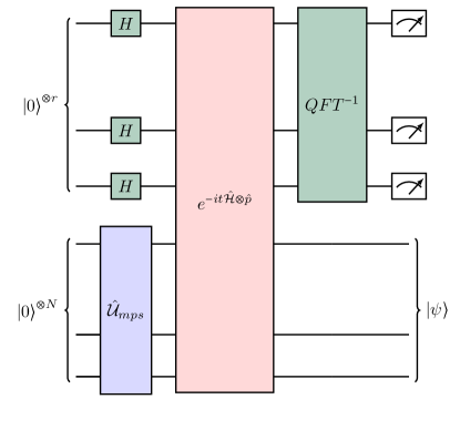
The von Neumann prescription provides a general framework for conducting measurements in quantum mechanics, applicable to all observables and systems. The procedure begins with initializing our quantum computer in the input state and introducing an ancillary subsystem, representing a continuous quantum degree of freedom such as a harmonic oscillator or a free particle on the line, initialized in the position “eigenstate” . This ancillary system acts as our meter, intended to gauge the energy of our quantum state. The position of the ancillary particle becomes correlated with the energy level of our state: the further to the right the particle is positioned, the higher the energy level. Upon performing a measurement on the ancillary subsystem, the state of the particle collapses to the eigenstate of the position observable corresponding to the measurement outcome [26, 27, 25, 24, 28].
We encounter a fundamental issue: the energy of a Hermitian operator can only be measured to a finite precision using a finite quantum circuit. Consequently, the depth of the quantum circuit required for this measurement scales with the desired accuracy, denoted by . This quantum circuit is constructed based on a discretization of von Neumann’s measurement prescription. It serves as a fundamental component in quantum algorithms, known, in one of its manifestations, as phase estimation [27, 29]. The schematic of the algorithm is depicted in Fig. 1.
We introduce an ancillary quantum variable, denoted as or a continuous pointer. To efficiently perform the above operation on a quantum computer, we discretize the pointer using qubits, replacing the continuous quantum variable with a -dimensional space. In this representation, the computational basis state of the pointer corresponds to the momentum eigenstates of the original continuous quantum variable, with the label representing the binary representation (bit-string encoding) of the integers from to . The discretized momentum operator becomes is defined as the sum of each , which individually acts on each ancillary qubit
| (2) |
such that the above normalization leads to
| (3) |
For example in the case of , there would be possible state .
If we initialize the pointer in a discretized state as a narrow wave packet centered at ,
| (4) |
This state can be efficiently prepared on a quantum computer by initializing the qubits of the pointer in the state and applying an (inverse) quantum Fourier transform. Since the momentum operator induces translational invariance, we can define a displacement operator by distance , which evolves of the state of Eq. 4 as follow
| (5) |
The main task here is to find out the specific eigenvalue of Hamiltonian .
The coupling between the Hamiltonian and the pointer is represented as , which for the Hamiltonian in Equation (1) is given as
| (6) |
By coupling the system to the pointers, one can define the operator , which acts on both system and pointer or ancillary qubits. When we allow the combined system and pointer to evolve for a time , the evolution is given by the equation
| (7) |
Here, represents an eigenstate of with eigenvalue , and we’ve set .
If we initialize the pointer in the state as Eq. 4, and the initial state of the system is , then the total state of the system+pointers would be , the discretized evolution in Eq. 7 simplifies to:
| (8) |
Which shifts the position of the pointer from to for each eigenstate of . Now, the discretized Hamiltonian is a sum of terms involving at most body-interaction, assuming represents a -body interaction system. Therefore, we can simulate the dynamics of using the method described above.
Now if the system is initially prepared in one of its eigenstate of the Hamiltonian, The discretized evolution of the system+pointer can be written
| (9) |
Performing an inverse quantum Fourier transform on the pointers leaves the system in the state , where:
| (10) |
Therefore, we find that
| (11) |
where
| (12) |
which is strongly peaked near . Here, corresponds to the eigenvalue associated with the eigenstate .
III.2 State preparation using DMRG algorithm
A key input for our approach is White’s Density Matrix Renormalization Group (DMRG) [6, 7, 5]. This is a classical numerical method to obtain a variational representation of the ground state in the form of what is known as a Matrix Product State (MPS), which is a state of the form [30, 31, 32, 7]:
| (13) |
where each is a rank- tensor. Note that the indices and range from to the bond dimension on site . The maximum value of the bond dimensions is denoted . We impose open boundary conditions by requiring that .
The DMRG is a class of numerical algorithms that proceeds by sequentially optimizing the variational degrees of freedom of an MPS, namely the rank-3 tensors . Abstractly, the DMRG works by carrying out the quadratic variational optimization
| (14) |
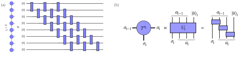
for each , and iterating until convergence is reached. It is now known that MPS provides a faithful representation for the ground state of gapped strongly correlated system [31, 32], ensuring the general applicability of the DMRG. Here we leverage the learnings gained in the application of the DMRG to quantum spin systems by exploiting a general quantum circuit construction to load an arbitrary MPS into a quantum register directly[33, 34, 35, 36, 37, 2, 38]. We summarise this construction here.
To describe how to load an MPS to its equivalent quantum circuit, we first ensure that the MPS is in right-canonical form[7, 39], by exploiting the gauge freedom of the MPS representation to enforce the additional conditions
| (15) |
The right-canonical condition ensures that each tensor is an isometry from to . Any isometry can be expressed as a unitary operation acting on an ancillary normalized state, denoted here as :
| (16) |
In this way we can realise a general MPS as a sequential staircase of -local unitary operators :
| (17) |
This construction is illustrated in Fig. 2. In this case, the maximum bond dimension satisfies ; The unitaries are 2-qubit gates. If then the unitaries necessarily act on more than qubits at a time. In this case, for implementation reasons, we must compile the unitaries in terms of local -qubit gates.
IV Applications
We consider two classes of strongly correlated systems to which our approach can be applied. quantum spin systems and electronic structure problems such as systems of molecules or nuclei.
IV.1 Quantum Spin Systems
We consider a system of interacting spins governed by the XXZ Hamiltonian in the form of the Heisenberg model, which has the following Hamiltonian
| (18) |
where is the coupling strength (here ) and , , are are the Pauli matrices acting nontrivially on spin and denotes the nearest-neighbor interaction between sites. To exemplify our results, we consider this model in a triangular lattice. Considering a triangular lattice (12 qubits) with periodic boundary conditions, Fig. 3 shows the results of the simulation of finding the ground state of such systems. Due to the effect of long-range correlations such as frustrations, Ground state simulation of these systems in higher dimensions larger than one is very challenging. By approximating the initial state as a DMRG state by the bond dimension , we can estimate the ground state close to the true ground state. Note that one can simulate a larger system, we choose such systems such that we know the exact ground state.
IV.2 Electronic structure problem
The definition of the first-quantized representation of the electronic Hamiltonian of a molecule consisting of electrons in atomic units reads as
| (19) |
where and are the position and charge of the nuclei, respectively, and denotes the position of the electrons. The electronic structure Hamiltonian has the following second-quantized form
| (20) |
where and are fermionic creation and annihilation operators associated with -th fermionic mode or spin-orbital and Where and are scaler coefficients and refer respectively to the one-body and two-body integrals. In the electron’s spatial and spin coordinates , the scalar coefficients in Eq. (20) are calculated from and [40, 41, 42, 43, 44, 45, 46, 47, 48, 49, 50, 51, 52, 53, 54, 55].
To implement the second-quantized form of the Hamiltonian on a quantum computer, we need to transform the fermionic Fock space to the qubit’s Hilbert space. This mapping makes the creation and annihilation operators of the fermions described by the unitary operators on the qubit. The three important methods for this mapping are Jordan-Wigner (JW), Bravyi-Kitaev (BK), and parity transformations[48, 56, 49, 51, 57].
In the actual simulations of molecules, the energy (molecular)correlations originated from three different sets of space orbitals: core orbitals, active orbitals, and external or virtual orbitals. Two electrons always occupy core orbitals. Active orbitals can be occupied by zero, one, or two electrons. The external orbitals are never occupied. Depending on the molecular structure and the task, one can proceed with how to simulate such systems. To demonstrate our method, Here we only consider the first a complete FCI including core orbitals and active orbitals. Active space selection is a way to reduce the number of qubits by ignoring some molecular orbitals in the post-Hartree-Fock calculation. Applying this method is trivial, but choosing which molecular orbitals to freeze is not. While there is no general algorithm to perform that operation, one can evaluate which orbitals to freeze by first printing the molecular orbital occupancy. One way of picturing this is only to consider frontier orbitals and their neighbors. The correlation lost on the total energy when only considering a subset of the full active space might be small. For example, freezing low-lying occupied molecular orbitals is known as the frozen-core approximation and can be applied because core orbitals do not mix with valence orbitals. Also, there are algorithms to freeze virtual orbitals, like the Frozen Natural Orbitals (FNO) truncation method. Another way of selecting active molecular orbitals is to consideration of molecular orbitals near the Highest occupied molecular orbital (HOMO) and Least unoccupied molecular orbital (LUMO) level. In this work, we consider two types of molecules: Octah-hydrogen with full orbitals and Pyridine with selecting only a set of active orbitals[42, 43, 44, 45, 46, 58].
To show how the algorithm works, We first start by expressing the reference state or Hartree-Fock state in terms of a simple product state and use it as an input for the DMRG algorithm. optimizing this state, we can have an initial solution with a specific bond dimension for the state as . In a practical simulation and for large-scale simulation, the is usually the maximum limit that a classical computer can reach. We expect to be an approximation to the ground state of the system, i.e., by increasing . In this work, in order to demonstrate the performance of the algorithm, we fix the bond dimension to a limited value.
IV.2.1 Full-configuration interaction (FCI) simulations with including frozen orbitals
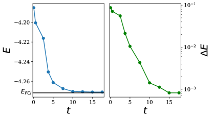
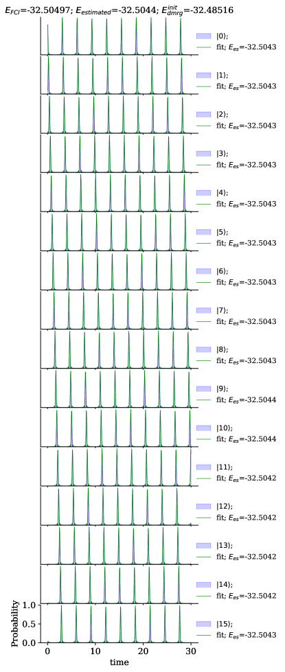
In this part, we present the results for FCI simulation without frozen orbitals. To show how the algorithm works, we choose an Octah-hydrogen molecule with FCI interaction energy with spatial orbitals and qubits with geometrical structure as shown is in the appendix B. We consider slater-type-orbitals with three primitive Gaussian orbitals sto-3g basis. To demonstrate how the algorithm works, we find an approximation for the ground state using the DMRG state with a small bond dimension, and then we feed this initial state to the quantum algorithm. In practice and in realistic situations, one deals with a large molecular system such that the DMRG method with a very large bond dimension would give only an approximation to the true ground state, and the rest can be carried on the quantum processor. In the Fig. 4. Fig. 5 shows the precision of the algorithm as a quantum circuit depth, which is represented by total time evolution. As time increases, the precision of the algorithm increases, and one can measure the ground state more accurately.
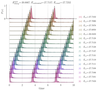
IV.2.2 Full-configuration interaction (FCI) simulations with selected active orbitals
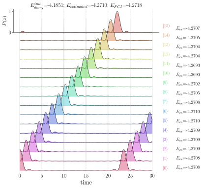
Pyridine is a type of protein that plays a critical role in DNA and RNA synthesis. It has a complex structure composed of amino acids. We select a set of active orbitals with HOMO and LUMO in the sto-3g basis. This allows us to reduce the quantum resources required from active orbitals and active electrons to active molecular orbitals and active electrons, meaning qubits. The results of the simulations are depicted in Fig. 6. Using the DMRG algorithm, We prepare the initial state as an approximation of the true full configuration ground state in terms of MPS with the bond dimension of and energy Hartree. By loading this initial state as the input to the algorithm, we are able to estimate the ground state of the system as , which is very close to and can be improved further. For the geometrical structure of the Pyridine, see the appendix B.

V Implementation
V.1 Suzuki-Trotter decomposition of time evolution operator
Expressing the Hamiltonian in the form of Eq. 1 or Eq. 6, we may then discretize the evolution operator using the first order Trotter-Suzuki approximation
| (21) |
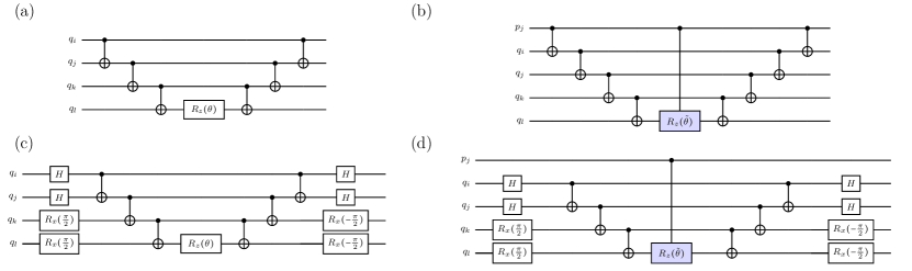
In the implementation of the quantum processor, one would usually need to implement the gates related to the time evolution operator. where , is the number of Trotter steps and is the Trotter time step. In a standard quantum circuit implementation, each is decomposed into single qubit rotations and CNOT gates. Fig. 7 shows two examples of such multiqubit gates.
V.2 Number of Gates
Here, we give an estimation of the amount of resources required for simulating molecules on a quantum device. As we have seen from section 20, specific Hamiltonian as in Eq. 1 has terms which any terms is a multi-qubit interaction. For a -local term in the Hamiltonian with interactions, we need CNOT gate with maximum one qubit gates as depicted in Fig. 7. Table 1 shows the total number of CNOT gates required for one time step in trotterized time evolution. There is also controlled- is required for each trotterized time step.
In many quantum computation applications, we usually have a pattern known as the conjugation pattern, and it is of form
| (22) |
then it is sufficient only to control the central operation. This means
| (23) |
Note that a controlled- can be written as
| (24) |
| Molecule | No. CNOT gates | No. of terms |
|---|---|---|
| 37500 | 2939 | |
| Pyridine() | 30444 | 2765 |
VI Tensor Networks Simulation
To illustrate the operation of the algorithm, our primary focus is on determining the ground state of a specific Hamiltonian denoted as . We employ the Density Matrix Renormalization Group (DMRG) technique to construct an initial state in the form of a Matrix Product State (MPS), with a designated bond dimension represented as . This MPS serves as an approximation of the ground state, denoted as . Subsequently, this state can be loaded into the corresponding quantum circuit on the quantum processor. To generate such an MPS state, it is imperative to represent the Hamiltonian, as expressed in Equation (1), as a Matrix Product Operator (MPO). Given that the Hamiltonian described in Equation (1) may entail long-range interactions, we utilize Matrix Product Diagrams [62, 63, 64] to identify the corresponding MPO for this Hamiltonian.
To benchmark and simulate the performance of the algorithm, we represent the Hamiltonians in the form of MPO and find an approximation for the ground state controlled by bond dimension using DMRG.
We start with MPO representation of the Hamiltonian
| (25) |
where each tensor is a matrix with being bond dimension at each bond between site and . and represent the local basis states at site i.
One can write the MPS form of the state as Eq. 13
| (26) |
We control the accuracy and size of tensor ’s with bond dimension .
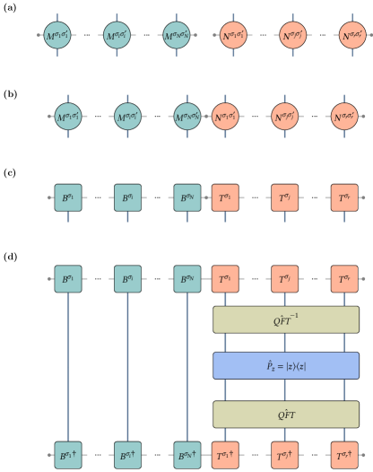
Fig. 8 (a) shows the corresponding MPO representation of the system and ancillary qubits before coupling to each other. We use open boundary conditions for both systems of ancillae, meaning that the bond dimension of MPO at the end of the chain is fixed to one. Fig. 8 (b) depicts the coupling between the system and pointers by attaching their MPO representation. The same analogy is applied for the MPS representation of the system+pointers coupling with open boundary condition as it is depicted in Fig. 8 (c).
For the time evolution of the composite system + pointer, we use the time-dependent variational principle (TDVP) algorithm[65, 66]. We time-evolve the system + pointer, and at specific time , one can measure the pointers in the computational basis by tracing out the system and application of quantum Fourier transformation as it is shown in the Fig. 8. In the practical implementation of the TDVP algorithm, we use two-site updates with varying bond dimensions during the time evolution. The maximum bond dimension used in the simulation is , and the time step for the time evolution is .
VI.1 Extension to excited states
Excited states can be, for instance, optimized sequentially with state-specific algorithms. After the optimization of the ground state , the first excited state is obtained from a constrained, variational optimization in the space orthogonal to the ground state.[67, 68, 63] This is achieved by replacing the Hamiltonian with its projected counterpart , defined as
| (27) |
In which is the ground state of the system. All terms appearing in Eq. (27) can be encoded as MPOs and therefore, the ground state of (i.e. the first excited state of ) can be optimized with the standard DMRG algorithm. Higher-lying excited states are then obtained from successive constrained optimizations.
VII Conclusion
In this work, we have demonstrated a hybrid approach combining classical methods with quantum algorithms to simulate complex quantum systems efficiently. Specifically, we utilized the Density Matrix Renormalization Group (DMRG) method for state preparation and combined it with a quantum algorithm based on von Neumann’s measurement prescription. This integration aims to enhance the precision and scalability of quantum simulations.
We have shown that tensor network methods, particularly DMRG, are powerful tools for preparing high-quality initial states for quantum algorithms. By representing the Hamiltonian and states as Matrix Product Operators (MPOs) and Matrix Product States (MPSs), respectively, we can leverage the strengths of classical computational techniques to handle large and complex quantum systems effectively.
Our algorithm was tested on various quantum systems, including strongly correlated spin systems and electronic structure problems of molecules like Octahydrogen () and Pyridine (). The results indicate that the hybrid approach not only provides a good approximation of the ground state but also allows for the precise measurement of energy levels through quantum circuits. Furthermore, we discussed the extension of this method to excited states, emphasizing the potential of variational approaches to improve the overall efficiency and accuracy of quantum simulations. This approach could be particularly useful in areas such as quantum chemistry and materials science, where accurate simulation of quantum systems is essential. Future directions for this research include exploring variational implementations of the algorithm[69, 70, 71].
VIII Acknowledgement
we would like to thank Tobias J. Osborne, Sören Wilkening for stimulating discussions. We acknowledge funding by the Ministry of Science and Culture of Lower Saxony through Quantum Valley Lower Saxony Q1 (QVLS-Q1)
References
- Cirac et al. [2021] J. I. Cirac, D. Pérez-García, N. Schuch, and F. Verstraete, Rev. Mod. Phys. 93, 045003 (2021).
- Astrakhantsev et al. [2023] N. Astrakhantsev, S.-H. Lin, F. Pollmann, and A. Smith, Phys. Rev. Res. 5, 033187 (2023).
- Bridgeman and Chubb [2017] J. C. Bridgeman and C. T. Chubb, Journal of Physics A: Mathematical and Theoretical 50, 223001 (2017).
- Biamonte and Bergholm [2017] J. Biamonte and V. Bergholm, Tensor networks in a nutshell (2017), arXiv:1708.00006 [quant-ph] .
- White [1992] S. R. White, Phys. Rev. Lett. 69, 2863 (1992).
- Schollwöck [2005] U. Schollwöck, Rev. Modern Phys. 77, 259 (2005).
- Schollwöck [2011] U. Schollwöck, Ann. Phys. 326, 96 (2011).
- Nielsen and Chuang [2010] M. A. Nielsen and I. L. Chuang, Quantum Computation and Quantum Information: 10th Anniversary Edition (Cambridge University Press, 2010).
- Portugal [2013] R. Portugal, Quantum Walks and Search Algorithms (Springer, New York, NY, 2013).
- Preskill [2018] J. Preskill, Quantum 2, 79 (2018), arxiv:1801.00862 .
- Peruzzo et al. [2014] A. Peruzzo, J. McClean, P. Shadbolt, M.-H. Yung, X.-Q. Zhou, P. J. Love, A. Aspuru-Guzik, and J. L. O’Brien, Nature Communications 5, 4213 (2014).
- Farhi et al. [2014] E. Farhi, J. Goldstone, and S. Gutmann, arXiv:1411.4028 [quant-ph] (2014), arXiv:1411.4028 [quant-ph] .
- Dborin et al. [2022a] J. Dborin, F. Barratt, V. Wimalaweera, L. Wright, and A. G. Green, Quantum Science and Technology 7, 035014 (2022a).
- Huang et al. [2022] J. Huang, W. He, Y. Zhang, Y. Wu, B. Wu, and X. Yuan, Tensor Network Assisted Variational Quantum Algorithm (2022), arXiv:2212.10421.
- Khan et al. [2023] A. Khan, B. K. Clark, and N. M. Tubman, 2310.12965 [cond-mat, physics:quant-ph] (2023).
- Shin et al. [2023] S. Shin, Y. S. Teo, and H. Jeong, 2307.06937 [quant-ph] (2023).
- Rieser et al. [2023] H.-M. Rieser, F. Köster, and A. P. Raulf, Proceedings of the Royal Society A: Mathematical, Physical and Engineering Sciences 479, 20230218 (2023), 2303.11735 [quant-ph] .
- Fan et al. [2023] Y. Fan, J. Liu, Z. Li, and J. Yang, 2301.06376 [physics, physics:quant-ph] (2023).
- Termanova et al. [2024] A. Termanova, A. Melnikov, E. Mamenchikov, N. Belokonev, S. Dolgov, A. Berezutskii, R. Ellerbrock, C. Mansell, and M. Perelshtein, Tensor quantum programming (2024), arXiv:2403.13486 [quant-ph] .
- Robledo-Moreno et al. [2024] J. Robledo-Moreno, M. Motta, H. Haas, A. Javadi-Abhari, P. Jurcevic, W. Kirby, S. Martiel, K. Sharma, S. Sharma, T. Shirakawa, I. Sitdikov, R.-Y. Sun, K. J. Sung, M. Takita, M. C. Tran, S. Yunoki, and A. Mezzacapo, Chemistry beyond exact solutions on a quantum-centric supercomputer (2024), arXiv:2405.05068 [quant-ph] .
- Kitaev [1995] A. Y. Kitaev, Electron. Colloquium Comput. Complex. TR96 (1995).
- Abrams and Lloyd [1999] D. S. Abrams and S. Lloyd, Phys. Rev. Lett. 83, 5162 (1999).
- Mohammadbagherpoor et al. [2019] H. Mohammadbagherpoor, Y.-H. Oh, P. Dreher, A. Singh, X. Yu, and A. J. Rindos, An improved implementation approach for quantum phase estimation on quantum computers (2019), arXiv:1910.11696 [quant-ph] .
- Novo et al. [2021] L. Novo, J. Bermejo-Vega, and R. García-Patrón, Quantum 5, 465 (2021).
- Childs et al. [2002] A. M. Childs, E. Deotto, E. Farhi, J. Goldstone, S. Gutmann, and A. J. Landahl, Phys. Rev. A 66, 032314 (2002).
- [26] J. von Neumann, Mathematical Foundations of Quantum Mechanics, Princeton University Press.
- Mello [2014] P. A. Mello, AIP Conference Proceedings 1575, 136 (2014).
- Vermersch et al. [2019] B. Vermersch, A. Elben, L. M. Sieberer, N. Y. Yao, and P. Zoller, Phys. Rev. X 9, 021061 (2019).
- Temme et al. [2011] K. Temme, T. J. Osborne, K. G. Vollbrecht, D. Poulin, and F. Verstraete, Nature 471, 87 (2011).
- Fannes et al. [1994] M. Fannes, B. Nachtergaele, and R. F. Werner, Journal of Functional Analysis 120, 511 (1994).
- Verstraete and Cirac [2006] F. Verstraete and J. I. Cirac, prb 73, 094423 (2006).
- Hastings [2007] M. B. Hastings, J. Stat. Mech. , P08024 (2007).
- Schoen et al. [2007] C. Schoen, K. Hammerer, M. M. Wolf, J. I. Cirac, and E. Solano, Phys. Rev. A 75, 032311 (2007), quant-ph/0612101 .
- Ran [2020] S.-J. Ran, Phys. Rev. A 101, 032310 (2020).
- Lin et al. [2021] S.-H. Lin, R. Dilip, A. G. Green, A. Smith, and F. Pollmann, PRX Quantum 2, 010342 (2021).
- Rudolph et al. [2022] M. S. Rudolph, J. Chen, J. Miller, A. Acharya, and A. Perdomo-Ortiz, Decomposition of matrix product states into shallow quantum circuits (2022), arXiv:2209.00595 [quant-ph] .
- Dborin et al. [2022b] J. Dborin, F. Barratt, V. Wimalaweera, L. Wright, and A. G. Green, Quantum Science and Technology 7, 035014 (2022b).
- Javanmard et al. [2024] Y. Javanmard, U. Liaubaite, T. J. Osborne, X. Xu, and M.-H. Yung 10.48550/arXiv.2401.02355 (2024), arXiv:2401.02355 [cond-mat, physics:quant-ph].
- Javanmard et al. [2018] Y. Javanmard, D. Trapin, S. Bera, J. H. Bardarson, and M. Heyl, New Journal of Physics 20, 083032 (2018).
- Bauer et al. [2020] B. Bauer, S. Bravyi, M. Motta, and G. K.-L. Chan, Chemical Reviews 120, 12685 (2020).
- Head-Marsden et al. [2021] K. Head-Marsden, J. Flick, C. J. Ciccarino, and P. Narang, Chemical Reviews 121, 3061 (2021).
- Senicourt et al. [2022] V. Senicourt, J. Brown, A. Fleury, R. Day, E. Lloyd, M. P. Coons, K. Bieniasz, L. Huntington, A. J. Garza, S. Matsuura, R. Plesch, T. Yamazaki, and A. Zaribafiyan 10.48550/arXiv.2206.12424 (2022), arXiv:2206.12424 .
- Sun et al. [2017] Q. Sun, T. C. Berkelbach, N. S. Blunt, G. H. Booth, S. Guo, Z. Li, J. Liu, J. McClain, E. R. Sayfutyarova, S. Sharma, S. Wouters, and G. K.-L. Chan, arXiv preprint arXiv:1701.08223 (2017).
- McQuarrie [2016] D. A. McQuarrie, Quantum Chemistry (Viva Books, Neu Dehli, 2016).
- Engel [2009] T. Engel, Quantum Chemistry & Spectroscopy: International Edition, 2nd ed. (Pearson, Boston, Mass., 2009).
- Szabo and Ostlund [1996] A. Szabo and N. S. Ostlund, Modern Quantum Chemistry: Introduction to Advanced Electronic Structure Theory, revised ed. edition ed. (Dover Publications Inc., Mineola, New York, 1996).
- Sajjan et al. [2022] M. Sajjan, J. Li, R. Selvarajan, S. Hari Sureshbabu, S. Suresh Kale, R. Gupta, V. Singh, and S. Kais, Chemical Society Reviews 51, 6475 (2022).
- McArdle et al. [2020] S. McArdle, S. Endo, A. Aspuru-Guzik, S. C. Benjamin, and X. Yuan, Rev. Mod. Phys. 92, 015003 (2020).
- Cao et al. [2019] Y. Cao, J. Romero, J. P. Olson, M. Degroote, P. D. Johnson, M. Kieferová, I. D. Kivlichan, T. Menke, B. Peropadre, N. P. D. Sawaya, S. Sim, L. Veis, and A. Aspuru-Guzik, Chemical Reviews 119, 10856 (2019).
- Lanyon et al. [2010] B. P. Lanyon, J. D. Whitfield, G. G. Gillett, M. E. Goggin, M. P. Almeida, I. Kassal, J. D. Biamonte, M. Mohseni, B. J. Powell, M. Barbieri, A. Aspuru-Guzik, and A. G. White, Nature Chemistry 2, 106 (2010).
- Whitfield et al. [2011] J. D. Whitfield, J. Biamonte, and A. Aspuru-Guzik, Molecular Physics (2011), publisher: Taylor & Francis Group.
- O’Malley et al. [2016] P. J. J. O’Malley, R. Babbush, I. D. Kivlichan, J. Romero, J. R. McClean, R. Barends, J. Kelly, P. Roushan, A. Tranter, N. Ding, B. Campbell, Y. Chen, Z. Chen, B. Chiaro, A. Dunsworth, A. G. Fowler, E. Jeffrey, E. Lucero, A. Megrant, J. Y. Mutus, M. Neeley, C. Neill, C. Quintana, D. Sank, A. Vainsencher, J. Wenner, T. C. White, P. V. Coveney, P. J. Love, H. Neven, A. Aspuru-Guzik, and J. M. Martinis, Phys. Rev. X 6, 031007 (2016).
- Collaborators*† et al. [2020] G. A. Q. Collaborators*†, , F. Arute, K. Arya, R. Babbush, D. Bacon, J. C. Bardin, R. Barends, S. Boixo, M. Broughton, B. B. Buckley, D. A. Buell, B. Burkett, N. Bushnell, Y. Chen, Z. Chen, B. Chiaro, R. Collins, W. Courtney, S. Demura, A. Dunsworth, E. Farhi, A. Fowler, B. Foxen, C. Gidney, M. Giustina, R. Graff, S. Habegger, M. P. Harrigan, A. Ho, S. Hong, T. Huang, W. J. Huggins, L. Ioffe, S. V. Isakov, E. Jeffrey, Z. Jiang, C. Jones, D. Kafri, K. Kechedzhi, J. Kelly, S. Kim, P. V. Klimov, A. Korotkov, F. Kostritsa, D. Landhuis, P. Laptev, M. Lindmark, E. Lucero, O. Martin, J. M. Martinis, J. R. McClean, M. McEwen, A. Megrant, X. Mi, M. Mohseni, W. Mruczkiewicz, J. Mutus, O. Naaman, M. Neeley, C. Neill, H. Neven, M. Y. Niu, T. E. O’Brien, E. Ostby, A. Petukhov, H. Putterman, C. Quintana, P. Roushan, N. C. Rubin, D. Sank, K. J. Satzinger, V. Smelyanskiy, D. Strain, K. J. Sung, M. Szalay, T. Y. Takeshita, A. Vainsencher, T. White, N. Wiebe, Z. J. Yao, P. Yeh, and A. Zalcman, Science 10.1126/science.abb9811 (2020).
- Hempel et al. [2018] C. Hempel, C. Maier, J. Romero, J. McClean, T. Monz, H. Shen, P. Jurcevic, B. P. Lanyon, P. Love, R. Babbush, A. Aspuru-Guzik, R. Blatt, and C. F. Roos, Phys. Rev. X 8, 031022 (2018).
- McClean et al. [2017] J. R. McClean, M. E. Kimchi-Schwartz, J. Carter, and W. A. de Jong, Phys. Rev. A 95, 042308 (2017).
- Jordan and Wigner [1928] P. Jordan and E. Wigner, Zeitschrift für Physik 47, 631 (1928).
- Seeley et al. [2012] J. T. Seeley, M. J. Richard, and P. J. Love, The Journal of Chemical Physics 137, 224109 (2012).
- Verma et al. [2021] P. Verma, L. Huntington, M. P. Coons, Y. Kawashima, T. Yamazaki, and A. Zaribafiyan, The Journal of Chemical Physics 155, 034110 (2021).
- Cowtan et al. [2020] A. Cowtan, S. Dilkes, R. Duncan, W. Simmons, and S. Sivarajah, Electronic Proceedings in Theoretical Computer Science 318, 213–228 (2020).
- Sivarajah et al. [2020] S. Sivarajah, S. Dilkes, A. Cowtan, W. Simmons, A. Edgington, and R. Duncan, Quantum Science and Technology 6, 014003 (2020).
- Peng et al. [2022] B. Peng, S. Gulania, Y. Alexeev, and N. Govind, Physical Review A 106, 012412 (2022).
- Crosswhite and Bacon [2008] G. M. Crosswhite and D. Bacon, Phys. Rev. A 78, 012356 (2008).
- Keller et al. [2015] S. Keller, M. Dolfi, M. Troyer, and M. Reiher, The Journal of Chemical Physics 143, 244118 (2015).
- Ren et al. [2020] J. Ren, W. Li, T. Jiang, and Z. Shuai, The Journal of Chemical Physics 153, 084118 (2020).
- Haegeman et al. [2011] J. Haegeman, J. I. Cirac, T. J. Osborne, I. Pižorn, H. Verschelde, and F. Verstraete, Physical Review Letters 107, 070601 (2011).
- Haegeman et al. [2016] J. Haegeman, C. Lubich, I. Oseledets, B. Vandereycken, and F. Verstraete, Physical Review B 94, 165116 (2016).
- Baiardi and Reiher [2020] A. Baiardi and M. Reiher, The Journal of Chemical Physics 152, 040903 (2020).
- McCulloch [2007] I. P. McCulloch, Journal of Statistical Mechanics: Theory and Experiment 2007, P10014 (2007).
- Filip et al. [2024] M.-A. Filip, D. M. Ramo, and N. Fitzpatrick, Quantum 8, 1278 (2024).
- Liu et al. [2023] C.-Y. Liu, C.-H. A. Lin, and K.-C. Chen, Learning quantum phase estimation by variational quantum circuits (2023), arXiv:2311.04690 [quant-ph] .
- Cîrstoiu et al. [2020] C. Cîrstoiu, Z. Holmes, J. Iosue, L. Cincio, P. J. Coles, and A. Sornborger, npj Quantum Information 6, 82 (2020).
Appendix A Jordan-Wigner Transformation
The Jordan-Wigner transformation maps fermions onto ordered qubits by assigning to the value of the th qubit the occupation of the th fermionic mode and stores the parity information on the occupation of the modes providing the index with a check on the corresponding qubits. It is defined as a correspondence between fermionic creation and annihilation operators and qubit operators
| (28) |
Where and fermionic creation and annihilation operators and satisfy the canonical anti-commutation relations
Appendix B Molecular geometry used in this work
Below is the geometrical structure of the Octah-hydrogen and Pyridine used in this work. The geometrical structure of reads as
| x | y | z | |
| H | 1.6180339887, | 0. | 0. |
| H | 1.3090169944, | 0.9510565163 | 0. |
| H | 0.5, | 1.5388417686 | 0. |
| H | -0.5, | 1.5388417686 | 0. |
| H | -1.3090169944, | 0.9510565163 | 0. |
| H | -1.6180339887, | 0. | 0. |
| H | -1.3090169944, | -0.9510565163 | 0. |
| H | -0.5, | -1.5388417686 | 0. |
and the geometrical structure of Pyridine reads as
| x | y | z | |
| C | 1.3603, | 0.0256, | 0. |
| C | 0.6971, | -1.2020, | 0. |
| C | -0.6944, | -1.2184, | 0. |
| C | -1.3895 | -0.0129, | 0. |
| C | -0.6712, | 1.1834, | 0. |
| N | 0.6816, | 1.1960, | 0. |
| H | 2.4530, | 0.1083, | 0. |
| H | 1.2665, | -2.1365, | 0. |
| H, | -1.2365, | -2.1696, | 0. |
| H, | -2.4837, | 0.0011, | 0. |
| H, | -1.1569, | 2.1657, | 0. |
Appendix C Another Example
Fig. 9 is the result for the simulation of molecule in the stog6 basis with following geometrical coordinate
| x | y | z | |
| B | 0., | 0., | 0. |
| H | 0., | 1., | 1. |
| H | 1., | 1., | 0. |