Bayesian Mapping of Mortality Clusters

Abstract

Disease mapping analyses the distribution of several disease outcomes within a territory. Primary goals include identifying areas with unexpected changes in mortality rates, studying the relation among multiple diseases, and dividing the analysed territory into clusters based on the observed levels of disease incidence or mortality. In this work, we focus on detecting spatial mortality clusters, that occur when neighbouring areas within a territory exhibit similar mortality levels due to one or more diseases. When multiple causes of death are examined together, it is relevant to identify not only the spatial boundaries of the clusters but also the diseases that lead to their formation. However, existing methods in literature struggle to address this dual problem effectively and simultaneously. To overcome these limitations, we introduce perla, a multivariate Bayesian model that clusters areas in a territory according to the observed mortality rates of multiple causes of death, also exploiting the information of external covariates. Our model incorporates the spatial structure of data directly into the clustering probabilities by leveraging the stick-breaking formulation of the multinomial distribution. Additionally, it exploits suitable global-local shrinkage priors to ensure that the detection of clusters is driven by concrete differences across mortality levels while excluding spurious differences. We propose an MCMC algorithm for posterior inference that consists of closed-form Gibbs sampling moves for nearly every model parameter, without requiring complex tuning operations. This work is primarily motivated by a case study on the territory of a local unit within the Italian public healthcare system, known as ULSS6 Euganea. To demonstrate the flexibility and effectiveness of our methodology, we also validate perla with a series of simulation experiments and an extensive case study on mortality levels in U.S. counties.
Keywords: Multinomial stick-breaking; Global-local shrinkage priors; Multivariate areal data clustering; Spatial disease mapping

1 Introduction

1.1 Motivation and case studies

In the analysis of environmental and epidemiological phenomena, researchers often gather geolocalised data in the form of multiple outcomes. For example, studies on the effects of long-term exposure to air pollution and high temperatures on public health generally collect and analyse both multiple environmental indicators and multiple health indicators (Künzli et al., 2000, Wong et al., 2008, Lee et al., 2009, Taylor et al., 2015). In epidemiological studies, multiple outcomes are used to determine the frailty characteristics of specific populations of patients (Li et al., 2021, Qian et al., 2023). Therefore, analysing the joint distribution of multiple outcomes and their interactions is a crucial step to uncover patterns in space and relationships that may not be evident when analysing each outcome on its own. This process provides a more comprehensive understanding of the underlying processes.

Disease mapping, in particular, aims at studying the spatial distribution of health phenomena to identify significant changes of diseases incidence or mortality. It therefore represents the first step for understanding geographical disparities in health outcomes and developing strategies for disease prevention and control. Disease mapping techniques have evolved significantly over the last decades, moving from simple representations of a disease occurrence to more advanced statistical analyses and models (Waller and Gotway, 2004, Lawson, 2013, Banerjee et al., 2015). The use of advanced statistical models yield a more detailed representation of the spatial distribution of phenomena in space and of the dependence across outcomes, resulting in more accurate explanatory and predictive performances (Aungkulanon et al., 2017, Coker et al., 2023, Griffith, 2023, Tesema et al., 2023). One of the main goals of disease mapping is discovering and locating clusters in space. A spatial cluster consists of a group of spatially proximate areas that show similar levels of the outcomes considered. In public health, discovering spatial clusters of disease incidence or mortality is crucial, as it represents a step forward in the identification of possible underlying risk factors in specific areas of the territory (Kulldorff, 1997, Kulldorff et al., 2005, Robertson et al., 2010).

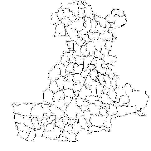
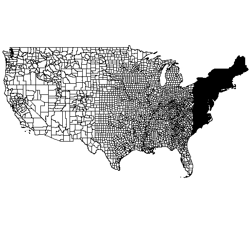
Figure 1: Left: map of the Padua province territory, which covers about 2,144 km² with a population of approximately 936,000 residents and a uniformly high population density (436 pop./km²). Right: map of the U.S. divided into counties. We highlighted the 388 counties on the U.S. East coast that we analysed in Section 5.2. Maps are not shown on the same scale.

For instance, we consider a study of mortality levels in the Padua province, located in northeastern Italy, with data provided by the local healthcare unit ULSS6 Euganea. ULSS6 oversees health services across the Padua province, whose territory is divided into 106 administrative sub-areas (the city of Padua is not considered as a stand-alone municipality but is divided into six districts of size and population comparable to other municipalities in the province). The goal of ULSS6 is to optimise logistical and financial resources by identifying significant variations in mortality levels across either individual areas or clusters of areas. Their interest is particularly focused on the mortality due to three major death causes: diseases of the circulatory system, diseases of the respiratory system, and malignant neoplasm. According to Fedeli et al. (2021), these three categories collectively represent 70% of the overall mortality rate recorded in the province. Mortality data for these death causes are available from 2017 to 2019, divided by gender. The left panel of Figure 1 illustrates the distribution of the 106 districts managed by ULSS6 across the province territory. The left panel of Supplementary Figure 1 displays the geographical position of the Padua province in Italy. Bovo et al. (2023) made a first attempt to detect mortality clusters in this province by analysing each cause of death separately. Nonetheless, we recognise some important limitations in this approach since treating the variables independently can lead to identify clusters that vary substantially for each cause of death. Moreover, this method does not take full advantage of the information across variables, meaning the clustering of the territory driven by one cause of death lacks insight from the data of other causes. In contrast, gaining information from all causes of death simultaneously would lead to the identification of territorial clusters with specific mortality profiles, i.e., with distinct risk levels for each cause of death.

The case study of ULSS6 mortality data is relevant due to its depiction of a setting where areas have similar territorial characteristics, comparable population sizes and socio-economic conditions. On the other hand, in many other cases, the territory under consideration may be highly heterogeneous in one or more aspects. For instance, in the United States of America (U.S.) the administrative division of the territory into counties provides a far different scenario from the province of Padua. The distribution of population in space is heterogeneous, as well as population density, urbanisation and wealth; in addition, different U.S. states may have different health care systems, and this leads to another source of variability. The distribution of U.S. counties in space is displayed in the right panel of Figure 1. In this framework, the Centres for Disease Control and Prevention (CDC) collected data on mortality levels by counties in the U.S. from 2016 to 2019, available through the WONDER Online Databases (CDC, 2021). In such diverse contexts, it is crucial not only to quantify different risk levels across areas, but also to determine the existence of possible geographically concentrated clusters with specific epidemiological relevance.

Both the discussed examples reveal the need for a statistical method that can: i.) perform multivariate clustering of a territory based on the joint analyses of multiple outcomes, exploiting the spatial structure of data and the dependence across diseases; ii.) leverage information provided by exogenous variables that influence the outcomes; and iii.) identify which of the outcome variables lead to the formation of spatial clusters. This last point becomes more and more relevant as the number of outcomes increases or the size of the territory grows, making it essential to identify clusters of disease prevalence or excess mortality that are geographically concentrated in small areas while avoiding spurious signals.

1.2 Spatial clustering of mortality levels

In this article, we consider the problem of clustering areas of a territory based on the observed outcomes of multiple diseases. We assume that the territory is divided into polygons defined by administrative boundaries, and that the outcome variables are aggregates of measures taken within the boundaries of each area. In the ULSS6 Euganea case study presented in Section 1.1, the areas correspond to municipalities or administrative districts, while in the U.S. dataset the areas represent the U.S. counties. In both studies, the outcome variables are measurements of mortality from multiple causes of death.

A common approach for identifying groups of contiguous areas with excess of mortality, and thus detecting some spatial clusters, is through spatial scan statistics (SSS, Kulldorff, 1997). These techniques are designed to detect clusters with unexpected changes in outcome variable levels compared to the rest of the territory. This detection is carried out using suitable test statistics (Ahmed and Genin, 2020, Cucala, 2016, Liu et al., 2018). Over the past twenty years, these techniques have gained considerable attention and have been adapted for spatio-temporal data analysis in both frequentist (Kulldorff et al., 2005, Robertson et al., 2010, Amini et al., 2023) and Bayesian paradigms (Li et al., 2012). Recently, SSS have been largely extended also to the multivariate framework (Cucala et al., 2017, 2019) and to more complex data structures, such as multivariate functional data (Frévent et al., 2023). For a detailed review of applications of multivariate SSS to different contexts, readers can refer to the Introduction section of Frévent et al. (2023). Despite their extensive use, SSS are primarily designed to detect abrupt changes in outcome variables and thus they cannot be used to divide the entire map into clusters. In addition, SSS may fail to detect significant changes in areas with highly irregular shapes (Tango, 2021).

Another established approach for detecting spatial clusters is through hidden Potts models (HPM), introduced as an extension of the Gaussian mixture models (GMM) to account for spatial dependence across adjacent neighbours (Potts, 1952). In Bayesian literature, inference on HPM has been extensively explored using various approaches. Examples include Markov chain Monte Carlo (MCMC) methods (Green and Richardson, 2002), variational Bayes (McGrory et al., 2009), and approximate Bayesian computation (Moores et al., 2020a). Recent advancements also include estimation based on synthetic likelihood (Zhu and Fan, 2023). For a comprehensive review of HPM estimation methods, readers can refer to Moores et al. (2020b). Despite their popularity, the Potts model presents some relevant drawbacks, particularly related to the estimation of the inverse temperature parameter. Recently, Moores et al. (2020a) made a detailed survey of the approaches investigated so far for bypassing the estimation problems of HPM, with particular attention to Approximate Bayesian Computation algorithms, and proposed their own scalable solution. However, the current statistical literature does not adequately address the extension of HPM to the joint analysis of multiple outcomes. Additionally, to the best of our knowledge, there is no implementation of a multivariate Potts model available, for instance, for the R programming language (R Core Team, 2024).

To address the need to identify mortality clusters jointly considering multiple causes of death, we propose perla (PEnalised Regression with Localities Aggregation), a multivariate Bayesian model for areal data that aggregates areas of a territory into spatially informed clusters based on different levels of outcome variables, while accounting for the presence of exogenous variables and for the marginal correlation across responses. Recently, Coker et al. (2023) applied a Dirichlet process mixture model to the analysis of areal data, without accounting for the spatial structure in the clustering phase. Instead, perla integrates the data spatial proximity directly into the clustering probabilities using the multinomial stick-breaking strategy of Linderman et al. (2015). This method consists of rewriting a multinomial model as a sequence of binomial random variables, allowing the use of the well-established Pólya-gamma data augmentation in the presence of multinomial outcomes. Not only does the multinomial stick-breaking consent the Bayesian inference to be performed in closed form, but it also allows avoiding the use of the Potts model to account for the neighbourhood structure and consequently avoiding the known inferential problems associated with it. Alternative approaches to link a probability vector defined on a simplex to a series of Gaussian random variables include, for example, the logistic normal distribution (Lafferty and Blei, 2005, Russo et al., 2022). In addition, perla regulates the clusters intercepts through global-local shrinkage priors (Polson and Scott, 2011), allowing to affirm or inhibit the role of specific diseases in the formation of clusters.The shrinkage priors play also a regularising role in the selection of the number of clusters, as they help suppressing the effect of excess clusters. The reader can refer to Bhadra et al. (2019) and van Erp et al. (2019) for two reviews of global-local shrinkage priors.

This work is strongly motivated by the two epidemiological case studies presented in Section 1.1 and can be of great usefulness in the analysis of several other social and epidemiological phenomena, including the distribution of the level of education, the incidence of diseases, and the occurrence of multiple kind of crimes. Nonetheless, perla can be applied to any kind of multivariate areal data. Two examples of the numerous possible applications outside the epidemiological context are image segmentation (Moores et al., 2015) and spatial transcriptomics (Zhao et al., 2021). For these reasons, we implemented our methodological solution in the software library perla for the R programming language.

The remainder of this article is structured as follows. Section 2 introduces the perla model, highlighting the formulation of the prior distributions and their role in the detection of spatial clusters. Section 3 delineates a MCMC algorithm to perform posterior inference, and explains how to operate model selection and post-processing using the posterior samples. Section 4 presents two simulation experiments. The goal of the first experiment is to demonstrate the significant improvements in clustering results and inferential conclusions provided by our global-local shrinkage priors compared to standard, non-informative priors. In addition, it performs a comparison of the clustering accuracy with other competing methods. The second experiment investigates whether different a priori choices on model parameters that handle the spatial correlation of the clustering probabilities have an impact on the final clustering performance, in particular when spatial clusters present different levels of spatial association. Section 5 presents the application of perla on the two cases studies described in Section 1.1, showing the usefulness of our methodology in responding to specific epidemiological questions. Finally, Section 6 takes some concluding remarks and outlines future perspectives.

2 Model formulation

2.1 The statistical model

We assume that data are collected in the form of an $n\times d$ matrix $\mathbf{Y}$, where $y_{ij}\in\mathbb{R}$ denotes the mortality level due to the $j$-th disease ($j=1,\dots,d$) measured at the $i$-th area of a map ($i=1,\dots,n$). Data are structured such that $y_{ij}>0$ denotes a mortality excess, and $y_{ij}<0$ denotes a mortality deficit. In addition, let $\mathbf{X}$ be an $n\times p$ matrix collecting $p$ exogenous variables whose values are available for the $n$ areas. We assume that the $n$ areas can be divided into $K$ territorial clusters, implying that the average mortality levels in the $i$-th spatial area due to the $d$ diseases considered vary based on the cluster to which the $i$-th area belong. We collect the information about the unknown clusters into a $n\times K$ matrix $\mathbf{Z}$, where $\mathrm{Z}_{ik}=1$ if the $i$-th area belongs to the $k$-th cluster (with $k=1,\dots,K$), and 0 otherwise. To access the rows and the columns of a generic matrix of parameters $\boldsymbol{\theta}$, we use the notation $\boldsymbol{\theta}_{i.}$ and $\boldsymbol{\theta}_{.j}$ to refer to its $i$-th row and its $j$-th column, respectively. The same notation is used also for the data matrices $\mathbf{Y}$ and $\mathbf{X}$, with the only exception that their row and column vectors are denoted with bold lowercase letters.

We assume that regions within a spatial cluster have similar mortality levels for each disease considered, whereas significant variations in mortality levels occur across clusters. In addition, we assume that exogenous variables influence the outcomes but do not regulate the formation of clusters (Coker et al., 2023). Based on these considerations, we formulate the multivariate regression model

$$\mathbf{y}_{i.}=\mathbf{Z}^{T}_{i.}\boldsymbol{\mu}+\mathbf{x}^{T}_{i.}\boldsymbol{\beta}+\boldsymbol{\epsilon}_{i.},\hskip 28.45274pt\boldsymbol{\epsilon}_{i.}|\boldsymbol{\Sigma}\sim\mathcal{N}_{d}(\mathbf{0},\boldsymbol{\Sigma}),$$ (1)

where $\mathbf{Z}_{i.}$ and $\mathbf{x}_{i.}$ are the $i$-th row of $\mathbf{Z}$ and $\mathbf{X}$, $\boldsymbol{\mu}=\{\mu_{kj}\}_{k=1,\dots,K,j=1,\dots,d}$ is a matrix containing the cluster- and disease-specific intercepts, $\boldsymbol{\beta}=\{\beta_{\ell j}\}_{\ell=1,\dots,p,j=1,\dots,d}$ is the matrix of regression coefficients, and $\boldsymbol{\epsilon}_{i.}$ is the vector of error terms. $\boldsymbol{\Sigma}$ aims at capturing the correlation across the $d$ diseases. The formulation of the regression model in (1) is equivalent to assuming a matrix variate Gaussian distribution on the outcome matrix $\mathbf{Y}$, with mean matrix $\mathbf{Z\boldsymbol{\mu}}+\mathbf{X\boldsymbol{\beta}}$, $\mathbb{I}_{n}$ as covariance matrix of the rows, and $\boldsymbol{\Sigma}$ as covariance matrix of the columns.

By definition of $\mathbf{Z}$, we define a cluster as a set of labelled areas with the same average levels of the $d$ responses, net of the effects of the covariates $\mathbf{X}$. Since the clustering matrix $\mathbf{Z}$ is unknown, we assume that $\mathbf{Z}_{i.}$ distributes according to a multinomial distribution of size 1 and vector of probabilities $\boldsymbol{\pi}_{i}=(\pi_{i1},\dots,\pi_{iK})$. To let the clustering draw information by the spatial structure of data, we first express the multinomial model as a series of binomial probability functions using the multinomial stick-breaking representation of Linderman et al. (2015)

$$\Pr(\mathbf{Z}_{i.}|\tilde{\boldsymbol{\pi}}_{i})=\prod_{k=1}^{K-1}\left\{\tilde{\pi}_{ik}^{\mathrm{Z}_{ik}}(1-\tilde{\pi}_{ik})^{1-\mathrm{Z}_{ik}}\right\}^{N_{ik}},$$ (2)

where $N_{i1}=1$ (there is at most one element per row that is equal to one), $\tilde{\pi}_{i1}={\pi}_{i1}$, and, for $k>1$,

$$\hskip 19.91684ptN_{ik}=1-\sum_{k^{\prime}<k}\mathrm{Z}_{ik^{\prime}},\hskip 14.22636pt\tilde{\pi}_{ik}=\dfrac{\pi_{ik}}{1-\sum_{k^{\prime}<k}\pi_{ik^{\prime}}}.$$

By construction, $\tilde{\pi}_{iK}=1$. Then, for $k=1,\dots,K-1$, we reparametrise the probabilities $\tilde{\pi}_{ik}$ using the logistic function, thus writing $\tilde{\pi}_{ik}=\exp(\psi_{ik})/\{1+\exp(\psi_{ik})\}$. The vector $\boldsymbol{\psi}_{.k}=(\psi_{1k},\dots,\psi_{nk})$ contains $n$ realisations in space of the transformed conditional probabilities of belonging to cluster $k$, given that the observations were not assigned to the previous $k-1$ clusters $(\boldsymbol{\psi}_{.1}$ simply represents the transformed probabilities of belonging to cluster 1). To introduce spatial dependence across the transformed clustering probabilities, we assume that each vector $\boldsymbol{\psi}_{.k}$ distributes according to a conditionally autoregressive (CAR) model of the form

$$\boldsymbol{\psi}_{.k}|\tau_{k},\rho_{k}\sim\mathcal{N}_{n}\{\boldsymbol{0},\tau_{k}(\mathbf{D}-\rho_{k}\mathbf{W})^{-1}\},$$ (3)

where $\mathbf{W}$ has null diagonal and $\mathrm{W}_{ii^{\prime}}=1$ if regions $i$ and $i^{\prime}$ are neighbours, and 0 otherwise, $\mathbf{D}$ is a diagonal matrix with $\mathrm{D}_{ii}$ equal to the number of neighbours of $i$, $\tau_{k}>0$ and $\rho_{k}\in[0,1]$.

Although the model in (3) does not force the areas within the same cluster to be connected by a path, therefore allowing even spatially distant areas to belong to the same cluster, modelling the clustering probabilities with CAR distributions as in (3) encourage the identification of spatially separated clusters. The principal role of $\rho_{k}$ is ensuring that $\mathbf{D}-\rho_{k}\mathbf{W}$ is positive definite. As discussed in Section 4.3.1 of Banerjee et al. (2015), $\rho_{k}$ cannot be interpreted as a measure of spatial correlation of data, similarly for example to what is expressed by Moran’s I. The only exception is $\rho_{k}=0$, which denotes the case of independence across spatial areas. To solve these oddities, Datta et al. (2019) proposed an alternative to the CAR formulation, named DAGAR, using a directed acyclic graph (DAG) to model the precision matrix of $\boldsymbol{\psi}_{.k}$. One of the key advantages of their approach lies in the interpretation of $\rho_{k}$, which now represents the degree of spatial correlation within the data. However, for this study, we have opted to retain the CAR formulation for mainly two reasons. Firstly, the DAGAR model necessitates the ordering of map areas. While Datta et al. (2019) demonstrate that ordering does not heavily impact the final results, it is not clear how the ordering operation should be performed when the statistical units, i.e., the spatial areas, are divided into clusters. In addition, the concept of ordering spatial data may pose challenges for non-experts in the field. Given our intention for the model to be used in epidemiological studies, we prefer to maintain a standard framework that does not rely on ordering. Secondly, our decision is reinforced by the favourable performance of the CAR model compared to DAGAR, as evidenced by Datta et al. (2019). Their study indicates that both models yield comparable results from various perspectives, with the interpretability of $\rho_{k}$ emerging as the primary advantage of DAGAR over CAR. In our application, we employ the spatial model solely to incorporate spatial correlation into the parameterised clustering probabilities $\boldsymbol{\psi}_{.k}$. Thus, we are not using a spatial model for the raw data itself, but rather for a latent parameter. Therefore, while interpretable, we believe that $\rho_{k}$ would offer a few epidemiological insights.

With the current formulation and assumptions, the stick-breaking construction offers a natural ordering of the discovered clusters. In fact, taking $\mathbb{E}(\boldsymbol{\psi}_{.k}|\tau_{k},\rho_{k})=\mathbf{0}$ is equivalent to assuming that the marginal expected value of $\tilde{\pi}_{ik}$ is $\mathbb{E}(\tilde{\pi}_{ik}|\tau_{k},\rho_{k})=0.5$, for all $i=1,\dots,n$ and $k=1,\dots,K-1$. As a direct consequence, $\mathbb{E}({\pi}_{ik}|\tau_{k},\rho_{k})>\mathbb{E}({\pi}_{ik^{\prime}}|\tau_{k^{\prime}},\rho_{k^{\prime}})$, with $k>k^{\prime}$, therefore the average number of observations expected in the $k$-th cluster decreases as $k$ grows, and clusters are naturally interpreted from the most to the least predominant.

The model in Equation (1) can be rephrased also in terms of a multivariate Gaussian mixture model. In fact, it corresponds to assuming $\mathbf{y}_{i.}|\mathrm{Z}_{ik}=1\sim\mathcal{N}_{d}(\boldsymbol{\mu}_{k.}+\mathbf{x}^{T}_{i.}\boldsymbol{\beta},\boldsymbol{\Sigma})$, where $\Pr(\mathrm{Z}_{ik}=1)=\pi_{ij}$. Although, at a data level, perla and HPM are practically equivalent, they adopt distinct strategies for embedding the spatial structure of data into the clustering labels. In fact, HPM works directly with the conditional distributions $\mathrm{Z}_{ik}|\mathbf{Z}_{\mathscr{N}(i),k}$, where $\mathscr{N}(i)$ denotes the spatial neighbours of region $i$. Instead, perla assumes that the clustering probabilities are spatially correlated. In Section 3, we show how this strategy offers practical advantages in terms of Bayesian posterior inference.

2.2 Prior specification

In the Bayesian framework, the prior distributions of the model parameters are used either for conveying previous knowledge about the analysed phenomena or for specific modelling needs, like bounding the parameter space or performing variable selection. In this section, we discuss the a priori assumptions that we make to help the model retrieving the spatial structure of data, while inferring the underlying epidemiological phenomena.

perla is designed to disentangle spatial clusters based on the variations of disease-specific mortality in space. The elements in the model that differentiate the clusters are the intercepts $\boldsymbol{\mu}=\{\mu_{kj}\}_{k=1,\dots,K,j=1,\dots,d}$. For instance, it is possible that not all considered diseases contribute to the formation of spatial clusters, or that certain diseases contribute to the formation of clusters only in specific areas of the map. Therefore, we aim for a prior distribution on $\boldsymbol{\mu}$ that promotes the clustering when significant mean differences are detected, while discouraging clustering in the presence of spurious differences. For instance, suppose that in an epidemiological study comparing the mortality due to two diseases, two spatial clusters emerge with distinct mean levels according to the first disease ($j=1$) but negligible differences among the two clusters for the second disease ($j=2$). We aim for a prior distribution on $\mu_{kj}$ that fosters diversity between $\{\mu_{k1}\}_{k=1,2}$ while shrinking the disparities between $\{\mu_{k2}\}_{k=1,2}$ toward zero. We translate these concepts into the following global-local shrinkage prior:

$$\mu_{kj}|\phi,\zeta_{j},\gamma_{kj}\sim\mathcal{N}\left(0,{\phi\zeta_{j}\gamma_{kj}}\right),$$ (4)

where

$$\sqrt{\phi}\sim\mathcal{C}_{+}(0,1),\hskip 14.22636pt\sqrt{\zeta_{j}}\sim\mathcal{C}_{+}(0,1),\hskip 14.22636pt\sqrt{\gamma_{kj}}\sim\mathcal{C}_{+}(0,1),$$

and $\mathcal{C}_{+}$ denotes the half-Cauchy distribution. While $\phi$ represents a global shrinkage factor, shared among all the $\mu_{kj}$, $\zeta_{j}$ is a disease-specific parameter that is in common with the cluster intercepts $\mu_{1j},\dots,\mu_{Kj}$. A large value of $\zeta_{j}$ emphasises the contribution of outcome $j$ to the clustering process, and a small value of $\zeta_{j}$ diminishes its contribution. Lastly, the local factor $\gamma_{kj}$ acts specifically on the $kj$-th mean component, highlighting (or shrinking) the contribution of outcome $j$ to the identification of cluster $k$. We collect the shrinkage parameters appearing in (4) into the vectors $\boldsymbol{\zeta}=\{\zeta_{j}\}_{j=1,\dots,d}$ and $\boldsymbol{\gamma}=\{\gamma_{kj}\}_{k=1,\dots,K;j=1,\dots,d}$.

By introducing progressively more local factors in Formula (4), we model the influence of each disease on the overall clustering structure of data through $\boldsymbol{\zeta}$, and then we investigate the contribution of each disease to the formation of individual mortality clusters through the $\boldsymbol{\gamma}$. The local factors $\boldsymbol{\gamma}$ become particularly relevant when some diseases are informative only of a few, specific clusters. For instance, suppose that a disease $j$ is not informative of any cluster but the $k$-th. We expect the model to shrink the contribution of disease $j$ through a small value of $\zeta_{j}$, and to highlight the contribution of disease $j$ in identifying the $k$-th cluster through a large value of $\gamma_{kj}$. The total number of shrinkage parameters introduced with the prior model in (4) is $Kd+d+1$ . Without $\zeta_{j}$, our prior distribution reduces to the well-know horseshoe prior of Carvalho et al. (2010).

In alternative to (4), we consider also the prior distribution

$$\mu_{kj}|\phi,\zeta_{j},\delta_{k}\sim\mathcal{N}\left(0,{\phi\zeta_{j}\delta_{k}}\right).$$ (5)

The parameter $\sqrt{\delta_{k}}\sim\mathcal{C}_{+}(0,1)$ aims at highlighting or shrinking toward zero the differences across diseases within the whole $k$-th cluster. We collect all the shrinkage parameters introduced through the Prior (5) into the vector $\boldsymbol{\delta}=\{\delta_{k}\}_{k=1,\dots,K}$. Not only does the prior in (5) simplify (4), but it is also more parsimonious than the horseshoe prior, as it requires $K+d+1$ shrinkage parameters, instead of $Kd+1$. Prior (5) has the same number of parameters of the horseshoe prior. However, the assumption of separability between clusters and disease effects allows to interpret the whole contribution of disease $j$ in the formation of clusters through $\zeta_{j}$, and the amount of variability across diseases in cluster $k$ through $\delta_{k}$. In addition, despite not operating directly as a method for selecting the number of clusters, $\delta_{k}$ shrinks all the coefficients of the $k$-th cluster toward zero if the cluster finds poor evidence from the data, allowing for a clearer identification of the number of clusters in the post-processing phase. Finally, it is possible to take only a subset of the shrinkage parameters in Models (4)-(5), obtaining simpler priors. For example, a prior having only the elements $\phi$ and $\boldsymbol{\zeta}$ applies a global shrinkage and a local disease-specific shrinkage.

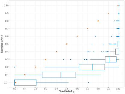
Figure 2: Distribution of the maximum likelihood estimates of $\rho^{\mathrm{CAR}}$ obtained under different realisations of a DAGAR spatial process with different spatial correlations $\rho^{\mathrm{DAGAR}}$, generated the map displayed in Supplementary Figure 2. For every $\rho^{\mathrm{DAGAR}}$, we generated 200 spatial realisations and we estimated the CAR. Red crosses denote the true $\rho^{\mathrm{DAGAR}}$ and have been inserted to help visualising the discrepancy between the true values and the CAR estimates.

The parameters $\tau_{k}$ and $\rho_{k}$ calibrate the spatial distribution of $\boldsymbol{\psi}_{.k}$. The inverse gamma distribution is conjugate with the Gaussian model; therefore, a natural choice of a prior model for $\tau_{k}$ would be $\mathcal{IG}(\alpha_{\tau},\beta_{\tau})$. However, in several tests not shown here, we observed that a Gibbs sampling algorithm for the posterior simulation of $\tau_{k}$ tends to produce highly variable samples. Therefore, we preferred to set $\tau_{k}$ equal a constant (for example, $\tau_{k}=1$ for all $k$). A deeper discussion is required instead for $\rho_{k}$. We already mentioned in Section 2.1 that, under the CAR specification, $\rho_{k}$ does not have any interpretability. Although Datta et al. (2019) conducted several experiments for comparing the DAGAR and the CAR models, they do not show how the CAR retrieves the spatial information of data generated by a DAGAR. We thus simulated a series of spatial datasets using a DAGAR model, based on a map of $n=259$ U.S. counties on the West side of the U.S. map (see Supplementary Figure 2). For every level of spatial correlation used as input (called $\rho^{\mathrm{DAGAR}}$), we produced 200 replicates of the spatial process, and we estimated the CAR model. Figure 2 reports the distribution of the maximum likelihood estimates of $\rho^{\mathrm{CAR}}$ under different $\rho^{\mathrm{DAGAR}}$. We notice that a clear correspondence between the two parameters does not emerge. In fact, when $\rho^{\mathrm{DAGAR}}\geq 0.4$, the distributions of the estimates of $\rho^{\mathrm{CAR}}$ concentrate above 0.9, while, when $0.1\leq\rho^{\mathrm{DAGAR}}\leq 0.3$, the estimates of $\rho^{\mathrm{CAR}}$ span over the whole $(0,1)$ interval. Lastly, when $\rho^{\mathrm{DAGAR}}=0.01$, the most likely value of $\rho^{\mathrm{CAR}}$ appears to be 0.01, although some uncertainty is also evident.

Banerjee et al. (2015) encourage setting $\rho_{k}=1$ when the conditional autoregressive (CAR) prior is used, known as the intrinsic CAR, trusting that the posterior distribution will be proper due to the contribution of the likelihood function. However, under the hierarchical structure of perla, it is not always guaranteed that the posterior distribution of $\boldsymbol{\psi}_{.k}$ is proper, resulting in very unstable results in the phase of posterior inference. To ensure proper posterior distributions, we can fix $\rho_{k}=0.99$ for every $k$, which is the first setup we explore here. Alternatively, we propose inferring $\rho_{k}$ from the data. Carlin and Banerjee (2003) suggest using the prior $\rho_{k}\sim\mathcal{B}(18,2)$, where $\mathcal{B}$ denotes the Beta distribution, to give large probability to values of $\rho_{k}$ close to 1. It is worth noting that the density of this Beta distribution peaks at 0.944 and decreases rapidly as values approach 1, thus discouraging the limit case $\rho_{k}=1$. However, from Figure 2 we observed that, when $\rho^{\mathrm{DAGAR}}$ is particularly low, so is $\rho_{k}$. We thus propose the following mixture prior:

$$\rho_{k}\sim 0.5\mathcal{B}(2,18)+0.5\mathcal{B}(18,2).$$ (6)

We choose a symmetric structure to maintain non-informativeness about the value of $\rho_{k}$, giving equal probability to very small or very high values. The mixture component $\mathcal{B}(2,18)$ reflects the idea of the $\mathcal{B}(18,2)$ component, assigning high probability mass to small values of $\rho_{k}$, while discouraging the case of complete independence $\rho_{k}=0$, which is unusual in spatial data modelling. By placing most of the probability mass toward values close to zero or one - reflecting the almost absence or large presence of spatial correlation - the distribution in (6) retraces the idea of a continuous spike-and-slab prior (Ročková, 2018). Notice also that (6) represents a mixture model that integrates out the mixing probability $\theta_{k}$, whose prior distribution is assumed to be $\theta_{k}\sim\mathcal{B}(c_{\theta},c_{\theta})$, for any $c_{\theta}>0$. One of the goals of the simulation experiments proposed in Section 4 is comparing the two prior proposals for $\rho_{k}$, investigating whether they make any difference in terms of clustering accuracy and model fitting.

We complete the model specification with the prior distributions on $\beta$ and $\boldsymbol{\Sigma}$. We generically assume the conjugate and poorly informative priors ${\beta}_{kj}\sim\mathcal{N}(0,10)$ and $\boldsymbol{\Sigma}\sim\mathcal{IW}(d,\mathbf{I}_{d})$, where $\mathcal{IW}$ denotes the inverse-Wishart distribution.

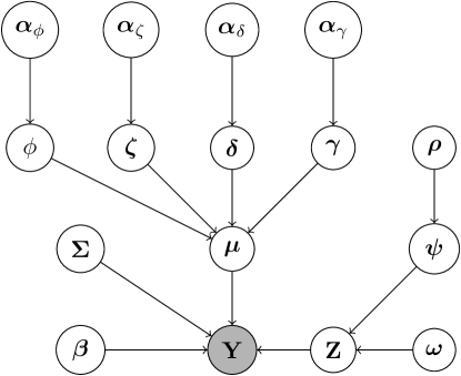
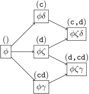
Figure 3: Left: directed acyclic graph (DAG) illustrating the structure of perla with augmented variables. Grey circles represent observed data, while white circles represent random variables. Notice that this graph contains the parameters from both the prior formulations (4) and (5) considered for $\boldsymbol{\mu}$. Hyperparameters are omitted as they have been pre-set. Right: scheme of the combinations of shrinkage factors considered for the prior models of $\boldsymbol{\mu}$. Rectangles contain the shrinkage parameters presented in Formulas (4) and (5). An arrow from A to B means that B is an extension of A. Above the rectangles, we report the notation used in our R package perla. The model (d,cd) corresponds to the prior in (4), (c,d) corresponds to the prior in (5), and (cd) corresponds to the horseshoe prior.

The left panel of Figure 3 illustrates the hierarchical structure of perla through a DAG. Note that this scheme also includes the augmented variables $\boldsymbol{\omega}$, $\boldsymbol{\alpha}_{\phi}$, $\boldsymbol{\alpha}_{\zeta}$, $\boldsymbol{\alpha}_{\delta}$ and $\boldsymbol{\alpha}_{\gamma}$, which will be introduced in the next section to allow the posterior simulation of some model parameters to be performed via Gibbs sampling.

3 Posterior inference

3.1 The MCMC algorithm

We carry out the inference on the model parameters simulating values from their posterior distributions. We present in this section a Markov chain Monte Carlo scheme that allows a direct sampling from the conditional posterior distributions of most of the model parameters, requiring a Metropolis-Hastings step only for a few of them. This translates into the practical advantage of requiring fewer tuning parameters that can be hard to set when either the number of responses $d$ or the number of clusters $K$ grow. With respect to HPM, which requires particular attention for sampling the inverse temperature parameter, our method presents no critical step.

As we already mentioned, the stick-breaking representation in (2) allows to rewrite the multinomial model as a sequence of Bernoulli probability functions. To facilitate the posterior sampling, we introduce the latent variables $\omega_{ik}\sim\mathcal{PG}(N_{ik},0)$, for $k=1,\dots,K-1$ and $i=1,\dots,n$, where $\mathcal{PG}(\cdot,\cdot)$ denotes the Pólya-gamma random variable. Through this data augmentation strategy, we can update the transformed probabilities $\boldsymbol{\psi}_{.k}$ by generating from the conditional posterior distribution of $\boldsymbol{\psi}_{.k}|\omega_{k},\mathbf{Z}_{.k},\rho_{k}$, that is

$$\pi(\boldsymbol{\psi}_{.k}|\omega_{k},\mathbf{Z}_{.k}, \tau_{k},\rho_{k})\propto\left\{\prod_{i=1}^{n}\exp\left(\kappa_{ik}\psi_{ik}-\dfrac{\omega_{ik}\psi^{2}_{ik}}{2}\right)\right\}p(\boldsymbol{\psi}_{.k}|\tau_{k},\rho_{k}),$$

where $\kappa_{ik}=\mathrm{Z}_{ik}-N_{ik}/2$. As the number of spatial areas $n$ grows, and with it the dimension of the neighbour matrix $\mathbf{W}$, it becomes more convenient to update the $\psi_{ik}$ iteratively, rather than generating the full vector $\boldsymbol{\psi}_{.k}$. This can be performed thanks to the Brook’s lemma, which allows to factorise the joint distribution in (3) into a series of univariate conditional distributions derived from the neighbourhood structure imposed by $\mathbf{W}$ (Besag, 1974). The conditional posterior of $\psi_{ik}$ is

$$\psi_{ik}|\boldsymbol{\psi}_{-i,k},\mathbf{Z}_{i.},\omega_{ik},\rho_{k}\sim\mathcal{N}\left\{\varsigma^{2}_{ik}\left(\kappa_{ik}+\dfrac{\rho_{k}}{\tau_{k}}\mathbf{W}^{T}_{i,-i}\boldsymbol{\psi}_{-i,k}\right),\varsigma^{2}_{ik}\right\},$$

where $\varsigma^{2}_{ik}={\tau_{k}}/\left({\tau_{k}\omega_{ik}+D_{ii}}\right)$. The augmented variables $\{\omega_{ik}\}_{ik}$ are updated drawing from $\omega_{ik}|\mathbf{Z}_{i.},\psi_{ik}\sim\mathcal{PG}(\kappa_{ik},\psi_{ik})$ if $N_{ik}=1$, or setting $\omega_{ik}=0$ if $N_{ik}=0$.

The parameter $\rho_{k}$ under the prior model in (6) is the only case for which a closed-form updating scheme is not available. We implemented a random walk Metropolis-Hastings on the transformed parameter $\mathrm{logit}(\rho_{k})$, using a Gaussian distribution centred in the parameter value sampled at the previous iteration, and with variance $\tilde{\sigma}^{2}_{\rho}=3$, in the role of proposal.

To update the clustering labels, it is now sufficient to transform the quantities $\boldsymbol{\psi}_{.1},\dots,\boldsymbol{\psi}_{.K-1}$ into the clustering probabilities $\{{\pi}_{ik}\}_{i,k}$, then drawing a value from the multinomial distribution whose probabilities are defined as

$$\Pr(\mathrm{Z}_{ik}=1|\mathbf{y}_{i.},\boldsymbol{\mu}_{.k},\boldsymbol{\beta}_{.k},{\pi}_{ik},\boldsymbol{\Sigma})\propto\pi_{ik}\mathcal{N}_{d}(\mathbf{y}_{i.}|\boldsymbol{\mu}_{.k}+\mathbf{x}^{T}_{i.}\boldsymbol{\beta},\boldsymbol{\Sigma}),$$

where $\mathcal{N}_{d}(\mathbf{a}|\mathbf{b},\mathbf{C})$ denotes the density of the $d$-variate normal distribution with mean vector $\mathbf{b}$ and covariance matrix $\mathbf{C}$, evaluated in $\mathbf{a}$.

Under the prior model in (4), we update the shrinkage parameters $\boldsymbol{\zeta}$, $\boldsymbol{\gamma}$ and $\phi$ following the data augmentation strategy of Makalic and Schmidt (2016), which exploits the scale mixture representation of the half-Cauchy distribution. We thus introduce a set of augmented scale parameters for each shrinkage parameter considered: $\boldsymbol{\alpha}_{\zeta}=\{\alpha_{\zeta_{j}}\}_{j=1,\dots,d}$, $\boldsymbol{\alpha}_{\gamma}=\{\alpha_{\gamma_{kj}}\}_{j=1,\dots,d,k=1,\dots,K}$, and $\alpha_{\phi}$. Each of these augmented parameters is assumed to distribute according to an inverse gamma $\mathcal{IG}(1/2,1)$. Then, for $j=1,\dots,d$, draw from

$$\alpha_{\zeta_{j}}|\zeta_{j} \sim\mathcal{IG}\left(1,\dfrac{1}{\zeta_{j}}+1\right),\hskip 19.91684pt\zeta_{j}|\boldsymbol{\mu}_{.j},\phi,\boldsymbol{\gamma},\alpha_{\zeta_{j}}\sim\mathcal{IG}\left(\dfrac{K+1}{2},\dfrac{1}{2\phi}\sum_{k=1}^{K}\dfrac{\mu_{kj}^{2}}{\gamma_{kj}}+\dfrac{1}{\alpha_{\zeta_{j}}}\right).$$ (7)

For $k=1,\dots,K$ and $j=1,\dots,d$, draw from

$$\alpha_{\gamma_{kj}}|\gamma_{kj}\sim\mathcal{IG}\left(1,\dfrac{1}{\gamma_{kj}}+1\right),\hskip 19.91684pt\gamma_{kj}|{\mu}_{kj},\phi,\boldsymbol{\zeta},\alpha_{\gamma_{kj}}\sim\mathcal{IG}\left(1,\dfrac{\mu_{kj}^{2}}{2\phi\zeta_{j}}+\dfrac{1}{\alpha_{\gamma_{kj}}}\right).$$ (8)

Lastly, draw from

$$a_{\phi}|\phi\sim\mathcal{IG}\left(1,\dfrac{1}{\phi}+1\right),\hskip 19.91684pt\phi|\boldsymbol{\mu},\boldsymbol{\zeta},\boldsymbol{\gamma},\alpha_{\phi}\sim\mathcal{IG}\left(\dfrac{Kd+1}{2},\sum_{j=1}^{d}\dfrac{1}{2\zeta_{j}}\sum_{k=1}^{K}\dfrac{\mu_{kj}^{2}}{\gamma_{jk}}+\dfrac{1}{\alpha_{\phi}}\right).$$ (9)

Let $\mathcal{C}_{k}=\{i=1,\dots,n:\mathrm{Z}_{ik}=1\}$ be the set denoting which observations belong to cluster $k$. The cluster intercepts are updated drawing from

$$\boldsymbol{\mu}_{k.}|\mathbf{Y}_{\mathcal{C}_{k}.},\boldsymbol{\beta},\boldsymbol{\zeta},\boldsymbol{\delta},\boldsymbol{\gamma},\phi\sim\mathcal{N}_{d}\left[\boldsymbol{\Sigma}^{*}_{k}\left\{\boldsymbol{\Sigma}^{-1}\left(\mathbf{Y}_{\mathcal{C}_{k}.}-\mathbf{X}_{\mathcal{C}_{k}.}\boldsymbol{\beta}\right)\right\},\boldsymbol{\Sigma}^{*}_{k}\right],$$ (10)

where $\boldsymbol{\Sigma}^{*}_{k}=\left[\left\{\phi\;\mathrm{diag}(\zeta_{1}\gamma_{k1},\dots,\zeta_{d}\gamma_{kd})\right\}^{-1}+n_{k}\boldsymbol{\Sigma}^{-1}\right]^{-1}$.

If instead the prior model in (5) is considered, we introduce the set of augmented scale parameters $\boldsymbol{\alpha}_{\delta}=\{\alpha_{\delta_{k}}\}_{k=1,\dots,K}$, each of which distributes according to an inverse gamma $\mathcal{IG}(1/2,1)$. Then, for $k=1,\dots,K$, draw from

$$\alpha_{\delta_{k}}|\delta_{k}\sim\mathcal{IG}\left(1,\dfrac{1}{\delta_{k}}+1\right),\hskip 19.91684pt\delta_{k}|\boldsymbol{\mu}_{k.},\phi,\boldsymbol{\zeta},\alpha_{\delta_{k}}\sim\mathcal{IG}\left(\dfrac{d+1}{2},{\dfrac{1}{2\phi}\sum_{j=1}^{d}\dfrac{\mu_{kj}^{2}}{\zeta_{j}}}+\dfrac{1}{\alpha_{\delta_{k}}}\right).$$

The rest of the updates can be performed as in Formulas (7), (9) and (10), just replacing $\gamma_{kj}$ with $\delta_{k}$.

Finally, the updates of $\boldsymbol{\Sigma}$ and $\boldsymbol{\beta}$ are straightforward to perform, thanks to the conjugancy between the likelihood and the selected priors. Details can be found for example in Marin and Robert (2007).

To provide point estimates of the model parameters, we consider the posterior mode. With the notation $\mathcal{M}(\theta|\mathrm{data})$, we denote the posterior mode of a generic model parameter $\theta$, given the data. A relevant quantity in the analysis of mortality data is also the posterior probability of observing an excess mortality in a specific region, compared to the whole territory. Following the considerations of Richardson et al. (2004), we state that cluster $k$ shows evidence of mortality excess due to disease $j$ if $\Pr(\mu_{kj}>0|\mathrm{data})\geq 0.95$, and a deficit of mortality if $\Pr(\mu_{kj}>0|\mathrm{data})\leq 0.05$. These quantities can be computed straightforwardly from the output of the MCMC algorithm.

3.2 Post-processing and model selection

The presented MCMC scheme is susceptible to the common label-switching phenomenon, which arises due to the unidentifiability of the mixture components and leads the posterior distributions of $\boldsymbol{\mu}$ to be multimodal. In practice, this makes inference on model parameters challenging. To disentangle the mixture components, we explored the ECR algorithm of Papastamoulis and Iliopoulos (2013), considering the partition associated to the largest log-likelihood value as the pivotal one. In addition to this method, the R package label.switching (Papastamoulis, 2016) implements numerous alternative algorithms. Not only are these tools useful to relabel the posterior draws, but they are also designed to return an optimal partition of data based on the MCMC output. This process can also be accomplished using other algorithms, such as the SALSO greedy search method proposed by Dahl et al. (2022).

perla can be fitted with different setups, varying the number of clusters $K$ and the prior distributions of the model parameters. Therefore, a criterion that allows users to evaluate different model setups and determine which is preferable for the analysed data is necessary. This approach aligns with the philosophy of parsimonious clustering (Celeux and Govaert, 1995, Scrucca et al., 2016), which involves comparing the same type of model with different degrees of flexibility and determining the setup that best fits the data.

We conducted the model selection using the $\mathrm{DIC}_{3}$ information criterion of Celeux et al. (2006), which is recommended for mixture models, and whose properties have been studied by Kim (2021). We already discussed in Section 2.2 that different setups for $\boldsymbol{\mu}$ imply different numbers of model parameters. Assuming that the global shrinkage parameter $\phi$ is always inserted into the model, we report in the right panel of Figure 3 the possible combinations of shrinkage factors that we considered for perla, along with the corresponding code notation used in our R package perla. Given the model dimension, users can evaluate all the five combinations of shrinkage factors shown in the figure, starting with simpler models and increasing the complexity. Lastly, it is crucial to underline that model selection cannot rely solely on an information criterion, but must be performed considering also other factors, such as the quality of model fitting, evaluated through the MCMC output, and the interpretability of the clusters.

4 Simulation studies

We studied the performance of perla with two simulation experiments that aim at recreating some possible real data scenarios and conditions. The map used at the base of the simulations is a collection of $n=259$ counties of the U.S. map introduced in Section 1, located West of the 110° W longitude meridian. A representation of this territory is given in Supplementary Figure 2. Every version of perla considered was fitted running the MCMC algorithm four times separately, each for 10,000 iterations, discarding the first half of each run, and merging the remaining draws into a unique chain of length 20,000. Finally, we applied the ECR algorithm to resolve eventual label switching.

4.1 Simulation model

The data generating mechanism that we adopted follows the scheme of perla displayed in the left plot of Figure 3. The only exception is made by the use of the DAGAR prior in place of the CAR to generate the clustering probabilities. This choice allows us to control the amount of spatial correlation simulated in each cluster. The use of the DAGAR requires the ordering of the areas. We thus ordered the counties from the most southern to the most northern. If $i=1,\dots,259$ is the index denoting the counties, then $i=1$ corresponds to the most southern county, and $i=259$ to the most northern. Being $K^{\text{true}}$ the true number of clusters in the map, the simulation model generates the transformed clustering probabilities from

$$\psi^{\text{true}}_{ik}|\boldsymbol{\psi}^{\text{true}}_{\mathscr{N}(i),k}\sim\mathcal{N}\left(\dfrac{\rho^{\text{true}}_{k}}{1+(n_{<i}-1){\rho^{\text{true}}_{k}}^{2}},\dfrac{1-{\rho^{\text{true}}_{k}}^{2}}{1+(n_{<i}-1){\rho^{\text{true}}_{k}}^{2}}\right)$$

where $k=1,\dots,K^{\text{true}}-1$, $\mathscr{N}(i)$ denotes the set of spatial areas that are neighbours of $i$ and precede $i$ according to the imposed ordering, and $n_{<i}=|\mathscr{N}(i)|$. The quantity $\rho^{\text{true}}_{k}\in(0,1)$ denotes the amount of spatial correlation of the probabilities of belonging to cluster $k$. For further details on the DAGAR model, the reader can refer to Datta et al. (2019).

By transforming the quantities $\{\psi^{\text{true}}_{ik}\}_{i=1,\dots,259;k=1,\dots,K^{\text{true}}-1}$ into the clustering probabilities $\{\pi^{\text{true}}_{ik}\}_{i=1,\dots,259;k=1,\dots,K^{\text{true}}}$ through the inverse transformation of the stick-breaking weights, we would obtain highly unbalanced clustering probabilities. To simulate approximately balanced clusters, the inverse transformation of the stick-breaking weights must be applied to $\{\psi^{\text{true}}_{ik}-\log(K-k)\}_{i=1,\dots,259;k=1,\dots,K^{\text{true}}-1}$. Then, the model allocates the spatial areas into clusters, storing the clustering labels into the matrix $\mathbf{Z}^{\text{true}}$. Lastly, given the matrix of centroids $\boldsymbol{\mu}^{\text{true}}$ and the covariance matrix of diseases $\boldsymbol{\Sigma}^{\text{true}}$, the model generates the observed data in the form of the logarithm of mortality rates of $d$ diseases (named also death causes) as

$$\mathbf{y}_{i.}\sim\mathcal{N}_{d}\left\{\left(\mathbf{Z}^{\text{true}}_{i.}\right)^{T}\boldsymbol{\mu}^{\text{true}},\boldsymbol{\Sigma}^{\text{true}}\right\}.$$

In both the simulation experiments that we propose, we took our conclusions using 20 replicates of the data generated under the same experimental conditions.

4.2 Simulation 1

The first simulation experiment serves a dual purpose. On one hand, it examines the gain brought by the use of shrinkage priors, such as those appearing in Formulas (4) and (5), in posterior inference compared to using non-informative priors when the number of diseases considered in the analysis is large. On the other hand, it compares perla with some competing clustering models, such as mixture models and SSS.

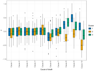
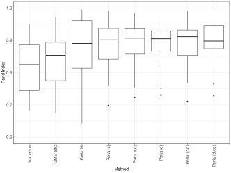
Figure 4: Data and results from Simulation 1. Left: boxplots representing the distribution of the $d=10$ outcomes in the $K^{\text{true}}=3$ clusters in the 20 simulated maps. Death causes 1-5 and 7 are not informative of the clustering structure. Right: boxplots representing the Rand index distribution of several models on the 20 simulated datasets, using $K=4$. ’Perla NI’ denotes the implementation of perla that uses non-informative priors, as discussed at the beginning of Section 4.2.

To accomplish this, we propose a scenario where the formation of mortality clusters is guided only by a subset of the diseases considered. We used $d=10$ diseases and $K^{\text{true}}=3$ clusters. For each of the 20 simulated datasets, we induced large spatial correlation across clustering probabilities, taking ${\rho}^{\text{true}}_{k}\sim\mathcal{U}(0.8,1)$, for $k=1,2$. Next, we randomly determined the diseases that do not contribute to cluster formation: for $j=1,\dots,10$, we introduced a random variable $I_{j}\sim\mathcal{B}e(0.5)$, which takes value 1 if disease $j$ informs the clustering, and 0 if it doesn’t. Then, we drew $\mu^{\text{true}}_{kj}|I_{j}=1\sim\mathcal{U}(-0.5,0.5)$, while we set $\mu_{kj}=0$ if $I_{j}=0$, for all $k$. We generated $\boldsymbol{\Sigma}^{\text{true}}$ by first simulating the correlation values from a uniform $\mathcal{U}(-0.1,0.1)$, and then we multiplied all the elements by a factor of 0.05 to obtain the covariance matrix. The 20 synthetic datasets were finally generated following the simulation model described in Section 4.1. We illustrate the distribution of the outcome variables in one of the 20 datasets in the left panel of Figure 4, where $I_{j}=0$ for $j=1,\dots,5$ and $j=7$.

For each of the 20 scenarios, we fitted the following models:

• perla, with shrinkage factors $\phi\zeta$, $\phi\delta$, $\phi\gamma$, $\phi\zeta\delta$, and $\phi\zeta\gamma$;

• perla, with the non-informative priors $\mu_{kj}\sim\mathcal{N}(0,10)$, for all $k$ and $j$;

• a Gaussian mixture model (GMM), selected with the BIC criterion, using the R library mclust (Scrucca et al., 2016).

• the k-means algorithm, considered also by Aungkulanon et al. (2017);

• the SSS of Gómez-Rubio et al. (2019), implemented in the R library Dclusterm. This algorithm fits a series of generalised linear models using the observed death counts as outcomes, and the expected death counts as offsets. However, our simulation model produces continuous data. Therefore, we applied Dclusterm within a linear regression model, rather than a Poisson regression model. In addition, this method does not handle the analysis of multiple causes of death simultaneously, so it needs to be applied to every disease separately.

To the best of our knowledge, a library software that implements the multivariate HPM is not available in the R computing environment. In addition, the current version of bayesImageS (Moores et al., 2020a) does not fully support non-regular lattice data. This did not allow us to compare perla with HPM.

We applied perla, GMM and k-means using $K=4$ to test how effectively each model can retrieve the clustering structure of data when the number of clusters is incorrectly specified. The right panel of Figure 4 displays the Rand index distribution on the 20 datasets given by each model. Although the perla model setup that should fit better with these data considers the penalisation factors $\phi$ and $\boldsymbol{\zeta}$ (denoted as (d) in the right plot of Figure 3), we notice that, in practice, all the configurations of perla lead to comparable results in terms of classification accuracy. The efficiency of all the shrinkage parameter configurations tested can be explained by the presence of some $\mu^{\text{true}}_{kj}$ whose value is close to 0 for some $k$ even $I_{j}=1$. For example, in the left plot of Figure 4 we see that the distribution of $\{y_{i7}:\mathrm{Z}^{\text{true}}_{i}=3\}$, the death cause 7 in cluster 3, is much closer to zero than the distributions in the two other clusters. Therefore, it is reasonable that the shrinkage parameters $\boldsymbol{\delta}$ and $\boldsymbol{\gamma}$ can provide a relevant contribution to the clustering also in this simulation context. From the obtained results, we see that overall the use of shrinkage priors guarantees substantially less variability in the classification results with respect to using non-informative priors (denoted as ‘Perla NI’). As expected, all the configurations of perla globally perform better than mixture models not informed by the spatial data structure. We do not report the results obtained with the Dclusterm algorithm, as it failed to retrieve the clustering structure in all of the 20 datasets.

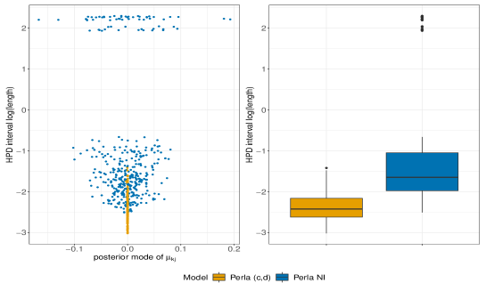
Figure 5: Results from Simulation 1. Left: plot of the $\mu_{kj}$ parameters across the 20 simulated maps for which $I_{j}=0$: the x-axis indicates their posterior modes, and the y-axis the logarithm of their 95% HPD interval length. Different colours denote different versions of perla. Right: boxplots of the distribution of the logarithm of the 95% HPD interval length.

The contribution of shrinkage priors extends beyond overall clustering accuracy to identifying the diseases leading to the formation of clusters. In the left plot of Figure 5, we display the estimated posterior modes and the 95% high posterior density (HPD) intervals of the $\mu_{kj}$ parameters across the 20 simulated maps for which $I_{j}=0$. We compare the results obtained from perla with non-informative priors and from perla (c,d), which achieved the highest median Rand index among all competing models (see right panel of Figure 4). Using the shrinkage prior, the posterior distributions are zero-centred, and the estimated HPD intervals are short. In contrast, when the non-informative prior is employed, the posterior modes are highly variable and the HPD intervals are large. We notice also that, among the estimates provided by ‘Perla NI’, some parameters show a very large HPD interval size. These estimates are associated to the fourth component of the mixture model, which does not find a correspondence with a real cluster. Therefore, while perla with non-informative priors returns highly variable, not zero-centred posterior distributions, the model with shrinkage parameters identifies the presence of a spurious cluster. This result is also evident from the distribution of HPD interval lengths displayed in the right panel of Figure 5. These results contribute to further explain the good performance achieved by perla (c,d) under the simulation framework considered here.

Overall, we conclude that the use of shrinkage priors helps to reduce the variability of posterior estimates and improves the identification of diseases leading to the formation of mortality clusters. We also note that in our simulation experiment, informative diseases are accurately identified by both shrinkage and non-informative priors. This result is illustrated in Supplementary Figure 3.

4.3 Simulation 2

The second simulation experiment aims at studying the performance of perla when the clustering probabilities have different levels of spatial correlation. This setting reflects a scenario where some clusters exhibit strong spatial connection, resulting in geographically concentrated and interconnected areas, while others may show weak spatial connection, with areas scattered across the whole territory.

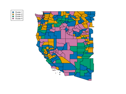
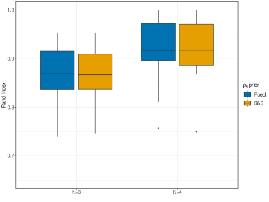
Figure 6: Data and results from Simulation 2. Left: example of a simulated dataset based on the 259 counties of the U.S. West coast divided in $K^{\text{true}}=4$ clusters. Right: boxplots of the Rand indexes on 20 simulated datasets, obtained using two different priors for $\rho_{k}$ and assuming $K\in\{3,4\}$ components.

To accomplish this, we generated 20 simulated maps of mortality rates, considering $d=3$ death causes and $K^{\text{true}}=4$ clusters. To induce different levels of spatial correlation among clustering probabilities, we considered three equispaced values, $\boldsymbol{\rho}^{\text{true}}=(0.01,0.455,0.9)$. These values did not change across the 20 simulation replicates. To induce marginal correlation across causes of death, we generated $\boldsymbol{\Sigma}^{\text{true}}$ by first simulating the correlation values from a uniform $\mathcal{U}(-0.2,0.2)$, and then we multiplied all the elements by a factor of 0.07 to obtain the covariance matrix. We generated the cluster- and disease-specific intercepts $\mu_{kj}$, for $k=1,\dots,4$ and $j=1,2,3$, from $\mathcal{U}(-1,1)$. Lastly, each dataset was drawn from the simulation model detailed in Section 4.1. The left panel of Figure 6 displays one of the 20 simulated scenarios, showing the spatial clusters in the territory. The map shows that the counties in cluster 1 are distributed across the entire territory, while regions in clusters 2 and 3 are more geographically concentrated due to the larger spatial correlation values used in the simulation. Additionally, Supplementary Figure 4 shows for the same dataset the distribution of the three outcomes within each cluster.

In Section 2.2, we already mentioned a possible relation that emerges between the parameters $\rho^{\mathrm{CAR}}$ and $\rho^{\mathrm{DAGAR}}$ and, starting from that, we detailed the prior model in Formula (6) that induces $\rho_{k}$ values either close to 0 or to 1. We consider both the prior setups for $\rho_{k}$ discussed in Section 2.2: the first assumes $\rho_{k}=0.99$ $\forall k$, the second considers the prior (6). We denote the first as ‘Fixed’ and the second as ‘S&S’. The current simulation experiment aims to evaluate whether a more complex prior model for $\rho_{k}$ offers advantages in clustering accuracy and model fitting compared to assuming a constant value, especially when the clustering probabilities exhibit different levels of spatial correlation. Evaluating different prior models for $\mu_{kj}$ is beyond the scope of this simulation; therefore, we fitted only the perla (cd) version of the model, assuming $K=3,4$.

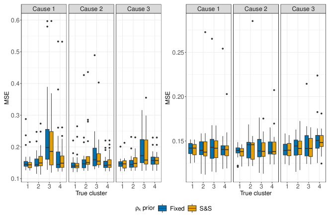
Figure 7: Results from Simulation 2. Boxplots denote the distribution of the MSE within each of the four real clusters and for the three causes of death, using two different priors for $\rho_{k}$. Results are shown for $K=3$ (left) and $K=4$ (right).

The right panel of Figure 6 shows the Rand index distribution across the 20 simulated datasets. We observe that, when the number of clusters is correctly specified, perla accurately recovers the underlying clustering structure (median Rand index $>0.9$). As expected, the performance is generally worse when the number of clusters is misspecified (median Rand index $\in(0.85,0.9)$). Both prior setups perform similarly in terms of clustering accuracy for $K=3$ and $K=4$. We display in Figure 7 the distribution of the mean squared error (MSE) within every real cluster. The scope is evaluating whether the use of different prior models for $\rho_{k}$ lead to different performances in terms of model fitting. We evaluate the MSE within each cluster separately because clusters are characterised by different levels of spatial correlation. When the number of clusters is misspecified, both models struggle to accurately recover the data values in cluster 3 ($\rho^{\text{true}}_{3}=0.9$); however, the S&S model shows a lower median MSE for every cause of death. The models perform similarly in the three remaining clusters. When $K=4$, the MSE values are comparable across clusters and between the two models; except for one case, the median MSE is always below 0.15.

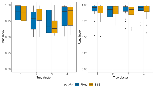
Figure 8: Results from Simulation 2. Boxplots denote the Rand index distribution within each of the four real clusters and for the three causes of death, using two different priors for $\rho_{k}$. Results are shown for $K=3$ (left) and $K=4$ (right).

We also measured the accuracy of recovering each cluster separately. To do so, let $\mathbf{Z}^{\mathrm{post}}$ be the posterior estimate of the matrix $\mathbf{Z}$, which collects the clustering labels. For $k=1,\dots,K^{\text{true}}$, let $h(k)=\arg\max_{\ell=1,\dots,K}\mathrm{Rand}(\mathrm{Z}^{\text{true}}_{.k},\mathrm{Z}^{\mathrm{post}}_{.\ell})$ be the index of estimated clusters most associated with the $k$-th real cluster. Figure 8 displays the distribution of $\mathrm{Rand}(\mathrm{Z}^{\text{true}}_{.k},\mathrm{Z}^{\mathrm{post}}_{.h(k)})$, for every true cluster $k=1,\dots,4$. This graph helps visualise which clusters are more challenging for the model to detect. We observe that, when $K=3$, cluster 3 remains the most challenging to recover. Unlike what we observed with the MSE, the S&S prior performs worse than the Fixed prior. When $K=4$, we do not detect significant differences either across clusters or between models.

We conclude that, when the data-generating mechanism presents several clusters with different levels of spatial correlation, perla performs well in recovering the clustering structure when the number of clusters is correctly specified. In addition, it appears not to be influenced by the varying levels of spatial correlation. On the contrary, when the assumed number of clusters is lower than the true number, both the clustering accuracy and the model fitting are more affected in areas with high spatial correlation. The spike-and-slab-type prior(6) performed slightly better in terms of MSE compared to assuming a constant value for $\rho_{k}$, but it performed worse in recovering the cluster with the highest spatial correlation. Overall, from our simulations it appears that the two prior models for $\rho_{k}$ do not lead to substantially different results.

5 Case studies

In this section, we investigate the existence of mortality clusters in the case studies discussed in Section 1.1. In both scenarios, we applied perla to male and female populations separately, considering all the combinations of shrinkage factors displayed in the right plot of Figure 3, and considering $\rho_{k}=0.99$, $\forall k$. Every model was fitted running the MCMC algorithm four times separately, each for 10,000 iterations, discarding the first half of each run, and merging the remaining draws into a unique chain of length 20,000. Lastly, we applied the ECR algorithm to resolve eventual label switching.

5.1 Mortality in the Padua province

We investigated the presence of mortality clusters in the Padua province using the age-adjusted standardised mortality ratios $SMR_{ij}=O_{i}/E_{i}$, derived as the ratio between observed death counts ($O_{ij}$) and expected death counts ($E_{ij}$) in the $i=1,\dots,106$ areas and for the $j=1,2,3$ diseases considered. The expected number of deaths represents the number of deaths per age class that would occur if the mortality rates per age class of the entire province were applied. Thus, assuming $T$ age classes, the expected number of deaths from disease $j$ in the $i$-th area is $E_{ij}=\sum_{t=1}^{T}n_{it}r_{jt}$, where $r_{jt}$ is the provincial mortality rate of the $j$-th disease of interest within the $t$-th age class, measured in the $i$-th area, and $n_{it}$ is the population size within the $i$-th area and the $t$-th age class. For our analysis, we considered

$$y_{ij}=\log\left(SMR_{ij}\right);$$

the logarithm was applied so that $y_{ij}=0$ represents the case of concordance between observed and expected deaths, $y_{ij}>0$ denotes a mortality excess compared to the regional level, and $y_{ij}<0$ denotes a mortality deficit compared to the regional level.

We considered for the analysis also two variables that are representative of the socioeconomic status of individuals in an area. Specifically, we considered:

• Deprivation index, quantified through the Caranci’s index (Caranci and Costa, 2009). This index quantifies the deprivation, which represents socio-economic disadvantages, by considering various factors affecting residents in the territory. It is calculated as the standardised sum of five indicators, with higher scores indicating higher deprivation (Rosano et al., 2020). These five indicators include the level of education among individuals aged 15-60, the unemployment status, the condition of single-parent family with underage children, house renting and housing density per 100 m². The index typically ranges between $-5$ and 40, with most cases between $-$2 and 2. The data used to compute the index, sourced from the Italian 2011 census, are available at census section level and were aggregated to obtain data at municipality level.

• Sale price of real estate per squared meter, which serves as an indicator of the general economic status of municipalities. These price data were scraped from www.immobiliare.it, a web portal that collects property sales listings in Italy, using the average of the prices in €/m² on January 1${}^{\makebox{st}}$ of 2017, 2018, and 2019 (immobiliare.it, 2022). The specific time frame was chosen as it is characterised by stable price trends, without notable increases or decreases.

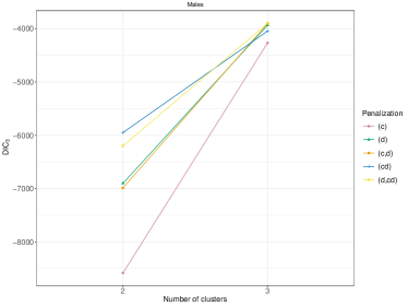
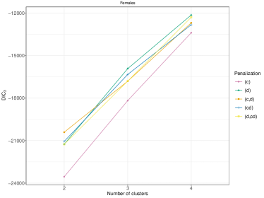
Figure 9: Model selection results on the male and female mortality data in the Padua province. X-axis represents the number of clusters considered, y-axis reports the $\mathrm{DIC}_{3}$ values, and the different shapes indicate the models with different shrinkage factors for $\mu_{kj}$.

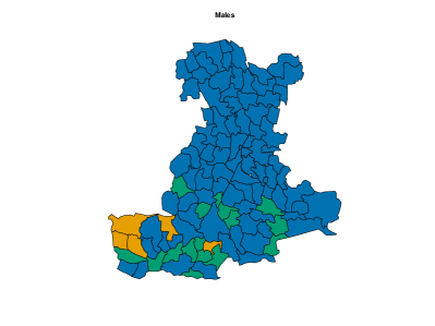
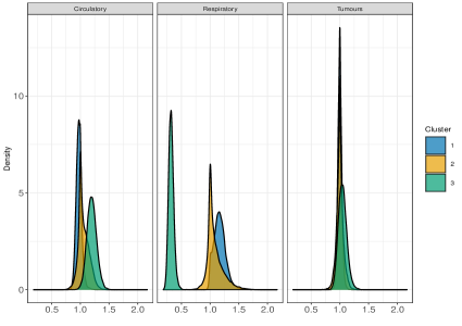
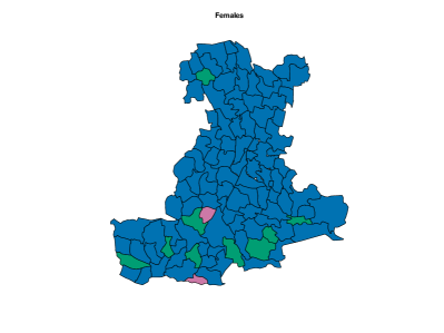
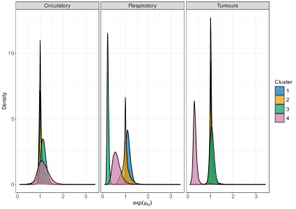
Figure 10: Results on the Padua province data, divided for males (top line) and females (bottom line). Left plots display the 106 areas of the Padua province coloured according to the best partition returned by the ECR relabelling algorithm. Right plots display the posterior densities of the $\{\mu_{kj}\}$, based on 20,000 posterior draws, obtained from the model with $K=3$ (males) and $K=4$ (females).

On male data, we fitted perla considering $K=2$ and $K=3$, mainly motivated by the relatively small number of areas in the map. Results of the model selection are shown in Figure 9. The $\mathrm{DIC}_{3}$ criterion clearly supports $K=2$, and, either under $K=2$ or $K=3$, it suggests considering the model with only the cluster specific shrinkage (c). However, the plot of the posterior distribution of $\boldsymbol{\mu}$ under $K=2$ (top panel of Supplementary Figure 5) displays multiple modes, which is a clear indication that a model with an additional component should be considered. We thus applied perla with $K=3$ and shrinkage factor (c). The final classification of the map is reported in the top-left plot of Figure 10. While cluster 1 extends over the whole territory, particularly on the northern area of the province, clusters 2 and 3 are located in the south-west. The posterior densities of $\{\exp(\mu_{kj})\}_{kj}$ are displayed in the top-right panel of Figure 10, showing that cluster 1 is characterised by an excess mortality due to respiratory diseases ($\mathcal{M}(\mu_{12}|\mathrm{data})=1.156$, $\Pr\{\exp(\mu_{12})>1|\mathrm{data}\}=0.973$), and cluster 3 by a mortality excess due to circulatory diseases ($\mathcal{M}(\mu_{31}|\mathrm{data})=1.182$, $\Pr\{\exp(\mu_{31})>1|\mathrm{data}\}=0.994$) and by a mortality deficit due to respiratory diseases ($\mathcal{M}(\mu_{32}|\mathrm{data})=0.322$, $\Pr\{\exp(\mu_{32})>1|\mathrm{data}\}=0$). Lastly, cluster 2 does not show evidence of neither excess nor deficit of mortality due to the three causes of death considered. In Table 1, we report all the posterior SMR estimates and the probabilities of observing an excess mortality. Notice also that, according to our model, deaths for tumours appear not to impact on the formation of spatial mortality clusters.

On female data, we initially considered the model with 3 clusters, following the conclusions taken from male data. However, since the posterior distribution of $\boldsymbol{\mu}$ under $K=3$ displays multiple modes (see the bottom panel of Supplementary Figure 5), we applied perla with $K=4$ and shrinkage factor (c). The final classification of the map is displayed in the bottom-left plot of Figure 10. Some differences emerge with respect to male data. cluster 3 is geographically located in the same area of the one identified through male data, but its composition is rather different, including a municipality in the northern province. Additionally, the model detects a fourth cluster consisting of only two separate municipalities. The posterior densities of $\{\exp(\mu_{kj})\}_{kj}$ are displayed in the bottom-right plot of Figure 10, and detailed estimates are reported in the bottom part of Table 1. In female population, we detect an excess mortality in the northern province due to respiratory diseases, and a deficit of mortality for the same causes in cluster 3 and 4. In addition, cluster 4 is characterised by a non-negligible deficit of mortality due to tumours. cluster 3 shows also a probability of excess mortality due to circulatory diseases of almost 0.9.

Although cluster 4 comprises only two municipalities, there is strong evidence of its separation from cluster 3. Supplementary Figure 6 illustrates the percentage of times each pair of municipalities in clusters 3 and 4 were assigned to the same cluster across the MCMC iterations. The estimated probability that the two municipalities finally assigned to cluster 4 (Barbona and Arquà Petrarca) belong to the same cluster exceeds 0.9. In contrast, the estimated probability of either municipality being placed in the same cluster with any of the nine municipalities finally assigned to cluster 3 ranges from 0 to 0.05.

We notice also that the best partition selected by the ECR algorithm does not include cluster 2. Observations assigned to cluster 2 in some MCMC iterations are all part of the group of 95 observations denoted as cluster 1 in the final estimate of the data partition. We conclude that, although cluster 2 does not have a practical epidemiological interpretation, its inclusion in some MCMC iterations helped achieve unimodal posterior distributions, facilitating the inference on the model parameters and the computation of some quantities of interest, such as the probability of mortality excess. Lastly, it is worth to underline that the data partition shown in the bottom-left panel of Figure 10 is equivalent to the partition returned by the SALSO algorithm, confirming the robustness of the results discussed.

Both male and female mortality data do not show substantial evidence of marginal correlation across the three causes of death considered (see the posterior modes and the 95% HPD intervals in Supplementary Table 1).

5.2 Mortality in the U.S. counties

We now investigate the presence of mortality clusters in the U.S. from 2016 to 2019. Due to the high diversity of the U.S. territory already mentioned in Section 1.1, we restricted our attention to the north-east and central-east coasts, selecting the U.S. counties whose centroids are located East of the 80° W longitude meridian. This territory is made of 388 counties, which are displayed in the bottom row of Figure 1. We examined the relative mortality risks ${RR}_{ij}=MR_{ij}/MR_{j}$, derived as the ratio between the age-adjusted mortality rate ($MR_{ij}$) and the total age-adjusted mortality rate ($MR_{j}$) in the $i=1,\dots,388$ counties and for the $j=1,2,3$ diseases considered. These rates were obtained from the Centres for Disease Control and Prevention (CDC) WONDER Online Databases CDC (2021). Assuming $T$ age classes, the age-adjusted mortality rates in county $i$ were computed as $MR_{ij}=\sum_{t=1}^{T}MR_{ijt}P_{t}/P$, where $P$ represents the standard population – the U.S. population in 2000 – $P_{t}$ is the standard population in the $t$-th age class, and $MR_{ijt}$ is the age-specific mortality rate in the $t$-th age class. Similarly, $MR_{j}=\sum_{t=1}^{T}MR_{jt}P_{t}/P$, where $MR_{jt}$ is the age-specific mortality rate in the $t$-th age class over the entire U.S. territory. Due to privacy considerations, some counties present missing data. For counties with less than 10 deceased persons due to a specific death cause, the number of observed deaths and the corresponding mortality rate for that specific death cause are not reported in the WONDER data. In particular, the mortality level due to respiratory causes was not available for the male population in Tyrrell County (NC) and Grand Isle County (VT), and it was unavailable for both male and female populations in Highland County (VA). In such cases, we imputed the missing data using the average mortality rates for the same death cause from neighbouring and bordering counties.

In our analysis, we applied

$$y_{ij}=\log\left(RR_{ij}\right),$$

so that $y_{ij}=0$, $y_{ij}>0$ and $y_{ij}<0$ represent respectively the cases where the mortality in county $i$ due to disease $j$ is equal, larger or smaller than the mortality across the entire U.S. territory.

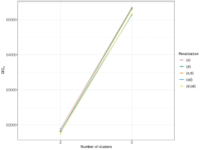
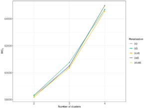
Figure 11: Model selection results on the male and female mortality data in the U.S. East coast. X-axis represents the number of clusters considered, y-axis reports the $\mathrm{DIC}_{3}$ values, and the different shapes indicate the models with different shrinkage factors for $\mu_{kj}$.

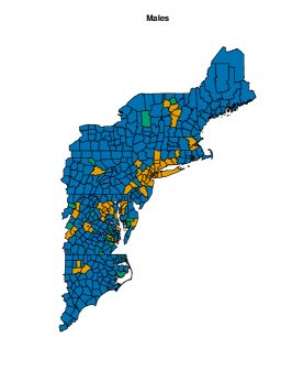
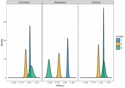
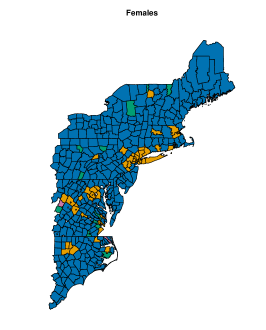
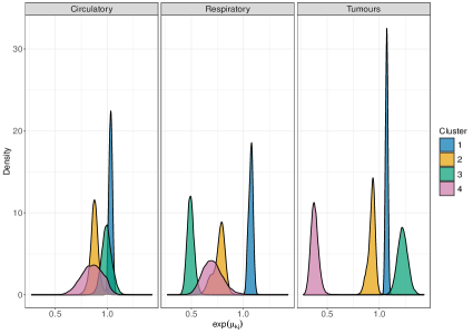
Figure 12: Results on the U.S. East coast data, divided for males (top line) and females (bottom line). Left plots display the 388 counties coloured according to the best partition returned by the ECR relabelling algorithm. Right plots display the posterior densities of the $\{\mu_{kj}\}$, based on 20,000 posterior draws, obtained from the model with $K=3$ (males) and $K=4$ (females).

On male data, we chose the model with $K=3$ clusters and the disease-specific penalisation factor (d). Since all the models were comparable in terms of $\mathrm{DIC}_{3}$ value (see the left panel of Figure 11), we selected the model that provided also unimodal posterior distribution of $\boldsymbol{\mu}$. Results are shown in the top row of Figure 12. A predominant cluster that spans the entire territory is characterised by elevated mortality rates for all causes of death considered. The second cluster comprises primarily large urban areas or their neighbouring counties (including Boston, New York, Long Island, Philadelphia, Baltimore, and the urban area around Washington D.C.), along with some isolated regions. Mortality levels in these areas are uniformly below 1, indicating lower mortality compared to the entire U.S. territory. Lastly, the third cluster consists of isolated counties, showing a mortality deficit for respiratory diseases and a mortality excess for tumours. Further details are provided in Table 2. It also appears that the marginal correlation across causes of death is not negligible. The posterior estimates and the corresponding HPD intervals of the marginal correlations are: 0.438 (0.323,0.546) between circulatory and respiratory causes, 0.417 (0.31,0.51) between circulatory causes and tumours, and 0.339 (0.238,0.466) between respiratory causes and tumours.

On female data, we selected the model with the disease-specific (d) and the cluster- and disease-specific (cd) penalisation factors, taking $K=4$. The results displayed in the bottom row of Figure 12 reveal a spatial distribution of the clusters that mirrors the patterns observed in the male data. Once again, cluster 1 spans the entire territory, cluster 2 captures prevalently large urban areas, and cluster 3 consists of isolated counties. Additionally, cluster 4 comprises only two counties. The posterior distributions in the bottom-right plot illustrate the variations in mortality levels across clusters. The mortality rates for circulatory and respiratory diseases observed in cluster 4 are similar to those in cluster 2, while mortality rate for tumours is substantially lower. Unlike the male data, there is also a mortality excess due to tumours in cluster 3. Further details are provided in the bottom section of Table 2. In comparison to males, the marginal correlations with tumours appear to be lower in female data. The posterior estimates and corresponding 95% HPD intervals are: 0.301 (0.168, 0.432) between circulatory and respiratory causes, 0.357 (0.239, 0.453) between circulatory causes and tumours, and 0.37 (0.264, 0.486) between respiratory causes and tumours.

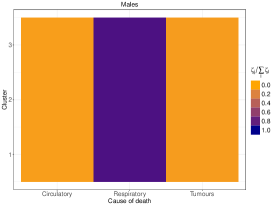
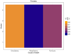
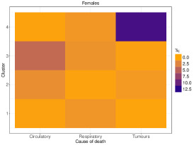
Figure 13: Posterior estimates of the shrinkage factors obtained on U.S. data. Each panel represents a $K\times d$ matrix coloured according to the posterior mode of the shrinkage factors. The top row refers to the results on male data, the bottom row refers to the results on female data. When the parameter $\zeta_{j}$ is considered (for $j=1,\dots,d$), we display its normalised version $\zeta_{j}/\sum_{l=1}^{d}\zeta_{l}$.

Figure 13 displays the posterior estimates of the shrinkage factors employed by the models used for the analysis of male (top row) and female (bottom row) data. Each figure represents a $K\times d$ matrix, coloured according to the posterior mode of the shrinkage factors. The larger the value in the $kj$-th cell, the more significant the contribution of disease $j$ to the formation of the $k$-th cluster. The results for $\zeta_{j}$ are displayed as the normalised version $\zeta_{j}/\sum_{l=1}^{d}\zeta_{l}$, which can be interpreted as the percentage contribution of disease $j$ to the clustering structure. For male data, the clustering is predominantly characterised by differences in mortality levels due to respiratory diseases, which account for approximately 90% of the cluster formation. This is further evidenced by the top row of Table 2, where the variability in risk levels across different clusters is much higher for respiratory diseases than for the other two causes of death. For female data, respiratory diseases account for approximately 50%, and tumours for about 40%. The second panel related to female data shows the joint effects $\gamma_{kj}$. Although this quantity cannot be normalised as $\zeta_{j}$ was, it indicates that tumours are particularly responsible for the formation of cluster 4, and circulatory diseases significantly contribute to the formation of cluster 3.

The two clusters denominated cluster 1 for both male and female data encompass the majority of counties on the map and exhibit higher mortality rates compared to the entire U.S. territory. The absence of spatial clusters reflecting national mortality levels raised concerns about potential systematic biases in the data. Therefore, we conducted an additional analysis in a geographically distant area. Specifically, we applied perla to female data from the 259 counties on the West side map of the U.S., which is the territory used for the simulation experiments detailed in Section 4. The prior setup considered is the same used for the East coast female data. In this region, 27 areas had at least one missing data point and their value was imputed similarly to the missing data on the East coast territory. The analysis revealed the presence of a predominant cluster characterised by lower mortality rates for circulatory diseases and tumours compared to the national average. The remaining two clusters did not correspond to major urban areas as observed in the East coast data; instead, they included regions with low population densities. Detailed plots are provided in Supplementary Figure 7. We conclude that the U.S. East coast exhibits higher mortality levels for major causes of death compared to the rest of the nation, while the West coast demonstrates generally lower mortality levels.

6 Discussion

The analysis of the mortality level distribution due to multiple causes of death provides an overview of the health conditions and disparities within a territory. In particular, detecting mortality clusters allows for identifying areas with similar characteristics and investigating the presence of unknown risk factors. In this work, we propose perla, a multivariate Bayesian model designed to address the dual problem of detecting spatial mortality clusters by simultaneously analysing multiple causes of death and identifying the diseases responsible for cluster formation. perla integrates the spatial structure of data directly into the clustering probabilities, enabling tractable posterior distributions. Additionally, it accounts for the presence of external covariates, if available.

We proposed different setups for perla considering different types of global-local shrinkage priors. These setups help the model distinguish between relevant and spurious clusters, and to identify which death causes are associated with different clusters. The several prior setups allow for the selection of an appropriate level of shrinkage while maintaining parsimony, i.e., without excessively increasing the number of model parameters.

Through two different case-studies, we demonstrated the various insights achievable with our methodology. Not only does our model partition the areas of a territory into clusters, but it also estimates the probability of risk excess in each cluster for each cause of death. Additionally, the model quantifies the marginal correlation across different causes of death. Finally, the inference on the shrinkage parameters allows us to quantify the impact of multiple diseases on the formation of clusters and identifies if some diseases are particularly related to specific clusters.

Although this article has introduced a comprehensive solution to address some key questions in the analysis of multivariate areal data, we believe that there is space for further extensions. While we assumed that the data $\mathbf{Y}$ are realisations of continuous and zero-centred variables, the mortality data often come in the form of counts. Consequently, following the approach of Green and Richardson (2002), the regression specified in Formula (1) could be extended to the generalised linear model framework. So far, our model has been applied in contexts with a small number of exogenous variables $p$. Nonetheless, when $p$ grows substantially, it would be reasonable to use a prior distribution on $\mathbf{B}$ that induces variable selection. This approach should be performed considering the $d$ regressions jointly, as suggested by Deshpande et al. (2019). In the case-studies treated in this work, we performed the model selection looking both at the $\mathrm{DIC}_{3}$ information criterion and the quality of the MCMC samples, preferring models with unimodal posterior distributions. However, this approach necessitates running the perla model multiple times. Alternatively, a simulation algorithm such as the reversible jump Markov chain Monte Carlo (RJMCMC, Green 1995) could streamline this process. RJMCMC would test multiple model setups and provide a probabilistic assessment of the number of clusters and the optimal combination of penalisation parameters that best fit the data. Finally, as we previously mentioned, inference on the parameters can be performed easily via MCMC methods, thanks to multiple data augmentation strategies that allow for expressing most conditional posterior distributions in closed form. These computational characteristics make it possible to explore potentially more efficient estimation procedures, such as variational Bayes methods, which are particularly appealing for the analysis of massive datasets.

7 Supplementary material

Contains additional figures and tables related to both the simulation experiments and case studies.

8 Software

perla has been implemented as an R package, which can be accessed online at https://github.com/andreasottosanti/perla. This package ensures full reproducibility of the analyses conducted on both simulated data and the publicly available mortality U.S. data. Data from the Italian health care system are not accessible due to privacy concerns.

9 Competing interests

No competing interest is declared.

10 Funding

This work was supported by Next Generation EU, in the context of the National Recovery and Resilience Plan, Investment PE8 – Project Age-It: “Ageing Well in an Ageing Society”, CUP C93C22005240007 [DM 1557 11.10.2022]. The views and opinions expressed are only those of the authors and do not necessarily reflect those of the European Union or the European Commission. Neither the European Union nor the European Commission can be held responsible for them. Additionally, GB and PB acknowledge funding from PRIN SOcial and health Frailty as determinants of Inequality in Aging. (SOFIA), project n. 020KHSSKE, CUP C93C22000270001, directorial decree ministry of university n. 222 dated February 18, 2022.

11 Acknowledgments

The authors are thankful to C. Castiglione (Bocconi University) and P. Onorati (University of Padua) for the helpful discussions about global-local shrinkage priors, and to F. Denti (University of Padua) for precious suggestions after reading the first draft of the manuscript. The authors extend their gratitude to B. Bezzon (University of Padua) for linguistic support. Authors also acknowledge ULSS6 Euganea, particularly L. Benacchio, for providing the aggregated SMRs used in this study, within the framework of the STHEP (State of Health in Padua) collaboration between ULSS6 Euganea and the Department of Statistical Sciences of the University of Padua.

		Circulatory ($j=1$)	Respiratory ($j=2$)	Tumours ($j=3$)
Males	$k=1$	1.000 (0.269)	1.156 (0.973)	1.000 (0.462)
	$k=2$	1.001 (0.713)	0.998 (0.72)	1.000 (0.483)
	$k=3$	1.182 (0.994)	0.322 (0.000)	1.06 (0.726)
Females	$k=1$	1.001 (0.461)	1.098 (0.953)	1.001 (0.69)
	$k=2$	1.000 (0.588)	1.002 (0.523)	0.999 (0.637)
	$k=3$	1.154 (0.898)	0.229 (0.000)	1.042 (0.768)
	$k=4$	1.061 (0.704)	0.614 (0.034)	0.295 (0.003)

Table 1: Results on the Padua province, divided for males and females. Each cell of the table displays the posterior modal value of $\exp(\mu_{kj})$ and the probability of observing a mortality excess $\Pr\{\exp(\mu_{kj})>1|\mathrm{data}\}$. Values for which the probability of mortality excess is larger than 0.95 or smaller than 0.05 are reported in bold.

		Circulatory ($j=1$)	Respiratory ($j=2$)	Tumours ($j=3$)
Males	$k=1$	1.04 (0.996)	1.097 (1)	1.1 (1)
	$k=2$	0.897 (0.001)	0.811 (0.000)	0.927 (0.002)
	$k=3$	1.093 (0.927)	0.478 (0.000)	1.092 (0.995)
Females	$k=1$	1.034 (0.975)	1.079 (1)	1.072 (1)
	$k=2$	0.878 (0.007)	0.793 (0.000)	0.939 (0.006)
	$k=3$	0.998 (0.445)	0.494 (0.000)	1.22 (1)
	$k=4$	0.883 (0.067)	0.707 (0.004)	0.374 (0.000)

Table 2: Results on the U.S. East coast data, divided for males and females. Each cell of the table displays the posterior modal value of $\exp(\mu_{kj})$ and the probability of observing a mortality excess $\Pr\{\exp(\mu_{kj})>1|\mathrm{data}\}$. Values for which the probability of mortality excess is larger than 0.95 or smaller than 0.05 are reported in bold.

References

- Ahmed and Genin (2020) Mohamed-Salem Ahmed and Michaël Genin. A functional-model-adjusted spatial scan statistic. Statistics in Medicine, 39(8):1025–1040, 2020. ISSN 1097-0258. doi: 10.1002/sim.8459.
- Amini et al. (2023) Maedeh Amini, Mehdi Azizmohammad Looha, Sajjad Rahimi Pordanjani, Hamid Asadzadeh Aghdaei, and Mohamad Amin Pourhoseingholi. Global long-term trends and spatial cluster analysis of pancreatic cancer incidence and mortality over a 30-year period using the global burden of disease study 2019 data. PloS One, 18(7), 2023.
- Aungkulanon et al. (2017) Suchunya Aungkulanon, Viroj Tangcharoensathien, Kenji Shibuya, Kanitta Bundhamcharoen, and Virasakdi Chongsuvivatwong. Area-level socioeconomic deprivation and mortality differentials in Thailand: results from principal component analysis and cluster analysis. International journal for equity in health, 16:1–12, 2017.
- Banerjee et al. (2015) Sudipto Banerjee, Bradley P. Carlin, and Alan E. Gelfand. Hierarchical modeling and analysis for spatial data, volume 135 of Monographs on Statistics and Applied Probability. CRC Press, Boca Raton, FL, second edition, 2015. ISBN 978-1-4398-1917-3.
- Besag (1974) Julian Besag. Spatial Interaction and the Statistical Analysis of Lattice Systems. Journal of the Royal Statistical Society. Series B (Methodological), 36(2):192–236, 1974. ISSN 0035-9246.
- Bhadra et al. (2019) Anindya Bhadra, Jyotishka Datta, Nicholas G. Polson, and Brandon Willard. Lasso Meets Horseshoe: A Survey. Statistical Science, 34(3):405–427, 2019. ISSN 0883-4237.
- Bovo et al. (2023) Enrico Bovo, Pietro Belloni, Andrea Sottosanti, and Giovanna Boccuzzo. Territorial clusters of mortality and role of social and environmental factors: the case of ULSS 6 Euganea (Italy). In 2023 IEEE Conference on Computational Intelligence in Bioinformatics and Computational Biology (CIBCB), pages 1–5. IEEE, 2023.
- Caranci and Costa (2009) Nicola Caranci and Giuseppe Costa. Un indice di deprivazione a livello aggregato da utilizzare su scala nazionale: giustificazioni e composizione. Salute e società. Fascicolo 1, 2009, pages 1000–1021, 2009.
- Carlin and Banerjee (2003) Bradley P. Carlin and Sudipto Banerjee. Hierarchical Multivarite CAR Models for Spatio-Temporally Correlated Survival Data. Bayesian Statistics, 7(7):45–63, 2003.
- Carvalho et al. (2010) Carlos M. Carvalho, Nicholas G. Polson, and James G. Scott. The horseshoe estimator for sparse signals. Biometrika, 97(2):465–480, 2010. ISSN 0006-3444.
- CDC (2021) CDC. National vital statistics system, mortality 1999-2020 on cdc wonder online database, 2021. Accessed on: Apr 11, 2024. http://wonder.cdc.gov/mcd-icd10.html.
- Celeux et al. (2006) G. Celeux, F. Forbes, C. P. Robert, and D. M. Titterington. Deviance information criteria for missing data models. Bayesian Analysis, 1(4):651–673, 2006. ISSN 1936-0975, 1931-6690. doi: 10.1214/06-BA122.
- Celeux and Govaert (1995) Gilles Celeux and Gérard Govaert. Gaussian parsimonious clustering models. Pattern Recognition, 28(5):781–793, 1995. ISSN 0031-3203. doi: 10.1016/0031-3203(94)00125-6.
- Coker et al. (2023) Eric S Coker, John Molitor, Silvia Liverani, James Martin, Paolo Maranzano, Nicola Pontarollo, and Sergio Vergalli. Bayesian profile regression to study the ecologic associations of correlated environmental exposures with excess mortality risk during the first year of the Covid-19 epidemic in Lombardy, Italy. Environmental Research, 216, 2023.
- Cucala (2016) Lionel Cucala. A Mann–Whitney scan statistic for continuous data. Communications in Statistics - Theory and Methods, 45(2):321–329, January 2016. ISSN 0361-0926. doi: 10.1080/03610926.2013.806667.
- Cucala et al. (2017) Lionel Cucala, Michaël Genin, Caroline Lanier, and Florent Occelli. A multivariate Gaussian scan statistic for spatial data. Spatial Statistics, 21:66–74, August 2017. ISSN 2211-6753. doi: 10.1016/j.spasta.2017.06.001.
- Cucala et al. (2019) Lionel Cucala, Michaël Genin, Florent Occelli, and Julien Soula. A multivariate nonparametric scan statistic for spatial data. Spatial Statistics, 29:1–14, March 2019. ISSN 2211-6753. doi: 10.1016/j.spasta.2018.10.002.
- Dahl et al. (2022) David B. Dahl, Devin J. Johnson, and Peter Müller. Search Algorithms and Loss Functions for Bayesian Clustering. Journal of Computational and Graphical Statistics, 31(4):1189–1201, 2022. ISSN 1061-8600. doi: 10.1080/10618600.2022.2069779.
- Datta et al. (2019) Abhirup Datta, Sudipto Banerjee, James S. Hodges, and Leiwen Gao. Spatial Disease Mapping Using Directed Acyclic Graph Auto-Regressive (DAGAR) Models. Bayesian Analysis, 14(4), 2019. ISSN 1936-0975. doi: 10.1214/19-BA1177.
- Deshpande et al. (2019) Sameer K. Deshpande, Veronika Ročková, and Edward I. George. Simultaneous Variable and Covariance Selection With the Multivariate Spike-and-Slab LASSO. Journal of Computational and Graphical Statistics, 28(4):921–931, 2019. ISSN 1061-8600. doi: 10.1080/10618600.2019.1593179.
- Fedeli et al. (2021) Ugo Fedeli, Elena Schievano, Francesco Avossa, Tiziana Baruffa, Adriano Rampado, Alessandro Lucia, Marco Veronese, Nicola Gennaro, Michele Pellizzari, Elisabetta Pinato, Eliana Ferroni, Cristina Basso, Silvia Tiozzo Netti, Laura Cestari, Angela De Paoli, Matilde Dotto, Silvia Pierobon, Veronica Casotto, Marica Costa, Marco Braggion, Maria Rosaria Lamattina, and Velentina Zabeo. La mortalità nella Regione del Veneto. periodo 2016-2019, 2021.
- Frévent et al. (2023) Camille Frévent, Mohamed-Salem Ahmed, Sophie Dabo-Niang, and Michaël Genin. Investigating spatial scan statistics for multivariate functional data. Journal of the Royal Statistical Society Series C: Applied Statistics, 72(2):450–475, May 2023. ISSN 0035-9254. doi: 10.1093/jrsssc/qlad017.
- Green (1995) Peter J. Green. Reversible jump Markov chain Monte Carlo computation and Bayesian model determination. Biometrika, 82(4):711–732, 1995. ISSN 0006-3444. doi: 10.1093/biomet/82.4.711.
- Green and Richardson (2002) Peter J. Green and Sylvia Richardson. Hidden Markov Models and Disease Mapping. Journal of the American Statistical Association, 97(460):1055–1070, 2002. ISSN 0162-1459.
- Griffith (2023) Daniel A Griffith. Spatial autocorrelation mixtures in geospatial disease data: An important global epidemiologic/public health assessment ingredient? Transactions in GIS, 27(3):730–751, 2023.
- Gómez-Rubio et al. (2019) Virgilio Gómez-Rubio, Paula Moraga, John Molitor, and Barry Rowlingson. DClusterm: Model-Based Detection of Disease Clusters. Journal of Statistical Software, 90:1–26, August 2019. ISSN 1548-7660. doi: 10.18637/jss.v090.i14.
- immobiliare.it (2022) immobiliare.it. Real estate price data in Italy, 2022. Accessed on: Dec 19, 2022. https://www.immobiliare.it/mercato-immobiliare.
- Kim (2021) Chanmin Kim. Deviance information criteria for mixtures of distributions. Communications in Statistics - Simulation and Computation, 50(10):2935–2948, 2021. ISSN 0361-0918. doi: 10.1080/03610918.2019.1617878.
- Kulldorff (1997) Martin Kulldorff. A spatial scan statistic. Communications in Statistics-Theory and methods, 26(6):1481–1496, 1997.
- Kulldorff et al. (2005) Martin Kulldorff, Richard Heffernan, Jessica Hartman, Renato Assunçao, and Farzad Mostashari. A space–time permutation scan statistic for disease outbreak detection. PLoS medicine, 2(3):e59, 2005.
- Künzli et al. (2000) N Künzli, R Kaiser, S Medina, M Studnicka, O Chanel, P Filliger, M Herry, F Horak, V Puybonnieux-Texier, P Quénel, J Schneider, R Seethaler, J-C Vergnaud, and H Sommer. Public-health impact of outdoor and traffic-related air pollution: a European assessment. The Lancet, 356(9232):795–801, September 2000. ISSN 0140-6736. doi: 10.1016/S0140-6736(00)02653-2.
- Lafferty and Blei (2005) John Lafferty and David Blei. Correlated Topic Models. In Advances in Neural Information Processing Systems, volume 18. MIT Press, 2005.
- Lawson (2013) Andrew B Lawson. Statistical methods in spatial epidemiology. John Wiley & Sons, 2013.
- Lee et al. (2009) Duncan Lee, Claire Ferguson, and Richard Mitchell. Air pollution and health in Scotland: a multicity study. Biostatistics, 10(3):409–423, 2009.
- Li et al. (2012) Guangquan Li, Nicky Best, Anna L. Hansell, Ismaïl Ahmed, and Sylvia Richardson. BaySTDetect: detecting unusual temporal patterns in small area data via Bayesian model choice. Biostatistics, 13(4):695–710, 2012. ISSN 1465-4644. doi: 10.1093/biostatistics/kxs005.
- Li et al. (2021) Yihao Li, Danh V. Nguyen, Sudipto Banerjee, Connie M. Rhee, Kamyar Kalantar-Zadeh, Esra Kürüm, and Damla Şentürk. Multilevel Modeling of Spatially Nested Functional Data: Spatiotemporal Patterns of Hospitalization Rates in the U.S. Dialysis Population. Statistics in medicine, 40(17):3937–3952, July 2021. ISSN 0277-6715. doi: 10.1002/sim.9007.
- Linderman et al. (2015) Scott W. Linderman, Matthew J. Johnson, and Ryan P. Adams. Dependent multinomial models made easy: stick breaking with the Pólya-gamma augmentation. In Proceedings of the 28th International Conference on Neural Information Processing Systems - Volume 2, NIPS’15, pages 3456–3464, Cambridge, MA, USA, 2015. MIT Press.
- Liu et al. (2018) Ying Liu, Yawen Liu, and Tonglin Zhang. Wald-based spatial scan statistics for cluster detection. Computational Statistics & Data Analysis, 127:298–310, November 2018. ISSN 0167-9473. doi: 10.1016/j.csda.2018.06.002.
- Makalic and Schmidt (2016) Enes Makalic and Daniel F. Schmidt. A Simple Sampler for the Horseshoe Estimator. IEEE Signal Processing Letters, 23(1):179–182, 2016. ISSN 1558-2361. doi: 10.1109/LSP.2015.2503725.
- Marin and Robert (2007) Jean-Michel Marin and Christian P. Robert. Regression and Variable Selection. In Bayesian Core: A Practical Approach to Computational Bayesian Statistics, pages 47–84. Springer, New York, NY, 2007. ISBN 978-0-387-38983-7.
- McGrory et al. (2009) C. A. McGrory, D. M. Titterington, R. Reeves, and A. N. Pettitt. Variational Bayes for estimating the parameters of a hidden Potts model. Statistics and Computing, 19(3):329–340, 2009. ISSN 1573-1375. doi: 10.1007/s11222-008-9095-6.
- Moores et al. (2020a) Matthew Moores, Geoff Nicholls, Anthony Pettitt, and Kerrie Mengersen. Scalable Bayesian Inference for the Inverse Temperature of a Hidden Potts Model. Bayesian Analysis, 15(1):1–27, 2020a. ISSN 1936-0975, 1931-6690. doi: 10.1214/18-BA1130.
- Moores et al. (2015) Matthew T. Moores, Christopher C. Drovandi, Kerrie Mengersen, and Christian P. Robert. Pre-processing for approximate Bayesian computation in image analysis. Statistics and Computing, 25(1):23–33, 2015. ISSN 1573-1375. doi: 10.1007/s11222-014-9525-6.
- Moores et al. (2020b) Matthew T. Moores, Anthony N. Pettitt, and Kerrie L. Mengersen. Bayesian Computation with Intractable Likelihoods. In Kerrie L. Mengersen, Pierre Pudlo, and Christian P. Robert, editors, Case Studies in Applied Bayesian Data Science: CIRM Jean-Morlet Chair, Fall 2018, pages 137–151. Springer International Publishing, Cham, 2020b. ISBN 978-3-030-42553-1.
- Papastamoulis (2016) Panagiotis Papastamoulis. label.switching: An R Package for Dealing with the Label Switching Problem in MCMC Outputs. Journal of Statistical Software, 69:1–24, 2016. ISSN 1548-7660. doi: 10.18637/jss.v069.c01.
- Papastamoulis and Iliopoulos (2013) Panagiotis Papastamoulis and George Iliopoulos. On the Convergence Rate of Random Permutation Sampler and ECR Algorithm in Missing Data Models. Methodology and Computing in Applied Probability, 15(2):293–304, 2013. ISSN 1573-7713. doi: 10.1007/s11009-011-9238-7.
- Polson and Scott (2011) Nicholas G. Polson and James G. Scott. Shrink Globally, Act Locally: Sparse Bayesian Regularization and Prediction. In José M. Bernardo, M. J. Bayarri, James O. Berger, A. P. Dawid, David Heckerman, Adrian F. M. Smith, and Mike West, editors, Bayesian Statistics 9, page 0. Oxford University Press, October 2011. ISBN 978-0-19-969458-7.
- Potts (1952) R. B. Potts. Some generalized order-disorder transformations. Mathematical Proceedings of the Cambridge Philosophical Society, 48(1):106–109, 1952. ISSN 1469-8064, 0305-0041. doi: 10.1017/S0305004100027419.
- Qian et al. (2023) Qi Qian, Danh V Nguyen, Donatello Telesca, Esra Kurum, Connie M Rhee, Sudipto Banerjee, Yihao Li, and Damla Senturk. Multivariate spatiotemporal functional principal component analysis for modeling hospitalization and mortality rates in the dialysis population. Biostatistics, 2023.
- R Core Team (2024) R Core Team. R: A Language and Environment for Statistical Computing. R Foundation for Statistical Computing, Vienna, Austria, 2024. URL https://www.R-project.org/.
- Richardson et al. (2004) Sylvia Richardson, Andrew Thomson, Nicky Best, and Paul Elliott. Interpreting Posterior Relative Risk Estimates in Disease-Mapping Studies. Environmental Health Perspectives, 112(9):1016–1025, 2004. doi: 10.1289/ehp.6740.
- Robertson et al. (2010) Colin Robertson, Trisalyn A. Nelson, Ying C. MacNab, and Andrew B. Lawson. Review of methods for space–time disease surveillance. Spatial and Spatio-temporal Epidemiology, 1(2):105–116, July 2010. ISSN 1877-5845. doi: 10.1016/j.sste.2009.12.001.
- Rosano et al. (2020) Aldo Rosano, Barbara Pacelli, Nicolas Zengarini, Giuseppe Costa, Cesare Cislaghi, and Nicola Caranci. Aggiornamento e revisione dell’indice di deprivazione italiano 2011 a livello di sezione di censimento. Epidemiologia e Prevenzione, 44(2-3):162–70, 2020.
- Ročková (2018) Veronika Ročková. Bayesian estimation of sparse signals with a continuous spike-and-slab prior. The Annals of Statistics, 46(1):401–437, February 2018. ISSN 0090-5364, 2168-8966. doi: 10.1214/17-AOS1554.
- Russo et al. (2022) Massimiliano Russo, Burton H. Singer, and David B. Dunson. Multivariate mixed membership modeling: Inferring domain-specific risk profiles. The Annals of Applied Statistics, 16(1):391–413, 2022. ISSN 1932-6157. doi: 10.1214/21-aoas1496.
- Scrucca et al. (2016) Luca Scrucca, Michael Fop, T. Brendan Murphy, and Adrian E. Raftery. mclust 5: Clustering, Classification and Density Estimation Using Gaussian Finite Mixture Models. The R journal, 8(1):289–317, 2016. ISSN 2073-4859.
- Tango (2021) Toshiro Tango. Spatial scan statistics can be dangerous. Statistical Methods in Medical Research, 30(1):75–86, 2021.
- Taylor et al. (2015) Jonathon Taylor, Paul Wilkinson, Mike Davies, Ben Armstrong, Zaid Chalabi, Anna Mavrogianni, Phil Symonds, Eleni Oikonomou, and Sylvia I Bohnenstengel. Mapping the effects of urban heat island, housing, and age on excess heat-related mortality in london. Urban Climate, 14:517–528, 2015.
- Tesema et al. (2023) Getayeneh Antehunegn Tesema, Zemenu Tadesse Tessema, Stephane Heritier, Rob G Stirling, and Arul Earnest. A systematic review of joint spatial and spatiotemporal models in health research. International Journal of Environmental Research and Public Health, 20(7):5295, 2023.
- van Erp et al. (2019) Sara van Erp, Daniel L. Oberski, and Joris Mulder. Shrinkage priors for Bayesian penalized regression. Journal of Mathematical Psychology, 89:31–50, April 2019. ISSN 0022-2496. doi: 10.1016/j.jmp.2018.12.004.
- Waller and Gotway (2004) Lance A Waller and Carol A Gotway. Applied spatial statistics for public health data. John Wiley & Sons, 2004.
- Wong et al. (2008) Chit-Ming Wong, Nuntavarn Vichit-Vadakan, Haidong Kan, Zhengmin Qian, and the PAPA Project Teams. Public Health and Air Pollution in Asia (PAPA): A Multicity Study of Short-Term Effects of Air Pollution on Mortality. Environmental Health Perspectives, 116(9):1195–1202, September 2008. doi: 10.1289/ehp.11257.
- Zhao et al. (2021) Edward Zhao, Matthew R. Stone, Xing Ren, Jamie Guenthoer, Kimberly S. Smythe, Thomas Pulliam, Stephen R. Williams, Cedric R. Uytingco, Sarah E. B. Taylor, Paul Nghiem, Jason H. Bielas, and Raphael Gottardo. Spatial transcriptomics at subspot resolution with BayesSpace. Nature Biotechnology, 39(11):1375–1384, 2021. ISSN 1546-1696. doi: 10.1038/s41587-021-00935-2.
- Zhu and Fan (2023) Wanchuang Zhu and Yanan Fan. A synthetic likelihood approach for intractable markov random fields. Computational Statistics, 38(2):749–777, 2023. ISSN 1613-9658. doi: 10.1007/s00180-022-01256-x.