Rates and beaming angles of GRBs associated with compact binary coalescences

Abstract

Some, if not all, binary neutron star (BNS) coalescences, and a fraction of neutron - star black hole (NSBH) mergers, are thought to produce sufficient mass-ejection to power Gamma-Ray Bursts (GRBs). However, this fraction, as well as the distribution of beaming angles of BNS-associated GRBs, are poorly constrained from observation. Recent work applied machine learning tools to analyze GRB light curves observed by Fermi/GBM and Swift/BAT. GRBs were segregated into multiple distinct clusters, with the tantalizing possibility that one of them (BNS cluster) could be associated with BNSs and another (NSBH cluster) with NSBHs. As a proof of principle, assuming that all GRBs detected by Fermi/GBM and Swift/BAT associated with BNSs (NSBHs) lie in the BNS (NSBH) cluster, we estimate their rates ($\mathrm{Gpc}^{-3}\mathrm{yr}^{-1}$). We compare these rates with corresponding BNS and NSBH rates estimated by the LIGO-Virgo-Kagra (LVK) collaboration from the first three observing runs (O1, O2, O3). We find that the BNS rates are consistent with LVK’s rate estimates, assuming a uniform distribution of beaming fractions ($f_{b}\in[0.01,0.1]$). Conversely, using the LVK’s BNS rate estimates, assuming all BNS mergers produce GRBs, we are able to constrain the beaming angle distribution to $\theta_{j}\in[0.8^{\circ},38.8^{\circ}]$ at $90\%$ confidence. We similarly place a lower limit on the fraction of GRB-Bright NSBHs to $f_{B}\gtrsim 0.10$ ($f_{B}\gtrsim 0.022$) with Fermi/GBM (Swift/BAT) data.

1 Introduction

The LIGO-Virgo-Kagra detector network (Aasi et al., 2015; Acernese et al., 2015; Akutsu et al., 2021) has observed $\sim 90$ compact binary coalescences (CBCs) during its first three observing runs (O1, O2, O3) (Abbott et al., 2023a). Among these, only two were binary neutron star (BNS) mergers (Abbott et al., 2017a, 2020), of which only one (GW170817) produced an observed kilonova and Gamma-Ray Burst (GRB) (Abbott et al., 2017b). Two neutron star - black hole mergers (NSBHs) were also detected, but no corresponding EM counterparts were observed (Abbott et al., 2021a).

The prevalent expectation is that some, if not all, BNS mergers produce EM counterparts, including GRBs (Paczynski, 1986a; Narayan et al., 1991; Chatterjee et al., 2020). On the other hand, not all NSBH mergers are expected to produce such counterparts (see, e.g. Foucart, 2020, and references therein). A necessary (though not sufficient) condition for producing these counterparts is a non-zero remnant mass post-merger (Foucart, 2012). Intuitively, if the tidal forces on the NS from the BH are sufficiently large, then the NS can disrupt outside the innermost stable circular orbit (ISCO) of the BH, which in turn will leave a non-zero remnant mass.

Such a requirement imposes a restriction on the mass-ratios $q$ of the NSBH that could allow such an extra-ISCO NS disruption, although the exact $q$ values ultimately depend on the equation of state of the NS, and the spin of the BH (Foucart et al., 2018). Nevertheless, lower mass ratios (with the mass ratio defined such that $q\in[1,\infty)$) are more likely to produce EM-counterparts (Foucart et al., 2013), including GRBs, though their occurrence is not guaranteed given the complexities associated with the physics of jet production (see, e.g. Salafia et al., 2020).

Testing standard assumptions about GRB-Bright CBCs ideally requires multiple confident joint GW-GRB detections, of which there is a severe paucity (Abbott et al., 2022, 2021b, 2019; Burns et al., 2019). However, a number of GRBs have been detected by the gamma-ray burst monitor (GBM) on board the Fermi satellite, as well as the Burst Alert Telescope (BAT) of the Swift satellite. GRBs are typically classified into long and short GRBs, based on the duration $T_{90}$ for $90\%$ of the energy in prompt emission to be released. The provenance of long GRBs (lGRBs, $T_{90}>2s$) has traditionally been attributed to collapsars (collapse of massive stars) (Woosley, 1993; Paczyński, 1998; Mészáros, 2006; Woosley & Bloom, 2006; Hjorth & Bloom, 2012), while short GRBs (sGRBs, $T_{90}<2s$) are thought to be produced by CBCs (Paczynski, 1986b; Eichler et al., 1989; Meszaros & Rees, 1992). These assumptions have been supported by observations of broad-lined Type Ic supernovae (SNe) coincident with lGRBs (Galama et al., 1998; Kulkarni et al., 1998; Stanek et al., 2003; Cano et al., 2017), and r-process nucleosynthesis driven Kilonovae (KNe) associated with sGRBs (Berger et al., 2013; Tanvir et al., 2013; Kasliwal et al., 2017; Abbott et al., 2017; Valenti et al., 2017; Troja et al., 2019; Lamb et al., 2019).

However, some GRB events were found to violate standard expectations. Examples include GRB 200826A, which was a sGRB with an SN counterpart (Ahumada et al., 2021; Zhang et al., 2021), GRBs 060614 and 060505 were lGRBs with no observed SNe associated with them (Fynbo et al., 2006), and GRBs 060614 (Yang et al., 2015) and 211227A (Lü et al., 2022) which were long but data suggested evidence of coincident KNe. Indeed, even data from the observations of high-redshift sGRBs suggest collapsars as potential progenitors of these events (Dimple et al., 2022).

Recently, GRB 211211A had a prolonged burst phase with an associated KN (Rastinejad et al., 2022). Several models have been proposed to suggest its provenance, most of which point to a CBC-origin (Yang et al., 2022; Gompertz et al., 2023; Troja et al., 2022; Zhu et al., 2022; Zhong et al., 2023; Kunert et al., 2024). This conclusion is further corroborated by the host galaxy whose properties coincided with those pertaining to hosts of sGRBs (Troja et al., 2022; Yang et al., 2022). Moreover, the GRB’s location with respect to the host’s center seemed to suggest a lack of spatial coincidence with any star forming region, which again points to a CBC progenitor rather than a collapsar origin (Fruchter et al., 2006; Berger et al., 2013). More recently, JWST observations of the bright lGRB 230307a also indicated the presence of a potential KN (Sun et al., 2023; Levan et al., 2024).

It is, therefore, amply evident that the standard picture of sGRB + KN + CBC and lGRB + SN + collapsar cannot be reconciled with data that increasingly suggests a more complex picture. A more sophisticated approach to segregating GRBs into groups and subgroups belonging to a collapsar origin or a CBC origin and to further split the CBC group into a BNS or NSBH cluster is to use machine learning (ML). Several works have attempted this, where light curves from the prompt emission phase of GRBs detected by one instrument are fed to an unsupervised ML algorithm that identifies global structures (Jespersen et al., 2020; Steinhardt et al., 2023; Luo et al., 2023; Garcia-Cifuentes et al., 2023). Recently, Dimple et al. (2023) identified five distinct clusters in the Swift/BAT GRB population, with KN-associated GRBs located in two separate clusters. This structure remains true for both the catalogs – Swift/BAT as well as for Fermi/GBM (Dimple et al., 2024). They suggested that these two distinct populations might be associated with BNS and/or NSBH mergers. One cluster with KN-associated GRBs having longer $T_{90}$’s might be associated with NSBH mergers (Zhu et al., 2022). On the other hand, the presence of GRB 170817A in the other cluster (Dimple et al., 2024) confirms that at least a fraction of GRBs in that cluster might be associated with BNS mergers.

While there is some uncertainty on whether all GRBs that sit in either of these two clusters can be associated with a BNS or NSBH, it is still interesting to estimate the rate of BNS/NSBH- associated GRBs, assuming that such GRBs must lie in these two clusters. In this Letter, we evaluate these rates, and compare them to the BNS and NSBH rates reported by the LVK in its first three observing runs (O1, O2, O3) (Abbott et al., 2023b). We find that the rate of BNS-associated GRBs are broadly consistent with the BNS-associated GW rate estimates. We additionally constrain the fraction of GRB-bright NSBHs, and, assuming that all BNSs produce GRBs, the beaming angle of BNS-associated GRBs.

2 Method

2.1 Estimating the Rate of GRBs

Most works that estimate the rate of GRBs assume a model for the redshift evolution, which is typically chosen to be the Madau-Dickinson ansatz (Madau & Dickinson, 2014; Madau & Fragos, 2017) pertaining to star formation rate. While this model may be sufficient for GRBs thought to originate from collapsars, a model for the rate of CBC-driven GRBs needs to additionally account for a delay time between the formation of the compact binary and its coalescence (Wanderman & Piran, 2015). This is usually achieved by adopting an additional ansatz on the distribution of delay times, although there are considerable uncertainties in the models of delay-time distributions.

On the other hand, the rate of BNS and NSBH mergers estimated by the LVK ($R_{\rm GW}$), given GW data ($d_{\rm GW}$), is limited by the relative scarcity of BNS/NSBH-associated GW detections (Abbott et al., 2023a). Moreover, the confirmed BNS/NSBH-associated GW detections are at relatively low redshifts, making it difficult to probe their redshift evolution. We therefore similarly evaluate an aggregated rate of BNS/NSBH-associated GRBs ($R_{\rm GRB}$) assuming that the sources are distributed uniformly in comoving volume, as done in Appendix C of Abbott et al. (2023b), Abbott et al. (2021a), and Kapadia et al. (2020). This will allow for a self-consistent evaluation of the fraction of GRB-Bright NSBHs, as well as the beaming angle of BNS-associated GRBs.

Consider $N_{\rm GRB}$ GRB detections collected over an observation time $T_{\rm obs}$. We make two assumptions. The first is that the GRB detections are independent and, therefore, follow a Poisson process. The second is that the intrinsic luminosity function of the GRBs, $p_{L}(L)$, has no redshift dependence.

The first assumption allows us to write down the Poisson likelihood as (we remove the GRB subscript to reduce notational burden):

$$p(N|\Lambda)=\frac{1}{N!}\Lambda^{N}\exp(-\Lambda).$$ (1)

The posterior on the Poisson mean is found using Bayes’ rule: $p(\Lambda|N)\propto p(\Lambda)p(N|\Lambda)$. The posterior on the rate of GRBs, $R=\frac{\Lambda}{\langle VT\rangle}$, is then:

$$p(R|N)\propto p(\Lambda|N)=p(R\cdot\langle VT\rangle|N)$$ (2)

The task now is to estimate the spacetime volume sensitivity, $\langle VT\rangle$ of the GRB detector, averaged over the expected distribution of fluxes $p_{F}(F)$ accessible to the detector. This sensitivity is given by:

$$\langle VT\rangle=T_{\rm obs}\cdot\int_{0}^{\infty}\frac{1}{1+z}\frac{dV_{c}}{dz}f(z)dz$$ (3)

where $\frac{dV_{c}}{dz}$ is the differential comoving volume, $\frac{1}{1+z}$ accounts for cosmological time dilation, and $f(z)$ is the fraction of spacetime volume accessible to the detector (with threshold flux $F_{t}$) given by:

$$f(z)=\int_{F_{t}}^{\infty}p_{F}(F)dF$$ (4)

By definition, the flux $F$ and the intrinsic luminosity $L$ of the source are related by:

$$F=\frac{L}{4\pi d_{L}^{2}}$$ (5)

where $d_{L}$ is the luminosity distance. The flux function can then be written in terms of the intrinsic luminosity function ($p_{L}(L)$), and $f(z)$ is evaluated as:

$$f(z)=4\pi d_{L}^{2}(z)\int_{F_{t}}^{\infty}p_{L}(4\pi d_{L}^{2}(z)F)dF$$ (6)

Let $f_{b}$ be the beaming fraction, $f_{s}$ be the fraction of the sky viewed by the detector at any given time, and $f_{k}$ the K-correction factor due to redshifting and finite bandwidth of the Fermi detector. The spacetime volume sensitivity accessible to the instrument is then Eq. (3) multiplied by these fractions. Since the beaming fractions, especially for sGRBs, are poorly constrained from observation (Fong et al., 2015), we draw them from a broad, uninformative prior distribution.

To estimate the beaming fraction of BNS-associated GRBs, we assume that all BNS mergers produce GRBs. This may be justified by the high extent of tidal disruption possible in BNS mergers compared to, say, NSBH mergers. The disruption provides enough matter near the merger site to produce an accreting central engine that can power the jet.

We then evaluate the ratio distribution $p(\langle f_{b}\rangle\equiv\frac{R_{\rm GRB}}{R_{\rm GW}}|N_{\rm GRB},d_{\rm GW})$, pertaining to BNSs. This distribution is constructed from the GRB ($p(R_{\rm GRB}|N_{\rm GRB})$) and GW ($p(R_{\rm GW}|d_{\rm GW})$) rate posteriors. We ensure that $R_{\rm GRB}$ is evaluated with $\langle VT\rangle$ using Eq. (3), without multiplying it by an assumed $f_{b}$. This ratio distribution constrains the average beaming fraction $\langle f_{b}\rangle$.

From the ratio distribution, we evaluate constraints on the minimum ($f_{b}^{\mathrm{min}}$) and maximum ($f_{b}^{\mathrm{max}}$) beaming fractions, assuming a uniform distribution $f_{b}\in\mathcal{U}(f_{b}^{\mathrm{min}},f_{b}^{\mathrm{max}})$. We do so using Monte Carlo, and by exploiting the fact that $\langle f_{b}\rangle=(f_{b}^{\mathrm{min}}+f_{b}^{\mathrm{max}})/2$. We draw from $p(\langle f_{b}\rangle|N_{\rm GRB},d_{\rm GW})$. For each $\langle f_{b}\rangle$ sample, we draw an $f_{b}^{\mathrm{min}}$ sample from a uniform distribution $\mathcal{U}(0,\langle f_{b}\rangle)$. We then acquire an $f_{b}^{\mathrm{max}}$ sample as $f_{b}^{\mathrm{max}}=2\langle f_{b}\rangle-f_{b}^{\mathrm{min}}$. Repeating this process iteratively, we construct distributions for $f_{b}^{\mathrm{min}}$ and $f_{b}^{\mathrm{max}}$.

The beaming angle ($\theta_{j}$) is acquired from the beaming fraction via:

$$f_{b}=1-\cos(\theta_{j})$$ (7)

The constraint on the fraction of GRB-Bright NSBHs, $f_{B}$ is similarly acquired from a ratio distribution pertaining to NSBHs, but now assuming a prior distribution on $f_{b}$.

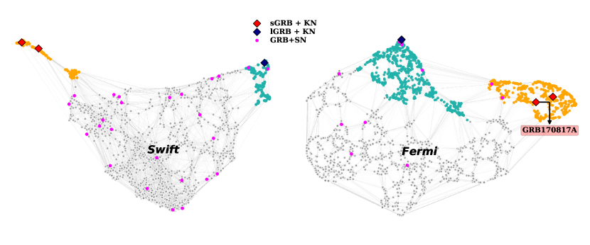
Figure 1: Two-dimensional embeddings obtained using PCA-UMAP for Swift/BAT and Fermi/GBM catalogs. The red squares show the locations of KN-associated lGRBs. The blue squares show the locations of KN-associated sGRBs. GRB 170817A is highlighted in the red label, suggesting the origin of neighboring GRBs to be BNS mergers. Therefore, we assume clusters highlighted in orange to be a BNS cluster, while those in cyan to be an NSBH cluster. The SN-associated GRBs are represented by the magenta color circles. Notice that some of these clusters contain known false-positives. (See Dimple et al. 2024, 2023 for details.)

2.2 Progenitor Identification with Machine Learning

To estimate BNS/NSBH-associated GRB rates, it is crucial to first identify, from the set of GRBs detected by an instrument, those that can be associated with a BNS or an NSBH. Dimple et al. (2023) used machine learning algorithms, particularly uniform manifold approximation and projection (UMAP, McInnes et al., 2018), and t-distributed stochastic neighbor embedding (Maaten, 2008; Van Der Maaten, 2014), with a principle component analysis (PCA) initialization on GRB light curves in Swift/BAT, to achieve this. Although working on different principles, both algorithms separated the KN-associated GRBs into two distinct clusters. This suggested two distinct populations of KN-associated GRBs, one associated with sGRBs and the other with lGRBs. Further inspection suggested they might have different origins (see Figure 4 in Dimple et al. 2023).

The association of clusters with a BNS or NSBH provenance becomes stronger with data from the Fermi/GBM catalog (Dimple et al., 2024). Figure 1 shows the 2-dimensional embeddings obtained using PCA-UMAP on Swift/BAT and Fermi/GBM light curves. The one KN-associated sGRB event, detected by Fermi, whose BNS provenance is beyond all “reasonable” doubt, GW170817’s counterpart, GRB 170817A, lies within what we call the “BNS cluster” in the embedding. This implies that some fraction of GRBs in that cluster might originate from BNS mergers. For GRBs in the other “NSBH cluster”, some have coincident KNe and evidence of fallback accretion. This suggests that NSBH mergers could be progenitors (Zhu et al., 2022) for at least a fraction of the GRBs in this cluster. However, only multimessenger observations of NSBH coalescences can confirm this prediction.

While not confirmed, we nevertheless still work with the assumption that all BNS/NSBH- associated GRBs in the data set (from Fermi or Swift) have been identified and placed in the BNS/NSBH clusters. However, not all events in these clusters have a BNS/NSBH provenance. Some known SNe also lie in these clusters. We account for this when estimating BNS/NSBH-associated GRB rates, as delineated in the following subsection.

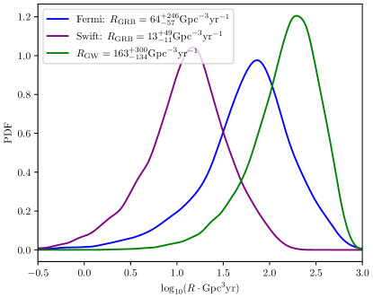
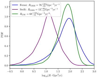
Figure 2: Left Panel: The posteriors on the rate of GRB-Bright BNS mergers, $p(R_{\mathrm{GRB}}|\mathcal{N}_{\mathrm{BNS}})$, estimated using Fermi data and Swift data. These are both broadly consistent with GW BNS rate posterior $p(R_{\mathrm{GW}}|d_{\mathrm{GW}})$. The $90\%$ rate estimates are quoted on the top left corner of the panel. The larger errorbar on the Fermi rate estimates can be attributed to the larger uncertainty in the fraction of events in the BNS cluster that have a BNS provenance, as compared to the Swift rate estimates. Right Panel: Same as the Left Panel, but for NSBHs. As with the BNS rate posteriors, these are broadly consistent with each other, with errorbars on the Fermi rate estimates being larger than those on the Swift rate estimates.

2.3 Counting Error Estimation

Let $n$ be the total number of events in the BNS or NSBH cluster. Of these, let $N_{\mathrm{KN}}$ be the number of known KNe and let $N_{\mathrm{SN}}$ be the number of known SNe. We wish to evaluate the probability that there are $N$ KNe in the cluster, given that $N$ could lie anywhere between $N_{\mathrm{KN}}\leq N\leq n-N_{\mathrm{SN}}$:

$$p(N|\mathcal{N}),~{}~{}\mathcal{N}\equiv N_{\mathrm{KN}}\leq N\leq n-N_{\mathrm{SN}}$$ (8)

From Bayes’ theorem:

$$p(N|\mathcal{N})=\frac{p(\mathcal{N}|N)p(N)}{p(\mathcal{N})}$$ (9)

The prior $p(N)$ is assumed to be uniform for $N$ satisfying $\mathcal{N}$, and zero otherwise. The likelihood can be written as:

$$p(\mathcal{N}|N)=\int_{0}^{1}p(\mathcal{N}|q)p(q|N)dq$$ (10)

where $q$ is the probability that an individual event is a KN, which is unknown. From Bayes’ theorem:

$$p(q|N)\propto p(N|q)p(q)$$ (11)

Assuming $p(N|q)$ is Binomially distributed, and a uniform prior on $q$, we get, after normalisation:

$$p(q|N)=\frac{q^{N}(1-q)^{n-N}}{\beta(N+1,n-N+1)}$$ (12)

where the function in the denominator is the Euler Beta function.

On the other hand, it is straightforward to see that:

$$p(\mathcal{N}|q)=1-\sum_{j=0}^{N_{\mathrm{KN}}-1}B(j;n,q)-\sum_{j=0}^{N_{\mathrm{SN}}-1}B(n-j;n,q)$$ (13)

where $B(j;n,q)$ is the usual Binomial distribution with $j$ successful trials. Thus, $p(N|\mathcal{N})$ can be evaluated from Eqs. 9, 10, 12, and 13.

The posterior on the Poisson mean is then convolved with $p(N|\mathcal{N})$, thereby incorporating counting uncertainties:

$$p(\Lambda|\mathcal{N})=\sum_{N=0}^{n}p(\Lambda|N)p(N|\mathcal{N})$$ (14)

3 Results and Discussion

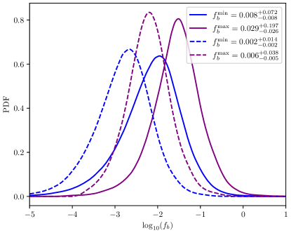
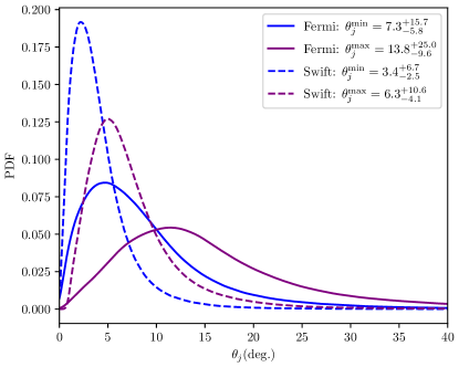
Figure 3: Left Panel: Constraints on the distribution of beaming fractions for GRBs with a BNS provenance, assuming that all BNSs produce GRBs. The constraints from Fermi are less stringent than those from Swift. The reason is the same as what was described in Figure 2 to explain the broader rate posteriors for Fermi as compared to Swift. Right Panel: Distributions of beaming fractions in the Left Panel converted to distributions of beaming angles $\theta_{j}$ (in $\degree$). These span $\theta_{j}\in[0.8\degree,38.8\degree]$ across both Fermi and Swift estimates.

We present the results of our estimates of the rate of BNS/NSBH-associated GRBs. Using Fermi data (Von Kienlin et al., 2020), with $T_{\rm obs}=15.22~{}{\rm yrs}$, the ML classification scheme of Dimple et al. (2024) identifies $n=593$ ($716$) events in the BNS (NSBH) cluster, of which $2$ ($2$) are known to be KNe, and $2$ ($10$) are known to be SNe. Similarly, using Swift data (Lien et al., 2016), with $T_{\rm obs}=18.8~{}{\rm yrs}$, $n=117$ ($115$) events are placed in the BNS (NSBH) cluster, of which $3$ ($3$) are known to be KNe, and $0$ ($4$) are known to be SNe.

We use these numbers to estimate the posterior on the Poisson mean $\Lambda$, $p(\Lambda|\mathcal{N})$, as described in the previous section. We then convert this posterior to one on the rate by evaluating the spacetime volume sensitivity $\langle VT\rangle$.

We use Eq. 3 to estimate $\langle VT\rangle$, assuming a flux threshold $F_{t}$ of $2\times 10^{-7}\mathrm{ergs}/\mathrm{s}/\mathrm{cm}^{2}$ ($5\times 10^{-8}\mathrm{ergs}/\mathrm{s}/\mathrm{cm}^{2}$) for Fermi/GBM (Swift/BAT). We assume a broken power-law profile for the luminosity function $p_{L}(L)$, as done in Wanderman & Piran (2015):

$$\phi(L)=\begin{cases}\left(\frac{L}{L_{b}}\right)^{-a},&\text{if $L\leq L_{b}$}.\\ \left(\frac{L}{L_{b}}\right)^{-b},&\text{if $L>L_{b}$}.\end{cases}$$ (15)

where $\phi(L)$ traditionally denotes the number of samples between $\log_{10}(L)$ and $\log_{10}(L)+d\log_{10}(L)$ (Wanderman & Piran, 2010), and can be straightforwardly related to $p_{L}(L)$. The shape parameters of the broken power-law function estimated by Wanderman & Piran (2015) are $a=0.95^{+0.12}_{-0.12}$, $b=2.0^{+1.0}_{-0.8}$, and $L_{b}=2.0^{+1.4}_{-0.4}\times 10^{52}$ ergs/s. We construct a distribution on $\langle VT\rangle$ by approximating the errors on the shape parameters as Gaussians, and drawing from these Gaussians assuming that the values provided pertain to medians and upper/lower limits at $1\sigma$ confidence. We also consider a uniform distribution of $f_{b}\in[0.01,0.10]$. Moreover, we take the K-correction factor as $f_{K}=1.13$ (Poolakkil et al., 2021) and sky fraction to be $f_{s}=2/3$ ($f_{s}=1/6$) for Fermi/GBM (Swift/BAT).

We draw $10^{4}$ samples from $p(\Lambda|\mathcal{N})$ and the $\langle VT\rangle$ distribution, and divide sample by sample to estimate the GRB rate posterior $p(R_{\mathrm{GRB}}|\mathcal{N})$. We plot the BNS (NSBH) rate posterior in the left (right) panel of Figure 2. For comparison, we also plot the BNS (NSBH) GW rate posterior, $p(R_{\mathrm{GW}}|d_{\mathrm{GW}})$, as estimated in Appendix C of Abbott et al. (2023b).

We find that the posteriors on the rate of GRB-Bright BNSs (NSBHs), acquired from Fermi/GBM data, yield a median and $90\%$ confidence interval of $64^{+246}_{-57}\mathrm{Gpc}^{-3}\mathrm{yr}^{-1}$ ($76^{+284}_{-69}\mathrm{Gpc}^{-3}\mathrm{yr}^{-1}$). The corresponding Swift/BAT rate estimates are $13^{+49}_{-11}\mathrm{Gpc}^{-3}\mathrm{yr}^{-1}$ ($13^{+46}_{-11}\mathrm{Gpc}^{-3}\mathrm{yr}^{-1}$). These are consistent with LVK’s rate estimates given in Appendix C of Abbott et al. (2023b), with the BNS (NSBH) rate being $163^{+300}_{-134}\mathrm{Gpc}^{-3}\mathrm{yr}^{-1}$ ($68^{+120}_{-53}\mathrm{Gpc}^{-3}\mathrm{yr}^{-1}$).

Assuming all BNSs produce GRBs, we construct the distribution of beaming fractions (Figure 3, left panel) and angles (Figure 3, right panel), as described in the previous section. We constrain the beaming fraction to $f_{b}\in[f_{b}^{\mathrm{min}}=0.008^{+0.072}_{-0.008},f_{b}^{\mathrm{max}}=0.029^{+0.197}_{-0.026}]$ ($f_{b}\in[f_{b}^{\mathrm{min}}=0.002^{+0.014}_{-0.002},f_{b}^{\mathrm{max}}=0.006^{+0.038}_{-0.005}]$), and the beaming angle to $\theta_{j}\in[\theta_{j}^{\mathrm{min}}=7.3{\degree}^{+15.7\degree}_{-5.8\degree},\theta_{j}^{\mathrm{max}}=13.8{\degree}^{+25.0\degree}_{-9.6\degree}]$ ($\theta_{j}\in[\theta_{j}^{\mathrm{min}}=3.4{\degree}^{+6.7\degree}_{-2.5\degree},\theta_{j}^{\mathrm{max}}=6.3{\degree}^{+10.6\degree}_{-4.1\degree}]$), at $90\%$ confidence, with Fermi/GBM (Swift/BAT) data. Across both data sets, the beaming angle is constrained to $\theta_{j}\in[0.8\degree,38.8\degree]$.

The tighter constraints on the GRB rate and beaming angle estimates from Swift, in comparison to Fermi, are a direct consequence of the larger uncertainty in the fraction of events in the BNS/NSBH cluster that can be confidently ascertained to have a BNS/NSBH provenance in Fermi data. We also construct the distribution on the fraction $f_{B}$ of GRB-Bright NSBHs, and set a lower limit on this fraction, at $90\%$ confidence, of $f_{B}\gtrsim 0.10$ ($f_{B}\gtrsim 0.022$), with Fermi (Swift) data.

Past works (Williams et al., 2018; Biscoveanu et al., 2020; Mogushi et al., 2019; Farah et al., 2020; Sarin et al., 2022; Hayes et al., 2023) that place constraints, including prospective ones with future observations, assume that all sGRBs are associated with CBCs containing at least one NS, as well as numerous model assumptions on the jet structure. On the other hand, our work provides a potentially powerful means to constrain the fraction of GRB-Bright NSBHs, and the beaming angle of BNS-associated GRBs, using results from the ML-based classification scheme of Dimple et al. (2023, 2024). The main advantages of our method are that: 1) it does not require spatial and temporal coincidence of individual GW and GRB events, thus mitigating the lack of joint GW-GRB detections; 2) it does not assume that all sGRBs are associated with BNSs/NSBHs, nor any model on the jet structure.

Though modest, the constraints on the fraction of GRB-Bright NSBHs will improve with increased NSBH associated GW detections from the LVK, as well as GRBs whose KN/SN provenance is observed, to reduce the uncertainty in the labelling of the events in the NSBH cluster. Such constraints will have significant implications on our understanding of GRB production in NSBH systems, as well as more profound implications on NS EOS constraints.

The constraints on the beaming angle $\theta_{j}$ are consistent with corresponding estimates reported in the literature. Observations suggest that sGRB beaming angles lie within $\theta_{j}\in[1\degree,30\degree]$ (Soderberg et al., 2006; Burrows et al., 2006; Fong et al., 2012; Coward et al., 2012). This is largely corroborated by simulations (Rosswog & Ramirez-Ruiz, 2002; Janka et al., 2006; Rezzolla et al., 2011). As with the constraints on $f_{B}$ we expect the constraints on $\theta_{j}$ to improve with additional detections of KNe/SNe associated with GRBs in the BNS cluster.

There are two important caveats to our work. The first is the assumption that all BNS/NSBH-associated GRBs have been identified and placed in the appropriate clusters by the ML algorithm. This, however, has not been confirmed. Thus, while false-positives have been accounted for, false negatives have not. This could potentially contribute to systematics in the BNS/NSBH-associated GRB rate estimation. We expect that more sophisticated ML methods employed to classify GRB light curves and additional joint-detections of BNS/NSBH-associated GWs and GRBs will help mitigate systematics due to false negatives.

The second is that our analysis neglects the redshift evolution of the GRB rate. This was done to be consistent with the method used to estimate the GW merger rate for BNSs/NSBHs, although redshift-evolving GRB rate estimates also have significant uncertainties arising from a largely unconstrained delay-time distribution of CBCs. As mentioned earlier, currently, the BNS/NSBH sensitivity range of LVK detectors does not probe large enough redshifts to determine a corresponding redshift evolution. However, with improved sensitivity in future observing scenarios (e.g: XG detector network, Punturo et al., 2010; Reitze et al., 2019), we expect that our ML-based method to constrain the rate of BNS/NSBH-associated GRBs and correspondingly the beaming angle/GRB-bright fraction, updated to incorporate a redshift evolution, will have significant astrophysical implications.

References

- Aasi et al. (2015) Aasi, J., et al. 2015, Class. Quant. Grav., 32, 074001, doi: 10.1088/0264-9381/32/7/074001
- Abbott et al. (2017a) Abbott, B. P., et al. 2017a, Phys. Rev. Lett., 119, 161101, doi: 10.1103/PhysRevLett.119.161101
- Abbott et al. (2017b) —. 2017b, Astrophys. J. Lett., 848, L12, doi: 10.3847/2041-8213/aa91c9
- Abbott et al. (2017) Abbott, B. P., Abbott, R., Abbott, T. D., et al. 2017, ApJ, 848, L13, doi: 10.3847/2041-8213/aa920c
- Abbott et al. (2019) Abbott, B. P., et al. 2019, Astrophys. J., 886, 75, doi: 10.3847/1538-4357/ab4b48
- Abbott et al. (2020) —. 2020, Astrophys. J. Lett., 892, L3, doi: 10.3847/2041-8213/ab75f5
- Abbott et al. (2021a) Abbott, R., et al. 2021a, Astrophys. J. Lett., 915, L5, doi: 10.3847/2041-8213/ac082e
- Abbott et al. (2021b) —. 2021b, Astrophys. J., 915, 86, doi: 10.3847/1538-4357/abee15
- Abbott et al. (2022) —. 2022, Astrophys. J., 928, 186, doi: 10.3847/1538-4357/ac532b
- Abbott et al. (2023a) —. 2023a, Phys. Rev. X, 13, 041039, doi: 10.1103/PhysRevX.13.041039
- Abbott et al. (2023b) —. 2023b, Phys. Rev. X, 13, 011048, doi: 10.1103/PhysRevX.13.011048
- Acernese et al. (2015) Acernese, F., et al. 2015, Class. Quant. Grav., 32, 024001, doi: 10.1088/0264-9381/32/2/024001
- Ahumada et al. (2021) Ahumada, T., Singer, L. P., Anand, S., et al. 2021, Nature Astronomy, 5, 917, doi: 10.1038/s41550-021-01428-7
- Akutsu et al. (2021) Akutsu, T., et al. 2021, PTEP, 2021, 05A101, doi: 10.1093/ptep/ptaa125
- Astropy Collaboration et al. (2013) Astropy Collaboration, Robitaille, T. P., Tollerud, E. J., et al. 2013, A&A, 558, A33, doi: 10.1051/0004-6361/201322068
- Astropy Collaboration et al. (2018) Astropy Collaboration, Price-Whelan, A. M., Sipőcz, B. M., et al. 2018, AJ, 156, 123, doi: 10.3847/1538-3881/aabc4f
- Berger et al. (2013) Berger, E., Fong, W., & Chornock, R. 2013, ApJ, 774, L23, doi: 10.1088/2041-8205/774/2/L23
- Biscoveanu et al. (2020) Biscoveanu, S., Thrane, E., & Vitale, S. 2020, Astrophys. J., 893, 38, doi: 10.3847/1538-4357/ab7eaf
- Burns et al. (2019) Burns, E., et al. 2019, Astrophys. J., 871, 90, doi: 10.3847/1538-4357/aaf726
- Burrows et al. (2006) Burrows, D. N., Grupe, D., Capalbi, M., et al. 2006, The Astrophysical Journal, 653, 468
- Cano et al. (2017) Cano, Z., Izzo, L., de Ugarte Postigo, A., et al. 2017, A&A, 605, A107, doi: 10.1051/0004-6361/201731005
- Chatterjee et al. (2020) Chatterjee, D., Ghosh, S., Brady, P. R., et al. 2020, The Astrophysical Journal, 896, 54
- Coward et al. (2012) Coward, D., Howell, E., Piran, T., et al. 2012, Monthly Notices of the Royal Astronomical Society, 425, 2668
- Dimple et al. (2023) Dimple, Misra, K., & Arun, K. G. 2023, Astrophys. J. Lett., 949, L22, doi: 10.3847/2041-8213/acd4c4
- Dimple et al. (2024) Dimple, Misra, K., & Arun, K. G. 2024, arXiv e-prints, arXiv:2406.05005, doi: 10.48550/arXiv.2406.05005
- Dimple et al. (2022) Dimple, Misra, K., Kann, D. A., et al. 2022, MNRAS, 516, 1, doi: 10.1093/mnras/stac2162
- Eichler et al. (1989) Eichler, D., Livio, M., Piran, T., & Schramm, D. N. 1989, Nature, 340, 126, doi: 10.1038/340126a0
- Farah et al. (2020) Farah, A., Essick, R., Doctor, Z., Fishbach, M., & Holz, D. E. 2020, The Astrophysical Journal, 895, 108
- Fong et al. (2015) Fong, W., Berger, E., Margutti, R., & Zauderer, B. A. 2015, ApJ, 815, 102, doi: 10.1088/0004-637X/815/2/102
- Fong et al. (2012) Fong, W.-f., Berger, E., Margutti, R., et al. 2012, The Astrophysical Journal, 756, 189
- Foucart (2012) Foucart, F. 2012, Physical Review D, 86, 124007
- Foucart (2020) —. 2020, Frontiers in Astronomy and Space Sciences, 7, 46
- Foucart et al. (2018) Foucart, F., Hinderer, T., & Nissanke, S. 2018, Physical Review D, 98, 081501
- Foucart et al. (2013) Foucart, F., Deaton, M. B., Duez, M. D., et al. 2013, Physical Review D, 87, 084006
- Fruchter et al. (2006) Fruchter, A. S., Levan, A. J., Strolger, L., et al. 2006, Nature, 441, 463, doi: 10.1038/nature04787
- Fynbo et al. (2006) Fynbo, J. P. U., Watson, D., Thöne, C. C., et al. 2006, Nature, 444, 1047, doi: 10.1038/nature05375
- Galama et al. (1998) Galama, T. J., Vreeswijk, P. M., van Paradijs, J., et al. 1998, Nature, 395, 670, doi: 10.1038/27150
- Garcia-Cifuentes et al. (2023) Garcia-Cifuentes, K., Becerra, R. L., De Colle, F., Cabrera, J. I., & del Burgo, C. 2023, Astrophys. J., 951, 4, doi: 10.3847/1538-4357/acd176
- Gompertz et al. (2023) Gompertz, B. P., et al. 2023, Nature Astron., 7, 67, doi: 10.1038/s41550-022-01819-4
- Hayes et al. (2023) Hayes, F., Heng, I. S., Lamb, G., et al. 2023, The Astrophysical Journal, 954, 92
- Hjorth & Bloom (2012) Hjorth, J., & Bloom, J. S. 2012, Cambridge Astrophysics Series, 51, 169
- Hunter (2007) Hunter, J. D. 2007, Computing in Science & Engineering, 9, 90, doi: 10.1109/MCSE.2007.55
- Janka et al. (2006) Janka, H.-T., Aloy, M.-A., Mazzali, P., & Pian, E. 2006, The Astrophysical Journal, 645, 1305
- Jespersen et al. (2020) Jespersen, C. K., Severin, J. B., Steinhardt, C. L., et al. 2020, ApJ, 896, L20, doi: 10.3847/2041-8213/ab964d
- Kapadia et al. (2020) Kapadia, S. J., et al. 2020, Class. Quant. Grav., 37, 045007, doi: 10.1088/1361-6382/ab5f2d
- Kasliwal et al. (2017) Kasliwal, M. M., Korobkin, O., Lau, R. M., Wollaeger, R., & Fryer, C. L. 2017, ApJ, 843, L34, doi: 10.3847/2041-8213/aa799d
- Kluyver et al. (2016) Kluyver, T., Ragan-Kelley, B., Pérez, F., et al. 2016, in Positioning and Power in Academic Publishing: Players, Agents and Agendas, ed. F. Loizides & B. Scmidt (Netherlands: IOS Press), 87–90. https://eprints.soton.ac.uk/403913/
- Kulkarni et al. (1998) Kulkarni, S. R., Frail, D. A., Wieringa, M. H., et al. 1998, Nature, 395, 663, doi: 10.1038/27139
- Kunert et al. (2024) Kunert, N., et al. 2024, Mon. Not. Roy. Astron. Soc., 527, 3900, doi: 10.1093/mnras/stad3463
- Lamb et al. (2019) Lamb, G. P., Tanvir, N. R., Levan, A. J., et al. 2019, ApJ, 883, 48, doi: 10.3847/1538-4357/ab38bb
- Levan et al. (2024) Levan, A. J., Gompertz, B. P., Salafia, O. S., et al. 2024, Nature, 626, 737, doi: 10.1038/s41586-023-06759-1
- Lien et al. (2016) Lien, A., Sakamoto, T., Barthelmy, S. D., et al. 2016, The Astrophysical Journal, 829, 7
- Lü et al. (2022) Lü, H.-J., Yuan, H.-Y., Yi, T.-F., et al. 2022, ApJ, 931, L23, doi: 10.3847/2041-8213/ac6e3a
- Luo et al. (2023) Luo, J.-W., Wang, F.-F., Zhu-Ge, J.-M., et al. 2023, Astrophys. J., 959, 44, doi: 10.3847/1538-4357/ad03ec
- Maaten (2008) Maaten, L. 2008, Journal of machine learning research, 9, 2579
- Madau & Dickinson (2014) Madau, P., & Dickinson, M. 2014, Ann. Rev. Astron. Astrophys., 52, 415, doi: 10.1146/annurev-astro-081811-125615
- Madau & Fragos (2017) Madau, P., & Fragos, T. 2017, The Astrophysical Journal, 840, 39
- McInnes et al. (2018) McInnes, L., Healy, J., & Melville, J. 2018, arXiv e-prints, arXiv:1802.03426, doi: 10.48550/arXiv.1802.03426
- Mészáros (2006) Mészáros, P. 2006, Reports on Progress in Physics, 69, 2259, doi: 10.1088/0034-4885/69/8/R01
- Meszaros & Rees (1992) Meszaros, P., & Rees, M. J. 1992, ApJ, 397, 570, doi: 10.1086/171813
- Mogushi et al. (2019) Mogushi, K., Cavaglià, M., & Siellez, K. 2019, Astrophys. J., 880, 55, doi: 10.3847/1538-4357/ab1f76
- Narayan et al. (1991) Narayan, R., Piran, T., & Shemi, A. 1991, ApJ, 379, L17, doi: 10.1086/186143
- Paczynski (1986a) Paczynski, B. 1986a, ApJ, 308, L43, doi: 10.1086/184740
- Paczynski (1986b) —. 1986b, ApJ, 308, L43, doi: 10.1086/184740
- Paczyński (1998) Paczyński, B. 1998, ApJ, 494, L45, doi: 10.1086/311148
- Poolakkil et al. (2021) Poolakkil, S., Preece, R., Fletcher, C., et al. 2021, ApJ, 913, 60, doi: 10.3847/1538-4357/abf24d
- Punturo et al. (2010) Punturo, M., Abernathy, M., Acernese, F., et al. 2010, Classical and Quantum Gravity, 27, 194002
- Rastinejad et al. (2022) Rastinejad, J. C., Gompertz, B. P., Levan, A. J., et al. 2022, Nature, 612, 223, doi: 10.1038/s41586-022-05390-w
- Reitze et al. (2019) Reitze, D., et al. 2019, Bull. Am. Astron. Soc., 51, 035. https://arxiv.org/abs/1907.04833
- Rezzolla et al. (2011) Rezzolla, L., Giacomazzo, B., Baiotti, L., et al. 2011, The Astrophysical Journal Letters, 732, L6
- Rosswog & Ramirez-Ruiz (2002) Rosswog, S., & Ramirez-Ruiz, E. 2002, Monthly Notices of the Royal Astronomical Society, 336, L7
- Salafia et al. (2020) Salafia, O., Barbieri, C., Ascenzi, S., & Toffano, M. 2020, Astronomy & Astrophysics, 636, A105
- Sarin et al. (2022) Sarin, N., Lasky, P. D., Vivanco, F. H., et al. 2022, Phys. Rev. D, 105, 083004, doi: 10.1103/PhysRevD.105.083004
- Soderberg et al. (2006) Soderberg, A. M., Berger, E., Kasliwal, M., et al. 2006, The Astrophysical Journal, 650, 261
- Stanek et al. (2003) Stanek, K. Z., Matheson, T., Garnavich, P. M., et al. 2003, ApJ, 591, L17, doi: 10.1086/376976
- Steinhardt et al. (2023) Steinhardt, C. L., Mann, W. J., Rusakov, V., & Jespersen, C. K. 2023, Astrophys. J., 945, 67, doi: 10.3847/1538-4357/acb999
- Sun et al. (2023) Sun, H., Wang, C. W., Yang, J., et al. 2023, arXiv e-prints, arXiv:2307.05689, doi: 10.48550/arXiv.2307.05689
- Tanvir et al. (2013) Tanvir, N. R., Levan, A. J., Fruchter, A. S., et al. 2013, Nature, 500, 547, doi: 10.1038/nature12505
- Troja et al. (2019) Troja, E., Castro-Tirado, A. J., Becerra González, J., et al. 2019, MNRAS, 489, 2104, doi: 10.1093/mnras/stz2255
- Troja et al. (2022) Troja, E., Fryer, C. L., O’Connor, B., et al. 2022, Nature, 612, 228, doi: 10.1038/s41586-022-05327-3
- Valenti et al. (2017) Valenti, S., Sand, D. J., Yang, S., et al. 2017, ApJ, 848, L24, doi: 10.3847/2041-8213/aa8edf
- Van Der Maaten (2014) Van Der Maaten, L. 2014, The journal of machine learning research, 15, 3221
- van der Walt et al. (2011) van der Walt, S., Colbert, S. C., & Varoquaux, G. 2011, Comput. Sci. Eng., 13, 22, doi: 10.1109/MCSE.2011.37
- Virtanen et al. (2020) Virtanen, P., et al. 2020, Nature Meth., doi: 10.1038/s41592-019-0686-2
- Von Kienlin et al. (2020) Von Kienlin, A., Meegan, C., Paciesas, W., et al. 2020, The Astrophysical Journal, 893, 46
- Wanderman & Piran (2010) Wanderman, D., & Piran, T. 2010, Monthly Notices of the Royal Astronomical Society, 406, 1944
- Wanderman & Piran (2015) —. 2015, Monthly Notices of the Royal Astronomical Society, 448, 3026
- Williams et al. (2018) Williams, D., Clark, J. A., Williamson, A. R., & Heng, I. S. 2018, The Astrophysical Journal, 858, 79
- Woosley (1993) Woosley, S. E. 1993, ApJ, 405, 273, doi: 10.1086/172359
- Woosley & Bloom (2006) Woosley, S. E., & Bloom, J. S. 2006, ARA&A, 44, 507, doi: 10.1146/annurev.astro.43.072103.150558
- Yang et al. (2015) Yang, B., Jin, Z.-P., Li, X., et al. 2015, Nature Communications, 6, 7323, doi: 10.1038/ncomms8323
- Yang et al. (2022) Yang, J., Ai, S., Zhang, B.-B., et al. 2022, Nature, 612, 232, doi: 10.1038/s41586-022-05403-8
- Zhang et al. (2021) Zhang, B. B., Liu, Z. K., Peng, Z. K., et al. 2021, Nature Astronomy, 5, 911, doi: 10.1038/s41550-021-01395-z
- Zhong et al. (2023) Zhong, S.-Q., Li, L., & Dai, Z.-G. 2023, ApJ, 947, L21, doi: 10.3847/2041-8213/acca83
- Zhu et al. (2022) Zhu, J.-P., Wang, X. I., Sun, H., et al. 2022, ApJ, 936, L10, doi: 10.3847/2041-8213/ac85ad