Artificial neural networks on graded vector spaces

Abstract.

We develop new artificial neural network models for graded vector spaces, which are suitable when different features in the data have different significance (weights). This is the first time that such models are designed mathematically and they are expected to perform better than neural networks over usual vector spaces, which are the special case when the gradings are all 1s.

1. Introduction

Artificial neural networks are widely used in artificial intelligence for a variety of problems, including problems that rise from pure mathematics. A neural network model is a function $f:k^{n}\to k^{m}$, for some feld $k$ and in the majority of cases $k=\mathbb{R}$. Many different architectures and models are used for such networks. The coordinates of $\mathbf{v}\in k^{n}$ are called input features and the coordinates of the vector $\mathbf{u}=f(\mathbf{v})$ the output features.

There are many scenerios when the input features are characterized by different values from some set, say $I$. For example, if the entries of the data are document and each one has a different significance and could be associated with different values. Consider for example if $\mathbf{v}=[x_{0},\ldots,x_{n}]$ we can assign to any $x_{i}$ some value $\mathbf{wt}(x_{i})\in I$. Such values are called weights . A vector space in which coordinates of each vector are assigned some other value are known in mathematics as graded vector spaces (cf. Section 4). In this paper we investigate whether one can design neural networks over such graded vector spaces. One can think of many scenarios where neural networks defined over graded vector spaces can make a lot os sense from the applications point of view.

Our motivation came from studying the weighted projective space $\mathbb{WP}_{(2,4,6,10),\mathbb{Q}}$ which is the moduli space of genus two curves; see [sh-2024], in which case the weights are positive integers. The space of homogenous polynomials graded by their degree is a classical example of such graded vector spaces, when again the grading is done over the set of positive integers.

If one intends to carry the theory of neural networks to such graded vector spaces there are some mathematical obstacles that need to be cleared. Are there linear maps between such spaces? How will the activation functions look like? Will such graded or weighted neural networks have any advantages over the classical neural networks?

This paper is organized as follows. In Section 2 we give the mathematical background of artificial neural networks. We briefly define group action on sets, invariant and equivariant maps, quotient spaces, group and quotient representations, tensor products, topological groups, and state the Clebsch-Gordan decomposition. While some of these definitions are basic knowledge for mathematicians, they become necessary since this paper is intended to a larger audience of the AI community. Section 2 is a prelude to defining equivariant neural networks what we intend to develop for the analog of such networks over graded vector spaces.

In Section 3 we give the basic definitions of equivariant neural networks. We define convolutional neural networks or translation equivariant networks, integral transforms, square integrable functions, regular translation intertwiners, and describe some of the properties of the translation equivariant local pooling operations. Part of Section 3 are also affine group equivariance and steerable Euclidean convolutional neural networks. For more details on such new and exciting topics the reader can check the wonderful book [weiler-book].

In many ways we want to reproduce the results of Section 3 for neural networks over graded vector spaces, but the upshot is to go even further and define such neural networks that are equivariant under coordinate changes (i.e. work for weighted projective spaces) and to do this over any field $k$ so we can study not just applications from everyday life, but to use such neural networks to study arithmetic applications (i.e. when $k$ is a number field), cryptography and cybersecurity (when $k$ is a finite field), etc. Of course, this is probably unrealistic currently since such methods are not fully understood even on classical neural networks.

In Section 4 we go over the mathematical foundations of graded vector spaces. We define gradations, graded linear maps, operations on graded vector spaces, inner graded vector spaces, and discuss how to define a norm on such spaces. Defining a norm is very important since it will be based on this norm that one would define a cost function for the neural network. An adjusted homogenous norm seems as the best option to capture the significance of the weights, similar to the discussion on linear bundles and weighted heights in [SS]. This is open to further investigation.

In Section 5 we define graded neural networks, graded activation functions. In general a graded neural network is defined, as expected, as a neural network which handles data where every input feature has a certain weight. It seems as under mild conditions, we can replicate all the machinery of the artificial neural networks to work for such artificial graded neural networks. It is worth pointing out that when the weights are all ones the graded neural network is just the usual neural network. It is interesting both mathematically and from the application point of view to understand the performance of such neural networks and whether they perform better for certain applications.

From the mathematical point of view many questions arise, but the main one is the understanding of the geometry of weighted projective spaces. In view of [SS, vojta, sh-2024] understanding the geometry of such spaces possibly could shed light to many intriguing arithmetic questions on weighted projective varieties.

2. Mathematical foundations of artificial neural networks

In this section we establish the notation and give basic definitions of equivariant neural networks. We assume the reader has basic knowledge on the subject on the level of [weiler-book], [roman] Throughout this paper $k$ denotes a field, $\mathbb{A}^{n}(k):=k^{n}$ the affine space, and $\mathbb{P}^{n}(k)$ the projective space over $k$.

2.1. Artificial Neural Networks

Let the input vector be $\mathbf{x}=(x_{0},\ldots,x_{m})$ and the output say some $\mathbf{y}=(y_{0},\ldots,y_{n})$. We denote by $\operatorname{\mathcal{X}}$ the space of in-features and $\operatorname{\mathcal{Y}}$ the space of out-features. A neuron is a function $f:k^{n}\to k$ such that

$$f(\mathbf{x})=\sum_{i-0}^{n}w_{i}x_{i}+b,$$

where $b\in k$ is a constant called bias. We can generalize neurons to tuples of neurons via

$$\begin{split}L:\;k^{n}&\to k^{n}\\ \mathbf{x}&\to\left(f_{0}(\mathbf{x}),\ldots,f_{n}(\mathbf{x})\right)\end{split}$$

Then $L$ is a function given by

$$L(\mathbf{x})=W\cdot\mathbf{x}+\mathbf{b},$$

where $W$ is an $n\times n$ matrix (of weights) with integer entries and $\mathbf{b}\in k^{n}$. A non-linear function $g:k^{n}\to k^{n}$ is called an activation function.

A network layer is a function

$$\begin{split}k^{n}&\to k^{n}\\ \mathbf{x}&\to g\left(W\cdot\mathbf{x}+\mathbf{b}\right)\end{split}$$

for some $g$ some activation function. A neural network is the composition of many layers. The $i$-th layer

$$\begin{split}\cdots\longrightarrow k^{n}&\stackrel{{\scriptstyle L_{i}}}{{\longrightarrow}}k^{n}\longrightarrow\cdots\\ \mathbf{x}&\longrightarrow L_{i}(\mathbf{x})=g_{i}\left(W_{i}\mathbf{x}+\mathbf{b}_{i}\right),\end{split}$$

where $g_{i}$, $W_{i}$, and $\mathbf{b}_{i}$ are the activation, matrix, and bias of the corresponding to this layer.

After $m$ layers the output (predicted values) will be denoted by $\hat{\mathbf{y}}=[\hat{y}_{1},\ldots,\hat{y_{n}}]^{t}$, where

$$\hat{\mathbf{y}}=L_{m}\left(L_{m-1}\left(\ldots(L_{1}(\mathbf{x}))\ldots\right)\right),$$

while the true values by $\mathbf{y}=[y_{1},\ldots,y_{n}]^{t}$. The composition of all layers is called the model function, say

$$\mathfrak{M}:\operatorname{\mathcal{X}}\to\operatorname{\mathcal{Y}}$$

2.2. Symmetries

Assume that the input has symmetries. The simplest one could be permuting coordinates, but other not so obvious symmetries could be present as well.

Example 1 (Symmetric polynomials).

Consider the following: $\mathbf{x}=(\alpha_{1},\ldots,\alpha_{n})$ and $\mathbf{y}=(y_{0},\ldots,y_{n-1})$ where coordinates of $\mathbf{y}$ are coefficients of the polynomial

$$F(x):=\prod_{i=1}^{n}(x-\alpha_{i})$$

Obviously permuting roots $\alpha_{1},\ldots,\alpha_{n}$ does not affect the outcome here, which is the set of elementary symmetric polynomials $\mathbf{y}=(s_{0},\ldots,s_{n_{1}})$ well known in algebra. In this case,

$$\begin{split}s_{1}&=\sum_{i=1}^{n}\alpha_{i}=\alpha_{1}+\alpha_{2}+\cdots+\alpha_{n},\\ s_{2}&=\sum_{i\neq j}^{n}\alpha_{i}\alpha_{j},\\ \vdots\\ s_{n}&=\prod_{i=1}^{n}\alpha_{i}=\alpha_{1}\cdots\alpha_{n}\end{split}$$

We can generalize this concept by group actions, which is a well understood concept from abstract algebra. The symmetric group $S_{n}$ acts on $\{\alpha_{1},\ldots,a_{n}\}$ by permuting the roots. Notice that symmetric polynomials $s_{0},\ldots,s_{n}$ are unchanged (invariant) under this action.

Can we use this idea for neural networks? In other words, if a model network is given by $\mathfrak{M}:\operatorname{\mathcal{X}}\to\operatorname{\mathcal{Y}}$ and a group $G$ acts on $\operatorname{\mathcal{X}}$ when can we use this action to get a more efficient model? What about if we have a group $G$ acting not only on the space of in-features $\operatorname{\mathcal{X}}$, but also on the space of out-features $\operatorname{\mathcal{Y}}$? We will explore what conditions have to be met by these actions and the model so that we can make use of it. This lead to two interesting types of neural networks: invariant networks and equivariant networks.

2.3. Groups acting on sets

Let $\operatorname{\mathcal{X}}$ be a set and $G$ a group. We say that the group $G$ acts on $\operatorname{\mathcal{X}}$ if there is a function

$$\blacktriangleright:\;G\times\operatorname{\mathcal{X}}\to\operatorname{\mathcal{X}}\quad\text{ such that }\quad(g,x)\to g\blacktriangleright x$$

which satisfies the following properties:

1. $e\blacktriangleright x=x$ for every $x\in\operatorname{\mathcal{X}}$

2. $g\blacktriangleright(h\blacktriangleright x)=(gh)\blacktriangleright x$, for every $g,h\in G$.

The set $\operatorname{\mathcal{X}}$ is called a $G$-set. When there is no confusion $g\blacktriangleright x$ is simply denoted by $gx$. Let $G$ acts on $\operatorname{\mathcal{X}}$ and $x,y\in\operatorname{\mathcal{X}}$. We say that $x$ and $y$ are $G$-equivalent if there exists $g\in G$ such that $gx=y$. If two elements are $G$-equivalent, we write $x\sim_{G}y$ or $x\sim y$.

Proposition 1.

Let $\operatorname{\mathcal{X}}$ be a $G$ -set. Then, $G$-equivalent is an equivalence relation in $\operatorname{\mathcal{X}}$.

The kernel of the action is the set of elements

$$\ker(f)\,=\,\{g\in G\,\mid\,gx=x,\text{ for all }x\in\operatorname{\mathcal{X}}\}$$

For $x\in\operatorname{\mathcal{X}}$, the stabilizer of $x\in G$ is defined as

$$\mbox{Stab}_{G}(x)=\{g\in G\,|\,gx=x\}$$

sometimes denoted by $G_{x}$. The stabilizer $\mbox{Stab}_{G}(x)$ is a subgroup of $G$.

Lemma 1.

Let $\operatorname{\mathcal{X}}$ be a $G$ -set and assume that $x\sim y$. Then, the stabilizer $\mbox{Stab}_{G}(x)$ is isomorphic to the stabilizer $\mbox{Stab}_{G}(y)$.

The action of $G$ on $\operatorname{\mathcal{X}}$ is called faithful if its kernel is the identity. The orbit of $x\in\operatorname{\mathcal{X}}$ (or $G$-orbit) is the set

$$\operatorname{Orb}(x)=\{gx\in\operatorname{\mathcal{X}}\,\mid\,g\in G\}$$

An action is called transitive if for every $x,x\in X$, there is $g\in G$ such that $x=gy$.

Lemma 2.

Let $G$ act on a set $\operatorname{\mathcal{X}}$ and $x\in\operatorname{\mathcal{X}}$. Then, the cardinality of the orbit $\operatorname{Orb}(x)$ is the index of the stabilizer $|\operatorname{Orb}(x)|=[G:\mbox{Stab}_{G}(x)]$.

A $G$-set is transitive if it has only one $G$-orbit. This is equivalent with the above definition of the transitive. Let $\operatorname{\mathcal{X}}$ be a finite $G$-set and $\operatorname{\mathcal{X}}_{G}$ the set of fixed points in $\operatorname{\mathcal{X}}$ (sometimes set of invariants )

$$\operatorname{\mathcal{X}}_{G}=\{x\in\operatorname{\mathcal{X}}:gx=x\text{ for every }\;g\in G\}.$$

Since the orbits partition $\operatorname{\mathcal{X}}$ we have

$$\left\lvert\mspace{1.0mu}\operatorname{\mathcal{X}}\mspace{1.0mu}\right\rvert=\left\lvert\mspace{1.0mu}\operatorname{\mathcal{X}}_{G}\mspace{1.0mu}\right\rvert+\sum_{i=k}^{n}\left\lvert\mspace{1.0mu}\operatorname{Orb}(x_{i})\mspace{1.0mu}\right\rvert,$$

where $x_{k},\ldots,x_{n}$ are representative of distinct orbits of $\operatorname{\mathcal{X}}$.

For any $g\in G$ the set of fixed points of $g$ in $\operatorname{\mathcal{X}}$, which we denote with $\operatorname{\mathcal{X}}_{g}$, is the set of all points $x\in\operatorname{\mathcal{X}}$ such that $gx=x$. Thus,

$$\operatorname{\mathcal{X}}_{g}=\{x\in\operatorname{\mathcal{X}}\,|\,gx=x\}$$

Theorem 1 (Orbit counting theorem).

Let $G$ be a finite group acting on $\operatorname{\mathcal{X}}$. If $N$ is number of orbits, then

$$N\,=\,\frac{1}{\left\lvert\mspace{1.0mu}G\mspace{1.0mu}\right\rvert}\,\sum_{g\in G}\left\lvert\mspace{1.0mu}X_{g}\mspace{1.0mu}\right\rvert.$$

Hence, the number of orbits is equal to the average number of points fixed by an element of $G$.

Corollary 1.

Let $G$ be a finite group and $\operatorname{\mathcal{X}}$ a finite set such that $\left\lvert\mspace{1.0mu}\operatorname{\mathcal{X}}\mspace{1.0mu}\right\rvert>1$. If $G$ acts on $\operatorname{\mathcal{X}}$ transitively then there exists $\tau\in G$ with no fixed points.

Proof.

Let $\left\lvert\mspace{1.0mu}G\mspace{1.0mu}\right\rvert=n$. Since the action is transitive then there is only one $G$-orbit. Form the above theorem we have that

$$\left\lvert\mspace{1.0mu}G\mspace{1.0mu}\right\rvert=F(1_{G})+F(g_{1})+\cdots F(g_{n})=\left\lvert\mspace{1.0mu}\operatorname{\mathcal{X}}\mspace{1.0mu}\right\rvert+\cdots$$

If $F(\tau)\geq 1$ for all $\tau\in G$ then

$$\left\lvert\mspace{1.0mu}G\mspace{1.0mu}\right\rvert=\left\lvert\mspace{1.0mu}\operatorname{\mathcal{X}}\mspace{1.0mu}\right\rvert+\sum_{\sigma\in G}F(\tau)\geq\left\lvert\mspace{1.0mu}\operatorname{\mathcal{X}}\mspace{1.0mu}\right\rvert+(n-1)$$

Thus, $\left\lvert\mspace{1.0mu}G\mspace{1.0mu}\right\rvert>n$ which is a contradiction. Hence, there must be some $\tau\in G$ such that $F(\tau)=0$. ∎

2.4. Invariant and equivariant maps

From now on $G$ acts on $\operatorname{\mathcal{X}}$ via $\blacktriangleright:G\times\operatorname{\mathcal{X}}\to\operatorname{\mathcal{X}}$. A function $\operatorname{\mathcal{T}}:\operatorname{\mathcal{X}}\to\operatorname{\mathcal{Y}}$ is called G-invariant   if and only if,

$$\operatorname{\mathcal{T}}(g\blacktriangleright x)=\operatorname{\mathcal{T}}(x),\>\>\>\forall g\in G,\forall x\in\operatorname{\mathcal{X}}$$

In other words,

$$\xymatrix{\operatorname{\mathcal{X}}\ar[r]^{\operatorname{\mathcal{T}}}\ar[d]_{\blacktriangleright}&\operatorname{\mathcal{Y}}\\ \operatorname{\mathcal{X}}\ar[ur]_{\operatorname{\mathcal{T}}}\\ }\qquad\qquad\xymatrix{x\ar[r]\ar[d]_{\blacktriangleright}&\operatorname{\mathcal{T}}(x)=\operatorname{\mathcal{T}}(g\blacktriangleright x)\\ g\blacktriangleright x\ar[ur]_{\operatorname{\mathcal{T}}}\\ }$$

Assume now that $G$ also acts on $\operatorname{\mathcal{Y}}$, say $G$ acts on $\operatorname{\mathcal{Y}}$ as

$$\bigstar:G\times\operatorname{\mathcal{Y}}\to\operatorname{\mathcal{Y}},\quad(g,y)\to g\bigstar y$$

Then, $\operatorname{\mathcal{T}}:\operatorname{\mathcal{X}}\to\operatorname{\mathcal{Y}}$ is called G-equivariant if

$$\operatorname{\mathcal{T}}(g\blacktriangleright x)=g\bigstar\operatorname{\mathcal{T}}(x)\>\>\>\forall g\in G,\forall x\in\operatorname{\mathcal{X}}$$

$$\xymatrix{\operatorname{\mathcal{X}}\ar[r]^{\operatorname{\mathcal{T}}}\ar[d]_{\blacktriangleright}&\operatorname{\mathcal{Y}}\ar[d]^{\bigstar}\\ \operatorname{\mathcal{X}}\ar[r]_{\operatorname{\mathcal{T}}}\operatorname{\mathcal{Y}}\\ }\qquad\qquad\xymatrix{x\ar[r]^{\operatorname{\mathcal{T}}}\ar[d]_{\blacktriangleright}&\operatorname{\mathcal{T}}(x)\ar[d]^{\bigstar}\\ g\blacktriangleright x\ar[r]_{\operatorname{\mathcal{T}}}\operatorname{\mathcal{T}}(g\blacktriangleright x)\\ }$$

2.5. Quotient spaces

The set of orbits (left) of $G$ acting on $\operatorname{\mathcal{X}}$ is denoted by

$$G\backslash\operatorname{\mathcal{X}}:=\{\operatorname{Orb}(x)\mid x\in\operatorname{\mathcal{X}}\}$$

and is called a quotient space. The corresponding quotient map is called the map

$$\pi:\operatorname{\mathcal{X}}\to G\backslash\operatorname{\mathcal{X}},\quad x\to\operatorname{Orb}(x)$$

Notice that in the case of right action, the symbol $\operatorname{\mathcal{X}}/G$ is used for the quotient space.

2.6. Group representations

Let $V$ be a vector space (finite dimension) over a field $k$. $\operatorname{GL}(V)$ the general linear group of $V$ (i.e., group of invertible linear maps $L:V\to V$). Let $G$ a locally compact group (i.e., finite groups, compact groups, Lie groups are all locally compact) A linear representation of $G$ on $V$ is a tuple $(\rho,V)$ such that

$$\rho:G\to\operatorname{GL}(V)$$

is a group homomorphism. $V$ is called the representation space. Sometimes $(\rho_{G},V)$ is used. If $V=k^{n}$ then $\forall g\in G$, we have $\rho(g)\in\operatorname{GL}_{n}(k)$, so $\rho(g)$ is an $n\times n$ invertible matrix when a basis in $V$ is chosen.

Any $G$-representation $(\rho,V)$ defines an action

$$\triangleright:G\times V\to V,\quad\quad(g,v)\to\rho(g)v$$

Conversely, from any linear $G$ action $\triangleright:G\times V\to V$ we get a representation

$$\rho_{\triangleright}:\quad G\to\operatorname{GL}(V),\qquad g\to L_{g}$$

where $L_{g}(v)=g\triangleright(v)$, for all $v\in V$. Hence, there is a one to one correspondence between $G$-representations on $V$ and (linear) $G$-group actions on $V$. Here are some common representations (we will skip details)

1. trivial representation ( $\rho(g)=\operatorname{id}_{V}$)

2. standart representation ($\rho(g)=g$)

3. tensor representation

4. regular representation

Let $(\rho_{1},V_{1})$ and $(\rho_{2},V_{2})$ be two given $G$-representations. Let $V_{1}\oplus V_{2}$ be the direct sum and

$$\begin{split}\alpha:\operatorname{GL}(V_{1})\times\operatorname{GL}(V_{2})&\to\operatorname{GL}(V_{1}\oplus V_{2})\\ (v_{1},v_{2})&\to v_{1}\oplus v_{2}\end{split}$$

Then we can define the direct sum representation as given by $\rho_{1}\oplus\rho_{2}=\alpha\circ(\rho_{1}\times\rho_{2})$ as

$$\begin{split}G\stackrel{{\scriptstyle\rho_{1}\times\rho_{2}}}{{\longrightarrow}}\operatorname{GL}(V_{1})\times\operatorname{GL}(V_{2})&\stackrel{{\scriptstyle\alpha}}{{\longrightarrow}}\operatorname{GL}(V_{1}\oplus V_{2})\\ g\to(\rho_{1}(g),\rho_{2}(g))&\to\rho_{1}(g)\oplus\rho_{2}(g)\\ \end{split}$$

The matrix representation of it (when bases for $V_{1}$ and $V_{2}$ are chosen) is

$$(\rho_{1}\oplus\rho_{2})(g)=\begin{pmatrix}\rho_{1}(g)&0\\ 0&\rho_{2}(g)\\ \end{pmatrix}$$

2.7. Quotient representation:

Let $W\subset V$ be a subspace and $V/W$ the quotient space. $G$ acts on $V/W$ via

$$G\times W\to W,\quad(g,v+W)\to\rho(g)v+W$$

With this action $V/W$ is called the quotient representation of $V$ under $W$

Let $(\rho,V)$ be a $G$-representation and consider a subspace $W\subset V$. $W$ is called invariant if it is closed under the action of $\rho$, i.e., $\rho(g)w\in W$, for any $w\in W$ and $g\in G$. Hence the restriction of $\rho$ in $W$ is a homomorphism:

$$\rho_{W}:G\longrightarrow\operatorname{GL}(W)$$

Definition. 2.

A representation $(\rho,V)$ is called irreducible representation (irrep) it it has only the two trivial subrepresentations $W=V$ and $W=\{0\}$.

Example 2.

Of course the fact that $(\rho,V)$ is irreducible or not depends on the field $k$. For example, let $G=\operatorname{SO}(2,\mathbb{R})$. Its real valued irreducible representation are

$$\rho_{m}^{G,\mathbb{R}}(\phi)=\begin{pmatrix}\cos(m\phi)&-\sin(m\phi)\\ \sin(m\phi)&\cos(m\phi)\end{pmatrix},\quad m\in\mathbb{N}$$

However, over $\mathbb{C}$

Let $(\rho_{1},V_{1})$ nd $(\rho_{2},V_{2})$ be $G$-representations. An intertwiner between them is an equivariant linear map

$$L:V_{1}\longrightarrow V_{2},\quad\text{which satisfies}\quad L\circ\rho_{1}(g)=\rho_{2}(g)\circ L$$

The space of intertwines is a vector space denoted by $\operatorname{Hom}_{G}(V_{1},V_{2})$.

Example 3.

Convolutions are intertwiners

Definition. 3 (Equivalent (isomorphic) representations).

Two representations $(\rho_{1},V_{1})$ and $(\rho_{2},V_{2})$ are called equivalent or isomorphic if there exists an isomorphism

$$L:V_{1}\longrightarrow V_{2},\quad\text{ such that }\quad L\circ\rho_{1}(g)=\rho_{2}(g)\circ L,\quad\text{ for all }\quad g\in G$$

This is equivalent as matrix representations $\rho_{1}(g)$ and $\rho_{2}(g)$ are similar for every $g\in G$.

Definition. 4 (Endomorphisms).

Intertwines from $(\rho,V)$ to itself are called endomorphisms. In other words, an endomorphism is a linear map $L:V\to V$ such that

$$L\circ\rho(g)=\rho(g)\circ L,$$

for all $g\in G$. The endomorphism space is denoted by $\operatorname{End}_{G}(V)=\operatorname{Hom}_{G}(V,V)$

Lemma 3 (Schur’s lemma).

Let $(\rho_{1},V_{1})$ and $(\rho_{2},V_{2})$ be $G$-irreps over $k=\mathbb{R}$ or $k=\mathbb{C}$. Then:

1. If $(\rho_{1},V_{1})$ and $(\rho_{2},V_{2})$ are not isomorphic, then there is no (non-trivial) intertwiner between them

2. If $(\rho_{1},V_{1})=(\rho_{2},V_{2})=:(\rho,V)$ are identical, any intertwiner is an isomorphism and

   1. If $k=\mathbb{C}$ then

      $$\rho=\lambda\operatorname{id}_{v},\quad\text{ for }\quad\lambda\in\mathbb{C}$$

   2. If $k=\mathbb{R}$, then $\operatorname{End}_{G}(V)$ has dimension 1, 2, or 4 depending on whether $(\rho,V)$ is real, complex, or quaternionic type.

2.8. Tensor products

The tensor product $V\otimes_{k}W$ of two vector spaces $V$ and $W$ over a field $k$ is the $k$-vector space based on elements $v\otimes w$, and with relations for all $k\in\mathbb{C}$, $v\in V$, $w\in W$

$$\begin{split}(v_{1}+v_{2})\otimes w&=v_{1}\otimes w+v_{2}\otimes w\\ v\otimes(w_{1}+w_{2})&=v\otimes w_{1}+v\otimes w_{2}\\ (k\cdot v)\otimes w&=v\otimes(k\cdot w)=k\cdot(v\otimes w)\\ \end{split}$$

If $\{v_{1},\ldots,v_{n}\}$ is a basis for $V$ and $\{w_{1},\ldots,w_{m}\}$ is a basis for $W$, then $\{v_{i}\otimes w_{j}\}$ is a basis for $V\otimes W$.

Let $(\rho_{1},V_{1})$ and $(\rho_{2},V_{2})$ be two representations of a group $G$. The tensor product representation $\left(\rho_{1}\otimes\rho_{2},V_{1}\otimes V_{2}\right)$ is defined as

$$(\rho_{1}\otimes\rho_{2})(g)(v_{1}\otimes v_{2}):=\rho_{1}(g)(v_{1})\otimes\rho_{2}(g)(v_{2})$$

and extended to all vectors in $V\otimes W$ by linearity. It has dimension $\dim(V_{1})\cdot\dim(V_{2})$.

If $\dim V$, $\dim W<\infty$, then there is a natural isomorphism of vector spaces (preserving $G$-actions, if defined) from $W\otimes V$ to $\operatorname{Hom}(V,W)$.

2.9. Topological groups

A topological group is a group which is also a topological space and for which the group operation is continuous. It is called compact if it is so as a topological space.

A representation of a topological group $G$ on a finite-dimensional vector space $V$ is a continuous group homomorphism

$$\rho:G\to\operatorname{GL}(V),$$

with the topology of $\operatorname{GL}(V)$ inherited from the space $\operatorname{End}(V)$ of linear self-maps. Notice that now, we can naturally replace $\frac{1}{\left\lvert\mspace{1.0mu}G\mspace{1.0mu}\right\rvert}\sum_{g\in G}$ with $\int_{G}\,dg$ (see Haar measure, Borel measure, etc).

2.10. Clebsch-Gordan decomposition

Let $(\rho_{1},V_{1})$ and $(\rho_{2},V_{2})$ be unitary irreducible $G$-representations of a compact group $G$. Let $\widehat{G}$ denote the set of isomorphisms classes f unitary irreducible representations of $V$

Their tensor product $\rho_{1}\otimes\rho_{2}$ is no necessary irreducible. However, there exists an isomorphism

$$\phi:V_{l}\otimes V_{k}\longrightarrow\oplus_{j\in\widehat{G}}\oplus_{s=1}^{m_{j,lk}}V_{j}$$

such that $V_{j}$ are irreducible, where $m_{j,lk}$ the multiplicity of irreducible representation $j$ in the tensor product of irreducible representations $l$ and $k$. This is called Clebsch-Gordan decomposition.

Consider a choice of basis for $V_{j}$, say

$$\{e_{j}^{1},e_{j}^{2},\ldots,e_{j}^{\dim V_{j}}\}$$

Hence, $e_{l}^{m}\otimes e_{k}^{n}$ are basis elements in $V_{l}\otimes V_{k}$ which are mapped to the basis elements of $\oplus_{s=1}^{m_{j,lk}}V_{j}$. Hence we get a matrix associated to $\phi$, its elements are called Clebsch-Gordan coefficients

A real-valued function $f:\mathbb{R}\to\mathbb{R}$ is called a square-integrable function if

$$\int_{-\infty}^{\infty}\left\lvert\mspace{1.0mu}f(x)\mspace{1.0mu}\right\rvert^{2}\,dx<\infty$$

Let $L^{2}(\mathbb{R}$ denote the space of square-integrable functions. $L^{2}(\mathbb{R})$ is a vector space and a Hilbert space.

Theorem 5 (Peter-Weyl).

The space of square integrable functions on $G$ is an Hilbert space, direct sum over finite dimensional irreducible representations $V$

$$L^{2}(G){\,\cong\,}\oplus\operatorname{End}(V)$$

where

$$f\to\int_{G}f(g)\cdot\rho_{V}(g)\,dg$$

The inverse map sends $\phi\in\operatorname{End}(V)$ to the function

$$g\to Tr_{V}(\rho_{V}(g)^{*}\phi)$$

Let $G$ be a compact group and $L_{k}^{2}(G/H)$ as above. Denote by : $\widehat{G}$ is the set of isomorphism classes of $G$ irreducible representations, $\widehat{(\cdot)}$ is a topological closure, and by $m_{j}\leq\dim V_{j}$ is the multiplicity of irreducible representation of $V_{j}$ in $L_{k}^{2}(G/H)$.

Theorem 6.

The quotient representation $\left(\rho_{quot}^{G/H},L_{k}^{2}(G/H)\right)$ decomposes into irreducible subrepresentations

$$L_{k}^{2}(G/H){\,\cong\,}\widehat{\oplus}_{j\in\widehat{G}}\,\oplus_{i=1}^{m_{j}}V_{j}$$

Notice that if $k=\mathbb{C}$ and $H=\{e\}$ then $m_{j}=\dim V_{j}$.

3. Equivariant Neural Networks

Let us see now how to construct some Equivariant Neural Networks. Let $\operatorname{\mathcal{X}}$ be the space of input features and $\operatorname{\mathcal{Y}}$ the space of output features. Let $\mathfrak{M}:\operatorname{\mathcal{X}}\to\operatorname{\mathcal{Y}}$ be a model. Usually we want to approximate some target function

$$\operatorname{\mathcal{T}}:\operatorname{\mathcal{X}}\to\operatorname{\mathcal{Y}}$$

Let $\operatorname{\mathcal{H}}_{full}$ denote the space of all models under consideration during the training, we call this the hypothesis space. Assume $G$ acts on $\operatorname{\mathcal{X}}$ and $\operatorname{\mathcal{Y}}$ as

$$G\times\operatorname{\mathcal{X}}\to\operatorname{\mathcal{X}},(g,x)\to g\blacktriangleright x\quad\text{ and }\quad G\times\operatorname{\mathcal{Y}}\to\operatorname{\mathcal{Y}},(g,y)\to g\bigstar y$$

We denote by $\operatorname{\mathcal{H}}_{inv}$ the space of invariant models and by $\operatorname{\mathcal{H}}_{equiv}$ the space of equivariant models. So we have

$$\operatorname{\mathcal{H}}_{inv}\subset\operatorname{\mathcal{H}}_{equiv}\subset\operatorname{\mathcal{H}}_{full}$$

Consider now instead of having a network sending $\mathbf{x}\to\mathfrak{M}(\mathbf{x})$ we have one which sends $\operatorname{Orb}(\mathbf{x})\to\mathfrak{M}(\mathbf{x})$.

$$\xymatrix{\operatorname{\mathcal{X}}\ar[r]^{\mathfrak{M}}\ar[d]_{\pi}&\operatorname{\mathcal{Y}}\\ G\backslash\operatorname{\mathcal{X}}\ar[ur]_{\mathfrak{M}_{inv}}\\ }\qquad\qquad\xymatrix{\mathbf{x}\ar[r]^{\mathfrak{M}}\ar[d]_{\blacktriangleright}&\ {\mathfrak{M}}(\mathbf{x})\\ \operatorname{Orb}(\mathbf{x})\ar[ur]_{\mathfrak{M}^{\downarrow}}\\ }$$

So $\mathfrak{M}^{\downarrow}$ is an invariant map and $\operatorname{\mathcal{H}}_{inv}$ can be thought of the space of models $\mathfrak{M}^{\downarrow}$.

3.1. Equivariant neural networks

A feed forward neural network is a sequence

$$\operatorname{\mathcal{X}}_{0}\stackrel{{\scriptstyle\mathcal{L}_{1}}}{{\longrightarrow}}\operatorname{\mathcal{X}}_{1}\stackrel{{\scriptstyle\mathcal{L}_{2}}}{{\longrightarrow}}\operatorname{\mathcal{X}}_{2}\cdots\stackrel{{\scriptstyle\mathcal{L}_{N-1}}}{{\longrightarrow}}\operatorname{\mathcal{X}}_{N}$$

of parametrization layers $\mathcal{L}_{i}:\operatorname{\mathcal{X}}_{i-1}\to\operatorname{\mathcal{X}}_{i}$, where $\operatorname{\mathcal{X}}_{i}$ is a feature space (vector space) and $\mathcal{L}_{i}$ the $i$-th layer. Constructing equivariant networks typically involves designing each layer to be individually equivariant. Therefore, each feature space $\operatorname{\mathcal{X}}_{i}$ has it’s own group action:

$$\blacktriangleright_{i}:G\times\operatorname{\mathcal{X}}_{i}\to\operatorname{\mathcal{X}}_{i},\>\>\>\>(g,x)\to g\blacktriangleright_{i}x.$$

In the network the input $\operatorname{\mathcal{X}}_{0}$ and output $X_{N}$ actions $\blacktriangleright_{0}$ and $\blacktriangleright_{N}$ are determined by learning task, while the intermediate actions are selected by the user.

For a layer   ${\mathcal{L}_{i}}$ to be invariant it’s input and output actions must satisfies the following,

$${\mathcal{L}}_{i}(g\blacktriangleright_{i-1}x)=g\blacktriangleright_{i}{\mathcal{L}}_{i}(x),\>\>\forall g\in G,x\in\operatorname{\mathcal{X}}_{i-1}$$

The visualization of equivariant neural networks is given below

$$\xymatrix{\operatorname{\mathcal{X}}_{0}\ar[r]^{\mathcal{L}_{1}}\ar[d]_{g\blacktriangleright_{0}}&\operatorname{\mathcal{X}}_{1}\ar[d]^{g\blacktriangleright_{1}}\ar[r]^{\mathcal{L}_{2}}\operatorname{\mathcal{X}}_{2}\ar[d]^{g\blacktriangleright_{2}}\ar[r]^{\mathcal{L}_{3}}\cdots\ar[r]^{\mathcal{L}_{N-1}}\operatorname{\mathcal{X}}_{N-1}\ar[d]^{g\blacktriangleright_{N-1}}\ar[r]^{\mathcal{L}_{N}}\operatorname{\mathcal{X}}_{N}\ar[d]^{g\blacktriangleright_{N}}\\ \operatorname{\mathcal{X}}_{0}\ar[r]_{{\mathcal{L}_{1}}}\operatorname{\mathcal{X}}_{1}\ar[r]^{\mathcal{L}_{2}}\operatorname{\mathcal{X}}_{2}\ar[r]^{\mathcal{L}_{3}}\cdots\ar[r]^{\mathcal{L}_{N-1}}\operatorname{\mathcal{X}}_{N-1}\ar[r]^{\mathcal{L}_{N}}\operatorname{\mathcal{X}}_{N}\\ }$$

3.2. Convolution Neural Networks: translation equivariance

A Euclidean feature map in $d$ dimensions with $c$ channels is a function $F:\mathbb{R}^{d}\to\mathbb{R}^{c}$ that assigns a $c$-dimensional feature vector $F(x)$ for every point $\mathbf{x}\in\mathbb{R}^{d}$.

Let $\mathcal{E}_{(d,c)}$ be the set of all Euclidean feature maps $\mathbb{R}^{d}\to\mathbb{R}^{c}$. A translation group is called the additive group of the Euclidean space $V=\mathbb{R}^{d}$. It acts on $\mathbb{R}^{d}$ by shifting (or translation)

$$(\mathbb{R}^{d},+)\times\mathbb{R}^{d}\to\mathbb{R}^{d},\quad(t,x)\to x+t$$

It induces an action on $\mathcal{E}_{(d,c)}$ via

$$(\mathbb{R}^{d},+)\times\mathcal{E}_{(d,c)}\to\mathcal{E}_{(d,c)},\quad F\to(t\blacktriangleright F)(x)=F(x-t)$$

This action is known as regular representation

The feature spaces of translation equivariant Euclidean Convolutional Neural networks are vector spaces

$$\mathcal{L}^{2}(\mathbb{R}^{d},\mathbb{R}^{c}):=\left\{\mathcal{E}_{d,c}:\mathbb{R}^{d}\to\mathbb{R}^{c}\>|\>\int_{\mathbb{R}^{d}}||F(x)||^{2}\,dx\right\}$$

And the translation group action on this space as described above.

A translation equivariant network between feature maps with $c_{in}$ inputs channels and $c_{out}$ output channels l are functions:

$$L:L^{2}(R^{d},\mathbb{R}^{c_{in}}\longrightarrow L^{2}(R^{d},\mathbb{R}^{c_{out}}$$

such that the following diagram commutes for $t\in(\mathbb{R}^{d},+)$.

$$\xymatrix{\mathcal{L}^{2}(\mathbb{R}^{d},\mathbb{R}^{c_{in}})\ar[r]^{L}\ar[d]_{t\blacktriangleright}&\mathcal{L}^{2}(\mathbb{R}^{d},\mathbb{R}^{c_{out}})\ar[d]^{t\bigstar}\\ \mathcal{L}^{2}(\mathbb{R}^{d},\mathbb{R}^{c_{in}})\ar[r]_{L}\mathcal{L}^{2}(\mathbb{R}^{d},\mathbb{R}^{c_{out}})\\ }\qquad$$

Linear translation equivariant functions mapping between feature maps are essentially convolutions.

3.3. Integral transforms

Let

$$\mathcal{I}_{\kappa}:\mathcal{L}^{2}(\mathbb{R}^{d},\mathbb{R}^{c_{in}})\to\mathcal{L}^{2}(\mathbb{R}^{d},\mathbb{R}^{c_{out}})$$

be integral transform map that is parametrized by a square integrable two-argument kernel $\kappa$

$$\kappa:\mathbb{R}^{d}\times\mathbb{R}^{d}\to\mathbb{R}^{c_{in}\times c_{out}},\>\>(x,y)\to\kappa(x,y)$$

defined by

$$\boxed{\mathcal{I}_{\kappa}(F)(x):=\int_{\mathbb{R}^{d}}\kappa(x,y)\,F(y)\,dy}$$

Let

$$\mathcal{K}:\mathbb{R}^{d}\to\mathbb{R}^{c_{in}\times c_{out}},\>\>\>\Delta x\to\mathcal{K}(\Delta x)$$

defined by $\mathcal{K}(\Delta_{x}):=\kappa(\Delta_{x},0)$.

Theorem 7 (Regular translations intertwiners are convolutions).

The integral transform $\mathcal{I}_{\kappa}$ is equivariant if and only if the two-argument kernel $\kappa$ satisfies

$$\kappa(x+\mathbf{t},y+\mathbf{t})=\kappa(\mathbf{x},\mathbf{y}),\quad\text{ for any }\mathbf{x},\mathbf{y},\mathbf{t}\in\mathbb{R}^{d}.$$

Moreover, the integral trasform reduces to a convolution integral

$$\mathcal{I}_{\kappa}(F)(\mathbf{x})=\int_{\mathbb{R}^{d}}K(\mathbf{x},\mathbf{y})F(\mathbf{y})\,dy$$

Proof.

The integral transformation form $\mathcal{I}_{\kappa}$ is translation equivariant if $\mathcal{I}_{\kappa}(t\blacktriangleright F)=t\bigstar\mathcal{I}_{\kappa}(F)$, for all $\mathbf{t}\in(\mathbb{R}^{d},+)$. Begin with the left-hand side of the equality:

$$\mathcal{I}_{\kappa}(\mathbf{t}\blacktriangleright F)(x)=\int_{\mathbb{R}^{d}}\kappa(\mathbf{x},\mathbf{y})(t\blacktriangleright F)(y)\,dy=\int_{\mathbb{R}^{d}}\kappa(\mathbf{x},\mathbf{y})\,F(y-\mathbf{t})\,dy=\int_{\mathbb{R}^{d}}\kappa(\mathbf{x},\tilde{\mathbf{y}}+\mathbf{t})\,F(\tilde{\mathbf{y}})\,d\tilde{\mathbf{y}},$$

where $\mathbf{y}=\tilde{\mathbf{y}}+\mathbf{t}$. While the right-hand side is given by

$$\mathbf{t}\bigstar\mathcal{I}_{\kappa}(F)=\int_{\mathbb{R}^{d}}\kappa(\mathbf{x}-\mathbf{t},\mathbf{y})\,F(\mathbf{y})\,dy,\quad\forall\mathbf{t}\in(\mathbb{R}^{d},+),\forall F\in\mathcal{L}^{2}(\mathbb{R}^{d},\mathbb{R}^{c_{in}})$$

implies the translation invariance constraint

$$\kappa(\mathbf{x}+\mathbf{t},\mathbf{y}+\mathbf{t})=\kappa(\mathbf{x},\mathbf{y}),\>\>\>\forall\mathbf{x},\mathbf{y},\mathbf{t}\in\mathbb{R}^{d}$$

of the neural connectivity (spatial weight sharing).

If we let $\mathbf{t}=-\mathbf{y}$ then,

$$\kappa(\mathbf{x},\mathbf{y})=\kappa(\mathbf{x}-\mathbf{y},0)=\kappa(\Delta x,0)=\mathcal{K}(\Delta x).$$

Thus, this makes the integral transform a convolution. ∎

3.4. Translation equivariant bias summation

Let $\mathbf{b}:\mathbb{R}^{d}\to\mathbb{R}^{c_{in}}$ be a bias field. The bias preserves the number of channels, so $c:=c_{in}=c_{out}$ Consider a bias operation

$$\begin{split}B_{\beta}:\mathcal{L}^{2}(\mathbb{R}^{d},\mathbb{R}^{c})&\to\mathcal{L}^{2}(\mathbb{R}^{d},\mathbb{R}^{c}),\\ F&\to F+\mathbf{b}\end{split}$$

be an unconstrained bias summation that is parametrized by a square integrable bias field $\mathbf{b}:\mathbb{R}^{d}\to\mathbb{R}^{c}$

Theorem 8 (Translation equivariant bias summation).

The bias summation $B_{\mathbf{b}}$ is equivariant if and only if $\mathbf{b}$ is constant (i.e., $\mathbf{b}(x)=b$ for some $b\in\mathbb{R}^{c}$).

Proof.

The bias summation $B_{\mathbf{b}}$ is equivariant if $B_{\mathbf{b}}(g\blacktriangleright F)=g\blacktriangleright B_{\mathbf{b}}(F),\>\>\>\forall g\in(\mathbb{R}^{d},+)$.

Begin with the left-hand side of the equality:

$$B_{\mathbf{b}}(g\blacktriangleright F)(x)=(g\blacktriangleright F)(x)+\mathbf{b}(x)=F(x-g)+\mathbf{b}(x),$$

While the right-hand side is given by

$$[g\blacktriangleright B_{\mathbf{b}}(F)](x)=[g\blacktriangleright(F+\mathbf{b})](x)=F(x-g)+\mathbf{b}(x-g),$$

Hence

$$\mathbf{b}(x)=\mathbf{b}(x-g)\>\>for\>\>\>arbitrary\>\>\>x,g\in\mathbb{R}^{d}.$$

The bias field is required to be translation invariant. Thus, $\mathbf{b}(x)=b\>\>\>for\>\>b\in\mathbb{R}^{d}.$ ∎

3.5. Translation equivariant local nonlinearities

Let

$$S_{\sigma}:\mathcal{L}^{2}(\mathbb{R}^{d},\mathbb{R}^{c_{in}})\to\mathcal{L}^{2}(\mathbb{R}^{d},\mathbb{R}^{c_{out}}),\>\>\>\>F\to S_{\sigma}(F)$$

defined by $S_{\sigma}(F)(x)=:\sigma_{x}(F(x))$, where $\sigma$ is a spatially dependent localized nonlinearity

$$\sigma:\mathbb{R}^{d}\times\mathbb{R}^{c_{in}}\to\mathbb{R}^{c_{out}},\>\>\>\>(x,y)\to\sigma_{x}(y)$$

Theorem 9 (Translation equivariant local nonlinearities).

The spatially dependent localized nonlinearity operation $S_{\sigma}$ is translation equivariant if and only if $\sigma_{x}=s$   for some $x\in\mathbb{R}^{d}$.

Proof.

The spatially dependent localized nonlinearity operation $S_{\sigma}$ is translation equivariant if :

$$S_{\sigma}(\mathbf{t}\blacktriangleright F)=\mathbf{t}\bigstar S_{\sigma}(F),\>\>\>\forall\mathbf{t}\in(\mathbb{R}^{d},+)$$

Begin with the left-hand side of the equality:

$$S_{\sigma}[\mathbf{t}\blacktriangleright F](\mathbf{x})=\sigma_{\mathbf{x}}[\mathbf{t}\blacktriangleright F](\mathbf{x})=\sigma_{\mathbf{x}}[F(\mathbf{x}-g)]$$

While the right-hand side is given by

$$[\mathbf{t}\bigstar S_{\sigma}(F)](\mathbf{x})=S_{\sigma}[F(\mathbf{x}-\mathbf{t})]=\sigma_{\mathbf{x}-\mathbf{t}}[F(\mathbf{x}-\mathbf{t})]$$

Hence $s:=\sigma_{\mathbf{x}}=\sigma_{\mathbf{x}-\mathbf{t}}$ for an arbitrary $\mathbf{x},\mathbf{t}\in\mathbb{R}^{d}$ ∎

3.6. Translation equivariant local pooling operations

Local max pooling is a nonlinear operation that generates a feature field where the value at a point $x_{0}\in\mathbb{R}^{d}$ is determined by taking the maximum feature value across channels within a defined pooling region $R_{x_{0}}\subset R^{d}$ centered around $x_{0}$.

$$\mathcal{P}:\;\mathcal{L}^{2}(\mathbb{R}^{d},\mathbb{R}^{c})\to\mathcal{L}^{2}(\mathbb{R}^{d},\mathbb{R}^{c}),\quad F\to\max_{y\in R_{x}}{F(y)}$$

Theorem 10 (Translation equivariance local max pooling).

The local max pooling operation. $\mathcal{P}$ is translation equivariant if and only if $g^{-1}R_{x}=R_{x-g}$ for all $x\in\mathbb{R}^{d}$, $g\in(\mathbb{R},+)$.

Proof.

The local max pooling operation $\mathcal{P}$ is translation equivariant if

$$\mathcal{P}(g\blacktriangleright F)=g\blacktriangleright\mathcal{P}(F),\quad\forall x\in\mathbb{R}^{d},g\in(\mathbb{R}^{d},+)$$

Begin with the left-hand side:

$$\mathcal{P}(g\blacktriangleright F)(x)=\max_{y\in R_{x}}[g\blacktriangleright F](y)=\max_{y\in R_{x}}[F(y-g)]=\max_{y\in g^{-1}R_{x}}{F(y)}$$

And the right-hand side is given by

$$[g\blacktriangleright\mathcal{P}(F)](x)=\mathcal{P}[F(x-g)]=\max_{y\in R_{x-g}}{F(y)}$$

∎

Definition. 11.

Local average pooling calculates the channel-wise average of the responses.

$$\mathcal{P}_{\alpha}:\mathcal{L}^{2}(\mathbb{R}^{d},\mathbb{R}^{c})\to\mathcal{L}^{2}(\mathbb{R}^{d},\mathbb{R}^{c}),\quad F\to\alpha\star{F}$$

where $\alpha$ is a scalar weighting kernel:

$$\alpha:\mathbb{R}^{d}\to\mathbb{R}.$$

Theorem 12 (Translation equivariance of local average pooling).

The local average pooling operation $\mathcal{P}_{\alpha}$ is by construction translation equivariant.

Proof.

The local max pooling operation $\mathcal{P}$ is translation equivariant if

$$\mathcal{P}_{\alpha}(g\blacktriangleright F)(x)=[g\blacktriangleright\mathcal{P}_{\alpha}(F)](x),\qquad\forall x\in\mathbb{R}^{d},g\in(\mathbb{R}^{d},+)$$

$$\mathcal{P}_{\alpha}(g\blacktriangleright F)(x)=\max_{y\in R_{x}}[g\blacktriangleright F](y)=\max_{y\in R_{x}}[F(y-g)]=\max_{y\in g^{-1}R_{x}}{F(y)}$$

And the right-hand side is given by

$$[g\blacktriangleright\mathcal{P}(F)](x)=\mathcal{P}[F(x-g)]=\max_{y\in R_{x-g}}{F(y)}.$$

.∎

3.7. Affine group equivariance and steerable Euclidean CNNs

Let $G\leq\operatorname{GL}_{d}(\mathbb{R})$ be a given group. Affine groups $\operatorname{Aff}(G)$ are semi-direct products of translations $t\in(\mathbb{R}^{d},+)$ and $G$, $\operatorname{Aff}(G):=(\mathbb{R}^{d},+)\rtimes G$. The affine group $\operatorname{Aff}(G)$ acts on Euclidean spaces,

$$\begin{split}\operatorname{Aff}(G)\times\mathbb{R}^{d}&\to\mathbb{R}^{2}\\ (tg,x)&\to gx+t\end{split}$$

Notice that

$$\left((th)^{-1},x\right)\to g^{-1}(x-t)$$

3.7.1. Euclidean feature fields and induced affine group representations

The feature spaces of $\operatorname{Aff}(G)$-equivariant Euclidean steerable CNNs are vector spaces

$$L^{2}(\mathbb{R}^{d},\mathbb{R}^{c}):=\{\mathbb{R}^{d}\to\mathbb{R}^{c}\>|\int_{\mathbb{R}^{d}}||F(x)||^{2}\,dx\leq\infty\}.$$

of square integrable $c$-channel feature fields in $d$ spatial dimensions. The are associated to some $\rho:G\to\operatorname{GL}_{c}(\mathbb{R})$. The affine group acts via

$$\begin{split}\blacktriangleright_{\rho}:\operatorname{Aff}(G)\times\mathcal{L}^{2}(\mathbb{R}^{d},\mathbb{R}^{c})&\to\mathcal{L}^{2}(\mathbb{R}^{d},\mathbb{R}^{c}),\\ (tg,F)&\to tg\blacktriangleright_{\rho}F:=\rho(g)F(tg)^{-1}\end{split}$$

This action it corresponds to

$$\begin{split}\operatorname{Ind}_{G}^{\operatorname{Aff}(G)}\rho:\operatorname{Aff}(G)&\to\operatorname{GL}\left(L^{2}(\mathbb{R}^{d},\mathbb{R}^{c})\right),\\ tg&\to tg\blacktriangleright_{\rho}(\cdot)\end{split}$$

known as induced representation that turns G-representations to $\operatorname{Aff}(G)$-representations. Euclidean feature fields are elements of induced affine group representation spaces $\operatorname{Ind}_{G}^{\operatorname{Aff}(G)}$. Hence, $\operatorname{Ind}_{G}^{\operatorname{Aff}(G)}\rho$ is a functor that turns $G$-representations into $\operatorname{Aff}(G)$-representations. Our goal of the next section is to explore wthether the same machinery can be constructed when we replace the affine space with a graded vector space.

A full feature space of steerable convolutional neural networks (CNNs) comprises multiple individual feature fields $F_{i}:\mathbb{R}^{d}\textrightarrow\mathbb{R}^{c_{i}}$ of different types $\rho_{i}$ and dimensionalities $c_{i}$. The composite field $F=\oplus_{i}F_{i}$ transforms according to the direct sum

$$\oplus_{i}\operatorname{Ind}_{G}^{\operatorname{Aff}(G)}\rho_{i}=\operatorname{Ind}_{G}^{\operatorname{Aff}(G)}\oplus_{i}\rho_{i}$$

and can therefore be viewed as being of type $\oplus_{i}\rho_{i}$ The block structure of the direct sum representation guarantees hereby that the individual fields $f_{i}$ transform independently from each other, that is, their channels do not mix under $G$-transformations. The following visual illustration is [weiler-book, Fig. 4.4]

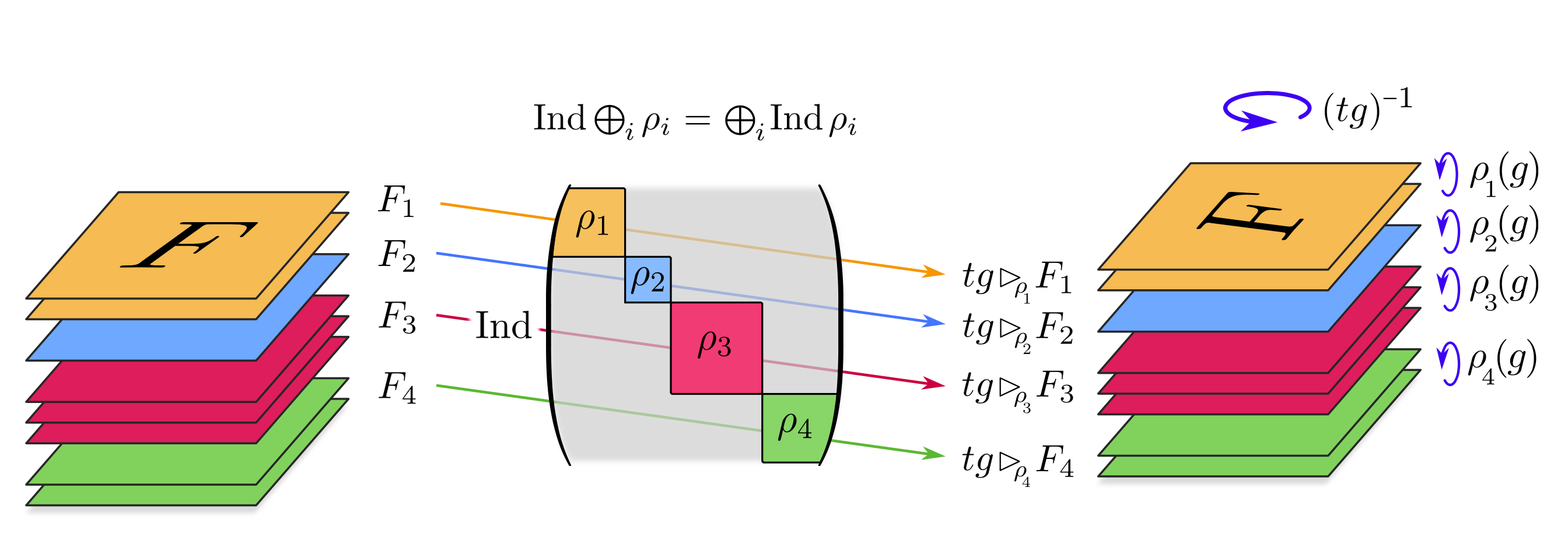
Figure 1. Decomposition of steerable CNNs; [weiler-book, Fig. 4.4]

The goal for the rest of this paper is to develop a similar theory of what is described in this section for artificial neural networks over graded vector spaces or even more generally over graded modules.

4. Graded vector spaces

Here we give the bare minimum of the background graded vector spaces. The interested reader can check details at [bourbaki], [roman], [kocul] among other places.

A graded vector space is a vector space that has the extra structure of a grading or gradation, which is a decomposition of the vector space into a direct sum of vector subspaces, generally indexed by the integers. For the purposes of this paper we will focus on graded vector spaces indexed by integers, but we also give below the definition of such spaces for a general index set $I$.

4.1. Integer gradation

Let $\mathbb{N}$ be the set of non-negative integers. An $\mathbb{N}$–graded vector space, often called simply a graded vector space without the prefix $\mathbb{N}$, is a vector space $V$ together with a decomposition into a direct sum of the form

$${\displaystyle V=\bigoplus_{n\in\mathbb{N}}V_{n}}$$

where each $V_{n}$ is a vector space. For a given $n$ the elements of $V_{n}$ are then called homogeneous elements of degree $n$.

Graded vector spaces are common. For example the set of all polynomials in one or several variables forms a graded vector space, where the homogeneous elements of degree n are exactly the linear combinations of monomials of degree $n$.

Example 4.

Let $k$ be a field and consider $\mathcal{V}_{(2,3)}$ the space of degree 2 and 3 homogenous polynomials in $k[x,y]$. It is decomposed as $\mathcal{V}_{(2,3)}=\mathcal{V}_{2}\oplus\mathcal{V}_{3}$, whwre $\mathcal{V}_{2}$ is the space of binary quadratics and $V_{3}$ the space of binary cubics. Let $\mathbf{u}=[f,g]\in\mathcal{V}_{2}\oplus\mathcal{V}_{3}$. Then the scalar multiplication works as

$$\lambda\star\mathbf{u}=\lambda\star[f,g]=[\lambda^{2}\,f,\lambda^{3}\,g]$$

We will use this example repeatedly for the rest of the paper. ∎

Next we give another example that was our main motivation for machine learning models over graded vector spaces.

Example 5 (Moduli space of genus 2 curves).

Assume $\mbox{char }k\neq 2$ and $C$ a genus 2 curve defined over $k$. Then $C$ has affine equation $y^{2}=f(x)$ where $f(x)$ is a degree 6 polynomial. The ismorphism class of $C$ is determined by its invariants $J_{2},J_{4},J_{6},J_{10}$, which are homogenous polynomials of degree 2, 4, 6, and 10 respectively in terms of the coefficients of $C$. The moduli space of genus 2 curves defined over $k$ is isomorphic to the weighted projective space $\mathbb{WP}_{(2,4,6,10),k}$.

4.2. General gradation

The subspaces of a graded vector space need not be indexed by the set of natural numbers, and may be indexed by the elements of any set $I$. An $I$-graded vector space $V$ is a vector space together with a decomposition into a direct sum of subspaces indexed by elements $i$ of the set $I$:

$${\displaystyle V=\bigoplus_{i\in I}V_{i}}$$

The case where $I$ is the ring $\mathbb{Z}/2\mathbb{Z}$ (the elements 0 and 1) is particularly important in physics. A ($\mathbb{Z}/2\mathbb{Z}$)-graded vector space is known as a supervector space.

4.3. Graded linear maps

For general index sets $I$, a linear map between two $I$-graded vector spaces $f:V\to W$ is called a graded linear map if it preserves the grading of homogeneous elements,

$$f(V_{i})\subseteq W_{i},\quad\text{ for all }\quad i\in I.$$

A graded linear map is also called a homomorphism (or morphism) of graded vector spaces, or homogeneous linear map.

When $I$ is a commutative monoid (such as $\mathbb{N}$), then one may more generally define linear maps that are homogeneous of any degree $i$ in $I$ by the property

$$f(V_{j})\subseteq W_{i+j},\quad\text{for all }\quad j\in I$$

where ”+” denotes the monoid operation. If moreover $I$ satisfies the cancellation property so that it can be embedded into an abelian group $A$ that it generates (for instance the integers if $I$ is the natural numbers), then one may also define linear maps that are homogeneous of degree $i$ in $A$ by the same property (but now ”+” denotes the group operation in $A$). Specifically, for $i\in I$ a linear map will be homogeneous of degree $-i$ if

$$f(V_{i+j})\subseteq W_{j},\;\text{ for all }\;j\in I,\;\text{ while }\;f(V_{j})=0\;\text{ if }\;j-i\notin I$$

Let us see a simple example of a graded linear map.

Example 6.

Consider $\mathcal{V}_{(2,3)}=V_{2}\oplus V_{3}$ as in Example 4. Then a linear map $L:\mathcal{V}_{(2,3)}\to\mathcal{V}_{(2,3)}$ satisfies

$$L([\lambda\star\mathbf{u}])=L([\lambda^{2}f,\lambda^{3}g])=[\lambda^{2}L(f),\lambda^{3}L(g)]=\lambda\star[L(f),L(g)]=\lambda\star L(\mathbf{u})$$

and

$$\begin{split}&L\left([f,g]\oplus[f^{\prime},g^{\prime}]\right)=L\left([f+f^{\prime},g+g^{\prime}]\right)=[L(f)+L(f^{\prime}),L(g)+L(g^{\prime})]\\ &=[L(f),L(g)]\oplus[L(f^{\prime}),L(g^{\prime})]=L([f,g])\oplus L([f^{\prime},g^{\prime}])\end{split}$$

We can see things more explicitly if we choose a basis for $\mathcal{V}_{(2,3)}$. Since $V_{2}$ is the space of binary quadratics $ax^{2}+bxy+cy^{2}$ we can pick the standard basis of monomials for $V_{2}$ as $\mathcal{B}_{1}=\{x^{2},xy,y^{2}\}$. Similarly a standard basis for $V_{3}$ can be chosen as $\mathcal{B}_{2}=\{x^{3},x^{2}y,xy^{2},y^{3}\}$. Hence, a basis for $\mathcal{V}_{(2,3)}$ can be picked as

$$\mathcal{B}=\{x^{2},xy,y^{2},x^{3},x^{2}y,xy^{2},y^{3}\}$$

For example, the polynomial $F(x,y)=\left(x^{2}+xy+y^{2}\right)+\left(x^{3}+x^{2}y+xy^{2}+y^{3}\right)$ has coordinates $\mathbf{u}=[1,1,1,1,1,1,1]^{t}$ in this basis. ∎

Further details on isomorphisms of graded rings of linear transformations of graded vector spaces can be found in [bourbaki], [balaba], [bondarenko], and others.

Notice that the simplest graded linear map is the ”multiplication” by a scalar, say $L(\mathbf{x})=\lambda\mathbf{x}$ which has matrix representation the diagonal matrix

$$\begin{bmatrix}\lambda^{q_{0}}&0&0&\dots\\ 0&\lambda^{q_{1}}&0&\vdots\\ \vdots&0&\ddots&0\\ \dots&\dots&0&\lambda^{q_{n}}\\ \end{bmatrix}$$

4.4. Operations over graded vector spaces

Some operations on vector spaces can be defined for graded vector spaces as well. For example, given two $I$-graded vector spaces $V$ and $W$, their direct sum has underlying vector space $V\oplus W$ with gradation

$$\left(V\oplus W\right)_{i}=V_{i}\oplus W_{i}$$

If $I$ is a semigroup, then the tensor product of two $I$-graded vector spaces $V$ and $W$ is another $I$-graded vector space,

$$\left(V\otimes W\right)_{i}=\bigoplus_{(j,k):j+k=i}(V_{j}\otimes W_{k})$$

We will come back back to tensor products of vectors spaces when more details are needed.

4.5. Inner graded vector spaces

Consider now the case when each $V_{i}$, is a finite fdimensional inner space and let $\langle\cdot,\cdot\rangle_{i}$ denote the corresponding inner product. Then we can define an inner product on $V$ as follows. For $\mathbf{u}=u_{1}+\ldots+u_{n}$ and $\mathbf{v}=v_{1}+\ldots+v_{n}$ we define

$$\langle\mathbf{u},\mathbf{v}\rangle=\langle u_{1},v_{2}\rangle_{1}+\ldots+\langle u_{n},v_{n}\rangle_{n}$$

which is the standart product. Then the Euclidean norm is as expected

$$\|\mathbf{u}\|=\sqrt{u_{1}^{2}+\ldots+u_{n}^{2}}$$

If such $V_{i}$ are not necessary finite dimensional then we have to assume that $V_{i}$ is a Hilbert space (i.e. a real or complex inner product space that is also a complete metric space with respect to the distance function induced by the inner product). This case of Hilbert spaces is especially important in machine learning and artificial intelligence as pointed out by Thm. 5.

Obviously having a norm on a graded vector space is important for machine learning if we want to define a cost function of some type. The simpler case of Euclidean vector spaces and their norms was considered in [moskowitz], [songpon].

Example 7.

Let us continuw with the space $\mathcal{V}_{(2,3)}$ from Example 4. We continue with with bases $\mathcal{B}_{1}=\{x^{2},xy,y^{2}\}$ and $\mathcal{B}_{2}=\{x^{3},x^{2}y,xy^{2},y^{3}\}$ as in Example 6. Hence, a basis for $\mathcal{V}_{(2,3)}$ can be picked as $\mathcal{B}=\{x^{2},xy,y^{2},x^{3},x^{2}y,xy^{2},y^{3}\}$. Let us see how we could define an inner product in $\mathcal{V}_{(2,3)}$. Let $\mathbf{u},\mathbf{v}\in\mathcal{V}_{(2,3)}$ given by

$$\begin{split}\mathbf{u}&=\mathbf{a}+\mathbf{b}=\left(u_{1}\,x^{2}+u_{2}\,xy+u_{3}\,y^{2}\right)+\left(u_{4}\,x^{3}+u_{5}\,x^{2}y+u_{6}\,xy^{2}+u_{7}\,y^{3}\right)\\ \mathbf{v}&=\mathbf{a}^{\prime}+\mathbf{b}^{\prime}=\left(v_{1}\,x^{2}+v_{2}\,xy+v_{3}\,y^{2}\right)+\left(v_{4}\,x^{3}+v_{5}\,x^{2}y+v_{6}\,xy^{2}+v_{7}\,y^{3}\right)\end{split}$$

Then

$$\begin{split}\langle\mathbf{u},\mathbf{v}\rangle&=\langle\mathbf{a}+\mathbf{b},\mathbf{a}^{\prime}+\mathbf{b}^{\prime}\rangle=\langle\mathbf{a}+\mathbf{a}^{\prime}\rangle+\langle\mathbf{b}+\mathbf{b}^{\prime}\rangle\\ &=u_{1}v_{2}+u_{2}v_{2}+u_{3}v_{3}+u_{4}v_{4}+u_{5}v_{5}+u_{6}v_{6}+u_{7}v_{7}\end{split}$$

and the Euclidean norm is defined as expected $\|\mathbf{u}\|=\sqrt{u_{1}^{2}+\ldots u_{7}^{2}}$. ∎

There are other ways to define a norm on graded spaces. Consider a Lie algebra $\mathfrak{g}$. It is called graded if there is a finite family of subspaces $V_{1},\ldots,V_{r}$ such that $\mathfrak{g}=V_{1}\oplus\dots\oplus V_{r}$ and $[V_{i},V_{j}]\subset V_{i+j}$, where $[V_{i},V_{j}]$ is the Lie bracket. When $\mathfrak{g}$ is graded we define for $t\in\mathbb{R}^{\times}$, $\alpha_{t}:\mathfrak{g}\to\mathfrak{g}$ such that

$$\alpha_{t}(v_{1},\ldots,v_{n})=(tv_{1},t^{2}v_{2},\ldots,t^{r}v_{r}).$$

We define a homogenous norm on $\mathfrak{g}$ as

$$\|\mathbf{v}\|=\|(v_{1},\ldots,v_{n})\|=\left(\|v_{1}\|_{1}^{2r}+\|v_{2}\|_{2}^{2r-2}+\dots+\|v_{r}\|_{r}^{2}\right)^{1/2r}$$

where $\|\cdot\|_{i}$ is the Euclidean norm in $V_{i}$. For details see [Moskowitz2, moskowitz]. It is shown in [songpon] that this norm satisfies the triangle inequality.

A more general approach is considered in [SS] defining norms for line bundles and using such norms in the definition of weighted heights on weighted projective variaties.

5. Artificial neural networks over graded vector spaces

Let us now try to design artificial neural networks over graded vector spaces. Let $k$ be a field and for any integer $n\geq 1$ denote by $\mathbb{A}_{k}^{n}$ (resp. ${\mathbb{P}}_{k}^{n}$) the affine (resp. projective) space over $k$. When $k$ is an algebraically closed field, we will drop the subscript. A fixed tuple of positive integers $\mathbf{w}=(q_{0},\dots,q_{n})$ is called set of weights. The weight of $\alpha\in k$ will be denoted by $\mathbf{wt}(\alpha)$. The set

$$\mathcal{V}_{\mathbf{w}}^{n}(k):=\{(x_{1},\ldots,x_{n})\in k^{n}\;|\;\mathbf{wt}(x_{i})=q_{i},\,i=1,\ldots,n\}$$

is a graded vector space over $k$. From now on, when there is no confusion we will simply use $\mathcal{V}_{\mathbf{w}}$ for a graded vector space.

We follow the analogy with the classical case of artificial neural networks. A neuron on a graded vector space $\mathcal{V}_{\mathbf{w}}$ is a function $f:\mathcal{V}_{\mathbf{w}}^{n}\to k$ such that

$$\alpha_{\mathbf{w}}(\mathbf{x})=\sum_{i-0}^{n}w_{i}^{q_{i}}x_{i}+\mathbf{b},$$

where $\mathbf{b}\in k$ is a constant called bias. We can generalize neurons to tuples of neurons via

$$\begin{split}\phi:=\mathcal{V}_{\mathbf{w}}^{n}(k)&\to\mathcal{V}_{\mathbf{w}}^{n}(k)\\ \mathbf{x}&\to g\left(\alpha_{0}(\mathbf{x}),\ldots,\alpha_{n}(\mathbf{x})\right)\end{split}$$

for any gives set of weights $\mathbf{w}_{0},\ldots,\mathbf{w}_{n}$. Then $\phi$ is a $k$-linear function with matrix written as

$$\phi(\mathbf{x})=W\cdot\mathbf{x}+\mathbf{b},$$

for some $\mathbf{b}\in k^{n+1}$ and $W$ an $n\times n$ matrix with integer entries.

Remark 1.

There is a big confusion here when it comes to terminology. The elements $w_{i}$ are called weights in classical neural networks, but these are different from weights of the graded vector space $q_{i}$. The matrix $W$ is called the matrix of weights since it is the matrix $W=[w_{i,j}]$, but again those weights are not the same as weights $q_{0},\ldots,q_{n}$.

A non-linear function $g:\mathcal{V}_{\mathbf{w}}^{n}\to\mathcal{V}_{\mathbf{w}}^{n}$ is called an graded activation function. A graded network layer is a function

$$\begin{split}\mathcal{V}_{\mathbf{w}}^{n}(k)&\to\mathcal{V}_{\mathbf{w}}^{n}(k)\\ \mathbf{x}&\to g\left(W\cdot\mathbf{x}+\mathbf{b}\right)\end{split}$$

for some some activation function $g$. A graded neural network is the composition of many layers. The $l$-th layer

$$\begin{split}\cdots\longrightarrow\mathcal{V}_{\mathbf{w}}^{n}(k)&\stackrel{{\scriptstyle\phi_{l}}}{{\longrightarrow}}\mathcal{V}_{\mathbf{w}}^{n}(k)\longrightarrow\cdots\\ \mathbf{x}&\longrightarrow\phi_{l}(\mathbf{x})=g_{l}\left(W^{l}\mathbf{x}+\mathbf{b}^{l}\right),\end{split}$$

where $g_{l}$, $W^{l}$, and $\mathbf{b}^{l}$ are the activation, matrix, and bias corresponding to this layer. After $m$ layers the output (predicted values) will be denoted by $\hat{\mathbf{y}}=[\hat{y}_{1},\ldots,\hat{y_{n}}]^{t}$, where

$$\hat{\mathbf{y}}=\phi_{m}\left(\phi_{m-1}\left(\ldots(\phi_{1}(\mathbf{x}))\ldots\right)\right),$$

while the true values by $\mathbf{y}=[y_{1},\ldots,y_{n}]^{t}\in\mathcal{V}_{\mathbf{w}}^{n}$.

The relu activation function for graded neural networks can be defined analougusly. Let $\mathbf{x}=[x_{0},\ldots,x_{n}]^{t}\in V_{\mathbf{w}}^{n}$. Then for each coordinate $i=0,\ldots,n$ we define

$$\operatorname{ReLu}_{i}(x_{i})=\max\{0,\left\lvert\mspace{1.0mu}x_{i}\mspace{1.0mu}\right\rvert^{1/q_{i}}\}$$

Hence, is defined as

$$\operatorname{ReLu}(\mathbf{x}):=[\operatorname{ReLu}_{0}(x_{0}),\ldots,\operatorname{ReLu}_{n}(x_{n})]$$

Example 8.

Consider $\mathcal{V}_{(2,3)}$ as above. Let $\mathbf{u}\in\mathcal{V}_{(2,3)}$. Then, $\mathbf{u}=f+g$ such that $f\in V_{2}$ and $g\in V_{3}$. Assume

$$f=2x^{2}-9xy+y^{2},\qquad\text{ and }\qquad g=x^{3}-2x^{2}y+xy^{2}+y^{3}$$

The coordinated of $\mathbf{u}$ with respect to the basis $\mathcal{B}$ fixed in Example 4 are $\mathbf{u}_{\mathcal{B}}=[2,-3,1,1,-2,11]^{t}$ and

$$\operatorname{ReLu}(\mathbf{u})=[\sqrt{2},3,1,1,\sqrt{2},1,1]^{t}.$$

It remains to be seen if this activation function or many others which can be adopted in our settings will be efficient. Notice the similarity of this definition with the weighted heights defined in [SS, vojta].

5.1. Artificial neural networks on weighted projective spaces

Our intention is to build a complete theory of equivariant nueral networks over graded vector spaces and make it possible to design machine learning models to study weighted projective spaces and weighted varieties among other applications. It is unclear how such models would perform, however mathematically there is every reason to believe that computations on weighted projective varieties are more efficient than over classical projective varieties.

In [sh-2024] we used current techniques of machine learning to study the weighted projective space $\mathbb{WP}_{(2,4,6,10)}$ which is the moduli soace of genus two curves. The input features were invariants $J_{2},J_{4},J_{6}$, and $J_{10}$, which represent a point in a graded space. However, current techniques are designed for classical vector spaces. Hence, while we got some interesting results in [sh-2024] we weren’t sure what these results represent. In other words, one can’t really understand what is happening in a graded space unless the gradation becomes part of the training.

This paper is the first attempt in what we envision as a long project of machine learning in graded vector spaces. Most of mathematical details have yet to be worked out and one has to explore graded Lie algebras, graded manifolds and also different gradings. Especially interesting is the case when the ground field is not $\mathbb{R}$ or $\mathbb{C}$, but $\mathbb{Q}$ or a a field of positive characteristic. Such tasks present challenges mathematically and from the implementation point of view and their performance and efficiency are still open questions.