Quantifying energy fluence and its uncertainty for radio emission from particle cascades in the presence of noise

Abstract

Measurements of radio signals induced by an astroparticle generating a cascade present a challenge because they are always superposed with an irreducible noise contribution. Quantifying these signals constitutes a non-trivial task, especially at low signal-to-noise ratios (SNR). Because of the randomness of the noise phase, the measurements can be either a constructive or a destructive superposition of signal and noise. To recover the electromagnetic energy of the cascade from the radio measurements, the energy fluence, i.e. the time integral of the Poynting vector, has to be estimated. Conventionally, noise subtraction in the time domain has been employed for energy fluence reconstruction, yielding significant biases, including even non-physical and negative values. To mitigate the effect of this bias, usually an SNR threshold cut is imposed, at the expense of excluding valuable data from the analyses. Additionally, the uncertainties derived from the conventional method are underestimated, even for large SNR values. This work tackles these challenges by detailing a method to correctly estimate the uncertainties and lower the reconstruction bias in quantifying radio signals, thereby, ideally, eliminating the need for an SNR cut. The development of the method is based on a robust theoretical and statistical background, and the estimation of the fluence is performed in the frequency domain, allowing for the improvement of further analyses by providing access to frequency-dependent fluence estimation.

1 Introduction

Radio detection can be employed to measure cosmic-rays, photons, and neutrinos generating extensive air showers and particle cascades in dense media Huege [10]Schröder [23]. Since the radio emission is proportional to the number of electrons and positrons in the cascade, by quantifying the underlying signal of a measured radio pulse we can access the electromagnetic component of a shower, and, thus, estimate the electromagnetic energy of the originating particle. Since the electromagnetic energy is proportional to the area integral of the energy fluence (the energy deposit per unit area in terms of radio waves)[2], a correct reconstruction of the electromagnetic energy and its uncertainty relies on the determination of the energy fluence and its uncertainty. The total energy fluence $f_{\mathrm{tot}}$ at a given antenna position is the time integral of the Poynting vector. For discretely sampled measurements, this means:

$$f_{\mathrm{tot}}=\epsilon_{0}\,c\,\Delta t\sum_{\mathrm{pol}}\bigg{(}\sum_{j}E^{2}_{\mathrm{pol}}(t_{j})\bigg{)},$$ (1)

where $\Delta t$ is the sampling interval of $\vec{E}(t)$, the observed three-dimensional electric-field vector (in the equation broken down into its components), $\epsilon_{0}$ is the vacuum permittivity, and $c$ is the speed of light. Note that the evaluation of eqn.1 does not depend on the choice of the coordinates system into which $\vec{E}(t)$ is decomposed. In an analogous way, we can express the energy fluence as the sum of component-dependent contributions $f_{\mathrm{pol}}$:

$$f_{\mathrm{pol}}=\epsilon_{0}\,c\,\Delta t\sum_{j}E^{2}_{\mathrm{pol}}(t_{j})\,\,\rightarrow\,\,f_{\mathrm{tot}}=\sum_{\mathrm{pol}}f_{\mathrm{pol}}.$$ (2)

Unlike other measurements in the field of particle physics, where the noise consistently adds up with the signal and can easily be subtracted from the latter, radio measurements require a more sophisticated treatment of the noise. The measured radio pulse is either enhanced or diminished compared to the true signal depending on the phase of the radio noise. In other words, since the phase of the radio noise is randomly distributed, the signal and the noise can add up constructively or destructively. This makes the evaluation of the fluence in the presence of noise non-trivial, especially at low signal-to-noise ratios (SNR)[22].

So far, the conventional way of reconstructing the signal energy fluence consisted of estimating and subtracting the noise fluence in the time domain [6], as described in sec. 3. For the reasons mentioned above, this way of treating the noise leads to a non-negligible reconstruction bias at low SNR values, as discussed in sec. 5. In particular, by subtracting the noise, the fluence estimators can assume negative non-physical values. To avoid the introduction of a large bias, especially in the reconstruction of the electromagnetic energy, a minimum required SNR value is typically introduced to use data from a given antenna. This is the approach used so far in the context of several radio-related experiments, such as the Pierre Auger Observatory[1] and LOFAR[5], where a cut at the level of the electric field for a given antenna station is applied. One of the aims of this work is to mitigate the reconstruction bias allowing the lowering and, ideally, removal of the need for an SNR cut. In this way, the information contained in the measurements of those antennas previously excluded can be exploited in further analysis. Furthermore, the uncertainties derived from the noise-subtraction method turn out to be underestimated, as we will show in sec. 5.

In this work, we detail a method for the quantification of the energy fluence and its uncertainty, exploiting a solid statistical background based on Rice distributions, as described in sec. 4.2. The same statistical background has already been used within the ANITA experiment to achieve an estimation of the fluence in the frequency domain by employing fitting procedures[21]. Our method is based on the estimation of the fluence in the frequency domain, too, i.e., provides access to a frequency-dependent fluence estimation. Since the spectral shape can be described more easily than the pulse shape in the time domain, the method presented here can be further developed by combining it with the information derived from spectral modeling [13]. In the following, we validate the Rice-distribution method and compare it to the so-far widely adopted noise subtraction method. The bias of the reconstructed fluence as a function of the SNR will be discussed, as well as the evaluation of the uncertainties.

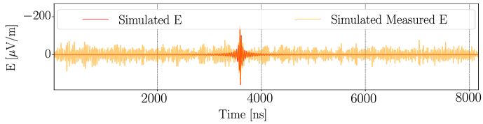
Figure 1: Example of an electric-field component simulated in the absence of noise (red) and in the presence of noise (orange).

For the validation and comparison, both methods are applied to the same data set of simulated air showers initiated by cosmic-rays. Because of its complexity, it is a non-trivial task to artificially generate realistic noise. Apart from electronics noise, the ambient radio background contains diffusive galactic emission and human-made radio-frequency interference. To realistically simulate radio measurements, we have added the ambient background recorded at a particular site of the Pierre Auger Observatory to the radio-emission simulations, as explained in sec. 2. Even though the background is not representative of the entire array, nor other experiment locations, by using these measurements we get a realistic SNR distribution. Furthermore, we simulate the antenna response of the Radio Detector (RD)[11] of the Pierre Auger Observatory, sensitive to the 30-80 MHz frequency bandwidth with $\overline{\mathrm{Off}}\underline{\mathrm{line}}$[3], the framework of the Pierre Auger collaboration. Nevertheless, the results of our study are independent of the detector simulation, as explained in sec. 2, and the Rice-distribution method can be applied to larger frequency bandwidths than the one tested in this work.

In the Appendix B, we also present a method for estimating the spectral amplitudes of the signal and their uncertainties based on maximizing the Rice likelihood function. It is worth mentioning that the method can be employed in the time domain, too, and be further developed. In the Appendix C, the reader can find tables listing most of the notation and variables adopted in the following.

2 Simulated Data Set

Here, we shortly describe the set of simulations used.

2.1 Particle Simulations and Simulated Radio-footprints

To study the performance of the energy fluence estimation methods, we exploit the same set of simulated air showers as used in reference [20]. The showers are initiated by four different cosmic-ray primaries: proton, helium, nitrogen, and iron. For each primary, the particle and radio-emission footprints of about 2000 showers are simulated with CORSIKA/CoREAS v7.7401 [12][9], using the high energy interaction model QGSJETII-04 [18] and an optimized thinning level of $10^{-6}$ [14]. The primaries have energies in the interval between $10^{18.4}$ eV and $10^{20.1}$ eV, while the arrival directions of the showers are uniformly distributed across zenith angles between $65^{\circ}$ and $85^{\circ}$. The environmental conditions are set to match the Pierre Auger Observatory site, as is the detector layout. The cores of the showers are randomly distributed within this detector layout.

2.2 Simulations of Electric Fields in the Absence of Noise

The CoREAS simulations are processed through the reconstruction framework $\overline{\mathrm{Off}}\underline{\mathrm{line}}$. The RD response simulation is performed and the electric field traces are reconstructed from the raw signal traces by using the Monte Carlo values of the arrival direction and the sensitivity pattern of the RD antennas. This means that the antenna response is applied to the CoREAS radio pulses and then again deconvolved. The electric field traces obtained correspond to the air shower pulses as they would be reconstructed in the absence of noise, in the 30-80 MHz frequency band. Each trace has a length of 8192 ns and $\Delta t$=1 ns, upsampled from the nominal 250 MSPS sampling rate with a factor of four. These traces are used in sec. 5 to evaluate the reference values of the energy fluence to be compared to the fluence estimators obtained in the presence of noise. In this way, the analysis is not affected by biases potentially introduced by the unfolding of the antenna response.

2.3 Simulations of Measured Electric Fields in the Presence of Noise

To get the simulated measurements of the cosmic-ray pulses in the presence of noise, we apply the detector simulation to the CoREAS simulations and add measured noise data. The measured traces of the ambient background recorded at the Pierre Auger Observatory site operating over one year are added to the digitized simulated traces. Each noise measurement is used multiple times by rolling the trace. The resulting traces are used in sec. 5 to evaluate the energy fluence estimators in the presence of noise. In figure 1, we show an example of a simulated trace in the absence of noise and the corresponding trace simulated in the presence of noise, obtained as just described.

3 The Noise Subtraction Method

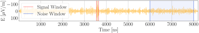
Figure 2: Signal window (between red lines) and noise window (between blue lines) as used in the noise subtraction method.

The noise subtraction method, adopted by many experiments so far, is based on the assumption that the measured amplitude of the electric field is given by the sum of the cosmic-ray radio pulse and Gaussian-distributed noise $e(t)$, having a certain standard deviation $\sigma_{e}$ and centered on zero [6]. To estimate the energy fluence, we define a noise window, delimited by $t_{1}$ and $t_{2}$, and a signal window, delimited by $t_{3}=t_{\mathrm{peak}}-\Delta$ and $t_{4}=t_{\mathrm{peak}}+\Delta$, where $t_{\mathrm{peak}}$ indicates the position of the radio pulse in the time trace, and $\Delta$ has to be chosen such as to contain most of the pulse. As shown in figure 2, the noise window has to be far away from the signal window to contain mainly only noise contribution. For each component of the measured electric field at a given antenna position $E_{\mathrm{pol}}(t)$, the energy fluence is estimated as:

$$\hat{f}_{\mathrm{pol}}=\epsilon_{0}\,c\,\Delta t\bigg{(}\sum_{t_{j}=t_{3}}^{t_{4}}E_{\mathrm{pol}}^{2}(t_{j})-\frac{t_{4}-t_{3}}{t_{2}-t_{1}}\sum_{t_{j}=t_{1}}^{t_{2}}E_{\mathrm{pol}}^{2}(t_{j})\bigg{)},$$ (3)

where the normalized fluence in the noise window is subtracted from the fluence calculated in the signal window. The uncertainty on the fluence estimator, as derived in [6], consists of:

$$\delta\big{(}\hat{f}_{\mathrm{pol}}\big{)}=\sqrt{4\,\epsilon_{0}\,c\,\Delta t\,\hat{f}_{\mathrm{pol}}\,\sigma_{e}^{2}\,+\,2\,(\epsilon_{0}\,c)^{2}\,\Delta t\,\sigma_{e}^{4}},$$ (4)

where $\sigma_{e}$ can be approximated with the RMS of the trace computed in the noise window. The estimator of the total energy fluence at the antenna position is given by the sum of the estimators over the polarisations, as $\hat{f}_{\mathrm{tot}}=\sum_{\mathrm{pol}}\hat{f}_{\mathrm{pol}}$. We evaluate its uncertainty by propagating the errors $\delta\big{(}\hat{f}_{\mathrm{pol}}\big{)}$ over the polarisations.

4 Rice-distribution Method

Unlike the relatively straightforward noise subtraction method, the Rice-distribution method comprises several steps. Here, we summarize the general logic behind the method, with detailed explanations and discussion provided in the subsequent sections.

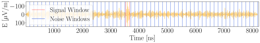
Figure 3: Signal window (between red lines) and noise windows (between blue lines) as used in the Rice-distribution method. In the example, $N$=57 noise windows are used.

For each component of the measured electric field at a given antenna position, we define a signal window and $N$ noise windows along the time trace, as shown in the example of figure 3. Since our method relies on estimating the energy fluence in the frequency domain, we ensure a correct and efficient evaluation by applying further processing of the windows: before and after performing any Fourier transform, we employ, respectively, windowing and filtering (sec. 4.1). This results in a signal-window frequency spectrum of $M$ Rice-distributed spectral amplitudes, and $N$ noise frequency spectra, each having $M$ spectral amplitudes assumed to be Rayleigh-distributed (sec. 4.2). We express the measured fluence as the sum of $M$ frequency-dependent contributions. For each frequency, we estimate the noise fluence over the $N$ windows and, finally, estimate the signal fluence and its uncertainty. A summary of the formulas used is provided in section 4.3, while the derivation of these formulas - obtained by exploiting the statistical background based on the Rice distribution - can be found in Appendix A. In sec. 4.4, we study the bias of the signal fluence estimator and the coverage of its error by performing a toy Monte Carlo for a single frequency. Finally, by summing up the $M$ signal estimators and propagating the errors, we obtain the estimator of the polarization fluence and its uncertainty. The logic is illustrated in the flowchart of figure 4.

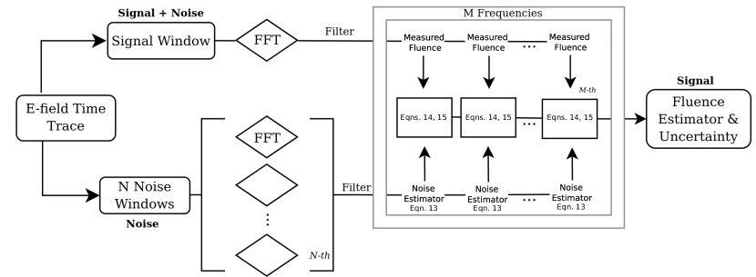
Figure 4: Flowchart representing the logic of the energy fluence estimation for a single polarisation of the electric field. Combining the $M$ estimators of the noise fluence obtained from the $N$ noise windows, and the fluence measured in the signal window, we get the polarisation fluence estimator and its uncertainty.

To finally estimate the total fluence at the antenna position and its uncertainty, we repeat this process for the remaining polarizations.

4.1 Signal and Noise Windows

As anticipated, in our method we define a signal window and $N$ noise windows along the time trace of the measured electric-field component. To be able to estimate the fluence in the frequency domain, we need to compute the discrete Fourier transform (DFT) over the windows. Specifically, we employ a fast Fourier transform (FFT) algorithm.

When calculating a DFT, we implicitly assume that the finite sequence of considered samples is periodic in time. If the start and end points of the sequence are not matching each other, artificial spectral contributions are introduced in the frequency spectrum. To reduce the spectral leakage, it is recommended to apply a tapering function[8]. In the implementation of our method, anytime we perform an FFT of a sequence of samples, we apply in the time domain the so-called Tukey window[24]. This is a symmetrical function consisting of a rectangular function combined with two halves of a Hann window, also known as raised cosine bell window[8]. For this reason, the Tukey window is often referred to as split cosine bell or cosine-tapered window. Given a Tukey window of total length $L_{\mathrm{tot}}=N_{\mathrm{tot}}\Delta\,t$, where $N_{\mathrm{tot}}$ is the total number of the samples of the considered sequence, one can require the proportion $p$ of the sequence to be tapered by the two halves of the Hann window. In other words:

$$L_{\mathrm{H}}=p\,L_{\mathrm{tot}}=N_{\mathrm{H}}\,\Delta t,\quad\mathrm{with}\,\,\,\,N_{\mathrm{H}}=p\,N_{\mathrm{tot}},$$ (5)

where $L_{\mathrm{H}}$ is the length of the Hann window and $N_{\mathrm{H}}$ is the total number of samples covered by its two halves.

To properly define the signal window, we employ the Tukey window just introduced. First, we fix $L_{\mathrm{tot}}=140$ ns, and $L_{\mathrm{H}}=40$ ns, then, we clip the time trace around the pulse position $t_{\mathrm{peak}}$ such that the resulting clipped trace has a length equal to $L_{\mathrm{tot}}$. Finally, we apply the Tukey window and we perform the FFT of the windowed trace. Because of the usage of windowing, the resulting spectrum could present a non-negligible contribution outside the sensitive frequency bandwidth of interest. For this reason, these spectral amplitudes are filtered out. To evaluate the noise level of the measurement, we now define $N$ noise windows. Starting from the beginning of the trace, we apply the Tukey window every multiple of $L_{\mathrm{tot}}$, until we cover the entire trace length. We take care of skipping the signal window and applying an additional spacing to reduce the signal contribution to the noise evaluation. In this work, we use a spacing of $\pm$20 ns and the same $L_{\mathrm{tot}}$ and $L_{\mathrm{H}}$ employed for the signal window. This results in having about $N\approx 60$ noise windows per measured trace. After performing the FFT in each window, we filter the spectra obtaining the same number of spectral amplitudes as achieved from the signal window. In figure 5, we show the frequency spectra obtained from the signal window and one of the neighboring noise windows, after applying the Tukey function to a time trace of our data set. Note that by filtering the frequencies outside the 30-80 MHz bandwidth, we get M=7 spectral amplitudes.

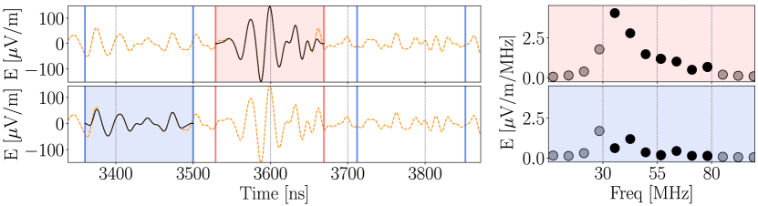
Figure 5: Examples of signal window (upper plots) and noise window (lower plots) as defined for the Rice-distribution method. On the left, we show the time trace before (orange) and after (black) applying the Tukey function in the signal window (red) and the noise window (blue). On the right, the corresponding frequency spectra are shown using the same color code, with the black dots indicating the spectral amplitude obtained after filtering in the 30-80 MHz frequency band.

4.2 Rice Distribution

After defining the signal window and performing the FFT, we obtain $M$ measured spectral amplitudes $a(\nu_{j})$, where the index $j$ runs over $M$. These amplitudes are given by the superposition of the true signal and the measurement noise of each frequency bin. Since radio measurements have both an amplitude and a phase, to recover the unknown spectral amplitudes of the true signal $s(\nu_{j})$, we need to use a formalism that allows us to properly disentangle the phase information from the amplitude. To do this, the phasors’ formalism can be adopted.

Let us first focus on a single-frequency bin, where $\vec{s}$ is a constant phasor representing the true signal, and $\vec{m}=a\,e^{i\theta}$ is the measurement phasor, having amplitude $a$ and phase $\theta$. Following the derivation of reference[7], we express the noise contribution to the measurement as the sum of $\mathcal{N}$ random distributed phasors. The random phasors represent the elementary and monochromatic disturbances to the true signal we aim to estimate. Since many noise sources can contribute to the disturbances (e.g. narrow-band TV transmitters, electronics noise, atmospheric disturbances, broadband galactic background, and so on), it is reasonable to assume $\mathcal{N}$ to be large. We make further assumptions on the noise phasors. We assume that the amplitude and phase characterizing them are statistically independent. Furthermore, we assume that their amplitudes are identically distributed and that their phases are uniformly distributed between $[-\pi,\pi)$. According to these conditions, it can be demonstrated that the marginal probability function (PDF) of the length of the resultant phasor $\vec{n}$, given by the noise random phasors’ sum, is Rayleigh distributed. According to [7], we can express our measurement $\vec{m}$ as the sum of $\vec{s}$ and $\vec{n}$ (as depicted in figure 6), whose amplitude $a$ follows the Rice distribution. In other words, the marginal PDF of $a$ is given by :

$$\mathcal{R}ice(s,\sigma)=\begin{cases}\,\frac{a}{\sigma^{2}}\cdot\mathrm{exp}\left(-\frac{a^{2}+s^{2}}{2\sigma^{2}}\right)\cdot I_{0}\left(\frac{as}{\sigma^{2}}\right)&\text{a $>$ 0}\\ \,0&\text{otherwise},\\ \end{cases}$$ (6)

where $s$ is the amplitude of the signal, $\sigma$ is the scale parameter of the function and represents the noise level of the measurement, and $I_{0}$ is the modified Bessel function of the first kind and order zero. As shown in figure 6, when the signal is large compared to the noise, the Rice distribution can be approximated with a normal distribution having standard deviation equal to $\sigma$ and centered on $\sqrt{s^{2}+\sigma^{2}}$. For low signals, the Rice distribution approaches a Rayleigh distribution.

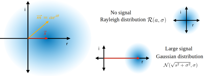
Figure 6: Representation of radio measurements using the phasors’ formalism. In the images, the signal phasor $\vec{s}$ is depicted on the real axis (red). The measurement $\vec{m}$ (orange) is given by the sum of $\vec{s}$ and the sum of the $\mathcal{N}$ random noise phasors. The probability density function of the noise phasor is illustrated as a blue cloud.

In our case, the $M$ measured spectral amplitudes will follow different Rice distributions depending on the unknown underlying signal and noise level of the corresponding frequency bin. Note that the described formalism is valid both in the time and frequency domains, thus the development of further applications is possible in both domains. We refer the reader to Appendix B if interested in the method we have developed to estimate the amplitudes $s(\nu_{j})$ and their errors based on maximizing the Rice likelihood function. In Appendix B, we also describe how to estimate the noise level of the bin over the $N$ noise windows defined in the previous section. In the following, instead, we will summarize the formulas needed to estimate the signal energy fluence and its error in the frequency domain, which remains the main goal of this work. The formulas were obtained starting from the statistical background based on the Rice distribution just described. For a detailed derivation of the formulas, the reader is referred to Appendix A.

4.3 Energy Fluence Estimator and its Uncertainty

To evaluate the energy fluence contained in an electric field component in the frequency domain, we recall Parseval’s theorem:

$$f_{\mathrm{pol}}=\epsilon_{0}\,c\,\Delta t\sum_{j=0}^{N-1}E^{2}_{\mathrm{pol}}(t_{j})=2\,\epsilon_{0}\,c\,\frac{\Delta t}{N}\sum_{j=0}^{M-1}|D_{\mathrm{pol}}(v_{j})|^{2},$$ (7)

where N is the number of samples considered belonging to the time trace, $D_{\mathrm{pol}}$ are the corresponding complex-valued DFTs, and M=$\frac{N}{2}$ is the number of positively valued frequencies. Given the time sample size $\Delta t=\frac{1}{N\Delta\nu}$, where $\Delta\nu$ is the frequency sample size, we can express eqn. 7 as:

$$f_{\mathrm{pol}}=2\,\epsilon_{0}\,c\,\Delta\nu\,\Delta t^{2}\sum_{j=0}^{M-1}|D_{\mathrm{pol}}(v_{j})|^{2}.$$ (8)

Note that the normalization used above considers any change in the number of frequency bins, e.g., in the case of zero padding, and preserves the energy conservation of the integral. Using a different notation, eqn. 8 can be expressed as a sum of the fluences for each frequency:

$$f(\nu_{j})=K\,|D_{\mathrm{pol}}(v_{j})|^{2}\,\,\rightarrow\,\,f_{\mathrm{pol}}=\sum_{j=0}^{M-1}f(\nu_{j}),$$ (9)

where $K=2\,\epsilon_{0}\,c\,\Delta\nu\,\Delta t^{2}$. Let us now consider the ideal case of a signal in the complete absence of noise. According to the notation and formalism introduced in the previous section, and recalling eqn.9, the energy fluence of the unknown signal in the frequency domain can be expressed as:

$$f_{\mathrm{s}}=K\sum_{j=0}^{M-1}s^{2}(v_{j})=\sum_{j=0}^{M-1}f_{\mathrm{s}}(\nu_{j}).$$ (10)

Thus, the estimator of the polarisation fluence and the estimator of the total fluence at the antenna position will be of the form:

$$\hat{f}_{\mathrm{pol}}=\sum_{j=0}^{M-1}\hat{f}_{\mathrm{s}}(\nu_{j})\,\,\rightarrow\,\,\hat{f}_{\mathrm{tot}}=\sum_{\mathrm{pol}}\hat{f}_{\mathrm{pol}},$$ (11)

where $\hat{f}_{\mathrm{s}}(\nu_{j})$ are the signal fluence estimators in the j-th frequency. The fluence of the same signal measured in the presence of random noise will be:

$$\hat{f}_{\mathrm{a}}=K\sum_{j=0}^{M-1}a^{2}(v_{j})=\sum_{j=0}^{M-1}\hat{f}_{\mathrm{a}}(\nu_{j}),$$ (12)

with $a(v_{j})$ being the random spectral amplitudes measured in the signal window, and $\hat{f}_{\mathrm{a}}(\nu_{j})$ representing the frequency-dependent contributions to the amplitude fluence measured in the same window.

For simplicity, let us analyze a single-frequency bin. We estimate the noise fluence of the j-th frequency by exploiting the $N$ noise windows defined in sec. 4.1:

$$\hat{f}_{\mathrm{n}}(\nu_{j})=\frac{K}{N}\sum_{i=0}^{N-1}n_{i}^{2}(v_{j}),$$ (13)

where $n_{i}(v_{j})$ indicates the Rayleigh-distributed random noise of the j-th bin measured in the i-th noise window. In eqn.13, we use the sample mean over the windows, but depending on the characteristic noise of the measurements, one could consider using the sample median value or excluding some of the noise windows from the evaluation. Finally, we define the fluence estimator of the signal in the j-th frequency by subtracting the noise fluence from the amplitude fluence estimators:

$$\hat{f}_{\mathrm{s}}(\nu_{j})=\begin{cases}\hat{f}_{\mathrm{a}}(\nu_{j})-\hat{f}_{\mathrm{n}}(\nu_{j})&\text{$\hat{f}_{\mathrm{a}}(\nu_{j})\geq\hat{f}_{\mathrm{n}}(\nu_{j})$}\\ \,0&\text{$\hat{f}_{\mathrm{a}}(\nu_{j})<\hat{f}_{\mathrm{n}}(\nu_{j})$}.\\ \end{cases}$$ (14)

The intrinsic bias of the estimator of eqn.14 is discussed in sec. 4.4. There, the coverage of its error is studied, too. According to the derivation of Appendix A, the statistical uncertainty can be estimated as:

$$\delta(\hat{f}_{\mathrm{s}}(\nu_{j}))=\sqrt{\hat{f}_{\mathrm{n}}(\nu_{j})\,\big{(}\hat{f}_{\mathrm{n}}(\nu_{j})\,+2\,\hat{f}_{\mathrm{s}}(\nu_{j})\big{)}}$$ (15)

Finally, the fluence estimator of the polarisation and the total fluence estimator can be calculated as in eqns.10. From eqn. 15, we can derive by error propagation their uncertainties.

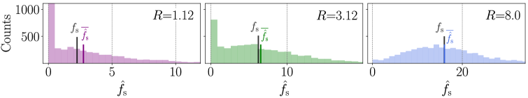
Figure 7: Histograms of the signal fluence estimators obtained by running a toy Monte Carlo for three fixed values of $R$. The vertical black lines indicate the underlying true signal fluence used in the toy Monte Carlo. For comparison, the mean values of the histograms are shown through the colored vertical lines.

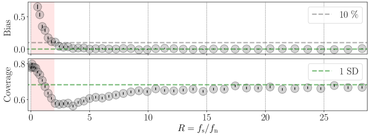
Figure 8: Intrinsic bias of the signal fluence estimator (top) and errors coverage (bottom) obtained by running a toy Monte Carlo for several values of $R$. The orange shadowed area indicates the $R$ range which is strongly biased. In both plots, the error bars are divided by $\sqrt{N_{\mathrm{bin}}}$, with $N_{\mathrm{bin}}$ being the number of entries in the bin.

4.4 Toy Monte Carlo: Bias and Error Coverage for Single-frequency Estimator

In eqn.14, we included the second condition to prevent the signal estimator of a frequency bin from assuming negative unphysical values. This would happen anytime the noise fluence of the bin is larger than the fluence measured in the signal window. However, including this condition introduces a bias, that we evaluated with a toy Monte Carlo. Exploiting the fact that the random variables $a$ are Rice-distributed, according to eqn.6, we generate $N_{\mathrm{MC}}$=5,000 random variables by setting $s$, and thus $f_{\mathrm{s}}$, to fixed values. Without loss of generality, we keep $\sigma$=1 for simplicity and we define the noise parameter $f_{\mathrm{n}}:=2\,\sigma^{2}$. For each amplitude $a$, we evaluate the noise fluence estimator $\hat{f}_{\mathrm{n}}$ as the mean over $N$ random variables following a normal distribution having mean $\mu=2\,\sigma^{2}$ and variance Var=4 $\sigma^{4}/N$, where $N$ is the number of noise windows used in this work (see Appendix A for a detailed explanation). Finally, we evaluate the signal fluence estimator $\hat{f}_{\mathrm{s}}$ and its uncertainty according to eqns.14 and 15. In figure 7, we show some examples of estimator distributions generated with the toy Monte Carlo for three fixed values of $R=1.12,3.12,8.0$, the signal-to-noise ratio of the frequency bin given by $R=f_{\mathrm{s}}/f_{\mathrm{n}}$. In the histograms relative to $R=1.12,3.12$, the presence of a peak in correspondence of the bin including the estimators $\hat{f}_{\mathrm{s}}=0$ can be noticed. On the contrary, in the histogram relative to $R=8.0$, the number of entries in the same bin decreases significantly. As anticipated, this reflects a bias that gets less prominent with increasing values of $R$. We tackled the dependence on $R$ by scanning several values and computing the relative bias and its standard deviation as:

$$\psi=\overline{\hat{f}_{\mathrm{s}}}/f_{\mathrm{s}}-1,\,\,\,\sigma_{\psi}=\sqrt{\sum_{i=0}^{N_{\mathrm{MC}}-1}\frac{(\hat{f}_{\mathrm{s},i}-\overline{\hat{f}_{\mathrm{s}}})^{2}}{N_{\mathrm{MC}}-1}},$$ (16)

where $\overline{\hat{f}_{\mathrm{s}}}$ is the mean value of the estimators obtained through the toy Monte Carlo. Finally, we express the bias as a function of $R$. As shown in the upper plot of figure 8, the relative bias is larger than 10% up to $R=$2. For higher values of $R$, the bias decreases and can be neglected. According to the definition of SNR adopted (see sec. 5.1) and the data set employed to validate our method in sec. 5.2, the intrinsic bias seems to affect the bias of the polarisation estimator mostly up to SNR${}_{\mathrm{pol}}\approx 1.6$. We studied also the coverage of the errors as a function of $R$. We define the coverage as the percentage of data satisfying the condition:

$$f_{\mathrm{s}}\in[\hat{f}_{\mathrm{s}}-\delta(\hat{f}_{\mathrm{s}}),\hat{f}_{\mathrm{s}}+\delta(\hat{f}_{\mathrm{s}})].$$ (17)

As shown in the lower plot of figure 8, the error coverage depends also on the bias of the estimator. For large bias, we overestimate the errors, while for $R>$2 the coverage approaches the classical definition of standard deviation.

5 Validation of the Method

In this section, we validate the Rice-distribution method and compare it to the noise subtraction method. We apply both methods to electric field traces in the presence of noise, simulated as described in sec. 2.3. In the analysis, no further signal cleaning nor RFI suppression is performed. We study the bias of the fluence estimators derived from the same electric fields in the absence of noise, simulated as explained in sec. 2.2. The coverage of the errors is investigated, too. Both the bias and the uncertainty coverage of the two methods are expressed as a function of the SNR. The SNR definition adopted in the following is described in sec. 5.1.

Since the two methods are different from each other, it is not possible to perform a direct comparison. For this reason, we evaluate the reference values separately for each method. Concerning the noise subtraction method, the reference values are achieved by evaluating eqn. 2 in the signal window defined in sec. 3. For the Rice-distribution method, eqn. 9 is evaluated over the frequency spectrum obtained after applying the signal window defined in sec. 4.1.

We restrict the following analysis to those noisy pulses whose position is known with an accuracy smaller than 2 ns. A further cut on the antenna position is made, to exclude simulated traces strongly affected by thinning artifacts. Thinning manifests itself as after-pulse noise, and it is expected that the artificial power introduced becomes relevant for large distances to the shower axis, where the coherent signal is weak. Following [19], we exclude from further analyses the antenna positions $r/r_{\mathrm{che}}>2$, where $r$ is the distance of the antenna to the shower axis and $r_{\mathrm{che}}$ the Cherenkov radius of the radio-emission footprint.

In sec. 5.2, we compare the goodness of the two methods by analyzing the energy fluence contained in a single polarisation. We break down the electric fields into their East-West (EW), North-South (NS), and Vertical (V) components . To investigate the performance of the two methods, we first study the SNR region we know to be most challenging, i.e. at SNR values below 20, and then we focus on high SNR values. In the next section 5.3, the estimation of total fluence at the antenna position is investigated instead.

5.1 SNR Definition

In the following, we adopt a definition of SNR commonly employed in several radio experiments. We assume that the position of the radio pulse in the trace $t_{\mathrm{peak}}$ is approximately known. Exploiting all the polarisations of the electric field measured at a given antenna position, we define the trace $A_{\mathrm{tot}}^{\mathrm{Hilb}}(t)$ as follows:

$$A_{\mathrm{tot}}^{\mathrm{Hilb}}(t)=\sqrt{\sum_{\mathrm{pol}}\big{|}E_{\mathrm{pol}}^{\mathrm{Hilb}}(t)\big{|}^{2}},$$ (18)

with $E_{\mathrm{pol}}^{\mathrm{Hilb}}(t)$ being the Hilbert envelope of a single component of the electric field. We refer to the amplitude of the trace defined in eqn.18 corresponding to the position $t_{\mathrm{peak}}$ as $A_{\mathrm{tot}}^{\mathrm{Hilb}}|_{\mathrm{max}}$. Far away from $t_{\mathrm{peak}}$, we define a portion of the trace between $t_{1}$ and $t_{2}$, where we calculate the noise level as the root-mean-square (RMS) over the $N$ samples considered:

$$A_{\mathrm{tot}}^{\mathrm{RMS}}=\sqrt{\sum_{\mathrm{t_{j}=t_{1}}}^{t_{2}}\frac{1}{N}\bigg{(}A_{\mathrm{tot}}^{\mathrm{Hilb}}(t_{j})\bigg{)}^{2}}.$$ (19)

Finally, we define $\mathrm{SNR}_{\mathrm{tot}}$, the signal-to-noise ratio over all the polarisations, as:

$$\mathrm{SNR}_{\mathrm{tot}}=\bigg{(}\frac{A_{\mathrm{tot}}^{\mathrm{Hilb}}|_{\mathrm{max}}}{A_{\mathrm{tot}}^{\mathrm{RMS}}}\bigg{)}^{2}.$$ (20)

A similar definition is adopted for a single polarisation. Once the noise level between $t_{1}$ and $t_{2}$ over the $N$ samples of the Hilbert envelope of the component has been calculated as:

$$A_{\mathrm{pol}}^{\mathrm{RMS}}=\sqrt{\sum_{\mathrm{t_{j}=t_{1}}}^{t_{2}}\frac{1}{N}\bigg{(}E_{\mathrm{pol}}^{\mathrm{Hilb}}(t_{j})\bigg{)}^{2}},$$ (21)

we define the polarisation signal-to-noise ratio as:

$$\mathrm{SNR}_{\mathrm{pol}}=\bigg{(}\frac{|E_{\mathrm{pol}}^{\mathrm{Hilb}}(t_{\mathrm{peak}})|}{A_{\mathrm{pol}}^{\mathrm{RMS}}}\bigg{)}^{2},$$ (22)

where $|E_{\mathrm{pol}}^{\mathrm{Hilb}}(t_{\mathrm{peak}})|$ indicates the absolute amplitude of the Hilbert envelope evaluated at $t_{\mathrm{peak}}$.

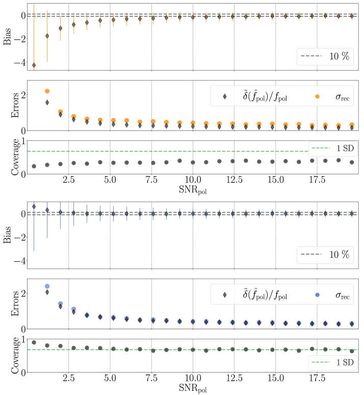
Figure 9: Results for the estimation of $f_{\mathrm{pol}}$ for the noise subtraction method (upper figure) and the Rice-distribution method (lower figure) up to SNR_pol=20. In the upper plots of the figures, we show the bias together with the error bar given by $\sigma_{\mathrm{rec}}$, as described in the text. In the middle plots, the resolution of each bin is compared with $\tilde{\delta}(\hat{f})/f$ of the same bin. The coverage of the uncertainties (eqn. 23), together with its error normalized to the number of entries of the bins, are shown in the lower plots and should ideally amount to 68%.

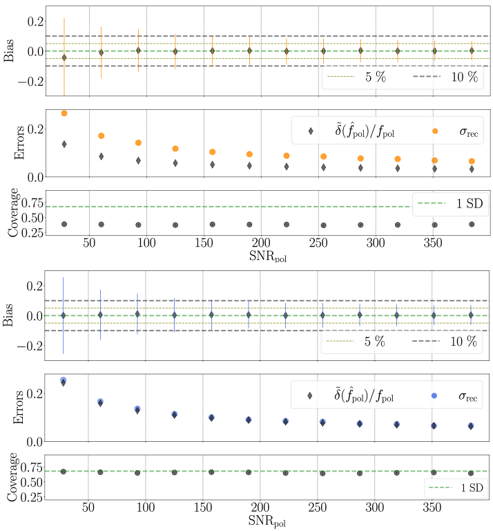
Figure 10: Results for the estimation of $f_{\mathrm{pol}}$ for the noise subtraction method (upper figure) and the Rice-distribution method (lower figure) up to SNR=400.

5.2 Polarisation Fluence $f_{\mathrm{pol}}$

For each electric field component of the data set, we evaluate the fluence estimators $\hat{f}_{\mathrm{pol}}$ and their uncertainties $\delta(\hat{f}_{\mathrm{pol}})$, together with the corresponding reference values $f_{\mathrm{pol}}$, and the associated signal-to-noise ratios $\mathrm{SNR}_{\mathrm{pol}}$. Once we have calculated the ratios $\psi=\frac{\hat{f}_{\mathrm{pol}}}{f_{\mathrm{pol}}}$, we look at different intervals of signal-to-noise ratio. We combine the data irrespective of the polarisation, meaning that we do not distinguish between EW, NS, and V components separately, but we collect all the ratios $\psi$ belonging to a certain SNR range. To reduce the impact of outliers, in each SNR interval, we calculate $\widetilde{\psi}$, the median value of $\psi$. Finally, we define the average reconstruction bias in the bin as $\mathrm{Bias}=\widetilde{\psi}-1$. To describe the dispersion of each bin, we use the interquartile range (i.q.r.) of the bin distribution. We calculate the equivalent standard deviation as $\sigma_{\mathrm{rec}}\approx\frac{\mathrm{i.q.r.}}{1.35}$. As shown in figure 9, where SNR values up to 20 are investigated, we found that the noise subtraction method is characterized by a negative bias up to about SNR=12. In many works, SNR values of at least 10 are required for higher-level analyses [1]. Note that the bias rapidly increases with decreasing SNR. For values above SNR=12, the bias remains below 10%, and is therefore acceptable. In comparison, the absolute value of the bias of the Rice-distribution method is contained within $10\%$ for SNR values approximately above 1.6, as shown in figure 9. The bias below this value is probably due to a combination of the estimator intrinsic bias discussed in sec. 4.4, and the lack of RFI suppression. Note that the Rice-distribution method allows for the estimation of null fluences (see eqn.14), whereas the estimation of the noise subtraction will result in negative and unphysical values. This is also why our method shows an impressive improvement at the lowest SNR values of the figure, even though the standard deviations of the two methods are comparable there.

We now focus on the uncertainty estimation of the two methods. We compare $\tilde{\delta}(\hat{f}_{\mathrm{pol}})/f_{\mathrm{pol}}$, the median value of the relative uncertainties of each bin, with $\sigma_{\mathrm{rec}}$. For unbiased estimators, we would expect the uncertainties to reflect the reconstruction resolution. As shown in figure 9, this is not the case for the noise subtraction method. In the region where the fluence estimation is on average unbiased, the uncertainties result to be systematically underestimated. To further corroborate this conclusion, we investigate the uncertainty coverage of the method. We define the coverage as the percentage of data points satisfying the condition:

$$f_{\mathrm{pol}}\in[\hat{f}_{\mathrm{pol}}-\delta(\hat{f}_{\mathrm{pol}}),\hat{f}_{\mathrm{pol}}+\delta(\hat{f}_{\mathrm{pol}})].$$ (23)

We notice that the error coverage of the noise subtraction method oscillates between 25% and 45%. On the contrary, the uncertainties of the Rice-distribution method reflect an average coverage of about 70%, which is close to the classical definition of one standard deviation (SD) coverage. We found that for higher values of SNR, both methods converge to a reconstruction bias below 5%, as shown in figure 10, where the region up to SNR=400 is studied. For a fair comparison, in all of the plots of the figure, we exclude the data points corresponding to SNR${}_{\mathrm{pol}}<$12. It is interesting to notice that, once more, the noise subtraction method exhibits a systematic underestimation of the uncertainties. The average coverage is about 40%, while our method provides a more consistent way of uncertainty estimation, with a coverage approaching the desired 68%.

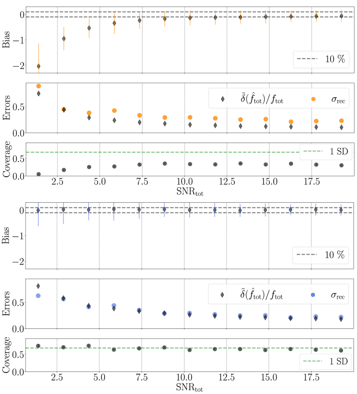
Figure 11: Results for the estimation of $f_{\mathrm{tot}}$ for the noise subtraction method (upper figure) and the Rice-distribution method (lower figure) up to SNR=20.

5.3 Total Fluence $f_{\mathrm{tot}}$

In this section, we repeat the analysis presented in the previous section, adapting it to the estimation of the total fluence evaluated at the antenna position. Since the estimator of $f_{\mathrm{tot}}$ is a linear combination of the fluence estimators obtained individually from each electric field component, we expect the noise subtraction method to still show a strong bias at low SNR values. Indeed, as shown in figure 11, the method can be considered on average unbiased starting only from about SNR=12.5. As already mentioned, typically an SNR threshold cut around this value is introduced to exclude the data from further analyses. The uncertainties derived from the method are underestimated, with an average coverage of about 40%.

We can draw the same conclusion for higher values of SNR, despite the bias and the resolution becoming smaller (see figure 12, where we show the SNR_tot range from 12.5 up to 400). In contrast, the method we implemented can be considered on average unbiased and the error coverage fluctuates around 68% (see figures 11 and 12).

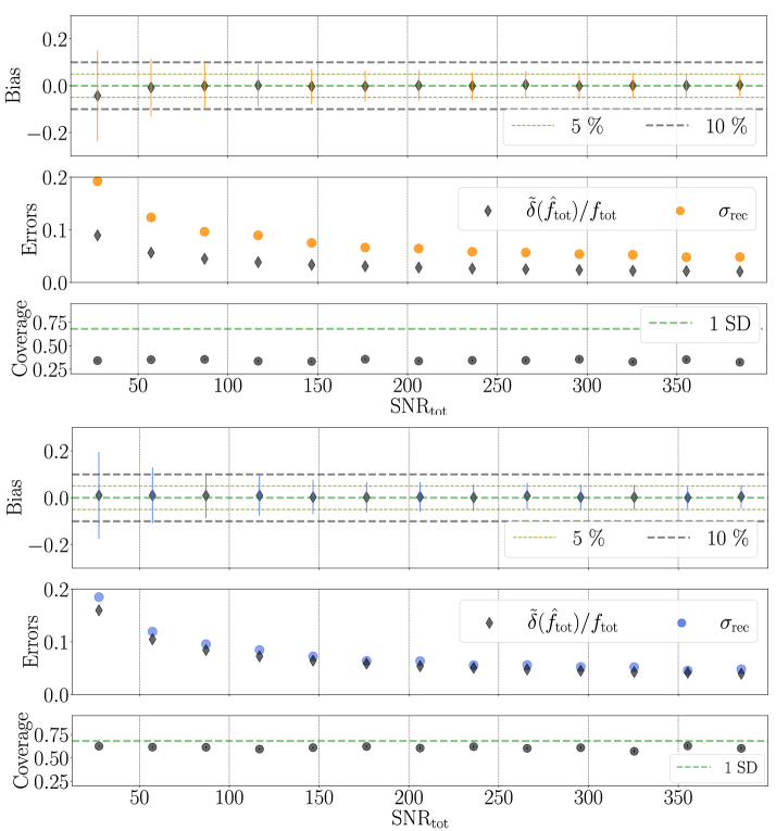
Figure 12: Results for the estimation of $f_{\mathrm{tot}}$ for the noise subtraction method (upper figure) and the Rice-distribution method (lower figure) up to SNR=400.

6 Conclusions

In this work, we showed that the noise-subtraction method conventionally used to reconstruct the energy fluence is strongly biased at the low SNR values and that the derived uncertainties are underestimated. We developed a method based on Rice distributions for a better estimation of the fluence and its uncertainty. With the Rice-distribution method, we achieve an average bias below 10% down to signal-to-noise ratios of about 1.6 at polarisation level, while the estimation of the fluence at the antenna level remains on average within 10% even at the lowest values investigated. We also significantly improve the estimation of the uncertainties, reaching a reliable coverage of about 68%. With the Rice-distribution method, the estimation of energy fluence and its uncertainty can thus be significantly improved, and signal-to-noise cuts can be lowered or possibly completely avoided in higher-level analyses.

The Rice-distribution method is generic and can be applied to any kind of radio observations of air showers and in-ice cascades. Since the method is not constrained by the frequency bandwidth of sensitivity, radio experiments in the field of astroparticle physics can make use of it. Among others, the Pierre Auger Observatory, RNO-G [4], LOFAR, ANITA, GRAND[16], SKA[15], and the IceCube Neutrino Observatory[17] could benefit from adopting this approach. The statistical background employed to develop the fluence estimation method can be further exploited, as we show in the Appendix B. There, we describe how to estimate the signal amplitude employing the Rice likelihood function. Further improvements and applications are still feasible by combining this statistical approach and the signal modeling in the frequency domain. Additional developments are possible in the time domain, too.

Appendix A Derivation of the Fluence Estimator and its Uncertainty

In the following, we derive the energy fluence estimator and its uncertainty presented in sec. 4.3. Let us consider the case of a monochromatic signal. Setting K=1 for simplicity, equations 10, 12 can be written as:

$$f_{s}=s^{2}(\nu_{0})\equiv s^{2},\quad\hat{f}_{\mathrm{a}}=a^{2}(\nu_{0})\equiv a^{2},$$ (24)

where $s$ denotes the monochromatic signal, and $a$ is the measured amplitude in the presence of random noise. We look for an estimator of the parameter $f_{s}$ of the form $\hat{f}_{s}\propto a^{2}$.

As described in sec. 4.2, the random variable $a$ follows the Rice distribution, i.e. $a\sim\mathcal{R}ice(s,\sigma)$, with $\sigma$ being the standard deviation of the noise. To obtain an estimator in terms of the squared amplitude, we derive the PDF of the random variable $a^{2}$ starting from the PDF of $a$. To do so, first, we standardize the variable $a$ introducing the change of variable $b=a/\sigma$. The variable $b$ also follows a Rice distribution, i.e. $b\sim\mathcal{R}ice(s/\sigma,1)$, that is equivalent to a non-central $\chi$ distribution with two degrees of freedom (DF) and non-centrality parameter $\lambda=s/\sigma$:

$$b\sim\mathcal{R}ice(s/\sigma,1)=\chi_{\mathrm{nc}}(DF=2,\lambda=s/\sigma).$$ (25)

Thus, the variable $b^{2}$ follows a non-central $\chi^{2}$ distribution of the form:

$$b^{2}\sim\chi^{2}_{\mathrm{nc}}(DF=2,\lambda=(s/\sigma)^{2}).$$ (26)

Note that for $s^{2}\gg\sigma^{2}$ we can approximate the distribution with a normal distribution.

Noise Fluence Estimator

The evaluation of the signal estimator requires the knowledge of the estimator of the noise fluence. We estimate the noise by sampling the trace in $N\approx 60$ noise windows. Each i-th window provides a measured noise amplitude $n_{i}$, that, as described in sec. 4.2, we assume to be Rayleigh-distributed. The variable $(n_{i}/\sigma)^{2}$ follows a chi-square distribution having two degrees of freedom. Thus, the random variable $T=\sum_{i=0}^{N-1}(n_{i}/\sigma)^{2}$ follows a chi-square distribution having $DF=2\,N$, that for large $N$ can be approximated by a normal distribution having mean value $\mu=2\,N$ and variance Var=4 N. We define the estimator of the noise fluence as the sample mean of the squared noise amplitudes:

$$\hat{f}_{\mathrm{n}}=\frac{1}{N}\sum_{i=0}^{N-1}n_{i}^{2}=\frac{\sigma^{2}}{N}T,$$ (27)

which follows a normal distribution with mean value $\mu=2\,\sigma^{2}$ and variance Var=4 $\sigma^{4}/N$. By defining $f_{\mathrm{n}}:=2\,\sigma^{2}$, it follows that $\hat{f}_{\mathrm{n}}$ is an unbiased estimator of $f_{\mathrm{n}}$. For $N\approx 60$, its relative uncertainty will fluctuate around 13%.

Signal Fluence Estimator

Knowing the expected value of $b^{2}$, we can derive the expected value of $\hat{f}_{\mathrm{a}}$:

$$\begin{split}E(b^{2})=2+(s/\sigma)^{2}\\ \rightarrow\,E(\hat{f}_{\mathrm{a}})=E(a^{2})=\sigma^{2}\,E(b^{2})=2\,\sigma^{2}+s^{2}.\end{split}$$ (28)

Following the same reasoning, for the noise estimator we obtain by setting $s=0$:

$$E(\hat{f}_{\mathrm{n}})=2\,\sigma^{2}:=f_{\mathrm{n}}.$$ (29)

Estimating the signal fluence as $\hat{f}_{\mathrm{s}}=\hat{f}_{\mathrm{a}}-\hat{f}_{\mathrm{n}}$, its mean value will be:

$$E(\hat{f}_{\mathrm{s}})=E(\hat{f}_{\mathrm{a}})-E(\hat{f}_{\mathrm{n}})=s^{2}=f_{\mathrm{s}},$$ (30)

meaning that such an estimator would be unbiased. Since the energy fluence has to be positively defined, we have to introduce the condition:

$$\hat{f}_{\mathrm{s}}=0\quad\hat{f}_{\mathrm{a}}<\hat{f}_{\mathrm{n}}.$$ (31)

As discussed in sec. 4.4, the above condition introduces a positive bias that can be neglected for $R=f_{\mathrm{s}}/f_{\mathrm{n}}>2$.

Signal Fluence Uncertainty

Starting from the variance of $b^{2}$, we derive the variance of $a^{2}$:

$$\begin{split}\mathrm{Var}(b^{2})=2\,\big{(}2+2\,(s/\sigma)^{2}\big{)}\\ \rightarrow\quad\mathrm{Var}(a^{2})=\sigma^{4}\,\mathrm{Var}(b^{2})=2\,\sigma^{2}(2\,\sigma^{2}+2\,s^{2}).\end{split}$$ (32)

To calculate the variance of $\hat{f}_{\mathrm{s}}$ from the variance of $a^{2}$, we have to make the following assumptions:

• The noise fluence is measured with much better precision than $a^{2}$. This can be considered a valid assumption since the variable $a$ is a single measurement (from the signal window), while the noise fluence is estimated through $N\approx 60$ noise windows;

• The probability of hitting the physical limit of eqn.31 is negligible, i.e. we are assuming $R>2$;

• The non-centrality parameter $(s/\sigma^{2})$ is large, meaning that $a^{2}$ and $b^{2}$ are normal in a good approximation. In other words, we are again assuming $R$ to be large.

Under these assumptions, the variance of $\hat{f}_{\mathrm{s}}$ is:

$$\mathrm{Var}(\hat{f}_{\mathrm{s}})=\mathrm{Var}(a^{2})\approx\hat{f}_{\mathrm{n}}\big{(}\hat{f}_{\mathrm{n}}+2\,\hat{f}_{\mathrm{s}}\big{)},$$ (33)

where we approximate the unknown parameters as $s^{2}$$\approx$$\hat{f}_{\mathrm{s}}$ and $2\,\sigma^{2}$$\approx\hat{f}$_n. We define the confidence interval as $\hat{f}_{\mathrm{s}}\pm\delta(\hat{f}_{\mathrm{s}})$, with:

$$\delta(\hat{f}_{\mathrm{s}})=\sqrt{\mathrm{Var}(\hat{f}_{\mathrm{s}})}=\sqrt{\hat{f}_{\mathrm{n}}\big{(}\hat{f}_{\mathrm{n}}+2\,\hat{f}_{\mathrm{s}}\big{)}}.$$ (34)

Appendix B Spectral Amplitude Estimator and its Uncertainty

In this work, we showed how to apply the theoretical background described in sec. 4.2 to recover the signal fluence and estimate its uncertainty. However, the formalism has much more potential to exploit. Here we introduce the Rice likelihood function and provide an application example. In particular, we present a method to estimate the signal spectral amplitude and its uncertainty, but, as already mentioned, the formalism can be adopted both in time and frequency domains.

Let us consider the case of a single-frequency signal $s_{0}\equiv\,s(\nu_{0})$, with $a_{0}\equiv\,a(\nu_{0})$ being the spectral amplitude measured in the signal window defined in sec. 4.1, and $\hat{\sigma}_{0}$ the estimator of the noise level of the same frequency. The Rice likelihood function will be:

$$L(s\mid a=a_{0},\sigma=\hat{\sigma}_{0})=\frac{a}{\sigma^{2}}\,\mathrm{exp}\left(-\frac{a^{2}+s^{2}}{2\sigma^{2}}\right)\,I_{0}\left(\frac{as}{\sigma^{2}}\right),$$ (35)

where $s\geq 0$. We evaluate $\hat{\sigma}_{0}$ making use of the $N$ noise windows, as defined in sec. 4.1:

$$\hat{\mu}_{0}=\frac{1}{N}\sum_{i=0}^{N-1}a_{i}(v_{0})\,\,\rightarrow\,\,\hat{\sigma}_{0}\equiv\mu_{0}\sqrt{2/\pi},$$ (36)

where in the last equivalence we assumed the noise to be Rayleigh-distributed with scale parameter $\sigma_{0}$ and mean value $\mu_{0}$. We define the estimator of the parameter $s_{0}$ as the amplitude $\hat{s}_{\mathrm{ML}}$ that maximizes $L(s)$. Since it is not possible to solve analytically $\frac{dL(s)}{ds}\Bigr{|}_{\begin{subarray}{c}s=\hat{s}_{\mathrm{ML}}\end{subarray}}$=0, we recommend the reader to run a scalar minimization algorithm to find the minimum of the cost function $J(s)=-\mathrm{ln\big{(}}L(s)\mathrm{\big{)}}$. To avoid unphysical solutions, such as negative results, and to make the minimization process reliable, we exploit a bounded solver. We set as bounds $[a_{0}-1.5\cdot\hat{\sigma}_{0},a_{0}+1.5\cdot\hat{\sigma}_{0}]$. There are some intervals where it is not strictly necessary to run the minimizer solver. In particular, for $a_{0}/\hat{\sigma}_{0}\leq\sqrt{2}$, the likelihood function has its maximum at zero, i.e. $\hat{s}_{\mathrm{ML}}=0$. For larger ratios, as $a_{0}/\hat{\sigma}_{0}\geq$4, we can approximate $L(s)$ by a normal distribution having SD=$\hat{\sigma}_{0}$ and centered in $\sqrt{a_{0}^{2}-\hat{\sigma}_{0}^{2}}$. In this case, one can evaluate the maximum likelihood solution as $\hat{s}_{\mathrm{ML}}\approx\sqrt{a_{0}^{2}-\hat{\sigma}_{0}^{2}}$.

To evaluate the estimator uncertainty $\delta$, we work in Gaussian approximation. First, we approximate the likelihood $cost$ function as:

$$\begin{split}J(s)\approx J(\hat{s}_{\mathrm{ML}})+(s-\hat{s}_{\mathrm{ML}})\cdot\frac{\partial J(s)}{\partial s}\Bigr{|}_{\begin{subarray}{c}s=\hat{s}_{\mathrm{ML}}\end{subarray}}+\\ +(s-\hat{s}_{\mathrm{ML}})^{2}\cdot\frac{1}{2}\frac{\partial^{2}J(s)}{\partial s^{2}}\Bigr{|}_{\begin{subarray}{c}s=\hat{s}_{\mathrm{ML}}\end{subarray}},\end{split}$$ (37)

where the first two terms are null by definition. Since the $cost$ function of a Gaussian distribution is a parabolic function, we can approximate $J(s)$ to a parabola as well. This would lead to the following system of equations:

$$\begin{cases}\begin{split}J(s)=(s-\hat{s}_{\mathrm{ML}})^{2}\cdot\frac{1}{2}\frac{\partial^{2}J(s)}{\partial s^{2}}\Bigr{|}_{\begin{subarray}{c}s=\hat{s}_{\mathrm{ML}}\end{subarray}}\\ =\delta^{2}\cdot\frac{1}{2}\frac{\partial^{2}J(s)}{\partial s^{2}}\Bigr{|}_{\begin{subarray}{c}s=\hat{s}_{\mathrm{ML}}\end{subarray}}\end{split}\\ J(s)\approx\,k^{2}\quad\rightarrow\quad\delta=k\cdot SD\\ \end{cases}$$ (38)

Finally, by requiring a one-sigma interval, i.e. $\delta$=1 SD, the solution of eqn. 38 is given by:

$$\delta=1\Bigg{/}\sqrt{\frac{1}{2}\frac{\partial^{2}J(s)}{\partial s^{2}}\Bigr{|}_{\begin{subarray}{c}s=\hat{s}_{\mathrm{ML}}\end{subarray}}}.$$ (39)

Appendix C Table of Variables and Notation

Generic Variables
$E_{\mathrm{pol}}$	Electric field component in the chosen coordinates system
$f_{\mathrm{pol}}$	Energy fluence relative to the considered electric field component
$f_{\mathrm{tot}}$	Total energy fluence at the antenna position
SNRpol	Signal-to-noise ratio relative to the considered electric field component
SNRtot	Signal-to-noise ratio calculated over all the electric field components
Notation
$y$	Unknown parameter (true value)
$\hat{y}$	Estimator of the parameter (or measurement)
$\delta\big{(}\hat{y}\big{)}$	Uncertainty on the estimator (or measurement)
$\overline{h}$	Mean value of the variable
$\tilde{h}$	Median value of the variable
Rice-distribution Variables (fixed frequency or time)
$s$	Signal amplitude in the absence of noise
$a$	Measured amplitude of the signal in the presence of noise
$f_{\mathrm{s}},\hat{f}_{\mathrm{s}}$	Signal energy fluence, its estimator
$f_{\mathrm{n}},\hat{f}_{\mathrm{n}}$	Noise energy fluence, its estimator
$\hat{f}_{\mathrm{a}}$	Signal energy fluence measured in the presence of noise

References

- Aab et al. [2016a] Aab, A., et al. (Pierre Auger Collaboration), 2016a. Energy estimation of cosmic rays with the engineering radio array of the pierre auger observatory. Phys. Rev. D 93, 122005. URL: https://link.aps.org/doi/10.1103/PhysRevD.93.122005, doi:10.1103/PhysRevD.93.122005.
- Aab et al. [2016b] Aab, A., et al. (Pierre Auger Collaboration), 2016b. Measurement of the radiation energy in the radio signal of extensive air showers as a universal estimator of cosmic-ray energy. Phys. Rev. Lett. 116, 241101. URL: https://link.aps.org/doi/10.1103/PhysRevLett.116.241101, doi:10.1103/PhysRevLett.116.241101.
- Abreu et al. [2011] Abreu, P., et al., 2011. Advanced functionality for radio analysis in the offline software framework of the pierre auger observatory. Nuclear Instruments and Methods in Physics Research Section A: Accelerators, Spectrometers, Detectors and Associated Equipment 635, 92–102. URL: http://dx.doi.org/10.1016/j.nima.2011.01.049, doi:10.1016/j.nima.2011.01.049.
- Aguilar et al. [2021] Aguilar, J., et al., 2021. Design and sensitivity of the radio neutrino observatory in greenland (rno-g). Journal of Instrumentation 16, P03025. URL: http://dx.doi.org/10.1088/1748-0221/16/03/P03025, doi:10.1088/1748-0221/16/03/p03025.
- Corstanje et al. [2021] Corstanje, A., et al., 2021. Depth of shower maximum and mass composition of cosmic rays from 50 pev to 2 eev measured with the lofar radio telescope. Phys. Rev. D 103, 102006. URL: https://link.aps.org/doi/10.1103/PhysRevD.103.102006, doi:10.1103/PhysRevD.103.102006.
- Glaser [2017] Glaser, J., 2017. Absolute Energy Calibration of the Pierre Auger Observatory using Radio Emission of Extensive Air Showers. Ph.D. thesis. RWTH Aachen University.
- Goodman [2000] Goodman, J.W., 2000. Statistical Optics. Wiley Classics Library.
- Harris [1978] Harris, F., 1978. On the use of windows for harmonic analysis with the discrete fourier transform. Proceedings of the IEEE 66, 51–83. doi:10.1109/PROC.1978.10837.
- Heck et al. [1998] Heck, D., Knapp, J., Capdevielle, J.N., Schatz, G., Thouw, T., 1998. CORSIKA: a Monte Carlo code to simulate extensive air showers. FZKA Report 6019, Forschungszentrum Karlsruhe .
- Huege [2016] Huege, T., 2016. Radio detection of cosmic ray air showers in the digital era. Physics Reports 620, 1–52.
- Huege [2023] Huege, T. (Pierre Auger), 2023. The Radio Detector of the Pierre Auger Observatory – status and expected performance, in: EPJ Web Conf., Ultra High Energy Cosmic Rays (UHECR 2022). doi:https://doi.org/10.1051/epjconf/202328306002.
- Huege et al. [2013] Huege, T., Ludwig, M., James, C.W., 2013. Simulating radio emission from air showers with CoREAS. AIP Conf. Proc. 1535, 128.
- Karastathis et al. [2023] Karastathis, N., et al., 2023. Using pulse-shape information for reconstructing cosmic-ray air showers and validating antenna responses with lofar and ska, in: 38th International Cosmic Ray Conference (ICRC2023) - Cosmic-Ray Physics (Indirect, CRI), Scuola Internazionale Superiore di Studi Avanzati (SISSA). pp. Art.–Nr.: 487. doi:10.22323/1.444.0487. 51.13.04; LK 01.
- Kobal [2001] Kobal, M., 2001. A thinning method using weight limitation for air-shower simulations. Astropart. Phys. 15, 259–273.
- de Lera Acedo et al. [2016] de Lera Acedo, E., Faulkner, A., Bij de Vaate, J., 2016. Ska low frequency aperture array, in: 2016 United States National Committee of URSI National Radio Science Meeting (USNC-URSI NRSM), pp. 1–2. doi:10.1109/USNC-URSI-NRSM.2016.7436228.
- Álvarez Muñiz et al. [2019] Álvarez Muñiz, J., et al., 2019. The giant radio array for neutrino detection (grand): Science and design. Science China Physics, Mechanics & Astronomy 63. URL: http://dx.doi.org/10.1007/s11433-018-9385-7, doi:10.1007/s11433-018-9385-7.
- Oehler and Turcotte-Tardif [2021] Oehler, M., Turcotte-Tardif, R., 2021. Development of a scintillation and radio hybrid detector array at the south pole. URL: https://arxiv.org/abs/2107.09983, arXiv:2107.09983.
- Ostapchenko [2011] Ostapchenko, S., 2011. Monte Carlo treatment of hadronic interactions in enhanced Pomeron scheme: QGSJET-II model. Phys. Rev. D 83, 128.
- Schlüter and Huege [2023] Schlüter, F., Huege, T., 2023. Signal model and event reconstruction for the radio detection of inclined air showers. JCAP 01, 008. doi:10.1088/1475-7516/2023/01/008, arXiv:2203.04364.
- Schlüter [2023] Schlüter, F. (Pierre Auger), 2023. Expected performance of the AugerPrime Radio Detector, in: Proceedings of 9th International Workshop on Acoustic and Radio EeV Neutrino Detection Activities — PoS(ARENA2022), p. 028. doi:10.22323/1.424.0028.
- Schoorlemmer et al. [2016] Schoorlemmer, H., et al., 2016. Energy and flux measurements of ultra-high energy cosmic rays observed during the first anita flight. Astroparticle Physics 77, 32–43. URL: http://dx.doi.org/10.1016/j.astropartphys.2016.01.001, doi:10.1016/j.astropartphys.2016.01.001.
- Schröder [2012] Schröder, F., 2012. On noise treatment in radio measurements of cosmic ray air showers. Nucl. Instr. and Meth. A 662, S238--S241. doi:https://doi.org/10.1016/j.nima.2010.11.009.
- Schröder [2017] Schröder, F.G., 2017. Radio detection of cosmic-ray air showers and high-energy neutrinos. Progress in Particle and Nuclear Physics 93, 1–68. URL: http://dx.doi.org/10.1016/j.ppnp.2016.12.002, doi:10.1016/j.ppnp.2016.12.002.
- Tukey [1967] Tukey, J.W., 1967. An introduction to the calculations of numerical spectrum analysis, in: Harris, B. (Ed.), Spectral Analysis of Time Series. New York: Wiley, pp. 25--46.