Managing CO₂ under global and country-specific net-zero emissions targets in Europe

Abstract

The European Union (EU) is committed to achieving carbon neutrality by 2050. This requires capturing CO₂, eventually transporting it to different regions, to then either convert it into valuable products or sequester it underground. While the target is set for the EU as a whole, a significant part of the governance and strategy remains in the individual member states. Using the networked sector-coupled model PyPSA-Eur, we explored the impacts of imposing net-zero emissions globally for the entire EU versus imposing carbon neutrality for each country. Under a global CO₂ target, some countries remain net CO₂ emitters, while others become net CO₂ absorbers. Forcing net-zero emissions in every country increases system cost by 1.4%, demands varied CO₂ prices, and triggers higher investment in direct air capture and renewable capacities. In both scenarios, a significant portion of the captured CO₂ is transported across Europe either directly in CO₂ pipelines or indirectly via solid biomass or synthetic methane gas, methanol, and oil.

[mpe] organization = Department of Mechanical and Production Engineering, Aarhus University, addressline = Katrinebjergvej 89, city = Aarhus, postcode = 8200, country = Denmark

[novo] organization = Novo Nordisk Foundation CO₂ Research Center, addressline = Gustav Wieds Vej 10, city = Aarhus, postcode = 8000, country = Denmark

1 Introduction

The European Union (EU) has committed to achieving climate neutrality by 2050 [1], aiming for an economy with net-zero greenhouse gas (GHG) emissions. Given that carbon dioxide (CO₂) constitutes about 75% of the total GHG emissions globally [2], understanding how this chemical compound could be managed across Europe in a future climate-neutral system is crucial. The EU is implementing a comprehensive policy framework with intermediate steps to reduce CO₂ emissions by at least 55% by 2030 and 90% by 2040 relative to 1990 levels, as key milestones towards the 2050 goal [3]. This has led the EU Commission to propose, amongst other measures, that at least 50 MtCO₂ per year can be sequestered geologically by 2030 [4].

Although the Paris Agreement has been signed at the EU level, a significant part of the governance remains at a national level, with each country deciding its own strategy and setting its decarbonisation goals for 2050 and intermediate steps. This distributed decision process is typically absent when modelling future scenarios. Both Energy System Models (ESMs) and Integrated Assessment Models (IAMs) commonly calculate optimal decarbonisation scenarios in which carbon neutrality is imposed at a global level and all the modelled regions contribute to the global objective. This yields non-uniform contributions to GHG mitigation and carbon dioxide removal (CDR) from the different regions raising questions about the fairness of the attained solution.

For the European electricity sector, scenarios with country-level CO₂ emissions targets have been explored in Schwenk-Nebbe et al. [5] and Pedersen et al. [6]. In both works, a large variation is found in the CO₂ price required in each country for the same CO₂ target, highlighting that the mitigation potential, and consequently the need for CO₂ price or policy-driven transformations, is radically different amongst countries.

The problem is also seen at a global level. Strefler et al. [7] found that scenarios consistent with a 1.5 °C temperature increase involve a highly uneven distribution of CDR technologies across different continents. Furthermore, Bauer et al. [8] argues that uniform carbon pricing tend to impose high mitigation costs on developing and emerging economies. In their work, the authors discuss the trade-offs of a system with a uniform carbon pricing worldwide and financial transfers, a system with different carbon prices for each region without any financial transfer, and argue that a hybrid combination might be the best solution. The usage and uniformity of different CDR technologies in their model are also affected by the selected strategy.

Coming back to Europe, in Victoria et al. [9], the open sector-coupled model PyPSA-Eur is used to implement myopic transition paths with different carbon budgets, corresponding to temperature increments from 1.5 to 2 °C, and under a globally imposed limit on CO₂ emissions for the entire continent. They found that the technologies used to capture CO₂ are (in order of appearance): (i) point-source capture of industry process emissions, (ii) capture from biomass used for heating in the industry and combusted in combined heat and power (CHP) units, (iii) capture from methane gas used in the industry, and (iv) Direct Air Capture (DAC). Captured CO₂ is preferentially sequestered underground and used to produce synthetic oil using the Fischer-Tropsch process.

In Neumann et al. [10], PyPSA-Eur is extended to include an additional option to use CO₂ by converting it into synthetic methanol used by the shipping industry. In addition, the model is further extended in Hofmann et al. [11] to allow the endogenous built-in of a CO₂ network to transport CO₂ around the continent.

Acronym	Description
BECCS	Bioenergy with carbon capture and storage
CC	Carbon capture
CCUS	CO2 capture, usage, and storage
CDR	Carbon dioxide removal
CHP	Combined heat and power
CO2	Carbon dioxide
DAC	Direct air capture
DOC	Direct ocean capture
ENSPRESO	Energy system potentials for renewable energy sources
ENTSO-E	European network of transmission system operators for electricity
ESM	Energy system model
EU	European Union
GHG	Greenhouse gas
H2	Hydrogen
IAM	Integrated assessment model
JRC-EU-TIMES	Joint Research Centre European TIMES energy system model
LULUCF	Land use, land use change, and forestry
PHS	Pump hydro storage
PV	Photovoltaic
PyPSA	Python for power system analysis
PyPSA-Eur	Python for power system analysis for Europe
ROR	Run-of-river
SMR	Steam methane reforming

In this work, for the first time, we use a sector-coupled model of Europe including electricity, heating, land transport, aviation, shipping, industry, as well as industrial feedstock, and detailed carbon management to investigate country-wise CO₂ targets. We compare a climate-neutral European energy system with net-zero CO₂ emissions imposed globally for the whole of Europe versus locally for each country, and investigate the impact of these requirements on the technologies used to capture and convert CO₂, their optimal location and operation patterns, and on the underground sequestration of CO₂ in deep saline aquifers and depleted hydrocarbon reservoirs. Moreover, we evaluate the distribution of CO₂ emissions, the flows of energy and CO₂, and the required CO₂ prices to force more uniform scenarios.

2 Results and discussion

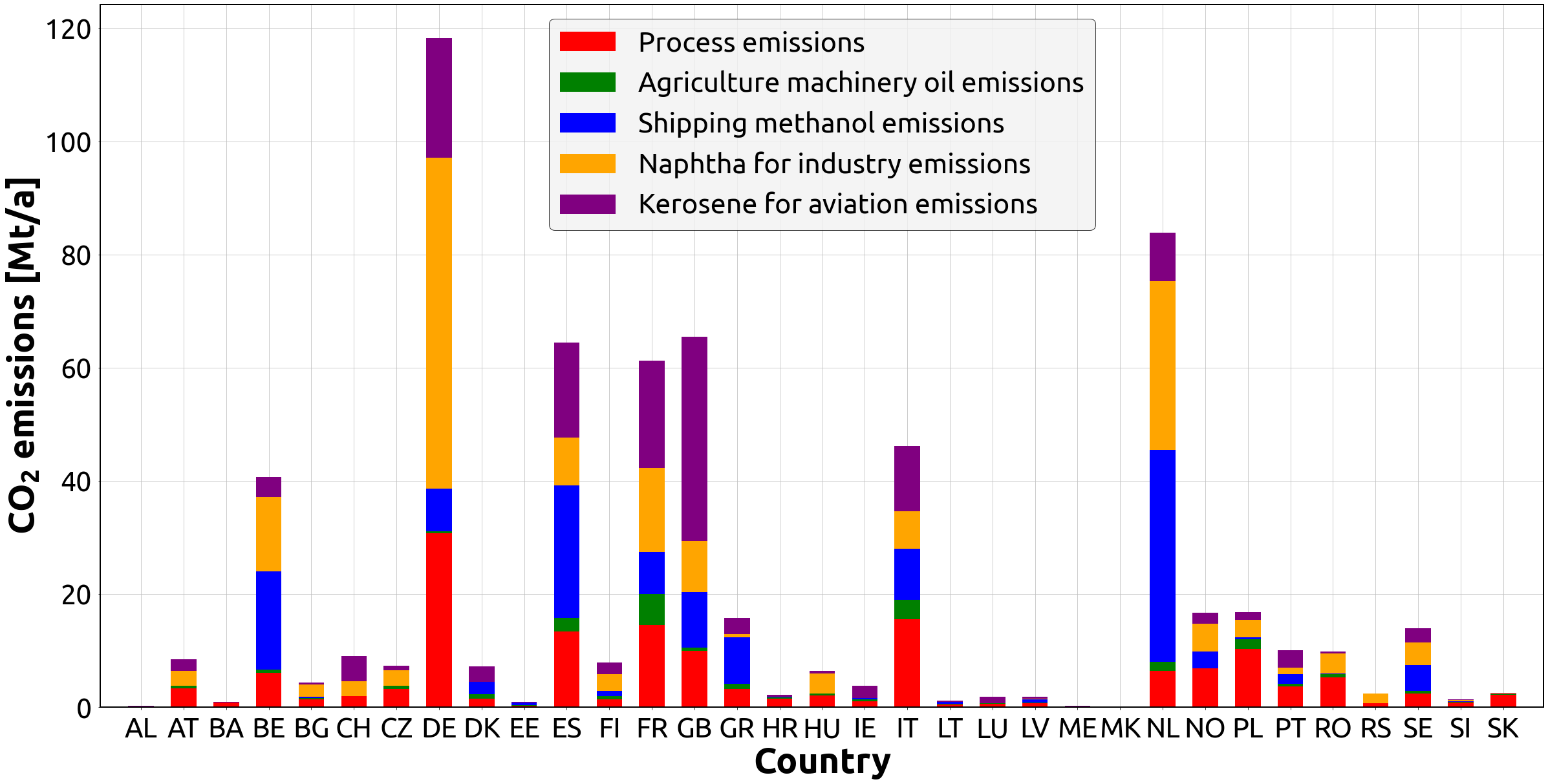
Figure S7: Exogenous CO₂ emissions per country and sector in both the global and local net-zero CO₂ emissions scenarios. CO₂ emissions total 634 Mt/a, with 153 Mt/a coming from process emissions, 23 Mt/a from oil for agriculture machinery, 135 Mt/a from methanol for shipping, 177 Mt/a from naphtha for industry, and 146 Mt/a from kerosene for aviation.

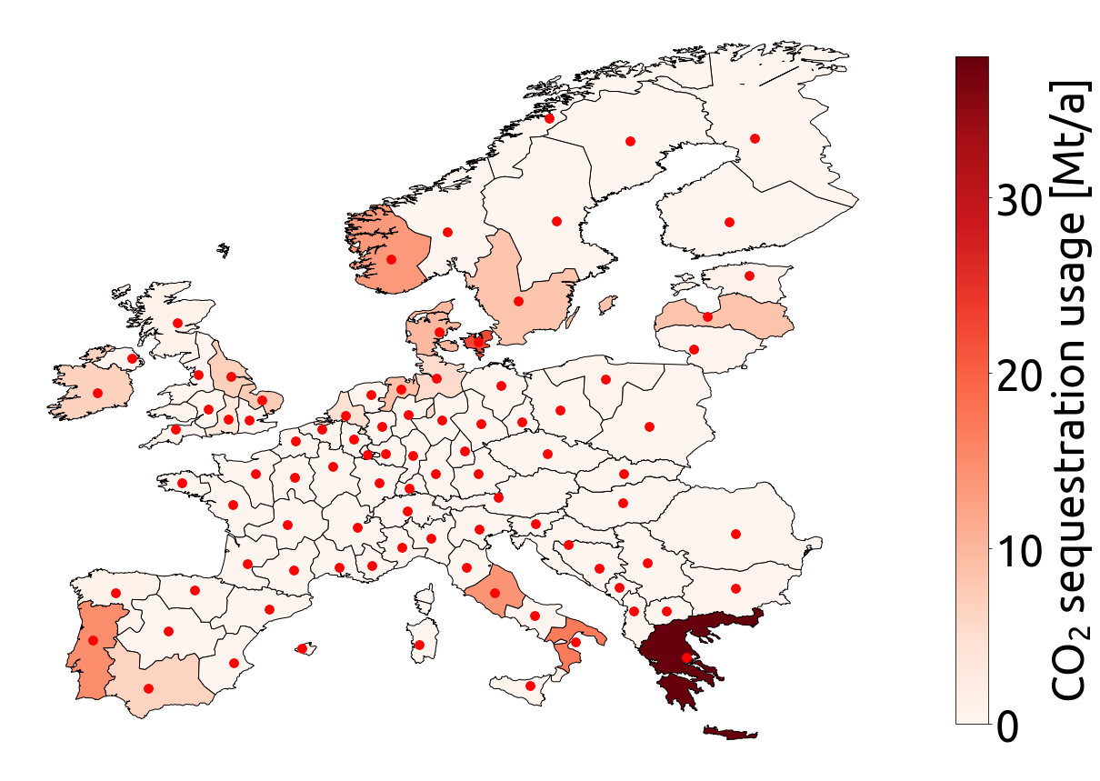
(a)

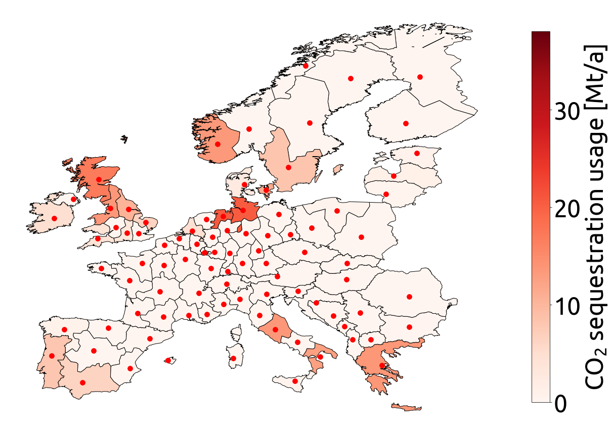
(b)

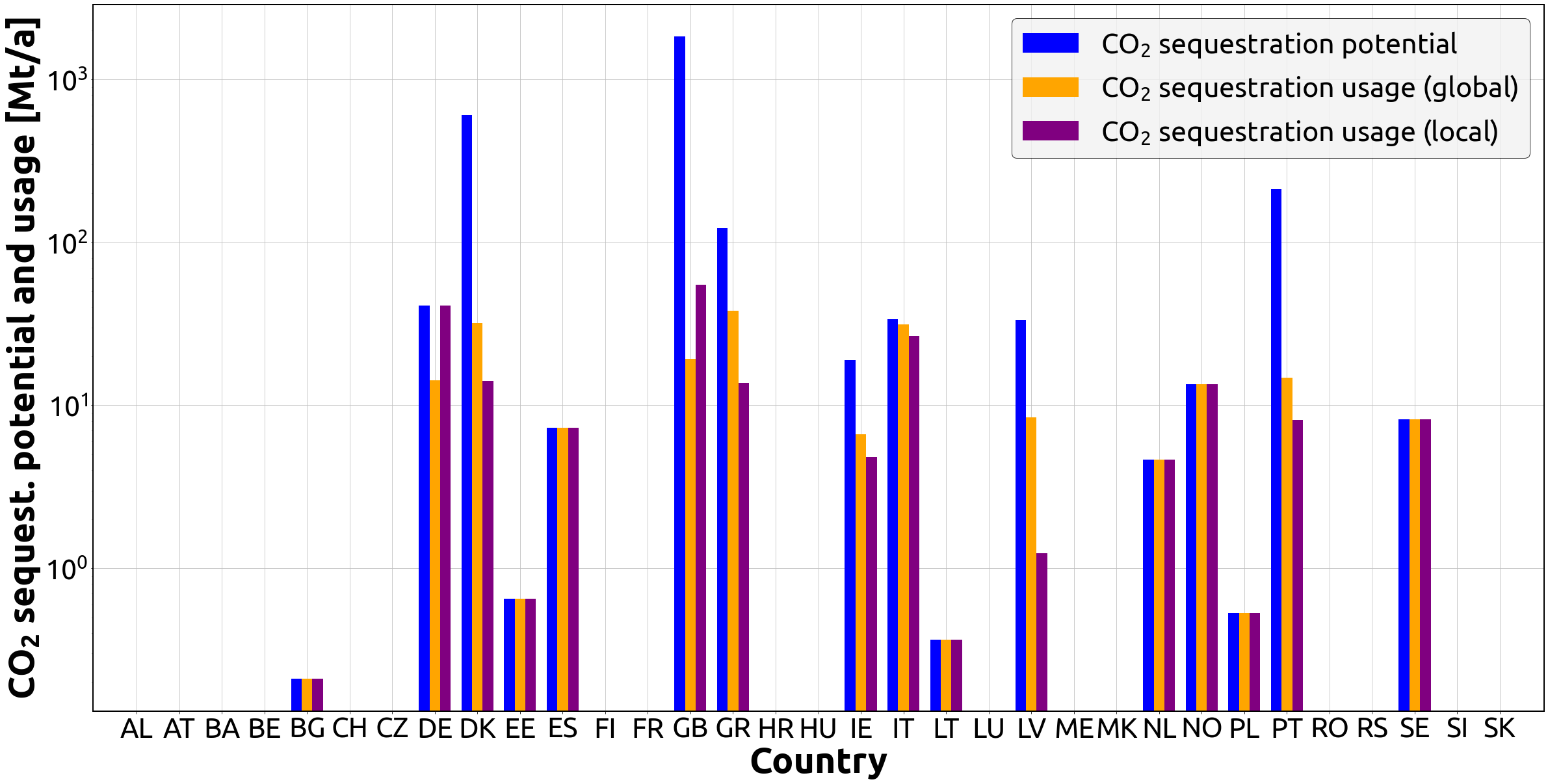
(c)

Figure S8: CO₂ underground sequestration usage across Europe in (a) the global net-zero CO₂ emissions scenario and (b) the local net-zero CO₂ emissions scenario, and (c) CO₂ underground sequestration potential per country and usage in the global and local net-zero CO₂ emissions scenarios. Despite the varying levels of sequestration usage amongst countries in the two scenarios, the conservative sequestration potential limit of 200 MtCO₂/a is fully exhausted in both scenarios.

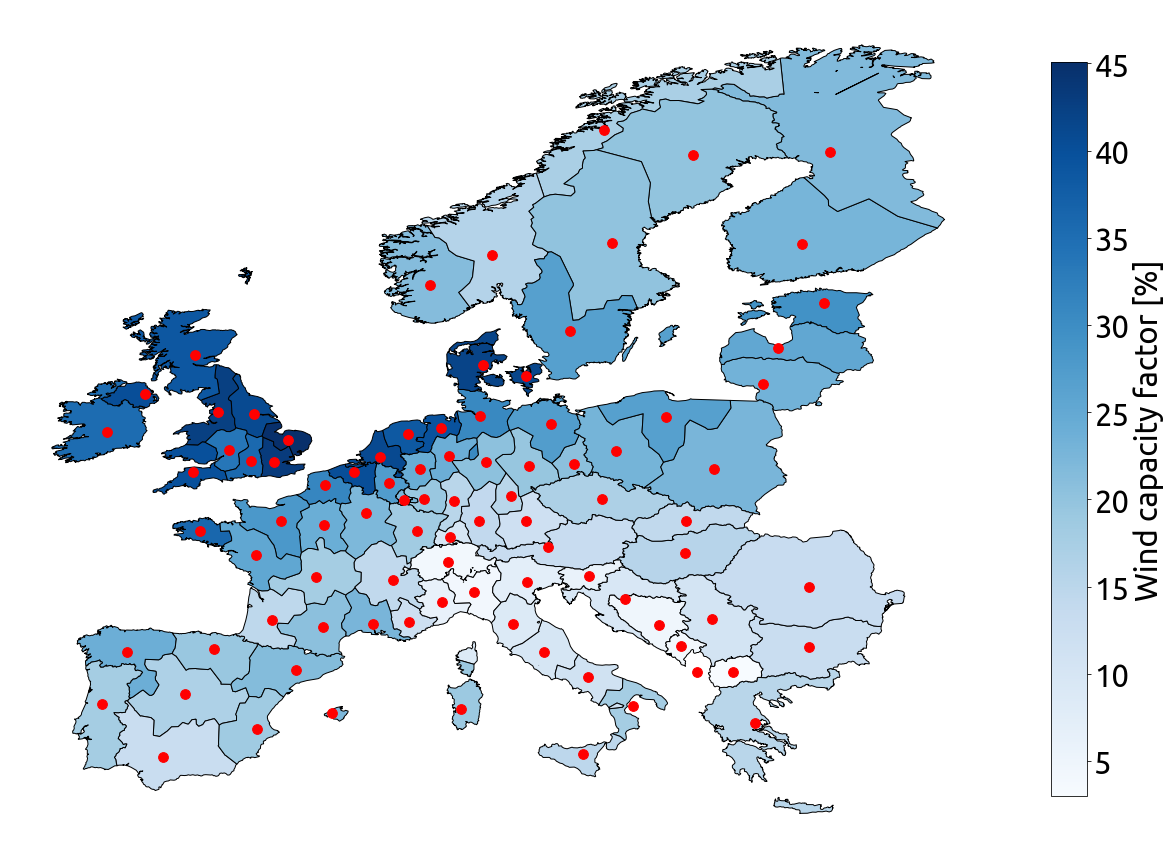
(a)

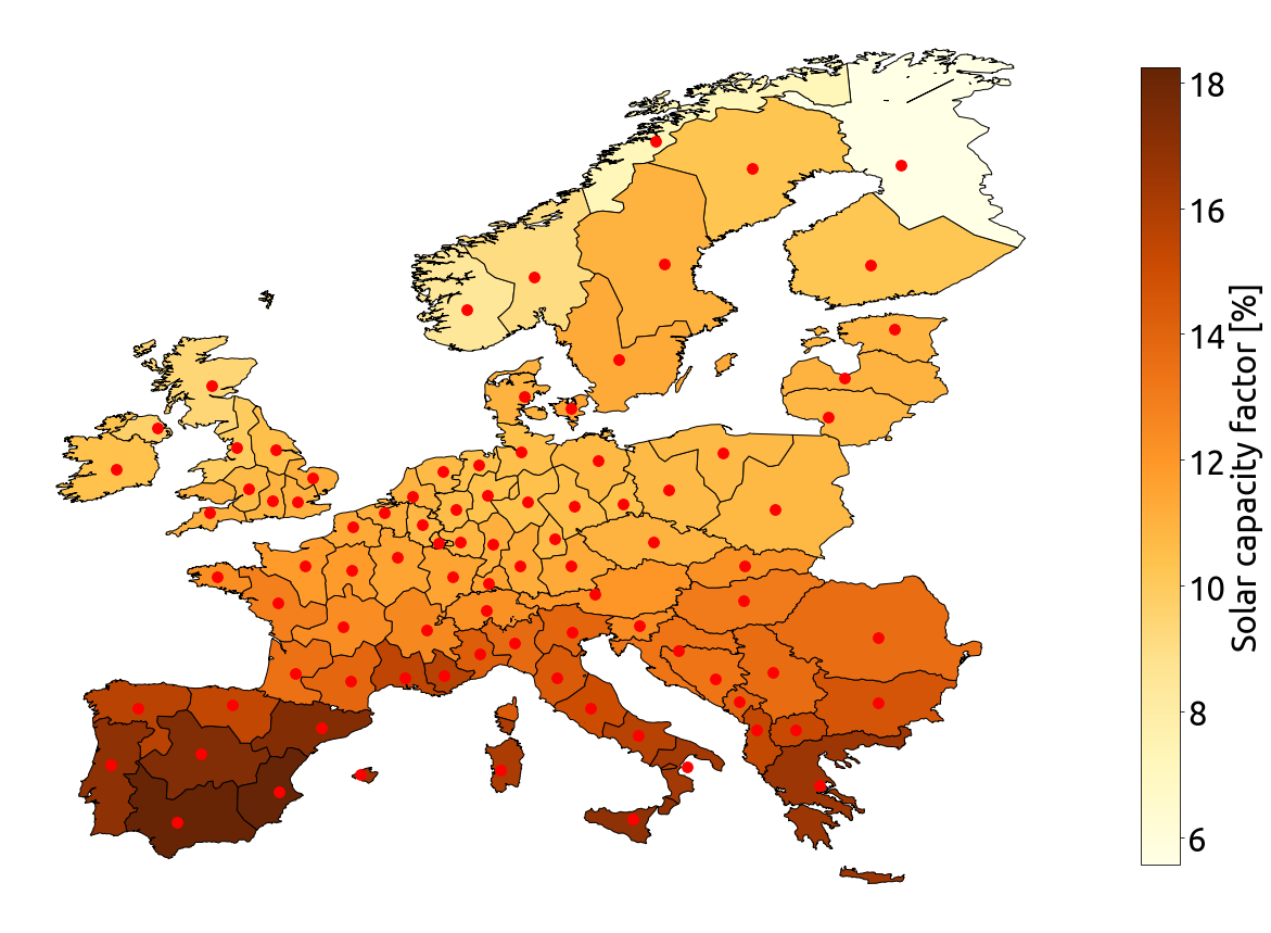
(b)

Figure S9: (a) Onshore wind capacity factors across Europe and (b) Solar photovoltaic capacity factors across Europe. The capacity factors for wind are predominantly higher in northern Europe, whereas the capacity factors for solar are predominantly higher in southern Europe.

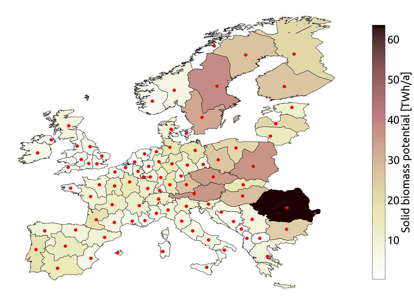
(a)

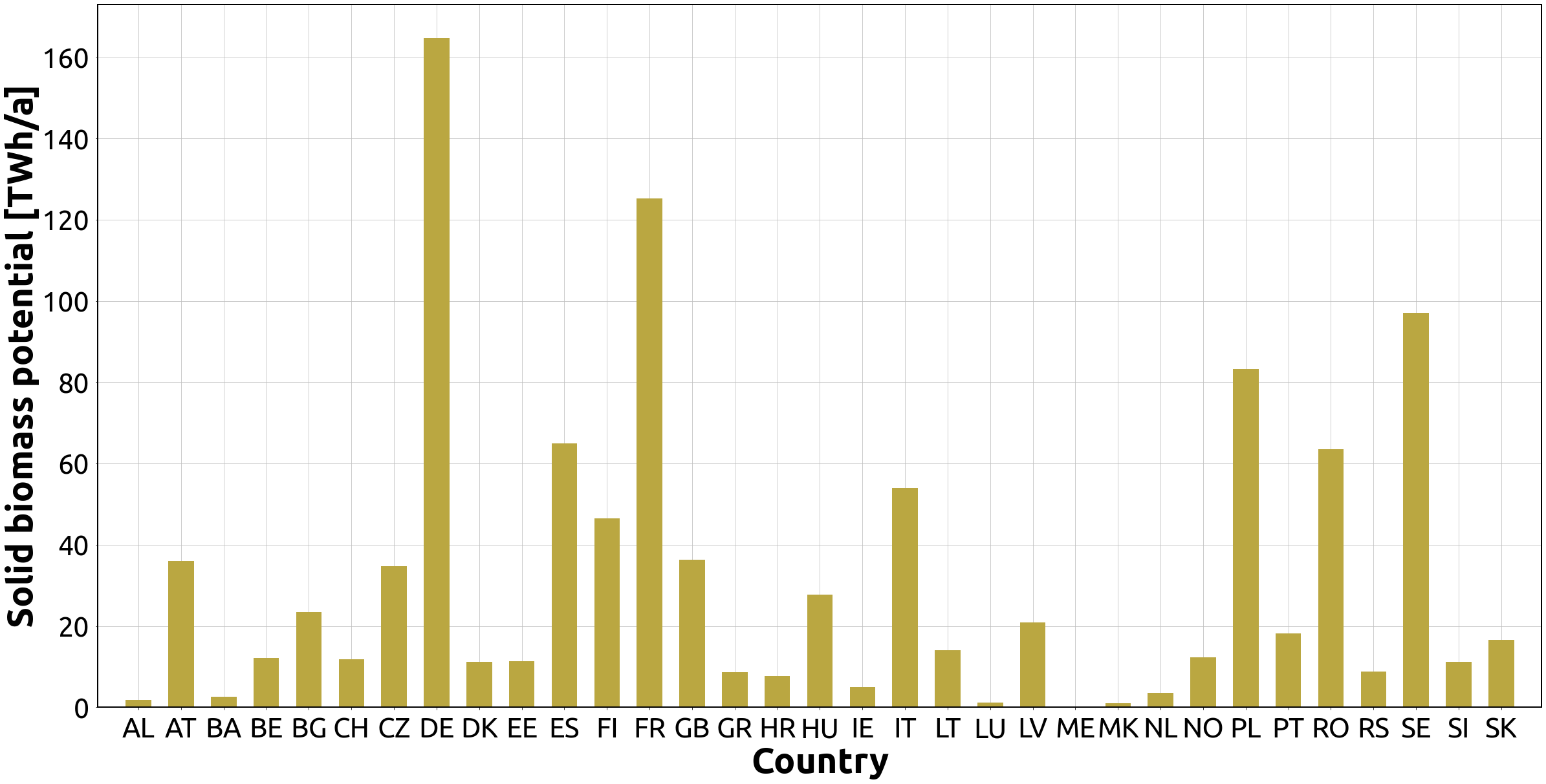
(b)

Figure S10: Solid biomass potential (a) per node and (b) per country. Europe is assumed to have an aggregated potential of 1038 TWh per year of solid biomass. This assumption is based on the medium bioenergy availability profile of the ENSPRESO database, which the model uses in both the global and local net-zero CO₂ emissions scenarios.

Under a global net-zero CO₂ emissions constraint, we see non-uniform results, with several countries emitting more CO₂ than they capture on average throughout the year, resulting in a total net emission of 195 MtCO₂. Specifically, Germany, Belgium, and the Netherlands (hereafter referred to as “interior countries”) are responsible for 85% of this total. In contrast, net absorbers such as Spain, Sweden, Finland, Poland, and Romania (hereafter referred to as “exterior countries”) are collectively responsible for absorbing 66% of the total net emission. See Figures 1 and S6. The lack of uniformity stems from the variation in European nations’ CO₂ process emissions, energy-related emissions from the industry, and emissions from the agriculture, shipping and aviation sectors (Figure S7), their different potential to sequester CO₂ underground (Figure S8), distinct access to renewable resources such as wind and solar (Figure S9) for powering, e.g., DAC, and differing solid biomass resources (Figure S10).

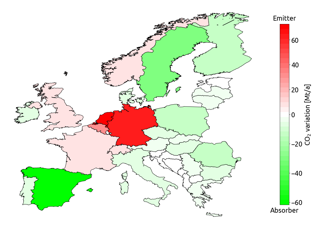
Figure 1: Net CO₂ emitter and absorber countries in the global net-zero CO₂ emissions scenario. Countries capturing more CO₂ than they emit on a yearly average are shown in green, while countries capturing less CO₂ than they emit are shown in red.

In a locally constrained scenario, the exchange of CO₂ with the atmosphere is net-zero at every country. However, a country can still exchange CO₂ with neighbouring countries in various ways. This can be accomplished either directly through underground CO₂ pipelines (built by the model if cost-effective) or indirectly through the exchange of synthetic oil, methane gas, and methanol, all of them produced by combining electrolytic H₂ and captured CO₂ when economically beneficial. Another way to indirectly exchange CO₂ is by transporting solid biomass amongst countries.

In the following sections, we will investigate the major changes in costs, CO₂ capture, transportation, conversion, and sequestration levels across Europe, as well as their operational patterns over time, when comparing a scenario with a global net-zero CO₂ emissions target versus one with local net-zero CO₂ emissions targets.

2.1 System cost and technology configuration

In a global net-zero CO₂ emissions scenario, the major contributors to the total system cost (878 billion € per year) include wind and solar photovoltaic (PV) capacities, technologies to electrify the heating sector, and the production of electrolytic H₂. These are also the main contributors to the total cost of a system under local net-zero CO₂ emissions scenario, which suffers a 1.4% increase relative to the system under a global constraint. See Figure 2. The increase is mainly due to an expansion in the capacity of DAC and solar PV, especially in the interior countries (Figures 3 and S16), along with higher usage of air heat pumps and biomass boilers. It is important to note that, while certain technologies increase the total system cost, others decrease it by becoming less relevant under local constraints. These include the reduction of solar thermal and carbon capture from solid biomass-based CHP units in many net CO₂ absorber countries since their need to capture CO₂ is relaxed. Furthermore, we found that a climate-neutral energy system under nodal constraints, where each of the 90 nodes is set with a net-zero CO₂ emissions target (Equation S5), is 1.7% more expensive than when under a global constraint. This demonstrates that even in a more restrictive scenario like the nodal-constrained one, achieving a socially fairer energy system in Europe is feasible with only a slight cost increase compared to the global scenario.

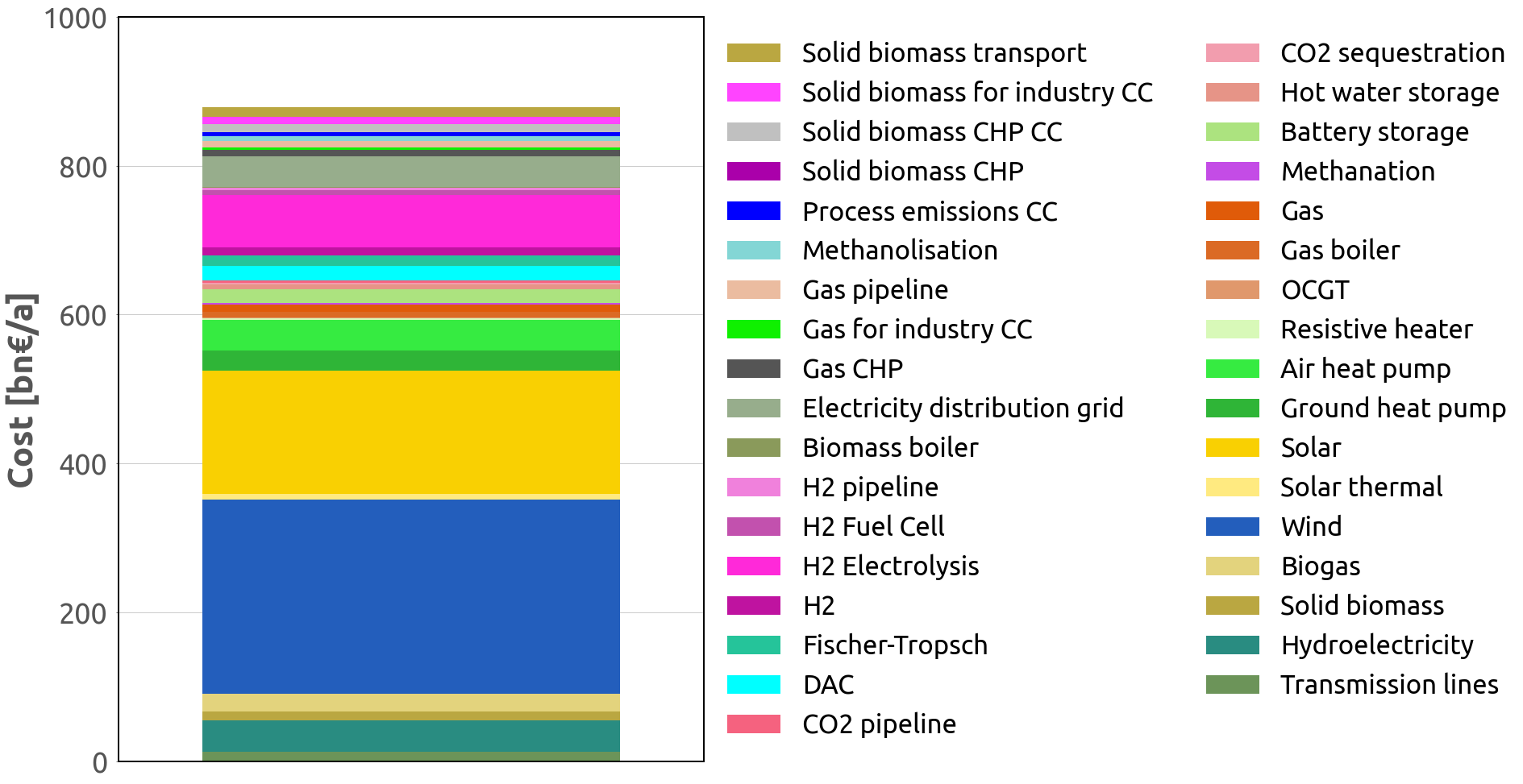
(a)

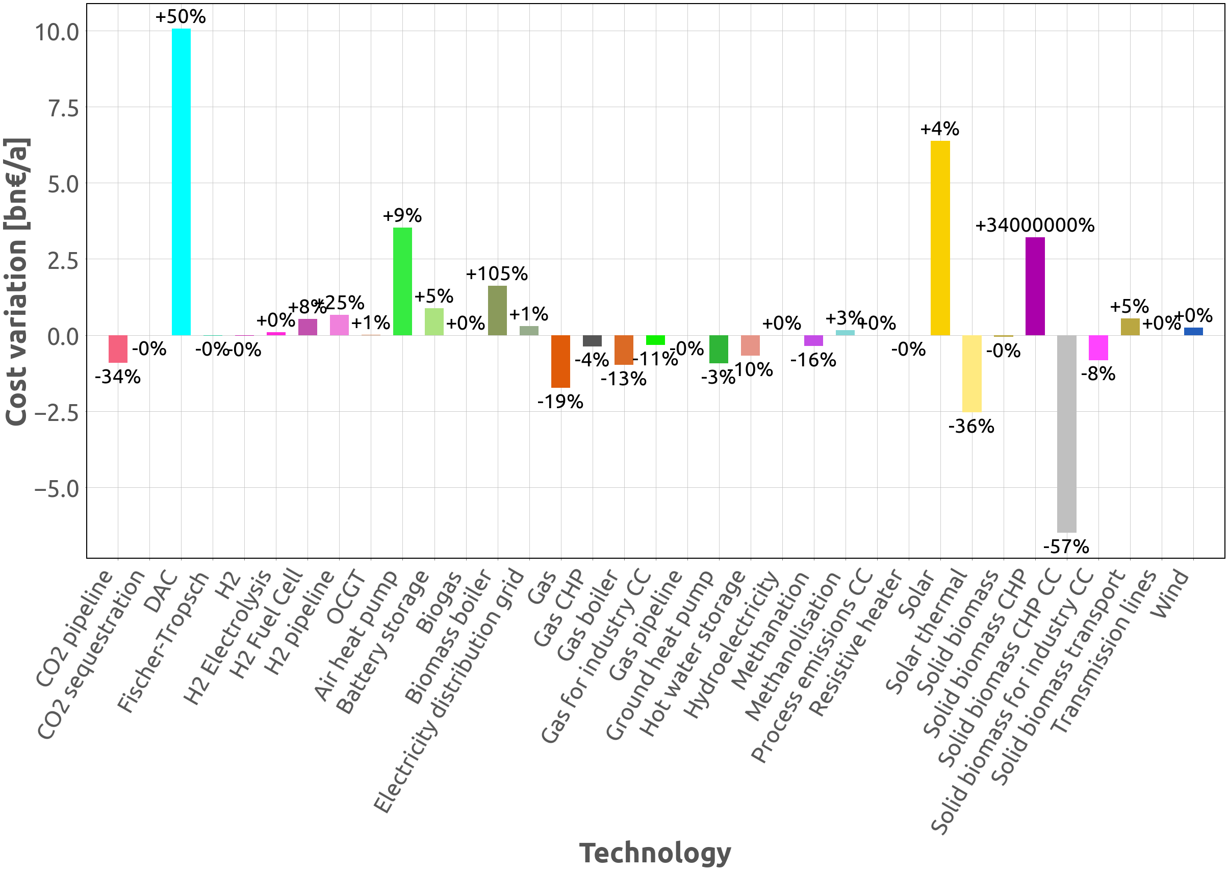
(b)

Figure 2: (a) Total system cost and technology configuration in the global net-zero CO₂ emissions scenario and (b) Cost variation per technology between the global net-zero CO₂ emissions scenario and the local net-zero CO₂ emissions scenario.

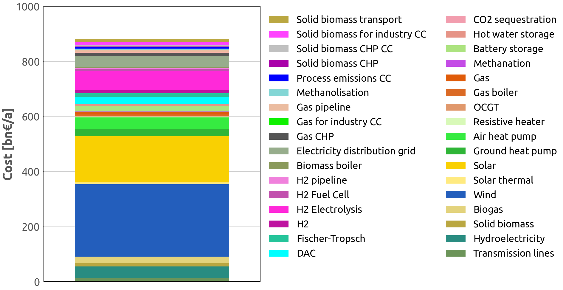
(a)

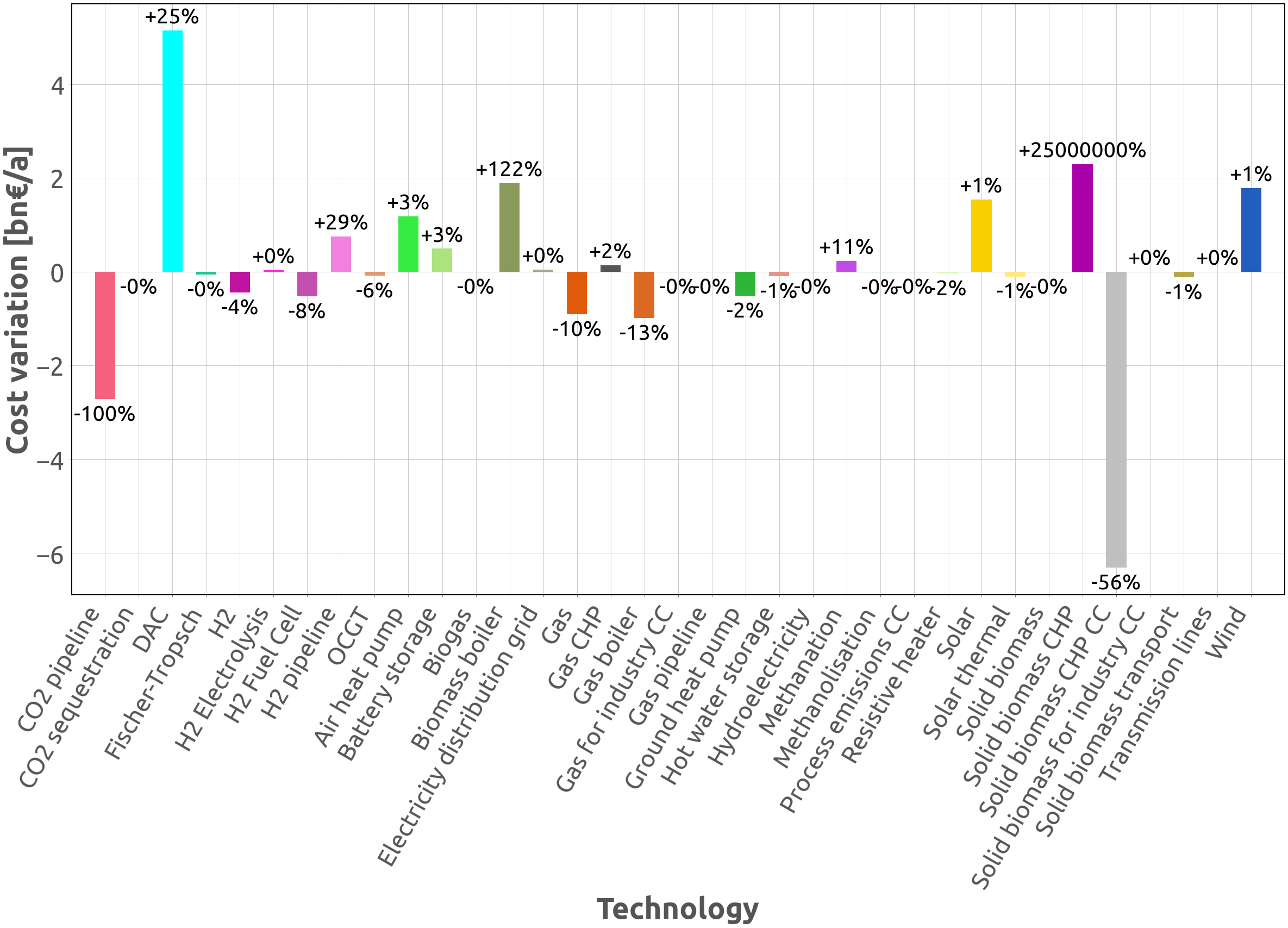
(b)

Figure S14: (a) Total system cost and technology configuration in the global net-zero CO₂ emissions scenario without a CO₂ network and (b) Cost variation per technology between the global net-zero CO₂ emissions scenario with a CO₂ network and the global net-zero CO₂ emissions scenario without a CO₂ network. The total cost increases by 0.3% when modelling a system without a CO₂ network compared to its counterpart equipped with such a network. Other than the differences in deployment levels, the technology configuration is the same in both types of systems.

In case Europe does not establish a CO₂ network amongst its nations, the model predicts that a climate-neutral energy system would experience a 0.3% cost increase (2.6 billion € per year) in a globally constrained scenario and a 0.6% cost increase (5.4 billion € per year) in a locally constrained scenario, compared to their counterparts equipped with a CO₂ network (Figures S14 and S15). The cost increase is due to the model no longer leveraging from a network to manage captured CO₂ efficiently by sending it to neighbouring countries for underground sequestration or helping countries to balance their national CO₂ demand and supply for manufacturing synthetic products amongst themselves.

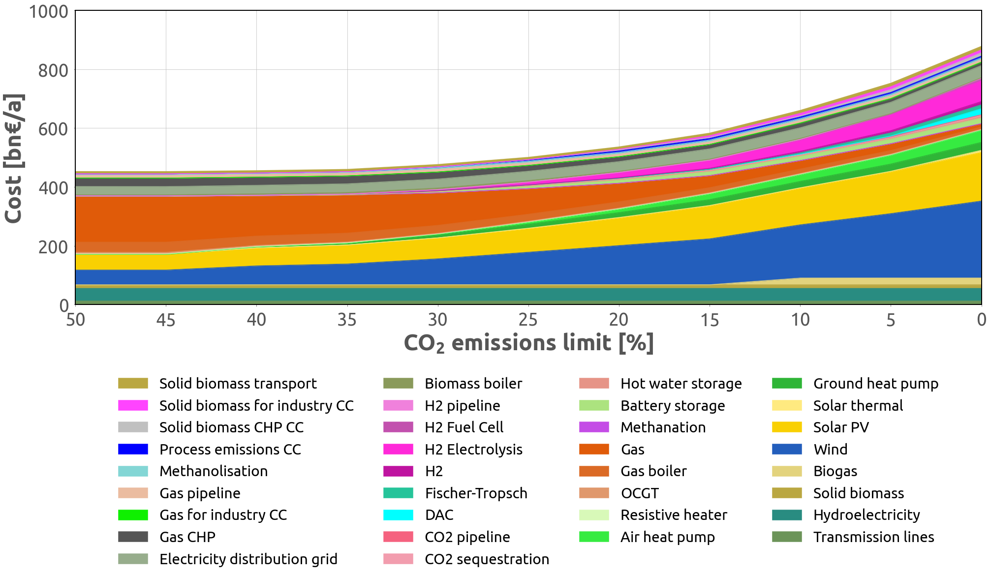
(a)

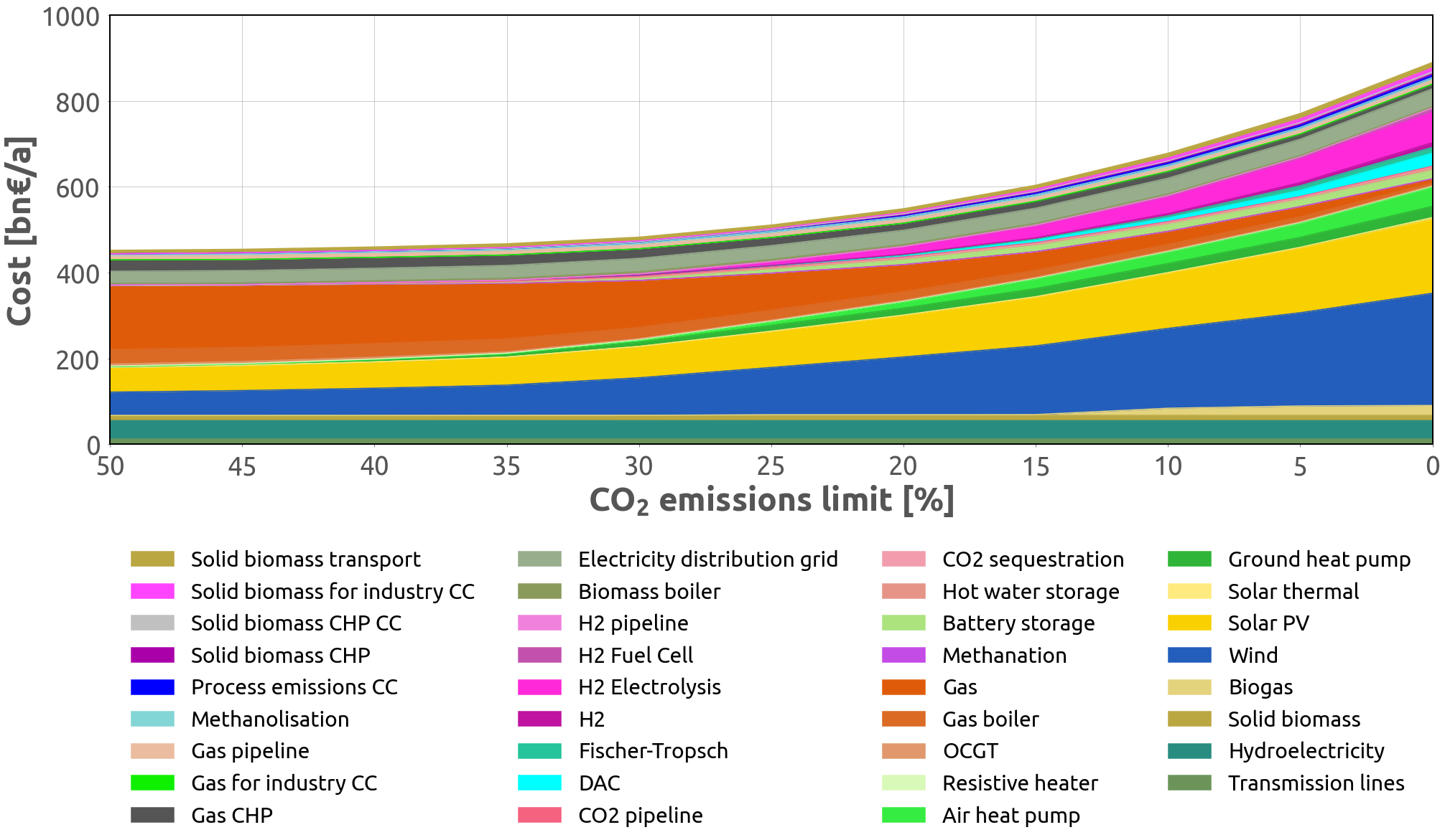
(b)

Figure S11: Total system cost sensitivity analysis under different CO₂ emissions limits and respective technology configuration in (a) the global scenario and (b) the local scenario. Until reaching a 35% limit in CO₂ emissions (relative to 1990 levels), the total system cost remains constant since the CO₂ constraint is not binding. After that point, the cost increases non-linearly in both scenarios until Europe is fully decarbonised.

As a next step, to understand better the impacts of the CO₂ constraints, we conducted a sensitivity analysis to assess how the model reacts under different CO₂ emissions limits in terms of cost and technology configuration (Figure S11). The results show that up to the point where CO₂ emissions are reduced to 35% of 1990 levels, the total system cost stays constant at 540 billion € per year in a globally constrained scenario and 548 billion € per year in a locally constrained scenario. After this point, reducing emissions further increases costs non-linearly in both scenarios until the continent is fully decarbonised. Furthermore, as the limit becomes stricter, the model gradually shifts from using methane gas to renewable technologies and technologies for direct and indirect electrification. Despite variations in deployment levels, the technologies composing each of the modelled scenarios remain the same, regardless of the imposed CO₂ emissions limit.

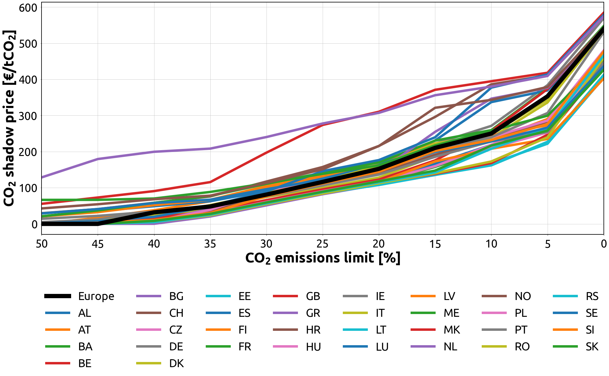
(a)

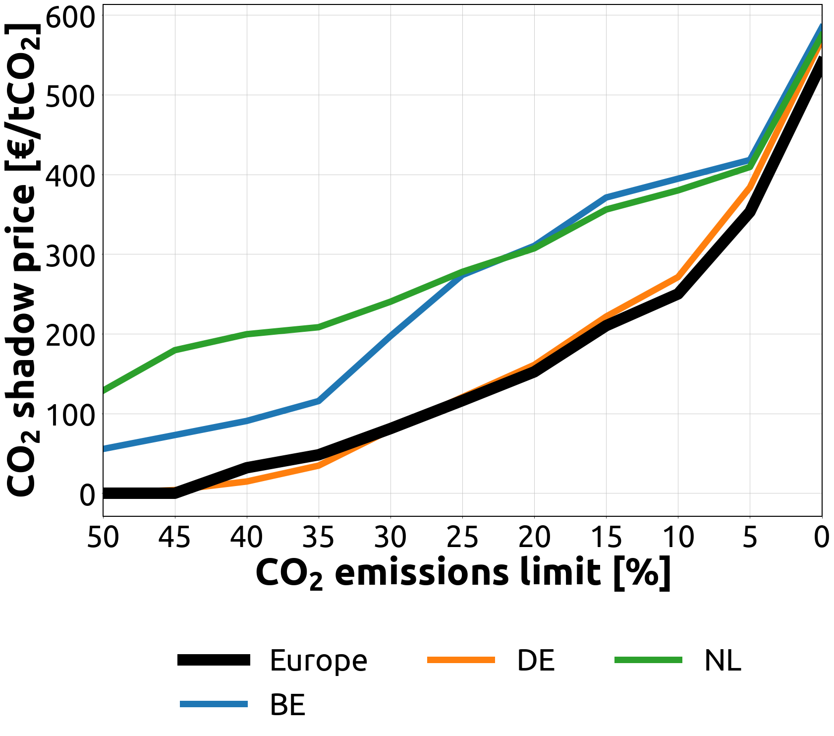
(b)

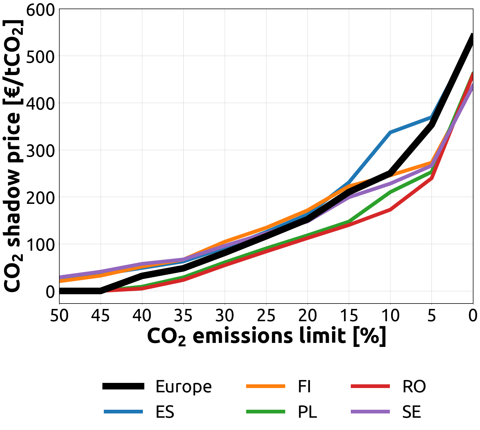
(c)

Figure S12: CO₂ shadow price sensitivity analysis under different CO₂ emissions limits (a) for Europe (global scenario) and all the modelled countries (local scenario), (b) for Europe (global scenario) and the interior countries (local scenario), and (c) for Europe (global scenario) and the exterior countries (local scenario). In a continent fully decarbonised under local constraints, countries that used to emit more CO₂ than they absorb annually in the global scenario have local CO₂ shadow prices higher than Europe’s global CO₂ shadow price. Conversely, countries that used to absorb more CO₂ than they emit in the global scenario have local CO₂ shadow prices lower than Europe’s global CO₂ shadow price.

The required CO₂ price to attain the emissions target is an output of the model. For the global net-zero emissions constraint, it resulted in 540 €/tCO₂. On the other hand, when local net-zero emissions constraints are imposed, the price required to attain climate neutrality in Europe as a whole varies significantly across countries, ranging from 402 in Latvia to 584 €/tCO₂ in Belgium (Figures S12 and S13 and Table S4). The variation is due to each country having a distinct mix of sources and amounts of CO₂ emissions, as well as renewable energy resources. As expected, there is a pattern between the price and whether countries are net CO₂ emitters or absorbers: emitting countries have higher local prices than the global CO₂ shadow price, whereas absorbing countries have lower local prices than the global CO₂ shadow price.

2.2 Carbon capture

In the model, CO₂ is primarily captured from: (i) industry process emissions, (ii) gas and solid biomass used for heating in the industry and combusted in CHP units, and (iii) DAC. On a continental level, both climate-neutral scenarios result in a similar total of 724 MtCO₂ emitted and captured annually by these methods. However, at a national level, the amount of CO₂ captured and the methods used show significant variations between the two scenarios (Figure 3).

The first remarkable change is how DAC shifts from net CO₂ absorber countries to net CO₂ emitter countries. The former countries have better access to renewable resources but, under local constraints, do not have such a strong push for capturing CO₂, which is transmitted to the latter countries. These install DAC in areas where district heating is available, which gives access to low-cost heat, increasing the competitiveness of DAC.

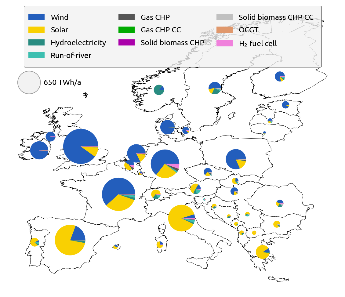
(a)

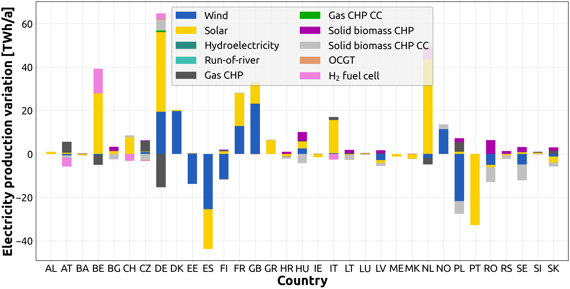
(b)

Figure S16: (a) Electricity production in the global net-zero CO₂ emissions scenario and (b) Electricity production variation per country and technology between the global net-zero CO₂ emissions scenario and the local net-zero CO₂ emissions scenario. Major variations occur in electricity production from renewable sources. While net CO₂ emitter countries increase solar and wind to produce electricity, net CO₂ absorber countries, on the other hand, decrease these. This is because the former countries capture much more CO₂ under local constraints using DAC and convert it into methanol, both processes requiring significant amounts of power, while the latter countries relax these (since they have to handle less captured CO₂).

Solid biomass-based CHP units with CC decline in most net CO₂ absorber countries under local constraints (Figure S16). In some countries, they are replaced by units without CC to cut costs. In others, they are not replaced since power and heating demand has reduced as a consequence of a reduction in DAC and methanol production (Figure 4), both of which are power-intensive processes, and an increase in air heat pumps (Figure 2(b)). CO₂ captured from solid biomass used in the industry also decreases due to no longer being cost-effective under these constraints.

The process emissions and the gas demand in the industry are exogenously fixed, and the model shows that capturing CO₂ from both sources is cost-effective in nearly every location, with minimal variation between the two scenarios. The production of blue H₂ is not cost-competitive in any region or scenario, and as a result, no CO₂ is captured from SMR.

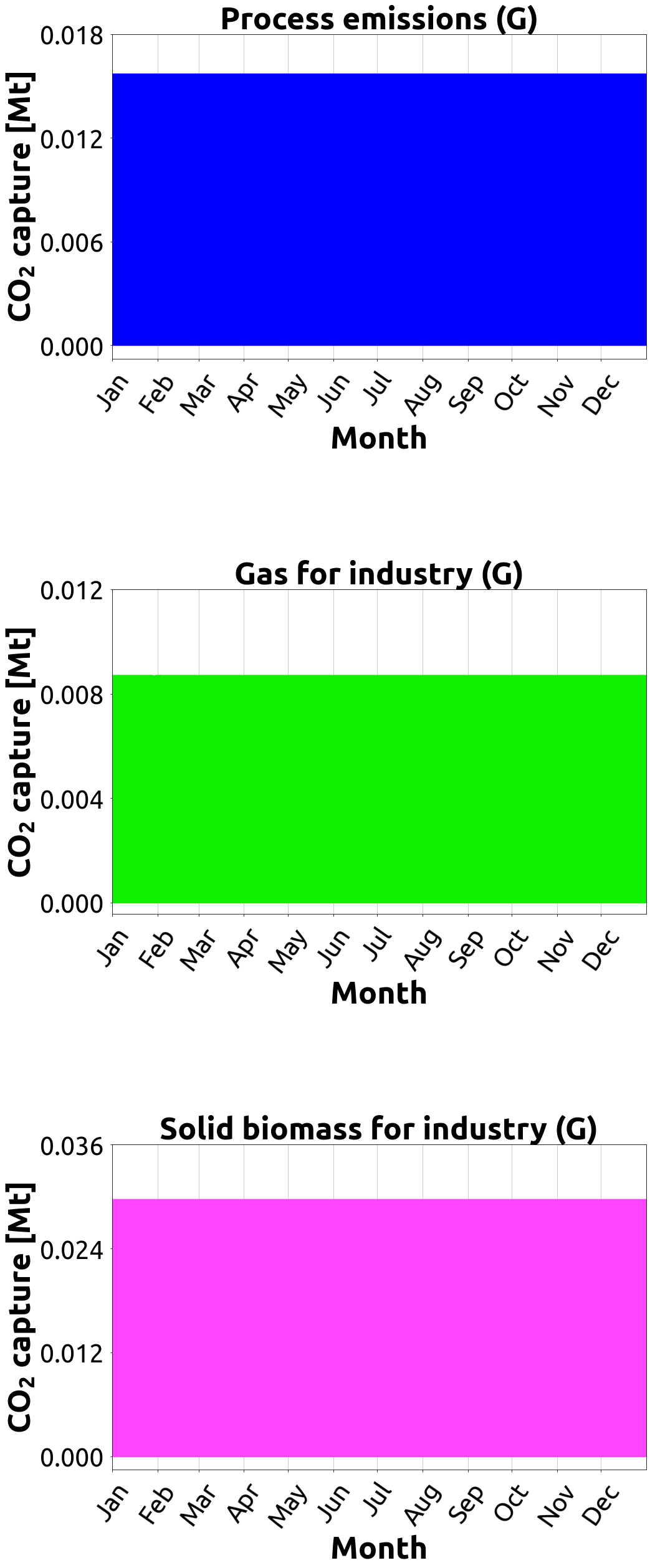
(a)

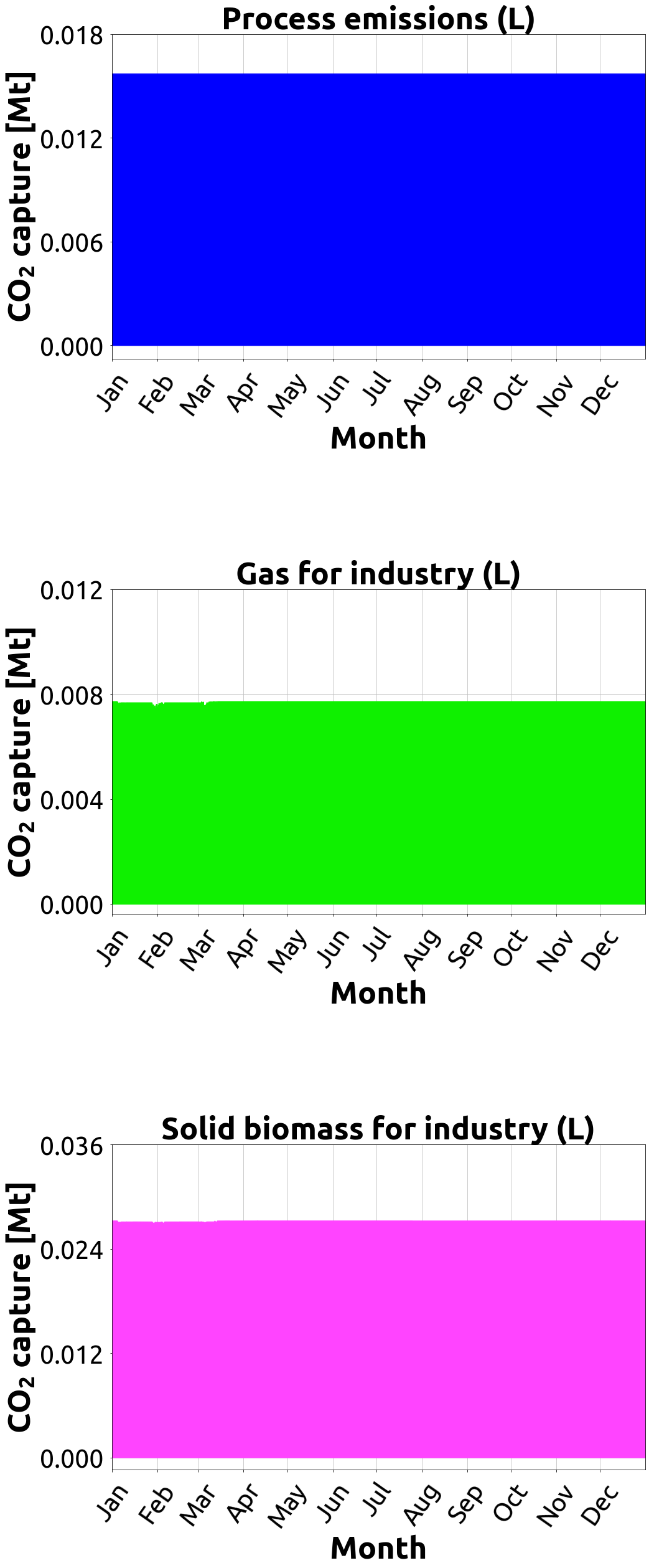
(b)

Figure S22: Temporal CO₂ capture from exogenously fixed sources across all of Europe in (a) the global net-zero CO₂ emissions scenario and (b) the local net-zero CO₂ emissions scenario.

From a temporal perspective, our results show two distinct operational patterns for capturing CO₂, present in both scenarios. The first pattern occurs when low-cost electricity is available, typically during the summer, to power DAC. The second pattern occurs when gas and solid biomass are combusted in CHP units to provide heat and power during the winter, using CC. Since industry is assumed to operate in continuous mode, the amount of CO₂ captured from process emissions, as well as gas and solid biomass used in the industry is kept constant throughout the year. See Figures S22 and S23.

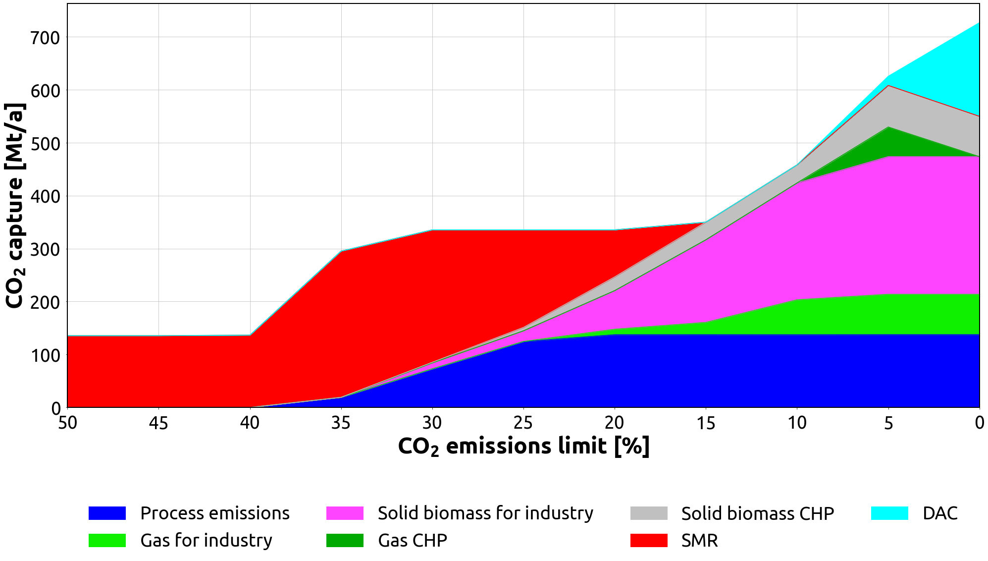
(a)

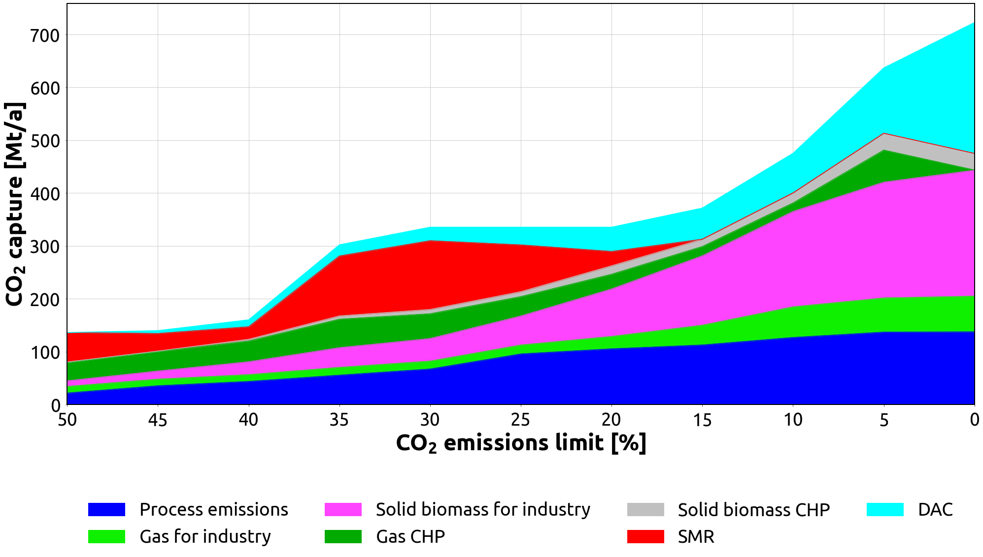
(b)

Figure S17: CO₂ capture sensitivity analysis under different CO₂ emissions limits in (a) the global scenario and (b) the local scenario. In the local scenario, CO₂ captured from DAC and solid biomass used in the industry are adopted for less stringent CO₂ targets in the CO₂ reduction path compared to the global scenario. In a fully decarbonised Europe, these two technologies combined account for 60% and 67% of the total CO₂ captured in the global and local scenarios, respectively.

When investigating the sensitivity to different CO₂ emissions targets (1990 levels), DAC is adopted at a less stringent CO₂ emissions limit (45%) in a local scenario compared to a global scenario (5%). Along with CO₂ captured from solid biomass used in the industry, which is also adopted at a less stringent limit (50%), they capture the bulk of CO₂ emissions, reaching 60% and 67% in a global and local net-zero CO₂ emissions scenarios, respectively. Although SMR with CC plays a crucial role in both scenarios for low CO₂ emissions reduction targets, as well as gas-based CHP units with CC in a local scenario, they both gradually decrease CO₂ capture levels until they become irrelevant for climate-neutral scenarios. See Figure S17.

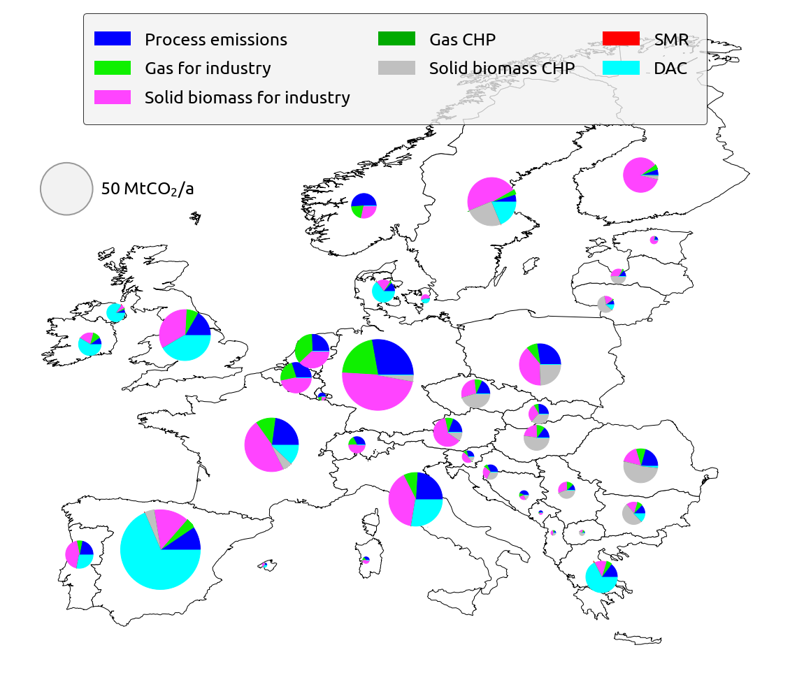
(a)

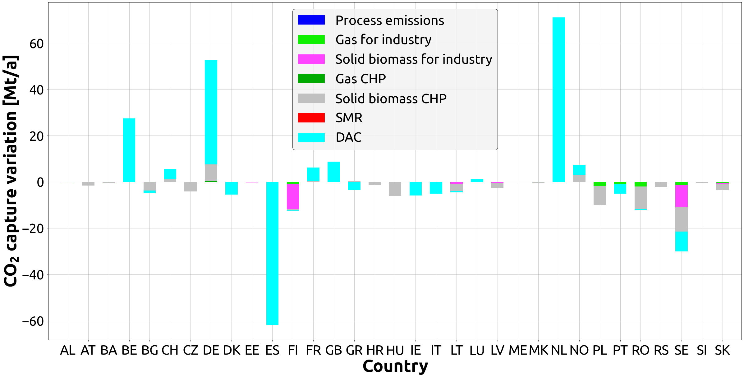
(b)

Figure 3: (a) CO₂ capture in the global net-zero CO₂ emissions scenario and (b) CO₂ capture variation per country and technology between the global net-zero CO₂ emissions scenario and the local net-zero CO₂ emissions scenario.

2.3 Carbon conversion and sequestration

In the model, captured CO₂ is either (i) utilised to produce carbonaceous fuels such as synthetic oil through the Fischer-Tropsch process, synthetic methanol in methanolisation plants, and synthetic methane through the Sabatier reaction, or (ii) sequestered underground. The total CO₂ converted and sequestered underground remains essentially the same in both climate-neutral scenarios, 724 Mt per year, at a continental level. However, the amount of converted CO₂ and the types of products it is converted into, as well as the levels of CO₂ sequestered underground vary significantly in each country between the two scenarios (see Figure 4).

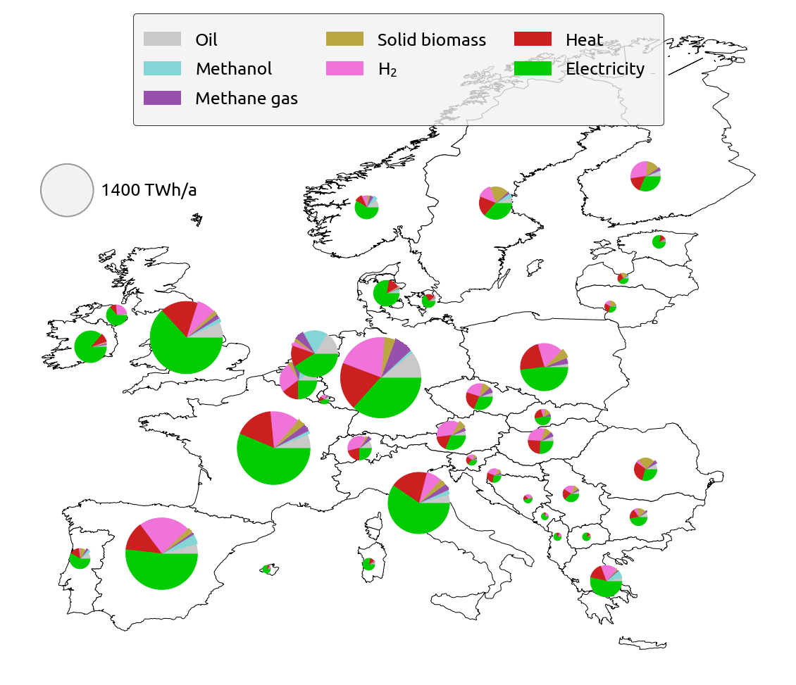
(a)

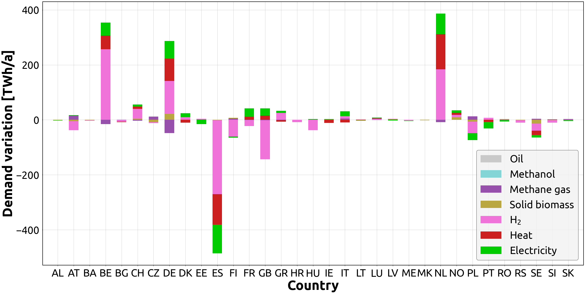
(b)

Figure S19: (a) Oil, methanol, methane gas, solid biomass, H₂, heat, and electricity demand in the global net-zero CO₂ emissions scenario and (b) Oil, methanol, methane gas, solid biomass, H₂, heat, and electricity demand variation per country between the global net-zero CO₂ emissions scenario and the local net-zero CO₂ emissions scenario. In the local scenario, the interior countries significantly increase the demand for H₂, heat, and electricity due to the growth in manufacturing synthetic products, along with the deployment of DAC and air heat pumps.

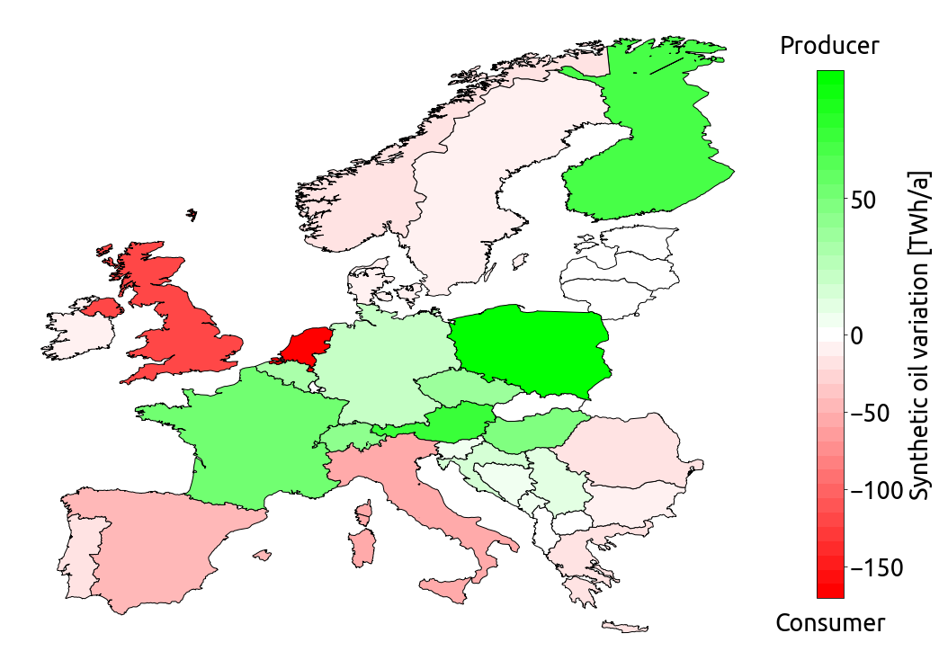
(a)

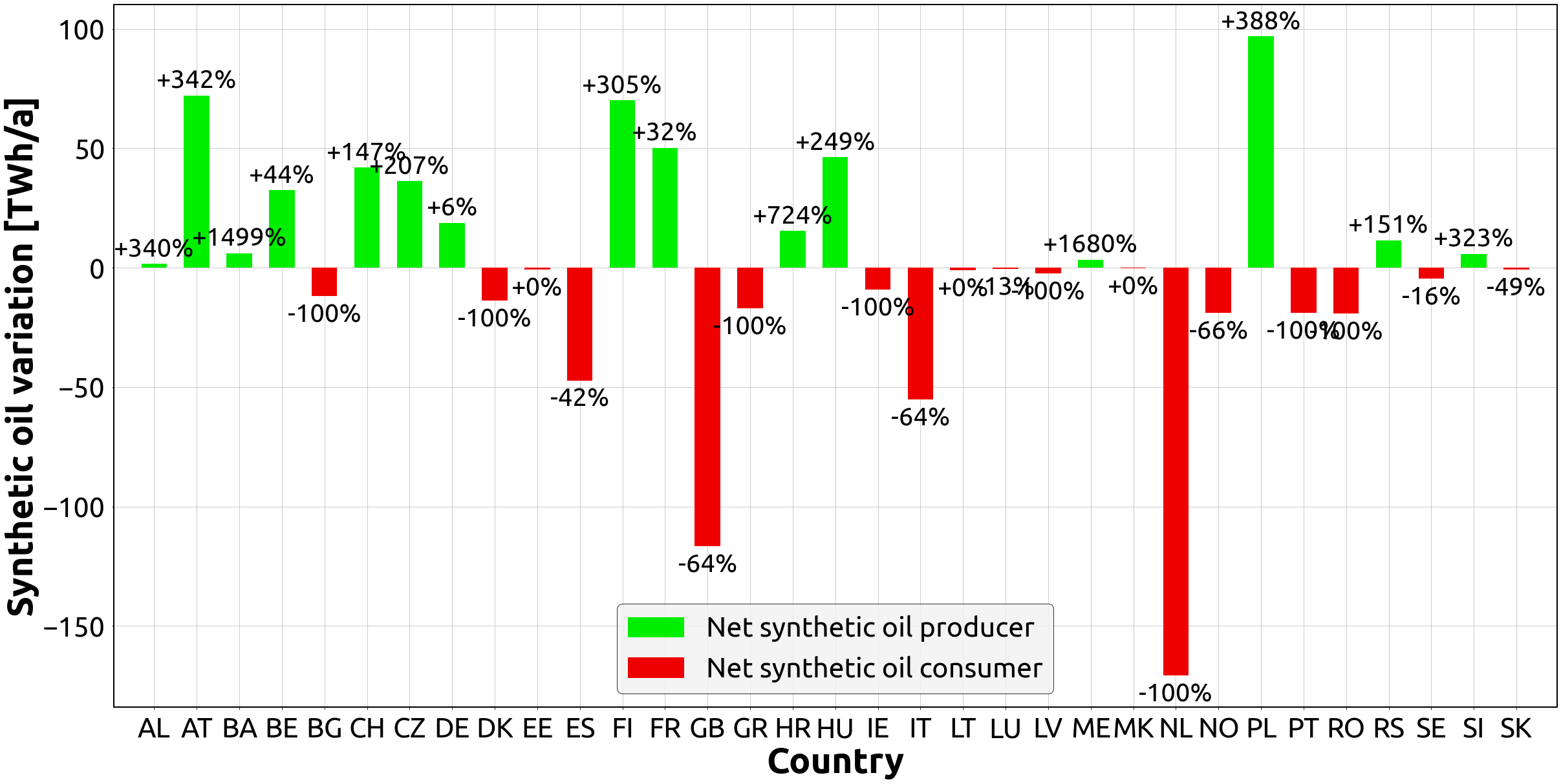
(b)

Figure S20: (a) Net synthetic oil producers and consumers in the global net-zero CO₂ emissions scenario and (b) Net synthetic oil variation per country in the global net-zero CO₂ emissions scenario. Countries that produce more synthetic oil than they consume are represented by green bars, while countries that consume more synthetic oil than they produce are represented by red bars. The percentages on top of the green bars indicate how much additional synthetic oil net producer countries manufacture, beyond what is needed to meet their own demand. On the other hand, the percentages at the bottom of the red bars indicate how much synthetic oil net consumer countries do not manufacture to meet their own demand, relying instead on the former countries.

Under local constraints, Belgium and Germany substantially increase synthetic oil production through the Fischer-Tropsch process to help meet climate targets (by reusing CO₂). This is to satisfy their high demand for this product (Figure S19), mainly in the industry and aviation sectors. In most net CO₂ absorber countries, synthetic oil production decreases given that they do not need to process as much captured CO₂ as they would in a globally constrained scenario (Figure S20).

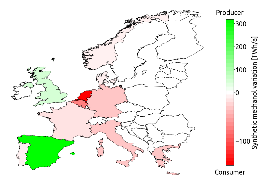
(a)

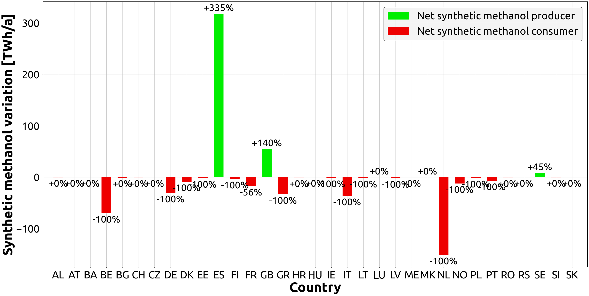
(b)

Figure S21: (a) Net synthetic methanol producers and consumers in the global net-zero CO₂ emissions scenario and (b) Net synthetic methanol variation per country in the global net-zero CO₂ emissions scenario. Countries that produce more synthetic methanol than they consume are represented by green bars, while countries that consume more synthetic methanol than they produce are represented by red bars. The percentages on top of the green bars indicate how much additional synthetic methanol net producer countries manufacture, beyond what is needed to meet their own demand. On the other hand, the percentages at the bottom of the red bars indicate how much synthetic methanol net consumer countries do not manufacture to meet their own demand, relying instead on the former countries.

We observe a substantial increase in synthetic methanol production in the interior countries under local constraints to meet the needs of their shipping sector, especially in the Netherlands. This is because they can no longer depend on Spain and Great Britain, two major producers of synthetic methanol (Figure S21), for the supply of this product as it occurs under a global constraint.

Regarding the production of synthetic methane gas through the Sabatier reaction, the model does not favour it in a global scenario and further reduces it in a local scenario. The high cost and high heat temperatures required by the process make it a challenging option in both scenarios. As a result, boilers consuming gas are replaced by solid biomass boilers and air heat pumps, which offer cleaner and cost-effective heating (Figure 2).

While in Germany and Great Britain (both net CO₂ emitters), much more CO₂ is sequestered underground, in Denmark, Ireland, Italy, Portugal, Latvia, and especially in Greece (all net CO₂ absorbers), there is a substantial decrease of CO₂ sequestered underground (Figures 4(b) and S8). This is because net emitter countries capture additional CO₂ under local constraints, forcing them to either sequester more CO₂ underground or convert more CO₂ into synthetic products. Conversely, net absorber countries capture less CO₂ mainly from DAC (Figure 3) and/or receive less CO₂ from neighbouring countries (Figure 5), thus are less inclined to sequester CO₂ underground. Most net CO₂ emitter countries, including the interior countries, do not show any changes in the amount of CO₂ sequestered underground, with their potentials being fully utilised in both scenarios. Furthermore, the maximum limit of 200 MtCO₂ that can be sequestered underground annually across Europe is fully exhausted in both scenarios.

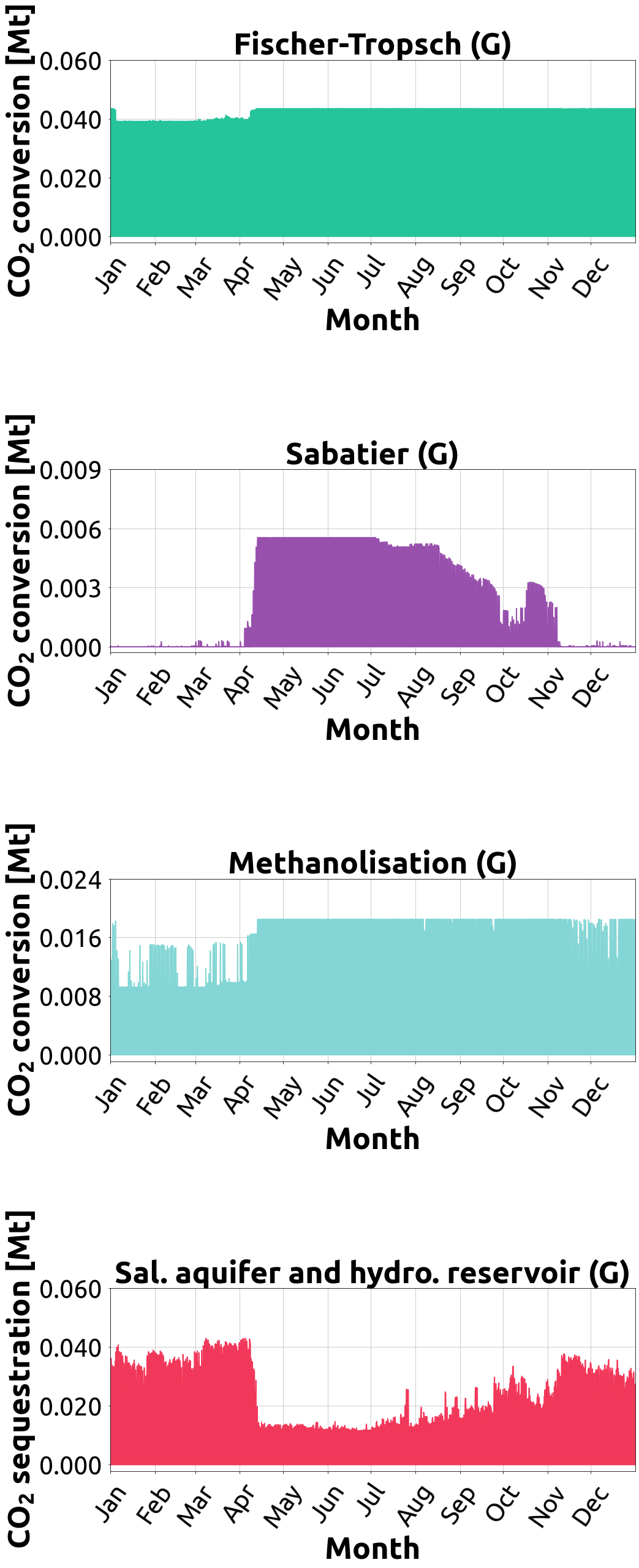
(a)

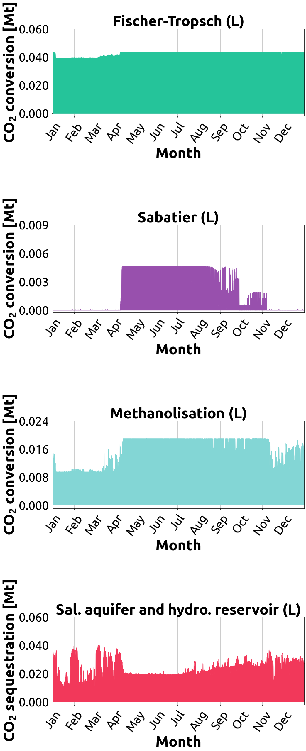
(b)

Figure S24: Temporal CO₂ conversion and sequestration across all of Europe in (a) the global net-zero CO₂ emissions scenario and (b) the local net-zero CO₂ emissions scenario. Although less prominent in Fischer-Tropsch, all CO₂ conversion processes exhibit a seasonal pattern. These processes convert more CO₂ during summer due to lower electricity and heating prices in this season and convert less during winter. Sequestration of CO₂ underground also follows a seasonal pattern, albeit inverted from the one governing the CO₂ conversion processes. During winter, more CO₂ is sequestered underground, while less is sequestered during summer due to its utilisation in conversion processes.

From a temporal perspective, our results show that both the Sabatier and the methanolisation processes exhibit a seasonal trend, whereas the Fischer-Tropsch process remains almost constant in the two modelled scenarios. The reason for this is that Fischer-Tropsch has high investment cost. Once the model selects it, the process typically operates at full capacity to recover costs. On the other hand, both Sabatier and methanolisation have lower investment costs that can operate flexibly, usually during periods of low electricity prices. Thanks to affordable electricity in the summer, which is essential for powering DAC to capture and provide the necessary CO₂ for all the conversion processes, as well as for powering the methanolisation process itself, the production of synthetic methane gas and methanol naturally increases during that season and decreases during the winter. Sequestering CO₂ underground also exhibits a seasonal trend in both scenarios, but it is opposite to the first two conversion processes mentioned earlier, with the model using this method more to deal with CO₂ during winter and less during summer. This is because CO₂ is needed to manufacture synthetic products during the summer, which reduces the amount of CO₂ sequestered underground in this period. See Figure S24.

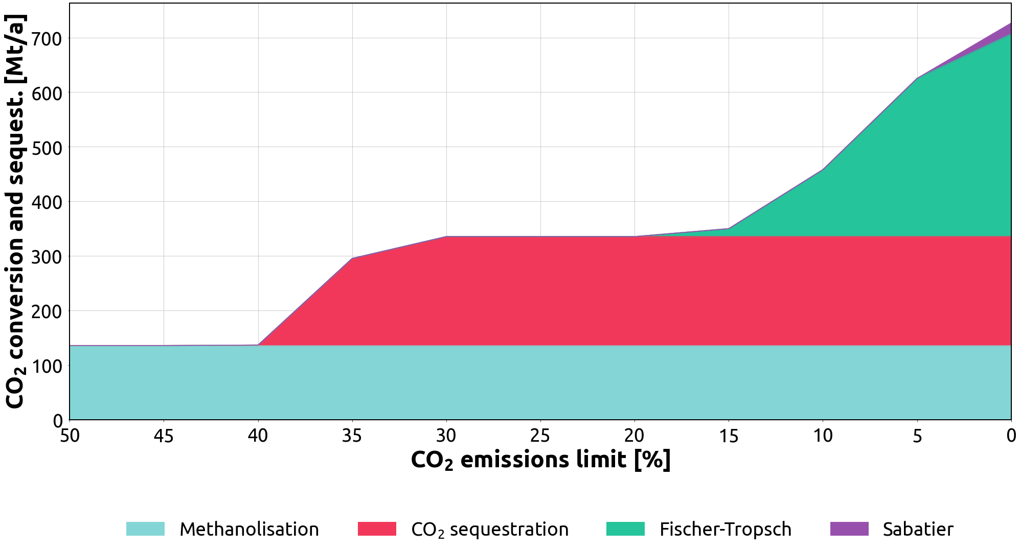
(a)

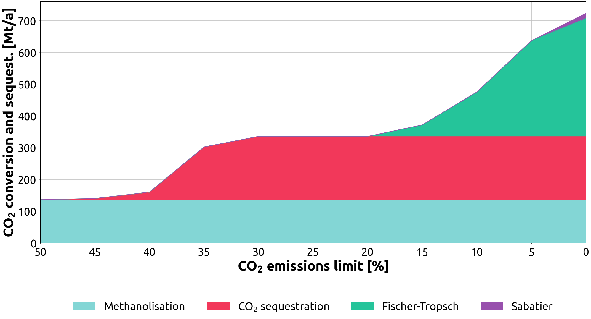
(b)

Figure S18: CO₂ conversion and sequestration sensitivity analysis under different CO₂ emissions limits in (a) the global scenario and (b) the local scenario. In both scenarios, Fischer-Tropsch and methanolisation play an important role in a fully decarbonised Europe by converting 70% of all captured CO₂ into synthetic oil and methanol. The remaining captured CO₂ is sequestered underground to enable negative emissions. As expected, the CO₂ conversion and sequestration profile mimics the CO₂ capture profile in both scenarios.

When investigating the sensitivity to different CO₂ emissions targets (1990 levels), methanolisation is constantly used in both scenarios since it is the only option to supply the exogenous methanol demand. Sequestering captured CO₂ underground in saline aquifers and hydrocarbon reservoirs starts at 40% and 45% of the CO₂ emissions limits in global and local scenarios, respectively. This allows for sequestering emissions from various industry processes, as well as enabling negative emissions. Fischer-Tropsch, which is adopted at a more stringent target (20% CO₂ emissions limit in both scenarios), deals with the remaining captured CO₂ by converting it into synthetic oil. See Figure S18.

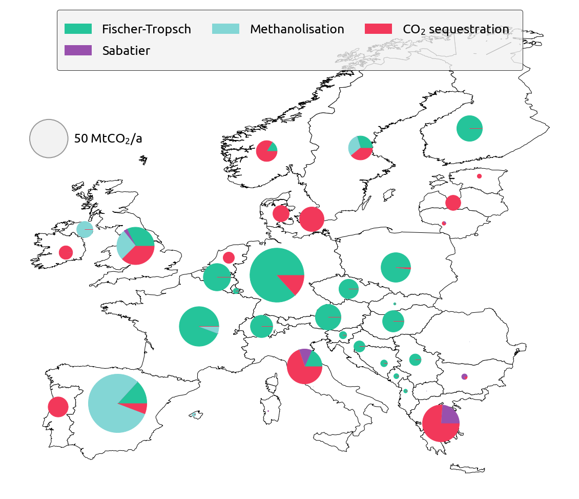
(a)

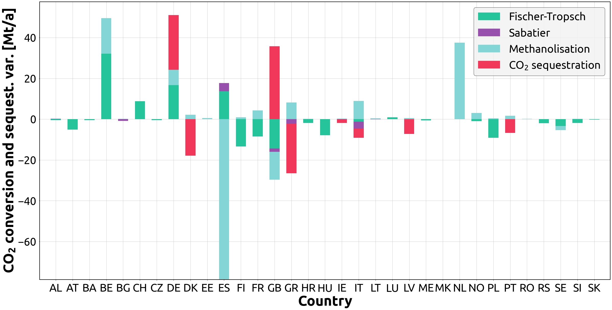
(b)

Figure 4: (a) CO₂ conversion and sequestration in the global net-zero CO₂ emissions scenario and (b) CO₂ conversion and sequestration variation per country and technology between the global net-zero CO₂ emissions scenario and the local net-zero CO₂ emissions scenario.

2.4 Carbon flow

We shift our attention now to investigating the flows of carbon in the model. This involves analysing the flows of CO₂ through newly built pipelines but also the flows of energy carriers that contain carbon such as methane gas and solid biomass. The analysis also considers the flows of electricity to help understanding where countries obtain the electricity needed for their CO₂ capture and conversion activities, as well as the flows of H₂ (through the modelled hydrogen network), considering the impact that changes in the locations where synthetic products are manufactured might have on these flows.

In a global and local net-zero CO₂ emissions scenarios, 124 GtCO₂·km/a and 87 GtCO₂·km/a are transported amongst and within countries through pipelines, respectively (Figure 5). Given that the total captured CO₂ amounts to 724 MtCO₂/a, transporting 124 GtCO₂·km/a can be interpreted as if, on average, 124 MtCO₂/a (17% of the captured CO₂) are transported 1000 km.

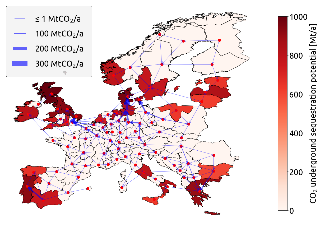
(a)

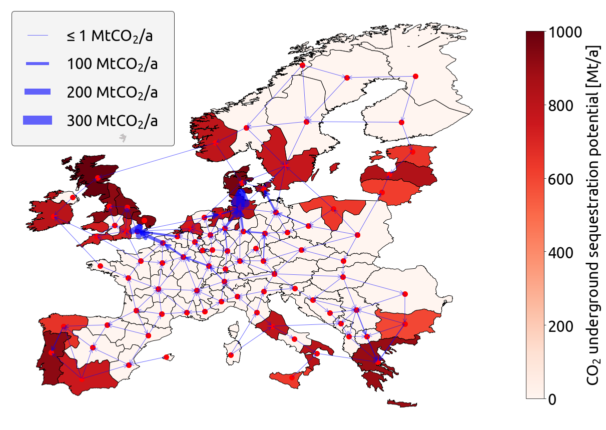
(b)

Figure S25: CO₂ flow with a 1000 Mt/a underground sequestration potential in (a) the global net-zero CO₂ emissions scenario and (b) the local net-zero CO₂ emissions scenario. The main factor determining the directions and destinations of CO₂ flows is the assumed potential for sequestering CO₂ underground. Increasing the potential assumption to 1000 Mt/a (from 200 Mt/a) across Europe clearly shows CO₂ flows converging towards countries with significant underground sequestration potential.

In both scenarios, the main factor determining the directions and destinations of flows is the assumed potential for sequestering CO₂ underground. As illustrated in Figure S25, increasing the potential assumption to 1000 MtCO₂/a (from 200 MtCO₂/a) across Europe clearly shows CO₂ flows converging towards countries with significant underground sequestration potential, such as Great Britain, Denmark, Portugal, Latvia, and Greece. This is in line with the results found in [11].

Comparing both scenarios, we observe a 30% (37 GtCO₂·km/a) decrease in the flow of CO₂ in a local scenario. This is mainly justified by Sweden and Romania, both important net absorbers under a global constraint, capturing less CO₂ under local constraints. As a result, these countries send less CO₂ to Denmark and Greece (via Bulgaria) for underground sequestration, respectively, considering their significant storage capacity (Figure S8). On the other hand, the Netherlands, the most important net emitter under a global constraint, captures much more CO₂ under local constraints (Figure 3). After using its captured CO₂ to produce additional synthetic methanol to meet the demand (Figure 4), the Netherlands starts sending excess CO₂ to Germany and Belgium. In turn, Germany sequesters the received CO₂ underground and Belgium uses it to produce additional synthetic oil and methanol required by local constraints. In addition, northeastern Germany starts sending CO₂ to Denmark for underground sequestration. The rise of CO₂ flow triggered by the Netherlands and Germany does not offset the previously described decrease in flow though, resulting in an overall 30% reduction in CO₂ flow, as mentioned.

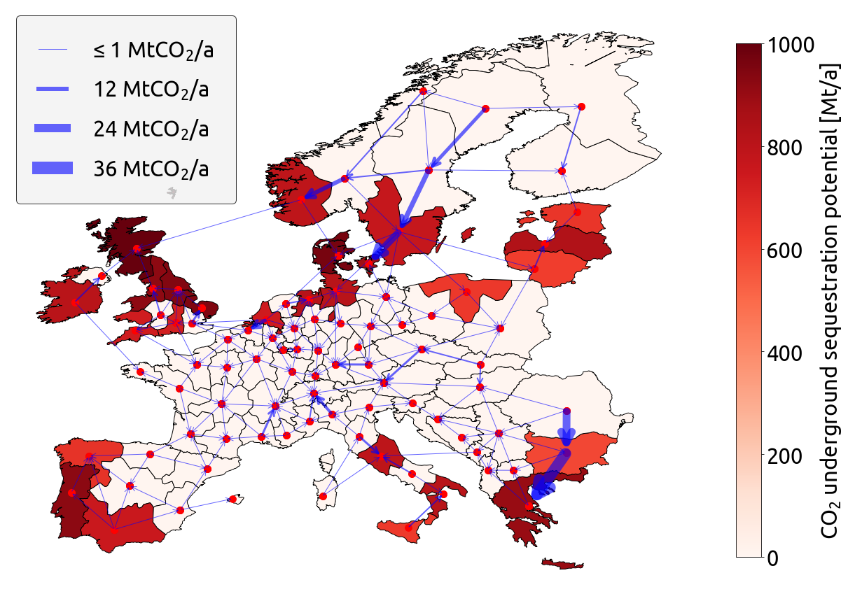
(a)

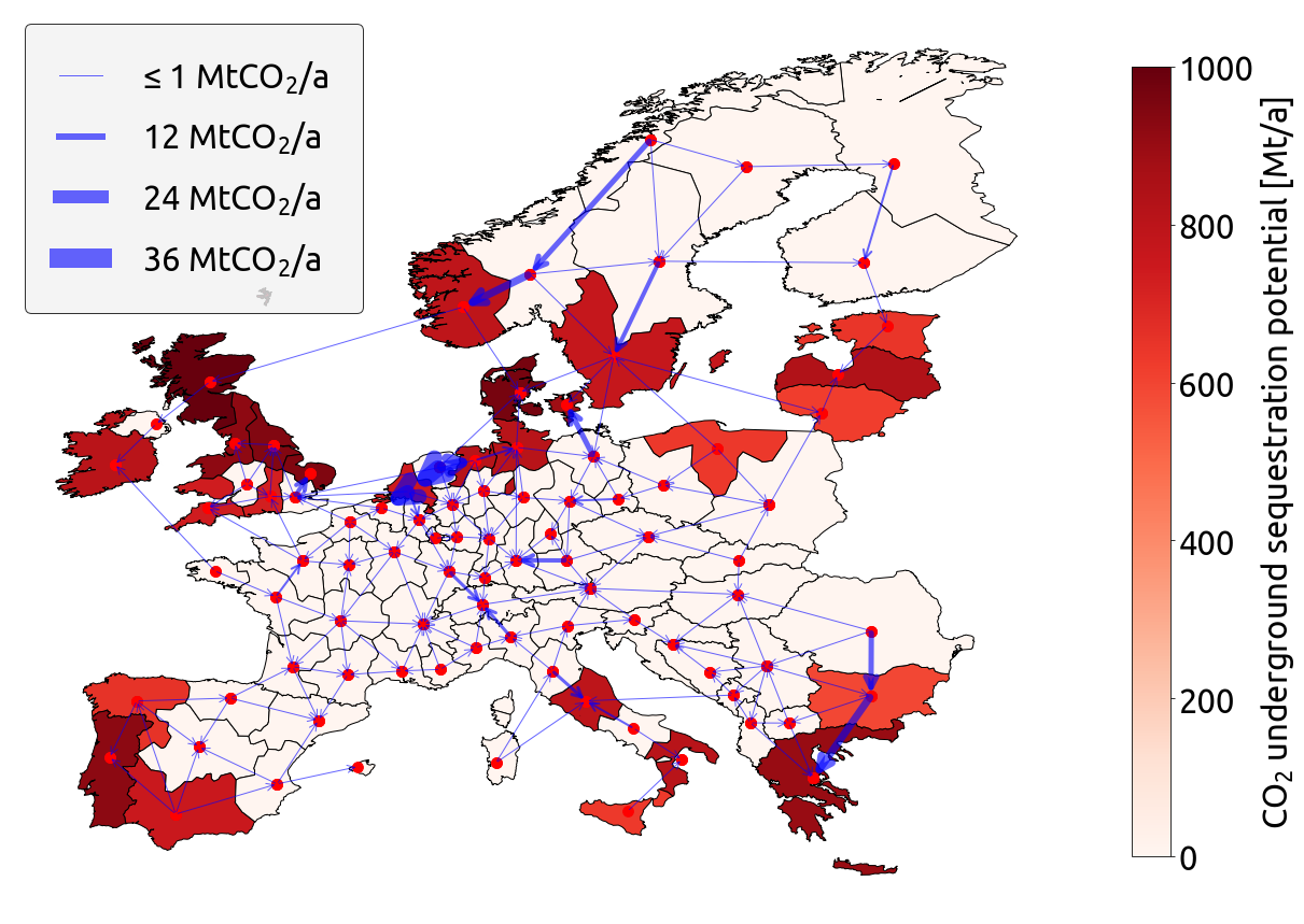
(b)

Figure 5: CO₂ flow in (a) the global net-zero CO₂ emissions scenario and (b) the local net-zero CO₂ emissions scenario. Under local constraints, the flow of CO₂ decreases by 30% on the continent relative to a global constraint. This happens because net absorber countries capture less CO₂ and consequently send less CO₂ to neighbouring countries through pipelines for underground sequestration and/or to produce additional synthetic oil and methanol.

2.5 Solid biomass transportation

Solid biomass can be transported by road across Europe, enabling countries to (indirectly) exchange CO₂ amongst and within themselves. In a global and local net-zero CO₂ emissions scenarios, 87 PWh·km/a and 92 PWh·km/a of solid biomass are transported, respectively (Figure 6). Based on the stoichiometric ratios provided in Table S5 and assuming that 50% of the solid biomass is carbon, this is equivalent to effectively moving 32 GtCO₂·km/a in a global scenario and 34 GtCO₂·km/a in a local scenario, making this method the second most relevant in distributing CO₂ across Europe.

In both scenarios, the transportation pattern for solid biomass in Europe involves countries or regions with a high demand but low potential for this material, which are supplied by neighbouring countries or regions with a higher potential. This typically occurs from eastern central to western central Europe.

Under local net-zero CO₂ emissions constraints, we observe a rise in the transportation of solid biomass from Poland and the Czech Republic to Germany, and from Sweden to Norway. This is due to the growing use of solid biomass-based CHP units with CC in the importing countries to meet their heat and power requirements (Figures 3 and S19). In addition, there are noticeable variations in solid biomass transportation within Germany. The transportation increases from its central regions to its western regions and decreases within its southern regions to meet the different solid biomass demand and potential levels in these regions. In both scenarios, large amounts of solid biomass are transported from France to Great Britain and Belgium, from Germany to the Netherlands, and from northern Finland, Latvia, and Lithuania (via Latvia) to southern Finland. While Great Britain, Belgium, and the Netherlands primarily import solid biomass due to their low potential for this material (Figure S10), southern Finland does so due to its high demand for solid biomass.

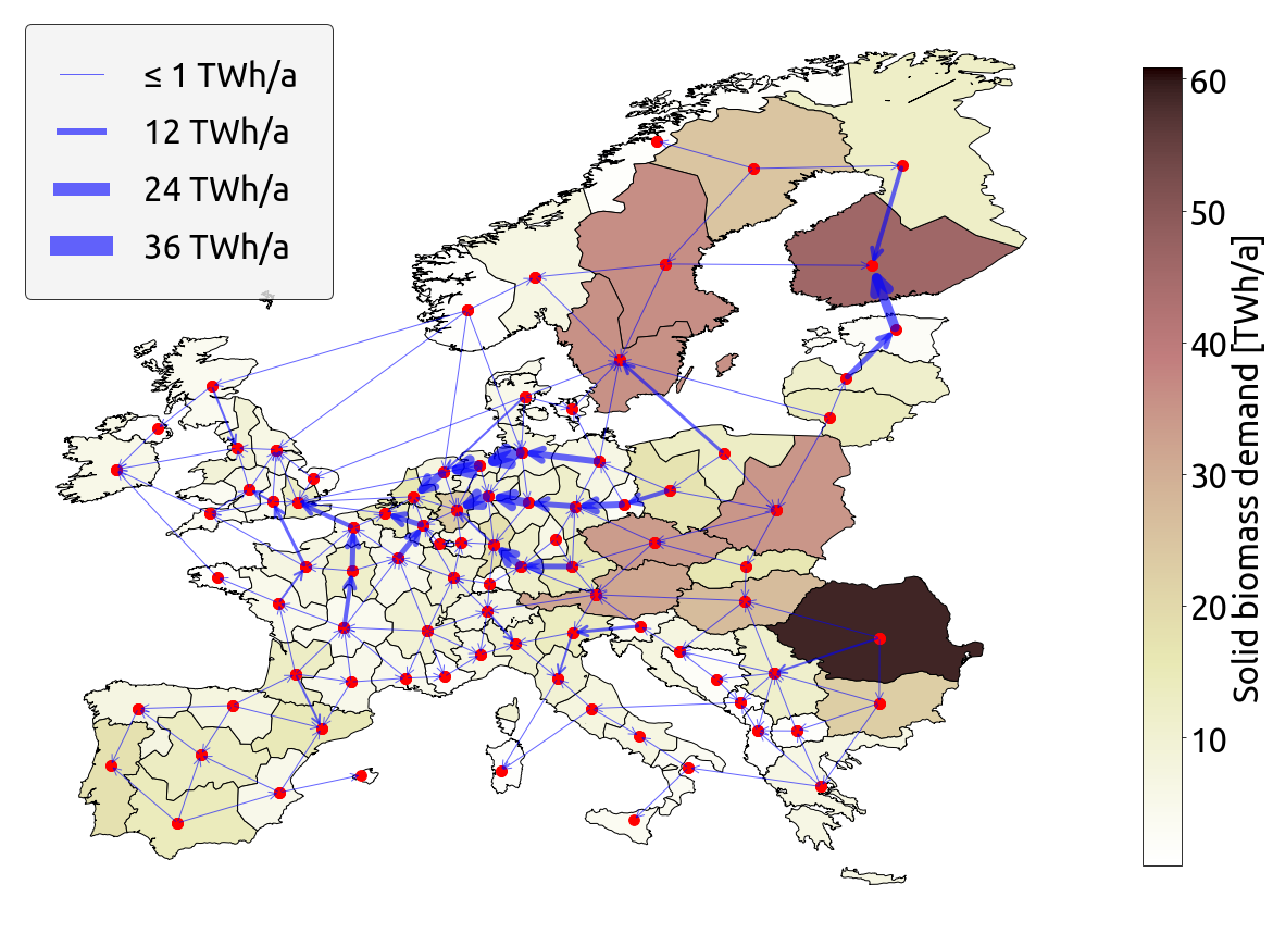
(a)

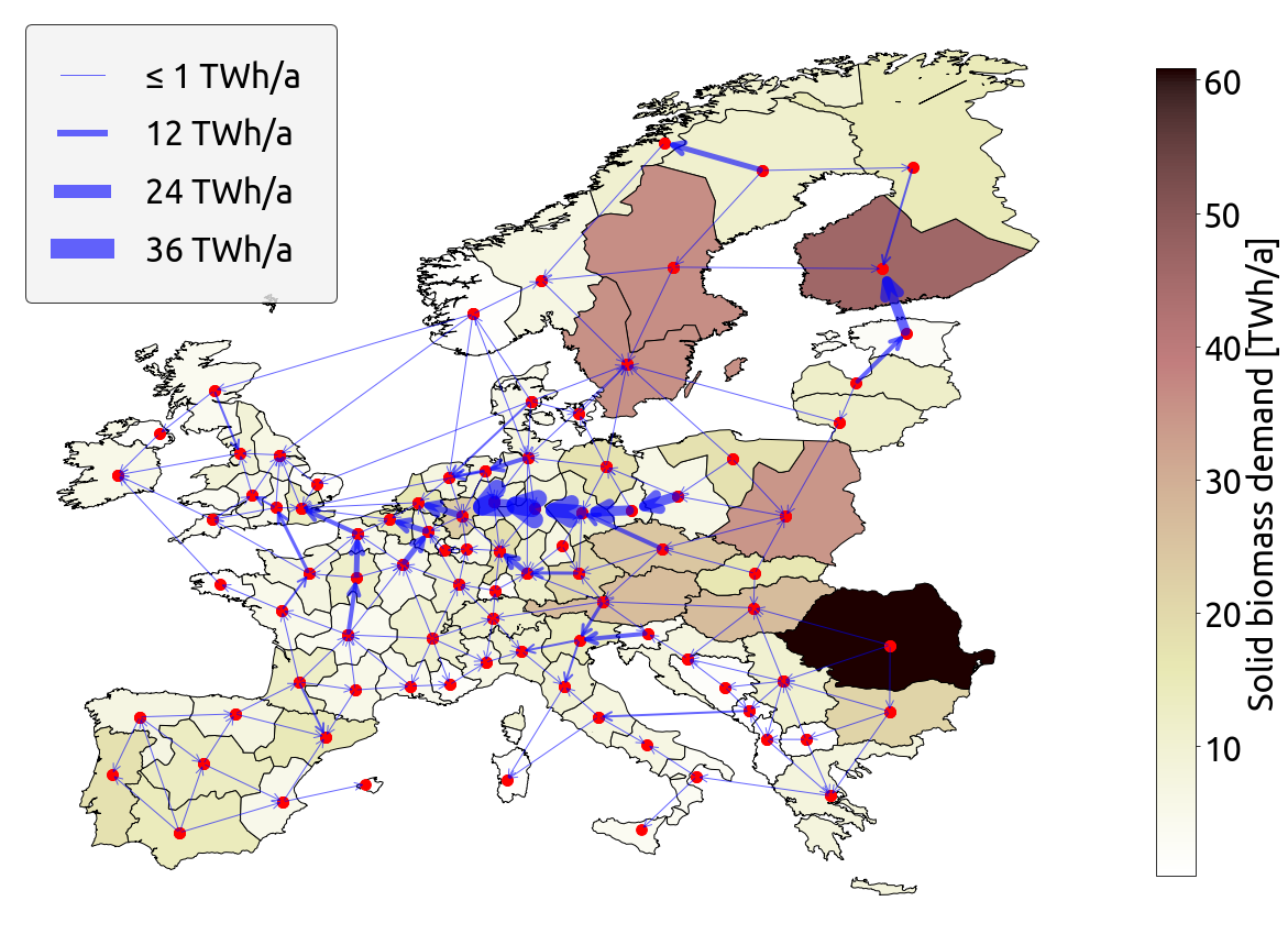
(b)

Figure 6: Solid biomass transportation in (a) the global net-zero CO₂ emissions scenario and (b) the local net-zero CO₂ emissions scenario. In both scenarios, solid biomass transportation concentrates in central Europe, moving from the East, where there is high solid biomass potential, to the West, where there is high demand for solid biomass but low local potential.

2.6 Methane gas flow

Methane gas can be transported through a network of pipelines, allowing countries to exchange this material amongst themselves and within their borders, as well as indirectly transport CO₂. In a global and local scenarios aiming for net-zero CO₂ emissions, 124 PWh·km/a and 109 PWh·km/a of methane gas are transported across the entire continent, respectively. See Figure 7.

The total methane gas consumption in Europe amounts to 800 TWh/a. This implies that, on average, 16% of that demand is transported 1000 km. Out of the annual demand, 55% of methane gas comes from synthetic or biogenic sources. Assuming the stoichiometric ratios provided in Table S5, the transportation of 124 PWh·km/a of methane gas effectively results in moving 24 GtCO₂·km/a in a global scenario, while 109 PWh·km/a of methane gas results in moving 21 GtCO₂·km/a in a local scenario. Therefore, transporting CO₂ in the form of methane gas is the third most relevant method for carbon distribution in Europe.

Important flows of methane gas driven by existing infrastructure occur in a global scenario, including the flow from the Netherlands to Germany and the flow from Greece to meet the demand in northern Italy, Switzerland, and Austria. Both flows decrease in significance in a local scenario though. The decrease in the first flow is connected to Germany requiring less methane gas, while the decrease in the second flow is due to Switzerland also requiring less methane gas and Austria being supplied by Slovakia, which starts sending a substantial amount of this material to this country (Figure S19). In addition, important flows occur within Germany and France in both scenarios to supply regions lacking methane gas. Furthermore, in a local scenario, Spain also experiences significant internal flows, originating in the south and reaching France to satisfy its demand for methane gas.

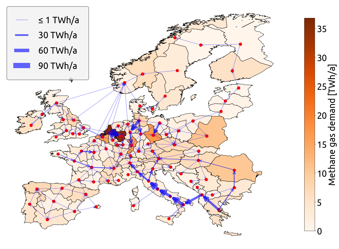
(a)

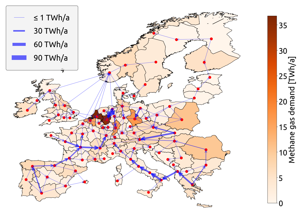
(b)

Figure 7: Methane gas flow in (a) the global net-zero CO₂ emissions scenario and (b) the local net-zero CO₂ emissions scenario. Most of the flows occur to satisfy northern Italy, Switzerland, and Austria with methane gas imported mainly from Greece (in both scenarios) and Slovakia (in the local scenario). Significant flows also occur within Germany and France.

Table 1: Energy and carbon flows in the global and local net-zero CO₂ emissions scenarios. Carbon is also transported in the form of synthetic oil and methanol (Figures S20 and S21), but our model does not include a detailed representation of the networks for these energy carriers.

Material	Energy flow [PWh·km/a]		Carbon flow [GtCO2·km/a]
	Global	Local	Global	Local
CO2	-	-	124	87
Solid biomass	87	92	32	34
Methane gas	124	109	24	21
H2	518	623	-	-
Electricity	962	978	-	-

2.7 Hydrogen flow

H₂ is crucial for producing synthetic oil, methane gas, and methanol. It is also used in fuel cells, land transportation, and in the industry. As such, it is important to understand where H₂ is produced and how it is transported across Europe, as well as how these differ between global and local climate-neutral scenarios.

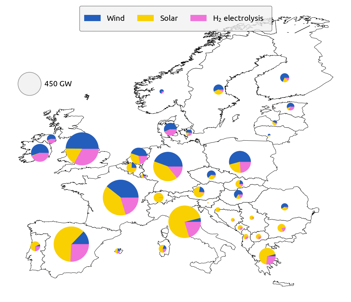
(a)

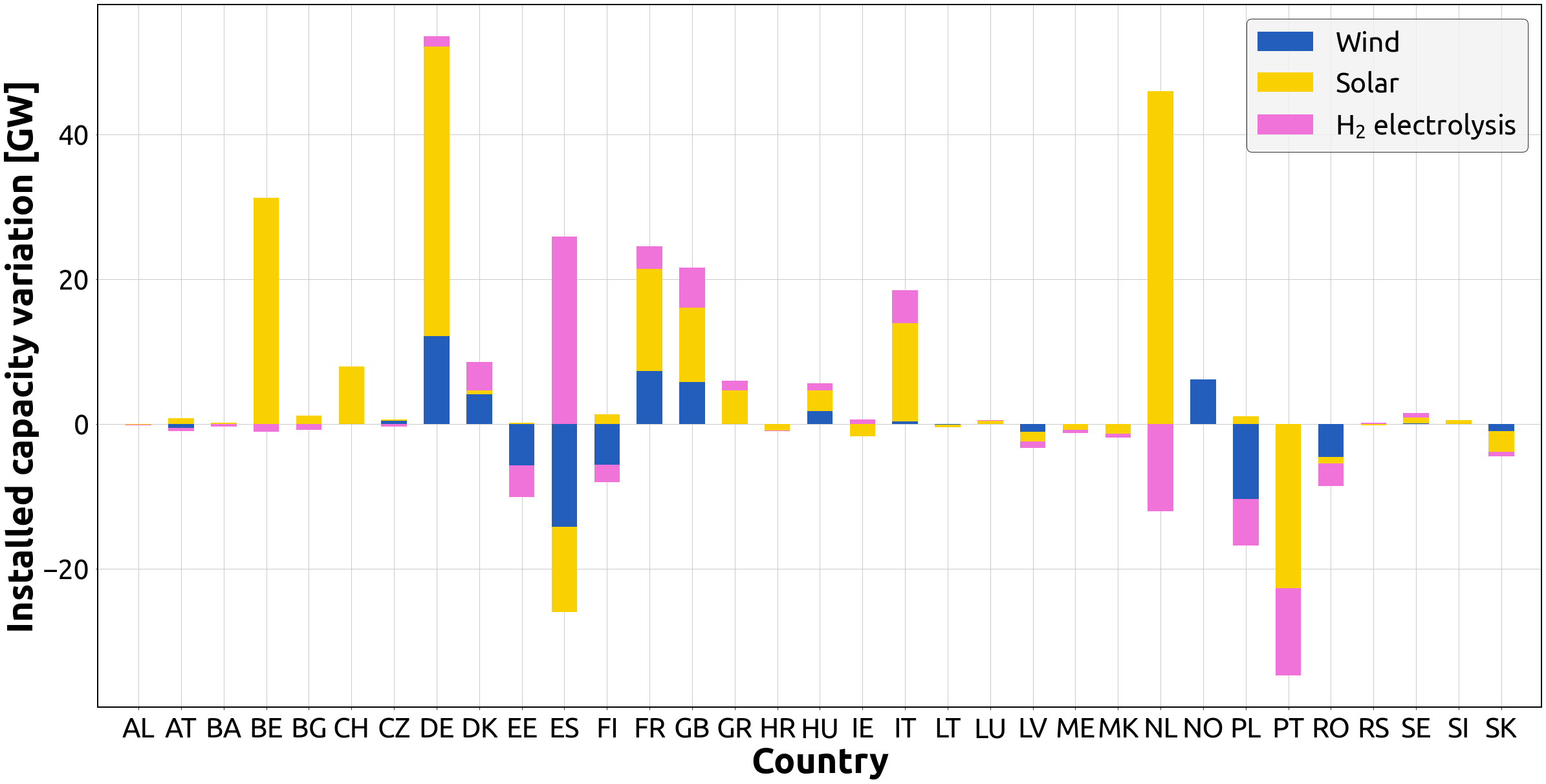
(b)

Figure S28: (a) Wind, solar, and H₂ electrolysis installed capacity in the global net-zero CO₂ emissions scenario and (b) Wind, solar, and H₂ electrolysis installed capacity variation per country between the global net-zero CO₂ emissions scenario and the local net-zero CO₂ emissions scenario.

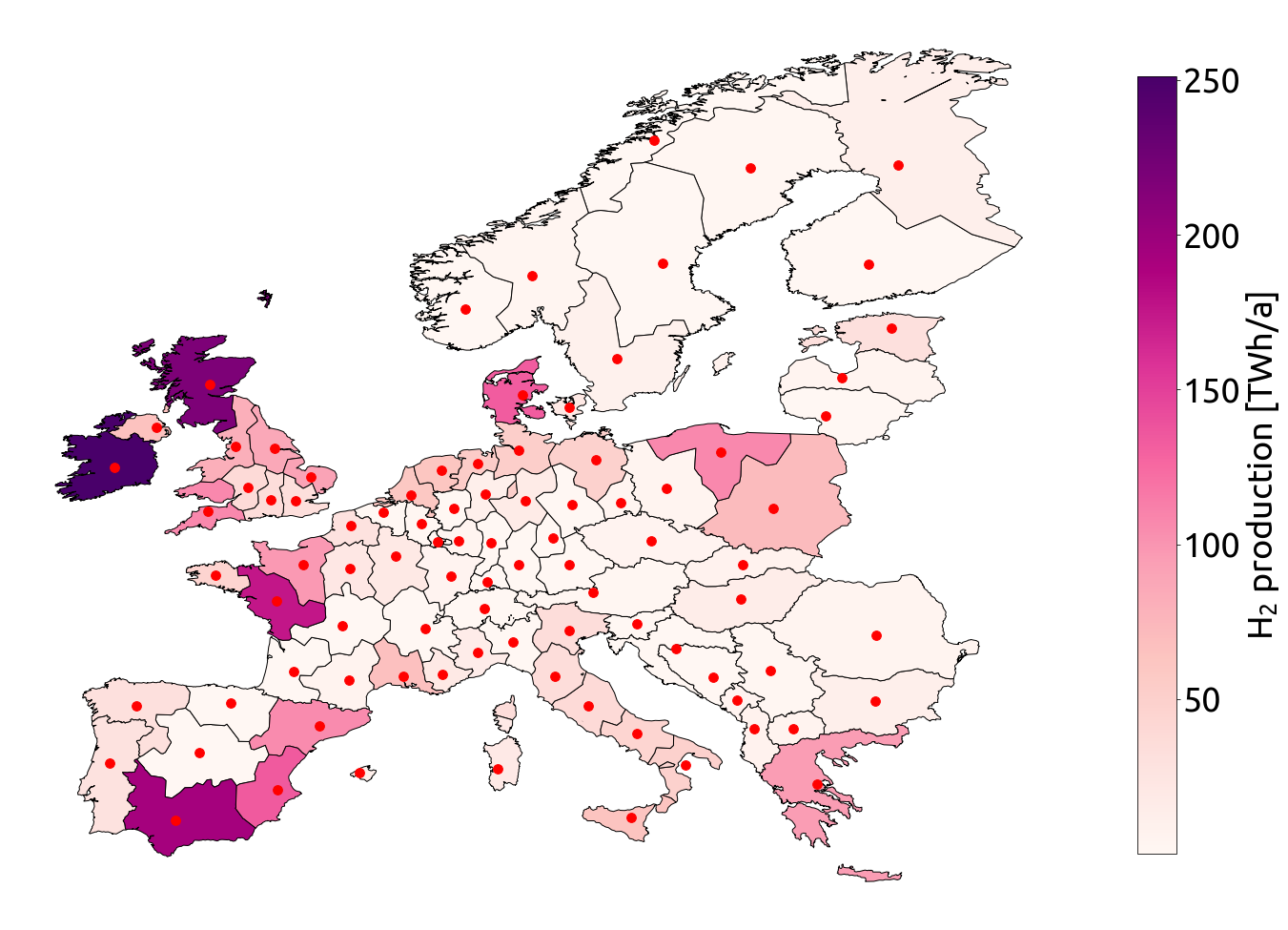
(a)

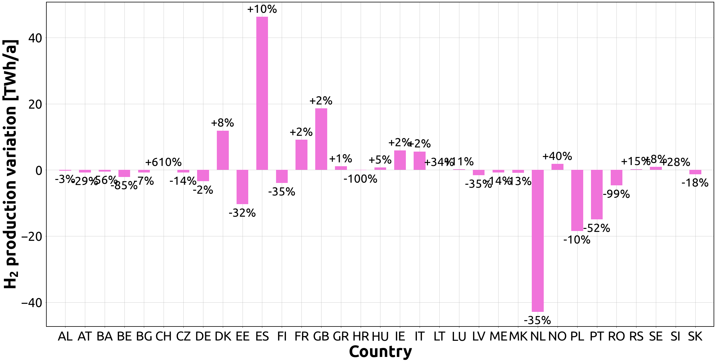
(b)

Figure S29: (a) H₂ production in the global net-zero CO₂ emissions scenario and (b) H₂ production variation between the global net-zero CO₂ emissions scenario and the local net-zero CO₂ emissions scenario. Thanks to high renewable energy capacity factors and their relative proximity to the interior countries and Switzerland, Spain, Denmark, and Great Britain significantly increase H₂ production to satisfy a growing demand for H₂ in the former countries when under local constraints.

In both scenarios, the flow of H₂ is driven by the demand for this material and the cost-effective locations in Europe with high wind and solar resources (Figure S9). From this perspective, the main countries that produce electrolytic H₂ in Europe are Great Britain, France, Spain, Italy, and Ireland (Figure S28). These locations were also identified in [12]. Despite being the largest H₂ producers in a global scenario, they further increase production levels in a local scenario. Conversely, the interior countries decrease their H₂ production levels (Figures S29 and S30).

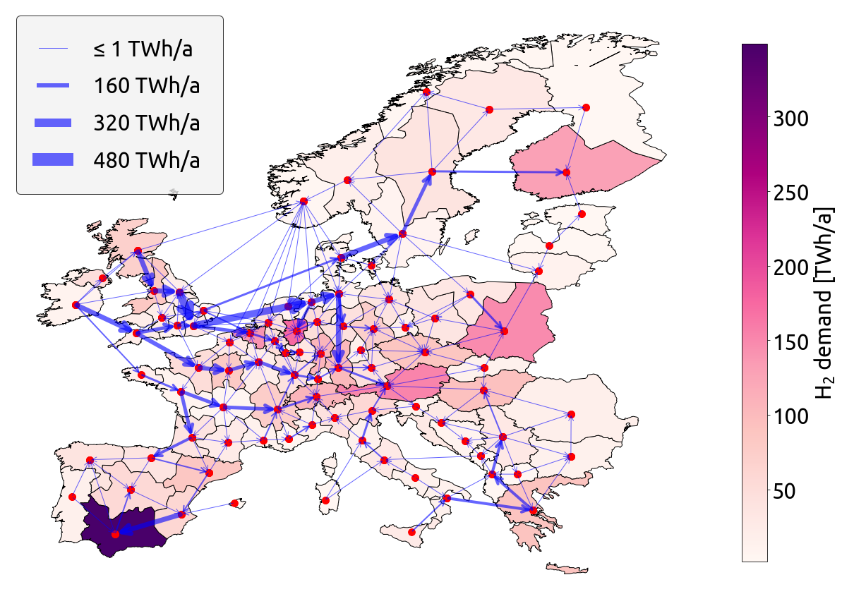
(a)

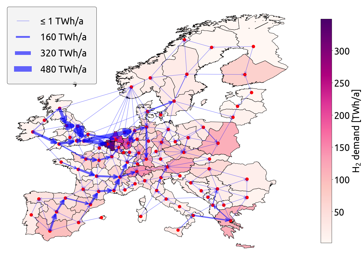
(b)

Figure S26: H₂ flow in (a) the global net-zero CO₂ emissions scenario and (b) the local net-zero CO₂ emissions scenario. The total amount of H₂ flowing amongst and within countries increases by 6% under local constraints relative to the global constraint. Most of this increase is to provide the necessary H₂ for the interior countries and Switzerland to meet their industrial needs and produce more synthetic oil and methanol under the local scenario.

Under local constraints, we observe a 20% (105 PWh·km/a) increase in the flow of H₂ compared to the 518 PWh·km/a flowing under a global constraint (Figure S26). This increase can be explained as a side effect of the reduction in CO₂ flows. As discussed in [11], when the carbon flows are lower (in the local scenario), H₂ produced in locations with high renewable resources need to be transported to where the carbon is collected to be combined and produce synthetic fuels.

2.8 Electricity flow

Electricity is required in large quantities to enable direct-air-captured CO₂ and methanalisation to transform captured CO₂ into methanol. It is also vastly needed for producing H₂ electrolytically, a key component in manufacturing synthetic products. This emphasises the importance of understanding where electricity is produced and transmitted amongst and within countries for consumption.

In a climate-neutral scenario, the production of electricity in Europe is mainly determined by the accessibility of cost-effective renewable energy. Furthermore, although nuclear power plants are an option for producing electricity in our model, they are not chosen because of their high cost. From this perspective, major production is observed in Great Britain, France, Spain, Germany, and Italy. In a global scenario, a total of 10068 TWh of electricity is produced annually, with a slight increase of 1.1% in a local scenario (Figures S28 and S16). The model’s intrinsic constraint for the electricity supply to meet the demand on an hourly basis provides stability for the entire system (Equation S2), resulting in minimal production differences when comparing the two scenarios.

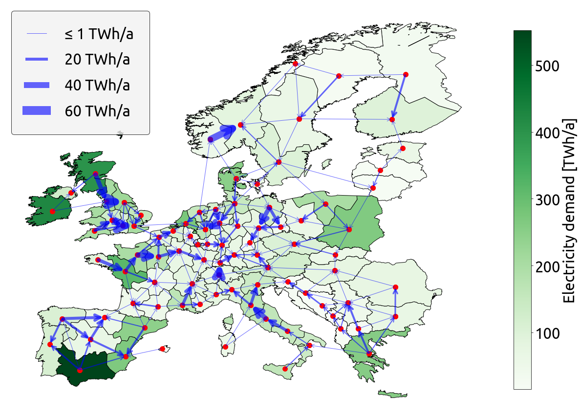
(a)

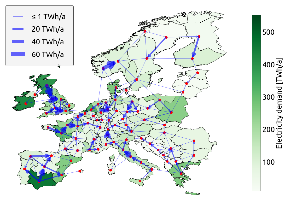
(b)

Figure S27: Electricity flow in (a) the global net-zero CO₂ emissions scenario and (b) the local net-zero CO₂ emissions scenario. In both scenarios, most of the electricity flows are confined within individual countries. Regions within the same country supply electricity to each other to power DAC and methanolisation, as well as H₂ production, with limited electricity exchange occurring between countries.

For simplicity, we do not allow expansion of transmission capacity beyond today’s values. This results in a flow of electricity that amounts to 962 PWh·km/a in a global scenario and 978 PWh·km/a in a local scenario (Figure S27). In both scenarios, most of the electricity flows within each country, typically those that produce the most H₂ in Europe (Figures S29).

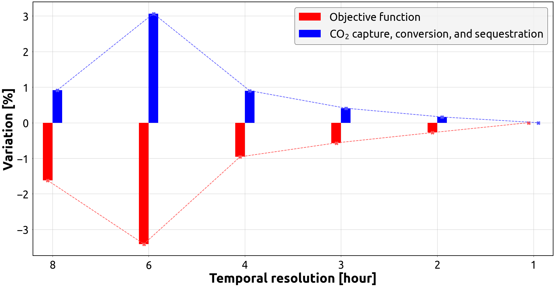
(a)

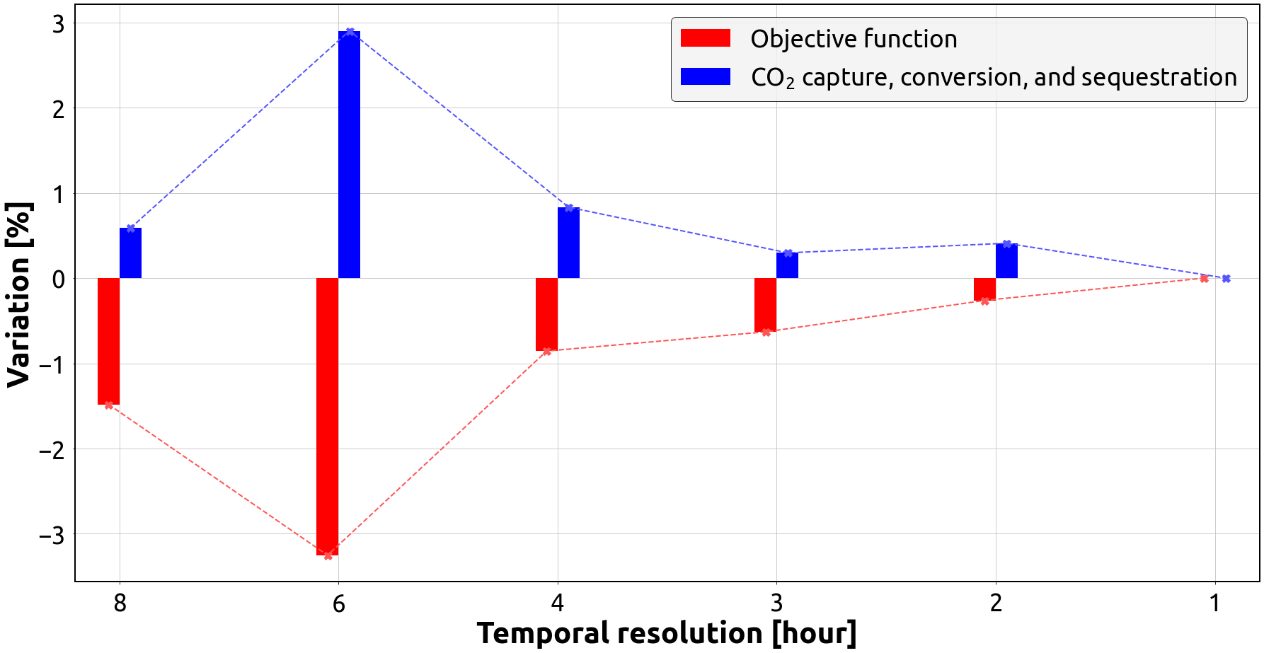
(b)

Figure S5: Sensitivity analysis of the model under different temporal resolutions in (a) the global net-zero CO₂ emissions scenario and (b) the local net-zero CO₂ emissions scenario. Due to computational limitations, both sensitivity analyses were conducted with an 80-node spatial resolution of the model instead of the 90-node spatial resolution used in our study. The red and blue bars show the variations of the objective function and the aggregated amount of CO₂ captured, converted, and sequestered underground, respectively, in comparison to the baseline of one-hour temporal resolution.

In this paragraph, we briefly discuss the limitations of our analysis. First, the model presented in this study is based on an overnight greenfield optimisation and assumes perfect foresight. This might have missed some of the technological lock-ins or path-dependent effects during the system transformation. Exogenous cost assumptions summarised in Table LABEL:supplemental:table_technology_characteristics_assumptions might be different which could affect the results. As described in the Methods section, only the most relevant technologies for capturing CO₂ are included in the model. The temporal resolution of the model is 3 hours, which is sufficient for our study compared to the highest temporal resolution of 1 hour allowed in PyPSA-Eur (see Figure S5). The model assumes that Europe produces all synthetic fuels it needs and does not rely on imports from other regions.

3 Conclusions

In this study, we modelled the European sector-coupled energy system, imposing a net-zero CO₂ emissions target in each country. We then compared the results from this model with those of a global net-zero CO₂ emissions target imposed on the entire continent and analysed the implications of this on the system from various perspectives.

Regarding emissions, we showed that, in a global scenario, countries can either be net CO₂ emitters or absorbers. The first release more CO₂ than they capture, while the second capture more CO₂ than they release on a yearly average. Under this light, Germany, Belgium, and the Netherlands are the biggest net CO₂ emitters. Spain, Sweden, Finland, Poland, and Romania, on the other hand, are the most prominent net CO₂ absorbers.

From an economic standpoint, our results revealed that a system in a local scenario leads to a rise of 1.4% in total cost. This means that, with a slight additional cost, Europe can attain a more equitable climate-neutral energy system costing 890 billion € per year. Furthermore, to achieve a fully decarbonised continent, a price of 540 € per tonne of CO₂ is necessary in a global scenario. However, the price needed to achieve the same goal varies significantly amongst countries in a local scenario, ranging from 402 € in Latvia to 584 € in Belgium per tonne of CO₂, due to their disparate CO₂ emissions sources and volumes, as well as renewable resources.

From an operational perspective, we demonstrated that countries that are net emitters under a global constraint capture much more CO₂ mainly through DAC under local constraints to achieve climate neutrality on their own, as they can no longer rely on other nations with low-cost energy to counterbalance their emissions. Conversely, net absorber countries reduce CO₂ capture from DAC, as well as from point sources. When it comes to CO₂ conversion, net emitter countries produce more synthetic oil and methanol in a locally constrained scenario. This is a result of these countries capturing additional CO₂, which must be dealt with. In contrast, net absorber countries reduce synthetic products manufacturing due to capturing less CO₂ in this scenario. Sequestering CO₂ underground is considered the most cost-effective option by the model to handle captured CO₂, depleting the assumed conservative potential of 200 MtCO₂/a in both scenarios.

We found that the three methods of transporting captured CO₂ in our model are important to balance the demand and supply of this material amongst countries in both scenarios. A purposely built CO₂ network is the most prominent in this task, followed by the exchange of CO₂ through solid biomass and methane gas. Despite its importance, achieving a climate-neutral energy system without a CO₂ network would only result in a minimal cost increase in both scenarios.

Overall, this study highlighted the importance of better understanding the capture, transportation, conversion, and sequestration of CO₂ under national emissions targets, as this better reflects Europe’s efforts to decarbonise. Doing so provides a clearer picture for organisations to develop the most critical technologies to support these efforts. This also makes it more relevant for each nation, helping to determine the necessary installation capacity of the selected technologies and establish appropriate regulations according to their specific needs.

To address some limitations of this study, we plan to improve the model by adopting a myopic approach (which better matches policymakers’ decision-making process) and focus on the heaviest net CO₂ emitter and absorber countries (as they influence the most the energy system under net-zero CO₂ emissions targets) in a future study. This will advance our understanding of how Europe can attain climate neutrality by 2050 by identifying potential transition pathways in a realistic manner.

4 Methods

4.1 Model

The present study relies on PyPSA-Eur[13], an open-source model based on PyPSA [14] that is used to optimise the capacity and dispatch of an energy system covering the entire European Network of Transmission System Operators for Electricity (ENTSO-E) area. This encompasses 33 European countries: the EU27 (excluding Malta and Cyprus), Norway, Switzerland, Great Britain, Albania, Bosnia and Herzegovina, Montenegro, Macedonia, and Serbia. PyPSA-Eur comprises the electricity, heating, land transport, shipping, aviation, and industry sectors, including industrial feedstocks. It represents generators, stores, transmission lines, and converting technologies in different sectors of an interconnected energy system and provides a detailed account of CO₂ capture, usage, and storage (CCUS). PyPSA-Eur assumes long-term market equilibrium, perfect competition and foresight.

At its core, the model uses linear programming to determine the most cost-effective energy system based on a set of constraints, with the most important constraints for this study being the allowable limit for CO₂ emissions (Equations S3 and S4). Refer to Supplemental 1 for a mathematical formulation of the linear programme.

The characteristics of the technologies, including costs, efficiencies, and lifetimes, are based on data from the Danish Energy Agency [15] and are summarised in Table LABEL:supplemental:table_technology_characteristics_assumptions. Characteristics assumptions for the year 2030 [16] are chosen for the model because they are less uncertain than those for a more distant year, such as 2050.

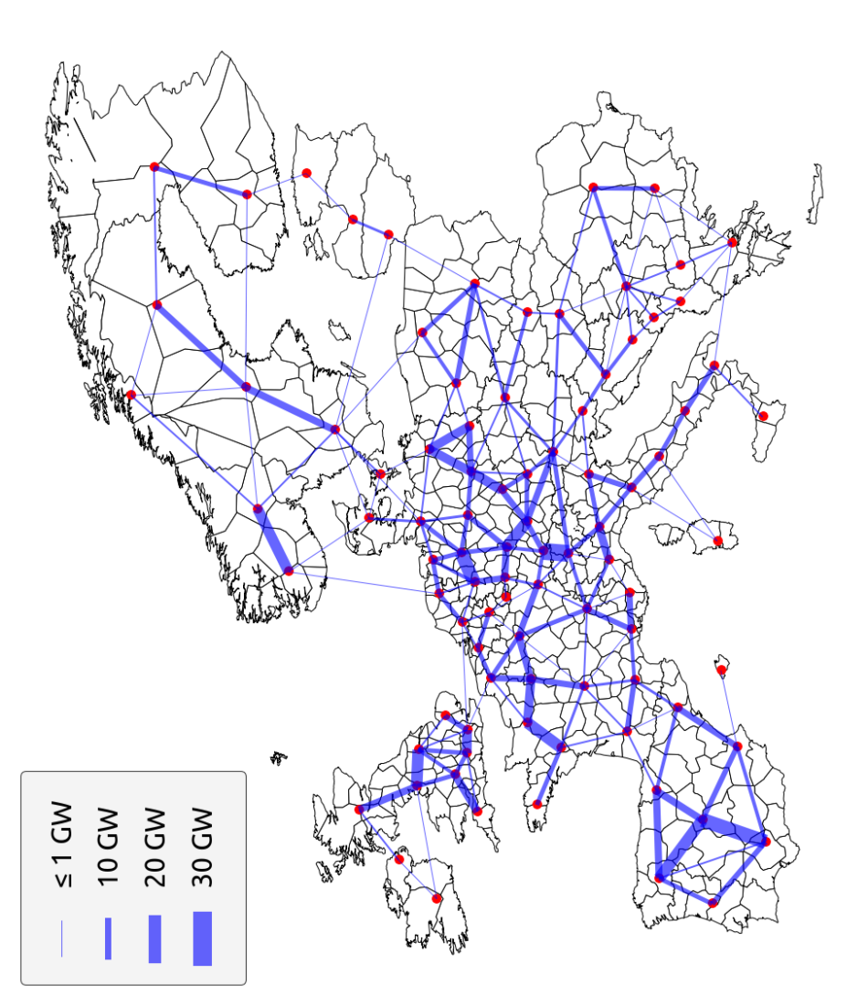
Figure S1: The European energy system spatial layout spanning across 33 countries in both the global and local net-zero CO₂ emissions scenarios. It is modelled with a 90 nodes resolution (indicated by red dots) and 370 regions representing renewable resources, with each region associated with one of the nodes. The (blue) lines connecting nodes represent the electricity grid topology, which includes both existing power lines and new ones planned for construction in Europe as per ENTSO-E’s TYNDP 2018.

The model is set up to represent the European energy system characterised by net-zero CO₂ emissions, either globally imposed for the whole of Europe or locally for each of the 33 European countries. It performs an overnight greenfield optimisation of the energy network system, which consists of 90 nodes, 370 regions representing renewable resources (each associated with one of the nodes), and a 3-hour time resolution for the entire year. See Figures S1 and S5. This setup represents well the European landscape and the variations in wind and solar patterns throughout the day, week, and season [17]. It also addresses the concerns raised in [18] and [19] regarding sufficient spatial and temporal resolution, while still being computationally feasible [20] [21]. The renewable energy capacity factors in Europe were calculated using atlite [22] and data from a single year of weather provided by ERA5 [23]. Here, 2013 was chosen as it represents a year with average wind and solar resources [24, 25].

The transmission capacity of the electricity grid is exogenously fixed (i.e. the model is not allowed to increase its capacity) and it includes existing lines as well as new ones to be built in Europe, in accordance with ENTSO-E’s Ten-Year Network Development Plan 2018 [26] (Figure S1).

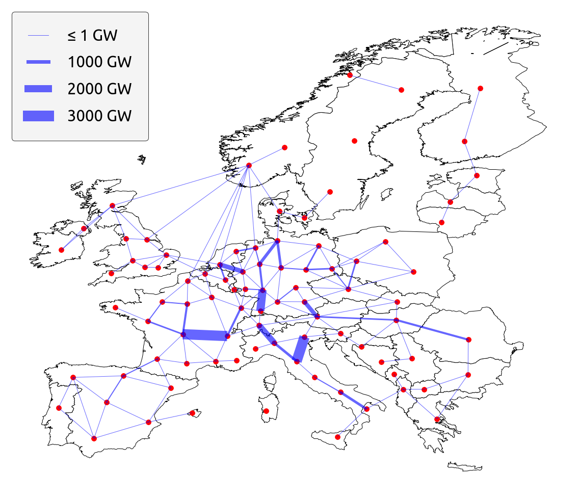
(a)

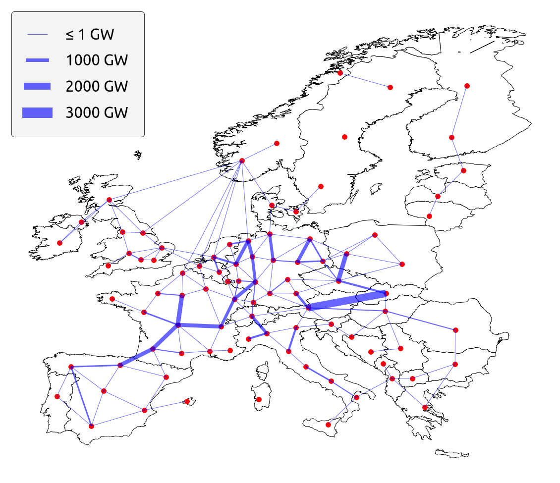
(b)

Figure S2: The European methane gas network topology in (a) the global net-zero CO₂ emissions scenario and (b) the local net-zero CO₂ emissions scenario. Each pipeline has a specific capacity and is organised according to the SciGRID_gas project, which forms the basis for transporting methane gas in the model. The model is allowed to expand the capacity of pipelines if it reduces the total system cost.

The model allows the transportation of methane gas through pipelines (Figure S2), which are organised and have limited capacities according to the SciGRID_gas [27] project. This project represents the existing methane gas network currently installed in Europe. The model is allowed to expand pipelines’ capacities if it reduces the total system cost. Furthermore, due to compression losses, these have a transportation efficiency of 99% per 1000 km.

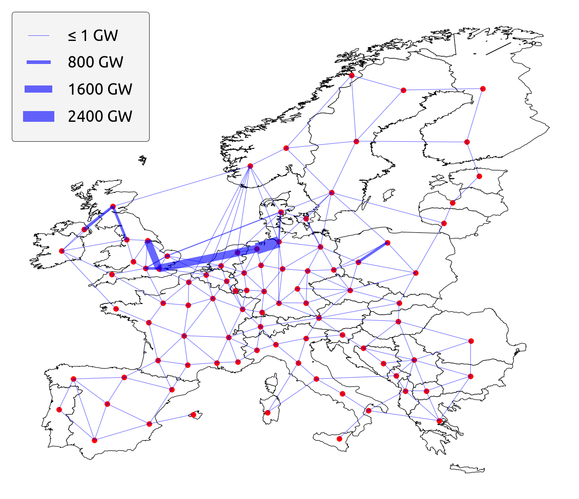
(b)

Figure S3: The European H₂ network topology in (a) the global net-zero CO₂ emissions scenario and (b) the local net-zero CO₂ emissions scenario. The model is allowed to build new H₂ pipelines if it reduces the total system cost. These have optimal capacities and are organised according to the electricity grid and methane gas network topologies.

The model is allowed to build bidirectional pipelines to transport hydrogen (H₂) with optimal capacities also when deemed cost-effective. Due to compression losses, pipelines have a transportation efficiency of 98.2% per 1000 km. For simplicity, these are spatially arranged based on the existing electricity grid and methane gas network topologies (see Figure S3).

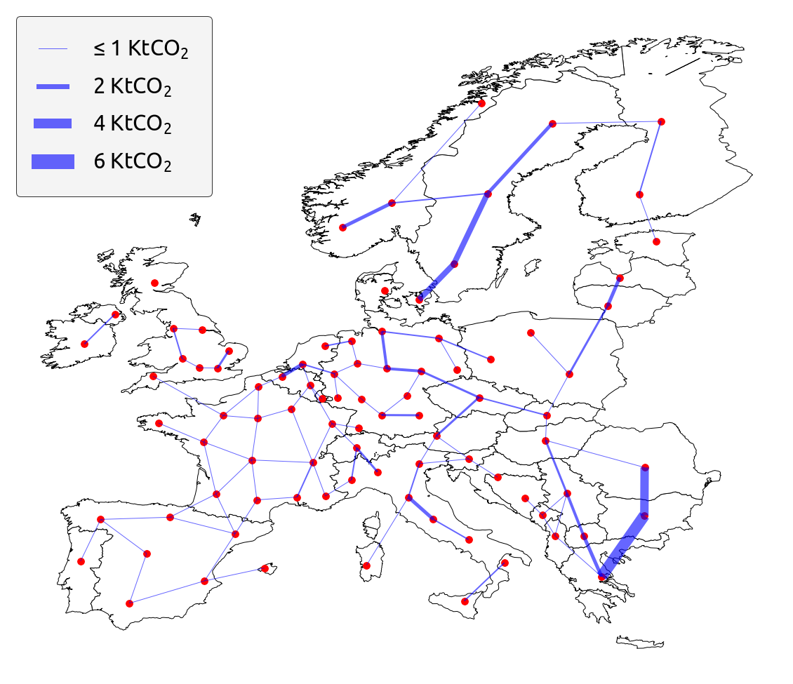
(a)

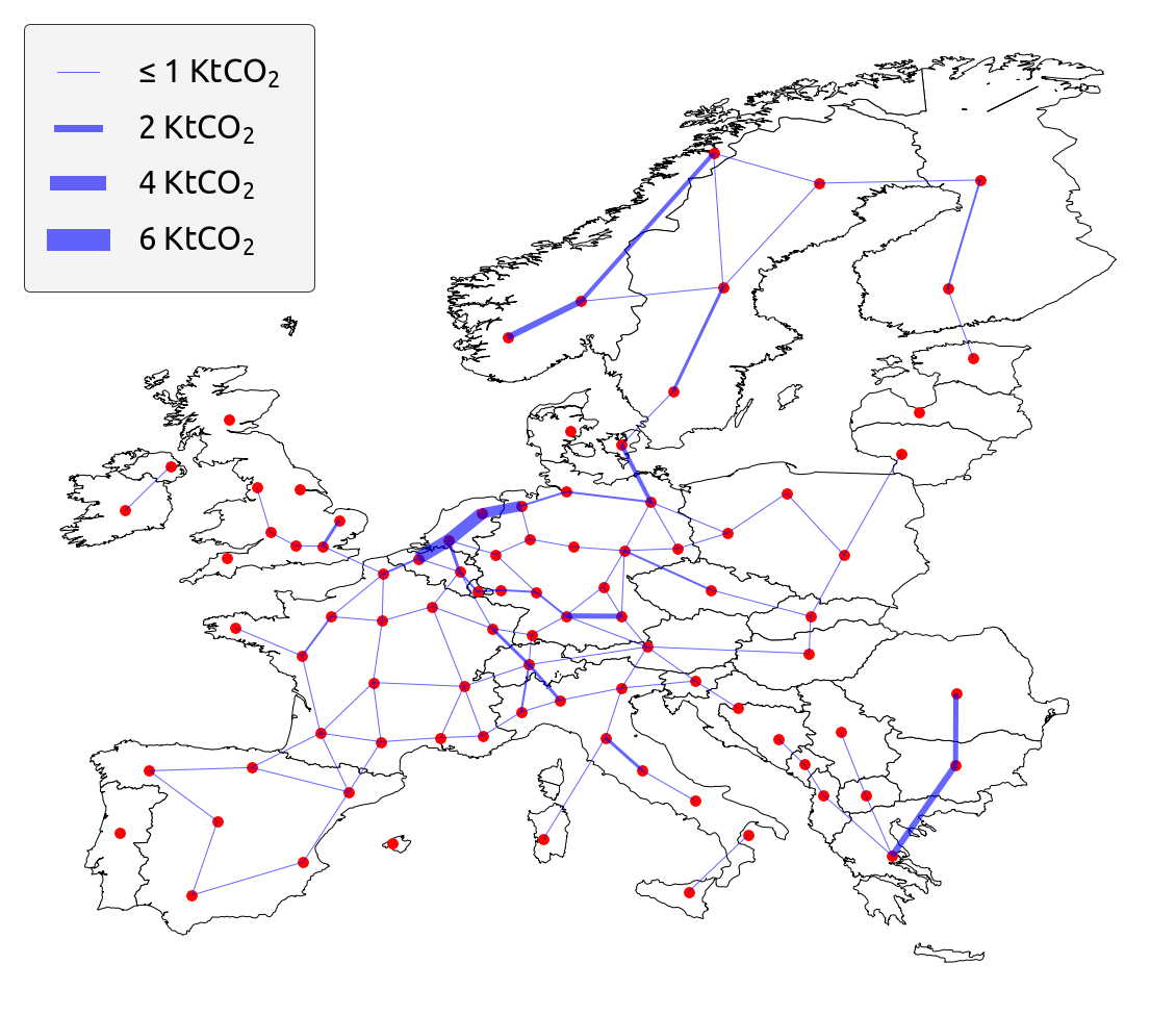
(b)

Figure S4: The European CO₂ network topology in (a) the global net-zero CO₂ emissions scenario and (b) the local net-zero CO₂ emissions scenario. The model is allowed to build new CO₂ pipelines if it reduces the total system cost. These have optimal capacities and are organised according to the electricity grid topology.

CO₂ can be transported through a network of pipelines (see Figure S4). The model is allowed to build bidirectional, lossless pipelines when deemed cost-effective with optimal capacities. For simplicity, these are spatially arranged based on the existing electricity grid topology.

In addition, the model allows the transportation of solid biomass amongst countries representing the potential transport by road. The cost of transportation for each country is based on the JRC-EU-TIMES model (Table S2).

Oil and methanol, on the other hand, have unlimited transportation capacity amongst countries in the model. The possibility of importing and exporting synthetic fuels to and from Europe is not modelled.

The capacities of run-of-river (ROR), hydroelectricity, and pump hydro storage (PHS) are exogenously set in the model based on existing facilities in Europe.

The model only includes CO₂ emissions from energy consumption in the agriculture sector, and it assumes that the rest of CO₂ emissions from this sector are offset by the Land Use, Land Use Change, and Forestry (LULUCF) sector.

4.2 Carbon capture

In our model, CO₂ can be captured from process emissions in industries, gas and solid biomass used in industry, CHP units combusting methane gas or solid biomass, steam methane reforming (SMR) to produce H₂, and biomass used to produce biogas, which is then upgraded to methane gas. For the latter, a 90% capture rate is assumed. In addition, CO₂ can be captured using DAC, which is modelled as a low-temperature heat-requiring system. DAC can be installed collocated with industrial demands where the required heat is supplied by air heat pumps, methane gas boilers, and resistive heaters. It can also be installed connected to district-heating system in urban areas. In this case, apart from the mentioned sources, the required heat is supplied by solar thermal, gas and solid biomass-based CHP units, along with the excess heat from the Fischer-Tropsch process and H₂ fuel cells.

Additional methods for capturing CO₂, such as bioenergy with carbon capture and storage (BECCS), enhanced rock weathering, biochar, agroforestry, afforestation/reforestation, soil carbon sequestration, coastal wetland management, ocean alkalinisation, and ocean fertilisation and artificial upwelling [28], have been excluded from the model. While BECCS is not considered, our model does account for conservative amounts of biomass, i.e., biomass not competing with food crops. First, solid biomass includes agricultural waste, fuelwood residues, secondary forestry residues (woodchips), sawdust, residues from landscape care, and municipal waste. A potential of 1038 TWh per year of solid biomass is assumed for Europe, based on the medium bioenergy availability scenario of the ENSPRESO database [29]. This solid biomass can be used to produce heat in the industry or combusted in CHP units, in both cases with or without carbon capture (CC). Biomass import from outside the continent is not allowed. The model also includes biogas, with a potential of 336 TWh/a for Europe, which is upgraded to methane gas. Furthermore, although promising results have been recently shown for direct ocean capture (DOC) of CO₂ [30], we do not model this technology.

The amount of process emissions and gas and solid biomass demand in the industry are exogenous to the model, while CHP and DAC capacities are endogenous.

4.3 Carbon conversion and sequestration

In the model, CO₂ can be converted (used) to manufacture valuable products such as synthetic oil through the Fischer-Tropsch process, synthetic methanol through methanolisation, and synthetic methane gas through the Sabatier reaction. While synthetic oil and methane gas production are endogenous to the model, the production of methanol is exogenous to the model since its demand is exogenously set.

In addition, CO₂ can be sequestered underground in the model. Despite Europe having a huge potential for sequestering CO₂ both onshore and offshore, estimated at 117 Gt [31], the model restricts this to 2.1 Gt and only considers offshore underground potential, specifically in deep saline aquifers and depleted hydrocarbon reservoirs. Table S3 summarises how this amount is shared amongst countries. Based on these shares, the model optimally determines the amount of CO₂ that can potentially be sequestered in each country. Furthermore, since CO₂ sequestration is a highly uncertain technology, the model is constrained to a maximum annual sequestration of 200 MtCO₂ for the entire continent. This amount allows for sequestering process emissions, which, assuming an industrial transformation, account for 153 MtCO₂ per year in Europe, with the remaining 47 MtCO₂ enabling negative emissions. A lower amount would make the model unfeasible under a net-zero CO₂ emissions constraint. A sensitivity analysis to the assumptions for potential and cost for CO₂ underground sequestration can be found in [9] and in Figure S25.

5 Experimental procedures

5.1 Lead contact

Further information and requests for resources should be directed to and will be fulfilled by the lead contact, Ricardo Fernandes (ricardo.fernandes@mpe.au.dk).

5.2 Materials availability

This study did not generate new unique materials.

5.3 Data and code availability

The model used in this study is based on a fork of PyPSA-Eur version 0.8.0, which includes new logic that implements local (national) CO₂ constraints. The fork is available at https://github.com/ricnogfer/pypsa-eur.

The technology assumptions in the model are based on the Energy System Technology Data version 0.5.0 for the year 2030 and are available at https://github.com/PyPSA/technology-data.

The energy system networks that this study is based on have been deposited in Zenodo and are available at https://doi.org/10.5281/zenodo.12527792.

6 Acknowledgments

R.F. is fully funded by Novo Nordisk CO₂ Research Center (CORC) under grant number CORC005. We sincerely thank Sleiman Farah, Alberto Alamia, and Ebbe Kyhl Gøtske, all from the Energy System Modelling Group at Aarhus University, for their scientific insights and technical support.

7 Author contributions

Conceptualisation, R.F. and M.V.; Software, R.F. and M.V.; Investigation, R.F.; Project Administration, R.F. and M.V.; Visualisation, R.F.; Resources, R.F. and M.V.; Writing-Original Draft, R.F. and M.V.; Writing-Review & Editing, R.F. and M.V.; Supervision, M.V. and M.G.

8 Declaration of interests

The authors declare no competing interests.

Supplemental 1 Mathematical formulation of the model

The model used in our study is based on PyPSA-Eur, which relies on a linear programme to minimise the total annualised cost of the entire energy system in an optimal fashion. Formally, this minimisation is represented by the following objective function:

$$\min_{G_{n,s},E_{n,s},F_{l},g_{n,s,t}}\left[\sum_{n,s}c_{n,s}G_{n,s}+\sum_{n,s}\hat{c}_{n,s}E_{n,s}+\sum_{l}c_{l}F_{l}+\sum_{n,s,t}o_{n,s,t}g_{n,s,t}\right]$$ (S1)

where, for technology $s$ in node $n$, $c_{n,s}$ is the annualised cost for generator power capacity $G_{n,s}$, $\hat{c}_{n,s}$ is the annualised cost for storage energy capacity $E_{n,s}$, $c_{l}$ is the fixed annualised cost for capacity $F_{l}$ of link $l$, and $o_{n,s,t}$ are the marginal costs of generation and storage dispatch $g_{n,s,t}$ at time step $t$. In addition, the linear programme consists of several constraints. The most relevant constraints imposed on our model are succinctly described next.

At every hour, the demand for electricity must be met by the supply, which can be expressed as follows:

$$\sum_{s}g_{n,s,t}+\sum_{l}\alpha_{n,l,t}f_{l,t}=d_{n,t}\hskip 4.26773pt\leftrightarrow\hskip 4.26773pt\lambda_{n,t}\hskip 14.22636pt\forall n,t$$ (S2)

where the sum of generation and storage dispatch $g_{n,s,t}$ of technology $s$, added to the sum of power flow $f_{l,t}$ in link $l$ with a direction and efficiency $\alpha_{n,l,t}$, equals demand $d_{n,t}$ in every node $n$ at every time step $t$. The dual value $\lambda_{n,t}$ of this constraint represents the electricity shadow price for node $n$ at time step $t$.

By default, a model based on PyPSA-Eur is constrained with a global cap (limit) on CO₂ emissions. To pursue our study, we extended PyPSA-Eur with new logic to allow for two additional types of constraints on CO₂ emissions: local (national) and nodal. In detail, the global constraint applies at a continental level (Europe), requiring that all the nodes of the model comply with a specific cap on CO₂ emissions collectively. The local (national) constraint applies at a country level, requiring that (only) the nodes of a given country comply with a specific cap on CO₂ emissions assigned to the country collectively, whereas the nodal constraint applies to each node, requiring each one to comply with a specific cap on CO₂ emissions assigned to it individually. The constraint representing a model based on a global CO₂ emissions cap can be formulated as follows:

$$\sum_{n,s,t}\varepsilon_{s}\frac{g_{n,s,t}}{\eta_{s}}\leq CAP_{CO_{2}}\hskip 4.26773pt\leftrightarrow\hskip 4.26773pt\mu_{CO_{2}}$$ (S3)

where the sum of CO₂ emissions $\varepsilon_{s}$ in tonnes per each MWh${}_{\text{th}}$ produced by technology $s$ with efficiency $\eta_{s}$ in all nodes $n$ of the model must be equal to or lower than CO₂ limit $CAP_{CO_{2}}$. The dual value $\mu_{CO_{2}}$ of this constraint represents the CO₂ shadow price for the entire Europe.

The constraint representing a model based on local (national) CO₂ emissions caps can be formulated as follows:

$$\sum_{n,s,t}\varepsilon_{s}\frac{g_{n,s,t}}{\eta_{s}}\leq CAP_{CO_{2},k}\hskip 4.26773pt\leftrightarrow\hskip 4.26773pt\mu_{CO_{2},k}\hskip 14.22636ptn\in k\hskip 14.22636pt\forall k$$ (S4)

where, for every country $k$, the sum of CO₂ emissions $\varepsilon_{s}$ in tonnes per each MWh${}_{\text{th}}$ produced by technology $s$ with efficiency $\eta_{s}$ in all nodes $n$ belonging to $k$ must be equal to or lower than CO₂ limit $CAP_{CO_{2},k}$. The dual value $\mu_{CO_{2},k}$ of this constraint represents the CO₂ shadow price for country $k$.

At last, the constraint representing a model based on nodal CO₂ emissions caps can be formulated as follows:

$$\sum_{s,t}\varepsilon_{s}\frac{g_{n,s,t}}{\eta_{s}}\leq CAP_{CO_{2},n}\hskip 4.26773pt\leftrightarrow\hskip 4.26773pt\mu_{CO_{2},n}\hskip 14.22636pt\forall n$$ (S5)

where, for every node $n$, CO₂ emissions $\varepsilon_{s}$ in tonnes per each MWh${}_{\text{th}}$ produced by technology $s$ with efficiency $\eta_{s}$ in $n$ must be equal to or lower than CO₂ limit $CAP_{CO_{2},n}$. The dual value $\mu_{CO_{2},n}$ of this constraint represents the CO₂ shadow price for node $n$.

Supplemental 2 Figures

(a)

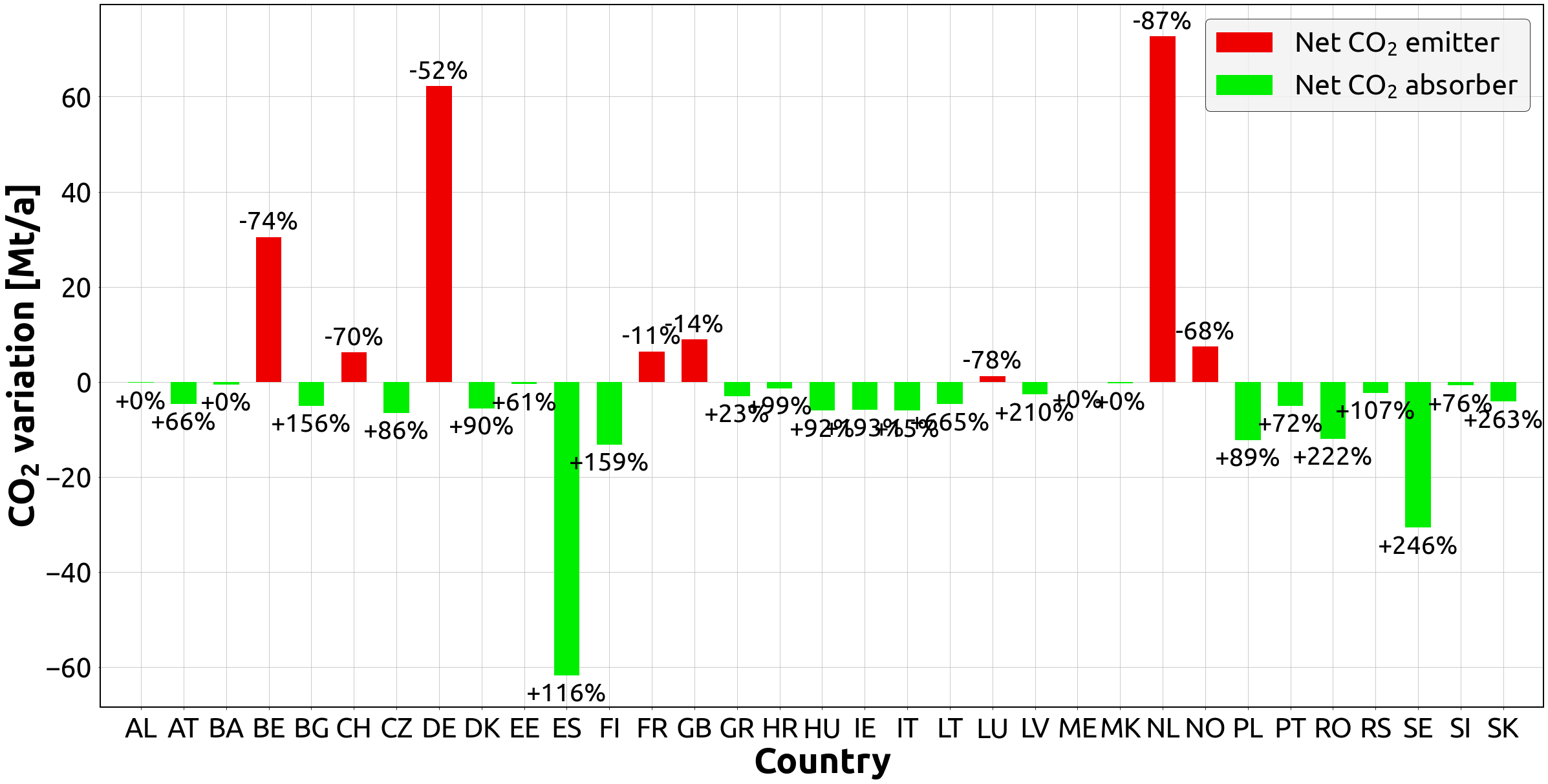
Figure S6: In the global net-zero CO₂ emissions scenario, countries that emit more CO₂ than they capture are represented by red bars, while countries that capture more CO₂ than they emit are represented by green bars. The percentages on top of the red bars indicate how much CO₂ net emitter countries do not capture, compared to their own emission values. On the other hand, the percentages at the bottom of the green bars indicate how much additional CO₂ net absorber countries capture, compared to their own emission values.

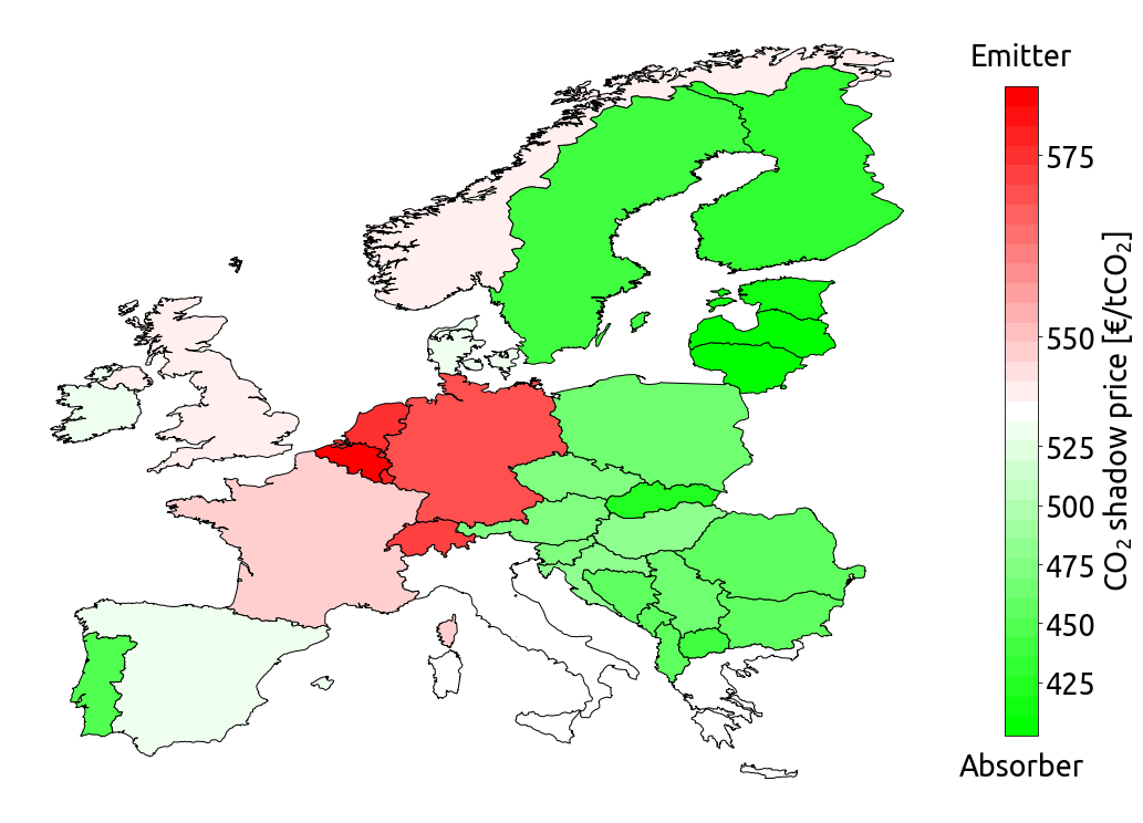
(a)

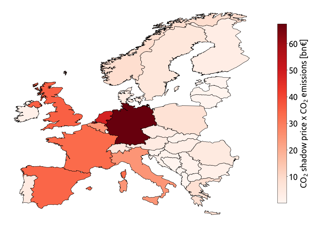
(b)

Figure S13: (a) CO₂ shadow price per country across Europe in the local net-zero CO₂ emissions scenario and (b) Product of CO₂ shadow price and CO₂ emissions per country across Europe in the local net-zero CO₂ emissions scenario. See Figure S7 for the amount of CO₂ emissions per country. As a reference, the CO₂ shadow price for the whole of Europe is set at 540 € per tonne of CO₂ in the global net-zero CO₂ emissions scenario.

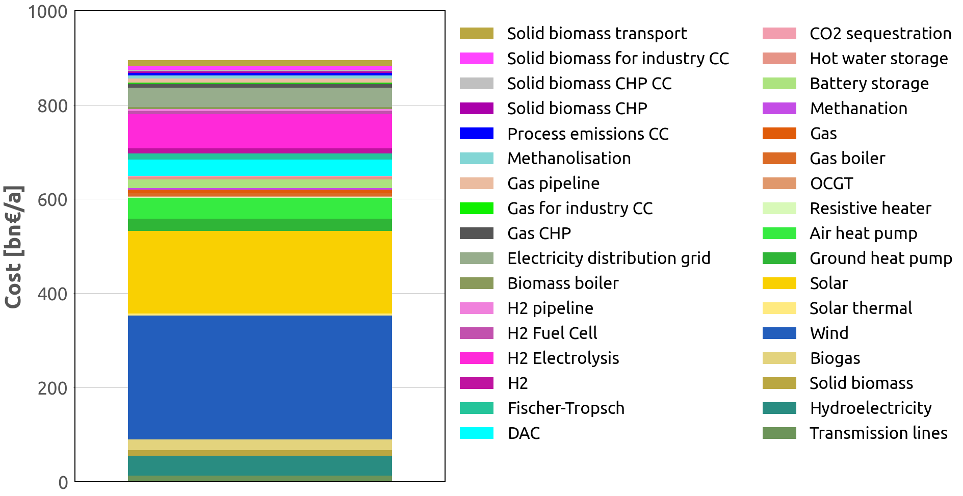
(a)

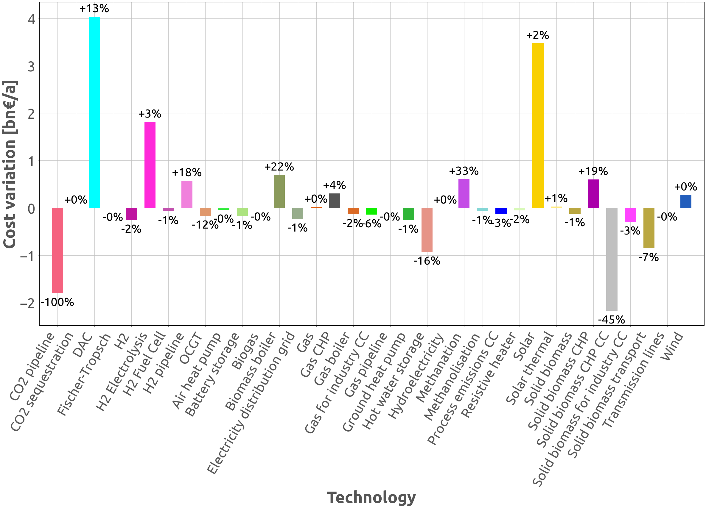
(b)

Figure S15: (a) Total system cost and technology configuration in the local net-zero CO₂ emissions scenario without a CO₂ network and (b) Cost variation per technology between the local net-zero CO₂ emissions scenario with a CO₂ network and the local net-zero CO₂ emissions scenario without a CO₂ network. The total cost increases by 0.6% when modelling a system without a CO₂ network compared to its counterpart equipped with such a network. Other than the differences in deployment levels, the technology configuration is the same in both types of systems.

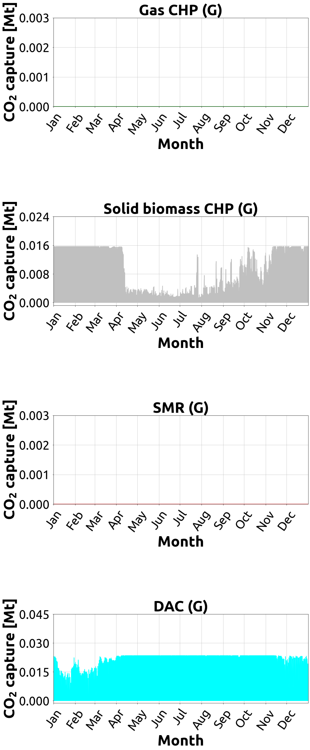
(a)

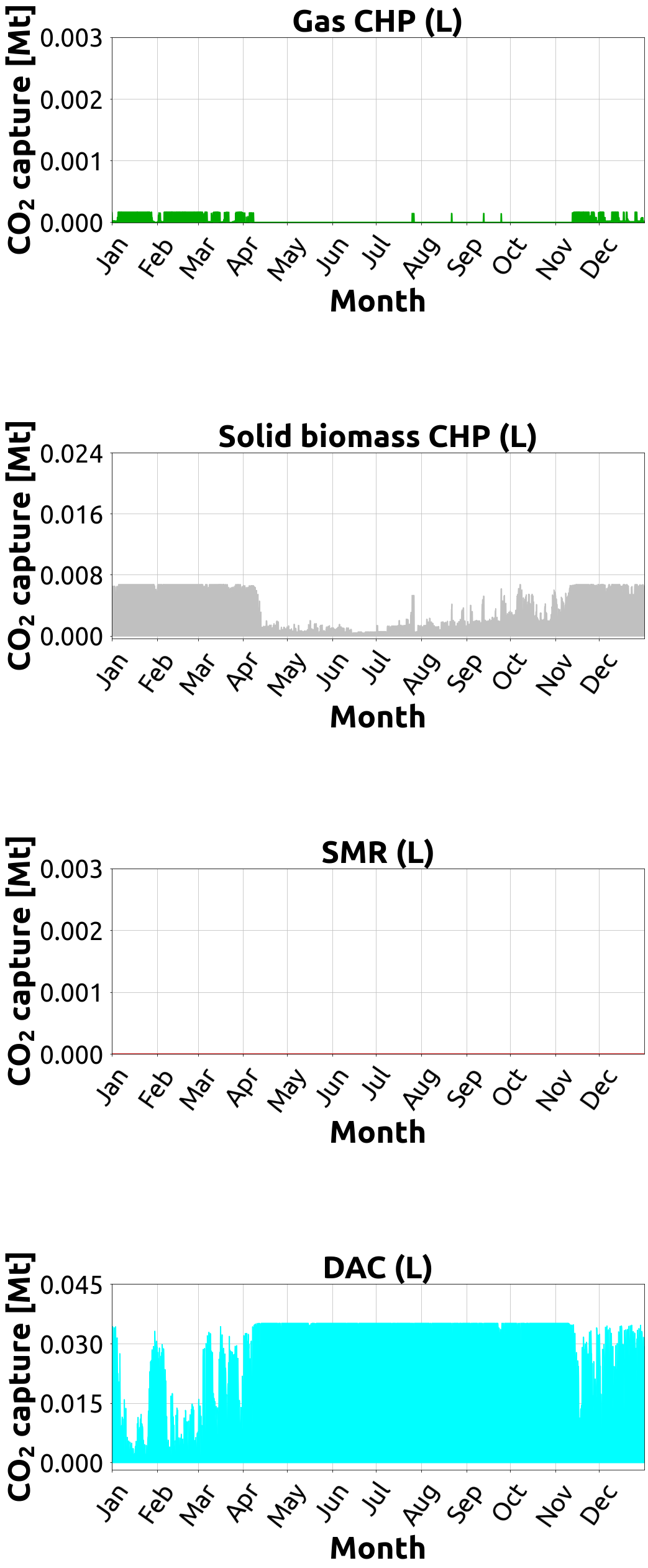
(b)

Figure S23: Temporal CO₂ capture from endogenous sources across all of Europe in (a) the global net-zero CO₂ emissions scenario and (b) the local net-zero CO₂ emissions scenario. Except for the absence of CO₂ captured from gas-based CHP units and SMR, which are not cost-competitive, the other two processes of capturing CO₂ exhibit a seasonal pattern. CO₂ captured from solid biomass-based CHP units increases in winter due to higher heat demand and decreases in summer. In contrast, CO₂ captured from DAC decreases in winter and increases in summer due to the availability of low-cost electricity.

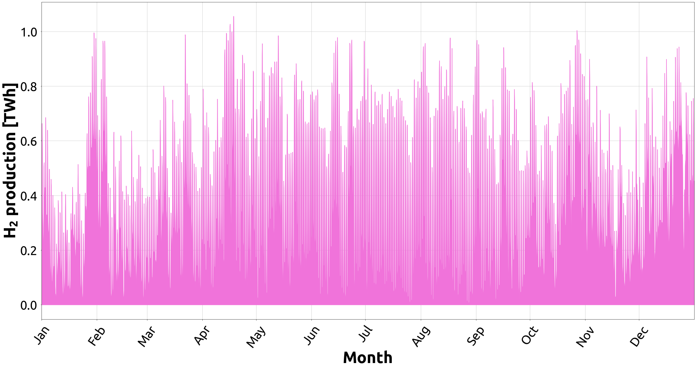
(a)

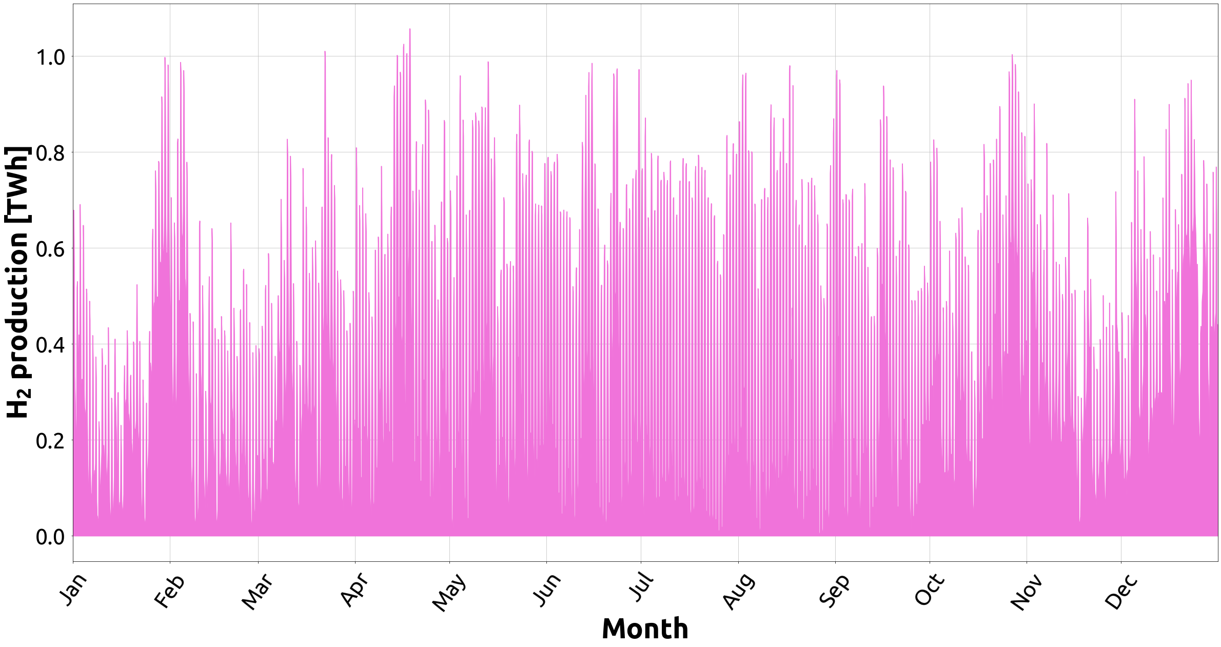
(b)

Figure S30: Temporal H₂ production across all of Europe in (a) the global net-zero CO₂ emissions scenario and (b) the local net-zero CO₂ emissions scenario. In both scenarios, the production of H₂ varies seasonally, with higher levels during the summer when there is an abundance of cost-effective energy to power H₂ electrolysis compared to winter.

Supplemental 3 Tables

Table S1: Characteristics assumptions about the main technologies used in PyPSA-Eur are based on the Energy System Technology Data for the year 2030. The comprehensive list of technologies is available at https://github.com/PyPSA/technology-data.

Technology	Parameter	Value
Battery storage	Investment	142 €/kWh
	Lifetime	25 years
Biogas	Investment	1539.62 €/kW
	Lifetime	20 years
	Efficiency	1 per unit
	FOM	12.84%/year
	Capture rate	0.98 per unit
Biomass boiler	Investment	649.3 €/kWth
	Lifetime	20 years
	Efficiency	0.86 per unit
	FOM	7.49%/year
CO2 pipeline	Investment	2000 €/tCO2/h/km
	Lifetime	50 years
	FOM	0.9%/year
CO2 sequestration	VOM	10 €/tCO2
Central air heat pump	Investment	856.25 €/kWth
	Lifetime	25 years
	Efficiency	3.6 per unit
	FOM	0.23%/year
	VOM	2.51 €/MWhth
Central gas boiler	Investment	50 €/kWth
	Lifetime	25 years
	Efficiency	1.04 per unit
	FOM	3.8%/year
	VOM	1 €/MWhth
Central ground heat pump	Investment	507.6 €/kWth
	Lifetime	25 years
	Efficiency	1.73 per unit
	FOM	0.39%/year
	VOM	1.25 €/MWhth
Central resistive heater	Investment	60 €/kWth
	Lifetime	20 years
	Efficiency	0.99 per unit
	FOM	1.7%/year
	VOM	1 €/MWhth
Central solar thermal	Investment	140000 €/1000m2
	Lifetime	20 years
	FOM	1.4%/year
Central water tank storage	Investment	0.54 €/kWh
	Lifetime	25 years
	FOM	0.55%/year
Decentral air heat pump	Investment	850 €/kWth
	Lifetime	18 years
	Efficiency	3.6 per unit
	FOM	3%/year
Decentral gas boiler	Investment	296.82 €/kWth
	Lifetime	20 years
	Efficiency	0.98 per unit
	FOM	6.69%/year
Decentral ground heat pump	Investment	1400 €/kWth
	Lifetime	20 years
	Efficiency	3.9 per unit
	FOM	1.82%/year
Decentral resistive heater	Investment	100 €/kWth
	Lifetime	20 years
	Efficiency	0.9 per unit
	FOM	2%/year
Decentral solar thermal	Investment	270000 €/1000m2
	Lifetime	20 years
	FOM	1.3%/year
Decentral water tank storage	Investment	18.38 €/kWh
	Lifetime	20 years
	FOM	1%/year
Direct air capture	Investment	6000000 €/tCO2/h
	Lifetime	20 years
	FOM	4.95%/year
	Electricity input	0.32 MWh/tCO2
	Heat input	2 MWh/tCO2
	Heat output	1 MWh/tCO2
Electricity distribution grid	Investment	500 €/kW
	Lifetime	40 years
	FOM	2%/year
Fischer-Tropsch	Investment	650711.26 €/MWFT
	Lifetime	20 years
	Efficiency	0.8 per unit
	FOM	3%/year
	Capture rate	0.98 per unit
Gas CHP	Investment	560 €/kW
	Lifetime	25 years
	Efficiency	0.41 per unit
	FOM	3.32%/year
	VOM	4.2 €/MWh
Gas CHP CC	Investment	560 €/kW
	Lifetime	25 years
	Efficiency	0.41 per unit
	FOM	3.32%/year
	VOM	4.2 €/MWh
	Capture rate	0.9 per unit
	CO2 intensity	0.2 tCO2/MWhth
	Electricity input	0.02 MWh/tCO2
	Heat input	0.72 MWh/tCO2
	Heat output	0.72 MWh/tCO2
Gas for industry CC	Investment	2600000 €/tCO2/h
	Lifetime	25 years
	FOM	3%/year
	Capture rate	0.9 per unit
	CO2 intensity	0.2 tCO2/MWhth
Gas storage	Investment	0.03 €/kWh
	Lifetime	100 years
	FOM	3.59%/year
H2 electrolysis	Investment	450 €/kWe
	Lifetime	30 years
	Efficiency	0.68 per unit
	FOM	2%/year
H2 fuel cell	Investment	1100 €/kWe
	Lifetime	10 years
	Efficiency	0.5 per unit
	FOM	5%/year
H2 pipeline	Investment	267 €/MW/km
	Lifetime	40 years
	FOM	3%/year
H2 storage tank type 1 + compr.	Investment	44.91 €/kWh
	Lifetime	30 years
	FOM	1.11%/year
H2 storage underground	Investment	2 €/kWh
	Lifetime	100 years
	FOM	0%/year
	VOM	0 €/MWh
HVAC overhead	Investment	432.97 €/MW/km
	Lifetime	40 years
	FOM	2%/year
HVDC overhead	Investment	432.97 €/MW/km
	Lifetime	40 years
	FOM	2%/year
HVDC submarine	Investment	471.16 €/MW/km
	Lifetime	40 years
	FOM	0.35%/year
Hydroelectricity	Investment	2208.16 €/kWel
	Lifetime	80 years
	Efficiency	0.9 per unit
	FOM	1%/year
Methanation (Sabatier)	Investment	628.6 €/MW${}_{CH_{4}}$
	Lifetime	20 years
	Efficiency	0.8 per unit
	FOM	3%/year
	Capture rate	0.98 per unit
Methane gas pipeline	Investment	79 €/MW/km
	Lifetime	50 years
	FOM	1.5%/year
Methanolisation	Investment	650711.26 €/MWMeOH
	Lifetime	20 years
	FOM	3%/year
OCGT	Investment	435.24 €/kW
	Lifetime	25 years
	Efficiency	0.41 per unit
	FOM	1.78%/year
	VOM	4.5 €/MWh
Offshore wind	Investment	1523.55 €/kWe
	Lifetime	30 years
	FOM	2.32%/year
	VOM	0.02 €/MWhel
Onshore wind	Investment	1035.56 €/kW
	Lifetime	30 years
	FOM	1.22%/year
	VOM	1.35 €/MWh
Process emissions CC	Investment	2600000 €/tCO2/h
	Lifetime	25 years
	FOM	3%/year
	Capture rate	0.9 per unit
SMR	Investment	493470.4 €/MW${}_{CH_{4}}$
	Lifetime	30 years
	Efficiency	0.76 per unit
	FOM	5%/year
SMR CC	Investment	572425.66 €/MW${}_{CH_{4}}$
	Lifetime	30 years
	Efficiency	0.69 per unit
	FOM	5%/year
	Capture rate	0.9 per unit
Solar	Investment	492.11 €/kWe
	Lifetime	40 years
	FOM	1.95%/year
	VOM	0.01 €/MWhel
Solid biomass	Investment	2209 €/kWel
	Lifetime	30 years
	Efficiency	0.47 per unit
	FOM	4.53%/year
Solid biomass CHP	Investment	3349.49 €/kWe
	Lifetime	25 years
	Efficiency	0.27 per unit
	FOM	2.87%/year
	VOM	4.58 €/MWhe
Solid biomass CHP CC	Investment	2700000 €/tCO2/h
	Lifetime	25 years
	FOM	3%/year
	Capture rate	0.9 per unit
	CO2 intensity	0.2 tCO2/MWhth
	Electricity input	0.02 MWh/tCO2
	Heat input	0.72 MWh/tCO2
	Heat output	0.72 MWh/tCO2
Solid biomass for industry CC	Investment	2600000 €/tCO2/h
	Lifetime	25 years
	FOM	3%/year
	Capture rate	0.9 per unit
	CO2 intensity	0.37 tCO2/MWhth

Table S2: Solid biomass transportation cost per country. The costs are based on the JRC European TIMES Energy System Model (JRC-EU-TIMES) and are available at https://data.jrc.ec.europa.eu/collection/id-00287.

Country	ISO	Cost [€/km/MWh]
Albania	AL	0.05521
Austria	AT	0.13646
Bosnia and Herzegovina	BA	0.05938
Belgium	BE	0.14063
Bulgaria	BG	0.06354
Switzerland	CH	0.17708
Czech Republic	CZ	0.08750
Germany	DE	0.13333
Denmark	DK	0.19063
Estonia	EE	0.08646
Spain	ES	0.11979
Finland	FI	0.14896
France	FR	0.14271
Great Britain	GB	0.14375
Greece	GR	0.11146
Croatia	HR	0.08021
Hungary	HU	0.07292
Ireland	IE	0.13333
Italy	IT	0.13229
Lithuania	LT	0.07396
Luxembourg	LU	0.14583
Latvia	LV	0.08125
Montenegro	ME	0.06042
North Macedonia	MK	0.05104
The Netherlands	NL	0.14583
Norway	NO	0.16146
Poland	PL	0.07813
Portugal	PT	0.09271
Romania	RO	0.06250
Serbia	RS	0.05729
Sweden	SE	0.16146
Slovenia	SI	0.09792
Slovakia	SK	0.08333

Table S3: CO₂ underground sequestration potential per country. The potentials are based on the European CO₂ storage database (CO2StoP) and are available at https://energy.ec.europa.eu/publications/assessment-co2-storage-potential-europe-co2stop_en. The model limits the aggregated CO₂ sequestration potential across Europe to 2.1 Gt and only considers the offshore underground potential.

Country	ISO	Potential [MtCO2]
Albania	AL	0
Austria	AT	0
Bosnia and Herzegovina	BA	0
Belgium	BE	0
Bulgaria	BG	0.21
Switzerland	CH	0
Czech Republic	CZ	0
Germany	DE	41.09
Denmark	DK	603.56
Estonia	EE	0.65
Spain	ES	7.27
Finland	FI	0
France	FR	0
Great Britain	GB	1000
Greece	GR	121.97
Croatia	HR	0
Hungary	HU	0
Ireland	IE	18.89
Italy	IT	33.82
Lithuania	LT	0.36
Luxembourg	LU	0
Latvia	LV	33.37
Montenegro	ME	0
North Macedonia	MK	0
The Netherlands	NL	4.66
Norway	NO	13.43
Poland	PL	0.56
Portugal	PT	212.23
Romania	RO	0
Serbia	RS	0
Sweden	SE	8.23
Slovenia	SI	0
Slovakia	SK	0

Table S4: CO₂ shadow price per country in the local net-zero CO₂ emissions scenario. The prices are the result of solving the model and are referred to as dual values associated with each constraint in a linear programming problem. As a reference, the CO₂ shadow price for all of Europe is set at 540 € per tonne of CO₂ in the global net-zero CO₂ emissions scenario.

Country	ISO	Price [€/tCO2]
Albania	AL	455
Austria	AT	474
Bosnia and Herzegovina	BA	454
Belgium	BE	584
Bulgaria	BG	458
Switzerland	CH	571
Czech Republic	CZ	476
Germany	DE	569
Denmark	DK	535
Estonia	EE	412
Spain	ES	534
Finland	FI	435
France	FR	548
Great Britain	GB	542
Greece	GR	538
Croatia	HR	479
Hungary	HU	480
Ireland	IE	530
Italy	IT	536
Lithuania	LT	405
Luxembourg	LU	579
Latvia	LV	402
Montenegro	ME	456
North Macedonia	MK	436
The Netherlands	NL	575
Norway	NO	544
Poland	PL	461
Portugal	PT	446
Romania	RO	460
Serbia	RS	467
Sweden	SE	436
Slovenia	SI	477
Slovakia	SK	426

Table S5: Conversion from MWh of energy to tonnes of CO₂ content based on stoichiometric reactions and thermal content of energy carriers. A factor of 3.6 is used to convert MWh to gigajoules (GJ). The molecular mass of CO₂ is 44.01 g/mol. Solid biomass is assumed to be composed of 50% carbon (C).

Energy carrier	GJ per tonne of energy carrier (a)	Material molecular mass [g/mol] (b)	Tonnes of CO2 per MWh of energy carrier 3.6 / (a) * 44.01 / (b)
Solid biomass	18	12.01 (C)	0.3664
Methane gas	50	16.04 (CH4)	0.1976
Oil	44	14 (C12H23)	0.2572
Methanol	22.7	32.04 (CH3OH)	0.2178

References

- [1] E. Commission, D.-G. for Climate Action, Going climate-neutral by 2050 – A strategic long-term vision for a prosperous, modern, competitive and climate-neutral EU economy, Publications Office, 2019. doi:doi/10.2834/02074.
-
[2]
Climate Change 2022 - Mitigation of Climate Change: Working Group III Contribution to the Sixth Assessment Report of the Intergovernmental Panel on Climate Change, Cambridge University Press, 2023, p. 3–48.
doi:10.1017/9781009157926.001.
URL https://www.cambridge.org/core/books/climate-change-2022-mitigation-of-climate-change/summary-for-policymakers/ABC31CEA863CB6AD8FEB6911A872B321 -
[3]
E. Commission, Climate strategies and targets (2024).
URL https://climate.ec.europa.eu/eu-action/climate-strategies-targets_en -
[4]
E. Commission, Questions and Answers on the EU Industrial Carbon Management Strategy (2024).
URL https://ec.europa.eu/commission/presscorner/detail/en/qanda_24_586 -
[5]
L. J. Schwenk-Nebbe, M. Victoria, G. B. Andresen, M. Greiner, CO2 quota attribution effects on the European electricity system comprised of self-centred actors, Advances in Applied Energy 2 (2021) 100012.
doi:https://doi.org/10.1016/j.adapen.2021.100012.
URL https://www.sciencedirect.com/science/article/pii/S2666792421000056 -
[6]
T. T. Pedersen, M. S. Andersen, M. Victoria, G. B. Andresen, Using Modeling All Alternatives to explore 55% decarbonization scenarios of the European electricity sector, iScience 26 (5) (2023) 106677.
doi:10.1016/j.isci.2023.106677.
URL http://dx.doi.org/10.1016/j.isci.2023.106677 - [7] J. Strefler, N. Bauer, F. Humpenöder, D. Klein, A. Popp, E. Kriegler, Carbon dioxide removal technologies are not born equal, Environmental Research Letters 16 (07 2021). doi:10.1088/1748-9326/ac0a11.
-
[8]
N. Bauer, C. Bertram, A. Schultes, D. Klein, G. Luderer, E. Kriegler, A. Popp, O. Edenhofer, Quantification of an efficiency-sovereignty trade-off in climate policy, Nature 588 (7837) (2020) 261–266.
doi:10.1038/s41586-020-2982-5.
URL https://doi.org/10.1038/s41586-020-2982-5 -
[9]
M. Victoria, E. Zeyen, T. Brown, Speed of technological transformations required in Europe to achieve different climate goals, Joule 6 (5) (2022) 1066–1086.
doi:https://doi.org/10.1016/j.joule.2022.04.016.
URL https://www.sciencedirect.com/science/article/pii/S2542435122001830 - [10] F. Neumann, E. Zeyen, M. Victoria, T. Brown, The potential role of a hydrogen network in Europe, Joule 7 (07 2023). doi:10.1016/j.joule.2023.06.016.
- [11] F. Hofmann, C. Tries, F. Neumann, E. Zeyen, T. Brown, H2 and CO2 Network Strategies for the European Energy System (2024). arXiv:2402.19042.
-
[12]
M. Wetzel, H. C. Gils, V. Bertsch, Green energy carriers and energy sovereignty in a climate neutral European energy system, Renewable Energy 210 (2023) 591–603.
doi:https://doi.org/10.1016/j.renene.2023.04.015.
URL https://www.sciencedirect.com/science/article/pii/S0960148123004639 -
[13]
J. Hörsch, F. Hofmann, D. Schlachtberger, T. Brown, PyPSA-Eur: An open optimisation model of the European transmission system, Energy Strategy Reviews 22 (2018) 207–215.
doi:https://doi.org/10.1016/j.esr.2018.08.012.
URL https://www.sciencedirect.com/science/article/pii/S2211467X18300804 -
[14]
T. Brown, J. Hörsch, D. Schlachtberger, PyPSA: Python for Power System Analysis, Journal of Open Research Software 6 (4) (2018).
arXiv:1707.09913, doi:10.5334/jors.188.
URL https://doi.org/10.5334/jors.188 -
[15]
Technology Data for Generation of Electricity and District Heating, Tech. rep., Danish Energy Agency (2020).
URL https://ens.dk/en/our-services/projections-and-models/technology-data/technology-data-generation-electricity-and -
[16]
M. Victoria, K. Zhu, E. Zeyen, T. Brown, Energy System Technology Data (2020).
URL https://github.com/PyPSA/technology-data -
[17]
S. Pfenninger, Dealing with multiple decades of hourly wind and PV time series in energy models: A comparison of methods to reduce time resolution and the planning implications of inter-annual variability, Applied Energy 197 (2017) 1–13.
doi:https://doi.org/10.1016/j.apenergy.2017.03.051.
URL https://www.sciencedirect.com/science/article/pii/S0306261917302775 - [18] J. Hörsch, T. Brown, The role of spatial scale in joint optimisations of generation and transmission for European highly renewable scenarios (2017) 1–7doi:10.1109/EEM.2017.7982024.
-
[19]
C. E. Fleischer, Minimising the effects of spatial scale reduction on power system models, Energy Strategy Reviews 32 (2020) 100563.
doi:https://doi.org/10.1016/j.esr.2020.100563.
URL https://www.sciencedirect.com/science/article/pii/S2211467X20301164 -
[20]
B. U. Schyska, A. Kies, M. Schlott, L. von Bremen, W. Medjroubi, The sensitivity of power system expansion models, Joule 5 (10) (2021) 2606–2624.
doi:https://doi.org/10.1016/j.joule.2021.07.017.
URL https://www.sciencedirect.com/science/article/pii/S254243512100355X - [21] M. M. Frysztacki, G. Recht, T. Brown, A comparison of clustering methods for the spatial reduction of renewable electricity optimisation models of Europe, Energy Informatics 5 (1) (2022) Art.–Nr.: 4, 37.12.02; LK 01. doi:10.1186/s42162-022-00187-7.
-
[22]
F. Hofmann, J. Hampp, F. Neumann, T. Brown, J. Hörsch, atlite: A Lightweight Python Package for Calculating Renewable Power Potentials and Time Series, Journal of Open Source Software 6 (62) (2021) 3294.
doi:10.21105/joss.03294.
URL https://doi.org/10.21105/joss.03294 - [23] H. Hersbach, B. Bell, P. Berrisford, G. Biavati, A. Horányi, J. Muñoz Sabater, J. Nicolas, C. Peubey, R. Radu, I. Rozum, et al., ERA5 hourly data on single levels from 1979 to present, Copernicus climate change service (c3s) climate data store (cds) 10 (10.24381) (2018).
- [24] E. K. Gøtske, G. B. Andresen, F. Neumann, M. Victoria, Designing a sector-coupled European energy system robust to 60 years of historical weather data (2024). arXiv:2404.12178.
-
[25]
P. J. Coker, H. C. Bloomfield, D. R. Drew, D. J. Brayshaw, Interannual weather variability and the challenges for Great Britain’s electricity market design, Renewable Energy 150 (2020) 509–522.
doi:https://doi.org/10.1016/j.renene.2019.12.082.
URL https://www.sciencedirect.com/science/article/pii/S0960148119319548 -
[26]
ENTSOE, TYNDP 2018 (2018).
URL https://tyndp-data.netlify.app/tyndp2018 - [27] A. Pluta, W. Medjroubi, J. C. Diettrich, J. Dasenbrock, H.-P. Tetens, J. E. Sandoval, O. Lunsdorf, SciGRID_gas - Data Model of the European Gas Transport Network, in: 2022 Open Source Modelling and Simulation of Energy Systems (OSMSES), 2022, pp. 1–7. doi:10.1109/OSMSES54027.2022.9769122.
-
[28]
S. M. Smith, O. Geden, G. F. Nemet, M. J. Gidden, W. F. Lamb, C. Powis, R. Bellamy, M. W. Callaghan, A. Cowie, E. Cox, S. Fuss, T. Gasser, G. Grassi, J. Greene, S. Lück, A. Mohan, G. P. Müller-Hansen, F.and Peters, Y. Pratama, T. Repke, K. Riahi, F. Schenuit, J. Steinhauser, J. Strefler, J. M. Valenzuela, J. C. Minx, The State of Carbon Dioxide Removal - 1st Edition, Tech. rep., The State of Carbon Dioxide Removal (2023).
doi:10.17605/OSF.IO/W3B4Z.
URL https://doi.org/10.17605/OSF.IO/W3B4Z -
[29]
P. Ruiz, W. Nijs, D. Tarvydas, A. Sgobbi, A. Zucker, R. Pilli, R. Jonsson, A. Camia, C. Thiel, C. Hoyer-Klick, F. Dalla Longa, T. Kober, J. Badger, P. Volker, B. Elbersen, A. Brosowski, D. Thrän, ENSPRESO - an open, EU-28 wide, transparent and coherent database of wind, solar and biomass energy potentials, Energy Strategy Reviews 26 (2019) 100379.
doi:https://doi.org/10.1016/j.esr.2019.100379.
URL https://www.sciencedirect.com/science/article/pii/S2211467X19300720 -
[30]
Captura, Carbon Dioxide Removal Pathway: Ocean Health and MRV (2023).
URL https://capturacorp.com/wp-content/uploads/2023/10/Captura-Carbon-Dioxide-Removal-Pathway.pdf -
[31]
E. Union, European co2 storage database (2020).
URL https://setis.ec.europa.eu/european-co2-storage-database_en