Robust VAEs via Generating Process of Noise Augmented Data
Hiroo Irobe111Equally contributedDepartment of Mathematical and Computing Science,
Tokyo Institute of Technology,
2-12-1 Ookayama, Meguro-ku,
Tokyo,
152-8550,
Japan
Wataru Aoki∗Department of Mathematical and Computing Science,
Tokyo Institute of Technology,
2-12-1 Ookayama, Meguro-ku,
Tokyo,
152-8550,
Japan
Kimihiro Yamazaki
Fujitsu Limited,
4-1-1 Kamikodanaka, Nakahara-ku, Kawasaki-shi,
Kanagawa,
211-8588,
Japan
Yuhui Zhang
Department of Mathematical and Computing Science,
Tokyo Institute of Technology,
2-12-1 Ookayama, Meguro-ku,
Tokyo,
152-8550,
Japan
Takumi Nakagawa
Department of Mathematical and Computing Science,
Tokyo Institute of Technology,
2-12-1 Ookayama, Meguro-ku,
Tokyo,
152-8550,
Japan
RIKEN Center for Advanced Intelligence Project,
Nihonbashi 1-chome Mitsui Building, 15th floor, 1-4-1 Nihonbashi, Chuo-ku,
Tokyo,
103-0027,
Japan
Hiroki Waida
Department of Mathematical and Computing Science,
Tokyo Institute of Technology,
2-12-1 Ookayama, Meguro-ku,
Tokyo,
152-8550,
Japan
Yuichiro Wada
Fujitsu Limited,
4-1-1 Kamikodanaka, Nakahara-ku, Kawasaki-shi,
Kanagawa,
211-8588,
Japan
RIKEN Center for Advanced Intelligence Project,
Nihonbashi 1-chome Mitsui Building, 15th floor, 1-4-1 Nihonbashi, Chuo-ku,
Tokyo,
103-0027,
Japan
Takafumi Kanamori222Corresponding author; E-mail: kanamori@c.titech.ac.jpDepartment of Mathematical and Computing Science,
Tokyo Institute of Technology,
2-12-1 Ookayama, Meguro-ku,
Tokyo,
152-8550,
Japan
RIKEN Center for Advanced Intelligence Project,
Nihonbashi 1-chome Mitsui Building, 15th floor, 1-4-1 Nihonbashi, Chuo-ku,
Tokyo,
103-0027,
Japan
Abstract
Advancing defensive mechanisms against adversarial attacks in generative models is a critical research topic in machine learning. Our study focuses on a specific type of generative models - Variational Auto-Encoders (VAEs). Contrary to common beliefs and existing literature which suggest that noise injection towards training data can make models more robust, our preliminary experiments revealed that naive usage of noise augmentation technique did not substantially improve VAE robustness. In fact, it even degraded the quality of learned representations, making VAEs more susceptible to adversarial perturbations. This paper introduces a novel framework that enhances robustness by regularizing the latent space divergence between original and noise-augmented data. Through incorporating a paired probabilistic prior into the standard variational lower bound, our method significantly boosts defense against adversarial attacks. Our empirical evaluations demonstrate that this approach, termed Robust Augmented Variational Auto-ENcoder (RAVEN), yields superior performance in resisting adversarial inputs on widely-recognized benchmark datasets.
1 Introduction
Generative models, such as Variational Auto-Encoders (VAEs) [1], generative adversarial networks [2], normalizing flows [3], diffusion models [4], and autoregressive models [5], have garnered significant attention in machine learning research. These models are capable of generating novel content, including text [6], images [1], and videos [7]. In the case of VAEs, generation is achieved through an auto-encoder, with the training objective being the maximization of a variational lower bound [1], hence its name. Recently, this methodology has been applied in drug discovery, particularly using a VAE-based model, cryoDRGN [8], for reconstructing continuous distributions of 3D protein structures from 2D images collected by electron microscopes.
Existing research [9] and [10] show that the original VAE [1] struggles with reconstruction and downstream classification under adversarial inputs. Various methods [9, 11, 10, 12, 13] have been proposed to address these issues. In [9], it was observed that the original VAE lacked robustness against inputs outside the empirical data distribution. Subsequently, they formulated a modified variational lower-bound that incorporates these inputs, aiming to construct a more robust VAE. In downstream classification tasks, their method showed remarkable efficacy.
In study [10], a Markov chain Monte Carlo sampling approach was employed during the inference steps to counteract adversarial inputs, by shifting the latent representation of the attacks back to more probable regions within the posterior distribution. This technique [10] effectively improved the model’s robustness.
Besides the above successful approaches, another strategy, presented in [14], involves using additive random noise on original data to fortify classifiers against adversarial inputs in supervised learning, as supported by theoretical and experimental evidence. Influenced by these findings, we conducted preliminary experiments on the MNIST dataset [15], comparing the performance of the following two VAE configurations in downstream classification tasks [9]:
(A)
a VAE trained exclusively on original dataset ,
(B)
a VAE trained on both original and corresponding noisy dataset , where , and is random Gaussian noise: .
We assessed performance using the encoder’s linear classification accuracy against adversarial inputs [9]. However, the results showed no significant improvement in classification accuracies, suggesting that the
naive usage of the noisy data in (B) was insufficient to enhance the original VAE’s robustness.
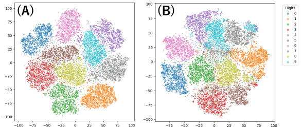
Figure 1:
t-SNE visualization of latent variables by trained VAE on test MNIST: (A) trained on original MNIST training data , (B) trained on both original and noisy data , where . Colors denote class labels on the top-right.
To understand the cause of the failure, we analyzed the latent variables and , outputs of the encoder on inputs and respectively; the t-SNE visualization [16] of Figure 1 also shows that the representations of (B) are similar to (A).
We then discovered unexpected behavior in the VAE under condition (B): the average squared Euclidean distance between and was larger compared to (A), despite the inclusion of noisy data in (B)’s training dataset; see the first and second columns in Table 1.
See further details of our preliminary experiments in Appendix C.1.
We hypothesize that this failure partly stems from the distant representation of the pair , which hampers the enhancement of robustness. In this study, we aim to construct a robust VAE by
bringing
the variables and closer together in the latent space. To achieve this, we integrated a probabilistic model of the paired variables [17] into the prior of the original variational lower-bound [1]. This model illustrates the generation mechanism of the paired variables from original data.
Our three key contributions are summarized below:
1)
We derived a novel variational lower-bound by incorporating the generating process for a robust VAE. The proposed bound is computationally efficient due to its closed-form structure, and its simplicity allows seamless integration with existing VAE extensions like -VAE [18] and VaDE [19], as well as methods like [10] and [13] to further enhance the robustness. We name our method the Robust Augmented Variational auto-ENcoder (RAVEN).
2)
Our analysis of this bound reveals that it is a generalization of the original bound [1], and provides an intuitive understanding of how it effectively narrows the distance between the paired representational variables .
3)
We empirically prove that our hypothesis is correct by results of our numerical experiments: RAVEN shows superior resilience against various adversarial attacks across common datasets without compromising on reconstruction quality. The superior performance represents a significant advancement in the field, enhancing both the robustness and versatility of VAEs.
Table 1:
Mean std on , where (resp. ) is representation of original MNIST test data (resp. the corresponding noisy data ), obtained by an encoder. "VAE" and "VAE (noise)" correspond to (A) and (B).
VAE
VAE (noise)
Ours
2 Related Work
In Section 2.1, we review details of the original VAE [1], which serves as a foundational method for our study.
Subsequently, in Section 2.2, we briefly review existing methods to build a robust VAE [12] and [13], as introduced at the second paragraph of Section 1. At last, in Section 2.3, we describe details of the Smooth Encoder (SE) [9], given its relative similarity to our proposed method. The distinctions between this method and our own to ours are clarified at the conclusion of this section.
In the following, for a random variable ,
let denote a multivariate Gaussian distribution with mean and variance matrix :
(1)
and we use notation .
2.1 Variational Auto-Encoder
The VAE stands out as a widely recognized unsupervised generative model, based on an auto-encoder architecture. The auto-encoder is bifurcated into two components: an encoder and the decoder , where and are a set of the trainable parameters.
Given a data , the encoder returns to define the latent variable by , where is the Hadamard product and is a -dimensional random vector, whose distribution is a unit Gaussian . The two symbols respectively express the zero mean vector and the variance-covariance matrix defined by an identity matrix, respectively. By the definition, , .
The auto-encoder is trained under an objective that maximizes the log-likelihood . Since the direct maximization is intractable, the authors of [1] proposed the variational lower-bound to indirectly maximize , where , is a likelihood defined by the decoder , and is the prior distribution. The lower-bound has a form of
(2)
where is the approximated posterior distribution defined by . The symbol means the Kullback-Leibler (KL) divergence. In the original VAE, the normal Gaussian is set to the prior, and the KL term can be expressed as a closed form [1]. Usually, the reconstruction term is approximately computed by a sample from the approximated posterior.
2.2 Existing Methods for Building Robust VAE
The researchers in [12] introduced the regularization method called total correlation to the original VAE, which serves to smoothen the embeddings in the latent space. Additionally, by introducing a hierarchical VAE, it was able to achieve both adversarial robustness and high reconstruction quality.
The authors of [13] suggest that VAEs do not consistently encode typical samples generated from their own decoder. They propose an alternative construction of the VAE with a Markov chain alternating between encoder and decoder, to enforce their consistency. Their method is reported to perform well in downstream classification tasks with adversarial inputs.
2.3 Smooth Encoder
As briefly mentioned in Section 1, the authors of [9] experimentally found that the original VAE was not robust against an input out of the the empirical distributional support. To solve the problem,
they proposed SE. This method assumes that the types of future attacks are known beforehand, thereby generating adversarial data from the original data tailored to these expected attacks. The method then employs a regularization to ensure the proximity between the representations of the original and the adversarial data.
This subsequently leads to a notable minimization of the entropy-regularized Wasserstein distance across the data representations. In SE’s framework, the derivation of a lower bound on the joint distribution of plays a crucial role, leading to a corresponding lower bound on the log-likelihood by integrating out .
In contrast to SE, our method is not reliant on foreknowledge of attack types, thus simplifying its computational process and eliminating the iterative gradient calculations required for creating adversarial data in SE. Additionally, our method is based on a variational lower bound directly on the joint distribution over the augmented data pair, as we will soon discuss.
3 Proposed Method
Let and be two augmented data instances generated from the original data . The joint distribution of this pair, denoted as , is assumed to have the following distribution [17]:
(3)
where
is the original data distribution, and
is the augmented data distribution conditioning on .
Similarly to the original VAE objective in Eq.(2), we consider a variational lower-bound of log-likelihood of the joint distribution over , as follows:
(4)
where are the corresponding latent variables to .
Inspired by the formulation presented in Eq.(3), we reconsider the generative process of the augmented data from the latent space perspective. We assume that, the corresponding latent variables, and , follow some conditional distribution given the original one . By adopting Gaussian distributions for , we achieve a closed-form derivation for Eq.(4). Our construction of a robust VAE will be based on the maximization of the novel lower bound.
Definition 1.
(Variant of Example 3.8 in [17])
The prior in Eq.(4) is given by
(5)
where , , and .
Note that we can recover Definition 1 by setting a normal Gaussian to the original data distribution of Example 3.8 in [17].
Assume the independence for of Eq.(4) as follows: , i.e., ; see the definitions of and in Section 2.1.
Then, \scriptsize2⃝ of Eq.(4) can be written as a closed form:
(7)
where .
Moreover, assume that .
Then, based on \scriptsize2⃝ of Eq.(7),
of Eq.(4) is equal to
(8)
The proof sketch is given in Section 3.2.
We also derived the variational lower bound of Eq.(4) in the case that of Definition 1 is the Gaussian mixture model; see Appendix B.
Remark 1.
We remark the connection between our proposed bound in Theorem 1 and the standard bound Eq.(2).
We select a "typical" input data for so that , and set . Disregarding constants that do not depend on network parameters or the input , the KL term of Eq.(4) simplifies to , aligning with the KL term from the standard VAE in Eq.(2).
Remark 2.
Regarding \scriptsize3⃝ in Eq.(7) - the terms related to the mean vectors and outputted by the encoder, when : is substantially less than in terms of e.g., maximum eigenvalues, it follows that . Consequently, the first term predominantly enforces and to converge. Furthermore, as shown in the following proposition, \scriptsize3⃝ enables the model to learn the appropriate distance for representations from the origin.
Proposition 2.
The term \scriptsize3⃝ in Eq.(7) can further be derived as
(9)
See the proof in Appendix A.3. In the right hand of Eq.(9), the first and second terms force both and to be the zero vector, while the last term keeps these vectors away and avoid to contract to the zero vector. Thus, the model has to learn to balance the two.
(Corollary 3.2b.1 of [20])
Consider the random variable , whose mean and the variance matrix are and , respectively. For a symmetric matrix , the following equation holds:
. Then, with a constant vector , the following holds: .
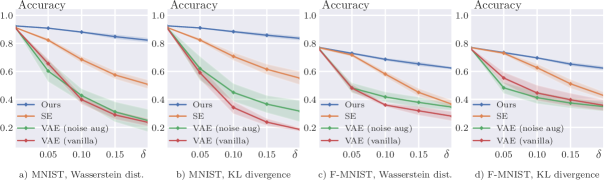
Figure 2: Attack budget (horizontal axis) versus classification accuracy (vertical axis) on MNIST (a, b) and Fashion-MNIST (c, d) datasets. Our proposed method (blue) significantly outperforms baseline methods under severe adversarial attacks, and is on par with them as the adversarial signal vanishes. Shaded area indicates standard derivations over 5 runs.
Lemma 2.
For the two -dimensional multivariate normal distributions and ,
consider the cross-entropy . Then, it is written as
.
Additionally, for the -dimensional normal distribution , the Shannon entropy of , i.e., is written as .
Lemma 2 can be immediately proved by using Lemma 1, as shown in Appendix A.1.
In Eq.(4), by the definition of the KL divergence, the part \scriptsize2⃝ equals to
where means the Shannon entropy. Moreover, from Proposition 1, the part \scriptsize4⃝ is decomposed into the summation of Eq.(11) and Eq.(12). Finally, by applying Lemma 2 to \scriptsize5⃝, we obtain Eq.(7).
4 Numerical Experiments
Toward a practical evaluation of our method, we conducted experiments on MNIST [15] and Fashion MNIST [21] (F-MNIST) datasets while keeping our focus on model robustness.
The efficiency of our proposed model against adversarial attacks is highlighted in those experiments.
We report the corresponding details and results in the following.
4.1 Experiment Setup
4.1.1 Adversarial attacks
An adversarial attack is some carefully crafted alternations of the input data,
designed to mislead models into yielding erroneous predictions or classifications [22].
In our study, we focus on small perturbations on the input data that can provoke substantial deviations in representations.
Given attackers an accessible encoder model , and a specified attack budget ,
their goal is to induce the maximum change in model representations,
measured by some dissimilarity function :
(13)
In Eq.(13), we adopted hence the maximum norm . takes Wasserstein distance or KL divergence.
Therefore, throughout our experiments, there are 2 types of adversarial attacks being considered in total.
To optimize Eq.(13) w.r.t. , we apply the Projected Gradient Descent (PGD) algorithm with 50 iterations and stepsize , maximizing either Wasserstein distance or KL divergence between the encoded representation posteriors.
4.1.2 Experiment protocols
Referring the experiment protocols in [9], our experiments with adversarial attack proceeds as follows:
As the first step, we train the VAE independently of downstream tasks until model converges.
The encoder and the decoder are symmetric 3-layer MLPs with PReLU activations [23], without normalization layers.
The model is trained with RAdam optimizer [24] and learning rate 0.001.
We then freeze the encoder parameters, and extract representation for each training data .
The mean given by the encoder will be the representation :
(14)
Secondly, following the common linear evaluation method, we train a simple linear classifier on the pairs of fixed representations and corresponding labels via the cross-entropy loss.
Finally, we assess model robustness by generating adversarial examples for each test instance using Eq.(13).
We report their test-set classification accuracy under such attacks in our results.
Table 2:
Reconstruction performance results of proposed method and various baselines.
Numbers indicate mean and standard derivations over 5 runs.
The best performance is in bold font. Results with in Figure 2 are reported in this table.
model
Accuracy (%)
MSE
FID
MNIST
VAE
91.45 0.26
862.114 10.96
21.766 0.27
VAE (noise)
91.84 0.45
916.383 15.43
23.990 0.86
SE
91.44 0.19
876.454 10.82
22.434 0.70
Ours
92.49 0.51
795.946 16.01
20.636 0.49
F-MNIST
VAE
76.33 0.89
915.934 10.69
50.338 0.85
VAE (noise)
76.71 0.58
953.350 17.46
52.151 0.78
SE
77.02 0.87
963.828 19.64
52.896 1.36
Ours
77.20 0.18
821.254 14.84
45.751 0.54
4.2 Results and Discussions
Following the protocols established in Section 4.1,
we compare our method with various baselines in practice, including vanilla and noise-augmented VAEs (for definitions of vanilla and noise-augmented, see (A) and (B) in Section 1) and SE [9] on MNIST and F-MNIST datasets. In our method, the augmented pair in Eq.(3) is constructed as , where . We set the variance in Definition 1 to for F-MNIST and for MNIST. Finally, we adopt cross-entropy metric for the first and second terms in Eq.(8) like the authors of [1]. See Appendix C.2 for details of hype-parameter tuning.
The results are shown in Figure 2 and Table 2.
As shown in the above results, for vanilla and noise-augmented VAEs, their improvements in robustness under adversarial attacks are limited.
Across datasets and different attacks, our method consistently outperforms SE in adversarial accuracy.
Especially, the performance of SE is highly impacted by strong adversarial attacks in F-MNIST, a relatively complex dataset, while our method is able to sustain its performance under such circumstances, offering robust representations.
In Table 2, we also report the reconstruction quality in pixel-wise Mean Square Error (MSE) as in [9] and Fréchet Inception Distance (FID) [25], which captures a deep distance between the ground-truth (clean) images and reconstructed ones. Although SE and noise-augmented VAEs suffer a slight decline in reconstruction fidelity—which can be attributed to their training on altered data and subsequent testing on clean data—our method appears immune to this trend.
Finally, we emphasize that distance of the paired representation are well improved compared to VAE and VAE (noise) in Table 1, suggesting our hypothesis introduced in Section 1 is correct.
5 Conclusion and Future Work
Our robust VAE, RAVEN, was proposed based on a novel variational bound via our hypothesis. We empirically confirm that the hypothesis is correct by RAVEN’s superior resilience against adversarial attacks. One of our future work is to further investigate our method theoretically and experimentally.
Acknowledgment
TK was partially supported by JSPS KAKENHI Grant Number 17H00764, 19H04071, and 20H00576.
Appendix A Lemmas and Propositions
Lemma 3.
Let and be the positive definite symmetric matrix. Then, the following equation holds: .
Proof.
∎
Proposition 3.
The product of the two density functions can be written as
where
.
Let us consider the case that in Definition 1 is defined by a Gaussian Mixture Model (GMM): .
For the definition of , see Eq.(1), and is the -th wight satisfying . The set is trainable, and it is denoted by .
Then, the prior in Definition 1, takes on the form of
Appendix C Further Details of Numerical Experiments
Let and denote -th original data in training dataset and -th original data in test dataset, respectively. In addition, let and , where (resp. ) denotes the number of training (resp. test) data points.
C.1 Preliminary Experiments
Using the original MNIST dataset [15],
we firstly evaluated the performance of the following two trained model:
(A)
a VAE trained by ,
(B)
a VAE trained by , where , and is -th random Gaussian noise.
The dimension of the latent space was ten for both VAEs, and both architectures (encoder and decoder) were the exactly same as described at the beginning of Section 4.1.2.
Additionally, with the original MNIST.
Let
(resp. ) denote the trained encoder of (A) (resp. (B)).
As shown in a) and b) of Figure 2, the accuracies of (A) and (B) were almost the same.
We then investigated the following two sets of the latent variables: and , where
and . In Figure 1, the t-SNE visualization of and are shown in (A) and (B), respectively.
Consider the set
on .
Then, the average and std over for (A) and (B) are shown in the first and second column in Table 1.
C.2 Hyper-Parameter Tuning and Model Architecture
In Section 4, we fixed the dimension of the latent space to for all methods. In addition, the hyper-parameters in all the existing methods were sufficiently tuned in our preliminary experiments using both MNIST and F-MNIST.
For our method, Raven, the primary hyperparameter is set to be . We explored a range for and found the best performing for F-MNIST and for MNIST, based on the metrics described at the end of Section 4.1.2.
In our experiments, we used a fully connected feed-forward neural network with layers arranged as (encoder), (decoder) with PReLU activation functions [23].
For SE, the key hyperparameter is , which controls the coupling strength for the regularized Wasserstein distance between the latent representations of the original data points and adversarial data points. From
, we found performs the best for MNIST and for F-MNIST.
References
[1]
D. P. Kingma and M. Welling, “Auto-encoding variational bayes,” in
International Conference on Learning Representations, 2014. [Online].
Available: http://arxiv.org/abs/1312.6114
[2]
I. Goodfellow, J. Pouget-Abadie, M. Mirza, B. Xu, D. Warde-Farley, S. Ozair,
A. Courville, and Y. Bengio, “Generative adversarial nets,” in
Advances in Neural Information Processing Systems, Z. Ghahramani,
M. Welling, C. Cortes, N. Lawrence, and K. Weinberger, Eds., vol. 27. Curran Associates, Inc., 2014. [Online].
Available:
https://proceedings.neurips.cc/paper_files/paper/2014/file/5ca3e9b122f61f8f06494c97b1afccf3-Paper.pdf
[3]
D. Rezende and S. Mohamed, “Variational inference with normalizing flows,” in
Proceedings of the 32nd International Conference on Machine Learning,
ser. Proceedings of Machine Learning Research, F. Bach and D. Blei, Eds.,
vol. 37. Lille, France: PMLR, 07–09
Jul 2015, pp. 1530–1538. [Online]. Available:
https://proceedings.mlr.press/v37/rezende15.html
[4]
Y. Song, J. Sohl-Dickstein, D. P. Kingma, A. Kumar, S. Ermon, and B. Poole,
“Score-based generative modeling through stochastic differential
equations,” in International Conference on Learning Representations,
2021. [Online]. Available: https://openreview.net/forum?id=PxTIG12RRHS
[5]
A. van den Oord, N. Kalchbrenner, and K. Kavukcuoglu, “Pixel recurrent neural
networks,” in Proceedings of The 33rd International Conference on
Machine Learning, ser. Proceedings of Machine Learning Research, M. F.
Balcan and K. Q. Weinberger, Eds., vol. 48. New York, New York, USA: PMLR, 20–22 Jun 2016, pp. 1747–1756.
[Online]. Available: https://proceedings.mlr.press/v48/oord16.html
[6]
H. Touvron, T. Lavril, G. Izacard, X. Martinet, M.-A. Lachaux, T. Lacroix,
B. Rozière, N. Goyal, E. Hambro, F. Azhar, A. Rodriguez, A. Joulin,
E. Grave, and G. Lample, “Llama: Open and efficient foundation language
models,” in arXiv, 2023.
[7]
U. Singer, A. Polyak, T. Hayes, X. Yin, J. An, S. Zhang, Q. Hu, H. Yang,
O. Ashual, O. Gafni, D. Parikh, S. Gupta, and Y. Taigman, “Make-a-video:
Text-to-video generation without text-video data,” in The Eleventh
International Conference on Learning Representations, 2023. [Online].
Available: https://openreview.net/forum?id=nJfylDvgzlq
[8]
E. D. Zhong, T. Bepler, B. Berger, and J. H. Davis, “CryoDRGN:
reconstruction of heterogeneous cryo-EM structures using neural networks,”
Nature Methods, vol. 18, no. 2, pp. 176–185, 2021.
[9]
T. Cemgil, S. Ghaisas, K. D. Dvijotham, and P. Kohli, “Adversarially robust
representations with smooth encoders,” in International Conference on
Learning Representations, 2020. [Online]. Available:
https://openreview.net/forum?id=H1gfFaEYDS
[11]
S. Eduardo, A. Nazabal, C. K. I. Williams, and C. Sutton, “Robust variational
autoencoders for outlier detection and repair of mixed-type data,” in
Proceedings of the Twenty Third International Conference on Artificial
Intelligence and Statistics, ser. Proceedings of Machine Learning Research,
S. Chiappa and R. Calandra, Eds., vol. 108. PMLR, 26–28 Aug 2020, pp. 4056–4066. [Online]. Available:
https://proceedings.mlr.press/v108/eduardo20a.html
[12]
M. J. Willetts, A. Camuto, T. Rainforth, S. Roberts, and C. C. Holmes,
“Improving VAEs’ robustness to adversarial attack,” in
International Conference on Learning Representations, 2021. [Online].
Available: https://openreview.net/forum?id=-Hs_otp2RB
[13]
T. Cemgil, S. Ghaisas, K. Dvijotham, S. Gowal, and P. Kohli, “The autoencoding
variational autoencoder,” in Advances in Neural Information Processing
Systems, H. Larochelle, M. Ranzato, R. Hadsell, M. Balcan, and H. Lin, Eds.,
vol. 33. Curran Associates, Inc.,
2020, pp. 15 077–15 087. [Online]. Available:
https://proceedings.neurips.cc/paper_files/paper/2020/file/ac10ff1941c540cd87c107330996f4f6-Paper.pdf
[14]
B. Li, C. Chen, W. Wang, and L. Carin, “Certified adversarial robustness with
additive noise,” in Advances in Neural Information Processing
Systems, H. Wallach, H. Larochelle, A. Beygelzimer, F. d'Alché-Buc, E. Fox, and R. Garnett, Eds., vol. 32. Curran Associates, Inc., 2019. [Online]. Available:
https://proceedings.neurips.cc/paper_files/paper/2019/file/335cd1b90bfa4ee70b39d08a4ae0cf2d-Paper.pdf
[15]
Y. Lecun, L. Bottou, Y. Bengio, and P. Haffner, “Gradient-based learning
applied to document recognition,” Proceedings of the IEEE, vol. 86,
no. 11, pp. 2278–2324, 1998.
[16]
L. van der Maaten and G. Hinton, “Visualizing data using t-sne,”
Journal of Machine Learning Research, vol. 9, no. 86, pp. 2579–2605,
2008. [Online]. Available:
http://jmlr.org/papers/v9/vandermaaten08a.html
[17]
J. Z. HaoChen, C. Wei, A. Gaidon, and T. Ma, “Provable guarantees for
self-supervised deep learning with spectral contrastive loss,” in
Advances in Neural Information Processing Systems, M. Ranzato,
A. Beygelzimer, Y. Dauphin, P. Liang, and J. W. Vaughan, Eds., vol. 34. Curran Associates, Inc., 2021, pp.
5000–5011. [Online]. Available:
https://proceedings.neurips.cc/paper_files/paper/2021/file/27debb435021eb68b3965290b5e24c49-Paper.pdf
[18]
I. Higgins, L. Matthey, A. Pal, C. Burgess, X. Glorot, M. Botvinick,
S. Mohamed, and A. Lerchner, “beta-VAE: Learning basic visual concepts
with a constrained variational framework,” in International Conference
on Learning Representations, 2017. [Online]. Available:
https://openreview.net/forum?id=Sy2fzU9gl
[19]
Z. Jiang, Y. Zheng, H. Tan, B. Tang, and H. Zhou, “Variational deep embedding:
An unsupervised and generative approach to clustering,” in Proceedings
of the Twenty-Sixth International Joint Conference on Artificial
Intelligence, IJCAI-17, 2017, pp. 1965–1972. [Online]. Available:
https://doi.org/10.24963/ijcai.2017/273
[20]
A. M. Mathai and S. B. Provost, Quadratic Forms in Random
Variables. CRC Press, 1992.
[21]
H. Xiao, K. Rasul, and R. Vollgraf, “Fashion-mnist: a novel image dataset for
benchmarking machine learning algorithms,” in arXiv, 2017.
[22]
I. Goodfellow, J. Shlens, and C. Szegedy, “Explaining and harnessing
adversarial examples,” in International Conference on Learning
Representations, 2015. [Online]. Available:
http://arxiv.org/abs/1412.6572
[23]
K. He, X. Zhang, S. Ren, and J. Sun, “Delving deep into rectifiers: Surpassing
human-level performance on imagenet classification,” in 2015 IEEE
International Conference on Computer Vision (ICCV), 2015, pp. 1026–1034.
[24]
L. Liu, H. Jiang, P. He, W. Chen, X. Liu, J. Gao, and J. Han, “On the variance
of the adaptive learning rate and beyond,” in International Conference
on Learning Representations, 2020. [Online]. Available:
https://openreview.net/forum?id=rkgz2aEKDr
[25]
M. Heusel, H. Ramsauer, T. Unterthiner, B. Nessler, and S. Hochreiter, “Gans
trained by a two time-scale update rule converge to a local nash
equilibrium,” in Advances in Neural Information Processing Systems,
I. Guyon, U. V. Luxburg, S. Bengio, H. Wallach, R. Fergus, S. Vishwanathan,
and R. Garnett, Eds., vol. 30. Curran
Associates, Inc., 2017. [Online]. Available:
https://proceedings.neurips.cc/paper_files/paper/2017/file/8a1d694707eb0fefe65871369074926d-Paper.pdf
[26]
J. R. Schott, Matrix analysis for statistics, 2nd ed. John Wiley & Sons, 2005.