Complexity of Quantum Harmonic Oscillator in External Magnetic Field

Abstract

In this paper, we investigate the circuit complexity of a quantum harmonic oscillator subjected to an external magnetic field. Utilizing the Nielsen approach within the thermofield dynamics (TFD) framework, we determine the complexity of thermofield double states as functions of time, temperature, and the external magnetic field. Our subsequent analysis reveals various features of this complexity. For instance, as temperature increases, the amplitude of complexity oscillations also rises, while at low temperatures, complexity stabilizes at a constant positive value. Furthermore, the magnetic field creates two distinct sectors: strong magnetic fields exhibit periodic complexity oscillations, whereas weak magnetic fields induce a beating effect. Finally, we confirm that the rate of complexity obeys the Lloyd bound.

1 Introduction

In recent years, there has been a growing interest in exploring the connections between information theory and fundamental physics within the framework of AdS/CFT correspondence. Since Ryu and Takayanagi’s conjecture [1, 2], which relates the entanglement entropy of a conformal field theory to the geometry of the corresponding anti-de Sitter spacetime, the interaction between gravity and entanglement has driven significant advancements in this field.

However, recent studies reveal that entanglement alone is insufficient to capture all features of the bulk theory [3, 4]. A notable example is the failure of entanglement entropy to describe the evolution of an eternal two-sided AdS black hole [5]. Specifically, when considering a thermofield double state (TFD) dual to such a black hole, the entanglement entropy of the TFD thermalizes [6], while the volume of the black hole’s interior continues to grow far beyond this thermalization time. To address this issue, Susskind and collaborators [4, 7, 8] introduced the notion of complexity, which can probe the growth of the black hole beyond the thermalization time of the entanglement entropy. Their original proposal posits that for an eternal black hole, the complexity is proportional to the spatial volume of the Einstein-Rosen bridge connecting the two boundaries.

Defining complexity within the holographic setup, however, involves subtleties that have led to various proposals, including complexity equals action (CA) [7], complexity equals volume (CV) [4], complexity equals spacetime volume (CV2.0) [8], and complexity equals anything [9, 10, 11, 12]. These conjectures aim to understand the quantum computational complexity of states in a boundary theory and their correspondence to gravitational descriptions in the bulk. The inherent subtleties are unavoidable due to similar ambiguities arising in complexity theory.

The notion of complexity originally stems from computer science [13, 14], where it defines the number of operations required to perform a specific task using a set of allowed simple operations. Building on this concept, various notions of complexity have emerged, such as quantum complexity [15, 16, 17, 18], time complexity [19], and holographic complexity [4, 7, 8]. Generalizing the concept of complexity to different systems is a nuanced task that involves making assumptions about these systems. For instance, in quantum computing, complexity is defined as the minimal number of simple unitary operations needed to transform one state into another.

Importantly, there is no single, universal definition of complexity; rather, a family of complexity measures exists that may be multiplicatively related under certain conditions. This idea aligns with Nielsen’s concepts of the geometry of computations, or complexity geometry [16, 17, 18]. To practically implement Nielsen’s approach, various methods and techniques have been developed, such as the covariance matrix method [20, 21, 22, 23], the Fubini-Study metric [24], and others [25, 26, 27].

Motivated by the significance of complexity in holography and other fields, we investigate the thermofield double (TFD) state of a quantum harmonic oscillator subjected to an external magnetic field. Specifically, we analyze the effects of the magnetic field on Nielsen complexity using the covariance matrix approach. This approach, however, is versatile and can be applied to study similar aspects in more general systems, including supersymmetric [28, 29, 30], noncommutative [31, 32, 33, 34], relativistic [35, 36, 37, 38], higher derivative [39, 40, 41, 42], and other [43, 44, 45] systems.

The structure of this paper is as follows: In Section 2, we quantize the harmonic oscillator in an external magnetic field and introduce the necessary bosonic creation and annihilation operators. In Section 3, we construct the time-evolved thermofield double (TFD) states of the system and represent them in a suitable operator form. In Section 4, we determine the thermal covariance matrix of the system. In Section 5, we compute the Nielsen complexity of the time-dependent TFD states and study its properties concerning temperature and the magnetic field. Furthermore, in Section 6, we calculate the complexity rate and demonstrate that it satisfies the Lloyd bound. Our results are summarized in Section 7.

2 Quantization of oscillator in an external magnetic field

In this section we consider the Schrödinger equation for a particle in an external field. We find the analytic solutions and show that the system reduces to two non-interacting simple harmonic oscillators.

2.1 The wave function

Let’s consider a spinless charged particle with mass $m$ in a homogeneous magnetic field $B$ oriented along the $z$-axis, equipped by an additional harmonic potential with frequency $\omega_{0}$. Restricting the motion to the $xy$-plane (with $p_{z}=0$), we obtain the following Hamiltonian:

$$H =\frac{1}{2m}\Big{(}\vec{p}-e\vec{A}\,\Big{)}^{2}+\frac{m\omega_{0}^{2}}{2}\big{(}x^{2}+y^{2}\big{)}$$

$$=\frac{1}{2m}\big{(}p_{x}^{2}+p_{y}^{2}\big{)}-\frac{eB}{2m}\big{(}xp_{y}-yp_{x}\big{)}+\frac{e^{2}B^{2}}{8m}\big{(}x^{2}+y^{2}\big{)}+\frac{m\omega_{0}^{2}}{2}\big{(}x^{2}+y^{2}\big{)}.$$ (2.1)

In this context, the magnetic potential $\vec{A}$ is considered in the symmetric gauge:

$$\vec{A}=\frac{B}{2}\left(\!\!\begin{array}[]{c}-y\\ x\\ 0\end{array}\!\!\right)\!.$$ (2.2)

Introducing the cyclotron frequency $\omega_{c}=\dfrac{eB}{m}$ and using the standard operator form of the momentum $p_{i}=-i\hbar\partial_{i}$, one has

$$H=-\frac{\hbar^{2}}{2m}(\partial_{x}^{2}+\partial_{y}^{2})+\frac{i\hbar\omega_{c}}{2}\big{(}x\partial_{y}-y\partial_{x}\big{)}+\frac{m}{8}\big{(}4\omega_{0}^{2}+\omega_{c}^{2}\big{)}\big{(}x^{2}+y^{2}\big{)}.$$ (2.3)

It is useful to change to polar coordinates:

$$x=\lambda\rho\cos\varphi,\quad y=\lambda\rho\sin\varphi,$$ (2.4)

where $\rho$ and $\varphi$ are dimensionless and $\lambda$ is a constant length parameter. The corresponding Laplacian and the angular momentum are of the form:

$$\Delta=\partial_{x}^{2}+\partial_{y}^{2}=\frac{1}{\lambda^{2}}\bigg{(}\partial_{\rho}^{2}+\frac{1}{\rho}\partial_{\rho}+\frac{1}{\rho^{2}}\partial_{\varphi}^{2}\bigg{)},\quad L_{z}=-i\hbar\big{(}x\partial_{y}-y\partial_{x}\big{)}=-i\hbar\partial_{\varphi}.$$ (2.5)

Hence, the Schrödinger equation $H\Psi(\rho,\varphi)=E\Psi(\rho,\varphi)$ yields:

$$\bigg{[}-\frac{\hbar^{2}}{2m\lambda^{2}}\bigg{(}\partial_{\rho}^{2}+\frac{1}{\rho}\partial_{\rho}+\frac{1}{\rho^{2}}\partial_{\varphi}^{2}\bigg{)}+\frac{i\hbar\omega_{c}}{2}\partial_{\varphi}+\frac{m}{8}\big{(}4\omega_{0}^{2}+\omega_{c}^{2}\big{)}\lambda^{2}\rho^{2}\bigg{]}\Psi=E\Psi.$$ (2.6)

The Hamiltonian is independent of $\varphi$, making the angular momentum along $\varphi$ a conserved quantity characterized by the quantum number $\ell$. This allows us to separate the variables using the following ansatz:

$$\Psi(\rho,\varphi)=e^{i\ell\varphi}R(\rho).$$ (2.7)

The latter leads to the following equation for the radial part $R(\rho)$:

$$R^{\prime\prime}(\rho)+\frac{1}{\rho}R^{\prime}(\rho)+\bigg{(}\frac{2m\lambda^{2}E}{\hbar^{2}}+\frac{m\omega_{c}\lambda^{2}\ell}{\hbar}-\frac{\ell^{2}}{\rho^{2}}-\frac{m^{2}}{4\hbar^{2}}\big{(}4\omega_{0}^{2}+\omega_{c}^{2}\big{)}\lambda^{4}\rho^{2}\bigg{)}R(\rho)=0.$$ (2.8)

Choosing $\lambda=\sqrt{\dfrac{2\hbar}{m\sqrt{4\omega_{0}^{2}+\omega_{c}^{2}}}}$ and changing variables to $\rho^{2}=r$, we obtain

$$rR^{\prime\prime}(r)+R^{\prime}(r)+\bigg{(}\frac{E}{\hbar\sqrt{4\omega_{0}^{2}+\omega_{c}^{2}}}+\frac{\omega_{c}\,\ell}{2\sqrt{4\omega_{0}^{2}+\omega_{c}^{2}}}-\frac{\ell^{2}}{4r}-\frac{r}{4}\bigg{)}R(r)=0.$$ (2.9)

This is a second-order differential equation of the Laguerre type, with the solution given by

$$R_{n,\ell}(r)=r^{\frac{\ell}{2}}e^{-\frac{r}{2}}L_{n}^{(\ell)}(r),$$ (2.10)

where $L_{n}^{(\ell)}(r)$ are the generalized Laguerre polynomials

$$L_{n}^{(\ell)}(r)=\frac{r^{-\ell}e^{r}}{n!}\frac{d^{n}}{dr^{n}}\Big{(}e^{-r}r^{n+\ell}\Big{)}=\sum\limits_{j=0}^{n}\frac{(-1)^{j}(n+\ell)!\,r^{j}}{j!(n-j)!(\ell+j)!},$$ (2.11)

Using the natural quantization condition $\frac{2E+\hbar\ell\omega_{c}}{2\hbar\sqrt{\omega_{c}^{2}+4\omega_{o}^{2}}}=n+\frac{\ell+1}{2}$ one finds the spectrum:

$$E_{n,\ell}=\hbar\sqrt{4\omega_{0}^{2}+\omega_{c}^{2}}\bigg{(}n+\frac{1}{2}\bigg{)}+\hbar\frac{\sqrt{4\omega_{0}^{2}+\omega_{c}^{2}}-\omega_{c}}{2}\,\ell,$$ (2.12)

where $n$ is the principal quantum number and $\ell$ is the magnetic quantum number. Due to the normalization of Laguerre polynomials,

$$\int_{0}^{\infty}r^{\ell}e^{-r}L_{n}^{(\ell)}(r)L_{m}^{(\ell)}(r)dr=\frac{\Gamma(n+\ell+1)}{n!}\delta_{nm},$$ (2.13)

and the property $n+\ell+1\geq 1$ for the gamma function, the quantum numbers take the following values:

$$n=0,1,2,...,\quad\ell=-n,-n+1,...,-1,0,1,2,...\,,$$ (2.14)

where $\ell$ is not bounded from above. Finally, we can write the complete wave function of the system:

$$\Psi_{n,\ell}(\rho,\varphi)=\frac{1}{\lambda}\sqrt{\frac{n!}{\pi(n+\ell)!}}\,e^{i\ell\varphi}\rho^{\ell}e^{-\frac{\rho^{2}}{2}}L_{n}^{(\ell)}\big{(}\rho^{2}\big{)},$$ (2.15)

with natural normalization given by

$$\lambda^{2}\int_{0}^{\infty}\!\!\!\int_{0}^{2\pi}\Psi_{n,\ell}^{*}(\rho,\varphi)\Psi_{n^{\prime},\ell^{\prime}}(\rho,\varphi)\,\rho\,d\rho\,d\varphi=\delta_{nn^{\prime}}\delta_{\ell\ell^{\prime}}.$$ (2.16)

2.2 Fock space

In order to construct the Fock space it is convenient to introduce the following creation and annihilation operators:

$$b=\frac{e^{-i\varphi}}{2}\bigg{(}\rho+\partial_{\rho}-\frac{i}{\rho}\partial_{\varphi}\bigg{)},\quad b^{\dagger}=\frac{e^{i\varphi}}{2}\bigg{(}\rho-\partial_{\rho}-\frac{i}{\rho}\partial_{\varphi}\bigg{)},$$

$$\!\!a=-\frac{e^{i\varphi}}{2}\bigg{(}\rho+\partial_{\rho}+\frac{i}{\rho}\partial_{\varphi}\bigg{)},\quad a^{\dagger}=-\frac{e^{-i\varphi}}{2}\bigg{(}\rho-\partial_{\rho}+\frac{i}{\rho}\partial_{\varphi}\bigg{)},$$ (2.17)

which satisfy the standard commutation relations:

$$[a,a^{\dagger}]=1=[b,b^{\dagger}],\quad[a,b]=0.$$ (2.18)

The action of these operators on the wave function (2.15) is given by:

$$a^{\dagger}\Psi_{n,\ell}=\sqrt{n+1}\,\Psi_{n+1,\ell-1},\quad b^{\dagger}\Psi_{n,\ell}=\sqrt{n+\ell+1}\,\Psi_{n,\ell+1},$$

$$a\Psi_{n,\ell}=\sqrt{n}\,\Psi_{n-1,\ell+1},\,\quad\qquad b\Psi_{n,\ell}=\sqrt{n+\ell\,}\,\Psi_{n,\ell-1}.$$ (2.19)

The application of $b^{\dagger}$ increases the number $\ell$ by one unit, while preserving $n$. The operator $a^{\dagger}$ simultaneously increases $n$ and decreases $\ell$ by one unit. We can simplify the notations by introducing a new shifted quantum number $k=n+\ell$. The relation between the existing wave function $\Psi$ and the new wave function $\Phi$ is given by:

$$\Psi_{n,k-n}=\Phi_{n,k}=\frac{(a^{\dagger})^{n}(b^{\dagger})^{k}}{\sqrt{n!k!}}\Phi_{0,0},\quad\Phi_{0,0}=\Psi_{0,0}.$$ (2.20)

Now the operators $a$ and $a^{\dagger}$ change only $n$, and the operators $b$ and $b^{\dagger}$ change only $k$:

$$a^{\dagger}\Phi_{n,k}=\sqrt{n+1}\,\Phi_{n+1,k},\qquad b^{\dagger}\Phi_{n,k}=\sqrt{k+1}\,\Phi_{n,k+1},$$

$$a\Phi_{n,k}=\sqrt{n}\,\Phi_{n-1,k},\qquad\qquad b\Phi_{n,k}=\sqrt{k}\,\Phi_{n,k-1}.$$ (2.21)

The energy in this case can be written in terms of the $n,k$ indices in the following form:

$$E_{n,k}=\hbar\omega_{1}\bigg{(}n+\frac{1}{2}\bigg{)}+\hbar\omega_{2}\bigg{(}k+\frac{1}{2}\bigg{)},\quad a^{\dagger}a\Phi_{n,k}=n\Phi_{n,k},\quad b^{\dagger}b\Phi_{n,k}=k\Phi_{n,k}.$$ (2.22)

Where the Hamiltonian reduces to the one of two non-interacting harmonic oscillators with frequencies

$$\omega_{1}=\frac{\sqrt{4\omega_{0}^{2}+\omega_{c}^{2}}+\omega_{c}}{2},\qquad\omega_{2}=\frac{\sqrt{4\omega_{0}^{2}+\omega_{c}^{2}}-\omega_{c}}{2}.$$ (2.23)

It is noted that $\omega_{1}\geq\omega_{2}$, with equality occurring only when the magnetic field is turned off $(\omega_{1}=\omega_{2}=\omega_{0},\,\omega_{c}=0)$.

3 Construction of TFD state

To construct the TFD we apply the standard approach. We double the Hilbert space to left/right sectors, which commute. In the $\Phi_{n,k}\equiv|n,k\rangle$ basis we can write the TFD state as:

$$|TFD\rangle =\frac{1}{\sqrt{Z}}\sum\limits_{n=0}^{\infty}\sum\limits_{k=0}^{\infty}e^{-\frac{\beta}{2}E_{n,k}}|n,k\rangle_{L}|n,k\rangle_{R}$$

$$=\frac{e^{-\frac{\beta\hbar}{4}(\omega_{1}+\omega_{2})}}{\sqrt{Z}}\exp\!\Big{(}e^{-\frac{\beta\hbar\omega_{1}}{2}}a^{\dagger}_{L}a^{\dagger}_{R}+e^{-\frac{\beta\hbar\omega_{2}}{2}}b^{\dagger}_{L}b^{\dagger}_{R}\Big{)}|0,0\rangle_{L}|0,0\rangle_{R},$$ (3.1)

where the energy $E_{n,k}$ is defined in Eq. (2.22). The operators $a_{L/R}$ and $b_{L/R}$ are defined in (2.2) and the partition function $Z$ follows from the normalization condition $\langle TFD|TFD\rangle=1$:

$$Z=\frac{e^{-\frac{\beta\hbar}{2}(\omega_{1}+\omega_{2})}}{\big{(}1-e^{-\beta\hbar\omega_{1}}\big{)}\big{(}1-e^{-\beta\hbar\omega_{2}}\big{)}}.$$ (3.2)

Expressing the TFD as a unitary operator acting on the vacuum, we find

$$|TFD\rangle=\exp\big{[}\alpha_{1}\big{(}a_{L}^{\dagger}a_{R}^{\dagger}-a_{L}a_{R}\big{)}+\alpha_{2}\big{(}b_{L}^{\dagger}b_{R}^{\dagger}-b_{L}b_{R}\big{)}\big{]}|0,0\rangle_{L}|0,0\rangle_{R},$$ (3.3)

where the coefficients $\alpha_{i}$, $i=1,2$, are written by [46]:

$$\tanh\alpha_{i}=e^{-\frac{\beta\hbar\omega_{i}}{2}}.$$ (3.4)

We can extend (3) and (3.3) to the time-dependent case in the following way:

$$|TFD(t)\rangle=\frac{1}{\sqrt{Z}}\sum\limits_{n=0}^{\infty}\sum\limits_{k=0}^{\infty}e^{-\frac{\beta}{2}E_{n,k}}\,e^{-\frac{i}{\hbar}E_{n,k}t}\,|n,k\rangle_{L}|n,k\rangle_{R}$$

$$=\exp\big{[}\alpha_{1}\big{(}e^{-i\omega_{1}t}a_{L}^{\dagger}a_{R}^{\dagger}-e^{i\omega_{1}t}a_{L}a_{R}\big{)}+\alpha_{2}\big{(}e^{-i\omega_{2}t}b_{L}^{\dagger}b_{R}^{\dagger}-e^{i\omega_{2}t}b_{L}b_{R}\big{)}\big{]}|0,0\rangle_{L}|0,0\rangle_{R},$$ (3.5)

where $\alpha_{i}$ are the same as in (3.4). One can introduce standard positions and momenta corresponding to the creation/annihilation operators by:

$$a_{L/R}=\sqrt{\frac{m\omega_{1}}{2\hbar}}\Bigg{(}X_{1\,L/R}+i\frac{P_{1\,L/R}}{m\omega_{1}}\Bigg{)},\quad b_{L/R}=\sqrt{\frac{m\omega_{2}}{2\hbar}}\Bigg{(}X_{2\,L/R}+i\frac{P_{2\,L/R}}{m\omega_{2}}\Bigg{)}.$$ (3.6)

A subsequent transformation to a light-cone basis yields:

$$X_{1\pm}=\frac{1}{\sqrt{2}}\big{(}X_{1L}\pm X_{1R}\big{)},\qquad P_{1\pm}=\frac{1}{\sqrt{2}}\big{(}P_{1L}\pm P_{1R}\big{)},$$

$$X_{2\pm}=\frac{1}{\sqrt{2}}\big{(}X_{2L}\pm X_{2R}\big{)},\qquad P_{2\pm}=\frac{1}{\sqrt{2}}\big{(}P_{2L}\pm P_{2R}\big{)}.$$ (3.7)

Hence, the argument of the unitary operator from (3.3) takes the form:

$$\alpha_{1}\big{(}a_{L}^{\dagger}a_{R}^{\dagger}-a_{L}a_{R}\big{)}+\alpha_{2}\big{(}b_{L}^{\dagger}b_{R}^{\dagger}-b_{L}b_{R}\big{)}=-i\alpha_{1}K_{1+}+i\alpha_{1}K_{1-}-i\alpha_{2}K_{2+}+i\alpha_{2}K_{2-},$$ (3.8)

where the $K_{i\,\pm}$ operators are defined as:

$$K_{i\pm}=\frac{1}{2\hbar}\big{(}X_{i\pm}P_{i\pm}+P_{i\pm}X_{i\pm}\big{)}.$$ (3.9)

This leads to the following form of the time-independent TFD:

$$|TFD\rangle=e^{-i\alpha_{1}K_{1+}}|0_{1+}\rangle\otimes e^{i\alpha_{1}K_{1-}}|0_{1-}\rangle\otimes e^{-i\alpha_{2}K_{2+}}|0_{2+}\rangle\otimes e^{i\alpha_{2}K_{2-}}|0_{2-}\rangle.$$ (3.10)

Therefore, in this basis, the unitary operator (3.3) completely decouples into four separate sectors, since all $K_{i\,\pm}$ commute with each other. Similarly we can calculate the new time-dependent unitary operator from (3) as:

$$\alpha_{1}\big{(}e^{-i\omega_{1}t}a_{L}^{\dagger}a_{R}^{\dagger}-e^{i\omega_{1}t}a_{L}a_{R}\big{)}+\alpha_{2}\big{(}e^{-i\omega_{2}t}b_{L}^{\dagger}b_{R}^{\dagger}-e^{i\omega_{2}t}b_{L}b_{R}\big{)}$$

$$=-i\alpha_{1}{K}_{1+}(t)+i\alpha_{1}{K}_{1-}(t)-i\alpha_{2}{K}_{2+}(t)+i\alpha_{2}{K}_{2-}(t),$$ (3.11)

where the time-dependent generalizations of the operators $K_{i}$ (3.9) can be expressed as:

$$\hat{K}_{i\pm}(t)=\frac{1}{2\hbar}\cos(\omega_{i}t)\big{(}X_{i\pm}P_{i\pm}+P_{i\pm}X_{i\pm}\big{)}+\frac{1}{2\hbar}\sin(\omega_{i}t)\bigg{(}m\omega_{i}X_{i\pm}^{2}-\frac{P_{i\pm}^{2}}{m\omega_{i}}\bigg{)}.$$ (3.12)

The time-dependent TFD state (3) now becomes:

$$|TFD(t)\rangle=e^{-i\alpha_{1}K_{1+}(t)}|0_{1+}\rangle\otimes e^{i\alpha_{1}K_{1-}(t)}|0_{1-}\rangle\otimes e^{-i\alpha_{2}K_{2+}(t)}|0_{2+}\rangle\otimes e^{i\alpha_{2}K_{2-}(t)}|0_{2-}\rangle,$$ (3.13)

which also decouples into four disjoint sectors.

4 Covariance matrix

In this section, we use the covariance matrix approach for computing Nielsen complexity, as introduced in [46]. This method is particularly useful for estimating complexity when both the initial and final states of the evolution are Gaussian, which is the case for the TFD state. The approach can be summarized in a few simple steps. First, represent the TFD state as generated by some unitary operator acting on the vacuum, $|\textrm{TFD}\rangle=U(t)|0\rangle$. Next, consider a set of generators $\xi^{r}$ that span all generators of the problem. Based on these generators, construct the covariance matrix:

$$G^{r,s}=\langle\psi|\xi^{r}\xi^{s}+\xi^{s}\xi^{r}|\psi\rangle,$$ (4.1)

where $\psi$ is an arbitrary state. Using this definition one can define the relative covariance matrix between two states by

$$\Delta=G_{T}.g_{R},$$ (4.2)

where $g_{R}$ is the inverse of the covariance matrix of the reference state, while $G_{T}$ is the covariance matrix of the target state. Finally, one can express the Nielsen complexity using the relative covariance matrix $\Delta$ via the Frobenius norm:

$$\mathcal{C}(t)=\frac{1}{2}\sqrt{\mathrm{Tr}(\ln\Delta)^{2}}.$$ (4.3)

Thus, the problem of finding the Nielsen complexity reduces to determining the eigenvalues of $\Delta$ (for details see [46] and references therein).

4.1 Covariance matrix for the time-independent TFD state

The covariance matrix for this problem can be expressed in terms of the set of operators $\vec{\xi}=\vec{\xi}_{1+}\oplus\,\vec{\xi}_{1-}\oplus\,\vec{\xi}_{2+}\oplus\,\vec{\xi}_{2-}=(X_{1+},P_{1+},X_{1-},P_{1-},X_{2+},P_{2+},X_{2-},P_{2-})^{T}$, where:

$$\vec{\xi}_{i\pm}=(X_{i\pm},P_{i\pm})^{T}.$$ (4.4)

The vacuum covariance matrix $O_{0}^{rs},(r,s=1,...,8)$ is written by

$$O_{0}^{rs}=\langle 0|\xi^{r}\xi^{s}|0\rangle=\frac{1}{2}\langle 0|\big{\{}\xi^{r},\xi^{s}\big{\}}|0\rangle+\frac{1}{2}\langle 0|\big{[}\xi^{r},\xi^{s}\big{]}|0\rangle=\frac{\hbar}{2}\big{(}G^{rs}_{0}+i\Omega^{rs}_{0}\big{)},$$ (4.5)

where one has $8\times 8$ block-diagonal matrices:

$$G_{0}=\left(\!\!\begin{array}[]{cccc}G_{01}&0&0&0\\ 0&G_{01}&0&0\\ 0&0&G_{02}&0\\ 0&0&0&G_{02}\\ \end{array}\!\!\right)\!,\quad\Omega_{0}=\left(\!\!\begin{array}[]{cccc}\Omega_{01}&0&0&0\\ 0&\Omega_{01}&0&0\\ 0&0&\Omega_{02}&0\\ 0&0&0&\Omega_{02}\\ \end{array}\!\!\right),$$ (4.6)

with $2\times 2$ submatrices given by

$$G_{0i}=\left(\!\begin{array}[]{cc}\frac{1}{m\omega_{i}}&0\\ 0&m\omega_{i}\\ \end{array}\!\right)\!,\quad\Omega_{0i}=\left(\!\!\begin{array}[]{cc}0&1\\ -1&0\\ \end{array}\!\!\right)\!.$$ (4.7)

The unitary operators $U_{i\pm}=e^{\mp i\alpha_{i}K_{i\pm}}$ act on the vacuum and create the thermal vacuum (3.10) such as:

$$|TFD\rangle\equiv|\alpha_{1},\alpha_{2}\rangle=U_{1+}|0_{1+}\rangle\otimes U_{1-}|0_{1-}\rangle\otimes U_{2+}|0_{2+}\rangle\otimes U_{2-}|0_{2-}\rangle.$$ (4.8)

It is convenient to introduce the matrix representations $\mathcal{U}_{i\pm}$ and $\mathcal{K}_{i\pm}$ of each of the operators above via $(a,b=1,2)$:

$$U_{i\pm}^{\dagger}\xi_{i\pm}^{a}U_{i\pm}=\mathcal{U}^{\,\,\,\,a}_{i\pm,b\,}\xi_{i\pm}^{b},\quad[iK_{i\pm},\xi_{i\pm}^{a}]=\big{(}\mathcal{K}_{i\pm}.\vec{\xi}_{i\pm}\big{)}^{a}=\mathcal{K}^{\,\,\,\,\,a}_{i\pm,b\,}\xi_{i\pm}^{b}.$$ (4.9)

Now we calculate the following product (there is no sum over $i$):

$$U_{i\pm}^{\dagger}\xi_{i\pm}^{a}U_{i\pm} =e^{\pm i\alpha_{i}K_{i\pm}}\xi_{i\pm}^{a}e^{\mp i\alpha_{i}K_{i\pm}}=\sum_{n=0}^{\infty}\frac{(\pm\alpha_{i})^{n}}{n!}[iK_{i\pm},\xi_{i\pm}^{a}]_{(n)}$$

$$=\sum_{n=0}^{\infty}\frac{(\pm\alpha_{i})^{n}}{n!}\big{(}\mathcal{K}_{i\pm}^{n}.\vec{\xi}_{i\pm}\big{)}^{a}=\Big{(}e^{\pm\alpha_{i}\mathcal{K}_{i\pm}}.\vec{\xi}_{i\pm}\Big{)}^{\!a}=\Big{(}\mathcal{U}_{i\pm}.\vec{\xi}_{i\pm}\Big{)}^{\!a}=\mathcal{U}^{\,\,\,\,a}_{i\pm,b\,}\xi_{i\pm}^{b},$$ (4.10)

where $\big{[}i\hat{K}_{+},\xi^{a}_{1+}\big{]}_{(n)}$ denotes the $n$-th nested commutator. We find the commutators between $K_{i\pm}$ and $\xi_{i\pm}^{a}$:

$$[iK_{i\pm},X_{i\pm}]=X_{i\pm},\quad[iK_{i\pm},P_{i\pm}]=-P_{i\pm},$$ (4.11)

which give the matrices $\mathcal{K}_{1+}=\mathcal{K}_{1-}=\mathcal{K}_{2+}=\mathcal{K}_{2-}=\mathcal{K}$:

$$\mathcal{K}=\left(\!\begin{array}[]{cc}1\!&0\\ 0\!&-1\end{array}\!\right)\!.$$ (4.12)

After exponentiation one finds the operators $\mathcal{U}_{i\pm}$:

$$\mathcal{U}_{i\pm}=e^{\pm\alpha_{i}\mathcal{K}}=\mathbb{1}\,{\rm{ch}}\alpha_{i}\pm\mathcal{K}\,{\rm{sh}}\alpha_{i}=\left(\!\begin{array}[]{cc}e^{\pm\alpha_{i}}\!&0\\ 0\!&e^{\mp\alpha_{i}}\\ \end{array}\!\!\right)\!.$$ (4.13)

The full TFD covariance matrix is $O^{rs}=\langle\alpha_{1},\alpha_{2}|\xi^{r}\xi^{s}|\alpha_{1},\alpha_{2}\rangle$. Here we can show how to calculate the upper-left block:

$$O^{ab}_{1+} =\langle\alpha_{1},\alpha_{2}|\xi^{a}_{1+}\xi^{b}_{1+}|\alpha_{1},\alpha_{2}\rangle=\langle 0_{1+}|U^{\dagger}_{1+}\xi^{a}_{1+}\xi^{b}_{1+}U_{1+}|0_{1+}\rangle$$

$$=\mathcal{U}^{\,\,\,\,\,a}_{1+,c\,}\langle 0_{1+}|\xi^{c}_{1+}\xi^{d}_{1+}|0_{1+}\rangle\,\mathcal{U}^{\,\,\,\,\,b}_{1+,d}=\mathcal{U}^{\,\,\,\,\,a}_{1+,c\,}O_{01}^{cd}\,\mathcal{U}^{\,\,\,\,\,b}_{1+,d}$$

$$=\frac{\hbar}{2}\Big{(}\mathcal{U}^{\,\,\,\,\,a}_{1+,c\,}G_{01}^{cd}\,\mathcal{U}^{\,\,\,\,\,b}_{1+,d}+i\,\mathcal{U}^{\,\,\,\,\,a}_{1+,c\,}\Omega_{01}^{cd}\,\mathcal{U}^{\,\,\,\,\,b}_{1+,d}\Big{)}=\frac{\hbar}{2}\Big{(}G_{1+}^{ab}+i\Omega_{1+}^{ab}\Big{)}.$$ (4.14)

Similar calculations work for each of the subblocks of matrices $O_{1-},O_{2+}$ and $O_{2-}$. Therefore, we can write the explicit form of $G_{i\pm}$ and $\Omega_{i\pm}$ matrices as:

$$G_{i\pm}=\mathcal{U}_{i\pm}.G_{0i}.\,\mathcal{U}_{i\pm}^{T}=\left(\!\begin{array}[]{cc}\dfrac{e^{\pm 2\alpha_{i}}}{m\omega_{i}}\!&0\\ 0\!&m\omega_{i}e^{\mp 2\alpha_{i}}\end{array}\!\!\right)\!,\quad\Omega_{i\pm}=\mathcal{U}_{i\pm}.\Omega_{0i}.\,\mathcal{U}_{i\pm}^{T}=\Omega_{0i}.$$ (4.15)

This concludes the construction of the time-independent TFD. It is easy now to move on to the time-dependent case.

4.2 Covariance matrix for the time-dependent TFD state

The analysis of the time-dependent case follows the same steps. We can create the time-dependent TDF state (3.13) by acting on the vacuum with the operators $U_{i\pm}(t)=e^{\mp i\alpha_{i}K_{i\pm}(t)}$:

$$|TFD(t)\rangle\equiv|\alpha_{1},\alpha_{2},t\rangle=U_{1+}(t)|0_{1+}\rangle\otimes U_{1-}(t)|0_{1-}\rangle\otimes U_{2+}(t)|0_{2+}\rangle\otimes U_{2-}(t)|0_{2-}\rangle,$$ (4.16)

where the operators $K_{i\pm}(t)$ are defined in Eq. (3.12). At $t=0$ one has $K_{i\pm}(0)=K_{i\pm}$ from Eq. (3.9). Here we introduce the matrices $\mathcal{U}_{i\pm}(t)$ and $\mathcal{K}_{i\pm}(t)$ by the following relations:

$$U_{i\pm}^{\dagger}(t)\xi_{i\pm}^{a}U_{i\pm}(t)=\mathcal{U}^{\,\,\,\,a}_{i\pm,b}(t)\xi_{i\pm}^{b},\qquad[iK_{i\pm}(t),\xi_{i\pm}^{a}]=\mathcal{K}^{\,\,\,\,\,a}_{i\pm,b}(t)\xi_{i\pm}^{b}.$$ (4.17)

The commutation relations between $K_{i\pm}(t)$ and $\xi_{i\pm}^{a}$ yield:

$$[iK_{i}(t),X_{i\pm}] =\cos\omega_{i}t\,X_{i\pm}-\frac{\sin\omega_{i}t}{m\omega_{i}}P_{i\pm},$$

$$[iK_{i}(t),P_{i\pm}] =-\cos\omega_{i}t\,P_{i\pm}-m\omega_{i}\sin\omega_{i}t\,X_{i\pm},$$ (4.18)

hence one can derive the explicit form of the matrices $\mathcal{K}_{i+}(t)=\mathcal{K}_{i-}(t)=\mathcal{K}_{i}(t)$:

$$\mathcal{K}_{i}(t)=\left(\!\!\begin{array}[]{cc}\cos\omega_{i}t\!&-\dfrac{\sin\omega_{i}t}{m\omega_{i}}\\ -m\omega_{i}\sin\omega_{i}t\!&-\cos\omega_{i}t\\ \end{array}\!\right)\!.$$ (4.19)

The corresponding matrices $\mathcal{U}_{i\pm}(t)$ follow directly:

$$\mathcal{U}_{i\pm}(t) =e^{\pm\alpha_{i}\mathcal{K}_{i}(t)}=\mathbb{1}\,{\rm{ch}}\alpha_{i}\pm\mathcal{K}_{i}(t){\rm{sh}}\alpha_{i}=\left(\!\begin{array}[]{cc}{\rm{ch}}\alpha_{i}\pm{\rm{sh}}\alpha_{i}\cos\omega_{i}t&\mp\dfrac{{\rm{sh}}\alpha_{i}\sin\omega_{i}t}{m\omega_{i}}\\ \mp m\omega_{i}\,{\rm{sh}}\alpha_{i}\sin\omega_{i}t&{\rm{ch}}\alpha_{i}\mp{\rm{sh}}\alpha_{i}\cos\omega_{i}t\\ \end{array}\!\!\right)\!.$$ (4.22)

The time-dependent covariance matrix is $O^{rs}(t)=\langle\alpha_{1},\alpha_{2},t|\xi^{r}\xi^{s}|\alpha_{1},\alpha_{2},t\rangle$, which leads to the following expressions for $\Omega_{i\pm}(t)=\Omega_{0i}$ and $G_{i\pm}(t)$:

$$G_{i\pm}(t)=\mathcal{U}_{i\pm}(t).G_{0i}.\,\mathcal{U}_{i\pm}^{T}(t)=\left(\!\begin{array}[]{cc}\dfrac{{\rm{ch}}2\alpha_{i}\pm{\rm{sh}}2\alpha_{i}\cos\omega_{i}t}{m\omega_{i}}&\mp\,{\rm{sh}}2\alpha_{i}\sin\omega_{i}t\\ \mp\,{\rm{sh}}2\alpha_{i}\sin\omega_{i}t&m\omega_{i}\big{(}{\rm{ch}}2\alpha_{i}\mp{\rm{sh}}2\alpha_{i}\cos\omega_{i}t\big{)}\\ \end{array}\!\right)\!.$$ (4.25)

This concludes the construction of the time-evolved TFD for our problem. The Final step is to compute the complexity of the system.

5 Complexity

In this section we continue the analysis from the previous section by calculating the relative covariance matrix and its eigenvalues. This has been significantly simplified by using the lightcone gauge as defined in Eq. (3) as the untangling of each of the four modes reduces to the problem of finding the eigenvalues of each two dimensional sub-matrix. Furthermore, we consider the effect of strong and weak magnetic fields on complexity.

5.1 Relative covariance matrix and complexity

The full $8\times 8$ symmetric covariance matrix represents our target state:

$$G(t)=\left(\!\!\begin{array}[]{cccc}G_{1+}(t)&0&0&0\\ 0&G_{1-}(t)&0&0\\ 0&0&G_{2+}(t)&0\\ 0&0&0&G_{2-}(t)\\ \end{array}\!\!\right)\!.$$ (5.1)

The reference state $G_{R}$ has the form of the vacuum covariance matrix (4.6) with an initial frequency $\omega_{Ri}\neq\omega_{i}$:

$$G_{R}=\left(\!\!\begin{array}[]{cccc}G_{R1}&0&0&0\\ 0&G_{R1}&0&0\\ 0&0&G_{R2}&0\\ 0&0&0&G_{R2}\\ \end{array}\!\!\right),\quad G_{Ri}=\left(\!\!\begin{array}[]{cc}\frac{1}{m\omega_{Ri}}&0\\ 0&m\omega_{Ri}\end{array}\!\!\right)\!.$$ (5.2)

The relative covariance matrix $\Delta$ has the form:

$$\Delta(t)=G(t).g_{R}=\left(\!\!\begin{array}[]{cccc}\Delta_{1+}(t)&0&0&0\\ 0&\Delta_{1-}(t)&0&0\\ 0&0&\Delta_{2+}(t)&0\\ 0&0&0&\Delta_{2-}(t)\\ \end{array}\!\!\right)\!,$$ (5.3)

where the sub-matrices $\Delta_{i\pm}$ are written by

$$\Delta_{i\pm}(t)=G_{i\pm}(t).g_{Ri}=\left(\!\begin{array}[]{cc}\dfrac{\omega_{Ri}}{\omega_{i}}\big{(}{\rm{ch}}2\alpha_{i}\pm{\rm{sh}}2\alpha_{i}\cos\omega_{i}t\big{)}&\mp\,\dfrac{{\rm{sh}}2\alpha_{i}\sin\omega_{i}t}{m\omega_{Ri}}\\ \mp\,m\omega_{Ri}\,{\rm{sh}}2\alpha_{i}\sin\omega_{i}t&\dfrac{\omega_{i}}{\omega_{Ri}}\big{(}{\rm{ch}}2\alpha_{i}\mp{\rm{sh}}2\alpha_{i}\cos\omega_{i}t\big{)}\\ \end{array}\!\right)\!.$$ (5.4)

The relative covariance matrix has 8 positive eigenvalues of the following form:

$$e_{1}=A_{1+}-\sqrt{A_{1+}^{2}-1}\,,\quad e_{2}=A_{1+}+\sqrt{A_{1+}^{2}-1}\,,$$

$$e_{3}=A_{1-}-\sqrt{A_{1-}^{2}-1}\,,\quad e_{4}=A_{1-}+\sqrt{A_{1-}^{2}-1}\,,$$

$$e_{5}=A_{2+}-\sqrt{A_{2+}^{2}-1}\,,\quad e_{6}=A_{2+}+\sqrt{A_{2+}^{2}-1}\,,$$

$$e_{7}=A_{2-}-\sqrt{A_{2-}^{2}-1}\,,\quad e_{8}=A_{2-}+\sqrt{A_{2-}^{2}-1}\,,$$ (5.5)

where the functions $A_{i\pm}$ carry the time dependence:

$$A_{i\pm}=\frac{1}{2\omega_{Ri}\omega_{i}}\Big{(}\big{(}\omega_{Ri}^{2}+\omega_{i}^{2}\big{)}{\rm{ch}}2\alpha_{i}\pm\big{(}\omega_{Ri}^{2}-\omega_{i}^{2}\big{)}{\rm{sh}}2\alpha_{i}\cos\omega_{i}t\Big{)}.$$ (5.6)

One notes that if $\omega_{Ri}=\omega_{i}$ the eigenvalues are time independent. Furthermore, at very low temperatures $(\alpha_{i}\to 0)$, the eigenvalues are also time independent.

We can write the relative covariance matrix in a diagonal form by $\Delta={\rm{diag}}(e_{1},...,e_{8})$. The matrix $\sqrt{\Delta}$, which is a linear map between the states,

$$\big{(}\sqrt{\Delta}\big{)}^{2}.G_{R}=\Delta.G_{R}=G(t).g_{R}.G_{R}=G(t),$$ (5.7)

can be expressed in an exponential form $\sqrt{\Delta}=e^{M}$, where the generator $M$ is given by $M=\ln\sqrt{\Delta}=\frac{1}{2}\ln\Delta$ $=\frac{1}{2}\,{\rm{diag}}\big{(}\ln e_{1},...,\ln e_{8}\big{)}$. The geodesic distance between the reference state $G_{R}$ and the target state $G(t)$ is equal to the complexity. Following [46] we can find it using the Frobenius norm of the matrix $\mathcal{C}(t)=|\!|M|\!|=\sqrt{{\rm{Tr}}M^{2}}$, i.e.

$$\mathcal{C}(t) =\frac{1}{2}\sqrt{{\rm{Tr}}(\ln\Delta)^{2}}=\frac{1}{2}\sqrt{\sum_{s=1}^{8}(\ln e_{s})^{2}\,}.$$ (5.8)

Due to the expressions in Eqs. (5.1) and (5.6) complexity $\mathcal{C}(t)$ is a periodic function in time. In general, its period has a nontrivial dependence on the frequencies $\omega_{1,2}$. However, in the weak/strong magnetic field regimes it is possible to derive an approximate formulae for the period of the complexity oscillations, as shown in Subsection 5.3.2.

5.2 Complexity for $\omega_{Ri}=\omega_{i}$

If we chose the reference frequencies to be equal to the target ones $\omega_{Ri}=\omega_{i}$, the complexity (5.8) do not depend on time and it simplifies to

$$\mathcal{C}=2\sqrt{\alpha_{1}^{2}+\alpha_{2}^{2}\,}=2\sqrt{{\rm{arcth}}^{2}e^{-\frac{\beta\hbar\omega_{1}}{2}}+{\rm{arcth}}^{2}e^{-\frac{\beta\hbar\omega_{2}}{2}}}.$$ (5.9)

Considering complexity as a function of the temperature we discern two regimes. For low temperatures, $\beta\hbar\omega_{i}=\dfrac{\hbar\omega_{i}}{kT}\gg 1$, the asymptotic expansion of (5.9) yields

$$\mathcal{C}\approx 2\sqrt{e^{-\beta\hbar\omega_{1}}+e^{-\beta\hbar\omega_{2}}},\qquad\lim_{\beta\to\infty}\mathcal{C}=0.$$ (5.10)

For high temperatures, $\beta\hbar\omega_{i}=\dfrac{\hbar\omega_{i}}{kT}\ll 1$, complexity takes the asymptotic form

$$\mathcal{C}\approx\sqrt{\ln^{2}\frac{4}{\beta\hbar\omega_{1}}+\ln^{2}\frac{4}{\beta\hbar\omega_{2}}},\qquad\lim_{\beta\to 0}\mathcal{C}=\infty.$$ (5.11)

One notes that complexity is not bounded for high temperatures.

Turning off the external magnetic field $\omega_{c}=0$, leads to $\omega_{1}=\omega_{2}=\omega_{0}$, hence:

$$\mathcal{C}=2\sqrt{2}\,{\rm{arcth}}\big{(}e^{-\frac{\beta\hbar\omega_{0}}{2}}\big{)}.$$ (5.12)

The above formula represents the complexity of two harmonic oscillators with equal frequencies.

5.3 Complexity for $\omega_{Ri}\neq\omega_{i}$

5.3.1 Temperature analysis

For very low temperatures $\beta\to\infty$, the eigenvalues (5.1) become time-independent, since $\alpha_{i}\to 0$. Therefore, complexity (5.8) is only frequency dependent quantity, which saturates to a minimum positive value (the red line on Figs. 1(a), 2(a) and 3(a)):

$$\lim_{\beta\to\infty}\mathcal{C}(t)=\sqrt{\ln^{2}\frac{\omega_{R1}}{\omega_{1}}+\ln^{2}\frac{\omega_{R2}}{\omega_{2}}}\,.$$ (5.13)

For high temperatures $\beta\hbar\omega_{i}\ll 1$ the asymptotic behaviour of complexity is determined by

$${\cal C}(t)\,\approx\,\sqrt{\frac{1}{2}\,\sum\limits_{i=1}^{2}\,\big{(}C_{i+}+C_{i-}\big{)}},\quad C_{i\pm}=\ln^{2}\frac{2\big{[}(\omega_{Ri}^{2}+\omega_{i}^{2})\pm(\omega_{Ri}^{2}-\omega_{i}^{2})\cos\omega_{i}t\big{]}}{\beta\hbar\omega_{Ri\,}\omega_{i}^{2}}.$$ (5.14)

As expected $\mathcal{C}(t)$ is unbounded from above: $\mathcal{C}(t)\to\infty$ for $\beta\to 0$.

5.3.2 Magnetic field analysis

We investigate the two sectors of strong/weak magnetic field. It is useful to set $\hbar=1$ and $\omega_{R1}=\omega_{R2}=1$.

Strong magnetic field: In this case $\omega_{c}\gg\omega_{0}$, which results in $\omega_{1}\gg\omega_{2}$ (see Eq. (2.23)). This scenario is illustrated in Figs. 1(a) and 2(a) for different values of the temperature $\beta$. The plots in Fig. 1(a) show complexity for $\omega_{1,2}<1$, while Fig. 2(a) corresponds to $\omega_{1,2}>1$. Complexity is a periodic function with period dominated by the lower frequency $\omega_{2}$:

$$T\approx\frac{\pi}{\omega_{2}}.$$ (5.15)

Furthermore, as the temperature increases, the oscillations in complexity with respect to $\omega_{1,2}$ become more pronounced, as demonstrated by the orange and blue curves. Conversely, when the temperature decreases, these oscillations become more subdued, as shown by the green and red curves. The red curve, in particular, indicates an almost constant complexity value, which is very close to the bound from Eq. (5.13).

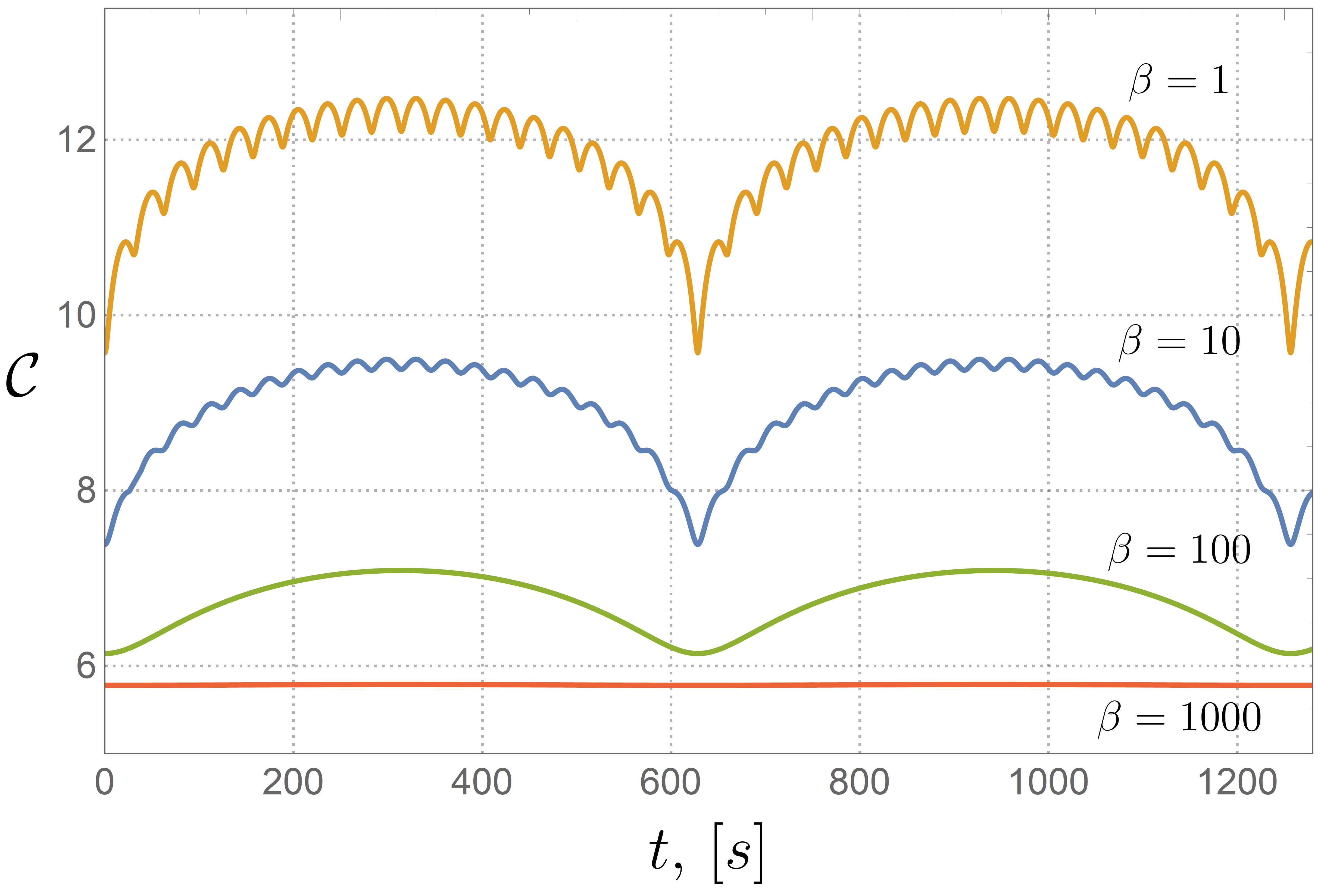
(a) Complexity $\mathcal{C}(t)$ at strong $B$.

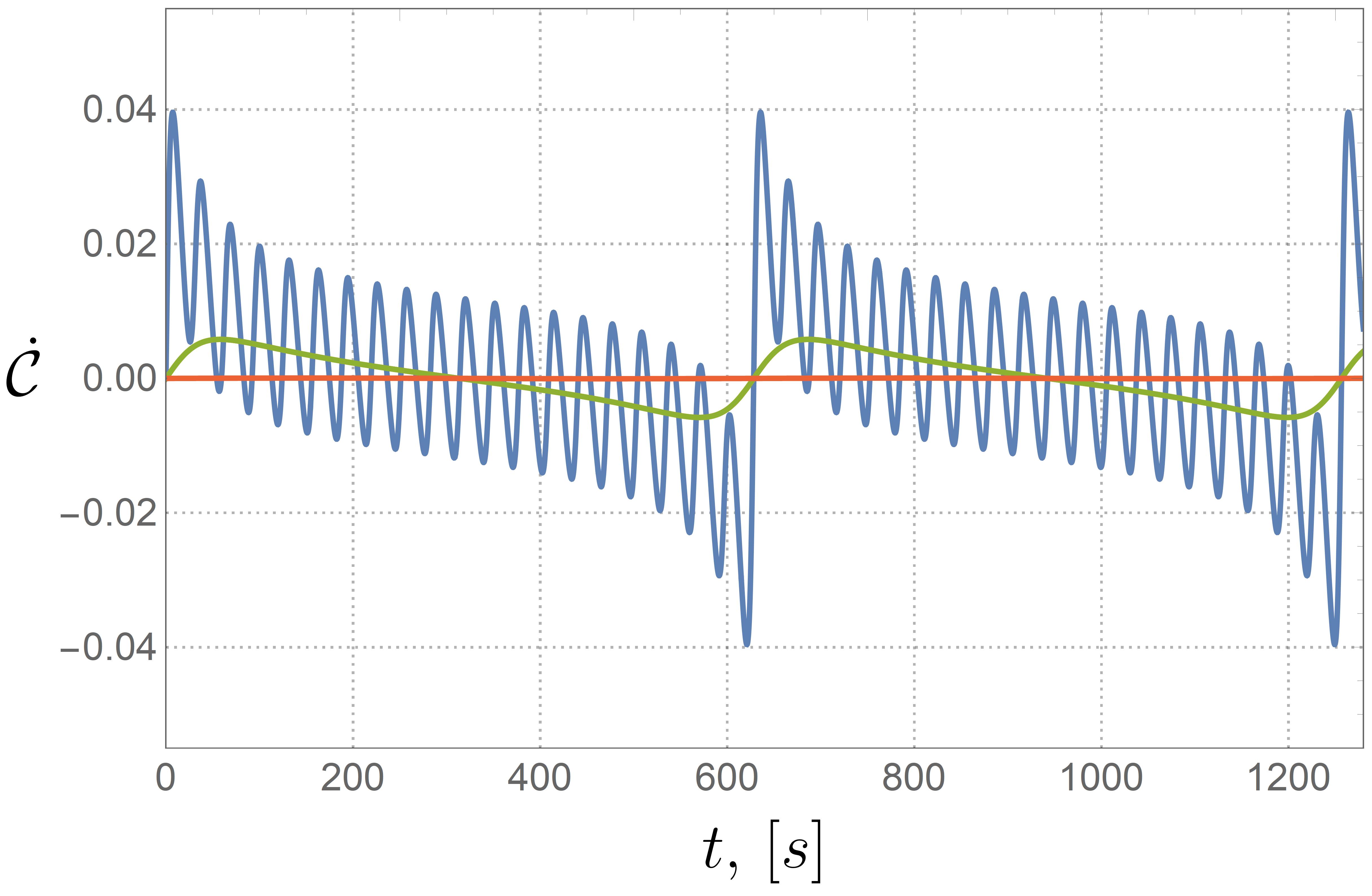
(b) Rate of complexity $\dot{\mathcal{C}}(t)$ at strong $B$.

Figure 1: Case I: $\omega_{1,2}<\omega_{R1,R2}=1$. (a) Complexity $\mathcal{C}(t)$ at strong external magnetic filed $\omega_{1}\gg\omega_{2}$. We choose: $\omega_{1}=0.1,\,\omega_{2}=0.005$ ($\omega_{c}=0.095,\,\omega_{0}=0.022$). (b) The corresponding rate of complexity $\dot{\mathcal{C}}(t)$ at strong magnetic field.

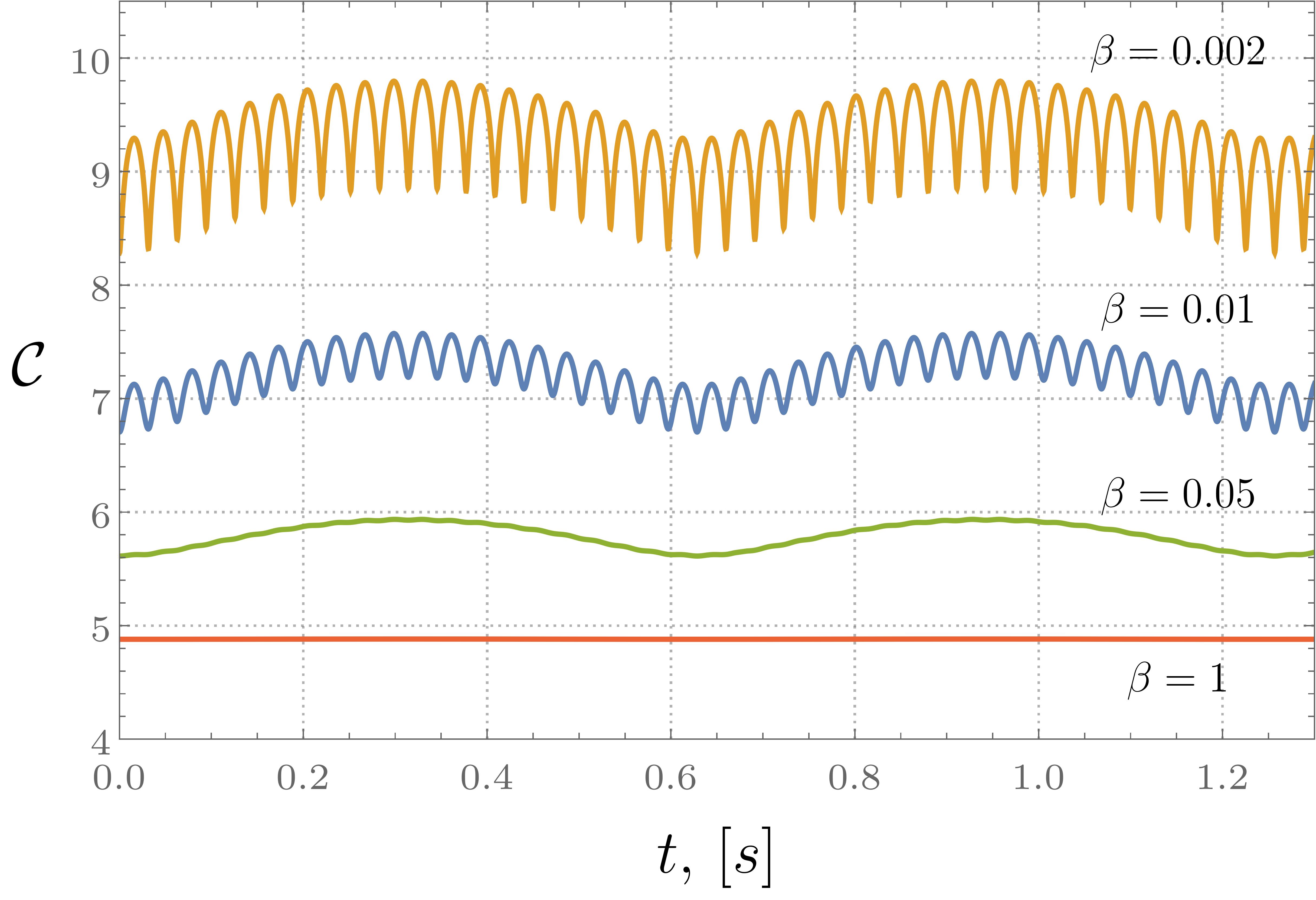
(a) Complexity $\mathcal{C}(t)$ at strong $B$.

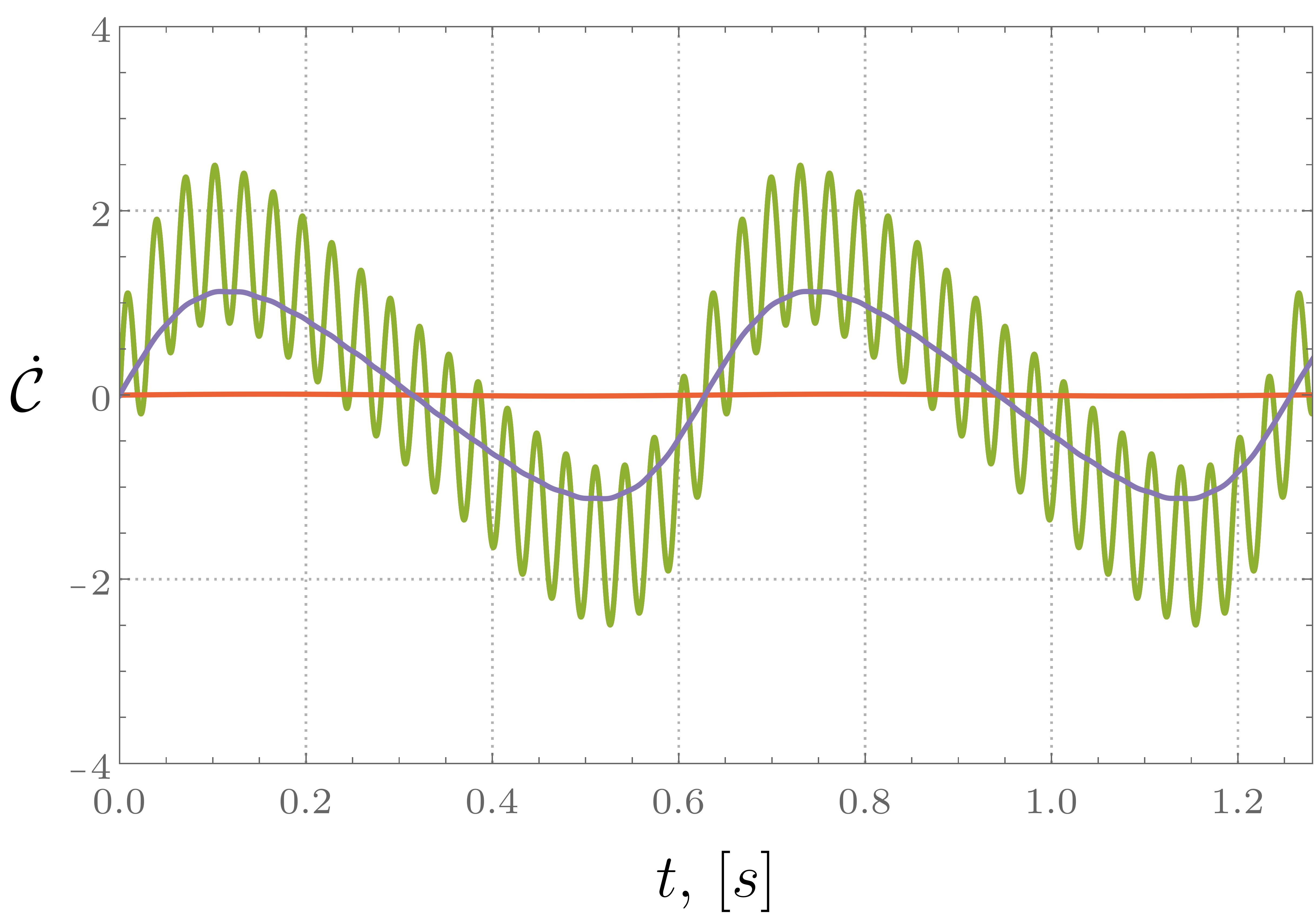
(b) Rate of complexity $\dot{\mathcal{C}}(t)$ at strong $B$.

Figure 2: Case II: $\omega_{1,2}>\omega_{R1,R2}=1$.(a) Complexity $\mathcal{C}(t)$ at strong external magnetic filed $\omega_{1}\gg\omega_{2}$. We choose: $\omega_{1}=100,\,\omega_{2}=5$ ($\omega_{c}=95,\,\omega_{0}=22$). (b) The corresponding rate of complexity $\dot{\mathcal{C}}(t)$ at strong magnetic field, where the green curve corresponds to $\beta=0.05$, purple: $\beta=0.1$, and red: $\beta=1$.

Weak magnetic field: In this case $\omega_{c}\ll\omega_{0}$, resulting in $\omega_{1}\approx\omega_{2}$. This situation is illustrated in Fig. 3 for $\omega_{1,2}<1$, where we observe a beating effect with a period

$$T\approx\frac{\pi}{\omega_{1}-\omega_{2}}.$$ (5.16)

This effect is more pronounced at high temperatures (shown by the orange and blue curves) and becomes less noticeable at low temperatures (depicted by the green and red curves). The complexity value corresponding to the red curve once again approaches the value given in Eq. (5.13). In the case of $\omega_{1,2}>1$ the behaviour of complexity is qualitative the same.

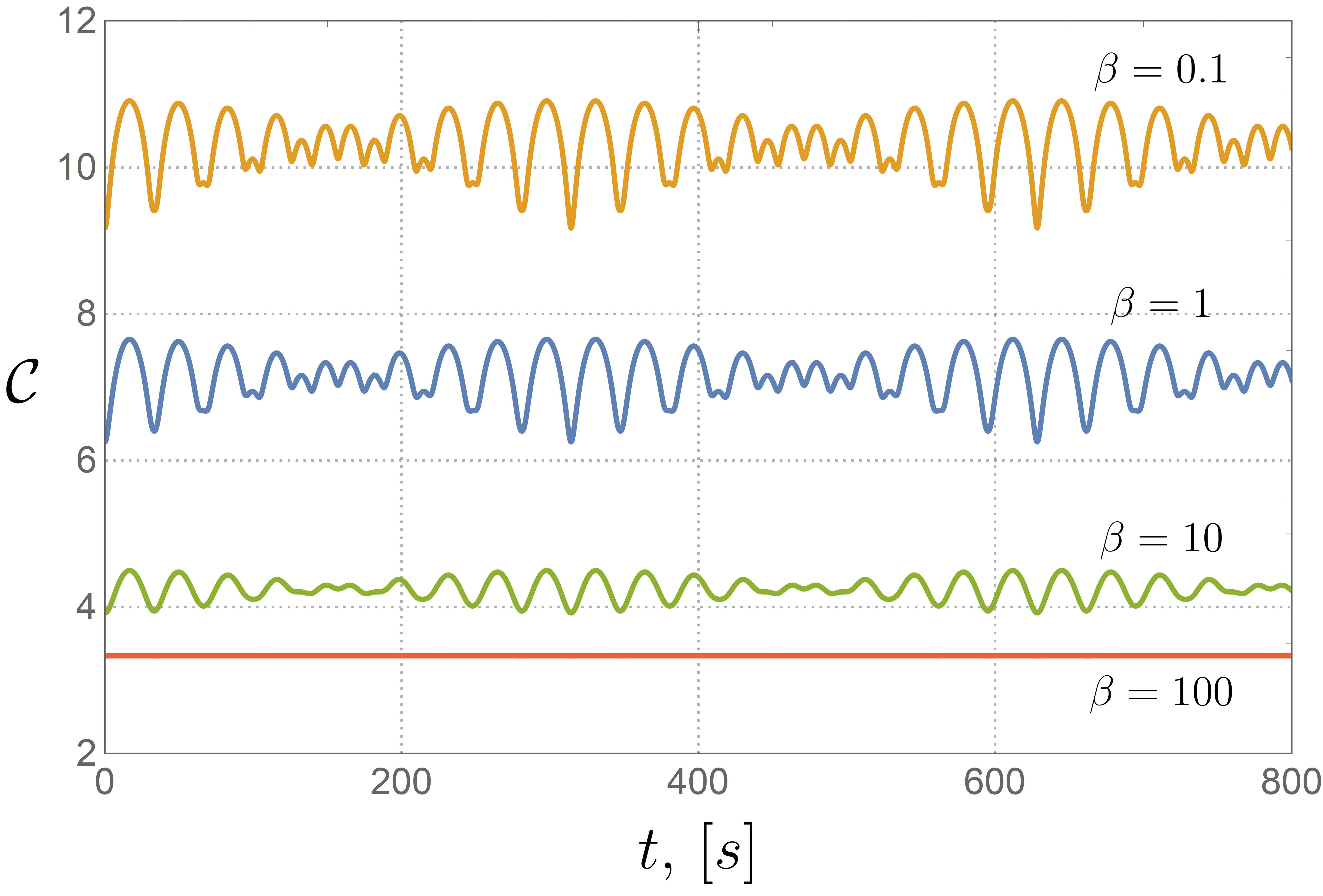
(a) Complexity $\mathcal{C}(t)$ at weak $B$.

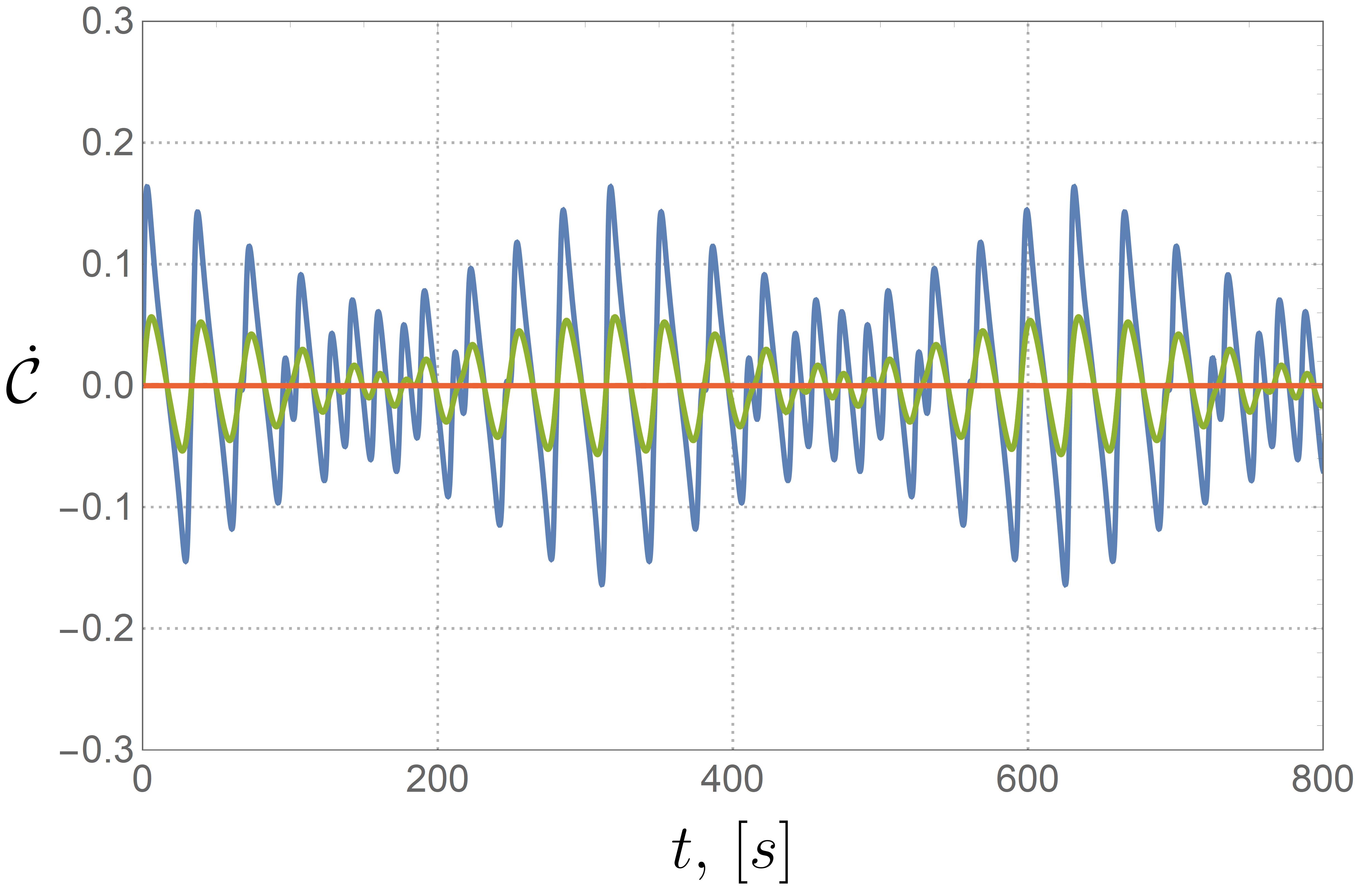
(b) Rate of complexity $\dot{\mathcal{C}}(t)$ at weak $B$.

Figure 3: Case I: $\omega_{1,2}<\omega_{R1,R2}=1$. (a) Complexity $\mathcal{C}(t)$ under weak external magnetic filed $\omega_{1}\approx\omega_{2}$. We choose: $\omega_{1}=0.1,\,\omega_{2}=0.09$ ($\omega_{c}=0.01,\,\omega_{0}=0.095$). (b) The corresponding rate of complexity $\dot{\mathcal{C}}(t)$ under weak magnetic field.

Zero magnetic field: Turning off the external magnetic field $\omega_{c}=0$ leads effectively to only one frequency $\omega_{1}=\omega_{2}=\omega_{0}$. The latter corresponds to two decoupled harmonic oscillators with equal frequencies. In this case, the time evolution of complexity is show on Fig. 4(a). The period of the oscillations is given by $T=\pi/\omega_{0}$.

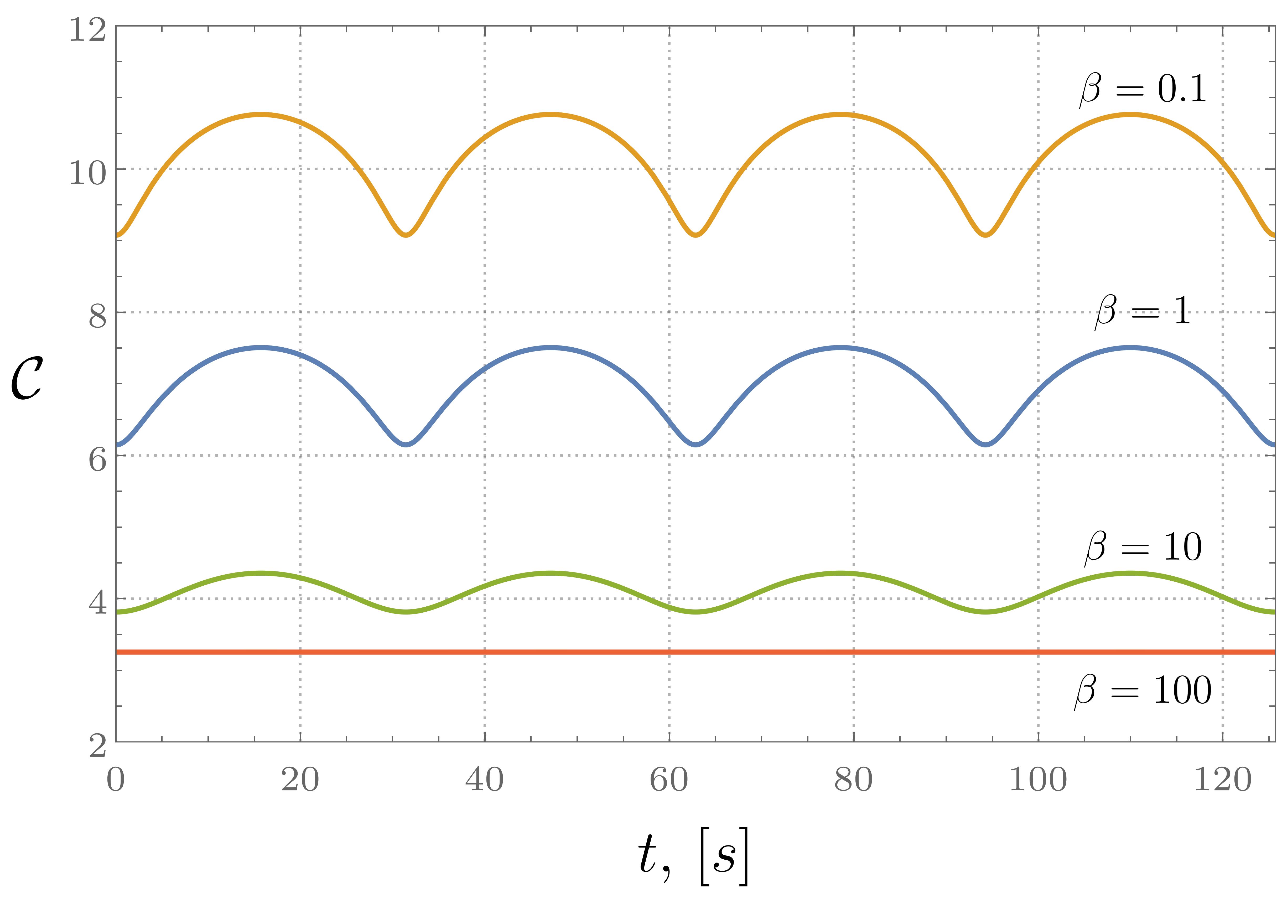
(a) Complexity $\mathcal{C}(t)$ at $B=0$.

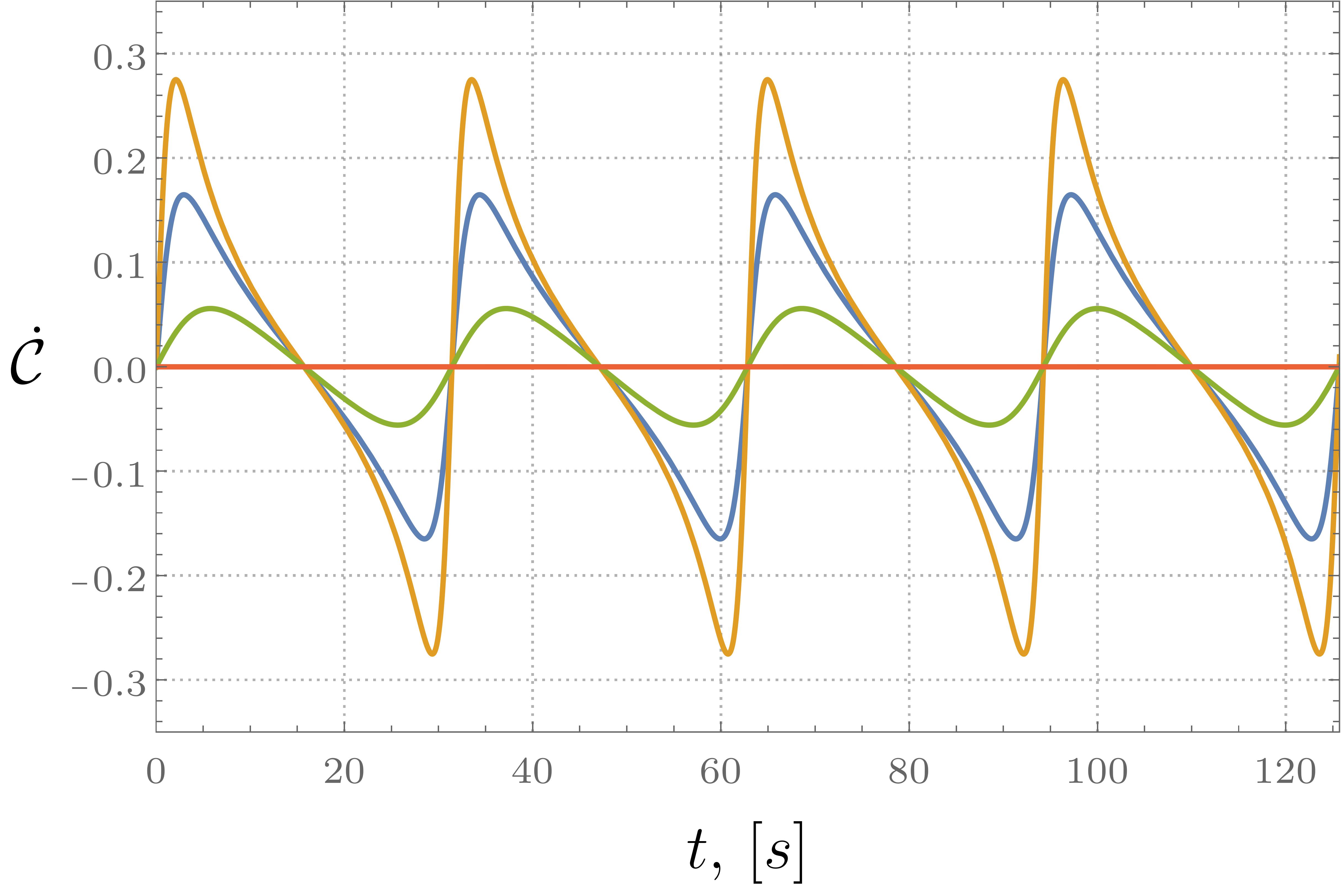
(b) Rate of complexity $\dot{\mathcal{C}}(t)$ at $B=0$.

Figure 4: For $B=0$ one has $\omega_{1}=\omega_{2}=\omega_{0}$. We choose $\omega_{0}=0.1$ for demonstration. (a) Complexity $\mathcal{C}(t)$ without magnetic field. (b) The rate of complexity $\dot{\mathcal{C}}(t)$ without magnetic field.

6 Rate of complexity and Lloyd’s bound

The internal energy of the TFD state follows directly from the partition function (3.2):

$$U=-\,\frac{\partial\ln Z}{\partial\beta}=\frac{\hbar}{2}\bigg{(}\omega_{1}\coth\frac{\beta\hbar\omega_{1}}{2}+\omega_{2}\coth\frac{\beta\hbar\omega_{2}}{2}\bigg{)}.$$ (6.1)

At very low temperatures $(\beta\to\infty)$ the internal energy reduces to the energy of the ground state (2.22):

$$\lim_{\beta\to\infty}U=\frac{\hbar}{2}(\omega_{1}+\omega_{2})=E_{0,0}.$$ (6.2)

At high temperatures $(\beta\hbar\omega_{i}\ll 1)$ the quantum effects become negligible and the internal energy behaves asymptotically as hyperbola

$$U\approx\frac{2}{\beta}.$$ (6.3)

Our goal is to compare the rate of complexity to the system’s internal energy, known as the Lloyd bound, which according to quantum information theory, is given by [47]:

$$|\dot{\mathcal{C}}|\leq\frac{2U}{\pi\hbar}.$$ (6.4)

The rate of complexity can be calculated from (5.8) yielding

$$\dot{\mathcal{C}}(t)=\frac{1}{4\mathcal{C}(t)}\sum_{s=1}^{8}\frac{\dot{e}_{s}}{e_{s}}\ln e_{s}.$$ (6.5)

In order to investigate whether the Lloyd bound is satisfied, we need to consider the maximum rate of complexity $|\mathcal{\dot{C}}|_{\rm{max}}$, which we define by the maximum absolute value of the derivative of complexity with respect to time. It has periodic nature as shown in Figs. 1(b)–4(b). We can demonstrate that the bound (6.4) is satisfied, as shown in Fig. 5. Notably, there are two distinct asymptotic behaviors. At very low temperatures ($\beta\to\infty$), the internal energy (green curve) approaches the ground state energy (6.2) (black dashed line), while the rate of complexity (blue curve) approaches zero (red dashed line).

$$\lim_{\beta\to\infty}U=E_{0,0},\quad\lim_{\beta\to\infty}\dot{\mathcal{C}}(t)=0.$$ (6.6)

At high temperatures ($\beta\to 0$), the internal energy diverges, while the maximum rate of complexity stabilizes at a finite value (depicted as a black dot):

$$\lim_{\beta\to 0}U=\infty,\quad\lim_{\beta\to 0}\dot{\mathcal{C}}(t)=\frac{1}{2\sqrt{2}}\sum_{i=1}^{2}\frac{\omega_{i}(\omega_{Ri}^{2}-\omega_{i}^{2})^{2}\sin 2\omega_{i}t}{(\omega_{Ri}^{2}+\omega_{i}^{2})^{2}-(\omega_{Ri}^{2}-\omega_{i}^{2})^{2}\cos^{2}\omega_{i}t}.$$ (6.7)

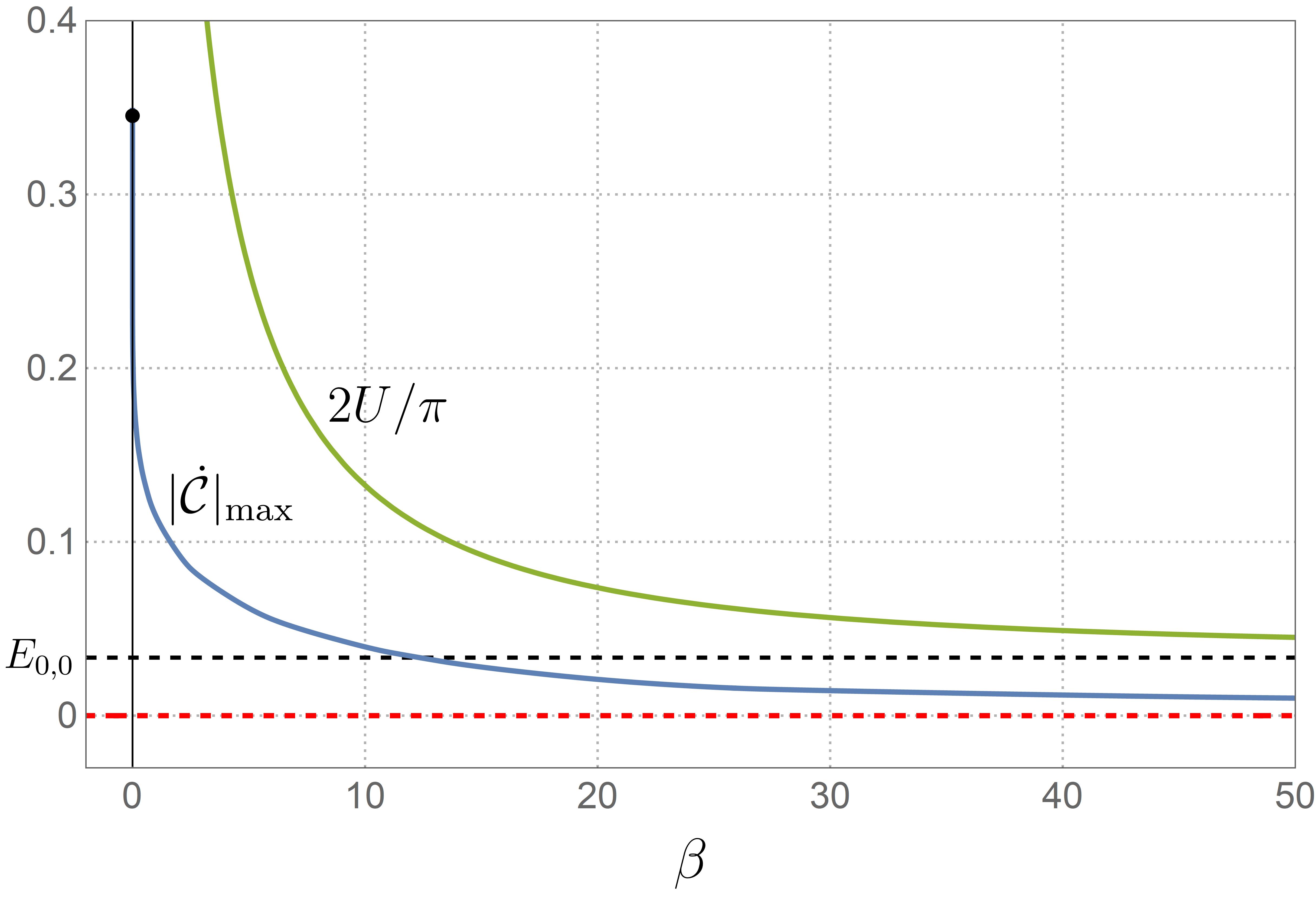
(a) $|\dot{\mathcal{C}}|_{\rm max}$ at strong $B$.

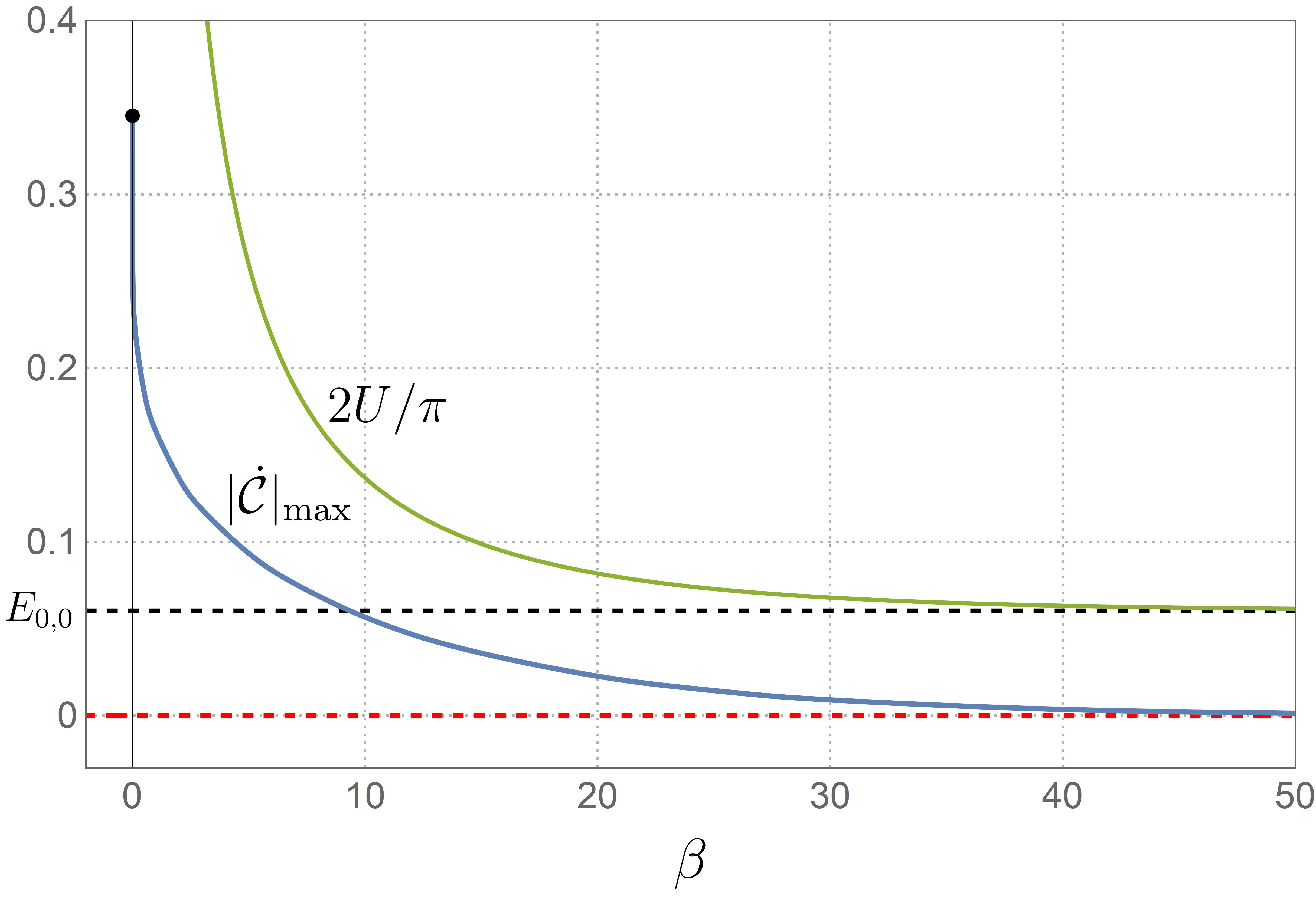
(b) $|\dot{\mathcal{C}}|_{\rm max}$ at weak $B$.

Figure 5: Maximum rate of complexity $|\dot{\mathcal{C}}|_{\rm max}$ (blue) and internal energy (green curve) as functions of $\beta$. (a) At strong magnetic field $\omega_{1}\gg\omega_{2}$. We choose: $\omega_{1}=0.1,\,\omega_{2}=0.005$. (b) At weak magnetic field $\omega_{1}\approx\omega_{2}$. We choose: $\omega_{1}=0.1,\,\omega_{2}=0.09$. In both cases we set $\omega_{R1}=\omega_{R2}=1$ and $\hbar=1$.

It is important to note that the ground state energies (6.2) differ between these two magnetic regimes. In any case, the ground state energy under a weak $B$ field is always higher than that in a strong $B$ field. Additionally, as $\beta$ increases, the internal energy and the maximum rate of complexity approach their corresponding asymptotes much faster in the weak $B$-field regime Fig. 5(b). For zero magnetic field $(\omega_{1}=\omega_{2}=\omega_{0})$ one has twice the internal energy of harmonic oscillator

$$U=\hbar\omega_{0}\coth\frac{\beta\hbar\omega_{0}}{2}.$$ (6.8)

In this case the Lloyd bound still holds.

7 Conclusion

In this work, we explored the Nielsen complexity of a thermofield double state for a harmonic oscillator subjected to an external magnetic field. This was accomplished using the covariance matrix method as outlined in [46], which is particularly well-suited for analyzing the evolution of Gaussian states. In general, Nielsen complexity defines the optimal paths connecting two such states. Building on these ideas, we obtained explicit results for the complexity and its rate, extensively studying the effects of temperature and the magnetic field.

We investigated the temperature dependence of complexity in two limiting cases: zero temperature and high temperature. In the zero temperature limit, the complexity saturates to a minimum positive value (5.13). In the high temperature limit, the complexity becomes unbounded from above (5.14). In all scenarios, an increase in temperature leads to a growth in the system’s complexity.

Regarding the effect of the magnetic field, we demonstrated that Nielsen complexity exhibits intriguing characteristics. For a strong magnetic field, complexity shows periodic behavior with a period primarily influenced by the lower frequency (5.15). For a weak magnetic field, complexity displays a beating effect (Fig. 3(a)) with a period defined in (5.16). Furthermore, we showed that in the absence of a magnetic field, the complexity reduces to that of two non-interacting harmonic oscillators.

Finally, we analyzed the Lloyd bound of the system, which relates the system’s internal energy to the maximum rate of complexity. We demonstrated that, regardless of temperature or magnetic field, the rate of complexity always adheres to this bound.

While this work focused on how an external magnetic field influences the complexity of a quantum oscillator, a similar study could be broadened to encompass more general systems. Such a comprehensive analysis may help clarify ambiguities in the definition of complexity across various contexts.

References

- [1] S. Ryu and T. Takayanagi, “Holographic derivation of entanglement entropy from AdS/CFT,” Phys. Rev. Lett. 96 (2006) 181602, arXiv:hep-th/0603001.
- [2] S. Ryu and T. Takayanagi, “Aspects of Holographic Entanglement Entropy,” JHEP 08 (2006) 045, arXiv:hep-th/0605073.
- [3] L. Susskind, “Entanglement is not enough,” Fortsch. Phys. 64 (2016) 49–71, arXiv:1411.0690 [hep-th].
- [4] L. Susskind, “Computational Complexity and Black Hole Horizons,” Fortsch. Phys. 64 (2016) 24–43, arXiv:1403.5695 [hep-th]. [Addendum: Fortsch.Phys. 64, 44–48 (2016)].
- [5] J. M. Maldacena, “Eternal black holes in anti-de Sitter,” JHEP 04 (2003) 021, arXiv:hep-th/0106112.
- [6] T. Hartman and J. Maldacena, “Time Evolution of Entanglement Entropy from Black Hole Interiors,” JHEP 05 (2013) 014, arXiv:1303.1080 [hep-th].
- [7] A. R. Brown, D. A. Roberts, L. Susskind, B. Swingle, and Y. Zhao, “Holographic Complexity Equals Bulk Action?,” Phys. Rev. Lett. 116 no. 19, (2016) 191301, arXiv:1509.07876 [hep-th].
- [8] J. Couch, W. Fischler, and P. H. Nguyen, “Noether charge, black hole volume, and complexity,” JHEP 03 (2017) 119, arXiv:1610.02038 [hep-th].
- [9] A. Belin, R. C. Myers, S.-M. Ruan, G. Sárosi, and A. J. Speranza, “Does Complexity Equal Anything?,” Phys. Rev. Lett. 128 no. 8, (2022) 081602, arXiv:2111.02429 [hep-th].
- [10] A. Belin, R. C. Myers, S.-M. Ruan, G. Sárosi, and A. J. Speranza, “Complexity equals anything II,” JHEP 01 (2023) 154, arXiv:2210.09647 [hep-th].
- [11] E. Jørstad, R. C. Myers, and S.-M. Ruan, “Complexity=anything: singularity probes,” JHEP 07 (2023) 223, arXiv:2304.05453 [hep-th].
- [12] R. C. Myers and S.-M. Ruan, “Complexity Equals (Almost) Anything,” 3, 2024. arXiv:2403.17475 [hep-th].
- [13] S. Arora and B. Barak, Computational Complexity: A Modern Approach. Cambridge University Press, 2009. https://books.google.de/books?id=8Wjqvsoo48MC.
- [14] C. Moore and S. Mertens, The Nature of Computation. OUP Oxford, 2011. https://books.google.de/books?id=jnGKbpMV8xoC.
- [15] M. A. Nielsen, “A geometric approach to quantum circuit lower bounds,” Quant. Inf. Comput. 6 no. 3, (2006) 213–262, arXiv:quant-ph/0502070.
- [16] M. Nielsen and I. Chuang, Quantum Computation and Quantum Information: 10th Anniversary Edition. Cambridge University Press, 2010. https://books.google.de/books?id=-s4DEy7o-a0C.
- [17] M. R. Dowling and M. A. Nielsen, “The geometry of quantum computation,” Quant. Inf. Comput. 8 no. 10, (2008) 0861–0899, arXiv:quant-ph/0701004.
- [18] M. A. Nielsen, M. R. Dowling, M. Gu, and A. C. Doherty, “Quantum Computation as Geometry,” Science 311 no. 5764, (2006) 1133–1135, arXiv:quant-ph/0603161.
- [19] T. Cormen, C. Leiserson, R. Rivest, and C. Stein, Introduction To Algorithms. Mit Electrical Engineering and Computer Science. MIT Press, 2001. https://books.google.de/books?id=NLngYyWFl_YC.
- [20] S. Chapman, J. Eisert, L. Hackl, M. P. Heller, R. Jefferson, H. Marrochio, and R. C. Myers, “Complexity and entanglement for thermofield double states,” SciPost Phys. 6 no. 3, (2019) 034, arXiv:1810.05151 [hep-th].
- [21] M. Ghasemi, A. Naseh, and R. Pirmoradian, “Odd entanglement entropy and logarithmic negativity for thermofield double states,” JHEP 10 (2021) 128, arXiv:2106.15451 [hep-th].
- [22] M. Doroudiani, A. Naseh, and R. Pirmoradian, “Complexity for Charged Thermofield Double States,” JHEP 01 (2020) 120, arXiv:1910.08806 [hep-th].
- [23] F. Khorasani, R. Pirmoradian, and M. R. Tanhayi, “Position dependence of Nielsen complexity for the thermofield double state,” Phys. Lett. B 851 (2024) 138585, arXiv:2308.15836 [quant-ph].
- [24] S. Chapman, M. P. Heller, H. Marrochio, and F. Pastawski, “Toward a Definition of Complexity for Quantum Field Theory States,” Phys. Rev. Lett. 120 no. 12, (2018) 121602, arXiv:1707.08582 [hep-th].
- [25] A. Bhattacharyya, A. Shekar, and A. Sinha, “Circuit complexity in interacting QFTs and RG flows,” JHEP 10 (2018) 140, arXiv:1808.03105 [hep-th].
- [26] T. Ali, A. Bhattacharyya, S. Shajidul Haque, E. H. Kim, and N. Moynihan, “Time Evolution of Complexity: A Critique of Three Methods,” JHEP 04 (2019) 087, arXiv:1810.02734 [hep-th].
- [27] R. Jefferson and R. C. Myers, “Circuit complexity in quantum field theory,” JHEP 10 (2017) 107, arXiv:1707.08570 [hep-th].
- [28] B. K. Bagchi, Supersymmetry in quantum and classical mechanics. 2001.
- [29] E. I. Jafarov and J. Van der Jeugt, “The oscillator model for the Lie superalgebra sh(2|2) and Charlier polynomials,” J. Math. Phys. 54 (2013) 103506, arXiv:1304.3295 [math-ph].
- [30] B. W. Fatyga, V. A. Kostelecky, M. M. Nieto, and D. R. Truax, “Supercoherent states,” Phys. Rev. D 43 (1991) 1403–1412.
- [31] B. P. Mandal and S. K. Rai, “Noncommutative Dirac oscillator in an external magnetic field,” Phys. Lett. A 376 (2012) 2467–2470, arXiv:1203.2714 [hep-th].
- [32] J. Jing and J.-F. Chen, “Non-commutative harmonic oscillator in magnetic field and continuous limit,” Eur. Phys. J. C 60 (2009) 669–674.
- [33] J. Ben Geloun, S. Gangopadhyay, and F. G. Scholtz, “Harmonic oscillator in a background magnetic field in noncommutative quantum phase-space,” EPL 86 no. 5, (2009) 51001, arXiv:0901.3412 [hep-th].
- [34] M. Heddar, M. Falek, M. Moumni, and B. C. Lütfüoğlu, “Pauli oscillator in noncommutative space,” Mod. Phys. Lett. A 36 no. 40, (2021) 2150280, arXiv:2110.00723 [hep-th].
- [35] A. Boumali, F. Serdouk, and S. Dilmi, “Superstatistical properties of the one-dimensional Dirac oscillator,” Physica A 553 (2020) 124207.
- [36] M. Falek, M. Merad, and T. Birkandan, “Duffin–Kemmer–Petiau oscillator with Snyder-de Sitter algebra,” J. Math. Phys. 58 no. 2, (2017) 023501.
- [37] S. M. Nagiyev and R. M. Mir-Kasimov, “Relativistic linear oscillator under the action of a constant external force. Transition amplitudes and the Green’s function,” Theor. Math. Phys. 214 no. 1, (2023) 72–88.
- [38] R. P. Martinez-y Romero, H. N. Nunez-Yepez, and A. L. Salas-Brito, “Relativistic quantum mechanics of a Dirac oscillator,” Eur. J. Phys. 16 (1995) 135–141, arXiv:quant-ph/9908069.
- [39] P. D. Mannheim and A. Davidson, “Dirac quantization of the Pais-Uhlenbeck fourth order oscillator,” Phys. Rev. A 71 (2005) 042110, arXiv:hep-th/0408104.
- [40] I. Masterov, “An alternative Hamiltonian formulation for the Pais–Uhlenbeck oscillator,” Nucl. Phys. B 902 (2016) 95–114, arXiv:1505.02583 [hep-th].
- [41] H. Dimov, S. Mladenov, R. C. Rashkov, and T. Vetsov, “Entanglement of higher-derivative oscillators in holographic systems,” Nucl. Phys. B 918 (2017) 317–336, arXiv:1607.07807 [hep-th].
- [42] S. Pramanik and S. Ghosh, “Taming the Ghost in Pais-Uhlenbeck Oscillator,” Mod. Phys. Lett. A 28 (2013) 1350038, arXiv:1205.3333 [math-ph].
- [43] H. Bouguerne, B. Hamil, B. C. Lütfüoğlu, and M. Merad, “Dunkl-Pauli Equation in the Presence of a Magnetic Field,” arXiv:2309.14081 [quant-ph].
- [44] B. Hamil and B. C. Lütfüoğlu, “Thermal properties of relativistic Dunkl oscillators,” Eur. Phys. J. Plus 137 no. 7, (2022) 812, arXiv:2202.02871 [quant-ph].
- [45] A. Ballesteros, A. Najafizade, H. Panahi, H. Hassanabadi, and S.-H. Dong, “The Dunkl oscillator on a space of nonconstant curvature: An exactly solvable quantum model with reflections,” Annals Phys. 460 (2024) 169543, arXiv:2212.13575 [quant-ph].
- [46] S. Chapman, J. Eisert, L. Hackl, M. P. Heller, R. Jefferson, H. Marrochio, and R. Myers, “Complexity and entanglement for thermofield double states,” SciPost physics 6 no. 3, (2019) 034.
- [47] S. Lloyd, “Ultimate physical limits to computation,” Nature 406 no. 6799, (2000) 1047–1054.