IOVS4NeRF: Incremental Optimal View Selection
for Large-Scale NeRFs

Abstract

Urban-level three-dimensional reconstruction for modern applications demands high rendering fidelity while minimizing computational costs. The advent of Neural Radiance Fields (NeRF) has enhanced 3D reconstruction, yet it exhibits artifacts under multiple viewpoints. In this paper, we propose a new NeRF framework method to address these issues. Our method uses image content and pose data to iteratively plan the next best view. A crucial aspect of this method involves uncertainty estimation, guiding the selection of views with maximum information gain from a candidate set. This iterative process enhances rendering quality over time. Simultaneously, we introduce the Vonoroi diagram and threshold sampling together with flight classifier to boost the efficiency, while keep the original NeRF network intact. It can serve as a plug-in tool to assist in better rendering, outperforming baselines and similar prior works.

I Introduction

The essence of image-based 3D reconstruction is to infer the geometry and structure of objects and scenes from single or multiple 2D images. This longstanding challenge with broad implications is fundamental to many applications from scene understanding to object recognition, including medical diagnosis, robot navigation, 3D modeling and industrial control. The task of 3D reconstruction has indeed matured, as evidenced by commercial products such as Agisoft and Pix4D, which are capable of delivering high-fidelity, large-scale 3D models.

There’s a growing trend to harness deep learning algorithms inspired by animal vision[1, 2]. Exploring the fusion of 3D reconstruction and deep learning has revealed new possibilities, yet significant challenges persist.For instance, Point clouds[3, 4], consists of points with 3D coordinates, potentially incorporating color and reflectance intensity information. However, it lacks surface connectivity and the reconstructed surfaces appearing less smooth.

In contrast to previous methods, Neural Radiance Fields (NeRF)[5] utilizes neural networks to represent the radiance field in a scene. NeRF employs a simple multi-layer perceptron (MLP) network, and volumetric rendering for novel view synthesis and image reconstruction. It utilizes a straightforward five-dimensional input comprising three-dimensional spatial coordinates ($x,y,z$) and two-dimensional ray directions ($\theta,\phi$) to ultimately produce color and voxel density for images. Despite its efficacy, NeRF’s implicit neural network results in resource-intensive computations[6] and demands substantial pose information for training[7, 8], leading to inefficiencies in large scenes.

Figure 1: Novel view synthesis comparison. We propose a new NeRF framework, and the comparision on the ArtSci dataset across four different model strategies, revealing that our method outperforms others in terms of both processing time and reconstruction efficacy.

View Planning. Our view selection in this article is based on view planning[9]. It involves determining the optimal angles, positions, and camera or sensor settings for capturing relevant information. Various visual tasks necessitate distinct viewpoint planning algorithms, broadly categorized into search-based and synthesis-based methods. Search-based methods involve sampling numerous candidate views and selecting specific views under certain constraints, whereas synthesis methods significantly reduce computational costs but lack sufficient reliability and accuracy.

The Next-Best view (NBV) problem[10] is a specific subfield of view planning. In NBV, algorithms assess information gain or target visibility from different viewpoints, selecting the most valuable or informative view to advance the task. Requirements for search-based viewpoint planning include: (1) sampling a specific number of candidate views in the view space (2) simulating visual information for each candidate view and estimating the information gain (3) selecting the optimal viewpoint or a set of viewpoints.

Figure 2: IOVS4NeRF is a flexible framework that actively expands the existing training set with newly captured samples based on computed uncertainties of candidate views. IOVS4NeRF incorporates rendering uncertainty and the positional uncertainty of scene uncertainty at unobserved novel views. By selecting the view that brings the most information gain, the quality of novel view synthesis can be improved with minimal additional resources.

Information Gain. Our method quantifies selection criteria through information gain. Originally, information entropy is utilized to describe the uncertainty and randomness of information, representing the complexity of a random variable. Information gain is defined as the amount of information a feature can bring to a classification system; higher information gain indicates greater feature importance.

In the NeRF-NBV problem[11], uncertainty quantification is often expressed as a representation of uncertainty. Existing research frequently employs uncertainty quantification results as the expression of information gain. In deep learning, uncertainty estimation methods mainly include Bayesian estimation (as seen in S-Nerf[12]), MC Dropout[13], and model ensembles[14]. Model ensembles reduce the bias and variance of a single model by combining predictions from multiple models. Expanding on this, given the context of drone flight, we integrate rendering uncertainty and position uncertainty as novel standard reference. We treat both with equal importance to pinpoint the next best view that maximizes information gain.

IOVS4NeRF. In our NeRF method, tailored processing methods are applied based on distinct flight trajectories. Initially, an adaptive classifier is trained to discern whether a given aerial trajectory, captured through images, is planar or non-planar. Despite the majority of drone photography trajectories could be seen planar[15, 16], we enhance the classifier’s generalization capability. For planar trajectories, we compress and confine position uncertainty within Voronoi information radiation field. Conversely, for non-planar trajectories, a Voronoi clustering algorithm is employed to derive uncertainty from the distances between different viewpoints and a central point.

Given the challenges posed by the lengthy training time and insufficient preservation of detailed information inherent in position encoding and MLP implicit networks, we use Instant-NGP[17] as a tool to assist us better render our scene. In the context of volume rendering, it has been demonstrated[18, 6]that NeRF struggles to generalize effectively from a limited number of input views. When the scene observations are incomplete, the original NeRF framework tends to collapse to trivial solutions by predicting zero volume density for unobserved regions. To address this, we model the radiance color at each position in the scene as a beta distribution, aligning with its mathematical properties between 0 and 1. This modeling approach not only simplifies computations but also provides a better fit for large scenes, adding a crucial refinement to the overall framework method, as mentioned in Figure 1.

In summary, our contributions are as follows.

• We propose IOVS4NeRF, a novel NeRF approach for efficient 3D scene reconstruction in large-scale environments. Using a lightweight network architecture and enhanced volumetric rendering techniques, our method achieves significant improvements in both training and rendering efficiency.

• We use rendering uncertainty together with position uncertainty as the mixed criterion proxy for the total information gain of the underlying 3D geometry, and we present an uncertainty guided policy using NeRF representation for next-best-view selection.

• Our strategy, while maintaining reconstruction effectiveness, significantly reduces the time required for 3D reconstruction. Extensive experiments on real-world datasets have been performed to show the efficiency of the proposed method.

II Related Work

Traditional Real Scene Reconstruction. Traditional 3D modeling data acquisition mainly includes manual modeling and oblique photogrammetry. Due to the labor-intensive nature and low efficiency of manual modeling tools such as 3DSMax and Sketch Up, oblique photogrammetry with drones equipped with five-lens cameras capturing image data from multiple angles to obtain complete and accurate texture data and position information has a slight advantage. However, its reconstruction still follows three steps. The first is Structure from Motion (SfM[19]), which analyzes feature points in image sequences, utilizes bundle adjustment parameters to obtain 3D structure and camera trajectories. This is followed by Multi-View Stereo(MVS[20]), which estimates depth maps for each viewpoint to generate a single-viewpoint cloud. Finally, surface reconstruction merges different viewpoint clouds and conducts surface reconstruction[21].

With the development of deep learning, scholars have integrated this method into 3D modeling. DeepVO[22] uses deep recursive CNN to directly infer poses from a series of RGB images, bypassing traditional visual odometry modules. BA-Net[23] incorporates the Bundle Adjustment (BA) optimization algorithm as a layer in a neural network. This is done to train a more efficient set of basis functions, simplifying the backend optimization process during reconstruction.

Uncertainty Estimation. In computer vision, there’s a growing recognition of the crucial role uncertainty estimation plays. It not only enhances the interpretability of neural network outputs but also mitigates the risks of critical errors in important tasks. This trend reflects a heightened focus on the reliability of deep learning models. A detailed analysis of uncertainty in predictions offers a more thorough understanding of model behavior in complex real-world scenarios, paving the way for more reliable solutions.

This development primarily comprises two components: Bayesian Neural Networks (BNN)[24] and Dropout Variational Inference[25]. BNN treats the weights of neural networks as parameters of probability distributions, introducing prior and posterior distributions to infer the uncertainty in model outputs. Dropout Variational Inference, on the other hand, utilizes dropout layers for multiple inferences, estimating uncertainty by sampling different subnetworks.

Furthermore, research explores the application of uncertainty estimation in the domain of novel view synthesis. NeRF-W[26] introduces uncertainty to model transient objects in a scene, focusing on differences between images rather than inherent noise in training data, as observed in ActiveNeRF[27]. Tri-MipRF[28] approximates cones with a multivariate Gaussian, constructing inscribed spheres for sample points. It projects these spheres orthogonally onto three planes, obtaining circular projections.

NoPe-NeRF[29] utilizes only color and depth uncertainty without considering camera pose. The novel depth loss proposed in this paper learns scale and shift parameters for inter-frame depth, equivalent to maintaining geometrically consistent scenes during learning. However, these complex training and rendering processes can be daunting. Thus, we propose rendering uncertainty, combining position uncertainty. Additionally, in the domain of unmanned aerial vehicles, we innovatively incorporate Voronoi diagram[30, 31] to quantify position uncertainty, significantly reducing training and rendering time.

Fast Training and Rendering in Large Scenes. City-level radiance fields, exemplified by approaches like CityNeRF[32], Mega-NeRF[33], and Grid-NeRF[34], represent significant advancements tailored specifically for urban environments. Urban Radiance Fields effectively leverage RGB images and LiDAR scan data for 3D reconstruction and novel view synthesis. Subsequent papers build upon this foundation, incorporating Deformable Neural Mesh Primitives (DNMP[35]) as a novel carrier. Initially, DNMP is generated from point clouds, and through rasterization, ray-DNMP intersection points are computed. Feature interpolation is employed, coupled with view-dependent embedding, to determine radiance values and opacity .

CityNeRF employs a progressive learning strategy, activating high-frequency channels in position encoding to preserve intricate details during training. On the other hand, BlockNeRF[36] trains individual blocks within scene subdivisions, enabling fine-tuning block by block. Mega-NeRF utilizes NeRF++[37] for vast, unbounded scenes and enhances background expressiveness. It also incorporates the appearance embedding method from NeRF-W to balance varying lighting conditions across different images within the same scene.

Grid-guided Neural Radiance Fields[34] propose a two-branch model, consisting of a pretraining Grid branch stage and a Joint Learning Grid-and-NERF branches stage. During the joint learning stage, grid branch loss and nerf branch loss are jointly optimized. The sampling points are positioned closer to object surfaces, resulting in impressive outcomes. These methods collectively propel advancements in understanding and rendering urban-level scenes, fostering applications within urban environments.

Figure 3: Overview of our framework. Our pipeline consists of three parts: I. Based on the 5D information of the images, we input them into NeRF for training. We define the color at a certain position as a beta distribution and quantitatively obtain the mean and variance of color from the MLP, generating our rendering uncertainty. II. We extract the positional information of the images from the training set and input them into a classifier to determine their respective Voronoi positional uncertainty, resulting in hybrid uncertainty. III. Based on the hybrid information uncertainty, we select the images with the maximum gain from the candidate set and add them to the training set, iterating continuously.

III Background

In this section, we provide a brief overview of the NeRF framework and more details of this algorithm can be found in [5].

NeRF represents a scene as a continuous function $F_{\theta}$ that outputs both the emitted radiance value and volume density. Specifically, given a 3D position $\mathbf{x}=(x,y,z)$ in the scene and a viewing direction vector $\mathbf{d}=(\theta,\phi)$, a multi-layer perceptron model is used to generate the corresponding volume density $\sigma$ and color $\mathbf{c}=(r,g,b)$ as follows:

$$[\sigma,f]=\text{MLP}_{\theta_{1}}(\gamma_{x}(\mathbf{x})),$$ (1)

$$c=\text{MLP}_{\theta_{2}}(f,\gamma_{d}(\mathbf{d})),$$ (2)

, where $\gamma_{x}(\cdot)$ and $\gamma_{d}(\cdot)$ are the positional encoding functions, and $f$ represents the intermediate feature that is independent of the viewing direction $\mathbf{d}$. An interesting observation is that the radiance color is influenced solely by its own 3D coordinates and the viewing direction, rendering it independent of other locations.

To enable free novel synthesis, NeRF utilizes volume rendering to determine the color of rays passing through the scene. Given a camera ray $\mathbf{r}(t)=\mathbf{o}+t\mathbf{d}$ with the camera center $\mathbf{o}\in\mathbb{R}^{3}$ passing through a specific pixel on the image plane, the color of the pixel can be expressed as:

$$C(\mathbf{r})=\int_{t_{n}}^{t_{f}}T(t)\sigma(\mathbf{r}(t))c(\mathbf{r}(t),\mathbf{d})dt,$$ (3)

,where $T(t)=\exp\left(-\int_{t_{n}}^{t}\sigma(\mathbf{r}(s))ds\right)$ denotes the accumulated transmittance, and $t_{n}$ and $t_{f}$ are the near and far bounds in the scene. To simplify the rendering process, NeRF approximates the integral using stratified sampling and represents it as a linear combination of sampled points:

$$\hat{C}(\mathbf{r}) =\sum_{i=1}^{N_{s}}\alpha_{i}c(\mathbf{r}(t_{i}))$$ (4)

$$\alpha_{i} =\exp\left(-\sum_{j=1}^{i-1}\sigma_{j}\delta_{j}\right)\left(1-\exp(-\sigma_{i}\delta_{i})\right)$$

,where $\delta_{i}=t_{i+1}-t_{i}$ is the distance between adjacent samples, and $N_{s}$ denotes the number of samples.Based on this approach, NeRF optimizes the continuous function $F_{\theta}$ by minimizing the squared reconstruction errors between the ground truth RGB images $\{I_{i=1}^{N}\}$ and the rendered pixel colors.

To enhance sampling efficiency, NeRF simultaneously optimizes two parallel networks, referred to as the coarse and fine models. The sampling strategy for the fine model is refined based on the results of the coarse model, with samples being biased towards more relevant regions. Overall, the optimization loss is parameterized as follows:

$$\sum_{i}\left\|C(\mathbf{r_{i}})-\hat{C}^{c}(\mathbf{r_{i}})\right\|_{2}^{2}+\left\|C(\mathbf{r_{i}})-\hat{C}^{f}(\mathbf{r_{i}})\right\|_{2}^{2},$$ (5)

, where $\mathbf{r_{i}}$ is a sampled ray, and $C(\mathbf{r_{i}}),\hat{C}^{c}(\mathbf{r_{i}}),\hat{C}^{f}(\mathbf{r_{i}})$ correspond to the ground truth, coarse model prediction, and fine model prediction respectively.

IV IOVS4NeRF

In this paper, we focus on optimal view selection for large-scale NeRFs. In this section, we present the IOVS4NeRF framework in section. IV-A followed by detailed descriptions of the proposed hybrid-uncertainty estimation (section. IV-B) and implementation (section. IV-C).

IV-A Framework

As shown in Fig. 3, the IOVS4NeRF framework consists of 3 steps. First, the random views are used to train for initialization. Then in every expansion round, we compute the uncertainties of each unused candidate view added to the one with the highest score into the training set until the quality of the synthesized novel view meets the requirement.

1) Initialization. As shown in Fig. 2, we randomly select a fixed proportion of images (we experimentally recommend 15%) from the input dataset to perform NeRF training for initialization.

2) Uncertainty estimation. Note that the IOVS4NeRF selects the best view based on the information gain metric, named hybrid-uncertainty, with two main terms: 1) rendering uncertainty and 2) positional uncertainty:

For rendering uncertainty, we input 5D coordinates (x,d) of the remaining photo set into a modified NeRF network with threshold sampling, which then outputs both color c and volume density variance. Subsequently, we calculate the rendering uncertainty of the image by integrating both c and variance into a beta distribution.

For positional uncertainty, we input 3D coordinates x of the remaining photo set, and a classifier determines whether the trajectory is planar or non-planar. We then estimate the position information using Voronoi diagrams to obtain the positional uncertainty.

Then, we normalize and sum the two uncertainty to calculate the hybrid uncertainty, as shown in the following formula:

$${\psi^{2}}(I)=Norm(\sigma_{pos}^{2}(I))+Norm(\sigma_{rgb}^{2}(I))$$ (6)

, I means the ground truth RGB images and the function $Norm(\cdot)$ representing normalization. The formula $\sigma_{pos}^{2}(I)$ and $\sigma_{rgb}^{2}(I)$ can been seen at Eq. (17) and Eq. (7).

We select the image with the highest hybrid uncertainty and continually add it to the training set. This process is repeated until a specific reconstruction effect is achieved or a preset limit on the number of selected images is reached.

We partition the hybrid uncertainty into rendering uncertainty and position uncertainty. Kendall and Gal[38] identified two types of uncertainty relevant to computer vision—aleatoric uncertainty and epistemic uncertainty, and our uncertainty belongs to the latter type, which can be reduced with more data.

$$\sigma_{rgb}^{2}(I)=\sum\limits_{i=1}^{{N_{r}}}{\frac{{||C({{\bf{r}}_{i}})-\bar{C}({{\bf{r}}_{i}})||_{2}^{2}}}{{2{{\bar{\beta}}^{2}}({{\bf{r}}_{i}})}}+\frac{{\log{{\bar{\beta}}^{2}}({{\bf{r}}_{i}})}}{2}}$$ (7)

, where $N_{r}$ means the total number of the rays in photo I.

Figure 4: For planar flight trajectories, we use Voronoi information radiation fields, with the top-level global planner employing a generalized Voronoi diagram to create and update a list of Voronoi nodes. The bottom-level local planner selects the largest node from the list based on the potential field formed by the weighted centroids, uploading it to the top level planner for further filtering.

IV-B Hybrid-Uncertainty Estimation

$\bullet$ Rendering Uncertainty.

Focused on scenarios with limited training data, if the scene observation is incomplete, the original NeRF framework often collapses into fragmented results by predicting zero volume density for unobserved regions. As a remedy, we propose modeling the color rgb value at each position in the scene as a beta distribution[39, 40] rather than a single value. The predicted variance can reflect the uncertainty at a particular position. This approach allows the model to provide larger variances in unobserved regions, thus maintaining greater information gain for completing renderings and reducing the overall model’s epistemic uncertainty.

Moreover, by constraining color values between 0 and 1, in line with the mathematical characteristics of the beta distribution, its conjugate prior inherently includes the partition function in the Bayesian formula, thereby avoiding complex global integrals in Bayesian inference. Thus, it can be quantitatively calculated and scaled in large-scale scenes.

Specifically, we define the color at a certain position as a beta distribution with parameters representing the mean $c(\textbf{r}({t_{i}}))$ and variance ${{\beta}^{2}}(\textbf{r}(t_{i}))$. Following Bayesian neural networks, we use the model output as the mean and add an additional branch outside the MLP network of NeRF to establish the variance model:

$${\beta^{2}}({\bf{r}}({t_{i}}))=-P({\alpha_{i}})\log P({\alpha_{i}})$$ (8)

, where ${\alpha_{i}}$ is the same as Eq. (4), and $P(\cdot)$ represents proportion of ${\alpha_{i}}$in the $\sum{{\alpha_{i}}}$ along the ray.

During the rendering process, similar volume rendering methods can be used to handle new neural radiation fields with uncertainty. The design paradigm in the NeRF framework provides two key prerequisites. The first is that the volume density at a specific location is only influenced by its own 3D coordinates, not affected by the viewing direction $\mathbf{d}$, which makes the distributions at different positions independent of each other. The second is that volume rendering can be approximated as a linear combination of sampled points along rays. Based on these conditions, if we represent the beta distribution at the position $\textbf{r}(t_{i})$ then, according to the conjugacy of the beta distribution, the rendering values along this ray naturally follow a beta distribution as:

$$\hat{C}({\textbf{r}})\sim Beta(\bar{C}(\textbf{r}),{{\bar{\beta}}^{2}}(\textbf{r}))$$ (9)

, where

$$\bar{C}({\textbf{r}})=\sum\limits_{i=1}^{{N_{s}}}{{\alpha_{i}}c({\textbf{r}}({t_{i}}))}$$ (10)

$${\bar{\beta}^{2}}({\textbf{r}})=\sum\limits_{i=1}^{{N_{s}}}{\alpha_{i}^{2}{\beta^{2}}({\textbf{r}}({t_{i}}))})$$ (11)

and the ${\alpha_{i}}$ is the same as in Eq. (4), and $\bar{C}(\textbf{r})$, ${{\bar{\beta}}^{2}}(\textbf{r})$ denote the mean and variance of the rendered color of the sampled point in the ray.

Therefore, our rendering uncertainty can be expressed as:

$\bullet$ Positional Uncertainty.

In deep learning, uncertainty estimation methods mainly include Bayesian estimation[13] and model ensemble[14]. We found that the basic NeRF ensemble should not only calculate the variance in the volume rendering space but also consider an additional positional information term. We observed that the trajectories of most drone photography are planar[41]. To improve our generalization performance, we also incorporate non-planar trajectories into the measurement.

For planar trajectories, we use the Voronoi information gain radiation field, which is a hierarchical planner consisting of a top-level planner that forms local path points using Voronoi vertices[42] and a bottom-level planner that refines uncertainty biases and transfers them to the top level for selection, as shown in Fig. 4.

The top-level global planner uses an improved version of the generalized Voronoi diagram to form a graph of collision-free space. By traversing the nodes in the graph, the global planner creates and updates a list of Voronoi nodes, forming pose points that cover the maximum uncertainty. Then, the bottom-level local planner selects the largest node from the list based on the area potential field formed by weighted centroids and uploads it to the top-level planner for further filtering. This allows for adaptive exploration of position uncertainty. Specifically, we compress three-dimensional pose information points to two-dimensional Euclidean space and define ${p_{i}}$ as n distinct points on this space, and $\lambda_{i}$ as the weighted value of a given point. Then, ${{\mathop{\rm V}\nolimits}_{n}}({p_{i}},{\lambda_{i}})$ is the V-region of point ${p_{i}}$ with weight $\lambda_{i}$ , where ${d(p,{p_{i}})}$ is the Euclidean distance between ${p}$ and ${p_{i}}$:

$${{\mathop{\rm V}\nolimits}_{n}}({p_{i}},{\lambda_{i}})=\bigcap\limits_{j\neq i}{\left\{{p|\frac{{d(p,{p_{i}})}}{{{\lambda_{i}}}}<\frac{{d(p,{p_{j}})}}{{{\lambda_{j}}}}}\right\}}$$ (12)

In a non-confusing context, we abbreviate ${{\mathop{\rm V}\nolimits}_{n}}({p_{i}},{\lambda_{i}})$ as ${{{\mathop{\rm V}\nolimits}_{n}}({p_{i}})}$. Based on this, the uncertainty of the information of our plane’s Voronoi regions is defined as:

$${F_{p}}(I)=\sum\limits_{i=1}^{{N_{v}}}{\frac{{\sum\limits_{j=1}^{{N_{v}}}{||{p_{i}}-{p_{j}}|{|^{{\lambda_{i}}}}}}}{{{A_{i}}}}}$$ (13)

, where ${{A_{i}}}$ represents area of the Voronoi polygon ${{V_{n}}({p_{i}})}$, and ${{N_{v}}}$ means the total number of 3D pose points.

For non-planar flight trajectories, we employ the Voronoi clustering algorithm[43], which provides a threshold as an input parameter. This threshold represents the maximum volume allowed for units that can still be combined into evolving clusters. We approximate local instance space density through unit volume, making it important only when determining if the density is high enough to further combine into clusters, as shown in Fig. 5.

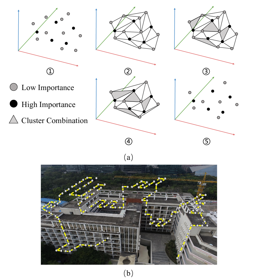
Figure 5: For non-planar flight trajectories, we consider the maximum volume allowed by units that can be combined into evolving clusters. We approximate the local instance space density per unit volume, clustering each point and its neighbors in order of their sizes, and provide a quantifiable information uncertainty measure by combining importance values and relative local density.

In the Voronoi diagram of the data, each point forms its own cell. Next, we approximate the volume of cells. In general, a cell has many neighboring cells with different class labels, and some cells are yet unmarked. Known neighbors are processed in order of their sizes. The considered cell is merged into the neighbor with the smallest class label, and its labeled neighbors also assume the same class. Cells are merged as long as the cell volume remains below the maximum value. After all points have been considered once, all cluster combinations have been executed. However, we still need to perform simple post-processing on the obtained clusters to make them reasonable.

The purpose of point cluster generalization is to correctly convey large-scale information into small-scale information diagrams, considering topological information, and metric information[43] in the process. Based on this, we combine the concepts of importance value and relative local density with the aforementioned cell cluster theory to evaluate the change in the importance value of the entire area and the importance value of the variation. The larger the area of the Voronoi polygon, the greater the weight. Thus, points are more likely to be retained in generalized mapping. The importance value equation is as followed:

$${G_{i}}=\frac{{{\lambda_{i}}{A_{i}}}}{{\sum\limits_{k=1}^{{N_{v}}}{({\lambda_{k}}{A_{k}})}}}$$ (14)

The probability of selecting the specific point, denoted as $G_{i}$, is given by the product of the area of the Voronoi polygon, denoted as $A_{i}$, and the weight value, denoted as $\lambda_{i}$.

Relative local density enables the comparison of density changes point by point before and after generalization, thus better assessing the density changes between points before and after generalization.

$${r_{i}}=\frac{{\frac{1}{{{A_{i}}}}}}{{\sum\limits_{k=1}^{{N_{v}}}{\frac{1}{{{A_{k}}}}}}}$$ (15)

The position information uncertainty of non-planer trajectory is:

$${F_{np}}(I)=\sum\limits_{i=1}^{{N_{v}}}{-\log({G_{i}}){r_{i}}+{\lambda_{i}}{{\left\|{{G_{i}}-{r_{i}}}\right\|}^{2}}}$$ (16)

The positional uncertainty can be expressed as:

$$\sigma_{pos}^{2}(\textsl{I})=\mathbb{I}(p){F_{p}}(\textsl{I})+\mathbb{I}(np){F_{np}}(\textsl{I})$$ (17)

and $\mathbb{I}(\cdot)$ represents the indicator function.

IV-C Implementation

In this section, we will shed some insight on our project. The first introduction is that we propose proportionally distributing samples for improved rendering effects while accelerating sampling based on a threshold. Specifically, we accelerate the process by accumulating transmittance along the ray and terminating sampling beyond a certain threshold.

We also design a classifier to determine whether the trajactory is planar or non. To implement our adaptive classifier, we divide the data point set into two groups, $A={a_{1},...,a_{p}}$ and $B={b_{1},...,b_{q}}$, and measure the similarity between these two sets using the Hausdorff distance. Given two trajectories $A=a_{i}$ and $B=b_{j}$, the Hausdorff distance between sets $A$ and $B$ is defined as:

$$H(A,B)=\max(h(A,B),h(B,A))$$ (18)

, where

$$h(A,B)={\max_{{a_{i}}\in A}}({\min_{{b_{j}}\in B}}\left\|{{a_{i}}-{b_{j}}}\right\|)$$ (19)

Compared to traditional distance metrics, the Hausdorff formula allows direct computation of trajectory similarity without requiring interpolation of trajectory sets, avoiding the addition of noise to trajectory data. By setting a fixed threshold, we can determine the flight trajectory. If the Hausdorff distance between sets $A$ and $B$ exceeds the threshold, indicating low similarity, it can be classified as a non-planar trajectory; otherwise, it is a planar trajectory.

1) Initialization for poses: We input the ground truth RGB images $\{I_{i=1}^{N}\}$ into COLMAP, which is a software to recover the structures from images and output 3D position $\mathbf{x}=(x,y,z)$ in the scene and a viewing direction vector $\mathbf{d}=(\theta,\phi)$.

2) Initialization for NeRF: We randomly select a specific amount of images from dataset to train our weights of NeRF MLP network. Through experiments, we recommend initializing with a quantity that is 10 percent of the total, and an absolute minimum of 20 images.

3) The usage of the variants of NeRFs in our experiments: We use CF-NeRF. ActiveNeRF and D.A.Ensemble as baseline comparisions. In these, ActiveNeRF and CF-NeRF are hard-coded, which change the internal parameters and the uncertainty of the neural network’s output. Thus it cannot be directly embedded into our IOVS framework. However, modifying some of the outputs still allows for integration just as D.A.Ensemble achieves.

4) The stop of our incremental selection: We choose to stop our workflow when a specific reconstruction effect is achieved or a preset limit on the number of selected images is reached.

Algorithm 1 Hybrid-Uncertainty Calculation Algorithm

1:Input: RGB ground truth photos $\{I_{i=1}^{N}\}$

2:Output: hybrid-uncertainty

3:Compute 3D position $\mathbf{x}$, and viewing direction $\mathbf{d}$ using COLMAP

4:Compute volume density $\alpha_{i}$ and color $c(\textbf{r}(t_{i}))$ based on Eq. (4)

5:Compute variance $\beta^{2}(\textbf{r}(t_{i}))$ based on Eq. (8)

6:Construct Beta Distribution based on Eq. (11) and output $\bar{C}(\textbf{r})$, $\bar{\beta}^{2}(\textbf{r})$

7:Compute rendering uncertainty $\sigma^{2}_{rgb}$ using Eq. (7)

8:Compute Hausdorff distance based on Eq. (18)

9:if $h(A,B)<\epsilon$ (a preset threshold) then

10:     Construct Voronoi diagram based on Eq. (12)

11:     Compute planar positional uncertainty based on Eq. (13)

12:else

13:     Construct Voronoi cell and its neighbors

14:     Compute importance value $G_{i}$ based on Eq. (14)

15:     Compute reactive local density $r_{i}$ based on Eq. (15)

16:     Compute non-planar positional uncertainty based on Eq. (16)

17:end if

18:Normalize and compute hybrid-uncertainty based on Eq. (6)

V Experiments

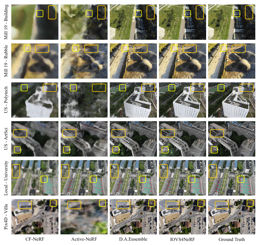
Figure 6: Qualitative results on 6realistic scenes. Several observations can be made: First, IOVS4NeRF performs significantly better than CF-NeRF and Active-NeRF. Also, IOVS4NeRF provides better synthesis quality among the objects with complex textures over D.A.Ensemble and are close to the ground truth.

V-A Experimental Setup

Datasets. Our dataset comprises seven groups: two benchmarks from Mill 19, two from Urban 3D, one from Pix-4D, and two self-captured footage datasets from Changsha, Hunan.

We compare all the methods in the following publicly available large-scale datasets caputred by UAVs:

• Mill19-Building: This dataset comprises 1920 images high resolution of $4608\times 3456$ pixels captured by UAVs within a $0.125\,\text{km}^{2}$ area surrounding an industrial structure .

• Mill19-Rubble: Rubble is a UAV imagery dataset containing 1678 images with 4608$\times$3456 pixel resolution .

• Villa: villa is a UAV photogrametry dataset collected and publiced by Pixel4D, which includes 232 images with the resolution at 6000$\times$4000 pixels .

• UrbanScene3D-Polytech and UrbanScene3D-Artsci: UrbanScene3D is a large-scale data platform for urban scene perception and reconstruction, encompassing over 128,000 high-resolution images across 16 scenes, covering a total area of 136 square kilometers . Polytech and Artsci are subsets of UrbanScene3D, providing LiDAR scans and image sets. Specifically, polytech contains 798 UAV filmed images at 4864$\times$3648 pixels resolution while Artsci has 989 images at 5472$\times$3648 pixels resolution .

• CSC-university and CSC-Lake: Both are self-collected UAV imagery datasets. CSC-university includes 391 images with resolution at 4000$\times$3000 pixels covering $0.1km^{2}$. While CSC-Lake contains 211 images with resolution at 4000$\times$3000 pixels covering $0.9km^{2}$ .

Metrics. Note that this work focuses on optimal view selection with hybrid-uncertainty estimation. Thus, our evaluation metrics are divided into two types.

1) In the uncertainty estimation experiments, we evaluate the proposed against the existing works by comparing the prediction accuracy of uncertainty:

• SRCC[44]: We use Spearman’s rank correlation coefficient (SRCC) to measure the monotonic relationship between average uncertainty estimation on test views and rendering errors.

• AUSE[45]: We report the Area Under the Sparsification Error (AUSE) curve to evaluate structural similarity, which reveals the degree to which uncertainty matches rendering errors on pixels.

2) In novel view synthesis experiments, we evaluate the proposed against the existing works by comparing the following three metrics:

• PSNR: Peak Signal-to-Noise Ratio (PSNR) is a classic metric for measuring image reconstruction quality.

• SSIM[46]: Structural Similarity Index (SSIM) is a metric for measuring structural similarity between two images.

• LPIPS[47]: Learned Perceptual Image Patch Similarity (LPIPS) is a learning-based metric that considers perceptual characteristics of the human visual system, which is widely used to measure perceptual differences between two images.

Comparison methods. We compare the proposed solution IOVS4NeRF over three state-of-the-art large-scale NeRF solutions with a dynamic view selection strategy to leverage the reconstruction quality and computational consuming:

• CF-NeRF[48] : CF-NeRF is a probabilistic framework that incorporates uncertainty quantification into NeRF by learning a distribution over all possible radiance fields, enabling reliable uncertainty estimation while maintaining model expressivity.

• Active-NeRF [26] : ActiveNeRF is a learning framework designed to model 3D scenes with a constrained input budget by incorporating uncertainty estimation into a NeRF model, ensuring robustness with few observations and providing scene interpretation.

• D.A.Ensemble[14] : D.A.Ensemble quantifies model uncertainty in NeRF by incorporating a density-aware epistemic uncertainty term that considers termination probabilities along individual rays to identify uncertainty from unobserved parts of a scene, achieving SOTA performance in uncertainty quantification benchmarks and supporting next-best view selection and model refinement.

Setup Details. We utilize the Instant-NGP [17] to demonstrate the effectiveness of the proposed IOVS4NeRF. But please note that as we illustrate in section XXX we can replace Instant-NGP with any NeRF solutions (supplemental material). All the experiments are conducted with a Intel core I9 CPU and an NVIDIA GeForce 3090 GPU (24GB memory).

TABLE I: Quantitative results in 6 real image scens: IOVS4NeRF performs superior to or on par with the three state-of-the-art related solutions CF-NeRF, Active-NeRF and D.A.Ensenble in the quality of synthesized novel views (PSNR, SSIM and LPIPS), the accuracy of uncertainty estimation (AUSE and SRCC) and the efficiency (time-consuming). The best and second results are shown in green and blue, respectively.

Scenes	Methods	Quality Metrics			Uncertainty Metrics		Time↓
		PSNR↑	SSIM↑	LPIPS↓	AUSE↓	SRCC↑
Building	CF-NeRF	14.926	0.260	0.738	0.100	0.706	12:57:17
	Active-NeRF	12.430	0.231	0.777	0.141	0.464	17:45:19
	D.A.Ensemble	16.857	0.383	0.422	0.303	0.668	12:18:28
	IOVS4NeRF	19.841	0.469	0.351	0.055	0.878	7:28:20
Rubble	CF-NeRF	17.758	0.312	0.717	0.075	0.815	12:58:39
	Active-NeRF	16.531	0.275	0.622	0.097	0.683	17:47:24
	D.A.Ensemble	19.629	0.507	0.335	0.257	0.818	12:20:52
	IOVS4NeRF	21.108	0.573	0.303	0.052	0.884	7:29:14
Polytech	CF-NeRF	14.259	0.251	0.731	0.118	0.751	12:57:28
	Active-NeRF	8.888	0.153	0.747	0.264	-0.035	17:46:55
	D.A.Ensemble	20.673	0.564	0.253	0.058	0.915	12:46:18
	IOVS4NeRF	21.810	0.592	0.235	0.053	0.925	7:48:22
ArtSci	CF-NeRF	15.578	0.227	0.693	0.106	0.729	12:57:14
	Active-NeRF	13.531	0.193	0.610	0.152	0.525	17:48:20
	D.A.Ensemble	17.769	0.463	0.338	0.101	0.793	13:28:42
	IOVS4NeRF	18.836	0.500	0.319	0.083	0.834	8:21:14
University	CF-NeRF	15.359	0.189	0.669	0.112	0.645	12:58:12
	Active-NeRF	17.814	0.359	0.359	0.087	0.780	17:46:50
	D.A.Ensemble	16.610	0.331	0.416	0.101	0.682	12:08:12
	IOVS4NeRF	18.722	0.430	0.327	0.077	0.814	6:47:53
Villa	CF-NeRF	15.141	0.259	0.645	0.111	0.777	12:58:44
	Active-NeRF	9.236	0.121	0.828	0.242	0.055	20:32:57
	D.A.Ensemble	15.415	0.337	0.494	0.123	0.689	13:58:26
	IOVS4NeRF	18.250	0.457	0.386	0.079	0.868	8:46:40

V-B Evaluation of Uncertainty Estimation

Our first experiment is to demonstrate that our uncertainty estimation strongly correlates with novel view synthesis quality for NeRFs. To evaluate the quality of uncertainty prediction, we consider two metrics, namely, SRCC and AUSE, that are widely used in existing next-best view selection solution [11].

For each dataset, we generate 100 test sets. Each set contains four randomly selected images from the scene, with three used as reference images and the fourth as the test view. We calculate the average predicted uncertainty and mean squared error (MSE) for each test view. Subsequently, we determine the SRCC values for the 100 pairs of averaged uncertainty and MSE. SRCC values above 0.8 empirically indicate a strong monotonic relationship (higher average uncertainty predictions correspond to higher average rendering errors). Additionally, we report the average AUSE across 100 test views for each scene. An AUSE of 0 signifies that the pixel-wise uncertainty magnitudes are perfectly aligned with the MSE values (uncertain areas in the rendered test view coincide with erroneous predictions).

We compare IOVS4NeRF against three SOTA NeRF-Based view selection solutions. As shown in Table. I, IOVS4NeRF achieves significant more information in uncertainty prediction with respect to synthesis error over CF-NeRF, Active-NeRF and D.A.Ensemble. The superior performance of our the approach demonstrates the proposed hybrid-uncertainty leads to more consistent uncertainty estimates compared to solely rendering-based uncertainty such as CF-NeRF, Active-NeRF, and D.A.Ensemble.

V-C Evaluation of Novel View Synthesis

In this section, we evaluate the proposed method via the quality of novel view synthesis. Specifically, we compare IOVS4NeRF against optimal view selection baselines and state-of-the-art solutions.

For each dataset, due to GPU limitations, we randomly select 500 images as the full image set (if the total number of image in a dataset is less than 500, we use all the images instead). We randomly choose 15% of the images in each dataset for initialization and randomly select 10% of the images as the test set. Then we incrementally select 15% of the images using vrious view selection methods as the optimal views for incremental training. Thus, only 30% of the full image set are used to synthesis the novel view, of which quality are evaluted by using PSNR, SSIM and LPIPS.

TABLE II: Quantitative comparison of IOVS4NeRF against to two baselined view selection strategies random and FVS on the ArtSci dataset. We report the average PSNR, SSIM and LPIPS scores of the synthesized novel views by using the incremental select 15% images. Note that only 30% of the full image set is used for IOVS4NeRF, random and FVS. Our proposed approach IOVS4NeRF finds informative images in the scene, and provides the best performance. The best and second results are shown in green and blue, respectively.

		Building	Rubble	Polytech	ArtSci	Villa	University
Random	PSNR$\uparrow$	16.857	18.959	20.245	17.281	14.547	16.093
	SSIM$\uparrow$	0.383	0.500	0.554	0.444	0.307	0.305
	LPIPS$\downarrow$	0.422	0.330	0.266	0.348	0.527	0.447
FVS	PSNR$\uparrow$	17.272	20.045	18.606	17.687	15.917	16.338
	SSIM$\uparrow$	0.368	0.491	0.534	0.451	0.360	0.305
	LPIPS$\downarrow$	0.428	0.341	0.283	0.352	0.475	0.443
Ours	PSNR$\uparrow$	19.841	21.108	21.810	18.836	18.250	18.722
	SSIM$\uparrow$	0.469	0.573	0.592	0.500	0.457	0.430
	LPIPS$\downarrow$	0.351	0.303	0.265	0.319	0.386	0.327
Full	PSNR$\uparrow$	20.547	22.613	22.661	19.408	19.509	19.666
	SSIM$\uparrow$	0.525	0.592	0.619	0.538	0.485	0.463
	LPIPS$\downarrow$	0.319	0.265	0.220	0.306	0.387	0.322

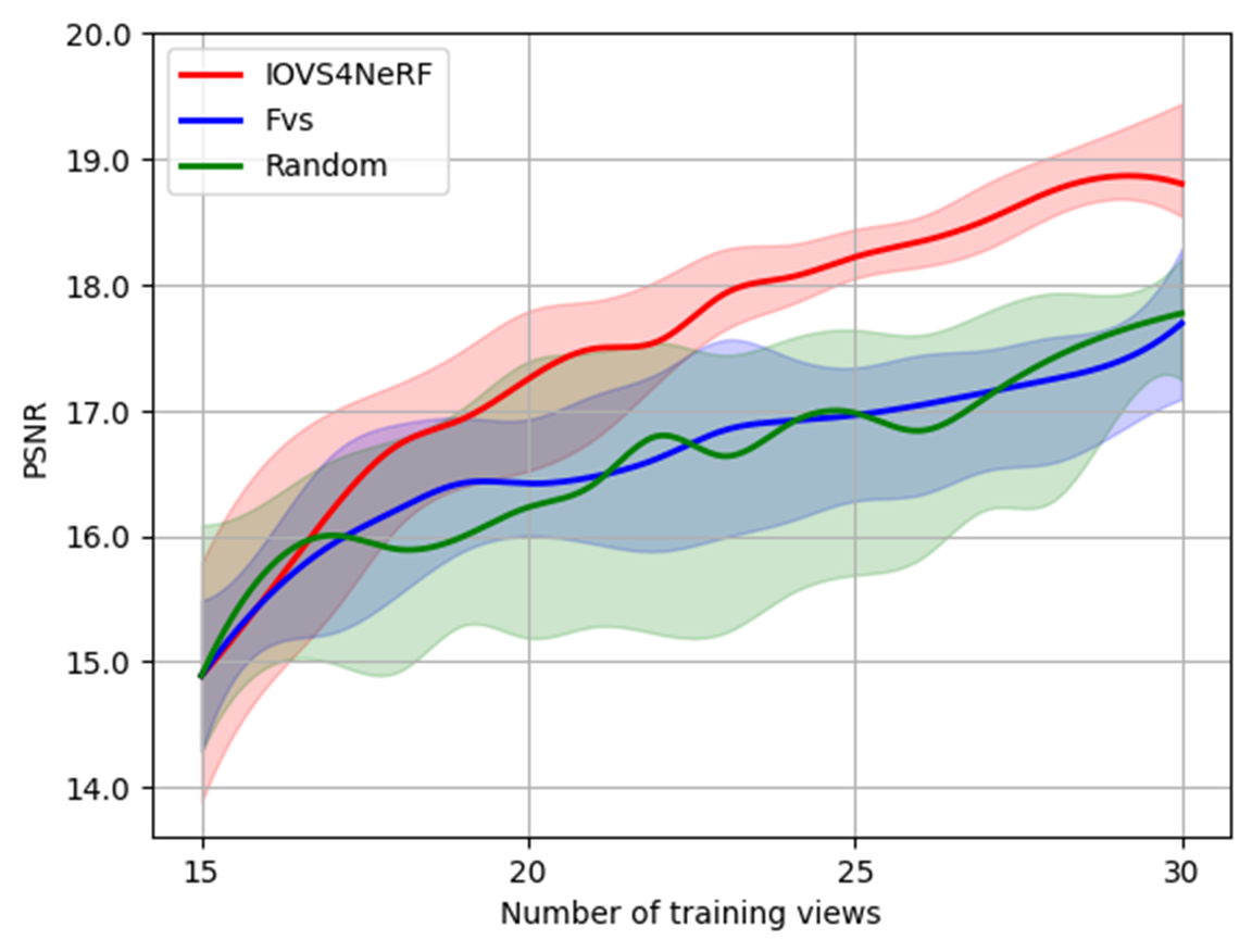
Figure 7: Comparison of IOVS4NeRF against to two baselined view selection strategies random and FVS on the ArtSci dataset. For each test scene, we incrementally re-train the instan-NGP model by adding the new views selected by IOVS4NeRF, random and FVS at each step, then render tested views and report the average PSNR scores with standard deviations over all test scenes and runs respectively. Note that the large standard deviations are due to the varying rendering difficulty of each scene. Our proposed approach IOVS4NeRF finds informative images in the scene, improving scene representations via image-based neural rendering.

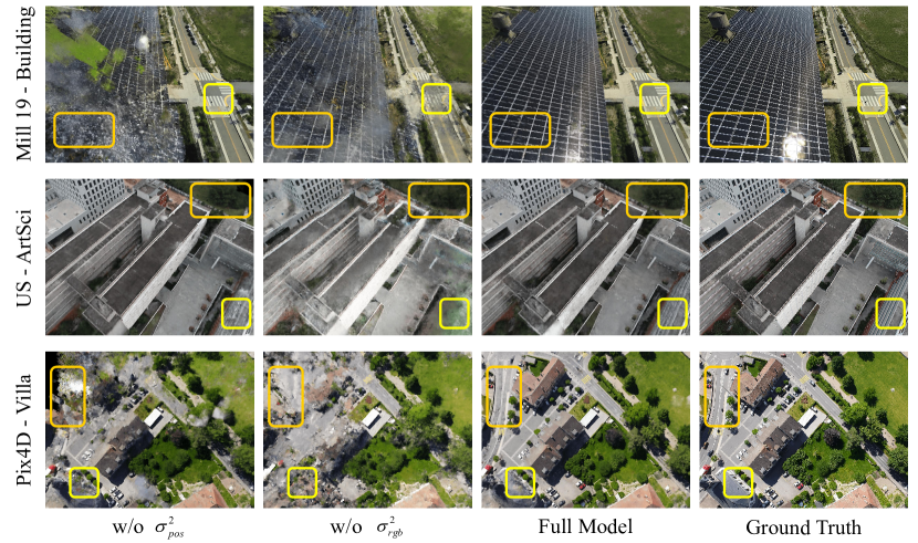
Figure 8: Qualitative comparisons in ablation study by removing the rendering uncertainty $\sigma_{rgb}^{2}$ and positional uncertainty $\sigma_{pos}^{2}$ in proposed hybrid-uncertainty one by one.

(1) Comparison of Baseline Optimal View Selection Strategies: We compare the proposed optimal view selection approach IOV4NeRF against two heuristic baselines:

• Random: selects a view candidate uniformly at random.

• FVS: selects the view that maximizes the view distance with respect to previously collected images.

As shown in Fig. 7, the rendering quality (PSNR score) of the ArtSci dataset by all three methods keeps growing with the increasing number of selected views. However, the PSNR of IOVS4NeRF raises significantly faster over FVS and random which indicates that our approach is capable of selecting informative views.

As shown in Table. II that IOVS4NeRF outperforms FVS and random in PSNR, SSIM and LPIPS by a significant margin, with the rendering quality close to the results trained with the full image sets. The quantitative results in Table. II also verify the effectiveness of the proposed IOVS4NeRF over the baseline strategies.

(2) Comparison of State-of-the-art Optimal View Selection: We validate the performance of our proposed framework, IOVS4NeRF, and compare it with three state-of-the-art NeRF-based optimal view selection solutions, namely, CF-NeRF, Active-NeRF and D.A.Ensemble.

We first show the results with an incremental learning scheme, where the time and computation resources are considered sufficient. As shown in Figure. 6, we can easily see that IOVS4NeRF generate better visual quality synthesized novel views against the outputs of CF-NeRF, Active-NeRF and D.A.Ensemble, that are closed to the ground truth among all 6 datesets. The quantitative results in Table. I also show IOVS4NeRF achieves the best performance in three synthesis image quality evaluation metrics (PSNR, SSIM, LPIPS) over the CF-NeRF, Active-NeRF and D.A.Ensemble. These experimental observations prove the proposed method IOVS4NeRF can select most informative inputs compared with state-of-the-art approaches, which contributes most to synthesizing views from less observed regions.

The runtime comparison in Table. I shows that IOVS4NeRF outperforms CF-NeRF, Active-NeRF and D.A.Ensemble in efficiency with a significant margin. We interpret this acceleration are mainly due to all three compared optimal view selection strategies in CF-NeRF, Active-NeRF and D.A.Ensemble are hard-coded with a NeRF module while IOVS4NeRF is a flexible framework where the proposed hybrid-uncertainty computation is as a plug-in to any NeRF solution (e.g. Instant-NGP in our experiment). This soft-coded scheme leads to an advantage in efficiency. It is vital to notice that once a more advanced NeRF solution be developed in the future, it can be easily applied in IOVS4NeRF and is supposed to achieve further improvements in both synthesize quality and time-consuming.

TABLE III: Ablation on hybrid-uncertainty by removing the rendering uncertainty $\sigma_{rgb}^{2}$ and positional uncertainty $\sigma_{pos}^{2}$ one by one. The best and second results are shown in green and blue, respectively.

		Building	Rubble	Polytech	ArtSci	Villa	University
w/o $\sigma_{pos}^{2}$	PSNR$\uparrow$	17.031	19.803	19.856	18.386	15.937	16.782
	SSIM$\uparrow$	0.404	0.527	0.541	0.497	0.356	0.329
	LPIPS$\downarrow$	0.407	0.645	0.731	0.693	0.645	0.669
w/o $\sigma_{rgb}^{2}$	PSNR$\uparrow$	17.841	20.045	18.606	17.687	15.917	16.338
	SSIM$\uparrow$	0.390	0.491	0.534	0.451	0.368	0.305
	LPIPS$\downarrow$	0.421	0.341	0.534	0.352	0.475	0.443
Full Model	PSNR$\uparrow$	19.841	21.108	21.810	18.836	18.250	18.722
	SSIM$\uparrow$	0.469	0.573	0.592	0.500	0.457	0.430
	LPIPS$\downarrow$	0.351	0.303	0.235	0.319	0.386	0.327

V-D Ablations Study

Note that in this paper, we propose to use hybrid-uncertainty over the solely rendering uncertainty that is widely used in existing works. Thus, in this experiment, we further evaluate the effectiveness of the candidate uncertainty estimation module alone.

We denote the baseline approaches as:

• w/o $\sigma_{pos}^{2}$: IOVS4NeRF with rendering uncertainty $\sigma_{rgb}^{2}$ only by removing the positional uncertainty term $\sigma_{pos}^{2}$ in Eq. (6).

• w/o $\sigma_{rgb}^{2}$: IOVS4NeRF with positional uncertainty $\sigma_{pos}^{2}$ only by removing the rendering uncertainty term $\sigma_{rgb}^{2}$ in Eq. (6).

• Full Model: IOVS4NeRF with completed hybrid-uncertainty computation strategy shown in Eq. (6).

The quantitative experimental results are shown in Table. III while the qualitative experimental results are shown in Figure. 8. Both comparisons show that IOVS4NeRF obviously outperforms ablated approaches consistently which indicates that both rendering uncertainty $\sigma_{rgb}^{2}$ and positional uncertainty $\sigma_{pos}^{2}$ contributes to the uncertainty estimation of the candidate view and improve the capability of informative view selection.

V-E Benefit to Classical Photogrammetry Solutions

Note that the proposed approach IOVS4NeRF is a flexible framework to assist NeRF-based novel view synthesis. It is interesting if IOVS4NeRF can assist the classical photogrammetry pipeline. In this experiment, we use the selected views by IOVS4NeRF, random, FVS and completed image set Full as input to famous commercial photogrammetry software MestShape to perform the dense 3D reconstruction pipeline for comparison. Specifically, we randomly 25% images in Lake and Polytech datasets as initialization and select 25% views in the rest set by using IOVS4NeRF, random, FVS for incrementally re-training. The results in Figure. 9 show that the reconstructed scenes by using the selected views from random, FVS are with obvious artifacts. In contrast, the selected views by IOVS4NeRF lead to similar 3D reconstruction quality as the ones using Full image sets as input for MetaShape but with only half processing time. This experiment demonstrates IOVS4NeRF not only can ameliorate the novel view synthesis task by using NeRFs, but also benefit the classical photogrammetry solutions.

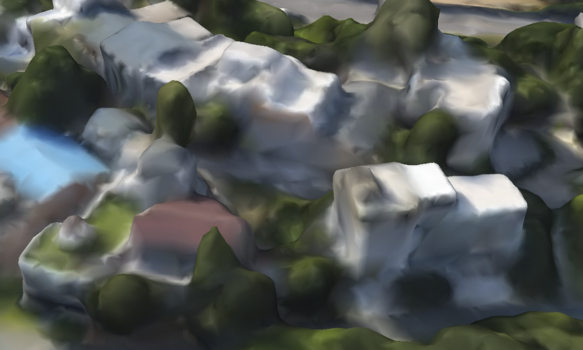
Lake : Random

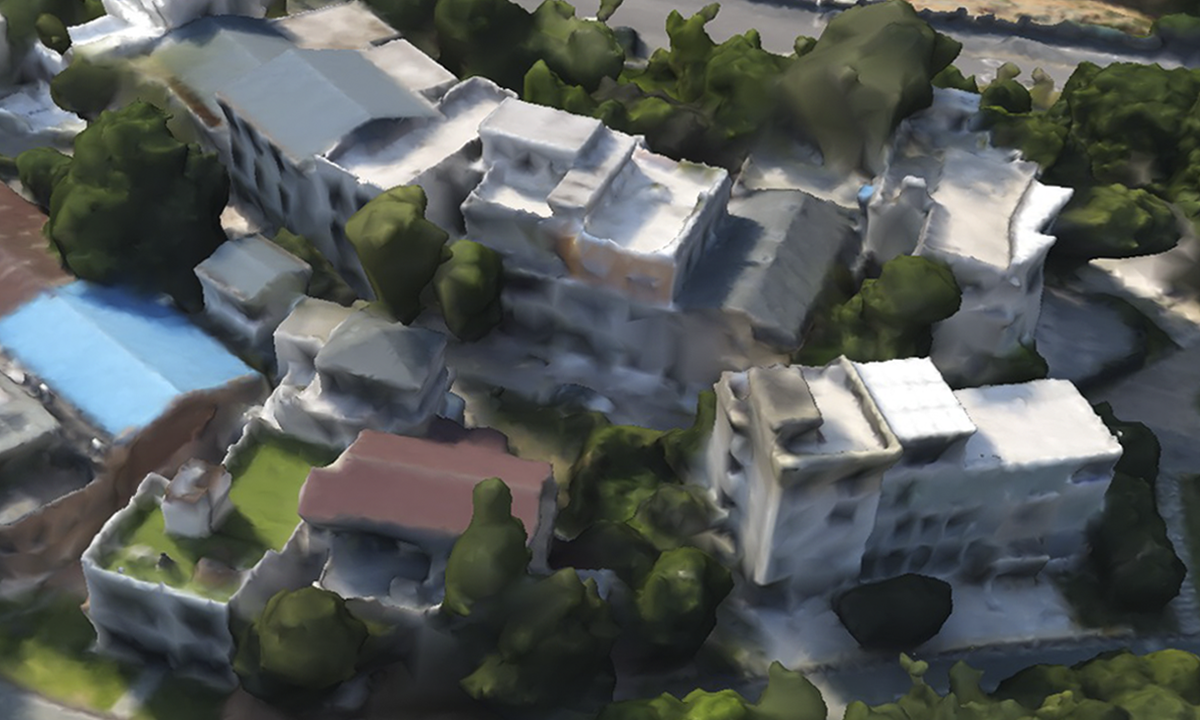
Lake : FVS

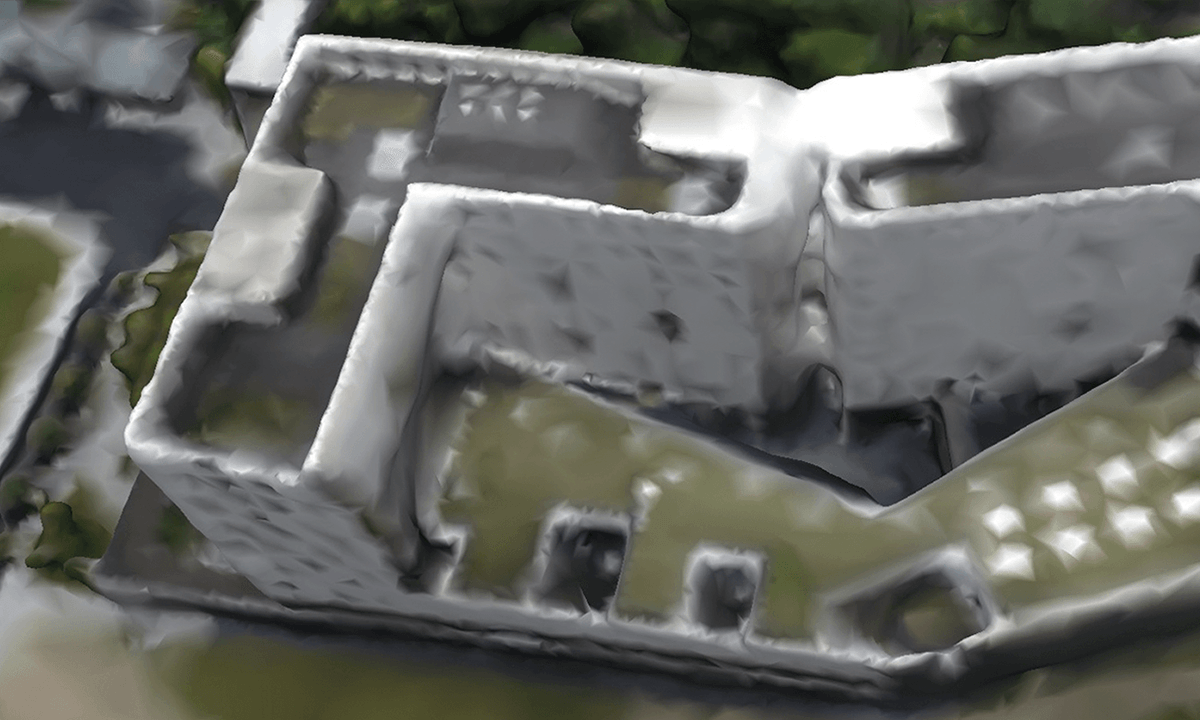
Polytech : Random

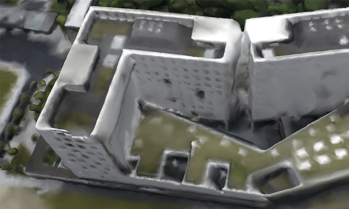
Polytech : FVS

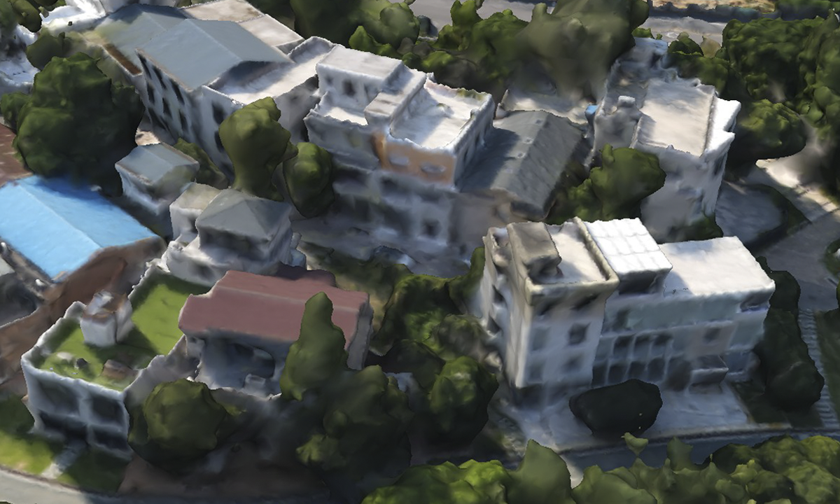
Lake : IOVS4NeRF

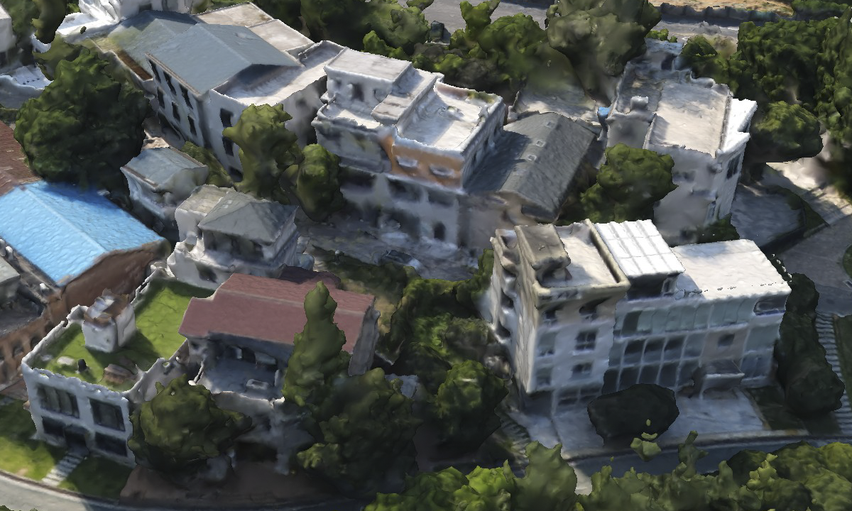
Lake : Full

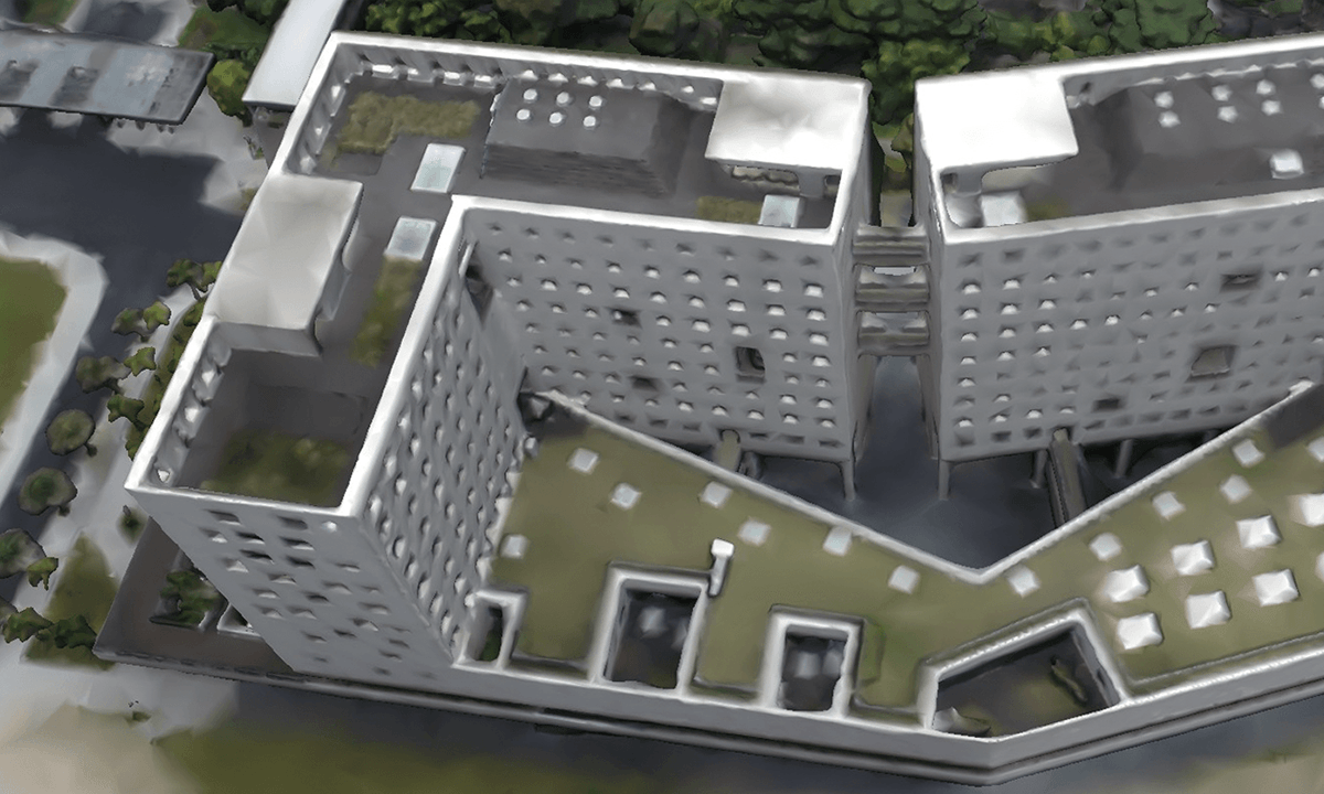
Polytech : IOVS4NeRF

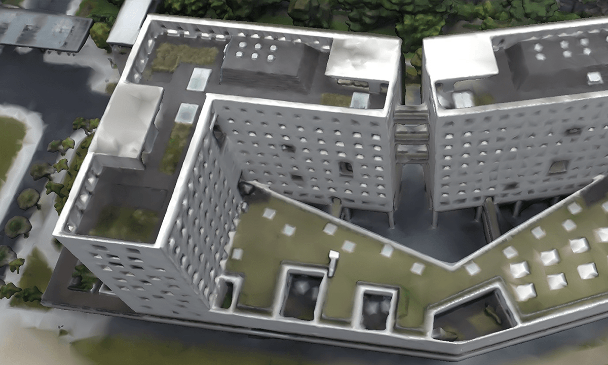
Polytech : Full

Figure 9: Verification of the capability of the proposed method IOVS4NeRF to benefit classical photogrammetry. Several observations can be made: the selected views by IOVS4NeRF lead to similar 3D reconstruction quality as the ones using Full image sets as input for MetaShape but with only half processing time.

VI Conclusion

In this work, we present a novel framework method, IOVS4NeRF, with the goal of rendering large-scale urban scenes. Our approach builds upon the original NeRF architecture by using Instant-NGP for assistance, which incorporates enhanced explicit-implicit fusion for information storage and lightweight neural MLP networks can accelerate the overall reconstruction speed. The threshold sampling with joint rendering of uncertainty and Voronoi graph perception can improve overall rendering quality, making them suitable for large-scale 3D reconstruction tasks.

When applied to extensive urban landscapes, our approach overcomes the limitations of existing methods. Our model achieves high visual fidelity rendering even in extremely large-scale city scenes, a critical capability for real-world applications. Empirical evaluations of our fast renderer based on our framework suggest that interactive large-scale rendering remains an open research challenge. Our model inherits some limitations from NeRF-based approaches, such as handling a large number of high-resolution images, indicating areas for further refinement in future work.

VII Acknowledgement

This project is supported by Provincial Natural Science Foundation of Hunan(2024JJ10027) .

References

- [1] C. B. Choy, D. Xu, J. Gwak, K. Chen, and S. Savarese, “3d-r2n2: A unified approach for single and multi-view 3d object reconstruction,” in Computer Vision–ECCV 2016: 14th European Conference, Amsterdam, The Netherlands, October 11-14, 2016, Proceedings, Part VIII 14. Springer, 2016, pp. 628–644.
- [2] N. Wang, Y. Zhang, Z. Li, Y. Fu, W. Liu, and Y.-G. Jiang, “Pixel2mesh: Generating 3d mesh models from single rgb images,” in Proceedings of the European conference on computer vision (ECCV), 2018, pp. 52–67.
- [3] H. Fan, H. Su, and L. J. Guibas, “A point set generation network for 3d object reconstruction from a single image,” in Proceedings of the IEEE conference on computer vision and pattern recognition, 2017, pp. 605–613.
- [4] R. Chen, S. Han, J. Xu, and H. Su, “Point-based multi-view stereo network,” in Proceedings of the IEEE/CVF international conference on computer vision, 2019, pp. 1538–1547.
- [5] B. Mildenhall, P. P. Srinivasan, M. Tancik, J. T. Barron, R. Ramamoorthi, and R. Ng, “Nerf: Representing scenes as neural radiance fields for view synthesis,” Communications of the ACM, vol. 65, no. 1, pp. 99–106, 2021.
- [6] A. Yu, V. Ye, M. Tancik, and A. Kanazawa, “pixelnerf: Neural radiance fields from one or few images,” in Proceedings of the IEEE/CVF Conference on Computer Vision and Pattern Recognition, 2021, pp. 4578–4587.
- [7] L. Paull, G. Huang, and J. J. Leonard, “A unified resource-constrained framework for graph slam,” in 2016 IEEE International Conference on Robotics and Automation (ICRA). IEEE, 2016, pp. 1346–1353.
- [8] A. Torres-González, J. R. Martínez-de Dios, and A. Ollero, “Robot-beacon distributed range-only slam for resource-constrained operation,” Sensors, vol. 17, no. 4, p. 903, 2017.
- [9] R. Zeng, Y. Wen, W. Zhao, and Y.-J. Liu, “View planning in robot active vision: A survey of systems, algorithms, and applications,” Computational Visual Media, vol. 6, pp. 225–245, 2020.
- [10] D. Peralta, J. Casimiro, A. M. Nilles, J. A. Aguilar, R. Atienza, and R. Cajote, “Next-best view policy for 3d reconstruction,” in Computer Vision–ECCV 2020 Workshops: Glasgow, UK, August 23–28, 2020, Proceedings, Part IV 16. Springer, 2020, pp. 558–573.
- [11] L. Jin, X. Chen, J. R”̈uckin, and M. Popović, “Neu-nbv: Next best view planning using uncertainty estimation in image-based neural rendering,” arXiv preprint arXiv:2303.01284, 2023.
- [12] J. Shen, A. Ruiz, A. Agudo, and F. Moreno-Noguer, “Stochastic neural radiance fields: Quantifying uncertainty in implicit 3d representations,” in 2021 International Conference on 3D Vision (3DV). IEEE, 2021, pp. 972–981.
- [13] Y. Gal and Z. Ghahramani, “Dropout as a bayesian approximation: Representing model uncertainty in deep learning,” in international conference on machine learning. PMLR, 2016, pp. 1050–1059.
- [14] N. S”̈underhauf, J. Abou-Chakra, and D. Miller, “Density-aware nerf ensembles: Quantifying predictive uncertainty in neural radiance fields,” in 2023 IEEE International Conference on Robotics and Automation (ICRA). IEEE, 2023, pp. 9370–9376.
- [15] M. Roberts, D. Dey, A. Truong, S. Sinha, S. Shah, A. Kapoor, P. Hanrahan, and N. Joshi, “Submodular trajectory optimization for aerial 3d scanning,” in Proceedings of the IEEE International Conference on Computer Vision, 2017, pp. 5324–5333.
- [16] G. Petrie, “Systematic oblique aerial photography using multiple digital cameras,” Photogrammetric Engineering & Remote Sensing, vol. 75, no. 2, pp. 102–107, 2009.
- [17] T. M”̈uller, A. Evans, C. Schied, and A. Keller, “Instant neural graphics primitives with a multiresolution hash encoding,” ACM Transactions on Graphics (ToG), vol. 41, no. 4, pp. 1–15, 2022.
- [18] K. Khosoussi, M. Giamou, G. S. Sukhatme, S. Huang, G. Dissanayake, and J. P. How, “Reliable graphs for slam,” The International Journal of Robotics Research, vol. 38, no. 2-3, pp. 260–298, 2019.
- [19] S. Ullman, “The interpretation of structure from motion,” Proceedings of the Royal Society of London. Series B. Biological Sciences, vol. 203, no. 1153, pp. 405–426, 1979.
- [20] Y. Furukawa, C. Hernández et al., “Multi-view stereo: A tutorial,” Foundations and Trends® in Computer Graphics and Vision, vol. 9, no. 1-2, pp. 1–148, 2015.
- [21] S. P. Lim and H. Haron, “Surface reconstruction techniques: a review,” Artificial Intelligence Review, vol. 42, pp. 59–78, 2014.
- [22] S. Wang, R. Clark, H. Wen, and N. Trigoni, “Deepvo: Towards end-to-end visual odometry with deep recurrent convolutional neural networks,” in 2017 IEEE international conference on robotics and automation (ICRA). IEEE, 2017, pp. 2043–2050.
- [23] C. Tang and P. Tan, “Ba-net: Dense bundle adjustment network,” arXiv preprint arXiv:1806.04807, 2018.
- [24] D. J. MacKay, “Bayesian neural networks and density networks,” Nuclear Instruments and Methods in Physics Research Section A: Accelerators, Spectrometers, Detectors and Associated Equipment, vol. 354, no. 1, pp. 73–80, 1995.
- [25] D. P. Kingma, T. Salimans, and M. Welling, “Variational dropout and the local reparameterization trick,” Advances in neural information processing systems, vol. 28, 2015.
- [26] R. Martin-Brualla, N. Radwan, M. S. Sajjadi, J. T. Barron, A. Dosovitskiy, and D. Duckworth, “Nerf in the wild: Neural radiance fields for unconstrained photo collections,” in Proceedings of the IEEE/CVF Conference on Computer Vision and Pattern Recognition, 2021, pp. 7210–7219.
- [27] X. Pan, Z. Lai, S. Song, and G. Huang, “Activenerf: Learning where to see with uncertainty estimation,” in European Conference on Computer Vision. Springer, 2022, pp. 230–246.
- [28] W. Hu, Y. Wang, L. Ma, B. Yang, L. Gao, X. Liu, and Y. Ma, “Tri-miprf: Tri-mip representation for efficient anti-aliasing neural radiance fields,” in Proceedings of the IEEE/CVF International Conference on Computer Vision, 2023, pp. 19 774–19 783.
- [29] W. Bian, Z. Wang, K. Li, J.-W. Bian, and V. A. Prisacariu, “Nope-nerf: Optimising neural radiance field with no pose prior,” in Proceedings of the IEEE/CVF Conference on Computer Vision and Pattern Recognition, 2023, pp. 4160–4169.
- [30] H. Koivistoinen, M. Ruuska, and T. Elomaa, “A voronoi diagram approach to autonomous clustering,” in Discovery Science: 9th International Conference, DS 2006, Barcelona, Spain, October 7-10, 2006. Proceedings 9. Springer, 2006, pp. 149–160.
- [31] X. Xie, R. Cheng, M. L. Yiu, L. Sun, and J. Chen, “Uv-diagram: A voronoi diagram for uncertain spatial databases,” The VLDB journal, vol. 22, no. 3, pp. 319–344, 2013.
- [32] Y. Xiangli, L. Xu, X. Pan, N. Zhao, A. Rao, C. Theobalt, B. Dai, and D. Lin, “Bungeenerf: Progressive neural radiance field for extreme multi-scale scene rendering,” in European conference on computer vision. Springer, 2022, pp. 106–122.
- [33] H. Turki, D. Ramanan, and M. Satyanarayanan, “Mega-nerf: Scalable construction of large-scale nerfs for virtual fly-throughs,” in Proceedings of the IEEE/CVF Conference on Computer Vision and Pattern Recognition, 2022, pp. 12 922–12 931.
- [34] L. Xu, Y. Xiangli, S. Peng, X. Pan, N. Zhao, C. Theobalt, B. Dai, and D. Lin, “Grid-guided neural radiance fields for large urban scenes,” in Proceedings of the IEEE/CVF Conference on Computer Vision and Pattern Recognition, 2023, pp. 8296–8306.
- [35] F. Lu, Y. Xu, G. Chen, H. Li, K.-Y. Lin, and C. Jiang, “Urban radiance field representation with deformable neural mesh primitives,” in Proceedings of the IEEE/CVF International Conference on Computer Vision, 2023, pp. 465–476.
- [36] M. Tancik, V. Casser, X. Yan, S. Pradhan, B. Mildenhall, P. P. Srinivasan, J. T. Barron, and H. Kretzschmar, “Block-nerf: Scalable large scene neural view synthesis,” in Proceedings of the IEEE/CVF Conference on Computer Vision and Pattern Recognition, 2022, pp. 8248–8258.
- [37] K. Zhang, G. Riegler, N. Snavely, and V. Koltun, “Nerf++: Analyzing and improving neural radiance fields,” arXiv preprint arXiv:2010.07492, 2020.
- [38] A. Kendall and Y. Gal, “What uncertainties do we need in bayesian deep learning for computer vision?” Advances in neural information processing systems, vol. 30, 2017.
- [39] J. B. McDonald and Y. J. Xu, “A generalization of the beta distribution with applications,” Journal of Econometrics, vol. 66, no. 1-2, pp. 133–152, 1995.
- [40] X. Yuan, C. Chen, M. Jiang, and Y. Yuan, “Prediction interval of wind power using parameter optimized beta distribution based lstm model,” Applied Soft Computing, vol. 82, p. 105550, 2019.
- [41] S. Rokhsaritalemi, A. Sadeghi-Niaraki, and S.-M. Choi, “Drone trajectory planning based on geographic information system for 3d urban modeling,” in 2018 International Conference on Information and Communication Technology Convergence (ICTC). IEEE, 2018, pp. 1080–1083.
- [42] K. Ok, S. Ansari, B. Gallagher, W. Sica, F. Dellaert, and M. Stilman, “Path planning with uncertainty: Voronoi uncertainty fields,” in 2013 IEEE International Conference on Robotics and Automation. IEEE, 2013, pp. 4596–4601.
- [43] H. Yan and R. Weibel, “An algorithm for point cluster generalization based on the voronoi diagram,” Computers & Geosciences, vol. 34, no. 8, pp. 939–954, 2008.
- [44] C. Spearman, “The proof and measurement of association between two things.” 1961.
- [45] E. Ilg, O. Cicek, S. Galesso, A. Klein, O. Makansi, F. Hutter, and T. Brox, “Uncertainty estimates and multi-hypotheses networks for optical flow,” in Proceedings of the European Conference on Computer Vision (ECCV), 2018, pp. 652–667.
- [46] Z. Wang, A. C. Bovik, H. R. Sheikh, and E. P. Simoncelli, “Image quality assessment: from error visibility to structural similarity,” IEEE transactions on image processing, vol. 13, no. 4, pp. 600–612, 2004.
- [47] R. Zhang, P. Isola, A. A. Efros, E. Shechtman, and O. Wang, “The unreasonable effectiveness of deep features as a perceptual metric,” in Proceedings of the IEEE conference on computer vision and pattern recognition, 2018, pp. 586–595.
- [48] J. Shen, A. Agudo, F. Moreno-Noguer, and A. Ruiz, “Conditional-flow nerf: Accurate 3d modelling with reliable uncertainty quantification,” in European Conference on Computer Vision. Springer, 2022, pp. 540–557.