Denoising Lévy Probabilistic Models

Abstract

Investigating the noise distribution beyond Gaussian in diffusion generative models remains an open problem. The Gaussian case has been a large success experimentally and theoretically, admitting a unified stochastic differential equation (SDE) framework, encompassing score-based and denoising formulations. Recent studies have investigated the potential of heavy-tailed noise distributions to mitigate mode collapse and effectively manage datasets exhibiting class imbalance, heavy tails, or prominent outliers. Very recently, Yoon et al. (NeurIPS 2023), presented the Levy-Ito model (LIM) that directly extended the SDE-based framework, to a class of heavy-tailed SDEs, where the injected noise followed an $\alpha$-stable distribution – a rich class of heavy-tailed distributions. Despite its theoretical elegance and performance improvements, LIM relies on highly involved mathematical techniques, which may limit its accessibility and hinder its broader adoption and further development. In this study, we take a step back, and instead of starting from the SDE formulation, we extend the denoising diffusion probabilistic model (DDPM) by directly replacing the Gaussian noise with $\alpha$-stable noise. We show that, by using only elementary proof techniques, the proposed approach, denoising Lévy probabilistic model (DLPM) algorithmically boils down to running vanilla DDPM with minor modifications, hence allowing the use of existing implementations with minimal changes. Remarkably, as opposed to the Gaussian case, DLPM and LIM yield different backward processes leading to distinct sampling algorithms. This fundamental difference translates favorably for the performance of DLPM in various aspects: our experiments show that DLPM achieves better coverage of the tails of the data distribution, better generation of unbalanced datasets, and improved computation times requiring significantly smaller number of backward steps. The source code will be publicly available at https://github.com/darioShar/DLPM.

1 Introduction

The evolution of generative modeling has seen the emergence of multiple approaches. The current most popular one, diffusion models, designate a family of methods that transport the data distribution to a Gaussian distribution, using a forward noising process, and then learn to reverse this process. The first significant direction of research was the denoising formulation. It was first presented in the deep unsupervised learning context by Sohl-Dickstein et al. (2015). Here, given a data point $X_{0}\sim p_{\star}$ coming from an unknown data distribution $p_{\star}$ (e.g., from an image dataset) one first defines a forward process:

$$X_{t+1}=\gamma_{t}X_{t}+\sigma_{t}\epsilon_{t}\;,$$ (1)

where $X_{t}\in\mathbb{R}^{d}$, $\gamma_{t},\sigma_{t}\in\mathbb{R}_{+}$ are scale variables, and $\epsilon_{t}$ is some multivariate Gaussian noise added at step $t$ so that the distribution of $X_{t}$ becomes ‘more and more Gaussian’ as $t$ increases. Then, the goal becomes to identify the reverse of this process, namely the backward process, so that once some random Gaussian noise is given, the reverse process takes the noise back to the data distribution, hence generating a new data sample.

Subsequently, the development of denoising diffusion probabilistic models (DDPM), as demonstrated in the seminal work of Ho et al. (2020), showcased the superiority of diffusion-based models in image generation. This work also drew parallels with the score matching approach (Song and Ermon (2020)), by examining the training objectives; learning the reverse of the previous Markov chain is the same as learning the score of the data at various noise scales.

A later more encompassing development is the stochastic differential equation (SDE) formulation, which unifies both the score matching and diffusion approaches into a coherent theoretical framework, as presented in Song et al. (2021). This framework is based on the following forward SDE:

$$\mathrm{d}X_{t}=g(X_{t},t)\mathrm{d}t+s(t)\mathrm{d}\mathrm{B}_{t}$$ (2)

where the drift $g$ is typically taken as a linear function of $X_{t}$, $s$ denotes the noise-scale schedule, and $\mathrm{B}_{t}$ denotes the standard Brownian motion, so that $X_{t}$ is asymptotically Gaussian as $t$ increases. The time-reversal of this process can be computed analytically, and its approximation boils down to the score-matching and denoising approach, up to slight modifications. Various generative models build up on this framework, improving its performance (Dhariwal and Nichol (2021); Karras et al. (2022)).

Even though diffusion models achieve state of the art performance for generation, they still suffer from certain shortfalls. Notably, they require a lot of diffusion steps (Song et al. (2020)), they show degradation when dealing with imbalanced datasets, suffering from mode collapse (Dhariwal and Nichol (2021); Deasy et al. (2022)). Moreover, it has been empirically illustrated that they often fail at generating from long-tailed data distributions; see Yoon et al. (2023), or Figure 2 below.

There have been several attempts that aimed at addressing the aforementioned issues, one main direction being the exploration of non-Gaussian, heavy-tailed distributions for the injected noise $\epsilon_{t}$ in (1). Here, the motivation is that, as heavy-tailed distributions can incur large values in $\epsilon_{t}$, they might result in reduced number of sampling steps and they can help sampling from multimodal data distributions as the large noise can help identify the different, potentially isolated modes of the data distribution.

As far as we know, a first attempt in using heavier-tailed noise distributions was given by Nachmani et al. (2021), where the authors replace the Gaussian noise with Gamma-distributed noise, and achieve a reduction of the number of diffusion steps. By considering a score-matching formulation, Deasy et al. (2022) use generalized Gaussian distributions to show better robustness to unbalanced datasets. Even though this work illustrate that considering alternative noise distributions is indeed possible, their success in terms of practical performance stays limited, as their results are not competitive with vanilla DDPM, e.g., in Fréchet inception distance (FID).

Very recently, partially inspired by Simsekli (2017); Huang et al. (2020), whom employ heavy-tailed SDEs in Monte Carlo sampling for challenging distributions, Yoon et al. (2023) extend the SDE framework (2) by replacing the light-tailed Brownian motion with a heavy-tailed driving process, and propose the following SDE:

$$\mathrm{d}X_{t}=\gamma(X_{t},t)\mathrm{d}t+\sigma(t)\mathrm{d}\mathrm{L}^{\alpha}_{t},$$ (3)

where $\mathrm{L}^{\alpha}_{t}$ is an isotropic $\alpha$-stable Lévy process (Samorodnitsky et al. (1996)). The process $\mathrm{L}^{\alpha}_{t}$ is parametrized by the so-called ‘tail-index’ $\alpha\in(0,2]$: when $\alpha=2$, $\mathrm{L}^{\alpha}_{t}$ reduces to the Brownian motion (light-tailed), however, whenever $\alpha<2$, the process becomes heavy-tailed with infinite variance (notably, heavier-tailed than the distributions explored by Nachmani et al. (2021); Deasy et al. (2022)). Furthermore, $\alpha$ controls the tail behavior: as $\alpha$ gets smaller the process becomes heavier-tailed. Their method, called Lévy-Ito Models (LIM), showcased how $\alpha$-stable noise can be a powerful addition to the toolbox in generative diffusion models: by correctly tuning the parameter $\alpha$, they achieved improved performance in various metrics, most notably in FID and recall/diversity.

Motivation.

While LIM achieves improved performance while being constructed up on rigorous foundations, the time-reversal of the SDE (3) turns out to be a highly non-trivial task as the process $\mathrm{L}^{\alpha}_{t}$ has discontinuous sample paths and no variance, which prohibits the use of standard analysis tools. Indeed, as illustrated by Yoon et al. (2023), the proof techniques rely on fractional calculus and estimations for pseudo-differential operators, which might not be accessible for the broader community of diffusion-based generative models. While the theory being elegant, we argue that the highly technical nature of LIM, originated due to the use of continuous-time processes, might hinder its broader adoption and further development, e.g., it is not straightforward to use an arbitrary noise schedule in the fractional calculus setting of LIM. In this study, our aim is to explore an alternative, technically simpler approach for incorporating $\alpha$-stable distributions that would be amenable to elementary mathematical tools, while being able to achieve improved performance compared to its light-tailed counterparts.

Figure 1: Illustration of available methods.

Contributions.

As opposed to LIM which extended the SDE-based framework, here, we take a step back and directly work on the discrete-time DDPM process (1) and replace the Gaussian noise with $\alpha$-stable noise. More precisely, we propose the following Markov process as noising process:

$$X_{t+1}=\gamma_{t}X_{t}+\sigma_{t}\epsilon_{t}^{(\alpha)},$$ (4)

where $\epsilon_{t}^{(\alpha)}$ follows a multivariate $\alpha$-stable distribution (to be detailed in Section 2). As in the case of LIM, when $\alpha=2$, the distribution of $\epsilon_{t}^{(2)}$ becomes Gaussian (hence we recover (1)), when $\alpha<2$, $\epsilon_{t}^{(\alpha)}$ has heavy-tails with infinite variance. A pictorial comparison between DLPM and LIM is provided in Figure 1.

Our contributions are as follows.

1. The discrete-time nature of the recursion (4) enables us invoke a fundamental property of stable distributions (cf. Theorem 1), which states that $\epsilon_{t}^{(\alpha)}$ can be equivalently written as the product $A_{t}G_{t}$, where $A_{t}$ is a one-dimensional random variable with a known distribution and $G_{t}$ is a Gaussian random vector. This property forms the backbone of our approach and tremendously simplifies the required mathematical derivations: once we replace $\epsilon_{t}^{(\alpha)}$ with $A_{t}G_{t}$ and condition on $A_{t}$, the recursion (4), i.e., $X_{t+1}=\gamma_{t}X_{t}+(\sigma_{t}A_{t})G_{t}$ reduces to nothing but the original DDPM with Gaussian noise (1), with a slightly modified scaling, i.e., $\sigma_{t}A_{t}$. Based on this observation, we develop approximation of the backward process of (4), by only using elementary mathematical tools. We call the resulting generative model, Denoising Lévy Probabilistic Model (DLPM).

2. Thanks to its ‘conditionally Gaussian’ nature, DLPM algorithmically boils down to running vanilla DDPM with minor modifications, hence it allows the use of existing DDPM software implementations with minimal changes.

3. As opposed to the Gaussian case, where DDPM and the scored-based SDE formulation can be shown equivalent (Song et al. (2021)), we show that DLPM and LIM yield different training algorithms, and different backward processes, which in turn lead to distinct sampling algorithms. These fundamental differences translate favorably for the performance of DLPM in various aspects, where heavy-tailed noise injections have already known to be advantageous: our experiments show that DLPM achieves (i) better coverage of the tails of the data distribution, (ii) better generation of unbalanced or very diverse datasets, and (iii) improved computation times requiring significantly smaller number of backward steps.

4. We further improve the efficiency of DLPM, extending it using the framework of denoising diffusion implicit models (Song et al. (2020)). This results in a deterministic sampler, requiring significantly smaller number of iterations, as illustrated in our experiments.

2 Background on $\alpha$-stable distributions

The family of $\alpha$-stable distributions appear as the limiting distribution in the generalized central limit theorem (Gnedenko and Kolmogorov (1968)). In the one dimensional case, an $\alpha$-stable distributed random variable $X$ is defined through its characteristic function (Samorodnitsky et al. (1996)): for $u\in\mathbb{R}$

$$\mathbb{E}\left[\mathrm{e}^{\mathrm{i}uX}\right]=\exp\{\mathrm{i}u\mu-|\sigma u|^{\alpha}(1-\mathrm{i}\varphi\beta\,\textrm{sgn}(u))\}\;,\quad\textrm{where}\ \varphi=\begin{cases}\tan(\uppi\alpha/2)&\textrm{if }\alpha\neq 1\\ -(2/\uppi)\log|\sigma u|&\textrm{otherwise \;.}\end{cases}$$ (5)

Here, (i) $\mu\in\mathbb{R}$ is the location parameter (ii) $\alpha\in\left(0,2\right]$ is the tail index (iii) $\sigma>0$ the scale parameter (iv) $\beta\in[-1,1]$ determines the right- or left-skewness, and sgn is the sign function. We denote the $\alpha$-stable distribution by $\mathcal{S}_{\alpha,\beta}(\mu,\sigma)$.

In the case where $\alpha<1$ and $\beta=1$, the support of the distribution becomes the positive real line (i.e., the random variable is positive), hence we call this distribution ‘positive stable’. On the other hand, in the case where $\beta=0$, the distribution $\mathcal{S}_{\alpha,0}(\mu,\sigma)$ is symmetric around $\mu$, and denoted by $\mathcal{S}_{\alpha}(\mu,\sigma)$. Furthermore, in the case $\alpha=2$, the distribution reduces to a Gaussian $\mathcal{S}_{\alpha}(\mu,\sigma)=\mathcal{N}(\mu,2\sigma^{2})$, hence it is light-tailed. However, whenever $\alpha<2$, $\mathcal{S}_{\alpha}(\mu,\sigma)$ has heavy tails, i.e., the decay rate of its tail distribution satisfies $\mathbb{P}(|X|>r)\sim r^{-\alpha}$ as $r\to\infty$ (see (Nolan, 2020, Theorem 1.2)). This implies that $\mathbb{E}[|X|^{p}]<\infty$ if and only if $p<\alpha<2$.

As opposed to Gaussians, there are multiple ways of extending the $\alpha$-stable distributions to the multivariate setting. In this paper, we will be interested in two major cases: (i) the isotropic (also called rotationally invariant) and (ii) the non-isotropic with independent components. These distributions are also defined through their respective characteristic functions. The random variable $X\in\mathbb{R}^{d}$ is isotropic $\alpha$-stable if its characteristic function is given by: for all $u\in\mathbb{R}^{d}$, $\mathbb{E}[\exp(iu^{\top}X)]=\exp(i\mu^{\top}u-\sigma^{\alpha}\|u\|^{\alpha})$, where $\mu\in\mathbb{R}^{d}$ is the location parameter and $\sigma\mathrm{I}_{d}$ plays the role of a covariance matrix. We denote it by $X\sim\mathcal{S}^{\text{i}}_{\alpha}(\mu,\sigma\mathrm{I}_{d})$. Similarly, $X$ follows the non-isotropic $\alpha$-stable distribution $\mathcal{S}^{\text{n}}_{\alpha}(\mu,\sigma\mathrm{I}_{d})$, if for any $u\in\mathbb{R}^{d}$, $\mathbb{E}[\exp(iu^{\top}X)]=\exp(i\mu^{\top}u-\sigma^{\alpha}\sum_{i=1}^{d}|u_{i}|^{\alpha})$. While both of these distributions share similar characteristics, such has having power-law tails with the same exponent, the components of the isotropic case are dependent, which results in a significant difference compared to the non-isotropic case, which has independent coordinates. When $\alpha=2$ both options coincide with a multivariate Gaussian.

The following property of stable distributions will form the backbone of our algorithm.

Theorem 1 (See (Samorodnitsky et al., 1996, Equation 2.5.3))

Let $\alpha<2$, and let $X\sim\mathcal{S}^{\text{i}}_{\alpha}(\mu,\sigma\mathrm{I}_{d})$. Then, $X\,{\buildrel d\over{=}}\,\mu+\sigma A^{1/2}{G}$, where $\,{\buildrel d\over{=}}\,$ denotes equality in distribution, $A\sim\mathcal{S}_{\alpha/2,1}(0,c_{A})$ is a one-dimensional positive stable random variable with $c_{A}:=\cos^{2/\alpha}(\uppi\alpha/4)$, and ${G}\sim\mathcal{N}(0,\mathrm{I}_{d})$.

This theorem shows that a zero-mean, unit-scale isotropic stable random-vector can be equivalently written as the product of a one dimensional positive stable random variable and a standard Gaussian random vector. This fundamental property will have a significant impact in terms of incorporating $\alpha$-stable noise in DDPMs in a simple way as, conditioned on $A$, the distribution of $X$ is just a Gaussian. We conclude this section by noting that a similar decomposition for the non-isotropic case: if $X\sim\mathcal{S}^{\text{n}}_{\alpha}(\mu,\sigma\mathrm{I}_{d})$, then $X\,{\buildrel d\over{=}}\,\mu+\sigma\,\mathbf{A}^{1/2}\odot{G}$, where $\odot$ is the component-wise multiplication and $\mathbf{A}^{1/2}=\{A_{i}^{1/2}\}_{i=1}^{d}\in\mathbb{R}^{d}$ is a vector with i.i.d. components with $A_{i}\sim\mathcal{S}_{\alpha/2,1}(0,c_{A})$.

3 Denoising Lévy Probabilistic Models

In this section, we develop our algorithm by following a similar route to the development on DDPM: we identify the forward and backward processes associated with (4) and construct a variational approximation for the backward chain for sampling. Here, we focus on isotropic $\alpha$-stable noise; however, adaptation to non-isotropic $\alpha$-stable noise is straightforward, as all our derivations rely on Theorem 1, hence it is omitted.

Forward process.

Recall that DLPM is based on the following recursion (restatement of (4)):

$$X_{0}\sim p_{\star}\;,\quad\text{ and }\quad X_{t}=\gamma_{t}X_{t-1}+\sigma_{t}\epsilon_{t}^{(\alpha)},$$ (6)

where $p_{\star}$ is the data distribution and $\{\epsilon_{t}^{(\alpha)}\}_{t=1}^{T}$ are independent and distributed as $\mathcal{S}^{\text{i}}_{\alpha}(0,\mathrm{I}_{d})$. Thanks to the ‘stability’ property of $\alpha$-stable distributions, i.e., the sum of two $\alpha$-stable random variables is still $\alpha$-stable (see Appendix B for details), we can explicitly characterize the conditional distribution of $X_{t}$ given $X_{0}$. Setting for any $t\in\{1,\ldots,T\}$, $\gamma_{1\to t}:=\prod_{i=1}^{t}\gamma_{t}$, and $\sigma_{1\to t}:=(\sum_{i=1}^{t}(\gamma_{1\to t}\sigma_{i}/\gamma_{1\to i})^{\alpha})^{1/\alpha}$, we show in Proposition 3 that:

$$X_{t}\,{\buildrel d\over{=}}\,\gamma_{1\to t}X_{0}+\sigma_{1\to t}\varepsilon_{t}\;,$$ (7)

where $\varepsilon_{t}\sim\mathcal{S}^{\text{i}}_{\alpha}(0,\mathrm{I}_{d})$. Similarly to DDPM, the noising schedule parameters $\{(\gamma_{t},\sigma_{t})\}_{t=1}^{T}$ and the horizon $T$ are set so that the final distribution of $X_{T}$ is approximately equal to $\mathcal{S}^{\text{i}}_{\alpha}(0,\sigma_{1\to t}\mathrm{I}_{d})$, choosing either (i) $\gamma_{1\to t}\to 0$ as $t$ increases, or (ii) $\gamma_{1\to t}=1$ and $\sigma_{1\to t}$ increasing with $t$. Following the terminology used in DDPM, we refer to schedule (i) as scale preserving and schedule (ii) as scale exploding.

Backward process.

Once the forward process is run for large enough time-steps $T$, it is clear that $X_{T}$ will be approximately stable-distributed. Hence, to go back to the data distribution $p_{\star}$, we now need to time-revert the forward process so that the reversed process can take some $\alpha$-stable noise and generate a sample from $p_{\star}$, which is our ultimate goal. More precisely, we aim to find a backward process associated to the Markov chain $\{X_{t}\}_{t=0}^{T}$, i.e., a Markov chain $\{\overset{\leftarrow}{X}_{t}\}_{t=0}^{T}$ such that the two processes $\{\overset{\leftarrow}{X}_{T-t}\}_{t=0}^{T}$ and $\{X_{t}\}_{t=0}^{T}$ have the same distributions. Since, by (Nolan, 2010, Theorem 1.9), any non-degenerate $\alpha$-stable distribution has a smooth density with respect to the Lebesgue measure, the Markov chain (6) admits a transition density denoted by $k_{t|t-1}^{(\alpha)}$. In addition, $X_{t}$ admits a density as well, denoted by $p_{t}^{(\alpha)}$. Then, it can be easily verified that a Markov process starting from $p_{T}^{(\alpha)}$ and with transition densities, for $t\in\{0,\ldots,T-1\}$, $\overleftarrow{k}_{t|t+1}^{(\alpha)}(x_{t-1}|x_{t})\propto p_{t-1}^{(\alpha)}(x_{t})k_{t|t-1}^{(\alpha)}(x_{t},x_{t-1})$ for any $x_{t-1},x_{t}$, is a backward process associated with $\{X_{t}\}_{t=0}^{T}$, where $\propto$ denotes equality up to a normalization constant. As in the case of DDPM, this backward transition densities are unfortunately intractable, hence, we will develop a variational scheme for their approximation.

Approximation of the backward transition densities in DDPM.

To ease the introduction of our approach, let us first recall the strategy taken in DDPM, which approximates the backward kernels by relying on a variational approximation for $\overleftarrow{k}_{0:T}^{(\alpha)}(x_{0:T}):=p_{T}^{(\alpha)}(x_{T})\prod_{t=T}^{1}\overleftarrow{k}_{t|t+1}^{(\alpha)}(x_{t-1}|x_{t})$, where $\alpha=2$ and $x_{0:T}:=(x_{0},\ldots,x_{T})\in\mathbb{R}^{d\times(T+1)}$. More precisely, the goal is to find the ‘closest’ distribution to $\overleftarrow{k}_{0:T}^{(\alpha)}$ in a family of distributions $\{\overleftarrow{q}_{0:T}^{\theta}\,:\,\theta\in\Theta\}$, indexed by a parameter $\theta$ taking values in some parameter space $\Theta$ (typically taken as a neural network).

The variational family is assumed to have the same decomposition as $\overleftarrow{k}_{0:T}^{(\alpha)}(x_{0:T})$, thus such that $\overleftarrow{q}_{0:T}^{\theta}(x_{0:T}):=\overleftarrow{q}_{T}^{\theta}(x_{T})\prod_{t=T}^{1}\overleftarrow{q}_{t-1|t}^{\theta}(x_{t-1}|x_{t})$, where $\overleftarrow{q}_{T}^{\theta}$ is chosen to be the density of $\mathcal{N}(0,\sigma_{1\to t}^{2}\mathrm{I}_{d})$ as an approximation of $p_{T}^{(\alpha)}$. Then, $\theta$ is obtained by minimizing the following objective function (Ho et al., 2020, Equation 5):

$$\mathscr{L}^{\mathrm{D}}(\theta):=\sum_{t=2}^{T}\mathscr{L}^{\mathrm{D}}_{t-1}(\theta)\quad\text{with}\quad\mathscr{L}^{\mathrm{D}}_{t-1}(\theta)=\mathbb{E}[\mathrm{KL}(k_{t-1|0,t}^{(\alpha)}(\cdot|X_{0},X_{t})\|\overleftarrow{q}_{t-1|t}^{\theta}(\cdot|X_{t}))]\;,$$ (8)

where $\mathrm{KL}$ denotes the Kullback-Leibler divergence and $k_{t-1|0,t}^{(\alpha)}$ denotes the conditional density of $X_{t-1}$ given $X_{0}$ and $X_{t}$. As $\alpha=2$ in this case, $k_{t-1|0,t}^{(\alpha)}$ is Gaussian (Ho et al., 2020, Equation 6,7), motivating the choice of Gaussian densities $\overleftarrow{q}_{t-1|t}^{\theta}(x_{t-1}|x_{t})$ as elements of the variational family at hand, since one obtains a closed-form formula for the $\mathrm{KL}$ terms, i.e.,

$$\overleftarrow{q}_{t-1|t}^{\theta}(x_{t-1}|x_{t})=\upphi_{d}\left(x_{t-1}|\hat{\mathtt{m}}^{\theta}_{t-1}(x_{t}),\hat{\Sigma}^{\theta}_{t-1}(x_{t})\right)\;,$$ (9)

where $(x,\mathtt{m},\Sigma)\mapsto\upphi_{d}(x|\mathtt{m},\Sigma)$ is the density of the $d$-dimensional Gaussian distribution with mean $\mathtt{m}$ and covariance matrix $\Sigma$, $\hat{\mathtt{m}}^{\theta}_{t-1},\hat{\Sigma}^{\theta}_{t-1}$ are some functions of $x_{t}$ parameterized by $\theta$. This approach relies on the fact that $k_{t-1|0,t}^{(\alpha)}$ is analytically tractable. Unfortunately, when $\alpha<2$, it is not the case anymore. We now expose our methodology to address this limitation.

A data augmentation approach.

To obtain a tractable objective function for learning a variational approximation of the backward transition densities, we rely on a data augmentation approach. Consider the Markov chain $Y_{0}\sim p_{\star}\;$, and for $t\in\{1,\ldots,T\}$,

$$Y_{t}=\gamma_{t}Y_{t-1}+\sigma_{t}A_{t}^{1/2}G_{t}\;,$$ (10)

where $\{G_{t}\}_{t=1}^{T}$ and $\{A_{t}\}_{t=1}^{T}$ are independent random variables, distributed according to $G_{t}\sim\mathcal{N}(0,\mathrm{I}_{d})$, and $A_{t}\sim\mathcal{S}_{\alpha/2,1}(0,c_{A})$ with $c_{A}=\cos^{2/\alpha}(\uppi\alpha/4)$. From Theorem 1, $\{Y_{t}\}_{t=0}^{T}$ is a Markov chain that admits the same distribution as $\{X_{t}\}_{t=0}^{T}$. Then, the conditional density of $\{Y_{t}\}_{t=1}^{T}$ given $Y_{0}$ is given by

$$k_{1:T}^{(\alpha)}(y_{1:T}|y_{0})=\int\uppsi^{(\alpha)}_{1:T}(a_{1:T})\prod\nolimits_{t=1}^{T}\upphi_{d}(y_{t}|\gamma_{t}y_{t-1},\sigma^{2}_{t}a_{t}^{2})\}\mathrm{d}a_{1:T}\;,$$ (11)

where $\uppsi^{(\alpha)}_{1:T}(a_{1:T})=\prod_{t=1}^{T}\uppsi^{(\alpha)}(a_{t})$ and $\uppsi^{(\alpha)}$ denotes the density of $\mathcal{S}_{\alpha/2,1}(0,c_{A})$. As a result, conditioned on $\{A_{t}\}_{t=1}^{T}$ and $Y_{0}$, $\{Y_{t}\}_{t=1}^{T}$ is a Markov chain with Gaussian transition densities:

$$k_{1:T|a}^{(\alpha)}(y_{1:T}|y_{0},a_{1:T})=\prod\nolimits_{t=1}^{T}\upphi_{d}(y_{t}|\gamma_{t}y_{t-1},\sigma^{2}_{t}a_{t}^{2})\;.$$ (12)

Accordingly, we propose approximating the backward process associated to $\{Y_{t}\}_{t=0}^{T}$, given $\{A_{t}\}_{t=1}^{T}$, adapting the DDPM approach. This time, for the backward process, we characterize the conditional density of $Y_{t}$ given $Y_{0},Y_{t+1}$ and $A_{1:T}$:

$$\overleftarrow{k}_{1:T|0,a}^{(\alpha)}(y_{1:T}|y_{0},a_{1:T}):=p_{T}^{(\alpha)}(y_{T})\prod\nolimits_{t=T}^{2}k_{t-1|0,t,a}^{(\alpha)}(y_{t-1}|y_{t},y_{0},a_{1:t}),$$ (13)

where $k_{t-1|0,t,a}^{(\alpha)}(\cdot|y_{t},y_{0},a_{1:t})$ is the tractable density of a Gaussian distribution, as further explained in Section C.3. We similarly reconsider the family of Gaussian variational approximation introduced in (9), modified to account for an iid. sequence $\{A_{t}\}_{t=1}^{T}$:

$$\overleftarrow{q}_{t-1|t,a}^{\theta}(y_{t-1}|y_{t},a_{1:t})=\upphi_{d}(y_{t-1}|\hat{\mathtt{m}}^{\theta}_{t-1}(y_{t},a_{1:t}),\hat{\Sigma}^{\theta}_{t-1}(y_{t},a_{1:t}))\;.$$ (14)

Finally, we consider the following loss function (see Section C.4.2 for a pragmatic construction, and Section C.5.1 for a more detailed, principled approach):

$$\mathscr{L}^{\mathrm{L}}(\theta) :=\mathbb{E}\left[\sum_{t=2}^{T}\left(\mathscr{L}^{\mathrm{L}}_{t-1}(\theta,A_{1:T})\right)^{1/2}\right],\qquad\text{where}$$ (15)

$$\mathscr{L}^{\mathrm{L}}_{t-1}(\theta,A_{1:t}) :=\mathbb{E}\left[\mathrm{KL}\left(k_{t-1|t,0,a}^{(\alpha)}(\cdot|Y_{t},Y_{0},A_{1:t})\ \|\ \overleftarrow{q}_{t-1|t,a}^{\theta}(\cdot|Y_{t},A_{1:t})\right)\Bigl{|}A_{1:t}\right]\;,$$ (16)

and $k_{t-1|0,t,A}^{(\alpha)}$ denotes the conditional density of $Y_{t-1}$ given $Y_{0},Y_{t}$ and $A_{1:T}$. The crucial property of (15) is that, since both $k_{t-1|t,0,a}^{(\alpha)}$ and $\overleftarrow{q}_{t-1|t,a}^{\theta}$ are Gaussian (thanks to the conditioning), the $\mathrm{KL}$ term admits a closed-form analytical formula, as in the case of DDPM.

A comparison with DDPM’s loss function $\mathscr{L}^{\mathrm{D}}$ (cf. (8)) immediately illustrates that, thanks to Theorem 1, $\mathscr{L}^{\mathrm{L}}$ is almost identical to $\mathscr{L}^{\mathrm{D}}$ up to taking expectations with respect to one-dimensional random variables and the taking square-root of the summands, which is necessary in order to ensure the expectations with respect to $A_{1:T}$ to be finite. From a practical perspective, (15) suggests that we can use the same software architecture of DDPM with a slight modification of computing the outer expectation, which can be simply estimated by a Monte Carlo, or median-of-means procedure (Lugosi and Mendelson (2019)). Finally, in Appendix C, we show that the expectation of each term in $\mathscr{L}^{\mathrm{L}}$ can be reduced to an expectation with respect to two univariate random variables, which reduces the additional computational burden of accommodating heavy tails. We provide more details on the different design choices for the training loss of DLPM in Section C.4.

Comparison to LIM.

This expression for the loss is slightly different from the loss obtained in the continuous setting of LIM by Yoon et al. (2023). Eventhough a denoising loss is recovered in both settings, LIM must make strong assumptions for the $\mathbb{L}_{2}$ loss they introduce not to be infinite, and they must fall back to an $\mathbb{L}_{1}$ loss in their experiments, indicating potential limits to their approach. Additionally, DLPM and LIM yield different backward processes, which in turn lead to distinct sampling algorithms – cf. Table 4 in the Appendix. see Section E.1 for a detailed comparison between DLPM and LIM.

Deterministic sampling.

Using the same techniques as in denoising diffusion implicit models (Song et al. (2020)), we can recover a deterministic backward process. We call this algorithmic extension Denoising Lévy Implicit Models (DLIM) and present its details in Appendix D. We note that, by using an ordinary differential equation (ODE) approach, LIM was also extended similarly by Yoon et al. (2023), obtaining LIM-ODE, which encompasses a deterministic sampling scheme.

4 Experiments

After the groundwork of the previous sections, we design experiments to demonstrate the practical strengths of our DLPM approach as compared to LIM, apart from its technical simplicity. Recall that setting $\alpha=2$ reverts the diffusion process to discrete DDPM or the continuous SDE. These serve as reference points when comparing and contrasting the effects of varying $\alpha$ values. The experimental details relative to this section are available in Appendix G.

General setup.

As our loss function (15) involves an expectation with respect to $A_{1:T}$, we propose estimating it by using the median-of-means estimator, which is known to have better performance for heavy-tailed distributions (Lugosi and Mendelson (2019)). For an integer $M$, this approach requires sampling $M^{2}$ many $A_{1:T}$ terms, then split them into $M$ groups of size $M$. To approximate the expectation, we take the sample mean of each group, and finally take the median of the computed $M$ sample means. In our experiments, we explore $M=1$ (approximating the expectation with only one sample), denoted simply by DLPM, and $M=5$, denoted by DLPM₅. Similarly, we denote DLIM and DLIM₅ for the corresponding deterministic sampling schemes.

In addition to the median-of-means strategy, we experiment with non-isotropic diffusion DLPM${}^{\text{ni}}$. Finally, we consider the range $1.5\leqslant\alpha\leqslant 2.0$, since we observed a degradation of performance at smaller values of $\alpha$, as the process becomes too unstable to train and to sample from. In our experiments on images, we make use of the dataset CIFAR10_-LT (long tail), inspired by Yoon et al. (2023), as an unbalanced modification of the CIFAR10 dataset.

4.1 Data coverage and mode collapse in two-dimensional data

Before progressing to higher dimensional problems, we start with easily controlled and visualized two-dimensional datasets, in order to validate the competitiveness of our method in the contexts where heavy-tailed diffusions are of interest. In particular, we consider heavy-tailed and unbalanced multi-modal datasets. See Section G.1 for details about the experimental setup in these settings.

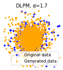
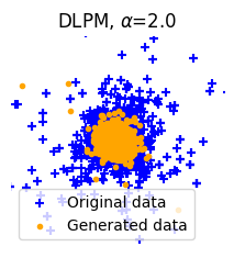
Figure 2: DLPM with $\alpha=1.7$ and $\alpha=2.$. The lighter tailed process fails to capture the distribution’s tail.

Enhancing data coverage: capturing the tail of the distribution.

We set $d=2$ and generate data points distributed as $\mathcal{S}^{\text{i}}_{\alpha}(0,0.05\cdot\mathrm{I}_{d})$, with $\alpha=1.7$. Our aim is to test the ability of each method to cover the dataset correctly; the main challenge is to correctly capture the tails.

As we can visually observe in Figure 2, the backward diffusion process in the Gaussian case cannot produce truly heavy-tailed data, mainly stemming from the fact that its variance is always finite. As expected, we see improvements when using noise with $\alpha<2$.

To quantify this behaviour, we utilize the mean square logarithmic error (MSLE) metric, which compares the relative error between the higher quantiles (i.e., the quantiles corresponding to the tail region that has probability $1-\xi$) of the true and the generated data distribution (see Section G.3 for detailed definitions). We observe in Table 1 how, as $\alpha$ gets smaller, one gets better tail approximation.

Furthermore, DLPM consistently outperforms LIM, indicating that the generation process benefits from the heavy-tailed denoising formulation, rather than the continuous-time one, in this setting.

Method	1.7	1.8	1.9	2.0
DLPM	0.071 ± 0.028	0.099 ± 0.044	0.132 ± 0.101	0.798 ± 0.601
LIM	0.267 ± 0.077	0.653 ± 0.413	2.444 ± 1.067	1.239 ± 0.240

Table 1: $\text{MSLE}_{\xi=0.95}\downarrow$ averaged over 20 runs

Enhancing data coverage: addressing mode collapse.

To assess the robustness of DLPM to mode collapse, we consider an unbalanced mixture of nine Gaussian distributions. We set their standard deviation to $0.05$ and arrange them in a grid-like pattern with equal spacing, in the square $[-1,1]^{2}$. Their mixture weights range from $.01$ to $.3$ . We use the $F_{1}^{\text{pr}}$ score (i.e., the harmonic mean of precision and recall, see Section G.3) to assess, in a single summary statistic, the quality and diversity in the generated data. As shown in Table 2, we are able to achieve improved scores by choosing a tail index $\alpha<2$ with DLPM. This is not necessarily the case for LIM, which is furthermore consistently outperformed. We also notice that using non-isotropic noise brings similar advantages, although less consistently, as it achieves good scores for $\alpha=1.8,1.9$, but does not perform as well with smaller $\alpha$. Finally, DLPM₅ shows its strengths with better performance over all the range of $\alpha$, though at the cost of 5 times the run time.

Figure 3: Gaussian grid

Method	$\alpha=1.7$	$\alpha=1.8$	$\alpha=1.9$	$\alpha=2.0$
DLPM	0.78 ± 0.04	0.75 ± 0.05	0.75 ± 0.04	0.71 ± 0.03
DLPM5	0.79 ± 0.03	0.77 ± 0.08	0.80 ± 0.05	0.69 ± 0.05
DLPM${}^{\text{ni}}$	0.71 ± 0.02	0.77 ± 0.05	0.77 ± 0.05	0.70 ± 0.04
LIM	0.72 ± 0.02	0.63 ± 0.05	0.62 ± 0.02	0.65 ± 0.02

Table 2: $F_{1}^{\text{pr}}\uparrow$ score, averaged over 30 runs

4.2 Experiments on image data

To fairly illustrate the differences between LIM and DLPM, we use the same improved DDPM neural network architecture, as designed by Nichol and Dhariwal (2021). The specific configuration for each dataset is carefully described in Section G.2. Our experiments are designed to compare deterministic and stochastic generation methods under varying conditions, with the aim of elucidating the performance characteristics inherent to our new approach.

Table 3: FID$\downarrow$ across different methods. We take 1000 sampling steps in the stochastic sampling methods (LIM and DLPM) and 25 steps in the deterministic sampling methods (LIM-ODE and DLIM).

MNIST	$\alpha=1.5$	$\alpha=1.7$	$\alpha=1.8$	$\alpha=1.9$	$\alpha=2.0$
LIM	4.075	5.171	6.812	11.202	11.693
DLPM${}^{\text{ni}}$	44.173	14.055	5.739	3.618	-
DLPM5	3.801	3.030	2.506	2.705	-
DLPM	5.392	2.938	2.930	3.237	3.632
LIM-ODE	45.717	68.153	85.090	113.196	29.04
DLIM5	14.959	51.582	59.841	76.033	-
DLIM5	3.373	2.931	3.440	4.314	-
DLIM	3.376	2.811	3.178	3.273	5.183
CIFAR10_LT
LIM	16.13	16.21	17.67	19.24	21.56
DLPM	16.10	18.00	19.94	20.21	21.07
LIM-ODE	30.170	65.788	84.559	101.704	32.00
DLIM	20.699	20.775	21.967	22.799	23.999

Convergence speed.

Consistent with existing literature (Song et al. (2020)), our findings as shown in Figure 4 confirm that deterministic generation outperforms its stochastic counterpart significantly, especially when fewer than 100 diffusion steps are used, on both MNIST and CIFAR10_LT. As the number of diffusion steps increases, both of these sampling methods produce similar results. This observation highlights that the advantages of the diffusion process do not primarily stem from increased randomness at sampling time. Instead, these heavy-tailed processes may define more appropriate vector field on which the noise is transported back to the original data distribution, which would lead to improved model performance (see Karras et al. (2022) for similar discussions on DDPM vs DDIM).

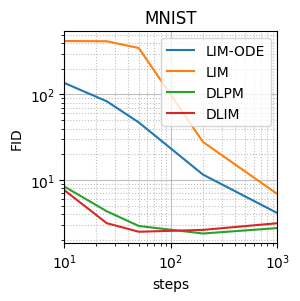
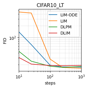
Figure 4: FID$\downarrow$ with varying step size, $\alpha=1.7$

The previous observations are quantitatively supported in Section 4.2, where we present results for both deterministic and stochastic sampling strategies. We compare both methods on stochastic generation at a high step count, to compare their performance at their best regime, and on deterministic generation at a small step count, to assess the tradeoff in computations/quality offered by both methods. As we can see, DLPM surpasses LIM on both datasets.

More interestingly, we observe in Section 4.2 that DLPM consistently outperforms LIM and offers satisfying image quality at low number of steps, both for stochastic and deterministic sampling. Generated images after $25$ steps achieve a FID score of $2.811$ on MNIST and of $20.699$ on CIFAR10_LT, as compared to respectively $45.717$ and $30.170$ for LIM-ODE. On MNIST, with $\alpha=1.7$, DLIM is able to match the sample quality of DLPM with 40 times less diffusion steps, further proving its efficacy. To visualize these behaviours, we display on Figure 5 different generation with varying time horizon $T$. We can see how the backward process defined by DLIM is able to approach the true data distribution more accurately.

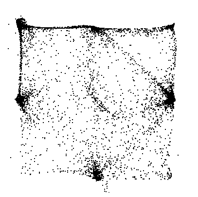
DLIM, 5 steps

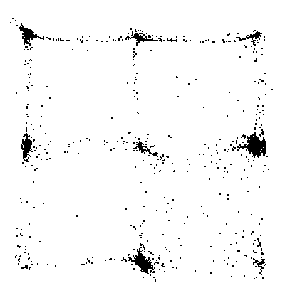
10 steps

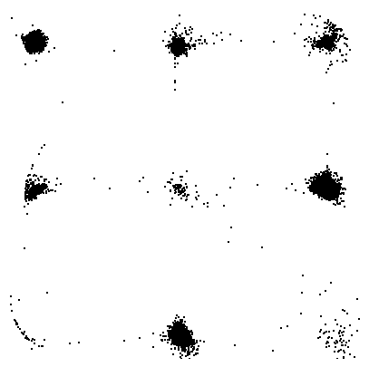
25 steps

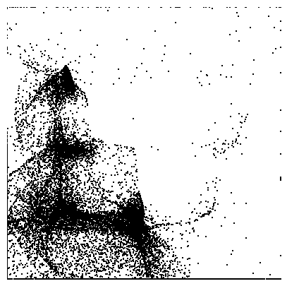
LIM, 5 steps

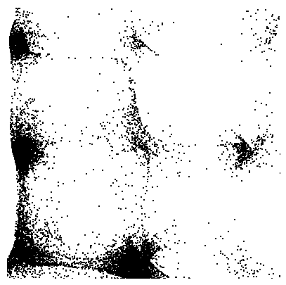
10 steps

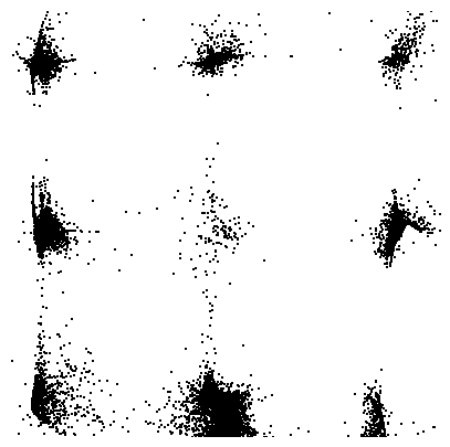
25 steps

Figure 5: DLIM and LIM-ODE with small number of steps, on the Gaussian grid of Figure 3.

Eventhough lower $\alpha$ usually entails lower FID in this table, LIM-ODE shows worse performance than the Gaussian diffusion at 25 reverse steps, except for $\alpha=1.5$; since the image quality is monotonically decreasing with $\alpha$ except for $\alpha=2$, we can conjecture that the initial instability introduced by heavy-tails are finally counterbalanced by the various benefits of heavy-tailed diffusion.

Finally, we mention our two other original additions. DLPM₅ shows consistent improvement over baseline, more particularly for stochastic sampling. DLPM${}^{\text{ni}}$ however shows worse performance, especially at smaller $\alpha$.

5 Conclusion

In this study, we proposed DLPM and DLIM, as heavy-tailed generalizations of DDPM and DDIM. As opposed to the state-of-the-art LIM method, our approach is based on elementary mathematical tools making it accessible to a broader audience and requires minor modifications to existing software implementations. The various experiments we have conducted suggest that DLPM is more effective in leveraging the characteristics of heavy-tailed distributions, providing robust performance across heavy-tailed data, unbalanced datasets and requiring a lower number of diffusion steps. Our experiments also illustrated that the efficiency of DLPM can be further improved by using our deterministic scheme DLIM.

Limitations and future work. The main limitation of our work is the additional computation burden stemming from the approximation of the expectations appearing in the loss function. As future work, we aim to circumvent this burden by directly estimating the $\mathrm{KL}$ divergence between two $\alpha$-stable vectors. Furthermore, we plan to investigate more advanced techniques, e.g,. as in elucidated diffusion models (Karras et al. (2022)), and explore the scalability of these methods and their efficacy across more diverse and complex datasets.

Broader impact. Compared to state-of-the-art, we believe that our approach would be more accessible to the community thanks to its simplicity. Hence, we believe our work might have positive societal impact and we do not foresee any direct negative societal impact.

Acknowledgments and Disclosure of Funding

A.D is funded by the European Union (ERC, Ocean, 101071601). D.S and U.S are partially funded by the European Union (ERC, Dynasty, 101039676). Views and opinions expressed are however those of the author(s) only and do not necessarily reflect those of the European Union or the European Research Council Executive Agency. Neither the European Union nor the granting authority can be held responsible for them.

U.S is additionally funded by the French government under management of Agence Nationale de la Recherche as part of the "Investissements d’avenir" program, reference ANR-19-P3IA-0001 (PRAIRIE 3IA Institute).

The authors are grateful to the CLEPS infrastructure from the Inria of Paris for providing resources and support.

Appendix

The Appendix is organized as follows:

• In Appendix A, we provide the pseudo-code for the training and sampling algorithms of DLPM and DLIM.

• In Appendix B, we characterize the stability property of the $\alpha$-stable distribution, and we give explicit formulas for the distribution of the sum of two $\alpha$-stable random variables.

• In Appendix C, we provide the detailed theory and derivations of the DLPM framework. Working on the process $\{X_{t}\}_{t=0}^{T}$ defined in (6), and its data augmentation counterpart $\{Y_{t}\}_{t=0}^{T}$ defined in (10), we start in Section C.2 by characterizing the distribution of $X_{t}$ given $X_{0}$ from a given noise schedule $\{(\gamma_{t},\sigma_{t})\}_{t=1}^{T}$, as this defines the characteristic location $\gamma_{1\to t}$ and scale $\sigma_{1\to t}$ of the process at time $t$. Likewise we characterize the distribution of $Y_{t}$ given $Y_{0},\{A_{t}\}_{t=1}^{T}$, as this defines the characteristic location $\gamma_{1\to t}$ and variance $\Sigma_{1\to t}$ of the augmented process at time $t$.

  In Section C.3, we focus on the Gaussian trick exploited by the process $\{Y_{t}\}_{t=0}^{T}$ defined in (10). This leads us to the an explicit formula for the Gaussian density of the backward process conditioned on a sequence $\{A_{t}\}_{t=1}^{T}$ of $\alpha$-stable random variables.

  In Section C.4, we further put this characterization into good use by obtaining a closed-form formula for the loss function . Follows a discussion on design choices for the model and the loss function at hand, which leads us to a simplified training loss (67) corresponding to the denoising loss for $\alpha$-stable diffusion.

  In Section C.5, we provide a faster sampling strategy for training DLPM, computing each loss term $\mathscr{L}^{\mathrm{L}}_{t-1}$ using only two heavy-tailed random variables per datapoint, instead of $t$ random variables.

  Finally we provide in Section C.5.1 a more principled approach to derive the loss function at hand.

• In Appendix D, we adapt the setting for deterministic sampling in classical denoising diffusion DDIM (Song et al. (2020)) to our $\alpha$-stable framework. We naturally call this extension DLIM. Alike DDIM, it is true that the same models can be used for both the DLIM and DLPM generation procedures.

• In Appendix E, we compare in more details the two discrete and continuous frameworks DLPM and LIM, underlining how they offer two distinct loss functions, training and sampling algorithms.

• In Appendix F, we give proofs relative to our technique for faster training, as introduced in Section C.5.

• In Appendix G, we provide additional experimental details.

Appendix A Algorithms for DLPM and DLIM

In this section, we explicitly provide the algorithms needed to train and sample from the DLPM and DLIM generative methods.

A.1 Training

The same models can be shared between DLPM and DLIM, as underlined in Section D.3. We introduce the values $\sigma_{1\to t},\gamma_{1\to t}$ determined by the noise schedule, as presented in Proposition 3:

$$\gamma_{1\to t}=\prod_{i=1}^{t}\gamma_{t}\;,\qquad\sigma_{1\to t}=\left[\sum_{i=1}^{t}\left(\frac{\gamma_{1\to t}}{\gamma_{1\to i}}\sigma_{i}\right)^{\alpha}\right]^{1/\alpha}\;.$$ (17)

Moreover we set $\gamma_{1\to 0}=\sigma_{1\to 0}=0$. We define $c_{A}=\cos^{2/\alpha}(\uppi\alpha/4)$ as in Theorem 1. We make the design choices D1, D2, D3 for our model, as described in Section C.4.2. Finally, we use the method for faster sampling as described in Section C.5. The resulting training algorithm is given in Algorithm 2.

Algorithm 1 Loss function for DLPM

1:model $\hat{\epsilon}^{\theta}_{t}$ noise schedule $\{(\gamma_{t},\sigma_{t})\}_{1\leqslant t\leqslant T}$, time $t\geqslant 1$, data $Y_{0}$

2:Sample $\bar{A}^{t}_{0},\bar{A}^{t}_{1}\sim\mathcal{S}_{\alpha/2,1}(0,c_{A})$

3:if $t=1$ then

4:     $\bar{A}^{t}_{0}=0$

5:end if

6:Sample $G_{t}\sim\mathcal{N}(0,\mathrm{I}_{d})$

7:$\Sigma^{\prime}_{t-1}(\bar{A}^{t}_{0})\leftarrow\bar{A}^{t}_{0}\sigma_{1\to t-1}^{2}$

8:$\Sigma^{\prime}_{t}(\bar{A}^{t}_{0,1})\leftarrow\bar{A}^{t}_{1}\sigma_{t}^{2}+\gamma_{t}^{2}\Sigma^{\prime}_{t-1}(\bar{A}^{t}_{0})$

9:$Y_{t}\leftarrow\gamma_{1\to t}Y_{0}+\Sigma^{\prime}_{t}(\bar{A}^{t}_{0,1})^{1/2}G_{t}$

10:$L_{t-1}\leftarrow\|\hat{\epsilon}^{\theta}_{t}(Y_{t})-\Sigma^{\prime}_{t}(\bar{A}^{t}_{0,1})^{1/2}G_{t}\|_{2}$ return $L_{t-1}$

Algorithm 2 DLPM training - simplified loss

A.2 Sampling

Given the noise schedule and a sequence $\{A_{t}\}_{t=1}^{T}$ of $\alpha$-stable random variables we define:

$$\Sigma_{1\to t}(A_{1:t})=\sum_{k=1}^{t}\left(\frac{\gamma_{1\to t}}{\gamma_{1\to k}}\sqrt{A_{k}}\sigma_{k}\right)^{2}\;,\quad\Gamma_{t}(A_{1:t})=1-\frac{\gamma_{t}^{2}\Sigma_{1\to t-1}(A_{1:t-1})}{\Sigma_{1\to t}(A_{1:t})}\;,$$ (18)

see Proposition 5 and Equation 25 from Proposition 4 for precise statements. We give our sampling algorithm for DLPM in Algorithm 3.

Algorithm 3 Stochastic sampling (DLPM)

1:model $\hat{\epsilon}^{\theta}_{t}$ noise schedule $\{(\gamma_{t},\sigma_{t})\}_{1\leqslant t\leqslant T}$

2:Sample $Y_{T}\sim\mathcal{S}(0,\sigma_{1\to T}\mathrm{I}_{d})$

3:Sample $\{A_{t}\}_{t=1}^{T}$ i.i.d.  $A_{t}\sim\mathcal{S}_{\alpha/2,1}(0,c_{A})$

4:for $t\leftarrow T\textrm{ to }1$ do

5:     Compute $\Sigma_{1\to t}(A_{1:t}),\Sigma_{1\to t-1}(A_{1:t-1}),\Gamma_{t}(A_{1:t})$ as in (18)

6:     Sample $G_{t}\sim\mathcal{N}(0,\mathrm{I}_{d})$

7:     $\hat{\Sigma}^{\theta}_{t-1}(A_{1:t})\leftarrow\Gamma_{t}(A_{1:t})\Sigma_{1\to t-1}(A_{1:t-1})$

8:     $Y_{t-1}\leftarrow Y_{t}/\gamma_{t}-{\Gamma_{t}(A_{1:t})\sigma_{1\to t}}\hat{\epsilon}^{\theta}_{t}(Y_{t})+\sqrt{\hat{\Sigma}^{\theta}_{t-1}(A_{1:t})}G_{t}$

9:end forreturn $Y_{0}$

For DLIM, one can potentially provide $Y_{T}$ as input, in order to use the support of the noise distribution as a latent space, alike what is done by Song et al. (2020). We give our DLIM sampling algorithm in Algorithm 4.

Algorithm 4 Deterministic sampling (DLIM)

1:model $\hat{\epsilon}^{\theta}_{t}$, noise schedule $\{(\gamma_{t},\sigma_{t})\}_{1\leqslant t\leqslant T}$

2:Sample $Y_{T}\sim\mathcal{S}^{\text{i}}_{\alpha}(0,\mathrm{I}_{d})$

3:for $t\leftarrow T\textrm{ to }1$ do

4:     $Y_{t-1}\leftarrow\dfrac{Y_{t}}{\gamma_{t}}-\left(\dfrac{\sigma_{1\to t}}{\gamma_{t}}-\sigma_{1\to t-1}\right)\hat{\epsilon}^{\theta}_{t}(Y_{t})$

5:end forreturn $Y_{0}$

Appendix B Additional Remark on $\alpha$-stable Distributions

Stable distributions are closed under convolution for a fixed value of $\alpha$. Since convolution is equivalent to multiplication of the Fourier-transformed function, it follows that the product of two stable characteristic functions with the same $\alpha$ will yield another such characteristic function. We precisely characterize this stability property in the following proposition:

Proposition 2 (See (Nolan, 2020, Proposition 1.3))

Let $X_{1},X_{2}$ be two random variables respectively distributed as $X_{1}\sim\mathcal{S}_{\alpha,\beta_{1}}(\mu_{1},\sigma_{1})$ and $X_{2}\sim\mathcal{S}_{\alpha,\beta_{2}}(\mu_{2},\sigma_{2})$, with $\mu_{1},\mu_{2},\beta_{1},\beta_{2}\in\mathbb{R}$ and $\sigma_{1},\sigma_{2}>0$. Then, $X=X_{1}+X_{2}$ is distributed as $\mathcal{S}_{\alpha,\beta}(\mu,\sigma)$ where:

$$\mu=\mu_{1}+\mu_{2}\;,\qquad\sigma=(\sigma_{1}^{\alpha}+\sigma_{2}^{\alpha})^{1/\alpha}\;,\qquad\beta=\dfrac{\beta_{1}\sigma_{1}^{\alpha}+\beta_{2}\sigma_{2}^{\alpha}}{\sigma_{1}^{\alpha}+\sigma_{2}^{\alpha}}\;.$$ (19)

In particular, when $X_{1},X_{2}$ are such that $X_{1}\sim\mathcal{S}_{\alpha}(0,\sigma_{1}),X_{2}\sim\mathcal{S}_{\alpha}(0,\sigma_{2})$, then $X=X_{1}+X_{2}\sim\mathcal{S}_{\alpha}(0,(\sigma_{1}^{\alpha}+\sigma_{2}^{\alpha})^{1/\alpha})$, which is the key relation used in the later characterizations of the distribution of our forward process.

Appendix C Theoretical properties of DLPM

In this section, we provide the detailed theory and associated derivations of the DLPM framework.

C.1 Setting and notations

We will denote by $\upphi_{d}(\cdot|\mu,\Sigma)$ the density of $\mathcal{N}(\mu,\Sigma)$, where $\mu\in\mathbb{R}^{d}$ and $\Sigma\in\mathbb{R}^{d\times d}$. We will denote by $\uppsi^{(\alpha)}$ the density of $\mathcal{S}_{\alpha/2,1}(0,c_{A})$, where $c_{A}=\cos^{2/\alpha}(\uppi\alpha/4)$.

Forward process.

We reintroduce the setting presented in Section 3, with the noising schedule being denoted by $\{(\gamma_{t},\sigma_{t})\}_{t=1}^{T}$, and the following forward process on which DLPM is based:

$$X_{0}\sim p_{\star}\;,\quad\text{ and }\quad X_{t}=\gamma_{t}X_{t-1}+\sigma_{t}\epsilon_{t}^{(\alpha)},$$ (20)

where $p_{\star}$ is the data distribution and $\{\epsilon^{(\alpha)}_{t}\}_{t=1}^{T}$ are independent random variables distributed as $\mathcal{S}^{\text{i}}_{\alpha}(0,\mathrm{I}_{d})$.

Data augmentation process.

We also introduce the associated data augmentation process:

$$Y_{0}\sim p_{\star}\;,\quad\text{ and }\quad Y_{t}=\gamma_{t}Y_{t-1}+\sigma_{t}A_{t}^{1/2}G_{t}\;,$$ (21)

where $\{G_{t}\}_{t=1}^{T}$ and $\{A_{t}\}_{t=1}^{T}$ are independent random variables distributed according to $G_{t}\sim\mathcal{N}(0,\mathrm{I}_{d})$ and $A_{t}\sim\mathcal{S}_{\alpha/2,1}(0,c_{A})$, with $c_{A}=\cos^{2/\alpha}(\uppi\alpha/4)$. From Theorem 1, $\{Y_{t}\}_{t=0}^{T}$ is a Markov chain that admits the same distribution as $\{X_{t}\}_{t=0}^{T}$. We will denote by $p_{t}^{(\alpha)}$ the distribution of $Y_{t}$, and by $k_{t|t-1}^{(\alpha)}(\cdot|\cdot)$ the transition density associated to the Markov chain (20).

Backward process.

A backward process associated to the Markov chain $\{Y_{t}\}_{t=0}^{T}$ is a Markov chain $\{\overleftarrow{Y^{\prime}}_{t}\}_{t=0}^{T}$ such that the two processes $\{\overleftarrow{Y^{\prime}}_{T-t}\}_{t=0}^{T}$ and $\{Y_{t}\}_{t=0}^{T}$ have the same distribution. For ease of presentation and following classical notations, we will rather consider $\{\overleftarrow{Y}_{t}\}_{t=0}^{T}$ where $\overleftarrow{Y}_{t}=\overleftarrow{Y^{\prime}}_{T-t}$. We will denote by $\overleftarrow{k}_{t-1|t}^{(\alpha)}(\cdot|\cdot)$ the transition densities associated to the process $\{\overleftarrow{Y}_{t}\}_{t=0}^{T}$. Since the true backward process is never available to us, we will focus on an approximation induced by a variational family. We consider the process $\{\overleftarrow{Y}^{\theta}_{t}\}_{t=0}^{T}$ where $\overleftarrow{Y}^{\theta}_{T}$ is distributed as $\mathcal{S}(0,\sigma_{1\to t}\mathrm{I}_{d})$, and the density of the distribution of $\overleftarrow{Y}^{\theta}_{t-1}$ conditioned on $\overleftarrow{Y}^{\theta}_{t}$ are given by $\overleftarrow{q}_{t-1|t}^{\theta}(\cdot|\cdot)$, where $\theta\in\mathbb{R}^{D}$ parameterizes a neural network. We also denote by $\overleftarrow{q}_{0:T}^{\theta}$ the joint distribution of $\{\overleftarrow{Y}^{\theta}\}_{t=0}^{T}$ and by $\overleftarrow{q}_{t}^{\theta}$ the marginal distribution of $\overleftarrow{Y}^{\theta}_{t}$.

Further notations.

Finally, we denote by $p_{t}^{\alpha}(\cdot|a_{1:t})$, $k_{t|t-1,a}^{(\alpha)}(\cdot|\cdot,a_{1:t})$, and $\overleftarrow{q}_{t-1|t,a}^{\theta}(\cdot|\cdot,a_{1:t})$ the densities/transition densities associated to the processes $\{Y_{t}\}_{t=0}^{T},\{\overleftarrow{Y}^{\theta}_{t}\}_{t=0}^{T}$ given $A_{t}=a_{t}$ for $1\leqslant t\leqslant T$. We we will also write $p_{t}^{\alpha}(\cdot|y_{0},a_{1:t})$, $k_{t|t-1,0,a}^{(\alpha)}(\cdot|\cdot,y_{0},a_{1:t})$, and $\overleftarrow{q}_{t-1|t,0,a}^{\theta}(\cdot|\cdot,y_{0},a_{1:t})$ when further conditioning on $Y_{0}$.

C.2 Forward process

Let us now characterize the distribution of $X_{t}$ given $X_{0}$, and $Y_{t}$ given $Y_{0},\{A_{t}\}_{t=1}^{T}$, which are tractable thanks to Proposition 2. These will come in handy, for instance when working on the backward process in Section C.3.

Proposition 3 (Distribution of $X_{t}$ given $X_{0}$)

Let $\{X_{t}\}_{t=0}^{T}$ be the forward process as given in (20), and $\{(\gamma_{t},\sigma_{t})\}_{t=1}^{T}$ the noise schedule. Then the distribution of $X_{t}$ given $X_{0}$ is given for any $t$ by

$$X_{t}\,{\buildrel d\over{=}}\,\gamma_{1\to t}X_{0}+\sigma_{1\to t}\bar{\epsilon}_{t}$$ (22)

where $\bar{\epsilon}_{t}\sim\mathcal{S}^{\text{i}}_{\alpha}(0,\mathrm{I}_{d})$, and $\gamma_{1\to t},\sigma_{1\to t}$ are given by:

$$\gamma_{1\to t}=\prod_{k=1}^{t}\gamma_{k}\;,\qquad\sigma_{1\to t}=\left(\sum_{k=1}^{t}\left(\dfrac{\gamma_{1\to t}}{\gamma_{1\to k}}\sigma_{k}\right)^{\alpha}\right)^{1/\alpha}\;.$$ (23)

The proof is an elementary induction based on Proposition 2.

Proposition 4 (Distribution of $Y_{t}$ given $Y_{0},\{A_{t}\}_{t=1}^{T}$)

Let $\{Y_{t}\}_{t=0}^{T}$ be the forward process as given in (21), $\{(\gamma_{t},\sigma_{t})\}_{t=1}^{T}$ the noise schedule, and $\{A_{t}\}_{t=1}^{T}$ the associated $\alpha/2$-stable random variables, parameterizing the variance of the Gaussian noise increments. Then the distribution of $Y_{t}$ given $Y_{0},\{A_{t}\}_{t=1}^{T}$ is the Gaussian distribution with mean $\gamma_{1\to t}Y_{0}$ and covariance matrix $\Sigma_{1\to t}\mathrm{I}_{d}$, i.e.,

$$Y_{t}\,{\buildrel d\over{=}}\,\gamma_{1\to t}Y_{0}+\Sigma_{1\to t}(A_{1:t})^{1/2}\bar{G}_{t}\;,$$ (24)

where $\bar{G}_{t}\sim\mathcal{N}(0,\mathrm{I}_{d})$, and

$$\gamma_{1\to t}=\prod_{k=1}^{t}\gamma_{k}\;,\qquad\Sigma_{1\to t}(A_{1:t})=\sum_{k=1}^{t}\left(\frac{\gamma_{1\to t}}{\gamma_{1\to k}}\sqrt{A_{k}}\sigma_{k}\right)^{2}\;.$$ (25)

The proof is elementary and omitted.

C.3 Backward process

Consider the setting of the data augmentation approach as given in (21). By the same arguments used in Section 3, it can be verified that a process starting from $p_{T}^{(\alpha)}$ and with transition densities $\overleftarrow{k}_{t-1|t}^{(\alpha)}(y_{t-1}|y_{t})\propto p_{t}^{(\alpha)}(y_{t-1})k_{t|t-1}^{(\alpha)}(y_{t}|y_{t-1})$ for any $y_{t-1},y_{t}$ is a backward process associated with $\{Y_{t}\}_{t=0}^{T}$. However, it raises two main problems. First (i), we cannot characterize the distribution of $\overleftarrow{k}_{t-1|t}^{(\alpha)}(y_{t-1}|y_{t})$, since we do not know the data distribution. Second (ii), in the case where $\alpha<2$, we do not have access to an explicit expression for $\overleftarrow{k}_{t-1|t,0}^{(\alpha)}(y_{t-1}|y_{t},y_{0})$.

Regarding (i), we have access to the distribution of $Y_{t}$ given $Y_{0}$, so a valid strategy consists in devising a method relying on characterizing the backward of the process $\{Y_{t}\}_{t=0}^{T}$ given $Y_{0}$. This is the classical strategy used in DDPM (Ho et al. (2020)), which is possible in the case $\alpha=2$ since $\overleftarrow{k}_{t-1|t,0}^{(\alpha)}(y_{t-1}|y_{t},y_{0})$ admits an analytical expression for any $y_{0},y_{t-1},y_{t}$, thanks to the properties of the Gaussian distribution.

Regarding (ii), in the case where $\alpha<2$, we make use of the trick introduced in Theorem 1, justifying the data augmentation approach. We will rather characterize the density of the Markov kernels associated to the backward of the process $\{Y_{t}\}_{t=0}^{T}$ given $Y_{0}$ and $\{A_{t}\}_{t=1}^{T}$. This time, since we manage Gaussian noise increments, we can fall back to the classical strategy, as we further develop in the following proposition.

Proposition 5 (Density of the backward process associated to $\{Y_{t}\}_{t=0}^{T}$ given $Y_{0},\{A_{t}\}_{t=1}^{T}$)

Consider the setting of the data augmentation approach as given in (21). Let $\{(\gamma_{t},\sigma_{t})\}_{t=1}^{T}$ be the noise schedule at hand. Let $k_{t-1|0,t,a}^{(\alpha)}(\cdot|y_{t},y_{0},a_{1:t})$ be the density of the backward process associated to $\{Y_{t}\}_{t=0}^{T}$ given $Y_{0}$ and $\{A_{t}\}_{t=1}^{T}$. Then $k_{t-1|t,0,a}^{(\alpha)}(\cdot|y_{t},y_{0},a_{1:t})$ is the density of a Gaussian distribution $\mathcal{N}(\tilde{\mathtt{m}}_{t-1},\tilde{\Sigma}_{t-1})$ with mean $\tilde{\mathtt{m}}_{t-1}$ and variance $\tilde{\Sigma}_{t-1}$ such that

$$\tilde{\mathtt{m}}_{t-1}(y_{t},y_{0},a_{1:t})=\frac{1}{\gamma_{t}}\left(y_{t}-\Gamma_{t}(a_{1:t})\sigma_{1\to t}\epsilon_{t}(y_{t},y_{0})\right)\;,\quad\tilde{\Sigma}_{t-1}(a_{1:t})=\Gamma_{t}(a_{1:t})\Sigma_{1\to t-1}(a_{1:t-1})\;,$$ (26)

where

$$\Sigma_{1\to t}(a_{1:t}) =\sum_{k=1}^{t}\left(\frac{\gamma_{1\to t}}{\gamma_{1\to k}}\sqrt{a_{k}}\sigma_{k}\right)^{2}$$ (27)

$$\epsilon_{t}(y_{t},y_{0}) =\frac{y_{t}-\gamma_{1\to t}y_{0}}{\sigma_{1\to t}}$$ (28)

$$\Gamma_{t}(a_{1:t}) =1-\frac{\gamma_{t}^{2}\Sigma_{1\to t-1}(a_{1:t-1})}{\Sigma_{1\to t}(a_{1:t})}\;.$$ (29)

Eventhough $\Gamma_{t}$ involves multiple heavy-tailed random variables, it is nonetheless bounded: $0\leqslant\Gamma_{t}\leqslant 1$.

Proof  To determine $k_{t-1|t,0,a}^{(\alpha)}(\cdot|y_{t},y_{0},a_{1:t})$, we need to work on the joint distribution of $(Y_{t-1},Y_{t})$ conditioned on $Y_{0},\{A_{t}\}_{t=1}^{T}$, which is a Gaussian vector for which classical techniques will let us derive the distribution of $Y_{t-1}$ given $Y_{t}$. Before doing so we need to compute $\rho_{t}$ the covariance of $Y_{t-1}$ and $Y_{t}$ given $Y_{0},\{A_{t}\}_{t=1}^{T}$, which we do thanks to Proposition 4:

$$\rho_{t}=\text{Cov}(Y_{t},Y_{t-1}|Y_{0},A_{1:T})=\gamma_{t}\text{Cov}(Y_{t-1},Y_{t-1}|Y_{0},A_{1:T})=\gamma_{t}\Sigma_{1\to t-1}\mathrm{I}_{d}.$$ (30)

Denote by $k_{t-1,t|0,a}^{(\alpha)}$ the density of $(Y_{t-1},Y_{t})$ conditioned on $Y_{0},A_{1:T}$. Denote by $\upphi_{d}(\cdot|\mu,\Sigma)$ the density of a $d$-dimensional Gaussian distribution with mean $\mu$ and covariance $\Sigma$. From the results of Proposition 4, we can write

$$k_{t-1,t|0,a}^{(\alpha)}(y_{t-1},y_{t}|y_{0},a_{1:t})=\upphi_{d}\left(\begin{pmatrix}y_{t-1}\\ y_{t}\end{pmatrix}\bigg{|}\begin{pmatrix}\gamma_{1\to t-1}y_{0}\\ \gamma_{1\to t}y_{0}\end{pmatrix},\begin{pmatrix}\Sigma_{1\to t-1}(a_{1:t-1})\mathrm{I}_{d}&\rho_{t}\mathrm{I}_{d}\\ \rho_{t}\mathrm{I}_{d}&\Sigma_{1\to t}(a_{1:t})\mathrm{I}_{d}\end{pmatrix}\right)$$ (31)

Then the distribution of $Y_{t-1}$ given $Y_{t},Y_{0},A_{1:T}$ is a Gaussian distribution $\mathcal{N}(\tilde{\mathtt{m}}_{t-1},\tilde{\Sigma}_{t-1})$ (Holt and Nguyen, 2023, Theorem 3) with mean $\tilde{\mathtt{m}}_{t-1}$ and variance $\tilde{\Sigma}_{t-1}$ satisfying:

$$\tilde{\mathtt{m}}_{t-1}(y_{t},y_{0},a_{1:t}) =\gamma_{1\to t-1}y_{0}+\dfrac{\rho_{t}}{\Sigma_{1\to t}(a_{1:t})}\left(y_{t}-\gamma_{1\to t}y_{0}\right)$$ (32)

$$\tilde{\Sigma}_{t-1}(a_{1:t}) =\Sigma_{1\to t-1}(a_{1:t-1})-\dfrac{\rho_{t}^{2}}{\Sigma_{1\to t}(a_{1:t})}\;.$$ (33)

By defining

$$\epsilon_{t}(y_{t},y_{0})=\frac{y_{t}-\gamma_{1\to t}y_{0}}{\sigma_{1\to t}}\;,\quad\Gamma_{t}(a_{1:t})=1-\frac{\gamma_{t}^{2}\Sigma_{1\to t-1}(a_{1:t-1})}{\Sigma_{1\to t}(a_{1:t})}\;,$$ (34)

we give the final expression for the mean $\tilde{\mathtt{m}}_{t-1}$ and variance $\tilde{\Sigma}_{t-1}$ of the distribution of $Y_{t-1}$ given $Y_{t},Y_{0}$ and $\{A_{t}\}_{t=1}^{T}$:

$$\tilde{\mathtt{m}}_{t-1}(y_{t},y_{0},a_{1:t}) =\dfrac{1}{\gamma_{t}}\left(y_{t}-\sigma_{1\to t}\Gamma_{t}(a_{1:t})\epsilon_{t}(y_{t},y_{0})\right)$$ (35)

$$\tilde{\Sigma}_{t-1}(a_{1:t}) =\Gamma_{t}(A_{1:t})\Sigma_{1\to t-1}(a_{1:t-1})\;.$$ (36)

Since $\Gamma_{t}(a_{1:t})=1-\gamma_{t}^{2}\Sigma_{1\to t-1}(a_{1:t-1})/\Sigma_{1\to t}(a_{1:t})=a_{t}\sigma_{t}^{2}/\Sigma_{1\to t}(a_{1:t})$ and $a_{t},\gamma_{t},\Sigma_{1\to t},\sigma_{1\to t}>0$, we have $0\leqslant\Gamma_{t}\leqslant 1$.

 

Case $\alpha=2$

As we set $\alpha=2$, the random variables $\{A_{t}\}_{t=1}^{T}$ become deterministic, equal to $2$. One can check that in this case, with the variance preserving schedule

$$\gamma_{t}=\sqrt{1-\beta_{t}}\;,\quad\gamma_{1\to t}=\sqrt{\alpha_{t}}\;,\quad\sigma_{t}=\sqrt{\beta_{t}}\;,\quad\sigma_{1\to t}=\sqrt{1-\alpha_{t}}\;,$$ (37)

then:

$$\Sigma_{1\to t}=2\sigma_{1\to t}^{2}\;=2(1-\alpha_{t})\;.$$ (38)

Further noticing that $\gamma_{t}=\gamma_{1\to t}/\gamma_{1\to t-1}$, one computes

$$\Gamma_{t} =1-\frac{\sigma_{1\to t-1}^{2}\alpha_{t}/\alpha_{t-1}}{\sigma_{1\to t}^{2}}$$ (39)

$$=1-\frac{(1-\alpha_{t-1})\alpha_{t}/\alpha_{t-1}}{1-\alpha_{t}}$$ (40)

$$=\dfrac{1-\alpha_{t}/\alpha_{t-1}}{1-\alpha_{t}}\;,$$ (41)

so that one recovers the famous equations made popular in the seminal DDPM paper (Ho et al., 2020, Equation 7):

$$\tilde{\mathtt{m}}_{t-1} =\dfrac{\sqrt{\alpha_{t-1}}}{\sqrt{\alpha_{t}}}\left(Y_{t}-\dfrac{1-\alpha_{t}/\alpha_{t-1}}{\sqrt{1-\alpha_{t}}}\epsilon_{t}(Y_{t},Y_{0})\right)$$ (42)

$$\tilde{\Sigma}_{t-1} =\left(1-\alpha_{t-1}\right)\dfrac{1-\alpha_{t}/\alpha_{t-1}}{1-\alpha_{t}}\;,$$ (43)

with $\epsilon_{t}(Y_{t},Y_{0})={(Y_{t}-\sqrt{\alpha_{t}}Y_{0})}/{\sqrt{1-\alpha_{t}}}$.

Model for the reverse process.

We propose approximating the backward process associated to $\{Y_{t}\}_{t=0}^{T}$, given $\{A_{t}\}_{t=1}^{T}$, adapting the DDPM approach. This time, for the backward process, we characterized the conditional density of $Y_{t-1}$ given $Y_{0},Y_{t}$ and $\{A_{t}\}_{t=1}^{T}$:

$$\overleftarrow{k}_{1:T|0,a}^{(\alpha)}(y_{1:T}|y_{0},a_{1:T}):=p_{T}^{(\alpha)}(y_{T})\prod\nolimits_{t=T}^{1}k_{t-1|0,t,a}^{(\alpha)}(y_{t-1}|y_{t},y_{0},a_{1:t})\;,$$ (44)

where $k_{t-1|0,t,a}^{(\alpha)}(\cdot|y_{t},y_{0},a_{1:t})$ is the tractable density of a Gaussian distribution, as we have just proved in Proposition 5. We similarly reconsider the family of Gaussian variational approximation introduced in (9), modified to account for an i.i.d. sequence $\{A_{t}\}_{t=1}^{T}$:

$$\overleftarrow{q}_{t-1|t,a}^{\theta}(y_{t-1}|y_{t},a_{1:t})=\upphi_{d}(y_{t-1}|\hat{\mathtt{m}}^{\theta}_{t-1}(y_{t},a_{1:t}),\hat{\Sigma}^{\theta}_{t-1}(y_{t},a_{1:t}))\;,$$ (45)

where $\upphi_{d}$ is the density of the multivariate Gaussian distribution, so that the overall model for the backward process is the following:

$$\overleftarrow{q}_{0:T}^{\theta}(y_{0:T})=\int\uppsi^{(\alpha)}_{1:T}(a_{1:T})p_{T}(y_{T})\prod\nolimits_{t=1}^{T}\overleftarrow{q}_{t-1|t,a}^{\theta}(y_{t-1}|y_{t},a_{1:t})\mathrm{d}a_{1:T}\;,$$ (46)

where $\uppsi^{(\alpha)}_{1:T}(a_{1:T})=\prod_{i=1}^{T}\uppsi^{(\alpha)}(a_{i})$.

C.4 Training Loss

In this section, we draw inspiration from DDPM (Ho et al. (2020)) to obtain a loss function admitting a closed-form formula. We further provide three design choices which lead to a simplified training loss, corresponding to the denoising loss for $\alpha$-stable diffusion.

C.4.1 Classical loss for DDPM, $\alpha=2$

We start by reviewing what is classically done for DDPM, i.e., the case $\alpha=2$. The variational approximation $\{\overleftarrow{q}_{0:T}^{\theta}\,:\,\theta\in\Theta\}$, for some parameter space $\Theta$, is designed to admit the same decomposition as $\overleftarrow{k}_{0:T}^{(2)}$, i.e., $\overleftarrow{q}_{0:T}^{\theta}(x_{0:T})=\overleftarrow{q}_{T}^{\theta}(x_{T})\prod_{t=T}^{1}\overleftarrow{q}_{t-1|t}^{\theta}(x_{t-1}|x_{t})$, where $\overleftarrow{q}_{T}^{\theta}$ is chosen to be the density of $\mathcal{S}^{\text{i}}_{\alpha}(0,\sigma_{1\to t}\mathrm{I}_{d})$ as an approximation of $p_{T}^{(\alpha)}$. Then, it is trained on a classical upper bound of the KL loss $\mathscr{L}^{\mathrm{D}}:\theta\mapsto\mathrm{KL}(p_{\star}\|\overleftarrow{q}_{0}^{\theta})$ between the true and the generated distribution, which is a form of evidence lower bound loss (Ho et al., 2020, Equation 5). Thus one resorts to optimize the following sum:

$$\mathscr{L}^{\mathrm{D}}(\theta)\leqslant\mathscr{L}^{\mathrm{D}}_{T}+\sum_{t=2}^{T}\mathscr{L}^{\mathrm{D}}_{t-1}(\theta)+\mathscr{L}^{\mathrm{D}}_{0}(\theta)+C$$ (47)

where $C$ is a constant that does not depend on $\theta$, and

$$\mathscr{L}^{\mathrm{D}}_{T} =\mathbb{E}\left[\mathrm{KL}\left(k_{T|0}^{(2)}(\cdot|X_{0})\ \|\ \upphi_{d}(\cdot|0,\sigma_{1\to T}\mathrm{I}_{d})\right)\right]$$ (48)

$$\mathscr{L}^{\mathrm{D}}_{0}(\theta) =-\mathbb{E}\left[\log\left(\overleftarrow{q}_{0|1}^{\theta}(X_{0}|X_{1})\right)\right]$$ (49)

$$\mathscr{L}^{\mathrm{D}}_{t-1}(\theta) =\mathbb{E}\left[\mathrm{KL}\left(k_{t-1|0,t}^{(2)}(\cdot|X_{0},X_{t})\ \|\ \overleftarrow{q}_{t-1|t}^{\theta}(\cdot|X_{t})\right)\right]\;,$$ (50)

where $\{X_{t}\}_{t=0}^{T}$ is the process defined in (20), and $k_{t-1|0,t}^{(2)}$ is the conditional density of $X_{t-1}$ given $X_{0},X_{t}$. We make the following classical remarks on the terms of this loss (Sohl-Dickstein et al. (2015), Yang et al. (2024)). The term $\mathscr{L}^{\mathrm{D}}_{T}$ does not depend on $\theta$ but only on the chosen time horizon for the forward process, that determines the final variance of the Gaussian distribution $\mathcal{N}(0,\sigma_{1\to T}\mathrm{I}_{d})$. It is neglected. The effect of optimizing the first term $\mathscr{L}^{\mathrm{D}}_{0}(\theta)$ is negligible too.

More importantly, for the term $\mathscr{L}^{\mathrm{D}}_{t-1}(\theta)$, when using Gaussian variational approximations, i.e., as

$$\overleftarrow{q}_{t-1|t}^{\theta}(x_{t-1}|x_{t})=\upphi_{d}\left(x_{t-1}|\hat{\mathtt{m}}^{\theta}_{t-1}(x_{t}),\hat{\Sigma}^{\theta}_{t-1}(x_{t})\right)\;,$$ (51)

where $(x,\mathtt{m},\Sigma)\mapsto\upphi_{d}(x|\mathtt{m},\Sigma)$ is the $d$-dimensional density of the Gaussian distribution with mean $\mathtt{m}$ and covariance matrix $\Sigma$, $\hat{\mathtt{m}}^{\theta}_{t-1},\hat{\Sigma}^{\theta}_{t-1}$ are some functions of $x_{t}$ parameterized by $\theta$, it turns out that $\mathscr{L}^{\mathrm{D}}_{t-1}$ admits a closed-form expression. For a fixed variance $\hat{\Sigma}^{\theta}_{t-1}=\tilde{\Sigma}_{t-1}$, with $\tilde{\Sigma}_{t-1}$ given in (42), one resorts to optimize a convenient $\mathbb{L}_{2}$ loss function:

$$\mathscr{L}^{\mathrm{D}}_{t-1}(\theta)=\lambda_{t}\|\tilde{\mathtt{m}}_{t-1}(x_{t},x_{0})-\hat{\mathtt{m}}^{\theta}_{t-1}(x_{t})\|^{2},$$ (52)

where $\lambda_{t},\tilde{\mathtt{m}}_{t}$ depend on the noise schedule $(\gamma_{t},\sigma_{t})$ and $x_{t},x_{0}$.

Unfortunately, as we mentioned in Section 3, this solution cannot be used as such to learn the backward transitions associated to $\{X_{t}\}_{t=0}^{T}$ for $\alpha<2$. The main issue that we face stems from the fact that the density of $\alpha$-stable distributions are in most cases unknown, in contrast to Gaussian distributions. As a result, the conditional density $x_{t-1},x_{0},x_{t}\mapsto k_{t-1|0,t}^{(\alpha)}(x_{t-1}|x_{0},x_{t})$ is unknown for $\alpha<2$, which prevents us to have an explicit expression for $\theta\mapsto\mathscr{L}^{\mathrm{D}}_{t-1}(\theta)$.

Moreover, the absence of a second order moment for $\alpha$-stable distributions challenges the most straightforward adaptation we can make to the previous loss considering the data augmentation setting. Indeed, to fit $\theta$ to the data distribution, we aim to rely on Kullback-Leibler minimization, a.k.a. the maximum likelihood principle, and some associated upper bounds. A naive solution would consist in considering the bounds obtained applying the Jensen inequality:

$$\textstyle\mathrm{KL}(p_{\star}\|\overleftarrow{q}_{0}^{\theta})\leqslant\mathbb{E}\left[\mathrm{KL}\left[p_{\star}(\cdot)\|\overleftarrow{q}_{0|a}^{\theta}(\cdot|A_{1:T})\right]\right]\;,$$ (53)

and fall back to the expression obtained in (47), only with conditioning on $\{A_{t}\}_{t=1}^{T}$. However, as we see in (52), this expression would involve taking expectation of $A_{t}$, while it is distributed as $\mathcal{S}_{\alpha/2,1}(0,c_{A})$ and admits no first order moment. We are not aware of any bounds on $\mathrm{KL}(p_{\star}\parallel\overleftarrow{q}_{0|a}^{\theta}(\cdot|A_{1:T}))$ that would lead to a meaningful optimization problem due to the heavy tailed nature of the distribution of $\{A_{t}\}_{t=1}^{T}$.

C.4.2 Loss for DLPM, for any $\alpha$

We now expose our methodology to address this limitation. We keep the structure of the classical loss and aim at minimizing the error between the backward process $\{\overleftarrow{Y}_{t}\}_{t=0}^{T}$ and its variational approximation $\{\overleftarrow{Y}^{\theta}_{t}\}_{t=0}^{T}$. To do so we consider the same loss structure as before, but take the square root of individual KL terms. See Section C.5.1 for a more principled approach leading to a similar loss. Thus we consider the following valid loss function:

$$\mathscr{L}^{\mathrm{L}}:\theta\mapsto\mathscr{L}^{\mathrm{L}}(\theta)=\mathbb{E}\left[\sum_{t=2}^{T}\left(\mathscr{L}^{\mathrm{L}}_{t-1}(\theta,A_{1:t})\right)^{1/2}\right]\;,$$ (54)

where

$$\mathscr{L}^{\mathrm{L}}_{t-1}(\theta,A_{1:t})=\mathbb{E}\left[\mathrm{KL}\left(k_{t-1|t,0,a}^{(\alpha)}(\cdot|Y_{t},Y_{0},A_{1:t})\ \|\ \overleftarrow{q}_{t-1|t,a}^{\theta}(\cdot|Y_{t},A_{1:t})\right)\ \bigg{|}\ A_{1:t}\right]\;,$$ (55)

and $k_{t-1|0,t,a}^{(\alpha)}$ denotes the conditional density of $Y_{t-1}$ given $Y_{0},Y_{t}$ and $\{A_{t}\}_{t=1}^{T}$.

Proposition 6 (Training loss for DLPM)

The loss $\mathscr{L}^{\mathrm{L}}$ admits a closed-form expression, such that one resorts to optimize the following loss for $1\leqslant t\leqslant T$:

$$\mathscr{L}^{\mathrm{L}}_{t-1}(\theta,A_{1:t})=\mathbb{E}\bigg{[}\frac{1}{2}\log\dfrac{\hat{\Sigma}^{\theta}_{t-1}}{\tilde{\Sigma}_{t-1}}+\dfrac{\tilde{\Sigma}_{t-1}+\|\tilde{\mathtt{m}}_{t-1}-\hat{\mathtt{m}}^{\theta}_{t-1}\|^{2}}{2\hat{\Sigma}^{\theta}_{t-1}}-\dfrac{1}{2}\ \bigg{|}\ A_{1:t}\bigg{]}$$ (56)

where

$$\tilde{\mathtt{m}}_{t-1}(Y_{t},Y_{0},A_{1:t}) =\frac{1}{\gamma_{t}}\left(Y_{t}-\sigma_{1\to t}\Gamma_{t}(A_{1:t})\epsilon_{t}(Y_{t},Y_{0})\right)$$ (57)

$$\tilde{\Sigma}_{t-1}(A_{1:t}) =\Gamma_{t}(A_{1:t})\Sigma_{1\to t-1}(A_{1:t-1})$$ (58)

$$\epsilon_{t}(Y_{t},Y_{0}) =\frac{Y_{t}-\gamma_{1\to t}Y_{0}}{\sigma_{1\to t}}$$ (59)

$$\Sigma_{1\to t}(A_{1:t}) =\sum_{k=1}^{t}\left(\frac{\gamma_{1\to t}}{\gamma_{1\to k}}\sqrt{A_{k}}\sigma_{k}\right)^{2}$$ (60)

$$\Gamma_{t}(A_{1:t}) =1-\frac{\gamma_{t}^{2}\Sigma_{1\to t-1}(A_{1:t-1})}{\Sigma_{1\to t}(A_{1:t})}\;,$$ (61)

where $\hat{\mathtt{m}}^{\theta}_{t-1},\hat{\Sigma}^{\theta}_{t-1}$ are the mean and variance of the backward transition kernels $\overleftarrow{q}_{t-1|t}^{\theta}$. We have omitted the arguments of the mean and variance functions for clarity.

Proof  Recall (Proposition 5) that the backward process $Y_{t-1}$ conditioned on $\{A_{t}\}_{t=1}^{T},Y_{t},Y_{0}$ at time $t$ is distributed as $\mathcal{N}(\tilde{\mathtt{m}}_{t-1},\tilde{\Sigma}_{t-1})$, and, by design (Section 3), the backward transition kernels $\overleftarrow{q}_{t-1|t,a}^{\theta}$ of each element of the variational family describe a Gaussian transition kernel of mean $\hat{\mathtt{m}}^{\theta}_{t-1}$ and variance $\hat{\Sigma}^{\theta}_{t-1}$ at time $t$, as defined in 35. Since the KL term in $\mathscr{L}^{\mathrm{L}}_{t-1}(\theta,A_{1:t})$ corresponds to a KL divergence between two Gaussian distributions, a closed-form formula is readily available. Here we rewrite the equation with all the functions arguments written out explicitly:

$$\mathscr{L}^{\mathrm{L}}_{t-1}(\theta,A_{1:t})=\mathbb{E}\bigg{[} \frac{1}{2}\log\dfrac{\hat{\Sigma}^{\theta}_{t-1}(A_{1:t})}{\tilde{\Sigma}_{t-1}(A_{1:t})}-\dfrac{1}{2}$$ (62)

$$+\dfrac{\tilde{\Sigma}_{t-1}(A_{1:t})+\|\tilde{\mathtt{m}}_{t-1}(Y_{t},Y_{0},A_{1:t})-\hat{\mathtt{m}}^{\theta}_{t-1}(Y_{t},A_{1:t})\|^{2}}{2\hat{\Sigma}^{\theta}_{t-1}(A_{1:t})}\ \bigg{|}\ A_{1:t}\bigg{]}$$ (63)

 

Now we discuss further design choices for $\mathscr{L}^{\mathrm{L}}_{t-1}(\theta,A_{1:t})$, $\overleftarrow{q}_{t-1|t,a}^{\theta}$, leading to a simplified denoising loss, as is usually done in the literature. We denote them by D1, D2 and D3.

D1.

We set a fixed variance $\hat{\Sigma}^{\theta}_{t}=\tilde{\Sigma}_{t}$ for the reverse process , but we expect a study on the effect of learning variance to yield similar results as in original DDPM (Ho et al. (2020)), and especially its improved version (Nichol and Dhariwal (2021)).

D2.

Following our own experimental results and the usual recommendation for denoising diffusion models (see, e.g., Yang et al. (2024); Karras et al. (2022)), we reparameterize the output of the model to predict the value $\epsilon_{t}(y_{t},y_{0})$ at time-step $t$ rather than $\tilde{\mathtt{m}}_{t-1}(y_{t},y_{0},a_{1:t})$. Since

$$\tilde{\mathtt{m}}_{t-1}(Y_{t},Y_{0},A_{1:t})=\frac{1}{\gamma_{t}}\left(Y_{t}-\sigma_{1\to t}\Gamma_{t}(A_{1:t})\epsilon_{t}(Y_{t},Y_{0})\right)\;,$$ (64)

we re-parameterize $\hat{\mathtt{m}}^{\theta}_{t-1}$ to be equal to

$$\hat{\mathtt{m}}^{\theta}_{t-1}(Y_{t},A_{1:t})=\frac{1}{\gamma_{t}}\left(Y_{t}-\sigma_{1\to t}\Gamma_{t}(A_{1:t})\hat{\epsilon}^{\theta}_{t}(Y_{t},A_{1:t})\right)\;.$$ (65)

with $\hat{\epsilon}^{\theta}_{t}$ being the output of the model. Assuming D1, $\mathscr{L}^{\mathrm{L}}_{t-1}(\theta)$ becomes

$$\mathscr{L}^{\mathrm{L}}_{t-1}(\theta)=\mathbb{E}\left[\lambda_{t,\Gamma_{t}}^{2}\|\hat{\epsilon}^{\theta}_{t}(Y_{t},A_{1:t})-\epsilon_{t}(Y_{t},Y_{0})\|^{2}\right]\;,$$ (66)

where $\lambda_{t,\Gamma_{t}}={\Gamma_{t}\sigma_{1\to t}}/{2\gamma_{t}\tilde{\Sigma}}$, and $\epsilon_{t}(Y_{t},Y_{0})={(Y_{t}-\gamma_{1\to t}Y_{0})}/{\sigma_{1\to t}}$. At this point, the methodological knowledge of diffusion models could motivate us to make specific choices for $\lambda$ different from its exact definition, which is a classical technique for improving performances (e.g., see Karras et al. (2022); Ho et al. (2020); Nichol and Dhariwal (2021); Yang et al. (2024)). We will stick to the classical choice of choosing $\lambda=1$, which experimentally works well and draws similarities to the score-based perspective (Yoon et al. (2023)). Other choices and optimizations are left to further work.

D3.

Following experimental results (see the introduction of Appendix G), we drop the dependency of $\hat{\epsilon}^{\theta}_{t}$ on $\{A_{t}\}_{t=1}^{T}$, which is natural since it is supposed to approximate $\epsilon_{t}:(Y_{t},Y_{0})\mapsto\epsilon_{t}(Y_{t},Y_{0})$. Thus $\hat{\epsilon}^{\theta}_{t}$ only depends on $t,Y_{t}$. This choice achieves better performance in our experiments, allows further tricks (see Section C.5), and enables one to re-use existing neural network architectures.

Proposition 7 (Simplified denoising loss)

With the design choices D1, D2, D3, we obtain the simplified denoising objective function:

$$\mathscr{L}^{\mathrm{Simple}}(\theta)=\sum_{t=1}^{T}\mathbb{E}\left[\mathbb{E}\left(\|\hat{\epsilon}^{\theta}_{t}(Y_{t})-\epsilon_{t}(Y_{t},Y_{0})\|^{2}\ \big{|}\ A_{1:t}\right)^{1/2}\right]\;,$$ (67)

where the model $\hat{\epsilon}^{\theta}_{t}$ is designed to fit the noise $\epsilon_{t}(Y_{t},Y_{0})={(Y_{t}-\gamma_{1\to t}Y_{0})}/{\sigma_{1\to t}}={\Sigma_{1\to t}^{1/2}}/{\sigma_{1\to t}}G_{t}$ added at time-step $t$, and $\sigma_{1\to t},\Sigma_{1\to t}$ are as introduced in Proposition 3 and Proposition 4.

C.5 Reducing the computational cost with faster sampling at timestep t

In this section, we provide a faster algorithm for training DLPM, computing each loss term $\mathscr{L}^{\mathrm{L}}_{t-1}$ using only two heavy-tailed random variables per datapoint, instead of $t$ random variables.

Consider again the process $\{Y_{t}\}_{t=0}^{T}$. We replace the loss function (54) by an equivalent one:

$$\mathscr{L}^{\mathrm{L}}_{\text{time}}(\theta)=\mathbb{E}\left[\mathscr{L}^{\mathrm{L}}_{t-1}(\theta,A_{1:t})^{1/2}\right]\;,$$ (68)

where $t\sim\mathcal{U}[2,T]=(\sum_{i=2}^{T}\delta_{i})/(T-1)$. The standard technique for computing the loss consists in the following loop:

1. Take a batch of $B$ datapoints $\{Y_{0}^{i}\}_{i=1}^{B}$.

2. For each datapoint $Y_{0}^{i}$, draw a random $t_{i}$,as suggested by the alternative loss (68). Indeed, for a single datapoint, (i) training on all timesteps rather than just one yields equal to inferior results, for a much higher computational cost, (ii) it is beneficial for the model to proportionally spend more time learning specific time ranges (iii) thus the distribution of $t$ can be optimized and is a matter of ongoing methodological research, e.g., see Karras et al. (2022).

3. Draw sequences $\{A_{t}^{i}\}_{t=1}^{t_{i}}$ of heavy-tailed random variables.

4. Compute the noised datapoints $\{Y_{t_{i}}^{i}\}_{i=1}^{B}$.

5. Compute the batch loss

   $$\hat{\mathscr{L}}^{\mathrm{L}}(\theta)=\frac{1}{B}\sum_{i=1}^{B}\mathscr{L}^{\mathrm{L}}_{t_{i}-1}(\theta,Y_{t_{i}}^{i},A_{1:t_{i}}^{i})\;,$$ (69)

   such that $\hat{\mathscr{L}}^{\mathrm{L}}(\theta)\approx\mathscr{L}^{\mathrm{L}}_{\text{time}}(\theta)$.

6. Do an optimization step.

Step $3$ can be expensive, since one has to sample on average $O(T)$ $d$-dimensional heavy-tailed random variables to compute a single noised datapoint $Y_{t}$ from $Y_{0}$. This is all the more inefficient as $T$ can be quite large (indeed, on image datasets we can have $T=4000$, see Appendix G).

One can guess that this is abusive, especially since characterizing the distribution of $Y_{t}$ given $Y_{0}$ only requires a single heavy-tailed random variable:

$$Y_{t}\,{\buildrel d\over{=}}\,\gamma_{1\to t}Y_{0}+\sigma_{1\to t}\bar{A}^{1/2}\bar{G}_{t}\;,$$ (70)

where $\bar{A}\sim\mathcal{S}_{\alpha/2,1}(0,c_{A})$, $\bar{G}_{t}\sim\mathcal{N}(0,\mathrm{I}_{d})$. As we formalize in the next proposition, it is indeed possible to bypass the sampling of a whole sequence. Since we manipulate the joint distribution of $(Y_{0},Y_{t-1},Y_{t})$ for the loss term $\mathscr{L}^{\mathrm{L}}_{t-1}(\theta)$, we will actually need to sample two heavy-tailed random variables.

Proposition 8 (Sampling two heavy-tailed r.v for each loss term)

Suppose that the functions $\hat{\mathtt{m}}^{\theta}_{t-1},\hat{\Sigma}^{\theta}_{t-1}$ satisfy for any $y_{t},a_{1:t}$:

$$\hat{\mathtt{m}}^{\theta}_{t-1}(y_{t},a_{1:t}) =M^{\theta}_{t-1}\left(y_{t},a_{t},\frac{\Sigma_{1\to t-1}(a_{1:t-1})}{\sigma_{1\to t-1}^{2}}\right)$$ (71)

$$\hat{\Sigma}^{\theta}_{t-1} =S^{\theta}_{t-1}\left(y_{t},a_{t},\frac{\Sigma_{1\to t-1}(a_{1:t-1})}{\sigma_{1\to t-1}^{2}}\right)\;,$$ (72)

for some functions $M^{\theta}_{t-1},S^{\theta}_{t-1}$, and where

$$\Sigma_{1\to t}(a_{1:t})=\sum_{k=1}^{t}\left(\frac{\gamma_{1\to t}}{\gamma_{1\to k}}\sqrt{a_{k}}\sigma_{k}\right)^{2}\;,$$ (73)

as given in (25). Then each term $\mathbb{E}[\mathscr{L}^{\mathrm{L}}_{t-1}(\theta,A_{1:t})]^{1/2}$ of the loss can be computed sampling only two independent random variables $\bar{A}^{t}_{0},\bar{A}^{t}_{1}$ distributed as $\mathcal{S}_{\alpha/2,1}(0,c_{A})$:

$$\mathbb{E}\left[\mathscr{L}^{\mathrm{L}}_{t-1}(\theta,A_{1:t})\right]^{1/2}=\mathbb{E}\left[\mathscr{L}^{\mathrm{Less}}_{t-1}(\theta,\bar{A}^{t}_{0,1})\right]^{1/2}\;,$$ (74)

where $\bar{A}^{t}_{0,1}:=(\bar{A}^{t}_{0},\bar{A}^{t}_{1})$, and

$$\mathscr{L}^{\mathrm{Less}}_{t-1}(\theta,\bar{A}^{t}_{0,1})=\mathbb{E}\bigg{[} \frac{1}{2}\log\dfrac{S^{\theta}_{t-1}(Z_{t},\bar{A}^{t}_{0,1})}{\tilde{\Sigma}_{t-1}(\bar{A}^{t}_{0,1})}-\dfrac{1}{2}$$ (75)

$$+\dfrac{\tilde{\Sigma}_{t-1}(\bar{A}^{t}_{0,1})+\|\tilde{\mathtt{m}}_{t-1}^{\prime}(Z_{t},Z_{0},\bar{A}^{t}_{0,1})-M^{\theta}_{t-1}(Z_{t},\bar{A}^{t}_{0,1})\|^{2}}{2S^{\theta}_{t-1}(Z_{t},\bar{A}^{t}_{0,1})}\ \bigg{|}\ \bar{A}^{t}_{0,1}\bigg{]}\;,$$ (76)

with $\{Z_{t}\}_{t=0}^{T}$ being a stochastic process defined as

$$Z_{0}=Y_{0}\;,\quad Z_{t}=\gamma_{1\to t}Z_{0}+\Sigma_{t}^{\prime 1/2}G_{t}\;,$$ (77)

where

$$\Sigma^{\prime}_{t-1}(\bar{A}^{t}_{0}) =\sigma_{1\to t-1}^{2}\bar{A}^{t}_{0}$$ (78)

$$\Sigma^{\prime}_{t}(\bar{A}^{t}_{0,1}) =\sigma_{t}^{2}\bar{A}^{t}_{1}+\gamma_{t}^{2}\Sigma^{\prime}_{t-1}(\bar{A}^{t}_{0})$$ (79)

$$\Gamma^{\prime}_{t}(\bar{A}^{t}_{0,1}) =1-\dfrac{\gamma_{t}^{2}\Sigma^{\prime}_{t-1}(\bar{A}^{t}_{0})}{\Sigma^{\prime}_{t}(\bar{A}^{t}_{0,1})}\;,$$ (80)

such that $Z_{t}\,{\buildrel d\over{=}}\,Y_{t}$, and:

$$\tilde{\mathtt{m}}_{t-1}(Z_{t},Z_{0},\bar{A}^{t}_{0,1}) =\frac{1}{\gamma_{t}}\left(Z_{t}-\sigma_{1\to t}\Gamma^{\prime}_{t}(\bar{A}^{t}_{0,1})\epsilon_{t}(Z_{t},Z_{0})\right)$$ (81)

$$\tilde{\Sigma}_{t-1}(\bar{A}^{t}_{0,1}) =\Gamma^{\prime}_{t}(\bar{A}^{t}_{0,1})\Sigma^{\prime}_{t-1}(\bar{A}^{t}_{0})$$ (82)

$$\epsilon_{t}(Z_{t},Z_{0}) =\frac{Z_{t}-\gamma_{1\to t}Z_{0}}{\sigma_{1\to t}}\;.$$ (83)

In order to keep the notations similar for all $t\geqslant 2$, in the case of $\mathscr{L}^{\mathrm{Less}}_{1}$, we always set $\bar{A}^{2}_{0}=0$.

Proof  Remember the full equation for the loss, first given in Proposition 6 (62):

$$\mathscr{L}^{\mathrm{L}}_{t-1}(\theta,A_{1:t})=\mathbb{E}\bigg{[} \frac{1}{2}\log\dfrac{\hat{\Sigma}^{\theta}_{t-1}(A_{1:t})}{\tilde{\Sigma}_{t-1}(A_{1:t})}-\dfrac{1}{2}$$ (84)

$$+\dfrac{\tilde{\Sigma}_{t-1}(A_{1:T})+\|\tilde{\mathtt{m}}_{t-1}(Y_{t},Y_{0},A_{1:T})-\hat{\mathtt{m}}^{\theta}_{t-1}(Y_{t},A_{1:T})\|^{2}}{2\hat{\Sigma}^{\theta}_{t-1}(A_{1:t})}\ \bigg{|}\ A_{1:t}\bigg{]}\;.$$ (85)

Now, all the required variables and computations only depend on $A_{t},\Sigma_{1\to t-1}$; this is the case for $\hat{\mathtt{m}}^{\theta}_{t-1},\hat{\Sigma}^{\theta}_{t-1}$ by hypothesis, and this is the case for $\tilde{\mathtt{m}}_{t-1},\tilde{\Sigma}_{t-1}$ as one can see in (26). Rewriting the previous loss as

$$\mathscr{L}^{\mathrm{L}}_{t-1}(\theta,A_{1:t})=\mathbb{E}\bigg{[} \frac{1}{2}\log\dfrac{S^{\theta}_{t-1}\left(Z_{t},A_{t},\frac{\Sigma_{1\to t-1}(A_{1:t-1})}{\sigma_{1\to t-1}^{2}}\right)}{\tilde{\Sigma}_{t-1}(A_{1:T})}-\dfrac{1}{2}$$ (86)

$$+\dfrac{\tilde{\Sigma}_{t-1}(A_{1:t})}{2S^{\theta}_{t-1}\left(Z_{t},A_{t},\frac{\Sigma_{1\to t-1}(A_{1:t-1})}{\sigma_{1\to t-1}^{2}}\right)}$$ (87)

$$+\dfrac{\|\tilde{\mathtt{m}}_{t-1}(Y_{t},Y_{0},A_{1:t})-M^{\theta}_{t-1}\left(Z_{t},A_{t},\frac{\Sigma_{1\to t-1}(A_{1:t-1})}{\sigma_{1\to t-1}^{2}}\right)\|^{2}}{2S^{\theta}_{t-1}\left(Z_{t},A_{t},\frac{\Sigma_{1\to t-1}(A_{1:t-1})}{\sigma_{1\to t-1}^{2}}\right)}\ \bigg{|}\ A_{t},\Sigma_{1\to t-1}\bigg{]}\;,$$ (88)

it becomes clear how the expectation can be taken on the joint distribution of

$$\left(Y_{0},Y_{t-1},Y_{t},A_{t},\frac{\Sigma_{1\to t-1}(A_{1:t-1})}{\sigma_{1\to t-1}^{2}}\right)\;.$$ (89)

A direct application of Lemma 11 shows that this expectation can be taken on the joint distribution of the five random variables $(Z_{0},Z_{t-1},Z_{t},\bar{A}^{t}_{1},\bar{A}^{t}_{0})$, which only necessitates sampling two heavy-tailed random variables $\bar{A}^{t}_{0},\bar{A}^{t}_{1}$. Using the formulas for $Z_{0},Z_{t-1}$ and $Z_{t}$ given $\bar{A}^{t}_{0},\bar{A}^{t}_{1}$ as defined in Lemma 11, we obtain the equivalent loss (75).

 

With these choices, we can also rewrite the simplified denoising loss given in (67).

Proposition 9 (Sampling two heavy-tailed r.v in the simplified loss)

Consider the setting of Proposition 7 and the design choices D1, D2, D3. Then one can obtain the following simplified denoising objective function from the full objective function given in (75):

$$\mathscr{L}^{\mathrm{SimpleLess}}(\theta)=\sum_{t=1}^{T}\mathbb{E}\left[\mathbb{E}\left(\|\hat{\epsilon}^{\theta}_{t}(Z_{t})-\epsilon_{t}(Z_{t},Z_{0})\|^{2}\ |\ \bar{A}^{t}_{0},\bar{A}^{t}_{1}\right)\right]^{1/2},$$ (90)

where

$$Z_{t}=\gamma_{1\to t}Z_{0}+\Sigma_{t}^{\prime 1/2}G_{t}\;,\quad\epsilon_{t}(Z_{t},Z_{0})=\frac{Z_{t}-\gamma_{1\to t}Z_{0}}{\sigma_{1\to t}}\;,$$ (91)

and

$$\hat{\mathtt{m}}^{\theta}_{t-1}(Z_{t},\bar{A}^{t}_{0,1}) =\frac{1}{\gamma_{t}}\left(Z_{t}-\sigma_{1\to t}\Gamma^{\prime}_{t}(\bar{A}^{t}_{0,1})\hat{\epsilon}^{\theta}_{t}(Z_{t})\right)$$ (92)

$$\hat{\Sigma}^{\theta}_{t-1} =\Gamma^{\prime}_{t}(\bar{A}^{t}_{0,1})\Sigma^{\prime}_{t-1}(\bar{A}^{t}_{0})\;,$$ (93)

with

$$\Sigma^{\prime}_{t-1}(\bar{A}^{t}_{0})=\sigma_{1\to t-1}^{2}\bar{A}^{t}_{0},\quad\Sigma^{\prime}_{t}(\bar{A}^{t}_{0,1})=\sigma_{t}^{2}\bar{A}^{t}_{1}+\gamma_{t}^{2}\Sigma^{\prime}_{t-1}(\bar{A}^{t}_{0}),\quad\Gamma^{\prime}_{t}(\bar{A}^{t}_{0,1})=1-\dfrac{\gamma_{t}^{2}\Sigma^{\prime}_{t-1}(\bar{A}^{t}_{0})}{\Sigma^{\prime}_{t}(\bar{A}^{t}_{0,1})}\;.$$ (94)

We stress that this denoising training loss is similar to that of LIM (Yoon et al., 2023, Theorem 4.3), but with a necessary square root to guarantee that the loss is finite. See Section E.1 for a more detailed discussion.

C.5.1 A principled approach for deriving the loss function

In this section, we provide a more principled approach to derive the loss function for DLPM, as initially given in (54).

Noting that $Y_{0}$ is independent of $\{A_{t}\}_{t=1}^{T}$ in (10), $p_{\star}$ is the equal to $k_{0|a}^{(\alpha)}(\cdot|a_{1:T})$, the conditional density of $Y_{0}$ given $A_{t}=a_{t}$ for any $t\in\{1,\ldots,T\}$, and therefore, we consider the valid loss function

$$\mathscr{L}^{\mathrm{L}}(\theta):\theta\mapsto\int\mathrm{d}a_{1:T}\uppsi^{(\alpha)}_{1:T}(a_{1:T})\left[\mathrm{KL}(k_{0|a}^{(\alpha)}(\cdot|a_{1:T})\|\overleftarrow{q}_{0|a}^{\theta}(\cdot|a_{1:T}))\right]^{1/2}\;.$$ (95)

While this function is still intractable, we can provide an upper bound which we can minimize. Indeed, using Jensen inequality twice, we bound this function by

$$\mathscr{L}^{\mathrm{L}}(\theta)=\textstyle\int\mathrm{d}a_{1:T}\uppsi^{(\alpha)}_{1:T}(a_{1:T})\left\{\int\mathrm{d}y_{0}k_{0|a}^{(\alpha)}(y_{0}|a_{1:T})(\log k_{0|a}^{(\alpha)}(y_{0}|a_{1:T})-\log\overleftarrow{q}_{0|a}^{\theta}(y_{0}|a_{1:T}))\right\}^{1/2}$$ (96)

$$\textstyle\leqslant\int\mathrm{d}a_{1:T}\uppsi^{(\alpha)}_{1:T}(a_{1:T})\left\{-\int\mathrm{d}y_{0:T}k_{0:T|0,a}^{(\alpha)}(y_{0:T}|a_{1:T})\log\frac{\overleftarrow{q}_{0:T|a}^{\theta}(y_{0:T}|a_{1:T})}{k_{1:T|0,a}^{(\alpha)}(y_{1:T}|y_{0},a_{1:T})}+\mathrm{Cst}_{1}\right\}^{1/2}$$ (97)

$$=\textstyle\int\mathrm{d}a_{1:T}\uppsi^{(\alpha)}_{1:T}(a_{1:T})\{\sum_{t=0}^{T-1}\mathscr{L}^{\mathrm{L}}_{t}(\theta,a_{1:T})+\mathrm{Cst}_{1}+\mathrm{Cst}_{2}\}^{1/2}$$ (98)

$$\leqslant\textstyle\int\mathrm{d}a_{1:T}\uppsi^{(\alpha)}_{1:T}(a_{1:T})\{\sum_{t=0}^{T-1}\mathscr{L}^{\mathrm{L}}_{t}(\theta,a_{1:T})^{1/2}+\mathrm{Cst}_{1}^{1/2}+\mathrm{Cst}_{2}^{1/2}\}\;,$$ (99)

where we used $\sqrt{a+b}<\sqrt{a}+\sqrt{b}$ when $a,b\geqslant 0$ and $\mathscr{L}^{\mathrm{L}}_{0}(\theta,a_{1:T})={\mathbb{E}}[-\log p_{\theta}(Y_{0}|Y_{1},a_{1:T})|\{A_{t}\}_{t=1}^{T}=\{a_{t}\}_{t=1}^{T}]$ for $t>0$,

$$\mathscr{L}^{\mathrm{L}}_{t}(\theta,a_{1:T})={\mathbb{E}}\left[\mathrm{KL}(k_{t|t+1,0,a}^{(\alpha)}(\cdot|Y_{t},Y_{0},a_{1:T})\|\overleftarrow{q}_{t|t+1,a}^{\theta}(\cdot|Y_{t},a_{1:T}))|\{A_{t}\}_{t=1}^{T}=\{a_{t}\}_{t=1}^{T}\right]\;,$$ (100)

and $\mathrm{Cst}_{1}=\int\mathrm{d}y_{0}p_{\star}(y_{0})\log p_{\star}(y_{0})\mathrm{d}y_{0}$ and $\mathrm{Cst}_{2}={\mathbb{E}}[\mathrm{KL}(k_{1:T|0,a}^{(\alpha)}(\cdot|Y_{0},a_{1:T})|\overleftarrow{q}_{T}^{\theta})|\{A_{t}\}_{t=1}^{T}=\{a_{t}\}_{t=1}^{T}]$ does not depend on $\theta$ since $\overleftarrow{q}_{T}^{\theta}$ is chosen as $\mathcal{S}_{\alpha}(0,\sigma_{1\to t}\mathrm{I}_{d})$. Regarding $\mathscr{L}^{\mathrm{L}}_{0}$, we neglect this term, replacing the distribution $\overleftarrow{q}_{0|1,a}^{\theta}(\cdot|y_{1},a_{1:T})$ by a deterministic Dirac. One could alternatively employ the strategy of the discrete decoder for image data as described by Ho et al. (2020). We end up with the final loss function:

$$\mathscr{L}^{\mathrm{L}}(\theta)=\textstyle\int\mathrm{d}a_{1:T}\uppsi^{(\alpha)}_{1:T}(a_{1:T})\{\sum_{t=0}^{T-1}\mathscr{L}^{\mathrm{L}}_{t}(\theta,a_{1:T})^{1/2}\}\;.$$ (101)

We can then provide an explicit expression for $\mathscr{L}^{\mathrm{L}}_{t}(\theta,a_{1:T})$ based on the result of Proposition 5.

Appendix D Theoretical Properties of DLIM

Using the same techniques as in DDIM (Song et al. (2020)), we obtain a deterministic sampling process which we naturally call Denoising Levy Implicit Models (DLIM).

D.1 Process

Let $\{\rho_{t}\}_{t=1}^{T}$ be an alternative noise schedule, proper to DLIM, that will ultimately tend to zero for deterministic generation. In the same way as in Section 3, we take a data augmentation approach. We consider a process $\{Z_{t}\}_{t=1}^{T}$ defined by $Z_{0}\sim p_{\star}$, where $p_{\star}$ is the data distribution, $Z_{T}\sim\mathcal{S}(\gamma_{1\to T}Z_{0},\sigma_{1\to T}\mathrm{I}_{d})$ and, for $1<t\leqslant T$

$$Z_{t-1}=\gamma_{1\to t-1}Z_{0}+(\sigma_{1\to t-1}^{\alpha}-\rho_{t}^{\alpha})^{1/\alpha}\epsilon_{t}(Z_{t},Z_{0})+\rho_{t}A_{t}^{1/2}G_{t}$$ (102)

where $\epsilon_{t}(Z_{t},Z_{0})=(Z_{t}-\gamma_{1\to t}Z_{0})/\sigma_{1\to t}$, and $\{A_{t}\}_{t=1}^{T}$, $\{G_{t}\}_{t=1}^{T}$ are independent random variables distributed according to $A_{t}\sim\mathcal{S}_{\alpha/2,1}(0,c_{A})$ and $G_{t}\sim\mathcal{N}(0,\mathrm{I}_{d})$. This process is designed such that the distribution of $Z_{t}$ given $Z_{0}$ matches that of the forward process of DLPM as defined in (10).

Proposition 10

The distribution of $Z_{t}$ given $Z_{0}$ is the same as that of $Y_{t}$ given $Y_{0}$.

Proof  This is a simple proof by induction, where one can re-adapt the technique of (Song et al., 2020, Lemma B.1) with the property for addition of $\alpha$-stable variable as we introduced in Proposition 2. The case $t=T$ is true by construction. Suppose now that the property is verified at timestep $t$, where $1\leqslant t\leqslant T$. Then, focusing on the distribution of $Z_{t-1}$ given $Z_{0}$, $\epsilon_{t}(Z_{t},Z_{0})=(Z_{t}-\gamma_{1\to t}Z_{0})/{\sigma_{1\to t}}$ is distributed as $\mathcal{S}^{\text{i}}_{\alpha}(0,\mathrm{I}_{d})$ by hypothesis, and thus by Proposition 2 and since $A_{t}^{1/2}G_{t}\sim\mathcal{S}^{\text{i}}_{\alpha}(0,\mathrm{I}_{d})$, we can write

$$Z_{t-1}\,{\buildrel d\over{=}}\,\gamma_{1\to t-1}Z_{0}+\sigma_{1\to t-1}\bar{\epsilon}_{t}\;,$$ (103)

where $\bar{\epsilon}_{t}\sim\mathcal{S}^{\text{i}}_{\alpha}(0,\mathrm{I}_{d})$, which shows that indeed $Z_{t-1}$ given $Z_{0}$ admits the same distribution as $Y_{t-1}$ given $Y_{0}$.  
We use a variational family similar to DLPM (45), which accounts for the i.i.d. sequence $\{A_{t}\}_{t=1}^{T}$ to approximate the backward process, but where the variance is fixed, determined by the alternative noise schedule $\{\rho_{t}\}_{t=1}^{T}$:

$$\overleftarrow{q}_{t-1|t,a}^{\theta}(x_{t-1}|x_{t},a_{1:t})=\upphi_{d}\left(x_{t-1}|\hat{\mathtt{m}}^{\theta}_{t-1}(x_{t},a_{1:t}),\ \rho_{t}^{2}a_{t}\right)\;.$$ (104)

D.2 Loss function

We denote by $h_{t-1|t,0,a}^{(\alpha)}$ the density of $Z_{t-1}$ given $Z_{t}$, $Z_{0}$ and $A_{1:T}$, which is the density of the Gaussian distribution with mean $\gamma_{1\to t-1}Z_{0}+(\sigma_{1\to t-1}^{\alpha}-\rho_{t}^{\alpha})^{1/\alpha}\epsilon_{t}(Z_{t},Z_{0})$ and covariance $\rho_{t}^{2}A_{t}\mathrm{I}_{d}$. Since this distribution is now a given, we are inclined to use the loss function introduced in (15), which is:

$$\mathscr{L}^{\mathrm{L}}(\theta) :=\mathbb{E}\left[\sum_{t=1}^{T}\left(\mathscr{L}^{\mathrm{L}}_{t-1}(\theta,A_{1:t})\right)^{1/2}\right]\;,\qquad\text{where}$$ (105)

$$\mathscr{L}^{\mathrm{L}}_{t-1}(\theta,A_{1:t}) :=\mathbb{E}\left[\mathrm{KL}\left(h_{t-1|t,0,a_{1:t}}^{(\alpha)}(\cdot|Z_{t},Z_{0},A_{1:t})\ \|\ \overleftarrow{q}_{t-1|t,a}^{\theta}(\cdot|Z_{t},A_{1:t})\right)\Bigl{|}A_{1:T}\right]\;.$$ (106)

Since for $1\leqslant t\leqslant T$, $h_{t-1|t,0,a}^{(\alpha)}$ and $\overleftarrow{q}_{t-1|t,a}^{\theta}$ are the densities of Gaussian distributions, we can analytically compute each term of the loss, as in (54):

$$\mathscr{L}^{\mathrm{L}}_{t-1}(\theta,A_{1:t})=\dfrac{\|\gamma_{1\to t-1}Z_{t}+(\sigma_{1\to t-1}^{\alpha}-\rho_{t}^{\alpha})^{1/\alpha}\epsilon_{t}(Z_{t},Z_{0})\ -\hat{\mathtt{m}}^{\theta}_{t}(Z_{t},A_{1:t})\|^{2}}{2\rho_{t}^{2}A_{t}}$$ (107)

where $\epsilon_{t}(Z_{t},Z_{0})=(Z_{t}-\gamma_{1\to t}Z_{0})/{\sigma_{1\to t}}$. Since the variance of the elements of our variational family $\{\overleftarrow{q}_{0:T}^{\theta}\}_{\theta}$ have been designed to match that of the backward process given $Z_{0},A_{1:T}$, the expression for the loss is readily in a simpler format.

D.3 Simpler loss and equivalence with DLPM

As $Z_{t}$ is available as input, the model can be fit to approximate the value $\hat{\epsilon}^{\theta}_{t}$, as introduced in (65), such that $\hat{\mathtt{m}}^{\theta}_{t}$ is reparameterized as follows:

$$\hat{\mathtt{m}}^{\theta}_{t}(Z_{t},Z_{0})=\gamma_{1\to t-1}Z_{t}+(\sigma_{1\to t-1}^{\alpha}-\rho_{t}^{\alpha})^{1/\alpha}\hat{\epsilon}^{\theta}_{t}(Z_{t},Z_{0})\;.$$ (108)

By making the additional design choice D3 introduced in Section C.4.2, i.e., $\hat{\epsilon}^{\theta}_{t}$ is a function of $Y_{t}$, the loss term $\mathscr{L}^{\mathrm{L}}_{t-1}(\theta,A_{1:T})$ can be rewritten:

$$\mathscr{L}^{\mathrm{L}}_{t-1}(\theta,A_{1:t})=\lambda^{\prime}_{t,A_{1:t}}\|\epsilon_{t}(Z_{t},Z_{0})-\hat{\epsilon}^{\theta}_{t}(Z_{t})\|^{2}\;,$$ (109)

where $\lambda^{\prime}_{t,A_{1:t}}=(\sigma_{1\to t-1}^{\alpha}-\rho_{t}^{\alpha})^{2/\alpha}/{2\rho_{t}^{2}A_{t}}$. By comparing with (66), we realize that we obtained the same loss term, with a different multiplicative factor $\lambda^{\prime}_{t,A_{1:t}}$ instead of $\lambda_{t,\Gamma_{t}}$ in $\eqref{app:eq:simplified_loss_t}$. Finally, considering the alternative loss where $\lambda^{\prime}_{t,A_{1:T}}=1$ for all $t$, alike the design choice D2 in Section C.4.2, we fall back to the same simplified objective function (67) used in DLPM.

Appendix E Additional Information on Levy-Ito Models (LIM)

Here we briefly recapitulate the work done by Yoon et al. (2023), introducing continuous diffusion models with $\alpha$-stable heavy-tailed noise. Using notations closer to ours, we define the noising schedule as any locally bounded continuous functions $\gamma:(t,X)\mapsto\gamma(t,X)$ and $\sigma:(t)\mapsto\sigma(t)$. We denote by $L^{\alpha}_{t}$ the Levy process for which the increments between time $s<t$ follow a symmetric isotropic $\alpha$-stable distribution $\mathcal{S}^{\text{i}}_{\alpha}(0,(t-s)\mathrm{I}_{d})$. In this setting, the forward process $X_{t}$, with $X_{0}\sim p_{\star}$, is written

$$\mathrm{d}X_{t}=\gamma(t,X_{t-})\mathrm{d}t+\sigma(t)\mathrm{d}L^{\alpha}_{t}\;,$$ (110)

where $X_{t-}$ denotes the left limit of $X$ at time $t$. Similarly, $X_{t}$ is distributed as $\mathcal{S}^{\text{i}}_{\alpha}(\gamma_{1\to t}X_{0},\sigma_{1\to t}\mathrm{I}_{d})$ when using Euler steps. This defines the cadlag (right continuous with left limits) solution, which in the case of $\alpha<2$ a.s admits discontinuous jumps. We then consider the following backward process $\overset{\leftarrow}{X}_{t}$:

$$\mathrm{d}\overset{\leftarrow}{X}_{t}=\left(-\gamma(t,\overset{\leftarrow}{X}_{t+})-\alpha\sigma^{\alpha}(t,\overset{\leftarrow}{X}_{t+})S^{(\alpha)}_{t}(\overset{\leftarrow}{X}_{t+})\right)dt+\sigma(t)\mathrm{d}\bar{L}^{\alpha}_{t}+d\bar{Z}_{t}$$ (111)

where $\bar{Z}_{t}$ is the backward version of a Levy-type stochastic integral $Z_{t}$ s.t $\mathbb{E}[Z_{t}]=0$ with finite variation, and $S^{(\alpha)}_{t}$ is the fractional score function, defined to be

$$S^{(\alpha)}_{t}(x)=\dfrac{\Delta^{\frac{\alpha-2}{2}}\nabla p_{t}(x)}{p_{t}(x)}\;,$$ (112)

where $\Delta^{\eta/2}$ denotes the fractional Laplacian of order $\eta/2$ (Ortigueira et al. (2014)). More precisely, $\Delta^{\eta/2}f(x)=\mathcal{F}^{-1}\{\|u\|^{\eta}\mathcal{F}\{f\}(u)\}$, where $\mathcal{F},\mathcal{F}^{-1}$ are the Fourier and inverse Fourier transforms.

The training loss is obtained using the classical technique of denoising score matching (Vincent (2011)), where the following losses

$$L:\theta\mapsto\mathbb{E}\|s_{\theta}(X_{t},t)-S^{(\alpha)}_{t}(X_{t})\|^{2}\;,\qquad L^{\prime}:\theta\mapsto\mathbb{E}\|s_{\theta}(X_{t},t)-S^{(\alpha)}_{t}(X_{t}|X_{0})\|^{2}\;,$$ (113)

are proven to be equivalent objective functions, with $s_{\theta}$ being the score approximation given by the model.

E.1 Comparing LIM and DLPM

Let $(X_{t})_{0\leqslant t\leqslant T}$ be the forward process introduced in (110). As stressed initially, the framework of LIM is not straightforward to manipulate, thus we do not characterize explicitly the distribution of $X_{t}$ given $X_{0}$ for an arbitrary noise schedule in the continuous case. Since the work done for LIM by Yoon et al. (2023) only provides the formulas for the scale-preserving schedule, we stick to them in the following: we keep the notation $\gamma_{1\to t},\sigma_{1\to t}$ for the continuous time regime equivalent of the scale preserving schedule we introduce in Appendix G, and they match on integer times $t$.

Considering an Euler scheme to obtain discretization for the forward and backward process, and using our own notations, both LIM and DLPM admit the same forward process $\{X_{t}\}_{t=1}^{T}$, $X_{0}\sim p_{\star}$ and

$$X_{t}=\gamma_{t}X_{t-1}+\sigma_{t}\epsilon^{(\alpha)}_{t},$$ (114)

where $\{\epsilon^{(\alpha)}_{t}\}_{t=1}^{T}$ is an iid sequence of random variable distributed as $\mathcal{S}^{\text{i}}_{\alpha}(0,\mathrm{I}_{d})$. We denote by $\{\overleftarrow{X}^{\theta}_{t}\}_{t=T}^{0}$ the backward process associated to the Euler discretization of (111), where we use a neural network $s_{\theta}$ to approximate the true score $S^{(\alpha)}_{t}$. Since the true score of the data $S^{(\alpha)}_{t}(x_{t}|x_{0})$ can be expressed as

$$S^{(\alpha)}_{t}(x_{t}|x_{0})=-\dfrac{1}{\alpha\sigma_{1\to t}^{\alpha-1}}\epsilon_{t}(x_{t},x_{0})\;,$$ (115)

where $\epsilon_{t}(x_{t},x_{0})=(x_{t}-\gamma_{1\to t}x_{0})/{\sigma_{1\to t}}$, we write

$$s_{\theta}(x_{t},t)=-\dfrac{1}{\alpha\sigma_{1\to t}^{\alpha-1}}\hat{\epsilon}^{\theta}_{t}(x_{t},x_{0})\;,$$ (116)

so that we rather work with $\hat{\epsilon}^{\theta}_{t}$, with the same intention that led us to the design choices given in Section C.4.2.

Moreover, we denote by $\{\overleftarrow{Y}^{\theta}_{t}\}_{t=0}^{T}$ the backward process of DLPM, as introduced in (45). As emphasized in Table 4, the sampling strategies for LIM and DLPM differ fundamentally when $\alpha\neq 2$. This is also the case for the training procedure.

Stochastic sampling.

The DLPM approach introduces the bounded random variable $0\leqslant\Gamma_{t}\leqslant 1$, interacting with the mean and variance of the Gaussian conditional at hand. Three points: when $\alpha=2$, $\Gamma_{t}$ becomes deterministic and one recovers DDPM formulas. Second, $\Gamma_{t}$ brings additional stochasticity in the sampling process. Third, it does so in the interesting manner than it simultaneously scales both (i) the magnitude of the noise added at time $t-1$ and (ii) the output of the noise model.

Deterministic sampling.

In the case of the scale-preserving schedule, these two equations do not describe the same sampling procedure.

	Stochastic	Deterministic
Continuous (LIM)	$\dfrac{{{\color[rgb]{0,0,1}\overleftarrow{X}^{\theta}_{t}}}}{\gamma_{t}}-\dfrac{\alpha(1/\gamma_{t}-1)}{\sigma_{1\to t}^{\alpha-1}}{{\color[rgb]{0,0,1}\hat{\epsilon}^{\theta}_{t}}}+(\dfrac{1}{\gamma_{t}^{\alpha}}-1)^{1/\alpha}\epsilon_{t}^{\prime}$	$\dfrac{{\color[rgb]{0,0,1}\overleftarrow{X}^{\theta}_{t}}}{\gamma_{t}}-\left(\dfrac{\sigma_{1\to t}^{1-\alpha}}{\gamma_{t}}-\sigma_{1\to t}^{1-\alpha}\right){{\color[rgb]{0,0,1}\hat{\epsilon}^{\theta}_{t}}}$
Denoising (DLPM)	$\dfrac{{\color[rgb]{0,0,1}\overleftarrow{Y}^{\theta}_{t}}}{\gamma_{t}}-{{\color[rgb]{1,0,0}\Gamma_{t}}}\sigma_{1\to t}{{\color[rgb]{0,0,1}\hat{\epsilon}^{\theta}_{t}}}+{{\color[rgb]{1,0,0}\Gamma_{t}}\Sigma_{1\to t-1}}G_{t}^{\prime}$	$\dfrac{{\color[rgb]{0,0,1}\overleftarrow{Y}^{\theta}_{t}}}{\gamma_{t}}-\left(\dfrac{\sigma_{1\to t}}{\gamma_{t}}-\sigma_{1\to t-1}\right){{\color[rgb]{0,0,1}\hat{\epsilon}^{\theta}_{t}}}$

Table 4: Distribution of $\overleftarrow{X}^{\theta}_{t-1},\overleftarrow{Y}^{\theta}_{t-1}$. $\{G_{t}^{\prime}\}_{t=T}^{1}$ are independent random variables distributed as $\mathcal{N}(0,\mathrm{I}_{d})$, $\{\epsilon_{t}^{\prime}\}_{t=T}^{1}$ are independent random variables distributed as $\mathcal{S}^{\text{i}}_{\alpha}(0,\mathrm{I}_{d})$. ${{\color[rgb]{0,0,1}\hat{\epsilon}^{\theta}_{t}}}$ is the model at hand at time $t$, the formula for $\Sigma_{1\to t}$ is given in (25), and ${{\color[rgb]{1,0,0}\Gamma_{t}}}=1-\gamma_{t}^{2}{\Sigma_{1\to t-1}}/{\Sigma_{1\to t}}$. Eventhough ${{\color[rgb]{1,0,0}\Gamma_{t}}}$ involves two heavy-tailed random variables, it satisfies $0\leqslant{{\color[rgb]{1,0,0}\Gamma_{t}}}\leqslant 1$ (see Section C.3).

Training.

Alike the Gaussian case ($\alpha=2$), the score $S^{(\alpha)}_{t}(x_{t}|x_{0})$ is a linear expression of the noise term $\epsilon_{t}(x_{t},x_{0})$, so the training equations are very similar, and can be reformulated to involve a denoising loss:

$$\mathcal{L}_{t-1}:\theta\mapsto\mathbb{E}\left(\|\hat{\epsilon}^{\theta}_{t}(X_{t})-\epsilon_{t}(X_{t},X_{0})\|_{p}^{\eta}\right).$$ (117)

• In the case of DLPM, our discussion leads us to the choice $p=2$ and $\eta=1$ (see (67)).

• In the case of LIM, the theory must rely on the choice $p=2$ and $\eta=2$ in order to obtain the denoising score matching loss equivalence (i.e., $L,L^{\prime}$ are equivalent in (113)). One must make the assumption that the losses $L,L^{\prime}$ are not infinite for some $\theta$, which is not necessarily realistic because $S_{t}(X_{t}),S_{t}(X_{t}|X_{0})$ are heavy-tailed random variables involving $\alpha$-stable noise, and as such admit no variance.

Moreover, in the experiments using the LIM approach, Yoon et al. (2023) choose $p=1$ and $\eta=1$, instead of the previous squared loss, in order to obtain more stable training, potentially indicating that indeed $L,L^{\prime}$ (113) might be infinite.

Appendix F Technical Results

In this section, we give the proofs relative to our technique for faster training, as introduced in Section C.5.

Lemma 11

Let $\bar{A}^{t}_{0},\bar{A}^{t}_{1}$ bet two independent random variables distributed as $\mathcal{S}_{\alpha/2,1}(0,c_{A})$. Define $Z_{0}=Y_{0}$, and

$$Z_{t}=\gamma_{1\to t}Z_{0}+\sigma_{1\to t}\left(\bar{A}^{t}_{1}\right)^{1/2}G_{t}\;.$$ (118)

Moreover, let $Z_{t-1}$ be equal to

$$Z_{t-1}=\frac{1}{\gamma_{t}}\left(Z_{t}-\Gamma^{\prime}_{t}(\bar{A}^{t}_{0,1})\sigma_{1\to t}\epsilon_{t}(Z_{t},Z_{0})\right)+\Sigma^{\prime}_{t}(\bar{A}^{t}_{0,1})G_{t-1}\;,$$ (119)

where

$$\Sigma^{\prime}_{t}(\bar{A}^{t}_{0,1}) =\Gamma^{\prime}_{t}(\bar{A}^{t}_{0,1})\sigma_{1\to t-1}\left(\bar{A}^{t}_{0}\right)^{1/2}$$ (120)

$$\Gamma^{\prime}_{t}(\bar{A}^{t}_{0,1}) =\dfrac{\bar{A}^{t}_{1}\sigma_{t}^{2}}{\bar{A}^{t}_{1}\sigma_{t}^{2}+\gamma_{t}^{2}\sigma_{1\to t-1}^{2}\bar{A}^{t}_{0}}$$ (121)

$$\epsilon_{t}(Z_{t},Z_{0}) =\frac{Z_{t}-\gamma_{1\to t}Z_{0}}{\sigma_{1\to t}}\;.$$ (122)

Then the joint distribution of $(Z_{0},Z_{t-1},Z_{t},\bar{A}^{t}_{1},\bar{A}^{t}_{0})$ matches the joint distribution of

$$\left(Y_{0},Y_{t-1},Y_{t},A_{t},\frac{\Sigma^{\prime}_{t}(\bar{A}^{t}_{0,1})}{\sigma_{1\to t}^{2}}\right)\;.$$ (123)

Proof  Consider the setting of Proposition 5. The distribution of $Y_{t-1}$ given $Y_{t},Y_{0},A_{1:T}$ is characterized by the values of $\Sigma_{1\to t},\Gamma_{t}$:

$$\tilde{\mathtt{m}}_{t-1}=\frac{1}{\gamma_{t}}\left(Y_{t}-\Gamma_{t}\sigma_{1\to t}\epsilon_{t}(Y_{t},Y_{0})\right),\quad\tilde{\Sigma}_{t-1}(A_{1:t})=\Gamma_{t}(A_{1:t})\Sigma_{1\to t-1}(A_{1:t-1})\;,$$ (124)

where

$$\Sigma_{1\to t}(A_{1:t}) =\sigma_{t}^{2}A_{t}+\gamma_{t}^{2}\Sigma_{1\to t-1}(A_{1:t-1})$$ (125)

$$\epsilon_{t}(Y_{t},Y_{0}) =\frac{Y_{t}-\gamma_{1\to t}Y_{0}}{\sigma_{1\to t}}$$ (126)

$$\Gamma_{t}(A_{1:t}) =1-\frac{\gamma_{t}^{2}\Sigma_{1\to t-1}(A_{1:t-1})}{\Sigma_{1\to t}(A_{1:t})}\;.$$ (127)

Directly applying the result of Lemma 12, we can affirm that

$$\Sigma_{1\to t-1}(A_{1:t-1})\,{\buildrel d\over{=}}\,\sigma_{1\to t-1}^{2}\bar{A}^{t}_{0}\;,$$ (128)

where $\bar{A}^{t}_{0}\sim\mathcal{S}_{\alpha/2,1}(0,c_{A})$. In this conditions, the distribution of $\Gamma_{t}(A_{1:t})$ is equal to that of $\Gamma^{\prime}_{t}(\bar{A}^{t}_{0,1})$, where

$$\Gamma^{\prime}_{t}(\bar{A}^{t}_{0,1})=1-\frac{\gamma_{t}^{2}\sigma_{1\to t-1}^{2}\bar{A}^{t}_{0}}{\sigma_{t}^{2}A_{t}+\gamma_{t}^{2}\sigma_{1\to t-1}^{2}\bar{A}^{t}_{0}}$$ (129)

Since the distribution of $Z_{t}$ does not change if we draw another independent $\bar{A}^{t}_{1}$ instead of $A_{t}$, this ends the proof.  

Lemma 12 (Sampling $\Sigma_{1\to t}$ with a single heavy-tailed r.v)

Consider the setting of the data augmentation approach in Section 3, where in particular $\{A_{t}\}_{t=1}^{T}$ are independent random variables distributed according to $A_{t}\sim\mathcal{S}^{1}_{\alpha/2,1}(0,c_{A})$, with $c_{A}=\cos^{2/\alpha}(\uppi\alpha/4)$. Consider the random variable $\Sigma_{1\to t}(A_{1:t})$, as defined in (25):

$$\Sigma_{1\to t}(A_{1:t})=\sum_{k=1}^{t}\left(\frac{\gamma_{1\to t}}{\gamma_{1\to k}}\sqrt{A_{k}}\sigma_{k}\right)^{2}\;.$$ (130)

Then

$$\Sigma_{1\to t}(A_{1:t})\,{\buildrel d\over{=}}\,\ \sigma_{1\to t}^{2}A,$$ (131)

where $A\sim\mathcal{S}^{1}_{\alpha/2,1}(0,c_{A})$.

Proof  By Proposition 4, $Y_{t}$ given $Y_{0},A_{1:t}$ is a random variable distributed as a Gaussian of variance $\Sigma_{1\to t}(A_{1:t})$:

$$Y_{t}\,{\buildrel d\over{=}}\,\gamma_{1\to t}Y_{0}+\sqrt{\Sigma_{1\to t}(A_{1:t})}\bar{G}_{t}\;,$$ (132)

where $\bar{G}_{t}$ is distributed as a standard Gaussian. Remember that $Y_{t}$ and $X_{t}$ admit the same distribution, with $X_{t}=\,{\buildrel d\over{=}}\,\gamma_{1\to t}X_{0}+\bar{\epsilon}_{t}$ where $\bar{\epsilon}_{t}$ is distributed as a $\mathcal{S}^{\text{i}}_{\alpha}(0,\mathrm{I}_{d})$.

In the same spirit we can define a third sequence of random variables $\{Z_{t}\}_{t=0}^{T}$ with $Z_{0}=X_{0}$, and

$$Z_{t}=\gamma_{1\to t}Z_{0}+\sigma_{1\to t}\sqrt{A_{t}^{\prime}}\bar{G}_{t}\;,$$ (133)

where $\{A_{t}^{\prime}\}_{t=0}^{T}$ are independent random variables distributed according to $A_{t}^{\prime}\sim\mathcal{S}^{1}_{\alpha/2,1}(0,c_{A})$. It is then quite clear from Section 2 that $Z_{t}$ and $Y_{t}$ admit the same distribution; in particular,

$$\sqrt{\Sigma_{1\to t}}G_{t}\,{\buildrel d\over{=}}\,\sigma_{1\to t}\sqrt{A_{t}^{\prime}}G_{t}^{\prime}\;.$$ (134)

From there, we use Lemma 13 to conclude that $\sqrt{\Sigma_{1\to t}}\,{\buildrel d\over{=}}\,\sigma_{1\to t}\sqrt{A_{t}^{\prime}}$, which ends the proof.  

Lemma 13

Let $A,A^{\prime}$ be positive real random variables, let $Z$ be a real continuous random variable with density $p_{Z}$. Suppose that $AZ$ and $A^{\prime}Z$ admit the same distribution. Then $A$, $A^{\prime}$ admit the same distribution too.

Proof  Let $h$ be a measurable function. Then $\mathbb{E}(h(A))=\mathbb{E}(h(AZ/Z))=\mathbb{E}(h(A^{\prime}Z/Z))=\mathbb{E}(h(A^{\prime}))$. This shows that $A,A^{\prime}$ have the same distribution.  

Appendix G Additional Experimental Details

All experiments are conducted using PyTorch. We use linear timesteps during training and sampling, and the scale-preserving process, being the only forward process readily provided by LIM. This entails choosing a sequence $\{\beta_{t}\}_{t=1}^{T}$ such that $\gamma_{t}=(1-\beta_{t})^{1/\alpha}$, $\sigma_{t}=(1-\gamma_{t})^{1/\alpha}$, such that $\sigma_{1\to t}=(1-\gamma_{1\to t}^{\alpha})^{1/\alpha}$ and $\gamma_{1\to t}=\prod_{i=1}^{t}\gamma_{i}$. With this choice, we approximately obtain $X_{T}\sim\mathcal{S}_{\alpha}(0,\mathrm{I}_{d})$. We choose $\{\beta_{i}\}_{i=1}^{T}$ to be the cosine schedule, as introduced by Nichol and Dhariwal (2021).

We do not give any of the heavy-tailed random variables $\{A_{t}\}_{t=1}^{T}$ as input to the neural network architecture, as we have witnessed worse performance in every scenarios we tried: learned embedding added at each model layer, concatenation to model input, concatenation at each layer, or feeding $\log(A_{1:T})$ instead of $A_{1:T}$ to better manage the large jumps. This corresponds to design choice D3 in Section C.4.2.

All the training and experiments are conducted on four NVIDIA RTX8000 GPU and four NVIDIA V100 GPU, where a single training run on MNIST or CIFAR10_LT takes approximately 1 day per GPU, and requires about 4-12GB of VRAM for the batch sizes we use. Generating 5000 images with 1000 backward steps takes approximately 3-4 hours on one RTX8000 GPU.

The source code will be publicly available at https://github.com/darioShar/DLPM.

G.1 2D Data

In the case of 2D data, we use 32000 datapoints for training, a batch size of 1024, and 10000 points for evaluation. Since we do not focus on the effect of diffusion steps, we set it to 100, where all methods have been observed to perform optimally.

The optimizer is Adam (Kingma and Ba (2017)) with learning rate 5e-3. We use a neural network consisting of four time-conditioned MLP blocks with skip connections, each of which consisting of two fully connected layers of width 64. The time $t$ passes through two fully connected layers of size 32x32, and is fed to each time conditioned block, where it passes through an additional 32x64 fully connected layer before being component-wise added to the middle layer.

We use a mean squared logarithmic error (MSLE) loss designed to assess the fit to tails of distributions, and the precision/recall metric for our 2D datasets, as presented in Section G.3.

G.2 Image data

We work on the MNIST and the CIFAR10_LT dataset. CIFAR10_LT consists of the CIFAR10 images were artificial class unbalance has been introduced. The specific class counts we use are $[5000,2997,1796,1077,645,387,232,139,83,50]$.

The optimizer is Adam (Kingma and Ba (2017)) with learning rate 1e-3 for MNIST and 2e-4 for CIFAR10_LT. We use the StepLR scheduler which scales the learning rate by $\gamma=.99$ every $N=1000$ steps for CIFAR10_LT and $N=400$ for MNIST.

To establish a fair comparison, LIM and DLPM use the same network model. We use a U-Net following the implementation of Nichol and Dhariwal (2021) available in https://github.com/openai/improved-diffusion. We dimension the network as follows: we set the hidden layers to $[128,256,256,256]$, fix the number of residual blocks to 2 at each level, and add self-attention block at resolution 16x16, using 4 heads. We use an exponential moving average with a rate of 0.99 for MNIST and 0.9999 for CIFAR10_LT. We use the silu activation function at every layer. Diffusion time $t$ is rescaled to $(0,1)$ and fed to the model through the Transformer sinusoidal position embedding (Vaswani et al. (2023)). We train MNIST for 120000 steps with batch size 256 with a time horizon $T=1000$, and CIFAR_LT for 400000 steps with batch size 100 with a time horizon $T=4000$.

We use the FID metric for assessing the quality of our generative models, computing this metric between 5000 using images and 5000 generated images.

G.3 Metrics for generative models

MSLE

we use a mean squared logarithmic error (MSLE) metric tailored to measure the fit on the tails of the distribution at hand. Drawing inspiration from Allouche et al. (2022), we define the MSLE as the squared distance between the logarithm of the inverse cumulative distributions of the original and generated data. If $F,\hat{F}$ denote respectively the cumulative distribution function of the original data and the empirical cumulative distribution function of the generated data, then

$$\text{MSLE}(\xi)=\int_{\xi}^{1}\left(\log F^{-1}(p)-\log\hat{F}^{-1}(p)\right)^{2}dp\;,$$ (135)

where $\xi$ is chosen the be $0.95$.

Precision/recall

These metrics are introduced in the setting of generative models by Sajjadi et al. (2018), and assess the overlap of sample distributions using local geometric structures. Precision measures how much the generated distribution is contained in the original data distribution (measuring quality), and recall measured how much of the original data distribution is covered by the generated distribution (diversity). We also consider the $F_{1}^{\text{pr}}$ score which we define as the harmonic mean of these two values:

$$F_{1}^{\text{pr}}=2\cdot\dfrac{\text{precision}\cdot\text{recall}}{\text{precision}+\text{recall}}\;.$$ (136)

References

- Allouche et al. (2022) Michaël Allouche, Stéphane Girard, and Emmanuel Gobet. EV-GAN: Simulation of extreme events with ReLU neural networks. Journal of Machine Learning Research, 23(150):1–39, 2022. URL https://hal.science/hal-03250663.
- Deasy et al. (2022) Jacob Deasy, Nikola Simidjievski, and Pietro Liò. Heavy-tailed denoising score matching, 2022.
- Dhariwal and Nichol (2021) Prafulla Dhariwal and Alex Nichol. Diffusion models beat gans on image synthesis, 2021.
- Gnedenko and Kolmogorov (1968) B. V. Gnedenko and A. N. Kolmogorov. Limit distributions for sums of independent random variables. Translated from the Russian, annotated, and revised by K. L. Chung. With appendices by J. L. Doob and P. L. Hsu. Revised edition. Addison-Wesley Publishing Co., Reading, Mass.-London-Don Mills., Ont., 1968.
- Ho et al. (2020) Jonathan Ho, Ajay Jain, and Pieter Abbeel. Denoising diffusion probabilistic models, 2020.
- Holt and Nguyen (2023) William Holt and Duy Nguyen. Essential aspects of bayesian data imputation. SSRN, 2023, jun 2023. doi: 10.2139/ssrn.4494314. URL http://dx.doi.org/10.2139/ssrn.4494314.
- Huang et al. (2020) Lu-Jing Huang, Mateusz B. Majka, and Jian Wang. Approximation of heavy-tailed distributions via stable-driven sdes, 2020. URL https://arxiv.org/abs/2007.02212.
- Karras et al. (2022) Tero Karras, Miika Aittala, Timo Aila, and Samuli Laine. Elucidating the design space of diffusion-based generative models, 2022.
- Kingma and Ba (2017) Diederik P. Kingma and Jimmy Ba. Adam: A method for stochastic optimization, 2017.
- Lugosi and Mendelson (2019) Gábor Lugosi and Shahar Mendelson. Mean estimation and regression under heavy-tailed distributions: A survey. Foundations of Computational Mathematics, 19(5):1145–1190, 2019.
- Nachmani et al. (2021) Eliya Nachmani, Robin San Roman, and Lior Wolf. Denoising diffusion gamma models, 2021.
- Nichol and Dhariwal (2021) Alex Nichol and Prafulla Dhariwal. Improved denoising diffusion probabilistic models, 2021.
- Nolan (2010) J. P. Nolan. Stable Distributions - Models for Heavy Tailed Data. Birkhäuser, Boston, 2010. In progress, Chapter 1 online at academic2.american.edu/jpnolan.
- Nolan (2020) John P Nolan. Univariate stable distributions. Springer Series in Operations Research and Financial Engineering, 10:978–3, 2020.
- Ortigueira et al. (2014) Manuel D Ortigueira, Taous-Meriem Laleg-Kirati, and J A Tenreiro Machado. Riesz potential versus fractional laplacian. Journal of Statistical Mechanics: Theory and Experiment, 2014(9):P09032, sep 2014. doi: 10.1088/1742-5468/2014/09/P09032. URL https://dx.doi.org/10.1088/1742-5468/2014/09/P09032.
- Sajjadi et al. (2018) Mehdi S. M. Sajjadi, Olivier Bachem, Mario Lucic, Olivier Bousquet, and Sylvain Gelly. Assessing generative models via precision and recall, 2018.
- Samorodnitsky et al. (1996) Gennady Samorodnitsky, Murad S Taqqu, and RW Linde. Stable non-gaussian random processes: stochastic models with infinite variance. Bulletin of the London Mathematical Society, 28(134):554–555, 1996.
- Simsekli (2017) Umut Simsekli. Fractional langevin monte carlo: Exploring lévy driven stochastic differential equations for markov chain monte carlo, 2017.
- Sohl-Dickstein et al. (2015) Jascha Sohl-Dickstein, Eric A. Weiss, Niru Maheswaranathan, and Surya Ganguli. Deep unsupervised learning using nonequilibrium thermodynamics, 2015.
- Song et al. (2020) Jiaming Song, Chenlin Meng, and Stefano Ermon. Denoising diffusion implicit models. CoRR, abs/2010.02502, 2020. URL https://arxiv.org/abs/2010.02502.
- Song and Ermon (2020) Yang Song and Stefano Ermon. Generative modeling by estimating gradients of the data distribution, 2020.
- Song et al. (2021) Yang Song, Jascha Sohl-Dickstein, Diederik P. Kingma, Abhishek Kumar, Stefano Ermon, and Ben Poole. Score-based generative modeling through stochastic differential equations, 2021.
- Vaswani et al. (2023) Ashish Vaswani, Noam Shazeer, Niki Parmar, Jakob Uszkoreit, Llion Jones, Aidan N. Gomez, Lukasz Kaiser, and Illia Polosukhin. Attention is all you need, 2023.
- Vincent (2011) Pascal Vincent. A connection between score matching and denoising autoencoders. Neural Comput., 23(7):1661–1674, jul 2011. ISSN 0899-7667. doi: 10.1162/NECO_a_00142. URL https://doi.org/10.1162/NECO_a_00142.
- Yang et al. (2024) Ling Yang, Zhilong Zhang, Yang Song, Shenda Hong, Runsheng Xu, Yue Zhao, Wentao Zhang, Bin Cui, and Ming-Hsuan Yang. Diffusion models: A comprehensive survey of methods and applications, 2024.
- Yoon et al. (2023) Eun Bi Yoon, Keehun Park, Sungwoong Kim, and Sungbin Lim. Score-based generative models with lévy processes. In A. Oh, T. Neumann, A. Globerson, K. Saenko, M. Hardt, and S. Levine, editors, Advances in Neural Information Processing Systems, volume 36, pages 40694–40707. Curran Associates, Inc., 2023. URL https://proceedings.neurips.cc/paper_files/paper/2023/file/8011b23e1dc3f57e1b6211ccad498919-Paper-Conference.pdf.