Shrinking Coarsened Win Ratio and Testing of Composite Endpoint

Abstract

Composite endpoints consisting of both terminal and non-terminal events, such as death and hospitalization, are frequently used as primary endpoints in cardiovascular clinical trials. The Win Ratio method (WR) proposed by Pocock et al. (2012) [1] employs a hierarchical structure to combine fatal and non-fatal events by giving death information an absolute priority, which adversely affects power if the treatment effect is mainly on the non-fatal outcomes. We hereby propose the Shrinking Coarsened Win Ratio method (SCWR) that releases the strict hierarchical structure of the standard WR by adding stages with coarsened thresholds shrinking to zero. A weighted adaptive approach is developed to determine the thresholds in SCWR. This method preserves the good statistical properties of the standard WR and has a greater capacity to detect treatment effects on non-fatal events. We show that SCWR has an overall more favorable performance than WR in our simulation that addresses the influence of follow-up time, the association between events, and the treatment effect levels, as well as a case study based on the Digitalis Investigation Group clinical trial data.

Keywords Clinical trials  $\cdot$ Composite endpoints  $\cdot$ Hierarchical structure  $\cdot$ Pairwise comparison  $\cdot$ Power  $\cdot$ Win ratio

1 Introduction

Composite time-to-event endpoints are frequently employed in cardiovascular and other clinical trials that evaluate the impact of new candidate treatments, to possibly improve statistical efficiency over a single endpoint and to dispense the need for multiplicity adjustment with multiple endpoints [2]. For example, in a simple scenario, two common events used to define the composite endpoint are survival time and time to hospitalization. Such choices arise naturally since cardiovascular diseases have high morbidity and are more prevalent in elderly populations, where death is an immediate concern and a likely cause for informative censoring. The traditional analysis focuses on the time to the first event (either death or hospitalization). However, the time-to-first event approach often fails to consider the differential clinical importance between death and hospitalization, and does not have the capacity to address subsequent occurrence of a second component endpoint (e.g., a death event after a hospitalization event).

Addressing the potential limitations of the time-to-first event approach, Pocock et al. proposed the matched and unmatched win ratio method [1]. For the unmatched setting, hypothesis testing is conducted using the test introduced by Finkelstein and Schoenfeld in 1999 [3]. We use the abbreviation WR to refer to either the win ratio method or the win ratio measure. The full term "win ratio" will be used for the win ratio measure when there is ambiguity. WR and its related methods have quickly gained popularity in the past several years and several software has been developed to date. An increasing number of clinical trials have now considered WR as one of the mainstream approaches for addressing composite outcomes [4]. As an example, the EMPULSE trial (ClinicalTrials.gov identifier: NCT0415775), the VIP-ACS trial (NCT04001504), and the DAPA-HF trial (NCT03036124) included WR as the primary outcome measure in the protocol. As discussed by Finkelstein and Schoenfeld [3], another potential advantage of WR is to boost a study by combining the survival time with other types of clinical outcomes, such as longitudinal biomarkers from laboratory tests, particularly when enough death events take too long to accumulate. Examples include the development of AIDS and longitudinal changes in viral load in HIV studies, the onset of end-stage renal disease and changes in estimated glomerular filtration rate in kidney studies [5]. Moreover, such hierarchy has been utilized to analyze quality of life measures with survival outcomes [6].

As the utilization of WR continues to expand in practical settings, there has been a growing focus towards its methodological research. The stratified WR was introduced to adjust for discrete stratification variables [7]. Methods for statistical inference (e.g, in constructing confidence intervals and conducting hypothesis testing) with the WR measure were also proposed and extensively investigated [8, 9, 10, 11]. Oakes [12] discussed the estimation of WR for censored observations. In the presence of covariate-dependent right censoring, the inverse-probability-of-censoring weighted WR was proposed to eliminate the dependence of the effect measure on the censoring distribution [13, 14]. Extending the concept of WR, several variations have been proposed, including but not limited to the win loss [15], the generalized pairwise comparisons (corresponding to the effect measure of net benefit) [16], the win probability [4], the win odds that address ties [17], and the event-specific WR [18, 19]. More recently, regression methods that directly explore the association between baseline covariates and win functions have also been developed [20, 21, 22].

Despite its popularity, the standard WR is subject to possible limitations. As pointed out by Redfors et al. [23], the use of WR may cause a substantial loss of power when the treatment does not affect the top layer of the hierarchy and the censoring rate of this top-layer outcome is low. For example, let survival time and time to hospitalization form the first and second layers of WR, where the treatment effect is on the time-to-hospitalization layer only. If the death rate is high, the majority of pair comparison outcomes are determined by comparing survival times. This leaves limited opportunity for detecting the treatment effect on the hospitalization layer. More broadly, this phenomenon, mostly due to the strict hierarchical structure of WR, can occur if any higher layer fails to show a treatment signal even though the lower layers can present treatment signals. This is because the comparison results on the higher layer could conceal the treatment effect on the lower layer – due to the priority of the higher layer, when the result of the comparison is dominated by the higher layer, no or little comparison will be made on the lower layer of the hierarchy. Recognizing this potential limitation of the standard WR formulation, we introduce shrinking coarsened thresholds to the pairwise comparisons in the win function, and refer to this new approach as the Shrinking Coarsened Win Ratio (SCWR). The pairwise comparison underlying our win function uses multiple pre-specified thresholds and applies these thresholds consecutively such that a definitive win (or loss) is only concluded when differences exceed the thresholds. These thresholds are ultimately shrunken to zero, allowing for the consideration of win aligning with the nature of continuous outcome which is also typically recommended for standard win ratio [23]. This is in sharp contrast to the definition of the existing win functions, for which a single threshold (often zero) is usually defined for each endpoint. To the best of our knowledge, only the generalized pairwise comparisons (GPC) [16] have formally considered multiple comparison thresholds, but was limited to a single endpoint, for which the successive thresholds were designed to create several layers to reflect different levels of clinical differences. In SCWR, however, multiple thresholds are introduced for multiple time-to-event endpoints, and each pairwise comparison is then formulated by applying thresholds successively and alternating across endpoints. The goal of these multiple thresholds is to provide lower layers better opportunities to contribute information to the win function when necessary even though the priorities of higher layers are still preserved by the hierarchy. In addition to proposing the architecture with multiple thresholds for multiple endpoints, we also introduce a data-driven weighted adaptive approach to automatically determine the thresholds, avoiding arbitrary decisions on specifying the thresholds in practice.

To summarize, as a modified version of WR, SCWR maintains the statistical advantages of WR but relaxes the strict hierarchical structure of WR with intuitive modifications to the comparison process. At each pairwise comparison level, SCWR retains all the ties in WR but could lead to different results without ties. By potentially correcting the results of some paired comparisons, SCWR may increase statistical power, especially when the treatment effect is null or weak on the higher layer. The design of the weighted adaptive thresholds is capable of detecting the treatment effects on the higher layer while reducing the possible noise (a detailed mechanism will be illustrated later). To better demonstrate the advantage of SCWR, we compare the performance of the proposed SCWR approach versus WR via simulations. In our simulations, three critical influencing factors, namely the maximal follow-up time, the correlation between two endpoints, and the magnitude of the treatment effects, are considered. For further illustration, we apply both methods to reanalyze data from the Digitalis Investigation Group (DIG) clinical trial (NCT00000476). Throughout the paper, we focus on the basic setting of two-component endpoints and two thresholds per endpoint to facilitate the exposition of the key idea of SCWR, and will provide a set of generalized formulas with multiple component endpoints and multiple thresholds for completeness. The remainder of the paper is organized as follows. In section 2, we describe SCWR, explain its key features and potential advantages, and generalize SCWR to multiple endpoints. Section 3 reports on a simulation study that examines the operating characteristics of SCWR. In section 4, the proposed SCWR is applied to analyze the DIG trial. Section 5 concludes with a discussion.

2 Statistical Methods

In this section, we first review the standard WR method, then we propose our new SCWR under a simple yet common setting with two component time-to-event endpoints and two thresholds per endpoint, followed by the weighted adaptive approach used to determine thresholds. A general formulation of SCWR with multiple component endpoints and an arbitrary number of thresholds will be introduced after discussing the key insights into SCWR. Starting with the simple setting, we assume there are two layers, where the first layer is survival time and the second layer is time to hospitalization, which is a typical non-fatal event of clinical importance. To fix the notation, we assume a clinical trial with $n$ participants and two treatment arms with $Z_{i}=0$ if the participant is in the control group and $Z_{i}=1$ if in the treatment group. For the $i$-th participant, let $D_{i}$ be the (observed) survival time; $\Delta_{Di}$ denote the censoring indicator for $D_{i}$ such that $\Delta_{Di}=0$ if death event is observed and $\Delta_{Di}=1$ if the participant is right censored. We write $T_{1i}$ to denote the (observed) time to hospitalization, and similarly $\Delta_{1i}$ to denote the censoring indicator for this non-fatal event. Throughout, we let $I(\cdot)$ be the indicator function and $\text{Sign}(\cdot)$ be the sign function.

2.1 Standard win ratio approach: A review

WR is based on pairwise comparisons across all study participants. For the comparison between participants $i$ and $j$, we define the win-loss score $U_{ij}$ to be 1 if $i$ has a more favorable outcome (win) than $j$, $-1$ if $i$ has a less favorable outcome (loss) than $j$, and 0 if neither is more favorable hence the comparison is uninformative or indeterminate (tie). Within each pairwise comparison, for the calculation of $U_{ij}$, one first examines the survival information, to assess if one participant lives longer than the other. If $i$ and $j$ have the same days alive (or the comparison is uninformative due to censoring), the hospitalization information is then compared to assess if one participant has experienced a longer time before hospitalization than the other. If the time to hospitalization is the same, a tie will be concluded for the comparison between participants $i$ and $j$. Then, for each unit $i$, we write $W_{i}=\sum_{j=1}^{n}I(U_{ij}=1)$ is the total number of wins and $L_{i}=\sum_{j=1}^{n}I(U_{ij}=-1)$ is the total number of losses. WR of the treatment group is then calculated by

$$R=\frac{\sum_{i=1}^{n}Z_{i}W_{i}}{\sum_{i=1}^{n}Z_{i}L_{i}}.$$

Thus, $R>1$ means the treatment group has more wins than losses in pairwise comparisons (i.e., treatment is better than control). Hypothesis testing can then be formulated to make statistical inference about the treatment effect, drawing results from the theory of U-statistics [9] (see details of computing variance and constructing hypothesis test in Finkelstein and Schoenfeld [3], Pocock et al. [1], and Luo et al. [8]). As a brief recap, if the only interest is to test the significance of the treatment effect without constructing the confidence interval of WR itself, the test statistics $S=\sum_{i=1}^{n}Z_{i}W_{i}$ can be employed. It has been shown that the test statistic [3], $S$, follows a normal distribution in large samples with a closed-form variance estimator given by

$$\widehat{\text{Var}}(S)=\frac{\sum_{i=1}^{n}Z_{i}\left(n-\sum_{i=1}^{n}Z_{i}\right)}{n(n-1)}\left(\sum_{i=1}^{n}W_{i}^{2}\right).$$

2.2 Shrinking coarsened win ratio

In order to release the strict hierarchical structure of WR and allow for a controllable degree of priority that survival time has against hospitalization information, we propose the shrinking coarsened win ratio approach. With SCWR, one first compares two participants with larger thresholds before moving to the comparison based on lower thresholds. To proceed, we first define two comparison functions for survival time and time to hospitalization endpoints under some thresholds $d\geq 0$, $t_{1}\geq 0$ correspondingly:

$$\mathscr{D}_{ij}(d) = I\left(|D_{i}-D_{j}|\geq d\right)$$

$$\times\left[(1-\Delta_{Di})(1-\Delta_{Dj})\text{Sign}(D_{i}-D_{j})+\Delta_{Di}(1-\Delta_{Dj})I(D_{i}>D_{j})+(1-\Delta_{Di})\Delta_{Dj}I(D_{i}<D_{j})\right],$$

$$\mathscr{T}_{ij1}(t_{1}) = I\left(|T_{1i}-T_{1j}|\geq t_{1}\right)$$

$$\times\left[(1-\Delta_{1i})(1-\Delta_{1j})\text{Sign}(T_{1i}-T_{1j})+\Delta_{1i}(1-\Delta_{1j})I(T_{1i}>T_{1j})+(1-\Delta_{1i})\Delta_{1j}I(T_{1i}<T_{1j})\right].$$

Taking the first comparison function as an example, $\mathscr{D}_{ij}(d)$ addresses the several comparison scenarios. (1) When death events of both participants $i$ and $j$ are observed (i.e., $\Delta_{Di}=\Delta_{Dj}=0$), $\mathscr{D}_{ij}(d)=1$ represents a win for participant $i$ if $i$ lives at least $d$ days longer than $j$, or $\mathscr{D}_{ij}(d)=-1$ represents a loss if $j$ lives at least $d$ days longer than $i$; (2) When death event is observed for participant $j$ only (i.e., $\Delta_{Di}=1,\Delta_{Dj}=0$), $\mathscr{D}_{ij}(d)=1$ represents a win for the participant $i$ if the known survival time of $i$ is already at least $d$ days longer than $j$; (3) When death event is observed for participant $i$ only (i.e., $\Delta_{Di}=0,\Delta_{Dj}=1$), $\mathscr{D}_{ij}(d)=-1$ represents a loss for the participant $i$ if the known survival time of $j$ is already at least $d$ days longer than $i$; (4) Under other situations, $\mathscr{D}_{ij}(d)=0$ represents a tie for the comparison between them.

Then, for $i$ and $j$, the win-loss score $U_{ij}$ is determined with the following four components:

1. Stage 1: Compare the survival difference at the $d$ level, assessing whether participant $i$ lives longer than $j$ for more than $d$ days or conversely. That is:

   $$U_{ij1}=\mathscr{D}_{ij}(d).$$

2. Stage 2: If $U_{ij1}=0$, compare time to hospitalization difference at the $t_{1}$ level, assessing whether participant $i$ spends over $t_{1}$ more days before hospitalization than $j$ or conversely. That is:

   $$U_{ij2}=I(U_{ij1}=0)\times\mathscr{T}_{ij1}(t_{1})=\left(1-\mathscr{D}_{ij}(d)\right)\left(1+\mathscr{D}_{ij}(d)\right)\mathscr{T}_{ij1}(t_{1})=\left(1-\mathscr{D}^{2}_{ij}(d)\right)\mathscr{T}_{ij1}(t_{1}).$$

3. Stage 3: If $U_{ij2}=0$, compare any survival difference between $i$ and $j$. That is:

   $$U_{ij3}=I(U_{ij1}=U_{ij2}=0)\times\mathscr{D}_{ij}(0)=\left(1-\mathscr{D}^{2}_{ij}(d)\right)\left(1-\mathscr{T}^{2}_{ij1}(t_{1})\right)\mathscr{D}_{ij}(0).$$

4. Stage 4: If $U_{ij3}=0$, compare any time to hospitalization difference between $i$ and $j$. That is:

   $$U_{ij4}=I(U_{ij1}=U_{ij2}=U_{ij3}=0)\times\mathscr{T}_{ij1}(0)=\left(1-\mathscr{D}^{2}_{ij}(d)\right)\left(1-\mathscr{T}^{2}_{ij1}(t_{1})\right)\left(1-\mathscr{D}^{2}_{ij}(0)\right)\mathscr{T}_{ij1}(0).$$

5. Summing the above four components, we obtain the win-loss score for the pair $i$ and $j$ as (including the set of thresholds in the argument for the win-loss score):

   $$U_{ij}(d,t_{1},0,0) = U_{ij1}+U_{ij2}+U_{ij3}+U_{ij4}$$

   $$= \mathscr{D}_{ij}(d)+\left(1-\mathscr{D}^{2}_{ij}(d)\right)\mathscr{T}_{ij1}(t_{1})+\left(1-\mathscr{D}^{2}_{ij}(d)\right)\left(1-\mathscr{T}^{2}_{ij1}(t_{1})\right)\mathscr{D}_{ij}(0)$$

   $$+\left(1-\mathscr{D}^{2}_{ij}(d)\right)\left(1-\mathscr{T}^{2}_{ij1}(t_{1})\right)\left(1-\mathscr{D}^{2}_{ij}(0)\right)\mathscr{T}_{ij1}(0)$$

   $$= \mathscr{D}_{ij}(d)+\left(1-\mathscr{D}^{2}_{ij}(d)\right)\left\{\mathscr{T}_{ij1}(t_{1})+\left(1-\mathscr{T}^{2}_{ij1}(t_{1})\right)\mathscr{D}_{ij}(0)+\left(1-\mathscr{T}^{2}_{ij1}(t_{1})\right)\left(1-\mathscr{D}^{2}_{ij}(0)\right)\mathscr{T}_{ij1}(0)\right\}$$

   $$= \mathscr{D}_{ij}(d)+\left(1-\mathscr{D}^{2}_{ij}(d)\right)\left\{\mathscr{T}_{ij1}(t_{1})+\left(1-\mathscr{T}^{2}_{ij1}(t_{1})\right)\left[\mathscr{D}_{ij}(0)+\left(1-\mathscr{D}^{2}_{ij}(0)\right)\mathscr{T}_{ij1}(0)\right]\right\}.$$

The above 4-stage SCWR can thereby denote as $\mathrm{SCWR}(d,t_{1},0,0)$. For the thresholds in Stages 1 and 2, we will use the weighted adaptive approach to determine their values as introduced in the next subsection. To facilitate the illustration of SCWR, we provide a flow chart in Figure 1 to visualize the decision for pairwise comparison at each stage. Importantly, the standard WR is a special case of SCWR that only involves Stages 3 and 4 for calculating the win-loss score. Once the win-loss score is computed for each pair, the estimation of the win ratio and relevant hypothesis testing can proceed following the general procedure outlined in Section 2.1.

In general, the number of stages of SCWR can be increased but should be pre-specified in the study design. For example, a 6-stage SCWR can be formed by specifying a sequence $\{d_{1},t_{11},d_{2},t_{12}\}$ and let the comparison go along the thresholds sequentially. To this end, the thresholds for the same information in later stages should always be smaller than the ones in higher stages (e.g. $d_{2}<d_{1},t_{12}<t_{11}$) to make the added stage non-trivial. In practice with two layers, we recommend a 4-stage SCWR, which usually provides sufficient control of the priorities between survival and hospitalization information. In addition, we recommend using zero as the threshold for the last two stages, i.e., the steps considered in WR. This is aligned with the recommendation by Redfors et al. [23] for the continuous endpoints to reduce ties to the maximum extent given that the increased number of ties can reduce the power. We also note that there are situations where a minimum non-zero threshold may be employed for the comparison to exclude the clinical indifference area. For example, sometimes a difference in the Kansas City Cardiomyopathy Questionnaire Overall Score of 5 points is used as clinically significant [24]. In that case, the final stages may keep non-zero thresholds.

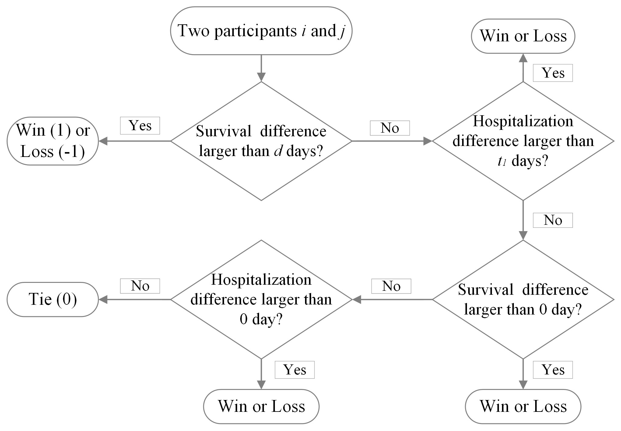
Figure 1: Procedure of the pairwise comparison between two participants, $i$ and $j$, in a SCWR with thresholds $(d,0)$ for the survival-time endpoint and $(t_{1},0)$ for the time-to-hospitalization endpoint.

In the 4-stage SCWR illustrated above, there are two opportunities for the time to hospitalization endpoint to contribute to the result of a pairwise comparison, as opposed to the single opportunity provided by WR. Such additional opportunity releases the strict hierarchy. As two extreme examples, when $d=+\infty,t_{1}=0$, SCWR prioritizes the time to hospitalization endpoint strictly like WR prioritizes the survival time endpoint. In contrast, when $d=0,t_{1}=0$, SCWR reduces to WR. Therefore, by varying the thresholds, one may control the priority between two endpoints from one end to the other. Such flexibility allows the convenient inclusion of clinical priors.

2.3 Adaptive thresholds

In this section, we introduce a pre-specified data-driven adaptive approach to choose the thresholds in the absence of sufficient clinical information. This adaptive approach is based on the quantile of survival-time and time-to-hospitalization differences among all pairwise comparisons. The proposed adaptive approach helps select the thresholds in a more intuitive way and has the adapting property of bypassing the random differences while detecting the true treatment effects on the survival-time endpoint (i.e., the higher layer).

To begin with, we define two sequences of all non-zero differences in pairwise comparisons among non-censored participants for survival time and time to hospitalization accordingly:

$$\mathbb{D} = \left\{|D_{i}-D_{j}|:\forall i,j\in\{1,2,...,n\},(D_{i}-D_{j})\Delta_{Di}\Delta_{Dj}\neq 0|\right\},$$

$$\mathbb{T}_{1} = \left\{|T_{1i}-T_{1j}|:\forall i,j\in\{1,2,...,n\},(T_{1i}-T_{1j})\Delta_{1i}\Delta_{1j}\neq 0|\right\}.$$

Such two sequences take comparisons between two participants from the same (i.e., both receive treatment or control) or contrasting groups (i.e., one receives treatment and the other receives control) into account, which is essential for gaining the adapting property (will be discussed shortly). Then, with the calipers $c_{1},c_{2}\in[0,1]$ specified, calculate the empirical $c_{1},c_{2}$ quantile values of these two sequences correspondingly, denoted as $q_{D}^{c_{1}}=\hat{q}_{c_{1}}(\mathbb{D})$ and $q_{1}^{c_{2}}=\hat{q}_{c_{2}}(\mathbb{T}_{1})$. Ultimately, set $(d,t_{1})=(q_{D}^{c_{1}},q_{1}^{c_{2}})$, where, loosely speaking, the relationship between $c_{1}$ and $c_{2}$ controls the weights of survival and hospitalization information. Intuitively, a larger caliper $c$ corresponds to a larger threshold, which indicates paying less attention to an endpoint. Therefore, $c_{1}\leq c_{2}$ is usually adopted as we shall still prioritize the higher layer even though the strict hierarchy is intended to be released. The influence of calipers on the weight between endpoints is more predictable and intuitive than that of thresholds themselves since the effect of thresholds relies on their relative scale with the observed differences. This helps make more confident choices on the tuning parameters.

To control the weight more straightforwardly, we consider employing $c_{1}=c_{2}=c$ and a weight parameter $w>0$: after obtaining $q_{D}^{c}=\hat{q}_{c}(\mathbb{D})$ and $q_{1}^{c}=\hat{q}_{c}(\mathbb{T}_{1})$, we set $(d,t_{1})=(q_{D}^{c},q_{1}^{c}/w)$, where the value of $w$, instead of the relationship between $c_{1}$ and $c_{2}$ controls the weight between two endpoints. A smaller $w$ indicates paying less attention to the time to hospitalization endpoint, as it makes the threshold for this endpoint larger. Since the remaining tuning parameters are $w,c$, we denote the resulted $\mathrm{SCWR}(q_{D}^{c},q_{1}^{c}/w,0,0)$ as $\mathrm{WASCWR}(w)^{c}$, which stands for weighted adaptive SCWR with weight $w$ and shared caliper $c$.

In the above adaptive threshold system, note that in the construction of adaptive thresholds, only non-zero differences are included in the sequences to exclude the results of self-comparison and ties. This ensures the subsequent quantiles are non-trivial (i.e., $d\neq 0,t_{1}\neq 0$). The caliper $c$ then indicates $c$ smallest non-zero absolute differences are insufficient in Stage 1&2. Based on our experience, we recommend using $c=20\%$ as the default value when clinical priors are not enough to make an informative change, and its impact on WASCWR will be demonstrated in the simulation section. When the default caliper value is employed, for simplicity, we omit the superscript $c=20\%$ in the above notations and denote $q_{D}=q_{D}^{20\%}=\hat{q}_{20\%}(\mathbb{D}),q_{1}=q_{1}^{20\%}=\hat{q}_{20\%}(\mathbb{T}_{1}),\mathrm{WASCWR}(w)=\mathrm{WASCWR}(w)^{20\%}$. As for the weight parameter $w$, a smaller $w$ assigns a smaller weight to the time-to-hospitalization endpoint by elevating the thresholds for differences in the time to hospitalization to be sufficient in Stage 2. Since the differential clinical importance between two endpoints is already addressed by the hierarchy and the caliper, the default value $w=1$ is often an adequate choice without external informative clinical knowledge. In addition, we will show that WASCWR is generally robust to the choice of several common values of $w$ through simulation so that different choices of $w$ will not influence the test in a dramatic way.

In addition to confident-to-specify tuning parameters, the adaptive thresholds have the adapting property, i.e., tending to detect true treatment effects while removing random differences efficiently on the survival time layer. As a result of this property, if the treatment only has an effect on extending the time to hospitalization, WASCWR affords much higher power than WR. On the other hand, WASCWR maintains similar power with WR when the treatment only has an effect on survival time. This adapting property is brought by obtaining the thresholds with pooled participants (i.e., including comparison results of pairs from both contrasting and same treatment groups) and applying them to the comparison between treatment and control groups. If there is no treatment effect on the survival-time layer, the distribution of survival-time difference between a pair of participants from contrasting groups will be similar to a pair from pooled participants. In this case, taking the recommended default $c=20\%$ as an example, the 20% quantile threshold concludes around 20% of non-zero differences are insufficient in comparisons between treatment and control participants on the survival-time layer. For those insufficient pairs, time-to-hospitalization differences will be considered, which allows the random differences on the time-to-death layer to contribute less to the final win-loss scores. On the contrary, if there are treatment effects on the survival-time layer, the distribution of absolute survival differences between a pair of participants from contrasting groups will be shifted towards a higher value compared with a pair from pooled participants. In this case, the 20% quantile threshold concludes less than 20% of comparisons between contrasting participants on the survival-time layer to be insufficient due to the shifting. Moreover, the degree of shifting positively depends on the strength of the effect. Given the advantage of this adapting property, employing adaptive thresholds is recommended for SCWR unless there are strong clinic priors for specifying thresholds.

2.4 Generalization of the shrinking coarsened win ratio with multiple thresholds and multiple non-fatal events

In Section 2.2, we introduced the 4-stage SCWR with survival and time to hospitalization endpoints. With such two endpoints, we may consider having $L\geq 1$ non-zero thresholds for each of them, namely $\left\{d_{1},d_{2},...,d_{L}>0\right\}$ for survival time and $\left\{t_{11},t_{12},...,t_{1L}>0\right\}$ for the nonfatal event. Given these two series of thresholds, the win-loss score for the pair comparison between $i$ and $j$ in this $2(L+1)$-stage SCWR, SCWR$(d_{1},t_{11},d_{2},t_{12},...,d_{L},t_{1L},0,0)$ is:

$$U_{ij}(d_{1},t_{11},d_{2},t_{12},...,d_{L},t_{1L},0,0)$$

$$= \mathscr{D}_{ij}(d_{1})+\left(1-\mathscr{D}^{2}_{ij}(d_{1})\right)\mathscr{T}_{ij1}(t_{11})+\left(1-\mathscr{D}^{2}_{ij}(d_{1})\right)\left(1-\mathscr{T}^{2}_{ij1}(t_{11})\right)\mathscr{D}_{ij}(d_{2})$$

$$+ \left(1-\mathscr{D}^{2}_{ij}(d_{1})\right)\left(1-\mathscr{T}^{2}_{ij1}(t_{11})\right)\left(1-\mathscr{D}^{2}_{ij}(d_{2})\right)\mathscr{T}_{ij1}(t_{12})+...$$

$$+ \prod_{l=1}^{L}\left[\left(1-\mathscr{D}^{2}_{ij}(d_{l})\right)\left(1-\mathscr{T}^{2}_{ij1}(t_{1l})\right)\right]\mathscr{D}_{ij}(0)$$

$$+ \prod_{l=1}^{L}\left[\left(1-\mathscr{D}^{2}_{ij}(d_{l})\right)\left(1-\mathscr{T}^{2}_{ij1}(t_{1l})\right)\right]\left(1-\mathscr{D}^{2}_{ij}(0)\right)\mathscr{T}_{ij1}(0).$$

In addition, it is possible to encounter more than one nonfatal events in a study. For the $K\geq 1$ nonfatal events, we define $T_{ki},(k=1,2,...,K)$ as the observed time to the nonfatal events (e.g., hospitalization, stroke, ischemia) of $i$, and $\Delta_{ki}$ as the corresponding censoring indicator for the $k$th nonfatal event. With one non-zero threshold $t_{k1}$ for each nonfatal event, the comparison functions for nonfatal events are then:

$$\mathscr{T}_{ijk}(t_{k1}) = I\left(|T_{ki}-T_{kj}|\geq t_{k1}\right)$$

$$\times\left[(1-\Delta_{ki})(1-\Delta_{kj})\text{Sign}(T_{ki}-T_{kj})+\Delta_{ki}(1-\Delta_{kj})I(T_{ki}>T_{kj})+(1-\Delta_{ki})\Delta_{kj}I(T_{ki}<T_{kj})\right],$$

$$~{}~{}~{}k=1,\ldots,K.$$

The SCWR formed by the survival time (with one non-zero threshold $d$) and $K$ nonfatal events can be decomposed into the following $2(K+1)$ components:

$$U_{ij1}=\mathscr{D}_{ij}(d),$$

$$U_{ij2}=\left(1-\mathscr{D}^{2}_{ij}(d)\right)\mathscr{T}_{ij1}(t_{11}),$$

$$U_{ij3}=\left(1-\mathscr{D}^{2}_{ij}(d)\right)\left(1-\mathscr{T}^{2}_{ij1}(t_{11})\right)\mathscr{T}_{ij2}(t_{21}),$$

$$...,$$

$$U_{ij,K+1}=\left(1-\mathscr{D}^{2}_{ij}(d)\right)\prod_{k=1}^{K-1}\left(1-\mathscr{T}^{2}_{ijk}(t_{k1})\right)\mathscr{T}_{ijK}(t_{K1}),$$

$$...,$$

$$U_{ij,2(K+1)}=\left(1-\mathscr{D}^{2}_{ij}(d)\right)\prod_{k=1}^{K}\left(1-\mathscr{T}^{2}_{ijk}(t_{k1})\right)\left(1-\mathscr{D}^{2}_{ij}(0)\right)\prod_{k=1}^{K-1}\left(1-\mathscr{T}^{2}_{ijk}(0)\right)\mathscr{T}_{ijK}(0).$$

By summing the above components, the final win-loss score for the pair comparison between $i$ and $j$ is:

$$U_{ij}(d,t_{11},t_{21},...,t_{K1},0,...,0)=\sum_{s=1}^{2(K+1)}U_{ijs}.$$

Based on the above two scenarios, in the most general scenario, for survival time and $K\geq 1$ nonfatal events, we may specify $L\geq 1$ non-zero thresholds for each of them to form the $(K+1)(L+1)-$stage SCWR. Denote non-zero thresholds for survival time as $\left\{d_{1},d_{2},...,d_{L}>0\right\}$, and for the $k$th nonfatal event as $\left\{t_{k1},t_{k2},...,t_{kL}>0\right\}$. The general expression for the win-loss score of pair comparison between $i$ and $j$ becomes:

$$U_{ij}(d_{1},t_{11},t_{21},...,t_{K1},d_{2},t_{12},t_{22},...,t_{K2},...,d_{L},t_{1L},t_{2L},...,t_{KL},0,...,0)$$

$$= \mathscr{D}_{ij}(d)+\left(1-\mathscr{D}^{2}_{ij}(d_{1})\right)\mathscr{T}_{ij1}(t_{11})+...+\left(1-\mathscr{D}^{2}_{ij}(d_{1})\right)\prod_{k=1}^{K-1}\left(1-\mathscr{T}^{2}_{ijk}(t_{k1})\right)\mathscr{T}_{ijK}(t_{K1})+...$$

$$+ \left(1-\mathscr{D}^{2}_{ij}(d_{1})\right)\left(1-\mathscr{D}^{2}_{ij}(d_{2})\right)\prod_{k=1}^{K}\left(1-\mathscr{T}^{2}_{ijk}(t_{k1})\right)\prod_{k=1}^{K-1}\left(1-\mathscr{T}^{2}_{ijk}(t_{k2})\right)\mathscr{T}_{ijk}(t_{K2})+...$$

$$+ \prod_{l=1}^{L}\left(1-\mathscr{D}^{2}_{ij}(d_{l})\right)\prod_{l=1}^{L}\prod_{k=1}^{K}\left(1-\mathscr{T}^{2}_{ijk}(t_{kl})\right)\left(1-\mathscr{D}^{2}_{ij}(0)\right)\prod_{k=1}^{K-1}\left(1-\mathscr{T}^{2}_{ijk}(0)\right)\mathscr{T}_{ijK}(0).$$

The adaptive thresholds proposed in Section 2.3 are also applicable in more general settings. For the survival time and $K$ nonfatal events, we define $K+1$ sequences of all non-zero difference in pair comparisons as:

$$\mathbb{D} = \left\{|D_{i}-D_{j}|:\forall i,j\in\{1,2,...,n\},(D_{i}-D_{j})\Delta_{Di}\Delta_{Dj}\neq 0|\right\},$$

$$\mathbb{T}_{k} = \left\{|T_{ki}-T_{kj}|:\forall i,j\in\{1,2,...,n\},(T_{ki}-T_{kj})\Delta_{ki}\Delta_{kj}\neq 0|\right\},~{}~{}~{}k=1,\ldots,K.$$

The empirical $c$ quantile values of these sequences are then $q_{D}^{c},q_{1}^{c},q_{2}^{c},...,q_{K}^{c}$. With $K$ weights for the nonfatal events $\{w_{1},w_{2},..,w_{K}\}$, we have WASCWR$(w_{1},w_{2},..,w_{K})^{c}$ as SCWR$(d=q_{D}^{c},t_{11}=q_{1}^{c}/w_{1},t_{21}=q_{2}^{c}/w_{2},...,t_{K1}=q_{K}^{c}/w_{K})$.

3 Simulation Study

In this section, we examine the performance of SCWR empirically via simulation. We first compare SCWR with WR regarding empirical power, validate its ability to control type I error, and then analyze the influence that caliper $c$ and weight $w$ have on the empirical power achieved by SCWR. Although the proposed SCWR method can accommodate multiple nonfatal events, without loss of generality, we focus on the simpler setting with survival-time and time-to hospitalization-endpoints for illustration.

3.1 Simulation setup

We consider a two-arm clinical trial with a total sample size $n=2000$ and equal allocation, where half of them are assigned to the treatment group $Z=1$ and the other half to the control group $Z=0$. Using Copula, a popular approach for generating correlated random variables, we then simulate the two correlated times to represent true survival time in days and true days before hospitalization. Following Luo et al. [8], we adopt the Gumbel-Hougaard copula with a bivariate distribution that has exponential margins. Specifically, we let $h_{D}(Z)=\lambda_{D}\exp(-\alpha_{D}Z)$ be the hazard rate for death event, and $h_{T_{1}}(Z)=\lambda_{T_{1}}\exp(-\alpha_{T_{1}}Z)$ be the hazard rate for hospitalization event. Then, the vector of survival time and time to hospitalization (in days) $(D^{*},T_{1}^{*})$ has the joint survival function [8]:

$$P(D^{*}>y_{1},T_{1}^{*}>y_{2}|Z)=\exp\left\{-[(h_{D}(Z)y_{2})^{\beta}+(h_{T_{1}}(Z)y_{1})^{\beta}]^{(1/\beta)}\right\},$$

where $\beta\geq 1$ is the parameter that controls the correlation between two information (i.e., Kendall’s concordance: $1-1/\beta$). We fix parameters $\lambda_{T_{1}}=0.0022,\lambda_{D}=0.0008$ and let $\alpha_{D},\alpha_{T_{1}}\in\{0,0.1,0.2,0.3\}$, in which $\{0,0.1,0.2,0.3\}$ stand for no, very weak, weak, and modest treatment effects. Without loss of generality, we assume treatment is not worse than control (in terms of extending survival time or time to hospitalization). In our simulation, it is possible to have sample $i$ with $T_{1i}^{*}\geq D^{*}_{i}$, which indicates there is no hospitalization event for $i$. Observed survival time and time to hospitalization are then obtained by performing administrative censoring after $FU$ days of follow-up for all participants. A significance level of $\alpha=0.05$ for a two-sided test is employed throughout this simulation.

We compare WASCWR (with default weight and caliper choices, i.e., $\mathrm{WASCWR}(w=1)^{c=20\%}$) with WR and examine the performance of WASCWR under different choices of weights and calipers. Three key influential factors, follow-up time, treatment effect, and correlation between survival days and days before hospitalization, are varied and detailed in Table 1 for simulation scenarios S1-S8. Additional simulation results under more scenarios are presented in Supporting Information S1. The empirical power calculation is based on 2000 simulation replicates, and the empirical type I error rate calculation is based on 5000 replicates. All calculations are implemented in R. Main R packages used include gumbel [25], foreach [26], doParallel [27], dplyr [28], ggplot2 [29]. The reproducible R codes are available at GitHub (URL will be provided).

Table 1: Settings of treatment effect levels and correlations between survival-time and time-to-hospitalization endpoints in eight simulation scenarios

Scenario	Treatment Effect		Kendall’s Concordance
	Survival Time	Time to Hospitalization
S0	None	None	0
S1	None	Modest	0.5
S2	None	Modest	0
S3	Modest	None	0.5
S4	Modest	None	0
S5	Very weak	Weak	0.5
S6	Very weak	Weak	0
S7	Weak	Very Weak	0.5
S8	Weak	Very Weak	0

3.2 Performance of WASCWR

The empirical power of WR and WASCWR under simulation scenarios S1-S8 (i.e., under alternative hypothesis) is summarized in Figure 2. To begin with, in simulation scenarios S1&S2, WASCWR continuously increases the power gained by WR by allowing the information on the time-to-hospitalization layer to contribute to the inference about the treatment effect. The difference between WASCWR and WR is more apparent with longer follow-up time. Since longer follow-up time indicates more observed death events on the survival-time layer, which brings more random differences, WASCWR increases the power by allowing the time-to-hospitalization layer to be considered more and bypassing the random difference on the survival-time layer. With a shorter follow-up time, WR maintains good performance as lower death rates allow a larger contribution from the time-to-hospitalization layer to pairwise comparison results. In simulation scenarios S3&S4, the treatment effect is on the survival-time layer with random differences on the time-to-hospitalization layer. Although addressing the time-to-hospitalization layer more is expected to be harmful to power, WASCWR gains comparable power relative to WR in simulation scenario S4, which is a result of employing the proposed adaptive thresholds. In simulation scenario S3, however, it is noticeable that the added correlation between endpoints lowers the power of both methods while WASCWR suffers slightly more. This interesting phenomenon will be further analyzed and explained in Section 3.3.

In simulation scenarios S1-S4, we consider scenarios where there are only random differences on one of the endpoints to demonstrate the performance of WASCWR under extreme situations. In practice, however, if prior information indicates no treatment effect on an endpoint, including it in the hierarchical structure should be avoided for both WASCWR and WR. In simulation scenarios S5-S8, on the contrary, we consider more common situations where there are treatment effects on both endpoints but with different strengths. In simulation scenarios S5&S6, where the treatment effect on the survival-time endpoint is lower than that on the time-to-hospitalization endpoint, WASCWR increases the power. Similar to that in simulation scenarios S1&S2, a longer follow-up time may lower the power as more pairwise comparison results are determined by the survival-time endpoint, where only very weak treatment effect exists. WASCWR appears to be more robust in dealing with such a negative effect. Different from the trend in simulation scenarios S1&S2, the power trend here first increases from 250-day follow-up to 500-day follow-up and then starts to decrease, which is likely a result of the difference between having very weak and completely no treatment effects on the survival-time layer. Additionally, in simulation scenarios S7&S8, there is only very weak treatment effect on the time-to-hospitalization endpoint. Similarly to that in simulation scenario S4, WASCWR achieves comparable power with WR. Ultimately, the empirical type I error in simulation scenario S0 is presented in Table 2. Under the popular significance level $\alpha=0.05$, both WR and WASCWR control the type I error rates in a reasonable range around this nominal $\alpha$.

In summary, the proposed WASCWR has potentially better performance than the standard WR in terms of gaining power under multiple situations. This is mainly because of the correction of some results in pairwise comparisons. In a Wilcoxon-type test, including WR and WASCWR, the two most obvious ways to increase power are breaking the ties and increasing the sample size. However, when the information is not fully collected due to the follow-up time censoring, both of these two ways require the added information to contribute to the statistic in the right direction. For example, if the true treatment effect is positive, then the broken ties and the added samples need to show a positive treatment effect in general to increase the power. Therefore, WASCWR helps increase power even if there are no more ties broken or new samples added.

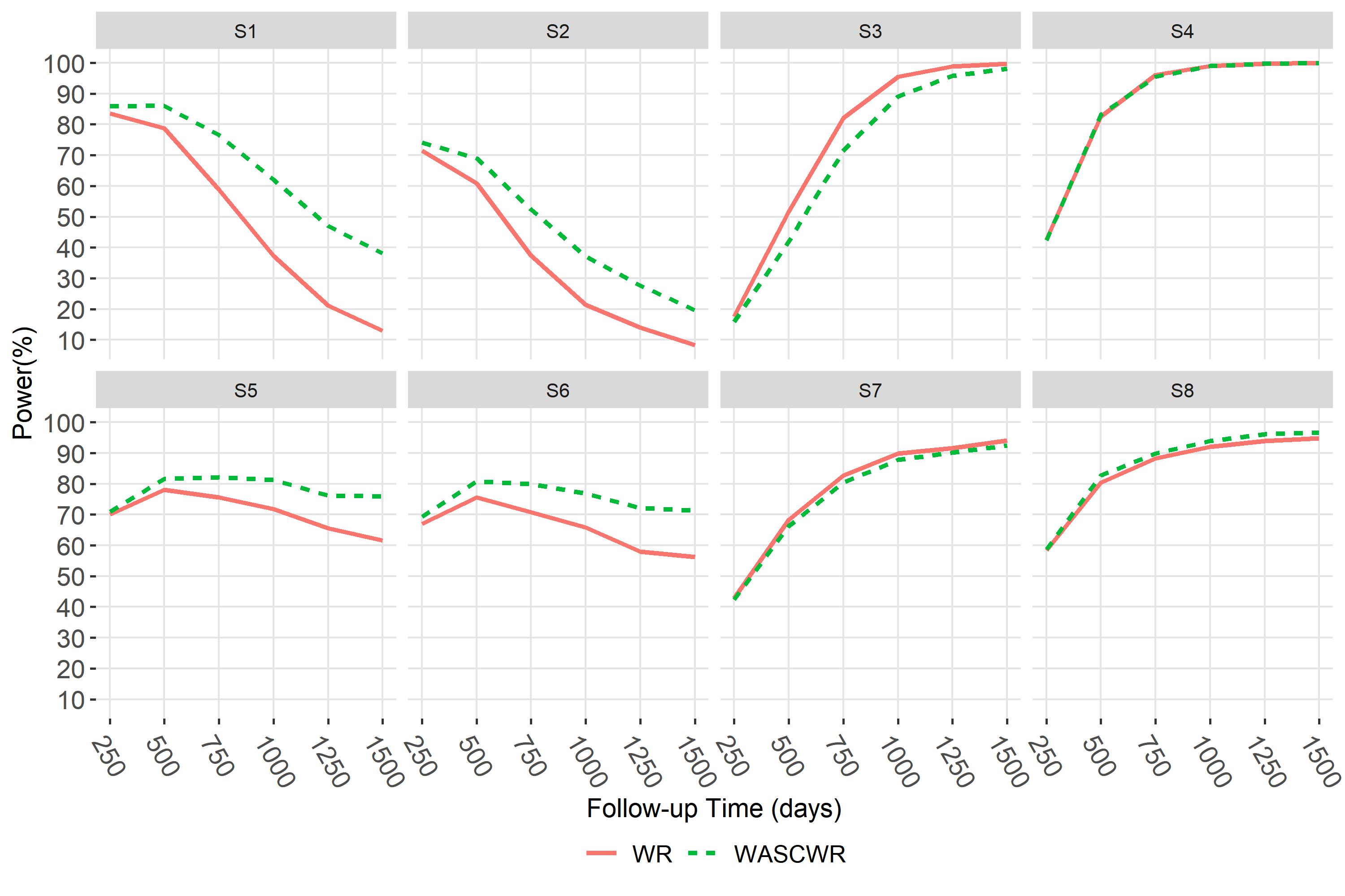
Figure 2: Empirical power of WASCWR and WR tests in simulation scenario: (S1) modest treatment effect on the time-to-hospitalization endpoint only, assuming a correlation between survival-time and time-to-hospitalization endpoints, (S2) modest treatment effect on the time-to-hospitalization endpoint only, assuming no correlation, (S3) modest treatment effect on the survival-time endpoint only, assuming a correlation, (S4) modest treatment effect on the survival-time endpoint only, assuming no correlation, (S5) very weak treatment effect on the survival-time endpoint and weak treatment effect on the time-to-hospitalization endpoint, assuming a correlation, (S6) very weak treatment effect on the survival-time endpoint and weak treatment effect on the time-to-hospitalization endpoint, assuming no correlation, (S7) weak treatment effect on the survival-time endpoint and very weak treatment effect on the time-to-hospitalization endpoint, assuming correlation, (S8) weak treatment effect on the survival-time endpoint and very weak treatment effect on the time-to-hospitalization endpoint, assuming no correlation

Table 2: Empirical type I errors (%) obtained by WASCWR and WR in under the null (simulation scenario S0).

Scenario	FU	WR	WASCWR
S0	500	4.96	4.64
S0	1000	4.58	4.54
S0	1500	5.26	5.32

3.3 Influence of the correlation

In this subsection, we present additional insights into the observed difference in power between simulation scenarios S3&S4. The win ratios (full spelling for the ratio measures themselves, and WR for the method) in simulation scenarios S3&S4 with 750-day follow-up time are decomposed to stage-level and averaged across 2000 replicates in Table 3. Results from other follow-up time are included in Supporting Information S2. The decomposition procedure presents the wins, losses, and ties obtained by the treatment group participants in each stage, where the ratio of the number of such wins to the number of such losses corresponds to the stage-level win ratio. For example, for WR under simulation scenario S3 in Table 3, the averaged wins (/losses) obtained in the survival-time layer is 37.21%(/27.60%). The 35.19% pairs with ties on the survival-time layer then get their time-to-hospitalization endpoint compared, resulting in 14.96% wins and 17.08% losses. The remaining 3.14% pairwise comparisons receive ties as their conclusions. In such a decomposition matrix, the percentages are all calculated based on the total number of pairwise comparisons between two contrasting participants. Therefore, the overall win ratio can be obtained by dividing the sum of stage-level wins by the sum of stage-level losses. In Table 3, the bolded values in the stage-level win ratio column are those obtained by the time-to-hospitalization layer. In simulation scenario S3, such values are less than one, as opposed to very close to one in simulation scenario S4. Although without any testing, the difference between around 0.80 and 1.00 in terms of the stage-level win ratios averaged across 2000 replicates is non-negligible. In simulation scenario S3, the marginal correlation between the survival-time and time-to-hospitalization endpoints influences the appearance of the time-to-hospitalization endpoint conditioning on receiving ties in the survival-time layer. As a result, although there is no treatment effect on the time-to-hospitalization endpoint marginally, the spurious negative “treatment effects” are observed on the pairwise comparisons between participants with no difference on the survival-time layer. Such spurious negative “treatment effects” are the core reason for the lowered power in detecting the true positive treatment effects. These results emphasize the need for careful consideration when including additional endpoints in the hierarchical structure in practice. A layer that appears non-harmful in terms of power may behave differently after conditioning on the results of higher layers.

Table 3: Stage-level decomposition of win ratios in simulation scenarios S3&S4 with 750-day follow-up time averaged across 2000 replicates. In WR, stages 1&2 represent survival-time and time-to-hospitalization endpoints correspondingly. In WASCWR, stages 1&3 represent the survival-time endpoint, and stages 2&4 represent the time-to-hospitalization endpoints. The stage-level win ratios with the bolded values correspond to those relevant to the time-to-hospitalization endpoint.

Scenario	Method	Stage	Win (%)	Tie (%)	Loss (%)	Stage-level win ratio
3	WR	1	37.21	35.19	27.60	1.35
		2	14.96	3.14	17.08	0.88
	SCWR	1	30.70	48.00	21.30	1.44
		2	15.20	14.33	18.47	0.82
		3	3.40	7.96	2.97	1.14
		4	2.38	3.14	2.45	0.97
4	WR	1	37.19	35.19	27.62	1.35
		2	16.91	1.33	16.94	1.00
	SCWR	1	30.68	48.00	21.32	1.44
		2	17.35	13.27	17.37	1.00
		3	3.38	6.60	3.29	1.03
		4	2.63	1.33	2.64	1.00

3.4 Influence of the caliper

In this subsection, we demonstrate the influence of caliper choices on adaptive thresholds. In addition to the default caliper ($c=20\%$), we consider $c=10\%,40\%$, and the combined calipers. The combined caliper is an eight-stage SCWR that progressively employs $c=40\%,20\%,10\%$ calipers: $\mathrm{SCWR}\left(q_{D}^{40\%},q_{1}^{40\%},q_{D}^{20\%},q_{1}^{20\%},q_{D}^{10\%},q_{1}^{10\%},0,0\right).$ The results are presented in Table 4. In this simulation, a larger caliper tends to better bypass the random differences and a smaller caliper tends to better detect the treatment effect on the survival-time layer. The combined caliper is slightly enhanced by its more stages in bypassing random differences. Increasing the caliper from 10% to 20% and 40%, the incremental in simulation scenarios S1, S2, S5, and S6, where the primary treatment effects are on the time-to-hospitalization layer, is generally larger than the loss in the rest simulation scenarios, where the effects are primarily on the survival-time layer. This is as expected since the mechanism of adaptive thresholds tends to keep detecting truly existing treatment effects while bypassing random differences. The combined caliper approach achieves the highest power under simulation scenarios S1, S2, S5, and S6, which is likely a result of its enhanced structure that favors bypassing the random differences. In general, WASCWR is robust to the choice of caliper values as no rapid change in the performance of WASCWR with different calipers is observed under most simulation scenarios.

Table 4: Empirical power (%) obtained by WASCWR with different calipers $c$ in simulation scenarios S1-S8

Scenario	FU	Caliper-10%	Caliper-20%	Caliper-40%	Combined Caliper
S1	500	85.65	87.10	82.90	90.05
S1	1000	54.15	62.70	61.50	75.45
S1	1500	27.55	39.95	44.35	59.35
S2	500	65.95	69.40	70.90	75.45
S2	1000	29.95	37.35	47.50	52.75
S2	1500	13.00	19.80	30.55	36.25
S3	500	42.90	41.55	44.85	36.95
S3	1000	91.50	88.85	89.00	81.80
S3	1500	99.30	98.60	98.20	95.50
S4	500	84.30	83.90	83.30	83.25
S4	1000	99.20	99.10	99.00	98.95
S4	1500	99.80	99.85	99.80	99.85
S5	500	80.55	81.55	79.70	82.95
S5	1000	76.95	80.00	79.70	83.45
S5	1500	67.90	72.45	74.60	79.70
S6	500	77.50	79.50	79.30	81.80
S6	1000	73.15	77.10	81.35	83.75
S6	1500	65.30	72.10	79.55	82.00
S7	500	68.20	67.85	69.10	66.40
S7	1000	88.05	87.35	87.70	85.55
S7	1500	94.40	93.85	93.35	91.85
S8	500	82.10	82.75	82.60	83.35
S8	1000	93.00	93.55	94.30	94.50
S8	1500	96.15	96.90	97.25	97.60

3.5 Influence of the weight

In this subsection, we show the influence of weight choices on adaptive thresholds. Alternative to the default weight choice $w=1$, we include $w=0.1,0.3,0.5$. In the resulting four candidate methods, WASCWR(1), WASCWR(0.5), WASCWR(0.3), WASCWR(0.1), a smaller $w$ addresses the survival-time endpoint more. According to the results presented in Table 5, in simulation scenarios S1, S2, S5, and S6, where the treatment effects are primarily on the time-to-hospitalization layer, smaller $w$ leads to lower power. This is as expected since addressing the higher-layer endpoint naturally brings more difficulty in detecting the treatment effect on the lower layer. In simulation scenarios S3, S4, S7, and S8, where the treatment effects are primarily on the survival-time layer, comparable power is usually achieved by different choices of $w$. These indicate WASCWR is robust to the choice of $w$ in terms of maintaining the capacity to detect treatment effects on the survival-time layer. Such appealing properties are again ensured by the mechanism of the adaptive threshold system.

Table 5: Empirical power (%) obtained by WASCWR with different weights $w$ in simulation scenarios S1-S8

Scenario	FU	WASCWR(0.1)	WASCWR(0.3)	WASCWR(0.5)	WASCWR(1.0)
S1	500	79.00	79.45	82.15	85.90
S1	1000	38.65	46.30	55.15	64.00
S1	1500	12.40	21.70	28.95	37.50
S2	500	60.00	62.45	66.25	68.30
S2	1000	21.35	28.45	32.30	36.05
S2	1500	9.50	14.85	18.20	20.80
S3	500	51.90	50.75	47.50	41.60
S3	1000	95.10	93.85	91.95	88.15
S3	1500	99.50	98.95	98.55	97.70
S4	500	82.10	82.10	82.10	82.05
S4	1000	99.15	99.10	99.05	99.10
S4	1500	99.95	99.95	99.95	99.95
S5	500	78.25	78.55	79.80	81.50
S5	1000	70.55	73.70	76.35	79.10
S5	1500	61.00	66.40	70.10	73.05
S6	500	74.70	75.90	77.10	78.50
S6	1000	64.35	71.00	73.90	75.75
S6	1500	59.85	68.05	71.25	73.60
S7	500	71.40	71.00	70.80	70.00
S7	1000	88.20	87.55	86.55	85.45
S7	1500	94.60	93.95	93.40	92.50
S8	500	82.05	82.60	83.60	84.10
S8	1000	93.00	93.85	94.45	94.75
S8	1500	96.15	96.95	97.45	97.70

4 Case Study

In this section, we apply SCWR to analyze the Digitalis Investigation Group (DIG) trial (ClinicalTrials.gov identifier: NCT00000476). This clinical trial investigated the effect of digoxin on patients with heart failure. Patients who had heart failure and a left ventricular ejection fraction of 0.45 or less were eligible for the primary randomization. This study was neutral for its primary outcome of all-cause mortality but evaluated both death and hospitalization events. When these two outcomes were analyzed separately, treatment effects appeared mainly on the hospitalization outcomes. Alternatively, we hereby employ SCWR and WR to reanalyze this dataset. In this case study, both death and hospitalization outcomes are analyzed in the time-to-event form with the right censoring information taken into account (i.e., survival time and time to hospitalization). In developing the hierarchy structure, time to (all-cause) death is included as the higher layer, and time to (all-cause) hospitalization is included as the lower layer in both SCWR and WR. To bring new insight into this dataset, we focus on key subgroups from the trial population and add stratification for better adjustment in this analysis. To be specific, we focus on the subgroup population with New York Heart Association (NYHA) functional class III or IV and stratify by ejection fraction ($<0.25$ or $0.25-0.45$), cause of heart failure (ischemic or nonischemic), and age ($<70$ or $\geq 70$). The number of patients within each stratum is presented in Table 6. For SCWR, the adaptive thresholds with default weight and caliper ($w=1,c=20\%$) are adopted. The results are shown in Table 7.

Table 6: Number of patients within each stratum

	Ejection fraction < 0.25
	Ischemic		Nonischemic
	Age < 70	Age >= 70	Age < 70	Age >= 70
Treatment	231	82	102	53
Control	190	119	136	39
	Ejection fraction 0.25 0.45
	Ischemic		Nonischemic
	Age < 70	Age >= 70	Age < 70	Age >= 70
Treatment	286	188	113	61
Control	277	184	100	56

Table 7: Hypothesis testing results of SCWR and WR

	Win ratio	P-value
SCWR	1.293	0.0326
Standard WR	1.262	0.0553

Both methods result in similar estimates of the win ratio, 1.293 with SCWR and 1.262 with WR. However, SCWR yields a smaller P-value (i.e., lower variance of the estimated win ratio) and concludes significant treatment effects (under the 0.05 significance level). It is noticeable that here in this study, the treatment effects are weak on the survival-time endpoint and relatively stronger on the time-to-hospitalization endpoint, where the strict priority given to the survival-time layer lowers the power of WR. This shows that SCWR can advance from WR by a higher capacity in detecting the treatment effect under certain situations. In this case study, we report P-values for the hypothesis tests evaluating the absence or presence of a treatment effect and interpret statistical significance at the 0.05 level for the purposes of demonstration. Nevertheless, we recognize that interpreting study results should not depend solely on whether a P-value is greater than or less than a single cutoff point like 0.05.

5 Discussion

In this study, we develop a hypothesis-testing method for composite endpoints with a hierarchical structure. Based on the popular WR, the proposed SCWR adds layers with shrinking coarsened thresholds to pairwise comparisons. SCWR gains higher power than the standard WR by correcting the results of pairwise comparisons to bypass random differences on the higher layer. Weighted adaptive thresholds are also developed to reduce the difficulty of determining the coarsened thresholds solely with clinical priors. With the synthetic datasets, we compare the performance of WASCWR and WR while addressing the influence of scheduled follow-up lengths, strengths of treatment effects, and correlation levels between the two endpoints. The numerical results show that WASCWR outperforms WR when the effect is mainly on the lower layer and maintains comparable power when the effect is mainly on the higher layer. The stratified versions of both WASCWR and WR are then applied to analyze the DIG trial data. Their performance on the DIG trial data aligns with the observations in the numerical comparison and indicates the advantages that SCWR has over WR under certain circumstances.

In WASCWR, there are two tuning parameters that need to be specified: weight $w$ and caliper $c$. Based on our experience and the robustness of WASCWR under different choices of such two tuning parameters, we recommend using $w=1,c=20\%$ as the default when clinical priors are not available. However, their values may be selected in an informed way. Therefore, we investigate several different choices of $c$ in the simulations to provide additional insights into their working mechanisms. In addition to different choices of $c$, the combined caliper approach we included in the simulation study might be an alternative (e.g., $\mathrm{SCWR}\left(q_{D}^{40\%},q_{1}^{40\%},q_{D}^{20\%},q_{1}^{20\%},q_{D}^{10\%},q_{1}^{10\%},0,0\right)$ as employed in Section 3.4). The performance of the combined caliper approach tends to rely mainly on the largest caliper it contains as the priority is given to such caliper by the hierarchy. It is worth noting that extra attentions are given to the lower layer (i.e., time-to-hospitalization in our example) in this approach since more opportunities for the lower layer to contribute pairwise comparison results are provided by each one of the added calipers. In this combined caliper approach, the additional computation time brought by the added stages may also need to be considered, particularly when the study sample size is large or repeated calculations are required (e.g., bootstrap or permutation method in estimating the variance and constructing the confidence interval). When $c$ is fixed, the weight $w\in[0,1]$ increases the adaptive threshold of the lower layer to address the higher-layer endpoint. Since the reciprocal function in the $q_{1}^{c}/w$ structure is not on a linear scale, care is needed to use a relatively small $w$. Apart from adopting the reciprocal function, one may consider the two-caliper structure ($c_{1},c_{2}$). This architecture employs a larger quantile to increase the lower-layer threshold. When a small $w$ is desired, one may employ this approach and adjust $c_{2}$ to avoid the potential trivial stage caused by $w$ close to zero. Despite the flexibility of the proposed adaptive threshold system, the structure ($w,c$) or ($c_{1},c_{2}$) should be pre-specified, or with appropriate methods to control for the nominal type I error rate if post hoc changes are performed.

There are a few limitations and potential extensions that we may address in future studies. First, similar to WR, the estimated win ratios in SCWR could be affected by censoring of time-to-event endpoints [12]. The existing methods to address right censoring such as inverse-probability-of-censoring weighting [13, 14] may be adapted to SCWR, and are worth investigation in future research. Second, the proposed shrinking coarsened method can be extended beyond the win ratio measure. Although the proposed SCWR is developed to estimate and test the win ratio, the key idea, i.e., establishing comparison functions (e.g., $\mathscr{D}_{ij}(d),\mathscr{T}_{ij1}(t_{1})$) by applying thresholds successively and alternating across endpoints to release the strict hierarchy, can be naturally adapted to other win functions and statistics. For example, to address ties in pairwise comparisons, one may apply the comparison functions with adaptive thresholds developed for SCWR to calculate the shrinking coarsened win odds [17], and conduct inference accordingly. Third, in addition to the time-to-event endpoints, it is possible to include other types of outcome measures in SCWR. For example, to include a continuous outcome, one only need to omit the censoring indicator, i.e., regarding all records as not censored. Finally, by employing the comparison functions defined in SCWR, the shrinking coarsened method can be extended to the existing regression frameworks developed for win functions [20, 21, 22]. Such extensions may help leverage covariate effects in estimation and inference. Future research may further explore potential extensions for even wider applications.

Supporting Information

Appendix S1 Additional simulation scenarios

In this section, we include simulation results for 8 additional simulation scenarios S9-S16, as listed in Table S-1. The simulation setup is the same as that in the main text for simulation scenarios S1-S8. The table version of the power achieved by WASCWR and WR in simulation scenarios S1-S8 is also included.

Table S-1: Settings of treatment effect levels and correlations between survival-time and time-to-hospitalization endpoints in eight additional simulation scenarios

Scenario	Treatment Effect		Kendall’s Concordance
	Survival Time	Time to Hospitalization
S9	Weak	None	0.5
S10	Weak	None	0
S11	Weak	Weak	0.5
S12	Weak	Weak	0
S13	Weak	Modest	0.5
S14	Weak	Modest	0
S15	Very weak	Very weak	0.5
S16	Very weak	Very weak	0

S1.1 Performance of WASCWR

In simulation scenarios S9&S10, where the weak treatment effect is on the survival-time endpoint only, WASCWR and WR achieve comparable power when correlation is not assumed, and the difference in power is larger with correlation assumed. Such observation is similar to that in simulation scenarios S3&S4. In simulation scenarios S11-S14, WASCWR and WR perform well as the treatment effects are on both endpoints and the overall strength of such effects is strong enough. In simulation scenarios S15&S16, where very weak treatment effects are on both endpoints, WASCWR achieves slightly higher power than WR. This is likely a result of providing more chances for the time-to-hospitalization endpoint, where the treatment effect is easier to observe, as the administrative censoring rate is usually lower than that for the survival-time endpoint.

Table S-2: Empirical power (%) obtained by WASCWR and WR in simulation scenarios S1-S16

Scenario	FU	WR	WASCWR	Scenario	FU	WR	WASCWR
1	250	83.55	85.85	9	250	11.75	10.95
1	500	78.75	86.05	9	500	29.55	23.05
1	750	58.75	76.60	9	750	52.70	42.60
1	1000	37.30	61.95	9	1000	70.70	57.90
1	1250	21.05	47.05	9	1250	83.10	70.05
1	1500	12.95	38.20	9	1500	88.15	78.00
2	250	71.50	74.15	10	250	23.55	23.50
2	500	60.85	68.95	10	500	51.75	51.10
2	750	37.40	52.35	10	750	73.35	72.55
2	1000	21.35	37.15	10	1000	84.70	84.10
2	1250	13.95	27.60	10	1250	89.80	89.20
2	1500	8.25	19.60	10	1500	92.35	91.90
3	250	17.65	15.80	11	250	82.15	82.15
3	500	51.70	41.95	11	500	93.90	94.25
3	750	82.15	71.45	11	750	95.55	96.15
3	1000	95.55	89.15	11	1000	96.25	97.00
3	1250	98.80	95.85	11	1250	96.10	97.35
3	1500	99.75	98.15	11	1500	96.85	98.00
4	250	42.65	42.40	12	250	87.05	87.90
4	500	82.60	83.05	12	500	95.70	97.00
4	750	96.05	95.45	12	750	96.45	97.90
4	1000	98.95	99.05	12	1000	97.10	98.65
4	1250	99.70	99.75	12	1250	97.30	99.00
4	1500	99.95	99.85	12	1500	97.20	98.90
5	250	70.10	71.00	13	250	96.35	96.50
5	500	78.05	81.50	13	500	99.35	99.45
5	750	75.60	82.20	13	750	99.55	99.75
5	1000	71.80	81.20	13	1000	99.30	99.85
5	1250	65.60	76.20	13	1250	99.15	99.95
5	1500	61.55	75.95	13	1500	98.90	99.60
6	250	67.00	69.40	14	250	98.00	98.40
6	500	75.65	80.80	14	500	99.30	99.70
6	750	70.85	80.00	14	750	99.25	99.75
6	1000	65.80	76.90	14	1000	99.00	99.65
6	1250	57.95	72.10	14	1250	98.75	99.85
6	1500	56.30	71.40	14	1500	98.55	99.75
7	250	42.90	42.35	15	250	31.15	30.95
7	500	68.25	66.30	15	500	41.95	42.80
7	750	82.70	80.40	15	750	47.25	48.75
7	1000	89.80	87.85	15	1000	47.60	50.10
7	1250	91.65	90.10	15	1250	47.80	50.10
7	1500	94.15	92.55	15	1500	50.90	53.95
8	250	58.40	58.65	16	250	36.55	37.35
8	500	80.45	82.70	16	500	46.50	49.95
8	750	88.20	89.90	16	750	47.15	52.45
8	1000	92.00	94.00	16	1000	48.25	54.00
8	1250	93.95	96.05	16	1250	50.45	58.15
8	1500	94.85	96.70	16	1500	47.20	56.60

S1.2 Influence of caliper

In simulation scenarios S9-S16, the performance of WASCWR is generally comparable under different caliper choices, including the combined caliper strategy, and those differences observed are as expected. In simulation scenario S9, increased caliper values and adopting the combined caliper strategy achieve lower power for addressing the time-to-hospitalization endpoint with spurious negative “treatment effects”. In simulation scenarios S15&S16, on the contrary, higher power is achieved by them due to the easier-to-observe treatment effects on the time-to-hospitalization endpoint.

Table S-3: Empirical power (%) obtained by WASCWR with different calipers $c$ in simulation scenarios S9-S16

Scenario	FU	Caliper-10%	Caliper-20%	Caliper-40%	Combined Caliper
S9	500	25.40	24.45	26.40	21.75
S9	1000	62.75	58.40	58.65	51.00
S9	1500	83.55	78.80	77.45	69.50
S10	500	51.45	51.15	51.30	50.55
S10	1000	85.20	85.00	84.30	83.20
S10	1500	92.95	92.80	91.55	91.25
S11	500	93.60	93.90	93.50	94.05
S11	1000	97.30	97.45	97.55	97.45
S11	1500	97.80	97.95	98.45	98.55
S12	500	96.25	96.90	97.00	97.55
S12	1000	98.25	98.75	99.20	99.35
S12	1500	98.10	98.85	99.10	99.15
S13	500	99.25	99.35	99.15	99.45
S13	1000	99.55	99.75	99.70	99.75
S13	1500	99.55	99.70	99.75	99.90
S14	500	99.25	99.30	99.25	99.45
S14	1000	99.65	99.75	99.85	99.90
S14	1500	99.05	99.50	99.70	99.80
S15	500	42.55	43.00	42.50	42.95
S15	1000	48.55	49.30	50.60	50.60
S15	1500	50.60	52.05	52.85	53.60
S16	500	48.10	49.15	49.75	51.70
S16	1000	52.10	54.45	58.15	59.75
S16	1500	54.05	58.15	61.35	62.95

S1.3 Influence of weight

In simulation scenarios S9-S16, the performance of WASCWR is generally comparable under different weight choices, including the combined caliper strategy, and those differences observed are as expected. In simulation scenario S9, increased weights achieve lower power for addressing the time-to-hospitalization endpoint with spurious negative “treatment effects”. In simulation scenarios S15&S16, on the contrary, higher power is achieved by increasing the weight due to the easier-to-observe treatment effects on the time-to-hospitalization endpoint.

Table S-4: Empirical power (%) obtained by WASCWR with different weights $w$ in simulation scenarios S9-S16

Scenario	FU	WASCWR(0.1)	WASCWR(0.3)	WASCWR(0.5)	WASCWR(1.0)
S9	500	29.85	29.20	27.30	24.40
S9	1000	72.80	69.30	65.40	60.70
S9	1500	88.15	85.15	82.10	78.45
S10	500	51.00	50.60	50.70	51.00
S10	1000	84.90	84.50	84.35	84.25
S10	1500	93.10	92.85	92.70	92.50
S11	500	93.40	93.50	93.80	94.05
S11	1000	96.60	97.10	97.40	97.50
S11	1500	96.75	97.15	97.35	97.60
S12	500	95.85	96.00	96.50	96.80
S12	1000	96.90	97.75	97.85	98.15
S12	1500	97.75	98.75	99.00	99.15
S13	500	99.70	99.75	99.80	99.80
S13	1000	99.40	99.50	99.50	99.75
S13	1500	98.55	99.05	99.20	99.45
S14	500	99.30	99.45	99.55	99.65
S14	1000	98.90	99.45	99.65	99.65
S14	1500	98.85	99.35	99.60	99.75
S15	500	40.80	41.00	41.20	41.65
S15	1000	48.35	50.00	50.65	51.35
S15	1500	47.90	49.80	50.20	51.15
S16	500	44.35	45.55	46.95	47.60
S16	1000	47.85	51.40	53.05	54.20
S16	1500	51.40	55.55	56.30	57.80

Appendix S2 Influence of correlation

In this section, we provide additional analysis of the influence that the correlation between survival-time and time-to-hospitalization endpoints has on the power. The overall win ratios are decomposed to endpoint-level, i.e., win ratios for the survival-time and time-to-hospitalization endpoints. In WR, comparison results in stages 1&2 are attributed to survival-time and time-to-hospitalization endpoints correspondingly. In WASCWR, stages 1&3 are attributed to the survival-time endpoint, and stages 2&4 are attributed to the time-to-hospitalization endpoint. In simulation scenario S3, both WASCWR and WR have their time-to-hospitalization endpoint win ratios less than 1, as opposed to those win ratios close to 1 in simulation scenario S4. Such comparison indicates the existence of spurious negative “treatment effects” introduced by the marginal correlation between survival-time and time-to-hospitalization endpoints.

Table S-5: Endpoint-level decomposition of win ratios in simulation scenarios S3&S4 averaged across 2000 replicates.

Scenario	FU	WR			WASCWR
		Overall	Survival-time	Time-to-hospitalization	Overall	Survival-time	Time-to-hospitalization
S3	250	1.07	1.36	0.91	1.07	1.41	0.89
S3	500	1.12	1.35	0.89	1.11	1.41	0.87
S3	750	1.17	1.35	0.88	1.15	1.41	0.84
S3	1000	1.21	1.36	0.87	1.18	1.42	0.82
S3	1250	1.25	1.35	0.86	1.21	1.41	0.79
S3	1500	1.27	1.35	0.85	1.23	1.41	0.77
S4	250	1.12	1.36	1.00	1.12	1.38	1.00
S4	500	1.17	1.36	1.00	1.17	1.39	1.00
S4	750	1.22	1.35	1.00	1.21	1.39	1.00
S4	1000	1.25	1.35	1.00	1.25	1.39	1.00
S4	1250	1.28	1.35	1.00	1.28	1.40	1.00
S4	1500	1.30	1.35	1.00	1.30	1.40	1.00

References

- [1] Stuart J Pocock, Cono A Ariti, Timothy J Collier, and Duolao Wang. The win ratio: a new approach to the analysis of composite endpoints in clinical trials based on clinical priorities. European Heart Journal, 33(2):176–182, 2012.
- [2] Lu Mao and KyungMann Kim. Statistical models for composite endpoints of death and nonfatal events: a review. Statistics in Biopharmaceutical Research, 13(3):260–269, 2021.
- [3] Dianne M Finkelstein and David A Schoenfeld. Combining mortality and longitudinal measures in clinical trials. Statistics in Medicine, 18(11):1341–1354, 1999.
- [4] Samvel B Gasparyan, Folke Folkvaljon, Olof Bengtsson, Joan Buenconsejo, and Gary G Koch. Adjusted win ratio with stratification: calculation methods and interpretation. Statistical Methods in Medical Research, 30(2):580–611, 2021.
- [5] Nicholas A Fergusson, Tim Ramsay, Michaël Chassé, Shane W English, and Greg A Knoll. The win ratio approach did not alter study conclusions and may mitigate concerns regarding unequal composite end points in kidney transplant trials. Journal of Clinical Epidemiology, 98:9–15, 2018.
- [6] Kentaro Sakamaki and Takuya Kawahara. Statistical methods and graphical displays of quality of life with survival outcomes in oncology clinical trials for supporting the estimand framework. BMC Medical Research Methodology, 22(1):259, 2022.
- [7] Gaohong Dong, Junshan Qiu, Duolao Wang, and Marc Vandemeulebroecke. The stratified win ratio. Journal of Biopharmaceutical Statistics, 28(4):778–796, 2018.
- [8] Xiaodong Luo, Hong Tian, Surya Mohanty, and Wei Yann Tsai. An alternative approach to confidence interval estimation for the win ratio statistic. Biometrics, 71(1):139–145, 2015.
- [9] Ionut Bebu and John M Lachin. Large sample inference for a win ratio analysis of a composite outcome based on prioritized components. Biostatistics, 17(1):178–187, 2016.
- [10] Gaohong Dong, Di Li, Steffen Ballerstedt, and Marc Vandemeulebroecke. A generalized analytic solution to the win ratio to analyze a composite endpoint considering the clinical importance order among components. Pharmaceutical Statistics, 15(5):430–437, 2016.
- [11] Lu Mao. On the alternative hypotheses for the win ratio. Biometrics, 75(1):347–351, 2019.
- [12] D Oakes. On the win-ratio statistic in clinical trials with multiple types of event. Biometrika, 103(3):742–745, 2016.
- [13] Gaohong Dong, Lu Mao, Bo Huang, Margaret Gamalo-Siebers, Jiuzhou Wang, GuangLei Yu, and David C Hoaglin. The inverse-probability-of-censoring weighting (ipcw) adjusted win ratio statistic: an unbiased estimator in the presence of independent censoring. Journal of biopharmaceutical statistics, 30(5):882–899, 2020.
- [14] Gaohong Dong, Bo Huang, Duolao Wang, Johan Verbeeck, Jiuzhou Wang, and David C Hoaglin. Adjusting win statistics for dependent censoring. Pharmaceutical Statistics, 20(3):440–450, 2021.
- [15] Xiaodong Luo, Junshan Qiu, Steven Bai, and Hong Tian. Weighted win loss approach for analyzing prioritized outcomes. Statistics in Medicine, 36(15):2452–2465, 2017.
- [16] Marc Buyse. Generalized pairwise comparisons of prioritized outcomes in the two-sample problem. Statistics in Medicine, 29(30):3245–3257, 2010.
- [17] Edgar Brunner, Marc Vandemeulebroecke, and Tobias Mütze. Win odds: an adaptation of the win ratio to include ties. Statistics in Medicine, 40(14):3367–3384, 2021.
- [18] Song Yang and James Troendle. Event-specific win ratios and testing with terminal and non-terminal events. Clinical Trials, 18(2):180–187, 2021.
- [19] Song Yang, James Troendle, Daewoo Pak, and Eric Leifer. Event-specific win ratios for inference with terminal and non-terminal events. Statistics in Medicine, 41(7):1225–1241, 2022.
- [20] Lu Mao and Tuo Wang. A class of proportional win-fractions regression models for composite outcomes. Biometrics, 77(4):1265–1275, 2021.
- [21] Tuo Wang and Lu Mao. Stratified proportional win-fractions regression analysis. Statistics in Medicine, 41(26):5305–5318, 2022.
- [22] James Song, Johan Verbeeck, Bo Huang, David C Hoaglin, Margaret Gamalo-Siebers, Yodit Seifu, Duolao Wang, Freda Cooner, and Gaohong Dong. The win odds: statistical inference and regression. Journal of Biopharmaceutical Statistics, 33(2):140–150, 2023.
- [23] Björn Redfors, John Gregson, Aaron Crowley, Thomas McAndrew, Ori Ben-Yehuda, Gregg W Stone, and Stuart J Pocock. The win ratio approach for composite endpoints: practical guidance based on previous experience. European Heart Journal, 41(46):4391–4399, 2020.
- [24] Adriaan A Voors, Christiane E Angermann, John R Teerlink, Sean P Collins, Mikhail Kosiborod, Jan Biegus, João Pedro Ferreira, Michael E Nassif, Mitchell A Psotka, Jasper Tromp, et al. The sglt2 inhibitor empagliflozin in patients hospitalized for acute heart failure: a multinational randomized trial. Nature Medicine, 28(3):568–574, 2022.
- [25] Christophe Dutang. gumbel: package for Gumbel copula, 2018. R package version 1.10-2.
- [26] Microsoft and Steve Weston. foreach: Provides Foreach Looping Construct, 2020. R package version 1.5.1.
- [27] Microsoft Corporation and Steve Weston. doParallel: Foreach Parallel Adaptor for the ’parallel’ Package, 2022. R package version 1.0.17.
- [28] Hadley Wickham, Romain François, Lionel Henry, and Kirill Müller. dplyr: A Grammar of Data Manipulation, 2021. R package version 1.0.7.
- [29] Hadley Wickham. ggplot2: Elegant Graphics for Data Analysis. Springer-Verlag New York, 2016.