Phase transitions in $(2+1)$D subsystem-symmetric monitored quantum circuits

Abstract

The interplay of unitary evolution and projective measurements is a modern interest in the study of many-body entanglement. On the one hand, the competition between these two processes leads to the recently-discovered measurement-induced phase transition (MIPT). On the other, measurement-based quantum computation (MBQC) is a well-known computational model studying how measurements simulate unitary evolution utilizing the entanglement of special resources such as the 2D cluster state. The entanglement properties enabling MBQC may be attributed to symmetry-protected topological (SPT) orders, particularly subsystem symmetric (SSPT) orders. It was recently found that the 1D cluster state may be associated with an SPT phase in random circuits respecting a global $\mathbb{Z}_{2}\times\mathbb{Z}_{2}$ symmetry, and furthermore that all phase transitions in this scenario belong to the same universality class. As resources with greater computational power feature greater symmetry, it is fruitful to investigate further any relationship between levels of symmetry in MIPTs and MBQC. In this paper we investigate MIPTs on a torus with three levels of symmetry-respecting unitary evolution interspersed by measurements. Although we find two area-law phases and one volume-law phase with distinct entanglement structures for each ensemble, the phase transition from the volume-law phase to the area-law phase associated with the 2D cluster state has variable correlation length exponent $\nu$. Whereas $\nu\approx 0.90$ for unconstrained Clifford unitaries and $\nu\approx 0.83$ for globally-symmetric Cliffords, subsystem-symmetric Cliffords feature a much smaller value $\nu\approx 0.38$. It is speculated that the hierarchy of distinct transitions seen in these random monitored quantum circuit models might have consequences for computational universality in MBQC.

I Introduction

Quantum computers, besides offering prospective advantages in certain computational tasks [1, 2], and the ability to realize various classically impossible effects [3, 4, 5], also provide potential tunable platforms for investigating various many-body phenomena. It is well-established that random monitored circuits, wherein both unitary operations and mid-circuit measurements are carried out on a set of qubits, provide novel insights into the dynamics of quantum entanglement via the measurement induced phase transition (MIPT). The phenomenology of this transition has been the subject of many recent works [6, 7, 8, 9, 10, 11, 12], and several reviews are available [13, 14, 15].

The central fact is that the competing local processes of entanglement-producing unitaries and disentangling measurements are balanced at a nonzero measurement rate. Along one line of intuition, this is surprising; for two subsystems of a pure state, only unitaries crossing their boundary can produce entanglement between them, whereas measurements may have a deleterious effect anywhere. According to this perspective any finite projection rate should destroy entanglement in the thermodynamic limit [16]. While this logic follows through in certain systems [17], remarkably more often than not a stable “volume-law” entanglement phase exists in addition to a low entanglement “area-law” counterpart [6, 8, 9].

The importance of these random monitored circuits and more generally the MIPT is that their phenomenology is thought to reflect behavior of generic monitored systems, just as random matrix theory qualitatively describes heavy atomic nuclei [13, 18]. By tuning the setup more specialized scenarios may be investigated. One such generalization introduces additional stabilizer measurements. If these are stabilizers of states of particular interest, then one may probe general properties of the classes such states belong to. For example, $(2+1)$D random circuits with toric code measurements feature a phase diagram with a stable critical region as a consequence of the robustness of the associated stabilizer state [19]. Similarly, a symmetry-protected topological (SPT) phase has been realized in $(1+1)$D by considering stabilizers of the 1D cluster state and limiting the unitaries applied to those respecting a global $\mathbb{Z}_{2}\times\mathbb{Z}_{2}$ symmetry [20].

One result of this last study is that the critical exponents of the transition to the SPT phase match $(1+1)$D percolation, with correlation length exponent $\nu\approx 4/3$ in particular. Although diagnostics like the topological entanglement entropy differentiate the SPT phase from the trivial phase, all transitions in the phase diagram belong to the same universality class. This is true regardless of whether the transition moves from the volume-law phase to the SPT phase, or to the trivial entanglement phase. In this sense the transition would seem insensitive to some properties of the 1D cluster state.

A particularly important property is the fact that the 1D cluster state is a computational resource for measurement-based quantum computing (MBQC). MBQC is an alternative to the traditional gate model based on the measurement protocols carried out on special resource states [21, 22, 23]. While the 1D cluster state is not a resource for universal computation, it can act as a quantum wire, teleporting states encoded into its edges by adaptive measurements. Most quantum states cannot be used for even this purpose; rather, it is a consequence of the special entanglement structure of the 1D cluster state emerging from an inherent $\mathbb{Z}_{2}\times\mathbb{Z}_{2}$ symmetry [24, 25]. For universal computation the requisite symmetry structure is even more particular; not only do states with little entanglement lack the necessary correlations to achieve this effect, but even highly entangled states fail to be useful [26, 27]. It is an intriguing question to what extent this hierarchy of symmetry/utility in MBQC has a counterpart in MIPT – that is, to what extent the nature of the transitions are affected by symmetry.

To this end we consider $(2+1)$D random monitored quantum circuits featuring – in addition to the usual single-qubit measurements – stabilizer measurements of the 2D cluster state. We also employ three different ensembles of unitary dynamics. As defined later, these unitary ensembles consist of 5-qubit local Cliffords, with no constraints (“Clifford”), global symmetry-protected topological constraints (“SPT Clifford”), and subsystem symmetry-protected topological constraints (“SSPT Clifford”), which are associated respectively with the symmetries of the 2D $L\times L$ lattice as $\mathds{I}\subset\mathbb{Z}_{2}\times\mathbb{Z}_{2}\subset\mathbb{Z}_{2}^{2L-1}$. Using entanglement diagnostics to detect the transition, we find that the critical exponents of the transition – and thus the associated universality classes – differ between these ensembles.

In particular, we find that while the Clifford ensemble features transitions between both area-law phases and the volume-law phase with the same critical exponent as $(2+1)$D percolation, the SSPT Clifford ensemble exhibits new exponents differing from both each other and percolation. This suggests that the SSPT circuit – respecting the SSPT symmetry associated with universal measurement-based quantum computation – is at least sensitive to more particular characteristics of the states it produces.

Following this Introduction, Sec. II provides background for our own setting explicated in Subsec. III.1. Then, after the numerical methods adumbrated in Subsec. III.2, our results are delivered in Subsec. III.3, which are split into further subsubsections for each unitary ensemble considered. Discussion and conclusion are covered in Sec. IV. Our appendix includes elaborations of various minutiae, including further details of our numerical methodology, elucidation of order parameters, and analysis of properties at the pure-measurement critical point.

II Background

Random monitored quantum circuits present a novel setting for investigating generic many-body quantum phenomena where both the effects of repeated measurements and unitary evolution are important. When measurements are applied at some rate $p$, a so-called measurement-induced phase transition (MIPT) is observed between an area-law phase of low entanglement at high measurement rate $p$ and a volume-law entanglement regime of high entanglement for low $p$ [7, 8, 9]. Although measurements typically have a disentangling effect wherever they are applied, they are constrained to be local. Unitary dynamics, meanwhile, tend to conspire to hide information in long-range correlations. The transition between these two phases reflects whether or not generic circuits effectively “protect” quantum correlations encoded in the initial state [11, 12]. Variations – such as additional measurement types or constraints on the unitaries applied – leads to the emergence of further novel phases [20, 19, 28, 29, 30, 31].

To understand the basic phenomenology of these circuits it is useful to map them to more standard mathematical models. For the case of $p=0$, where only pure unitary dynamics are in play, many of the observed entanglement properties can be related to the famous Kardar-Parisi-Zhang universality class [32]. Entanglement growth has a parallel in ballistic deposition, operator spreading follows exclusion processes, and bounds on entanglement between regions is echoed by polymers in random energy environments. This last relationship is especially pertinent for nonzero $p$, as the problem changes into first passage percolation – another standard mathematical model with well-studied phase transitions [33]. In particular, the correlation length critical exponent of percolation in 2D, $\nu=4/3$, matches critical exponents found for the measurement induced phase transition in $(1+1)$D reasonably well [6, 8]. The intuition of these mappings is furthermore supported by work exactly mapping certain select models to classical models with percolation exponents, such as the Potts model [11, 34].

Good numerical agreement complements these analytical results. It is perhaps surprising that in spite of the esoteric, nonequilibrium nature of this transition, many standard numerical tools may still be fruitfully applied. In particular, the finite-size scaling ansatz [35, 36, 37] retains its utility. This workhouse uses the often-vindicated hypothesis that, near a transition point $p_{c}$, an order parameter $\Delta$ follows a certain function of the tuning parameter $p$ and system length $L$:

$$\Delta(L,p)\approx L^{\gamma}F((p-p_{c})L^{1/\nu}),$$ (1)

where $F$ is some master function and $\nu$ and $\gamma$ are universal exponents. By finding a good fit for numerical values of the diagnostic $\Delta$, $\nu$ and $\gamma$ may be estimated. The tuning parameter $p$ in this case refers in our context to some measurement rate. As for the order parameter $\Delta$, an important fact to keep in mind is that the transition is most readily seen on the level of nonlinear properties of individual quantum trajectories. For example, a transition emerges when the average of the entanglement of individual states $\overline{S_{vN}(\rho)}$ is considered, but disappears for the entanglement of the average state $S_{vN}(\bar{\rho})$. This is because the entropy is nonlinear in the state – that is, because $\overline{S_{ent}(\rho)}\neq S_{ent}(\overline{\rho})$. Many useful diagnostics of the transition, such as the topological- or ancilla entanglement entropies [38, 39, 40, 10] are also nonlinear. This makes experimental detection of the transition highly challenging [41, 42, 43].

“The” topological entanglement entropy in fact refers to a class of related metrics. The essential idea is this: from locality, the von Neumann entropy of a subsystem $A$ is expected to obey an area-law with subleading corrections, $S_{A}\sim|\partial A|-\Gamma$. Topological entanglement entropies $S_{top}$ are constructed by taking special combinations of subsystems and summing their entropies together in such a way as to isolate the subleading $\Gamma$. This remainder is thought to reflect long-range entanglement properties. Taking sufficiently large system sizes washes out short range effects, leaving behind a robust measure of phenomena of interest.

A common version is the 7-term topological entanglement entropy, also known as the tripartite mutual information [38, 44]. For subregions $A$, $B$, and $C$ of a system – such as for a torus, as depicted in Fig. 1 – this may be defined as

$$S_{top}\equiv S_{AB}+S_{BC}+S_{AC}-S_{A}-S_{B}-S_{C}-S_{ABC}.$$ (2)

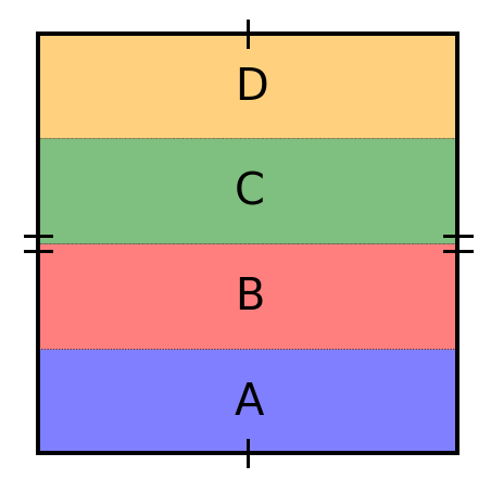
Figure 1: Our regions chosen for evaluating the topological entanglement entropy $S_{top}$ are cylinders on a torus. This can be represented as rectangles on a 2D plane with opposite sides identified.

$S_{top}$ is particularly valuable when considering generalizations of the random monitored circuit setup involving exotic measurements and phases. If the measurements are of stabilizers of a state with a distinguishable value of $S_{top}$, then an associated circuit phase may be readily distinguished. Taking the toric code $S_{top}$ as an example, the 4-term variant of $S_{top}$ (related to strong subadditivity) and 7-term version related above yield values of $1$ or $2$ respectively. This differs from the $0$ of simple product states, and also from the extensive scaling of states generically produced by Haar unitary dynamics [19].

Another guiding example is the 1D cluster state defined on an open chain [20]. Where the toric code realizes a genuine topological phase, the 1D cluster state is a symmetry-protected topological (SPT) state. In 1D such states are classified by the projective representations of the eponymous symmetry group acting on the boundary – that is to say, by the second group cohomology [45]. The associated phase in a random monitored quantum circuit also exhibits SPT behavior; in such a scenario, $S_{top}$ detects the edge degrees of freedom, again providing a value distinguishing the trivial phase from a more exotic SPT phase. The ancilla entanglement entropy also couples to these boundary degrees of freedom, facilitating the long-time storage of encoded edge qubits.

The cluster state behavior is particularly notable given the state’s relationship with measurement-based quantum computation (MBQC). MBQC is a well-known alternative to the gate model of quantum computation. Instead of evolving a state through a circuit and enacting entangling operations, one begins with a special entangled “resource state” and simulates a circuit via evolution with adaptive local measurements. A particular class of resource states are the so-called “graph states,” which are states defined on a graph, with qubits prepared in the $|{+}\rangle$ state on vertices, and edges denoting qubits between which controlled-Z operators are enacted. Equivalently, graph states can be said to be the joint eigenstate of the commuting operators $\sigma_{x}^{\alpha}\bigotimes\limits_{\beta\in N(\alpha)}\sigma_{z}^{\beta}$, where $\alpha,\beta$ label vertices and $N(\alpha)$ denote the graphical neighbors of $\alpha$. We will work with a slightly different convention, where a Hadamard is acted upon every qubit after this setup, exchanging the roles of the Pauli operators $X$ and $Z$.

The power of resource states is often attributable to underlying symmetries, whose presence reflect a kind of irreducible entanglement structure [46]. Cluster states, defined on graphs of regular lattices, exhibit such symmetries. The 1D cluster state, for example, features $\mathbb{Z}_{2}\times\mathbb{Z}_{2}$ global symmetry, the factors flipping spins on even/odd sites. This symmetry enables the state to act as a 1D wire, facilitating the teleportation of an encoded edge qubit by measurement [24]. Similarly, the 2D cluster state, enjoying an extensive number of subsystem $\mathbb{Z}_{2}$ line symmetries, belongs to a universal phase for MBQC [47].

The 1D cluster state was investigated in a random monitored quantum circuit context by Lavasani et al. [20]. In the spirit of the cluster state belonging to a nontrivial SPT class, their circuits preserve $\mathbb{Z}_{2}\times\mathbb{Z}_{2}$ symmetry. Their three-qubit unitaries, beyond belonging to the Clifford class that maps Pauli operators to other Paulis, furthermore conserves certain local parity operators. They found three distinct phases in their scenario, including a special “SPT” phase in addition to the usual volume-law and trivial entanglement phases. Notably, they also found that all phase transitions appear to belong to the same universality class, with correlation length critical exponents of $\nu\approx 4/3$ matching $(1+1)$D percolation theory.

This is curious; even though the phase transition recognizes that the SPT phase differs somehow from the trivial phase, the transition in itself does not reflect the difference in computational usefulness. In a sense, the transition between volume and trivial phases is “the same” as the transition between the volume and SPT phases. That is to say, the transition recognizes a difference in entanglement structure apparently disjoint from a possible accompanying computational transition.

The question, then, arises as to whether a transition in resource power distinct from percolation can arise in random monitored quantum circuits. We might be hopeful, since the 1D cluster state is not a universal resource, whereas its 2D and 3D counterparts feature novel qualities and more elaborate symmetry structure. Many other resource states belong to special SPT classes with distinguished global symmetries [25, 46, 24, 48, 49, 50], but an important characteristic of the 2D cluster state is the presence of additional subsystem symmetries [47]. Investigation of this additional find-grained symmetry has led to reveal the SPT phases which are universal for MBQC [47, 51, 52, 53]. Consideration of this also provides additional constraints on random monitored circuits, and inspires the setting of our work.

III $(2+1)$D Symmetric circuit

III.1 Setting

We study $(2+1)$D random monitored circuits with two different measurement types and draw from select unitary ensembles. Our system is defined periodically on a torus, and following the style of [20] our operations applied one at a time, rather than the more standard brick-pattern (see Fig. 2). At each time step we apply one of the following operations with their corresponding probabilities:

$$U p_{u},$$ 5-Qubit Clifford

$$M^{z} p^{z}_{M},$$ Local Z Measurement

$$M^{s} p^{s}_{M}.$$ Cluster Stabilizer Measurement

These probabilities sum to unity. After the operation is selected any system qubit is chosen with equal probability to be the center of the operation. If the $Z$-basis measurement is the operation, then the qubit is measured. For the 5-qubit unitary or cluster stabilizer measurement the qubit is chosen as the center around which either operation is applied in a “+”-shaped stencil, as depicted in Fig. 3.

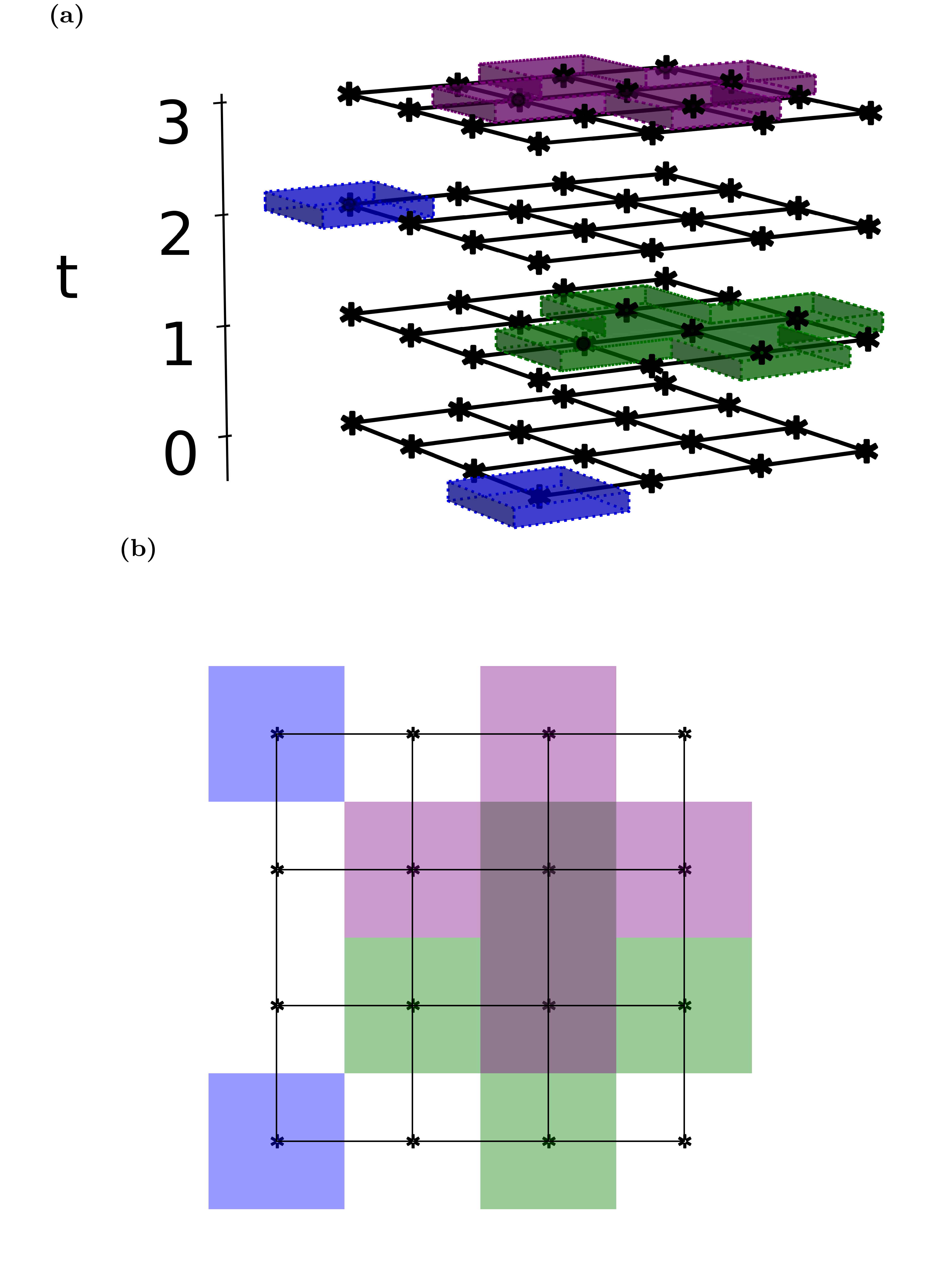
Figure 2: Example 3D (LABEL:fig:exa) and overhead view (LABEL:fig:exb) of the kind of circuits we consider. Two types of measurements are applied, one on a single site in the $Z$ basis and another in a “+” shape measuring a stabilizer of the 2D cluster state. 5-qubit unitaries are also applied in a “+” shape. One operation is applied every time step $t$.

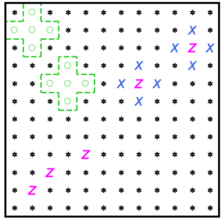
Figure 3: The three types of operations performed by our random circuits. Each symbol stands in for a qubit. On the lower left are local computational basis “Z” measurements. The upper right has measurements of 2D cluster state-like stabilizers. The upper left features 5-qubit Clifford unitaries.

We consider three ensembles of unitaries in our circuits. These ensembles are required to satisfy no symmetry requirement, a global symmetry requirement, and a subsystem symmetry requirement respectively, with associated groups $\mathds{I}\subset\mathbb{Z}_{2}\times\mathbb{Z}_{2}\subset\mathbb{Z}_{2}^{2L-1}$ for the 2D $L\times L$ square lattice (See the section 3.4 of Ref. [53] for an elucidation of the difference between the line symmetry $\mathbb{Z}_{2}^{2L-1}$ and the so-called cone symmetry $\mathbb{Z}_{2}^{2L}$). Recall that for more familiar settings of second-order phase transitions, such as the classical Ising model, the Hamiltonian possesses some symmetry that can be spontaneously broken, such as $\mathbb{Z}_{2}$. As the Hamiltonian generates dynamics, it follows that time evolution under it observes the same symmetry. We can similarly say that a class of circuit dynamics whose constituent unitaries all respect some symmetry group possesses that group as a symmetry.

A given circuit in our setting makes use of only one ensemble of unitaries. Including measurements, we have three phase diagrams for each ensemble, each with three probabilities. To access large system sizes via the stabilizer formalism (reviewed in Appendix A.1) [54, 55] all ensembles are subgroups of the 5-qubit Clifford group. As our primary interest is the entanglement structure of pure states at various times, we may safely neglect stabilizer signs and the concomitant computational complexities.

Our first ensemble consists of the entire 5-qubit Clifford group, the set of all unitaries normalizing 5-qubit Pauli operators, which we say possesses the trivial symmetry group $\mathds{I}$. The second ensemble is generated similarly, and comprised of symmetric 5-qubit Cliffords that respect the global $\mathbb{Z}_{2}\times\mathbb{Z}_{2}$ checkerboard symmetry enjoyed by the 2D cluster state on a torus. This is depicted in Fig. LABEL:fig:syma, and emulative of the symmetry considered in Ref. [20]. Their reduction to “+”-shaped stencils is shown in Fig. LABEL:fig:resa. Finally, the last ensemble has Cliffords respecting the $\mathbb{Z}^{2L-1}$ subsystem symmetries of the toric 2D cluster state. These symmetries are depicted in the top subfigures of Fig. LABEL:fig:symb, with their reduced stencils in Fig. LABEL:fig:resb. Although the former two ensembles are too large to store and generated “on the fly” as needed, the latter ensemble of unitaries is small enough to be generated and stored in its entirety. More details on generation are covered in Appendix A.2.

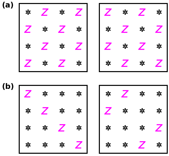
Figure 4: The global $\mathbb{Z}_{2}\times\mathbb{Z}_{2}$ “checkerboard” (Fig. LABEL:fig:syma) and subsystem $\mathbb{Z}^{\otimes 2L-1}_{2}$ “diagonal” (Fig. LABEL:fig:symb) symmetries respected by Clifford ensembles. The system here consists of $4\times 4$ qubits on a periodic lattice, making the diagonal symmetries wrap.

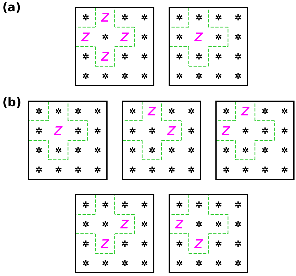
Figure 5: Local stencils of Pauli operators that a unitary applied on the center qubit must respect for the global “checkerboard” (Fig. LABEL:fig:resa) and “diagonal” subsystem (Fig. LABEL:fig:resb) symmetries. These are local reductions of the symmetries depicted in Fig. 4.

III.2 Numerical Methods

To reach large system sizes while still being able to describe highly entangled states we employ the stabilizer formalism [54, 55]. All unitaries used are accordingly necessarily of Clifford type. We have written our own C99 code capable of running several simulations in parallel with the aid of a Python wrapper. Most matrix manipulations are vectorized, with the binary bits of stabilizer matrices being stored in 256-bit integer vectors to permit rapid binary operations. As phase factors are of little interest for our study, we ignore them, saving on the traditional complications of determined measurement-outcomes.

We detect transitions using three diagnostics: the topological-, ancilla-, and dumbbell entanglement entropies ($S_{top}$, $S_{anc}$, and $S_{dumb}$) [38, 39, 40, 10, 56]. $S_{top}$ is our primary workhorse. We make use of the 7-term variant in Eq. 2 with regions defined as in Fig. 1 along quasi-1D cylinders. We have furthermore cross-checked our analysis with other geometries, such as diagonal subregions, as well as a more traditional “ring” setup. Appendix B.1, besides discussing the finer details of our implementation, also shows that the critical points and exponents match within numerical error for these other geometries. The ancilla entanglement entropy $S_{anc}$ has its value as a geometrically-independent comparative sanity check, and our implementation is discussed in Appendix B.2.

This question of geometry is relevant, due to the effect of so-called spurious topological entanglement entropy [56, 57], wherein subsystem symmetries may induce additional correlations that the topological entanglement entropy defined for special regions may be sensitive to. The dumbbell entanglement entropy [56], which is a diagnostic of subsystem symmetry, turns this inconvenience into a tool. We employ it to detect the transition in the case of pure measurement dynamics (i.e. when $p_{u}=0$), where neither the topological entanglement entropy nor the ancilla entanglement entropy are effective. The details are contained in Appendix B.3.

For our finite-size scaling analysis to retrieve details of our transitions we employ three different curve-fitting schemes. The first method, “Nearest,” seeks to make a hypothesized master curve connecting adjacent scaled points along the master curve as smooth as possible. The second, “Multilevel,” compares not with just the nearest scaled points, but all the nearest scaled points for all different system sizes. Finally, the last, “Polynomial,” is as the name suggests a high-order polynomial fit quantified by the residual. For sufficiently well-behaved data and enough datapoints the three typically agree, although the second would seem the most robust, while the last produces the smoothest plots. A more in-depth coverage of this topic is found in Appendix C.

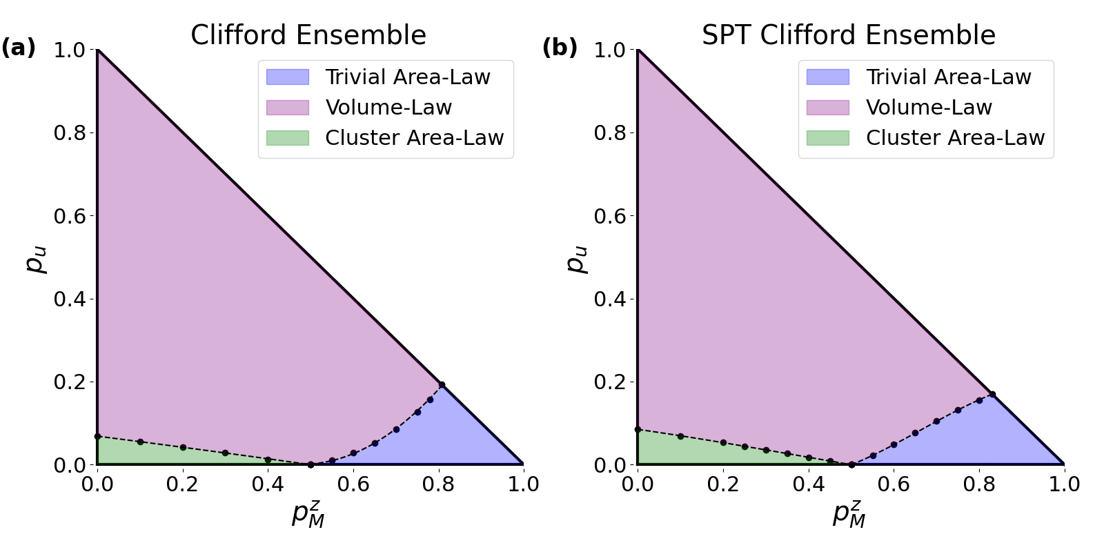
Figure 6: Phase diagrams for the unconstrained Clifford ensemble (LABEL:fig:regphase) and global symmetry-constrained (LABEL:fig:sptphase) ensembles in terms of the probabilities of applying 5-qubit Cliffords $p_{u}$ and computational basis $Z$ measurements $p_{M}^{z}$. Phase transitions occur at black dots, interpolations between which form the phase boundaries. Both diagrams are qualitatively similar, with small area-law entanglement regions due to the scrambling power of the 5-qubit Clifford ensembles.

III.3 Results

III.3.1 Unconstrained Clifford Group

Our unconstrained Clifford group refers to the group of all 5-qubit Cliffords, whose symmetry group is trivial. The entire phase landscape is shown in Fig. LABEL:fig:regphase. There are three phases: a trivial area-law phase, a cluster area-law phase, and one volume-law phase. As a consequence of 5-qubit Cliffords consisting primarily of entangling unitaries, the volume region is considerably larger than the other two.

The critical behavior along the $p_{M}^{s}=0$ line (where no cluster stabilizers are measured) is expected [7], and has been numerically shown [58] (with some prior controversy [59, 60]), to exhibit behavior akin to the 3D bond percolation transition. In particular, the correlation critical exponent is expected to take on the value $\nu\approx 0.88$. It is maybe not surprising that this critical behavior persists throughout the phase diagram – that is, even when we introduce cluster stabilizer measurements.

We observe such a similar critical exponent along the $p_{M}^{z}=0$ line. The data, along with the fitting landscape and the finite size scaling associated with the minimum thereof, is depicted in Fig. 7 below, where $\nu\approx 0.90$. This is not surprising for the reason that the essential phenomena seen in the one-operation-per-time-step scheme we employ do not differ from more standard maximally scrambling setup. In these latter setups, however, the unitary subgroup averaging property may be used to replace single-qubit measurements by another operator sharing the same locality as the applied unitaries. Specifically, since the Clifford unitary taking (in the Heisenberg picture) the operator $Z$ to the cluster state stabilizer $XXZXX$ belongs to the set of all 5-qubit Cliffords, it follows that we may heuristically exchange the roles of measuring either operator and expect qualitatively similar phenomena. It is important to note, however, that this argument cannot be applied in the SPT or SSPT case, as symmetry demands that all permitted unitaries take the $Z$ operator to itself.

We also include in this subsubsection analysis of the pure measurement dynamics, which, being in the limit where no unitaries are applied, is the same for all ensembles. The data is depicted in Fig. 8. Numerical collapse shows the critical point to be at about $p_{c}\approx 0.5$, which a duality argument similar to [20, 19] suggests should be exactly $p_{c}=0.5$. The critical exponent, meanwhile, is $\nu\approx 0.85$, which again matches $(2+1)$D percolation. Further investigation into the properties of this pure measurement critical phase are found in Appendix D. We thus have evidence that the criticality class is constant along all phase boundaries for this unconstrained class of unitaries.

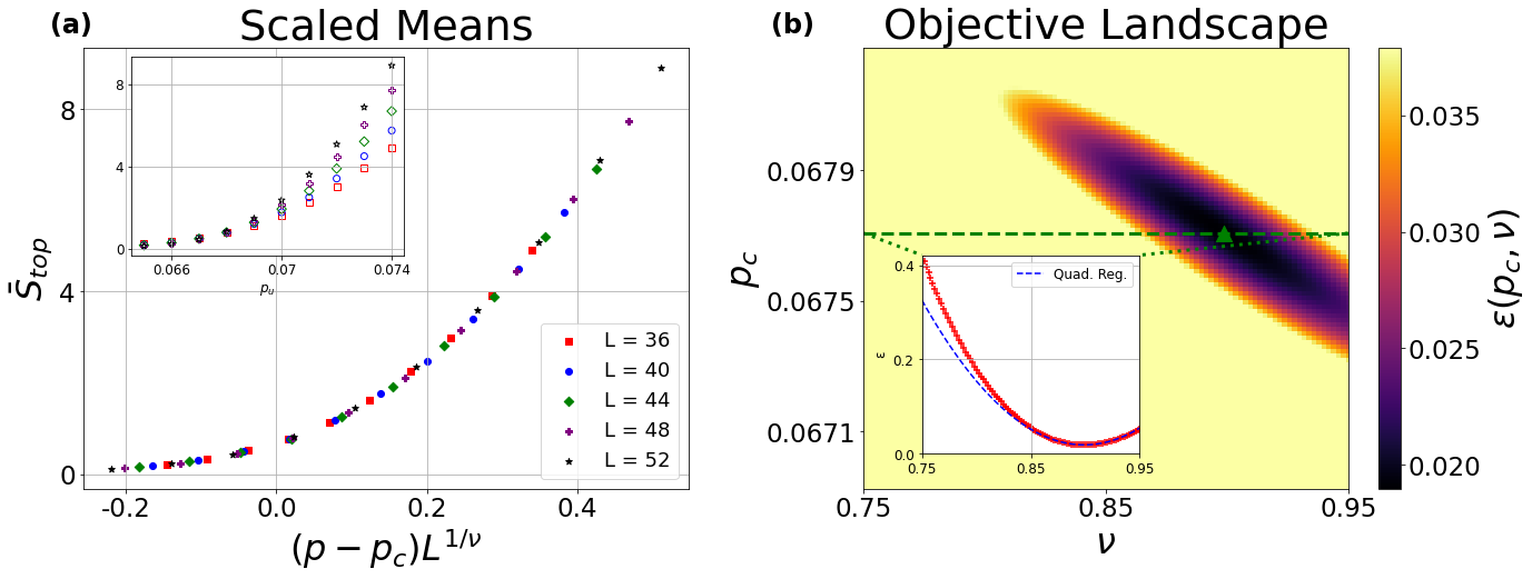
Figure 7: Data/analysis using the average 7-term topological entanglement entropy $\bar{S}_{top}$ with quasi-1D cylindrical geometry for the cluster-to-volume transition for the unconstrained Clifford ensemble. (LABEL:fig:7a): collapsed data as a function of the probability of applying a unitary operation $p_{u}$ (unscaled data inset). (LABEL:fig:7b): objective landscape for the collapse using a polynomial fitting method (slice at $p_{u}=p_{c}$ inset). The minimum is found at the critical point $p_{c}\approx 0.068$ and critical exponent $\nu\approx 0.90$.

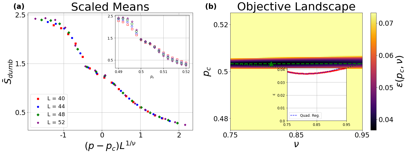
Figure 8: Data/analysis using the average dumbbell entanglement entropy $\bar{S}_{dumb}$ for pure measurement dynamics. No unitaries are employed, so this is the same for every ensemble. (LABEL:fig:8a): collapsed data as a function of the probability of performing a local computational basis measurement $p_{s}$ (unscaled data inset). (LABEL:fig:8b): objective landscape determining the collapse (slice at $p_{s}=p_{c}$ inset). The minimum is at critical point/exponent $p_{c}\approx 0.5$/$\nu\approx 0.84$.

III.3.2 SPT Clifford Group

The SPT Clifford group considered consists of all 5-qubit Cliffords that respect the $\mathbb{Z}_{2}\times\mathbb{Z}_{2}$ checkerboard symmetry group of the 2D cluster state. This is akin to a restriction placed on 3-qubit Cliffords on symmetric $(1+1)$D circuits, which has a phase characterized by measurements of 1D cluster state stabilizers [20]. The global symmetries in question preserved by 5-qubit unitaries are depicted in Fig. LABEL:fig:syma, with associated stencils in Fig. LABEL:fig:resa.

Our results in this case are similar to Ref. [20]. We find that although three distinct phases exist, the critical exponent remains close to that of $(2+1)$D percolation, with $\nu\approx 0.84$. The phase diagram, presented in Fig. LABEL:fig:sptphase, is quite similar to the unrestricted ensemble above. The primary visual difference is slight growth in the size of the trivial area-law phase, owing to the unitary ensemble considered being somewhat less entangling by virtue of imposed symmetry restrictions.

III.3.3 SSPT Clifford Group

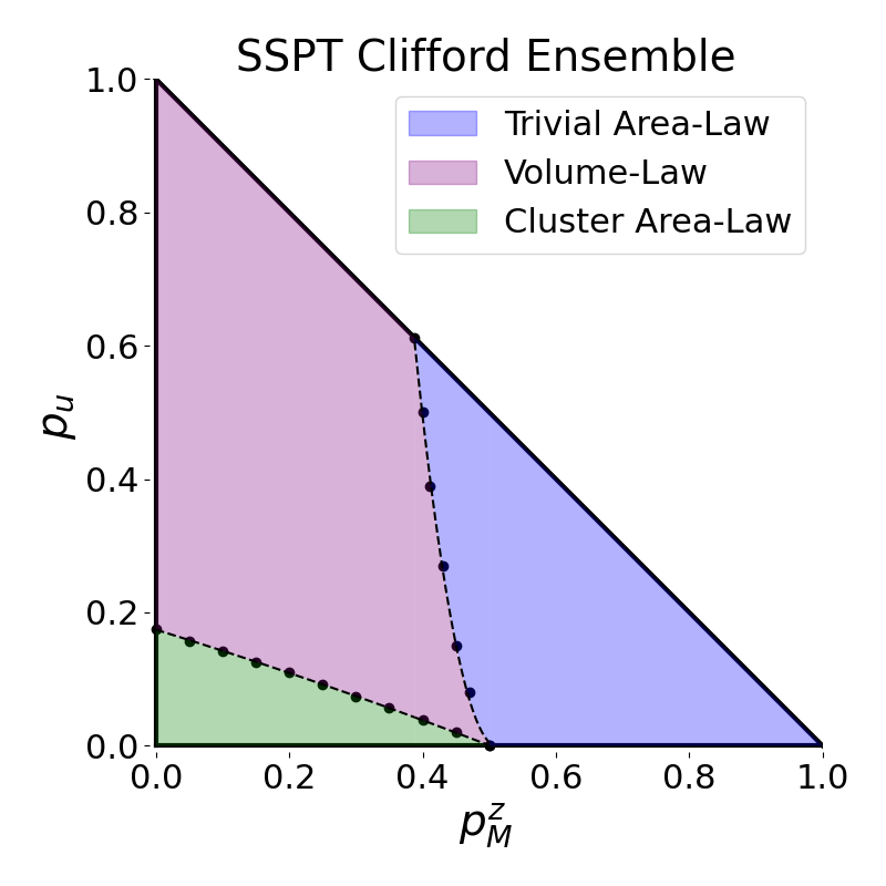
Figure 9: Phase diagram for the SSPT Clifford ensemble in terms of the probability of applying a 5-qubit unitary $p_{u}$ and a computational basis $Z$ measurement $p_{M}^{z}$. The three phases are separated by boundary lines determined by interpolating critical points obtained numerically at the black dots. Compared to Fig. LABEL:fig:regphase and Fig. LABEL:fig:sptphase, the trivial and cluster area-law regions are considerably larger, and the critical exponents generally differ.

The SSPT Clifford group is constituted by the 5-qubit Cliffords preserving the $\mathbb{Z}^{2L-1}_{2}$ line symmetries of the 2D cluster state. This includes, as a subgroup, the symmetries respected by the SPT ensemble, and so this constraint is strictly stronger. Examples of the line symmetries are depicted in Fig. LABEL:fig:symb, while the local stencils are shown in Fig. LABEL:fig:resb. For the 2D cluster state on open boundaries, as with global symmetry of the 1D cluster state, these symmetries act projectively on edge modes, and protect the boundary degeneracy [61]. Although our dynamics take place on the torus, we nevertheless preserve these symmetries, and hence expect to preserve certain properties of the resource.

The phase landscape is depicted in Fig. 9. The qualitative features of the three regions have noticeably changed compared to the previous two ensembles; the area-law regions have expanded considerably, owing to our constraints having made the unitaries considered less entangling. The trivial entanglement phase in particular has grown, as all permissible unitaries must preserve a Pauli $Z$ acting on the central qubit.

We find that the critical exponent along the $p^{z}_{M}=0$ line differs significantly from the percolation exponent. Through several diagnostics, and three separate fitting routines, we consistently find $\nu\approx 0.39$. Example data is depicted in Fig. 10 – more may be found in Appendix B.1. Comparable values of $\nu$ are found along the phase boundary, terminating at the $p_{u}=0,p^{z}_{M}=0.5$ measurement-only critical point. The volume-to-trivial-area-law transition for this ensemble is presented in terms of the ancilla entanglement in Fig. 11, with $\nu\approx 0.52$. Both critical exponents differ considerably from the $(2+1)$D percolation universality class with its characteristic $\nu\approx 0.87$.

We interpret these new exponents to reflect a shortfall of the previously-known percolation mapping, wherein all unitaries becomes impasses regardless of their original form. On one hand, the mapping is certainly justifiable for Haar-random unitaries, as the set of products of single-qubit unitaries constitutes a set of measure zero. For Clifford-random, and even for 1D $\mathbb{Z}_{2}\times\mathbb{Z}_{2}$-respecting Cliffords [20], this mapping still appears empirically justified, possibly because typical unitaries in these ensembles remain sufficiently entangling. For our final ensemble here, however, the large number of restrictions for the subsystem symmetries we have imposed – especially the requirement of preservation of the Pauli $Z$ on the center qubit – may make this simplification no longer applicable.

			Volume/Cluster Area			Volume/Trivial Area
Unitary Group			($p_{c},\nu$)			($p_{c},\nu$)
Clifford	$\mathds{I}$		$0.068\pm 0.001$	$0.90\pm 0.03$		$0.193\pm 0.005$	$0.85\pm 0.03$
SPT Clifford	$\mathbb{Z}_{2}\times\mathbb{Z}_{2}$		$0.084\pm 0.002$	$0.83\pm 0.03$		$0.170\pm 0.001$	$0.83\pm 0.05$
SSPT Clifford	$\mathbb{Z}_{2}^{2L-1}$		$0.176\pm 0.001$	$0.38\pm 0.05$		$0.612\pm 0.002$	$0.52\pm 0.06$

Table 1: Critical points $p_{c}$ and exponents $\nu$ along two phase boundaries. $p_{c}$ refers to the value of $p_{u}$ with $p_{M}^{z}=0$ for the volume/cluster area-law and $p_{M}^{z}=1.0-p_{u}$ for the volume/trivial area-law phase transitions respectively.

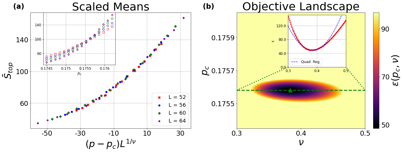
Figure 10: Data/analysis using the average 7-term topological entanglement entropy $\bar{S}_{top}$ with quasi-1D cylindrical geometry for the cluster-to-volume transition for the SSPT Clifford ensemble. (LABEL:fig:10a): collapsed data as a function of the probability of applying a unitary operation $p_{u}$ (unscaled data inset). (LABEL:fig:10a): objective landscape for the collapse using a polynomial fitting method (slice at $p_{u}=p_{c}$ inset). The minimum is found at the critical point $p_{c}\approx 0.176$ and critical exponent $\nu\approx 0.38$.

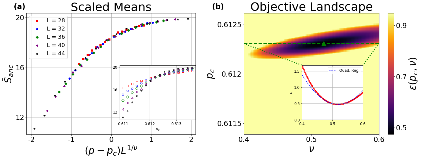
Figure 11: Data/analysis using the average ancilla entanglement entropy $S_{anc}$ for the volume-to-trivial-area-law transition. (LABEL:fig:11a): collapsed data as a function of the probability of applying a unitary operation $p_{u}$ (unscaled data inset). (LABEL:fig:11b): objective landscape determining collapse (slice at $p_{u}=p_{s}$ inset). The minimum is at critical point/exponent $p_{c}\approx 0.612$/$\nu\approx 0.52$.

IV Discussion

We have studied the interplay between a hierarchy of increasingly restrictive symmetries and the phases observed in $(2+1)$D random monitored quantum circuits. We have shown that, in contrast to the SPT case in (1+1)D [20], the cluster area-law phase of a random monitored quantum circuit for a subsystem-symmetry respecting ensemble of Clifford unitaries features a different universality class than unrestricted dynamics in $(2+1)$D. Our results are summarized in Table 1. The volume-to-cluster-area-law transition has a critical exponent of $\nu\approx 0.38$, and the volume-to-trivial-area-law transition has $\nu\approx 0.52$. These values are quite different from $\nu\approx 0.88$ for globally-symmetric and unrestricted 5-qubit Cliffords. The (1+1)D SPT case is analogous to the global symmetry considered here, where the transitions all appear to remain within the percolation universality class. This suggests that the presence of subsystem symmetry is fundamentally altering certain critical dynamics.

It may be useful to compare our setting with other hierarchies of symmetries in phase transitions. Recall that our (2+1)D Clifford, SPT Clifford, and SSPT Clifford circuits feature symmetry groups $\mathds{I}\subset\mathbb{Z}_{2}\times\mathbb{Z}_{2}\subset\mathbb{Z}_{2}^{2L-1}$ respectively. The $O(N)$ classical spin model, whose Hamiltonian is $H=J\sum_{\langle\alpha,\beta\rangle}\mathbf{S}_{\alpha}\cdot\mathbf{S}_{\beta}$ for the $N$-component spin, contains the Ising, XY, and Heisenberg models as special cases, with associated symmetry groups $\mathbb{Z}_{2}\subset O(2)\subset O(3)$ respectively. The critical phenomena of these models have been studied extensively, and the critical exponent $\nu$ is known to increase with $N$ in this hierarchy – approximately equal to $0.63,0.67,$ and $0.70$ respectively in the spatial dimension $d_{s}=3$ [62, 63, 64]. It is believed that this trend is true regardless of whether the spin is treated classically or quantumly. It is also known that the one-loop analysis of the fixed point in more general spatial dimension $d_{s}=4-\epsilon$ theory yields the following expression for the exponent for general $N$:

$$\frac{1}{\nu}=2-\frac{N+2}{N+8}\epsilon.$$

This suggests that $\nu$ generally increases with $N$ [65].

In contrast, for our hierarchy of lattice symmetries, $\nu$ is about the same for $\mathds{I}$ and $\mathbb{Z}_{2}\times\mathbb{Z}_{2}$ ($0.83$ and $0.85$), and decreases for the subsystem symmetry to $0.38$. This is the opposite trend. It might be fruitful to investigate the relationship between hierarchies of symmetries and critical exponents in broader contexts.

Lastly, given the well-known kinship of SPT and SSPT symmetries and measurement-based quantum computation (MBQC), understanding if this difference in transition characteristics relates to a differentiation of computational power is also a matter of interest, and will be the subject of future investigation. It is worth noting that, just as for the full Clifford group, the critical exponents observed for the SSPT ensemble violate the Harris criterion [66]. This criterion states that local disorder is a relevant perturbation (in the renormalization group sense) when the correlation length critical exponent $\nu<2/d_{s}$, where $d_{s}$ is the spatial dimension. As recent work has investigated the effect disorder has on the measurement-induced phase transition [67, 68], investigating parallels between the effects of such disorder and potential counterparts in MBQC might also be a potentially interesting direction.

V Acknowledgements

This work was supported by the National Science Foundation STAQ Project (PHY-1818914, PHY-2325080) and PHY-2310567. We would like to thank the UNM Center for Advanced Research Computing, supported in part by the National Science Foundation, for providing the research computing resources used in this work.

Appendix A Simulation Methods

A.1 Stabilizer Formalism

One possible pitfall of using entanglement entropies to probe the measurement-induced phase transition is the drifting of the critical parameter $p_{c}$ for small system sizes [69]. Coupled with other finite size effects, it is often necessary to simulate large numbers of qubits to attain a quantitative hold on properties of the transition, especially for higher dimensions [58].

To reach these larger system sizes we employ stabilizer machinery [54, 55]. This well-known formalism tracks the quantum state $\rho$ in terms of its stabilizers $S(\rho)$, which are the group of operators of which the state is a $+1$ eigenstate. $S(\rho)$ may be conveniently handled by looking at its generators. For the standard setting of qubits it is often the case of interest that $S(\rho)$ is an Abelian subgroup of the Pauli group of tensor products of the single-qubit operators $\{I,X,Y,Z\}$, including an overall phase. In this case the generators themselves are Paulis with phases, and are computationally amiable. For this reason, Pauli stabilizer states are simply referred to as the “stabilizer states” for short.

The $n$-qubit Pauli operators constituting the stabilizers of a stabilizer state may be represented (up to phase) by a string of $2n$ binary elements. By convention, the bits of such a string correspond to the presence or absence of an $X$ or $Z$ for a particular qubit, with a $Y$ understood by the presence of both. Often all $X$ bits are grouped together, followed by the $Z$ bits. Hence, the $2$-qubit operators $X_{1}X_{2}$, $Z_{1}X_{2}$, $I_{1}X_{2}$, and $Y_{1}Z_{2}$ may be represented by the strings $1100$, $0110$, $0100$, and $1011$ respectively. With this technology, the $n$ generators of a Pauli stabilizer state’s stabilizer group may thus be represented by a $n\times 2n$ binary matrix. This results in considerable savings on space complexity compared to the naive representation of generic states.

One typically wishes not for some quantum state by itself, but rather that state as the input or output of some circuit consisting of unitary actions and measurements. Stabilizer states typically cease to be such under generic operations. However, in the case of measurements of Pauli operators and a special subset of unitaries known as Clifford unitaries, stabilizer states are mapped to stabilizer states. Restriction of circuit elements to these operations permits efficient simulation of a state’s evolution [54].

Clifford unitaries are the normalizer $\mathcal{N}(\mathcal{P})$ of the set of Pauli products $\mathcal{P}$, i.e. the subset of unitaries $U\in\mathcal{N}(\mathcal{P})\subset U(2^{n})$ such that $U^{-1}\mathcal{P}U=\mathcal{P}$. Limiting one’s attention to Pauli products consisting only of one, two, three, etc. non-identity factors, one speaks of $1$-, $2$-, $3$-, etc. Clifford operators. When a Pauli group of symmetries is enforced on the system, the set of allowed Cliffords is further reduced by the requirement that they belong to the centralizer of that Pauli subgroup. The action of Clifford unitaries on a stabilizer state can be understood via their Heisenberg representation action on the state’s stabilizer group. Representing that group’s generators via binary matrices, Cliffords correspond to symplectic operators over $\mathbb{Z}_{2}$. Hence, not only are stabilizer states efficiently expressible, but so too are the natural unitary operations upon them.

We now turn to measurements. The measurement of an operator results in a projection of the state. As Pauli operators only have the two eigenvalues $\pm 1$, and since they square to the identity, this projection takes on the form $\Pi^{\pm}_{P}=\tfrac{1}{2}(\mathds{I}\pm P)$, where $P$ is the Pauli operator being measured. The density operator of a stabilizer state $\rho$ itself may itself be represented as a product of the projectors corresponding to the generators of its stabilizer group $S(\rho)$ – this is a consequence of basic representation theory. We write the stabilizer state operator as

$$\rho=\prod\limits_{i=1}^{n}\Pi_{P_{i}}$$

The action of $\Pi^{\pm}_{P}$ on the density matrix $\rho$ of a state can be understood by looking at its conjugate action on another projector $\Pi_{P^{\prime}}$:

$$\Pi^{\pm_{1}}_{P}\Pi_{P^{\prime}}\Pi^{\pm_{1}}_{P} =\frac{\mathds{I}\pm_{1}P}{2}\frac{\mathds{I}+P^{\prime}}{2}\frac{\mathds{I}\pm_{1}P}{2},$$

$$=\frac{2(\mathds{I}\pm_{1}P)+(P^{\prime}\pm_{1}(PP^{\prime}+P^{\prime}P)+PP^{\prime}P)}{8}.$$

Two Paulis either commutate or anticommutate with one another. When they commutate, the above product becomes $\Pi_{P^{\prime}}\Pi^{\pm_{1}}_{P}$. When they anticommutate, the result is $\tfrac{1}{2}\Pi^{\pm_{1}}_{P}$. As the stabilizer group is Abelian, the $\Pi_{P_{i}}$ factors of $\rho$ may be freely ordered. One may hence group all the $P_{i}$s commutating with $P$ at the beginning, and move all those that anticommutate to the end. Let the generators commuting with $P$ be $\{R_{i}\}$ and those anticommutating be $\{Q_{i}\}$. Since any two $Q_{i}$s commutate with each other, the identity $\Pi_{Q_{i}}\Pi_{Q_{j}}=\Pi_{Q_{i}Q_{j}}\Pi_{Q_{i}}$ is satisfied. The product of the anticommutating generators may be written

$$\prod\limits_{i=1}^{m}\Pi_{Q_{i}} =\prod\limits_{i=1}^{m-1}\Pi_{Q_{1}Q_{i+1}}\Pi_{Q_{1}}.$$

The double products $Q_{i}Q_{j}$ commutate with $P$, and so may be absorbed into the commutating generators $R_{i}$. There is now only a single generator anticommutating with $P$. The action of $\Pi^{\pm}_{P}$ on $\rho$ can thus be written

$$\Pi^{\pm}_{P}\rho\Pi^{\pm}_{P} =\Pi^{\pm}_{P}\left(\prod\limits_{i=1}^{n}\Pi_{P_{i}}\right)\Pi^{\pm}_{P},$$

$$=\Pi^{\pm}_{P}\left(\prod\limits_{i}R_{i}\right)\Pi_{Q_{1}}\Pi^{\pm}_{P},$$

$$=\left(\prod\limits_{i}R_{i}\right)\Pi^{\pm}_{P}\Pi_{Q_{1}}\Pi^{\pm}_{P},$$

$$=\left(\prod\limits_{i}R_{i}\right)\Pi_{\pm P},$$

Our new list of stabilizers includes all the old commutating Paulis, all the old anticommutating Paulis (except $Q_{1}$) multiplied by $Q_{1}$, and the measured Pauli $P$ (replacing $Q_{1}$). A shorter explanation proceeds along the following logic. One first observes that $\rho$ may be represented using any choice of generators of $S(\rho)$. With this freedom, all anticommutating generators except for $Q_{1}$ can be replaced by $Q_{i}Q_{1}$. Then, in the expansion by projections one readily sees that applying $\Pi^{\pm}_{P}$ to the state has the effect of replacing the $Q_{1}$ projector with itself. As a whole, the algorithm can be described like so: if a measured operator $P$ anticommutates with some generators of the stabilize group of a state, replace one of the anticommutating generators $Q_{1}$ with $P$, then replace all other anticommutating $Q_{i}$ with $Q_{1}Q_{i}$.

We have ignored phases in this explanation, as they are not important for our purposes, however they introduce extra complications, even moreso when $P$ commutates with $S(\rho)$. Where the anticommutating case corresponds to a nondeterministic measurement, the commuting case represents a deterministic measurement. In this case, extra matrix manipulations must be performed to determine the sign of the deterministic measurement. The ensuing complications may be ameliorated by more thoughtful implementations [55, 70].

The advantage of the stabilizer formalism is twofold: reduced space complexity, and access to a class of highly entangled states. A general $n$-qubit wave function naively requires $\mathcal{O}(2^{n})$ numbers, and quickly becomes unfeasible to work with. Tensor approximations, meanwhile, effectively model the low-entanglement area-law phase, but fail in the volume phase and near the critical point. Qubit stabilizers require only $\mathcal{O}(n^{2})$ binaries, and are hardly less tractable in the volume-law phase than in the area. They therefore present an efficient probe of characteristics of measurement-induced phase transitions, provided our purposes are met by the limited stabilizer polytope of Hilbert space we are constrained to.

Our code stores the binary string corresponding to a given Pauli in chunks, with each chunk being a 256-bit integer vector. On somewhat more modern architectures, these vectors could be increased in size. This vectorization makes various operations, such as the calculating the product of two Paulis, quite fast, particularly since our purposes are agnostic to phases. Further improvements could be made, such as implementing advanced rank-calculation algorithms for finite fields instead of employing binary Gaussian elimination [71].

A.2 Unitary Generation

To simulate our random monitored circuits we must know how to implement the gates and measurements of interest. For measurements, this is simple. We only employ computational basis $Z$ measurements and 2D cluster state “+”-shaped stabilizer measurements (see Fig. 3). Carrying out these measurements in the stabilizer formalism is particularly easy, as our purposes are unconcerned with stabilizer phase.

For our three phase diagrams our gates are drawn from three corresponding unitary ensembles: unconstrained-, SPT-, and SSPT 5-qubit Cliffords. This poses a predicament, as the set of all 5-qubit Cliffords poses a prohibitive space requirement. The set of $n$-qubit Cliffords may be generated recursively given the set of $n-1$ qubit Cliffords via a well-known scheme [9]. At each step, one randomly selects an $n-1$ qubit Clifford and two anticommutating Pauli strings corresponding to what the $X$ and $Z$ operators map to for the newest qubit. Ignoring a phase, this amounts to $4^{k+1}-1$ possibilities for the first choice, and $4^{k}$ for the second. The number of unsigned $n$-qubit Cliffords may be obtained via induction:

$$\text{\# }n\text{-qubit Cliffords}=2^{n^{2}}\prod_{i=1}^{n}\left(2^{2(i+1)}-1\right).$$ (3)

This evaluates to $6,720,1451520,47377612800,$ and
$24815256521932800$ for $n=1,2,3,4,5$ qubits respectively. If each is naively represented by $2n\times 2n$ binary numbers, this corresponds to $24,11520,52254720,3032167219200,$ and
$2481525652193280000$ bits respectively, amounting to around $3b,1KB,7MB,380TB,300PB$ of space. Frontier currently boasts $700$ petabytes of storage capacity [72], so this is not beyond the scope of modern computational prowess, but a more parsimonious usage of resources would be preferable

A satisfactory approach we have found generates the unconstrained Clifford and globally-constrained SPT Clifford ensembles “on the fly” using the standard recursion algorithm. We store all 3-qubit Cliffords, which may be generated very quickly. By randomly selecting anticommutating 4-qubit and 5-qubit Paulis, which have also been computed and stored in advance, we then generate random 4-qubit and then 5-qubit Cliffords. For the SPT Clifford ensemble, additional checks are performed to ensure that the resultant unitary is adequate – this process may be sped up by thoughtful implementation optimizations.

The SSPT Clifford ensemble is small enough to be collected, stored, and sampled from as needed. The set of all 5-qubit Cliffords can be searched through by generating it in small enough chunks to be stored and have symmetry conditions checked. This procedure is readily parallelized. We have found that a better (also parallelizable) method starts by generating the small number of acceptable “Z” columns of such unitaries, then complete the remainder by generating and checking all compatible “X” columns. This last method may be realized in a matter of hours even with Python.

Appendix B Diagnostics

In the conventional classification of ground states, SPT states are short-range entangled states from the strict topological perspective [45]. This is to say that a shallow local circuit is able to transform them into product states with trivial entanglement. What defines symmetry-protected classes is that any such local circuit necessarily violates some natural symmetry. The requirement of this symmetry makes such a transition nontrivial, thus it is said that the symmetry eponymously protects the phase thus defined. It is not usually difficult to distinguish SPT states from volume-law states; most diagnostics distinguishing any area-law behavior from volume-law suffice. Distinguishing SPT area-law entanglement phases from trivial area-law phases, however, is more challenging. Furthermore, trying to identify strong SSPT states like the 2D cluster state – which are not genuinely global SPT states (see [73] for a more detailed explanation) – is an even more elusive task.

This section covers the three primary diagnostics we employ: the topological-, ancilla-, and dumbbell entanglement entropies. The first two consistently distinguish the cluster area-law phase from the volume phase, but do not distinguish between other area-law phases. The dumbbell entanglement entropy (see Fig. 12) successfully discriminates them, but is numerically less robust.

B.1 Topological Entanglement Entropy

The ground states of a large class of gapped 2D systems generically feature area-law behavior. A subregion $R$’s entanglement entropy with respect the rest of the system follows $S_{R}\sim c|\partial R|-\Gamma$. Here $|\partial R|$ is the area-law contribution, while $\Gamma$ represents subleading corrections encoding long-range correlations. For systems whose far-infrared behavior is well-described by topological quantum field theories $\Gamma=\log\mathcal{D}$, where $\mathcal{D}$ is the total quantum dimension of the effective theory. Extraction of $\Gamma$, which nicely characterizes the quantum phase in a single number, is typically carried out through clever combinations of entanglement entropies of varying regions; this is the topological entanglement entropy $S_{top}$ [38, 39].

The precise form comes in several varieties, possessing different numbers of terms and reflecting different geometries. The 2D cluster state has zero topological entanglement entropy for most conventional geometries, a property that is expected to be shared by a cluster area-law phase of our random monitored circuits. Nevertheless, variants of this quantity can still be used as an order parameter, since volume phase states will typically take on an extensive value.

Our primary analysis uses the 7-term variant of $S_{top}$, which is related to the tripartite mutual information (Eq. 2) [44]. Our geometry, meanwhile, is defined in terms of cylinders embedded in a torus, as shown in Fig. 1. Other natural geometries (inset in Fig. 13) yield results quantitatively similar to those covered in the main text. A key result of our simulations is the appearance of a new universality class for the transition between the SSPT Clifford volume-law phase and the cluster area-law phase. As an example of this agreement, Figs. 14 and 15 both illustrate, for the SSPT Clifford ensemble along the $p_{z}=0.0$ line, the analysis and collapse of $S_{top}$ using standard “ring” and diagonally-directed quasi-1D geometries. The critical point is, as for Fig. 10 in the main text, found to be $p_{c}\approx 0.176$ uniformly, while the critical exponent $\nu$ varies from $0.387$ to $0.406$.

Our sampling method is as follows. We first wait for a given instance of the circuit to reach a sort of steady state. This happens when the entanglement growth plateaus, which happens before some fraction of $L^{4}$ (we take that fraction to be $1/4$ for concreteness). Then, we sample $S_{top}$ every $L^{2}$ time steps, until time $\mathcal{O}(L^{4}$), at which point we start an entirely new circuit again from scratch with a fresh product state input. The sampling frequency is safely uncorrelated far away from the critical point, but as the critical point is approached the correlation time formally diverges. Nevertheless, we have found that the resultant statistical compromisation has an effect negligible compared to the effects of the accompanying growth of the statistical dispersion of the order parameter distribution of $S_{top}$. Our typical number of sample circuits depends on the system size, but varies from thousands to tends of thousands for smaller and larger systems respectively.

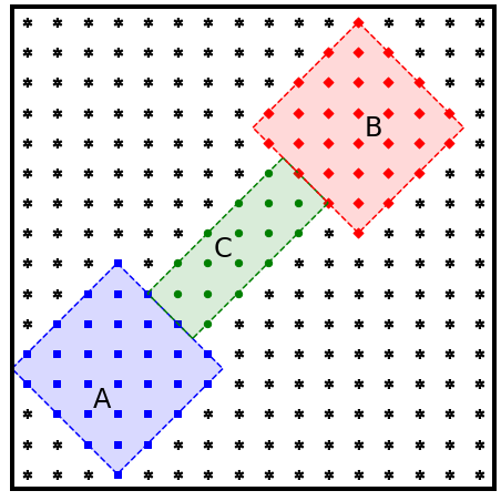
Figure 12: Example regions defined for the dumbbell entanglement entropy. In this work it is the tripartite mutual information of the heads conditioned on the handle, which is oriented along the direction of subsystem symmetries of the 2D cluster state.

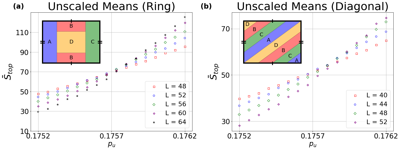
Figure 13: Unscaled data for 7-term average topological entanglement entropy $\bar{S}_{top}$ for the SSPT Clifford ensemble with $p_{M}^{z}=0$ as a function of the probability of applying a unitary operation $p_{u}$ for the standard “ring” geometry (LABEL:fig:unsclextraa) and “diagonal” geometry (LABEL:fig:unsclextrab) oriented along the direction of subsystem symmetry (geometries inset). Analysis of this data is shown in Figs. 14 and 15 respectively.

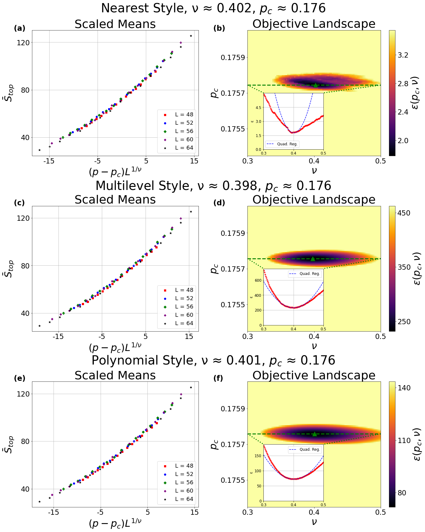
Figure 14: Analysis using the standard “ring” geometry. Data of the average 7-term topological entanglement entropy $\bar{S}_{top}$ for the SSPT Clifford ensemble is depicted with $p_{M}^{z}=0$ for the cluster-to-volume transition. (LABEL:fig:subregab), (LABEL:fig:subregcd), and (LABEL:fig:subregef) all illustrate collapse/objective landscapes (LABEL:fig:subregace/LABEL:fig:subregbdf) using three different fitting methods.

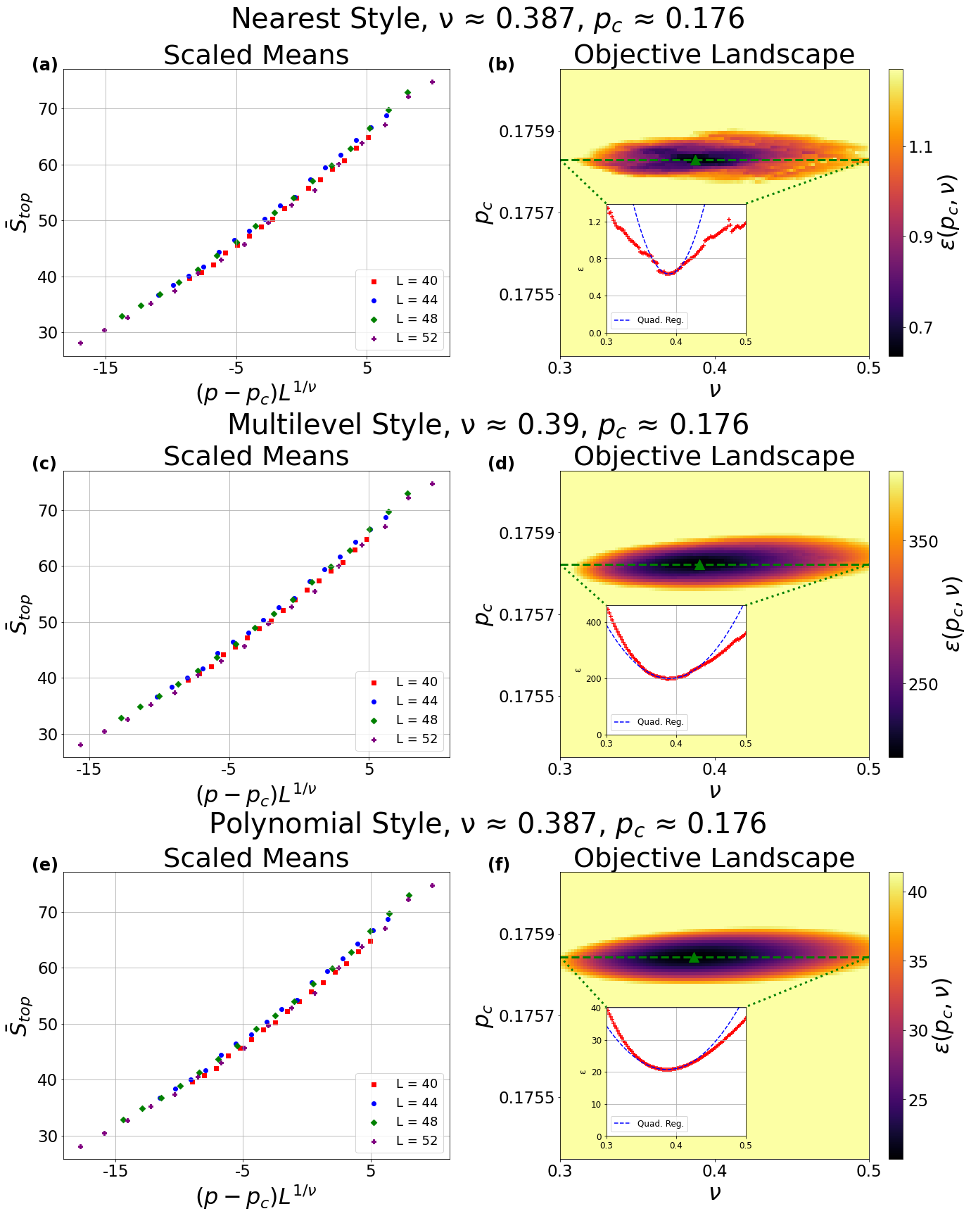
Figure 15: Analysis using the “diagonal” geometry. Data of the average 7-term topological entanglement entropy $\bar{S}_{top}$ for the SSPT Clifford ensemble is depicted with $p_{M}^{z}=0$ for the cluster-to-volume transition. (LABEL:fig:subdiagab), (LABEL:fig:subdiagcd), and (LABEL:fig:subdiagef) all depict collapse (LABEL:fig:subdiagace) and objective landscapes (LABEL:fig:subdiagbdf) (with inset slices) using our three fitting methods.

B.2 Ancilla Entanglement Entropy

One element underlying the stability of the volume phase of random monitored circuits is the notion of scrambling. Provided that the measurement rate is not too great, information about the initial state is, after some initial mixing time, encoded in long-range correlations that local measurements cannot efficiently probe. The ancilla entanglement entropy $S_{anc}$ takes advantage of this phenomenon [40, 10]. It is a measure of how much information about a probe entangled with the system (size $N$) remains encoded at a time $t$. Quantitatively, $S_{anc}$ is the von Neumann entropy of a probe entangled with the system:

$$S_{anc} =S_{vN}(\rho_{anc}),$$

where $\rho_{anc}$ is the state operator of the ancilla system. As with most probes, this must be evaluated for an individual trajectory, then averaged over measurement outcomes and circuit realizations to yield the diagnostic $\bar{S}_{anc}$.

As long as a few physical qubits have not been measured, some nonlocal correlations will survive between the system and the ancilla, and thus the von Neumann entanglement will be nonzero. Deep in the area-law phase, where measurements with probability $p$ are frequent, we can estimate the probability of survival like so. First, one assumes that at every time step each qubit has an independent probability $p$ of being measured. Then, the probability of any one qubit remaining unmeasured is the compliment of the probability that all qubits have been measured at some point in the past at a given time step. This probability is a power of the probability that any particular qubit has been measured at least once, which is the compliment of the probability that it’s never been measured at time $t$ – $(1-p)^{t}$. We can therefore write the survival probability of a probe’s information as $P\sim 1-(1-(1-p)^{t})^{\mathcal{O}(N)}$. This entails $\tau\sim\mathcal{O}(N)$ for large $t$ and $N$. Meanwhile, volume phase information is destroyed by the very rare event of an extensive number of measurements. For small $p$, this happens with probability $\sim p^{\mathcal{O}(N)}$, implying the survival probability $(1-p^{\mathcal{O}(N)})^{t}$ and lifetime $\tau\sim\exp(N)$. Evaluating the entanglement at sufficiently large $t$ effectively distinguishes these two behaviors.

Similar to the topological entanglement entropy, the ancilla entanglement entropy takes on a value tending towards $0$ in the cluster area-law phase of our circuits. That is to say, $S_{anc}$ does not differentiate it from the trivial area-law phase. But equally similarly, this suffices to distinguish the cluster area-law phase from the volume-law phase. This quantity may accordingly be used to probe transition throughout most of the phase diagram.

Our implementation is as follows. Before starting the circuit properly, we entangle $20$ ancillae by running a scrambling circuit for time $T=\mathcal{O}(L^{4})$, with the 5-Clifford unitaries enacted on any arbitrary five qubits (either ancilla or system), regardless of spatial separation. Then, we sample the entanglement between the ancilla and the system after $\mathcal{O}(L^{4})$ time steps. Immediately after scrambling, the entanglement is on order of $20$, and deep in the volume-law phase this value is retained for long periods of time. In the area-law phases, meanwhile, the entanglement drops quickly to zero. At criticality, a constant fraction of the original entanglement is retained in the thermodynamic limit, with the specific factor depending on when the entanglement is sampled.

Because of the initial mixing time, and since $S_{anc}$ is only really sampled once per circuit run, analysis of $S_{anc}$ requires more simulation time. It makes up for this defect by being formally less noisy in spite of this defect. Typical sample sizes ranges from high hundreds for the largest systems to high thousands for smaller ones.

B.3 Dumbbell Entanglement Entropy

While the topological entanglement entropy succeeds in distilling the topological essence of many nice models down to a single number, so-called “spurious” contributions can arise in systems exhibiting long-range string order [56, 57]. Though this fact spoils elegant theoretical models, its existence can be used as a diagnostic of the presence of SPT and SSPT effects. The dumbbell entanglement entropy $S_{dumb}$ [56] is a construction taking advantage of this fact. For this work we define it as the 7-term tripartite mutual information as in Eq. 2, rather than the conditional mutual information of [56]. As opposed to the more standard geometries used for $S_{top}$, the dumbbell entanglement entropy $S_{dumb}$ is so named for using regions forming dumbbell with the handle directed along a line of string symmetry (see Fig. 12).

We make use of this quantity in this work to distinguish the cluster area-law phase, exhibiting subsystem symmetry, from the trivial area-law phase generated by an excess of local computational basis measurements. While it succeeds in discriminating between the two behaviors, in practice it is less robust at its job than the topological- or ancilla entanglement entropies covered above. The defects in the curve (seen in Fig. 8) become more prominent near criticality, and capriciously depend on the size of the “head” and “handle.”

$S_{dumb}$ is sampled similarly to $S_{top}$ as described in Sec. B.1. We begin sampling at $t=\tfrac{1}{4}L^{2}$, and sample every $L^{2}$ timesteps, starting another circuit from scratch at $t=L^{4}$. This sampling frequency produces data sufficiently uncorrelated away from the critical point, but near the critical point the correlation time diverges along with the correlation length. Nevertheless, the statistical influence of this fact appears negligible compared to the growth of the spread of the order parameter distribution of $S_{dumb}$. Typical sample sizes range from thousands to tens of thousands for larger and smaller systems respectively.

Appendix C Fitting Methods

Although our presented data is analyzed using a single fitting method, we apply three different techniques as a check on our finite-size scaling analysis. We refer to them as “Nearest,” “Multilevel,” and “Polynomial” styles respectively. All take as input the critical parameters $(p_{c},\nu,\gamma)$, which scale the data as $(p,\Delta)\to((p-p_{c})L^{1/\nu},\Delta L^{-\gamma})$. Although we have included the extensive exponent $\gamma$ here, we have found that this is within margin of error $0$ in practice. It is therefore set to be exactly $0$ in all figures in this work.

For the “Nearest” style, we order the scaled data following $(p-p_{c})L^{1/\nu}$. A linear regression is performed for all interior points using their immediate neighbors, regardless of system size, and the goodness of fit for the whole curve is the sum of the goodness of fits for these individual regressions. This heuristically has the effect of favoring input parameters producing a curve that is locally as smooth as possible.

The second technique, “Multilevel,” is similar to the first. However, for each individual point, we look at each system size greater than that of the point, and then select neighbors from those to perform a regression. The objective function is the sum of the goodness of fit for each point for each system size larger than the size that point belongs to. The intuition underlying this method is that it favors input parameters specifying a curve as smooth as possible with respect to the samples coming from larger systems, which hypothetically suffer less from finite size effects.

The final “Polynomial” style is a simple polynomial regression on the entirety of the scaled data. Though crude, the output of this method produces smooth landscapes whose minima do not deviate significantly from the prior two methods, provided that the data is well-sampled and smooth. Eighth order polynomials have proven sufficient for our purposes; higher orders suffer from overfitting, while lower orders fail to capture the master curve’s contouration.

All figures in the main text employ the “polynomial” method. However, as shown in Fig. 14 and Fig. 15, all three methods are typically in good agreement.

Appendix D Behavior at Pure Measurement Critical Point

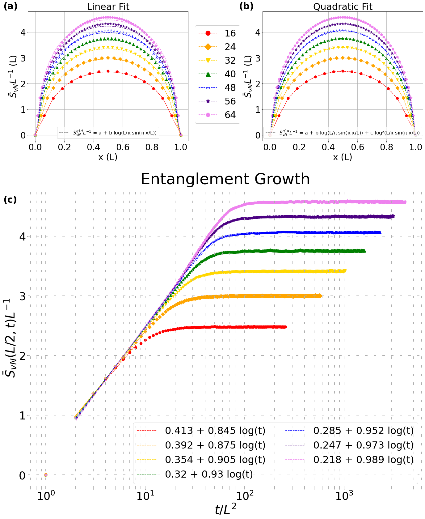
Figure 16: Plots of the scaled entanglement versus system length for linear (LABEL:fig:subentgrowtha) and quadratic (LABEL:fig:subentgrowthb) regressions, and half-system entanglement growth versus time (LABEL:fig:subentgrowthc). Colors/shapes refer to the same system sizes across all figures. The linear fit works well for small $L$, but consistently deviates for larger sizes, while the quadratic fit continues well. Meanwhile, the regression coefficients for the growth over time slowly vary with $L$.

For $(1+1)$D systems at criticality it is well-known that the entanglement entropy of a contiguous section (size $l$) of the system (size $L$) often features entanglement entropy scaling as

$$S_{1D}(l)=\text{Const.}+\tfrac{c}{6}\log\left(\tfrac{L}{\pi}\sin(\tfrac{\pi l}{L})\right),$$ (4)

where $c$ is the central charge of the associated conformal field theory [74, 75]. The entanglement entropy of a region of set size (say, half the system), meanwhile, grows logarithmically in time $S_{1D}(t)=a+b\log(t)$.

In 2D translationally invariant systems it is expected that spiritually similar expressions continue to hold, provided that quasi-1D sections of the system (such as cylindrical sections of a torus) are chosen. Furthermore, while the critical properties of random monitored quantum circuits do not precisely match the phenomenology of more conventional phase transitions, similar relationships still hold in the $(1+1)$D setting with certain modifications. For example, the coefficient of proportionality in $S_{1D}$ above is replaced by the primary weight of a boundary changing operator [76].

Between these principles it is reasonable to check the hypothesis of this scaling for our $(2+1)$D system. Other $(2+1)$D monitored circuits have found reasonable agreement for certain transitions [19]. We find that the agreement for the transition occurring in pure measurement dynamics (shown in Fig. LABEL:fig:subentgrowtha) is respectable. However, for larger system sizes disagreement begins to emerge. Adding a term quadratic in $\log\left(\tfrac{L}{\pi}\sin(\tfrac{\pi x}{L})\right)$ appreciably resolves this discrepancy for the system sizes considered, as shown in Fig. LABEL:fig:subentgrowthb. Quantitatively, the order of the square residual is two orders of magnitude smaller for this quadratic regression. Although we have no theoretical justification for this addition, it suggests that some power series in this variable captures the finer critical features observed. We also find in Fig. LABEL:fig:subentgrowthc that the terms in the logarithmic linear regression for $S_{1D}(t)$ vary with system size as well.

References

- R. Feynman [1982] R. Feynman, Simulating Physics with Computers, Int. J. Theor. Phys. 21, 467 (1982).
- P. Shor [1997] P. Shor, Polynomial-Time Algorithms for Prime Factorization and Discrete Logarithms on a Quantum Computer, SIAM J. Comput. 26, 1484 (1997).
- J.S. Bell [1964] J.S. Bell, On the Einstein Podolsky Rosen paradox, Physics Physique Fizika 1, 195 (1964).
- A. Cabello [2001a] A. Cabello, Bell’s theorem without inequalities and without probabilities for two observers, Phys. Rev. Lett. 86, 1911 (2001a).
- A. Cabello [2001b] A. Cabello, All versus nothing inseparability for two observers, Phys. Rev. Lett. 87, 010403 (2001b).
- Y. Li, X. Chen, and M.P.A. Fisher [2019] Y. Li, X. Chen, and M.P.A. Fisher, Measurement-driven entanglement transition in hybrid quantum circuits, Phys. Rev. B 100, 134306 (2019).
- Y. Li, R. Vasseur, M.P.A. Fisher, and A.W.W. Ludwig [2024] Y. Li, R. Vasseur, M.P.A. Fisher, and A.W.W. Ludwig, Statistical Mechanics Model for Clifford Random Tensor Networks and Monitored Quantum Circuits, Phys. Rev. B 109, 1174307 (2024).
- B. Skinner, J. Ruhman, and A. Nahum [2019] B. Skinner, J. Ruhman, and A. Nahum, Measurement-Induced Phase Transitions in the Dynamics of Entanglement, Phys. Rev. X 9 (2019).
- Y. Li, X. Chen, and M.P.A. Fisher [2018] Y. Li, X. Chen, and M.P.A. Fisher, Quantum Zeno effect and the many-body entanglement transition, Phys. Rev. B 98, 205136 (2018).
- M.J. Gullans and D.A. Huse [2020a] M.J. Gullans and D.A. Huse, Dynamical Purification Phase Transitions Induced by Quantum Measurements, Phys. Rev. X 10 (2020a).
- S. Choi, Y. Bao, X.-L. Qi, and E. Altman [2020a] S. Choi, Y. Bao, X.-L. Qi, and E. Altman, Theory of the phase transition in random unitary circuits with measurements, Phys. Rev. B 101, 104301 (2020a).
- S. Choi, Y. Bao, X.-L. Qi, and E. Altman [2020b] S. Choi, Y. Bao, X.-L. Qi, and E. Altman, Quantum Error Correction in Scrambling Dynamics and Measurement-Induced Phase Transition, Phys. Rev. Lett. 125, 030505 (2020b).
- B. Skinner [2023] B. Skinner, Lecture Notes: Introduction to random unitary circuits and the measurement-induced entanglement phase transition, arXiv:2307.02986 (2023).
- M.P.A. Fisher, V. Khemani, A. Nahum, and S. Vijay [2023] M.P.A. Fisher, V. Khemani, A. Nahum, and S. Vijay, Random Quantum Circuits, Annual Review of Condensed Matter Physics 14, 335 (2023).
- A.C. Potter and R. Vasseur [2022] A.C. Potter and R. Vasseur, Entanglement dynamics in hybrid quantum circuits, in Entanglement in Spin Chains. Quantum Science and Technology (Springer, 2022) pp. 211–249.
- A. Chan, R.M. Nandkishore, M. Pretko, and G. Smith [2019] A. Chan, R.M. Nandkishore, M. Pretko, and G. Smith, Unitary-projective entanglement dynamics, Phys. Rev. B 99, 224307 (2019).
- X. Cao, A. Tillory, and A. De Luca [2019] X. Cao, A. Tillory, and A. De Luca, Entanglement in a fermion chain under continuous monitoring, SciPost Phys. 7, 24 (2019).
- E. Wigner [1955] E. Wigner, Characteristic vectors of bodered matrices with infinite dimensions, Annals of Mathematics 62, 548 (1955).
- A. Lavasani, Y. Alavirad, and M. Barkeshli [2021a] A. Lavasani, Y. Alavirad, and M. Barkeshli, Topological order and criticality in (2+1)D monitored random quantum circuits, Phys. Rev. Lett. 127, 235701 (2021a).
- A. Lavasani, Y. Alavirad, and M. Barkeshli [2021b] A. Lavasani, Y. Alavirad, and M. Barkeshli, Measurement-induced topological entanglement transitions in symmetric random quantum circuits, Nat. Phys. 17, 342 (2021b).
- H.J. Briegel and R. Raussendorf [2001] H.J. Briegel and R. Raussendorf, Persistent Entanglement in Arrays of Interacting Particles, Phys. Rev. Lett. 86, 910 (2001).
- R. Raussendorf and H.J. Briegel [2001] R. Raussendorf and H.J. Briegel, A One-Way Quantum Computer, Phys. Rev. Lett. 86, 5188 (2001).
- R. Raussendorf, D.E. Browne, and H.J. Briegel [2003] R. Raussendorf, D.E. Browne, and H.J. Briegel, Measurement-based quantum computation on cluster states, Phys. Rev. A 68, 022312 (2003).
- D.V. Else, I. Schwarz, S.D. Bartlett, and A.C. Doherty [2012] D.V. Else, I. Schwarz, S.D. Bartlett, and A.C. Doherty, Symmetry-Protected Phases for Measurement-Based Quantum Computation, Phys. Rev. Lett. 108, 240505 (2012).
- A.C. Doherty and S.D. Bartlett [2009] A.C. Doherty and S.D. Bartlett, Identifying Phases of Quantum Many-Body Systems That Are Universal, Phys. Rev. Lett. 103, 020506 (2009).
- D. Gross, S.T. Flammia, and J. Eisert [2009] D. Gross, S.T. Flammia, and J. Eisert, Most Quantum States Are Too Entangled To Be Useful As Computational Resources, Phys. Rev. Lett. 102, 190501 (2009).
- M.J. Bremner, C. Mora, and A. Winter [2009] M.J. Bremner, C. Mora, and A. Winter, Are Random Pure States Useful for Quantum Computation?, Phys. Rev. Lett. 102, 190502 (2009).
- S. Sang, and T.H. Hsieh [2021] S. Sang, and T.H. Hsieh, Measurement-protected quantum phases, Phys. Rev. Res. 3, 023200 (2021).
- Y. Bao, S. Choi, and E. Altman [2021] Y. Bao, S. Choi, and E. Altman, Symmetry enriched phases of quantum circuits, Annals of Physics 435, 168618 (2021).
- H. Liu, T. Zhou, and X. Chen [2022] H. Liu, T. Zhou, and X. Chen, Measurement-induced entanglement transition in a two-dimensional shallow circuit, Phys. Rev. B 106, 144311 (2022).
- A.-R. Negari, S. Sahu, and T.H. Hsieh [2024] A.-R. Negari, S. Sahu, and T.H. Hsieh, Measurement-induced phase transitions in the toric code, Phys. Rev. B 109, 125148 (2024).
- A. Nahum, J. Ruhman, S. Vijay, and J. Haah [2017] A. Nahum, J. Ruhman, S. Vijay, and J. Haah, Quantum Entanglement Growth under Random Unitary Dynamics, Phys. Rev. X 7, 031016 (2017).
- G. Grimmett [1999] G. Grimmett, Percolation (Springer, 1999).
- C-M. Jian, Y.-Z. You, R. Vasseur, and A.W.W. Ludwig [2020] C-M. Jian, Y.-Z. You, R. Vasseur, and A.W.W. Ludwig, Measurement-induced criticality in random quantum circuits, Phys. Rev. B 101, 104302 (2020).
- N. Kawashima and N. Ito [1993] N. Kawashima and N. Ito, Critical Behavior of the Three-Dimensional ±J Model in a Magnetic Field, Journal of The Physical Society of Japan 62, 435 (1993).
- J. Houdayer, A.K. Hartmann [2004] J. Houdayer, A.K. Hartmann, Low-temperature behavior of two-dimensional Gaussian Ising spin glasses, Phys Rev. B 70 (2004).
- N. Kawashima and H. Rieger [1997] N. Kawashima and H. Rieger, Finite-Size Scaling Analysis of Exact Ground States for ±J Spin Glass Models in Two Dimensions, Europhys. Lett. 39, 85 (1997).
- A. Kitaev and J. Preskill [2006] A. Kitaev and J. Preskill, Topological Entanglement Entropy, Phys. Rev. Lett. 96, 110404 (2006).
- M. Levin and X.-G. Wen [2006] M. Levin and X.-G. Wen, Detecting Topological Order in a Ground State Wave Function, Phys. Rev. Lett. 96, 110405 (2006).
- M.J. Gullans and D.A. Huse [2020b] M.J. Gullans and D.A. Huse, Scalable probes of measurement-induced criticality, Phys. Rev. Lett. 125, 070606 (2020b).
- Google Quantum AI and Collaborators [2023] Google Quantum AI and Collaborators, Measurement-induced entanglement and teleportation on a noisy quantum processor, Nature 622, 481 (2023).
- J.M. Koh, S.-N. Sun, M. Mota, and A.J. Minnich [2023] J.M. Koh, S.-N. Sun, M. Mota, and A.J. Minnich, Measurement-induced entanglement phase transition on a superconducting quantum processor with mid-circuit readout, Nat. Phys. 19, 1314 (2023).
- C. Noel, et al. [2022] C. Noel, et al., Measurement-induced quantum phases realized in a trapped-ion quantum computer, Nat. Phys. 18, 760 (2022).
- B. Zeng, X. Chen, D.-L. Zhou, and X.-G. Wen [2019] B. Zeng, X. Chen, D.-L. Zhou, and X.-G. Wen, Quantum Information Meets Quantum Matter – From Quantum Entanglement to Topological Phase in Many-Body Systems (Springer, 2019).
- X. Chen, Z.-C. Gu, Z-X. Lieu, X.-G. Wen [2013] X. Chen, Z.-C. Gu, Z-X. Lieu, X.-G. Wen, Symmetry protected topological orders and the group cohomology of their symmetry group, Phys. Rev. B 87, 155114 (2013).
- A. Miyake [2010] A. Miyake, Quantum Computation on the Edge of a Symmetry-Protected Topological Order, Phys. Rev. Lett. 105, 040501 (2010).
- R. Raussendorf, C. Okay, D.-S. Want, D.T. Stephen, and H.P. Nautrup [2019] R. Raussendorf, C. Okay, D.-S. Want, D.T. Stephen, and H.P. Nautrup, Computationally Universal Phase of Quantum Matter, Phys. Rev. Lett. 122, 090501 (2019).
- J. Miller and A. Miyake [2015] J. Miller and A. Miyake, Resource Quality of a Symmetry-Protected Topologically Ordered Phase for Quantum Computation, Phys. Rev. Lett. 114, 120506 (2015).
- D.T. Stephen, D.-S. Wang, A. Prakash, T.-C. Wei, and R. Raussendorf [2017] D.T. Stephen, D.-S. Wang, A. Prakash, T.-C. Wei, and R. Raussendorf, Computational Power of Symmetry Protected Topological Phases, Phys. Rev. Lett. 119, 010504 (2017).
- R. Raussendorf, D.-S. Wang, A. Prakash, T.-C. Wei, and D.T. Stephen [2017] R. Raussendorf, D.-S. Wang, A. Prakash, T.-C. Wei, and D.T. Stephen, Symmetry-protected topological phases with uniform computational power in one dimension, Phys. Rev. A 96, 012302 (2017).
- T. Devakul and D.J. Williamson [2018] T. Devakul and D.J. Williamson, Universal quantum computation using fractal symmetry-protected cluster phases, Phys. Rev. A 98, 022332 (2018).
- D.T. Stephen, H.P. Nautrup, J. Bermejo-Vega, J.Eisert, and R. Raussendorf [2019] D.T. Stephen, H.P. Nautrup, J. Bermejo-Vega, J.Eisert, and R. Raussendorf, Subsystem symmetries, quantum cellular automata, and computational phases of quantum matter, Quantum 3, 142 (2019).
- A.K. Daniel, R.N. Alexander, and A. Miyake [2020] A.K. Daniel, R.N. Alexander, and A. Miyake, Computational universality of symmetry-protected topologically ordered cluster phases on 2D Archimedean lattices, Quantum 4, 228 (2020).
- D. Gottesman [1999] D. Gottesman, The Heisenberg Representation of Quantum Computers, in Proceedings of the XXII International Colloquium on Group Theoretical Methods in Physics, Group22 (Interational Press, Cambridge, MA, 1999) pp. 32–43.
- S. Aaronson and D.Gottesman [2004] S. Aaronson and D.Gottesman, Improved simulation of stabilizer circuits, Phys. Rev. A 70, 052328 (2004).
- D.J. Williamson, A. Dua, and M. Cheng [2019] D.J. Williamson, A. Dua, and M. Cheng, Spurious Topological Entanglement Entropy from Subsystem Symmetries, Phys. Rev. Lett. 122, 140506 (2019).
- D.T. Stephen, H. Dreyer, M. Iqbal, and N. Schuch [2019] D.T. Stephen, H. Dreyer, M. Iqbal, and N. Schuch, Detecting subsystem symmetry protected topological order via entanglement entropy, Phys. Rev. B 100, 115112 (2019).
- P. Sierant, M. Schiro, M. Lewenstein, and X. Turkeshi [2022] P. Sierant, M. Schiro, M. Lewenstein, and X. Turkeshi, Measurement-induced phase transitions in (d+1)-dimensional stabilizer circuits, Phys. Rev. B 106, 214316 (2022).
- O. Lunt, M. Szyniszweski, and A. Pal [2021] O. Lunt, M. Szyniszweski, and A. Pal, Measurement-induced criticality and entanglement clusters: A study of one-dimensional and two-dimensional Clifford circuits, Phys. Rev. B 104, 155111 (2021).
- X. Turkeshi, R. Fazio, and M. Dalmonte [2020] X. Turkeshi, R. Fazio, and M. Dalmonte, Measurement-induced criticality in (2+1)-dimensional hybrid quantum circuits, Phys. Rev. B 102, 014315 (2020).
- Y. You, T. Devakul, F.J. Burnell, and S.L. Sondhi [2018] Y. You, T. Devakul, F.J. Burnell, and S.L. Sondhi, Subsystem symmetry protected topological order, Phys. Rev. B 98, 035112 (2018).
- S.G. Gorishny, S.A. Larin, and F.V. Tkachov [1984] S.G. Gorishny, S.A. Larin, and F.V. Tkachov, -Expansion for critical exponents: The O() approximation, Phys. Lett. A , 120 (1984).
- R. Guida and J. Zinn-Justin [1998] R. Guida and J. Zinn-Justin, Critical Exponents of the N-vector model, J. Phys. A 31, 8103 (1998).
- M. Hasenbusch [2001] M. Hasenbusch, Eliminating leading corrections to scaling in the three-dimensional O(N)-symmetric model: and , J. Phys. A 40, 8221 (2001).
- J. Cardy [1996] J. Cardy, Scaling and Renormalization in Statistical Physics (Cambridge University Press, 1996).
- A.B. Harris [1974] A.B. Harris, Effect of random defects on the critical behavior of Ising Models, J. Phys. C: Solid State Phys 7, 1671 (1974).
- G. Shkolnik, A. Zabalo, R. Vasseur, D.A. Huse, J.H. Pixley, and S. Gazit [2023] G. Shkolnik, A. Zabalo, R. Vasseur, D.A. Huse, J.H. Pixley, and S. Gazit, Measurement induced criticality in quasiperiodic modulated random hybrid circuits, Phys. Rev. B 108, 184204 (2023).
- A. Zabalo, J.H. Wilson, M.J. Gullans, R. Vasseur, S. Gopalkrishnan, D.A. Huse, and J.H. Pixley [2022] A. Zabalo, J.H. Wilson, M.J. Gullans, R. Vasseur, S. Gopalkrishnan, D.A. Huse, and J.H. Pixley, Infinite-randomness criticality in monitored quantum dynamics with static disorder, Phys. Rev. B 107, L220204 (2022).
- A. Zabalo, M.J. Gullans, J.H. Wilson, S. Gopalakrishnan, D.A. Huse, and J.H. Pixley [2020] A. Zabalo, M.J. Gullans, J.H. Wilson, S. Gopalakrishnan, D.A. Huse, and J.H. Pixley, Critical properties of the measurement-induced transition in random quantum circuits, Phys. Rev. B 101 (2020).
- Gidney, Craig [2021] Gidney, Craig, Stim: a fast stabilizer circuit simulator, Quantum 5, 497 (2021).
- E. Bertolazzzi and A. Rimoldi [2014] E. Bertolazzzi and A. Rimoldi, Fast matrix decomposition in , Journal of Computational and Applied Mathematics 260, 519 (2014).
- Fro [2022] Frontier: Direction of Discovery (2022), Accessed: 2023-10-23.
- J. Miller and A. Miyake [2016] J. Miller and A. Miyake, Hierarchy of universal entanglement in 2D measurement-based quantum computation, npj Quantum Information 2 (2016).
- P. Calabrese and J. Cardy [2004] P. Calabrese and J. Cardy, Entanglement Entropy and Quantum Field Theory, J. Stat. Mech 0406, P06002 (2004).
- P. Calabrese and J. Cardy [2009] P. Calabrese and J. Cardy, Entanglement entropy and conformal field theory, J. Phys. A 42, 504005 (2009).
- Y. Li, X. Chen, A.W.W. Ludwig, and M.P.A. Fisher [2021] Y. Li, X. Chen, A.W.W. Ludwig, and M.P.A. Fisher, Conformal invariance and quantum nonlocality in critical hybrid circuits, Phys. Rev. B 104, 104305 (2021).