Traversing Pareto Optimal Policies: Provably Efficient Multi-Objective Reinforcement Learning

Abstract

This paper investigates multi-objective reinforcement learning (MORL), which focuses on learning Pareto optimal policies in the presence of multiple reward functions. Despite MORL’s significant empirical success, there is still a lack of satisfactory understanding of various MORL optimization targets and efficient learning algorithms. Our work offers a systematic analysis of several optimization targets to assess their abilities to find all Pareto optimal policies and controllability over learned policies by the preferences for different objectives. We then identify Tchebycheff scalarization as a favorable scalarization method for MORL. Considering the non-smoothness of Tchebycheff scalarization, we reformulate its minimization problem into a new min-max-max optimization problem. Then, for the stochastic policy class, we propose efficient algorithms using this reformulation to learn Pareto optimal policies. We first propose an online UCB-based algorithm to achieve an $\varepsilon$ learning error with an $\widetilde{\mathcal{O}}(\varepsilon^{-2})$ sample complexity for a single given preference. To further reduce the cost of environment exploration under different preferences, we propose a preference-free framework that first explores the environment without pre-defined preferences and then generates solutions for any number of preferences. We prove that it only requires an $\widetilde{\mathcal{O}}(\varepsilon^{-2})$ exploration complexity in the exploration phase and demands no additional exploration afterward. Lastly, we analyze the smooth Tchebycheff scalarization, an extension of Tchebycheff scalarization, which is proved to be more advantageous in distinguishing the Pareto optimal policies from other weakly Pareto optimal policies based on entry values of preference vectors. Furthermore, we extend our algorithms and theoretical analysis to accommodate this optimization target.

1 Introduction

Multi-objective reinforcement learning (MORL) (Puterman, 1990; Ehrgott and Wiecek, 2005; Roijers et al., 2013) focuses on learning a single policy that simultaneously performs well for a collection of diverse reward functions, as opposed to one that performs well under only one reward function. This generalization of reinforcement learning (RL) has been deployed in a diverse range of tasks, including personalized recommendation systems (Stamenkovic et al., 2022), grid scheduling  (Perez et al., 2010), cancer screening (Yala et al., 2022), robot control (Xu et al., 2020; Hwang et al., 2023), text generation (Chen et al., 2020), and training personalized large models for diverse human preferences (Zhou et al., 2023; Chen et al., 2023; Yang et al., 2024; Zhong et al., 2024; Wang et al., 2024; Guo et al., 2024). Since the multiple reward functions can be highly diverse or even in conflict, a single optimal policy for all objectives, i.e., value functions defined by different reward functions, may not exist. Therefore, in alignment with the general multi-objective learning problems (Choo and Atkins, 1983; Steuer, 1986; Ehrgott, 2005), MORL aims to learn Pareto optimal policies, under which no other policies can improve at least one objective’s value without making other objectives worse off.

At a high level, MORL is related to multi-objective optimization (Choo and Atkins, 1983; Steuer, 1986; Ehrgott, 2005; Caramia et al., 2020; Gunantara, 2018; Deb et al., 2016; Giagkiozis and Fleming, 2015; Riquelme et al., 2015; Liu et al., 2021b, a; Chen et al., 2023; Mahapatra et al., 2023; Sener and Koltun, 2018; Fernando et al., 2022; Hu et al., 2024; Chen et al., 2024; Mahapatra and Rajan, 2020; Xiao et al., 2024; Lin et al., 2024; Jiang et al., 2023), which focuses on learning Pareto optimal solutions based on various optimization techniques such as the first-order methods. But these approaches are difficult to apply to MORL due to the special problem structures of RL. In addition, there is a line of research concentrating on the multi-objective bandit problems, including multi-arm bandit, contextual bandit, or the generalized linear bandit (Drugan and Nowe, 2013; Turgay et al., 2018; Lu et al., 2019). These works apply the Pareto suboptimality gap as their optimization target. However, we note that its implication on Pareto optimality remains vague in theory. Moreover, the learned solution is uncontrollable and thus can be an arbitrary Pareto optimal one. Recently, there has been a line of research studying MORL by proposing provable algorithms with theoretical guarantees. (Yu et al., 2021b) studies a competitive MORL setting, which is different from the topic of this paper. (Zhou et al., 2022; Wu et al., 2021b) considers general scalarization functions integrating the multiple value functions in online and offline settings respectively. (Wu et al., 2021a) studies linear scalarization of objectives but considers time-varying learner preferences. Nevertheless, none of these works investigates MORL from the perspective of Pareto optimal policy learning, and thus, their methods lack guarantees of achieving Pareto optimality. Therefore, it remains elusive how to design provable MORL algorithms that can approximate all Pareto optimal policies. In practice, the empirical MORL works focus on learning all Pareto optimal policies with constructing a mapping from a preference for different objectives to the learned solutions such that the learning process is controllable. The recent work Lu et al. (2022) theoretically shows that optimizing the linearly scalarized objective via different weights can find all Pareto optimal policies for MORL. We note that this result is only restricted to the stochastic policy class and will not generally hold for the deterministic policy class. Moreover, as discussed later in our work, even within a stochastic policy, the solutions to the maximization problem of the linearly scalarized objective are less controllable in some situations. Motivated by both theoretical and practical considerations, our work aims to answer the following crucial open question:

Can we design provably efficient multi-objective reinforcement learning algorithms
that can traverse all Pareto optimal policies in a controllable way?

The above question poses several critical challenges: First, the demand of learning toward Pareto optimality necessitates the investigation of a suitable optimization target to guarantee the full coverage of Pareto optimal policies; Second, it remains unclear what the practically and theoretically sound approach will be to integrate the learner-specified preference on different reward functions into the model to guide the learning process; Finally, it is even challenging to design a provably efficient algorithm that can learn Pareto optimal policies associated with all learner preferences but via exploring the environment only once. As an initial step toward answering the above question via tackling those challenges, our work conducts a systematic analysis of several primary optimization targets and identifies a favorable scalarization method for MORL by which we can traverse all Pareto optimal policies controlled by learner preferences. We reformulate this optimization target and propose efficient algorithms that can learn all Pareto policies with environment exploration even only once.

Contribution. Our major contributions are summarized below:

• Our work first systematically analyzes three major multi-objective optimization targets: linear scalarization, Pareto suboptimality gap, and Tchebycheff scalarization. We rigorously show that: (1) Linear scalarization cannot always find all Pareto optimal policies for the deterministic policy class. In addition, for the deterministic policy class, despite the coverage of all Pareto optimal policies, the maximizers of linear scalarization are less controllable w.r.t. learners’ preferences. (2) The zeros of the Pareto suboptimality gap correspond to (weak) Pareto optimality, but the Pareto suboptimality gap metric lacks control of its solutions by learners’ preferences. (3) The minimizers of Tchebycheff scalarization can be better controlled by learners’ preferences, and those minimizers under different preferences can cover all (weakly) Pareto optimal policies. These findings motivate us to apply Tchebycheff scalarization as a suitable metric for MORL.

• Although Tchebycheff scalarization has such favorable properties, it is formally non-smooth and thus hinders its direct optimization. To address this issue, we reformulate the minimization of Tchebycheff scalarization into a min-max-max problem. For the stochastic policy class, we propose an upper confidence bound (UCB)-based algorithm featuring an alternating update of policies and intermediate weights to solve this min-max-max problem in the online setting. Under a given learner preference, we prove that the proposed algorithm can efficiently find a (weakly) Pareto optimal policy with an $\widetilde{\mathcal{O}}(\varepsilon^{-2})$ sample complexity for achieving $\varepsilon$-minimization error of Tchebycheff scalarization.

• Nevertheless, the online algorithm needs to explore the environment whenever a new preference is introduced, which can be significantly costly when there are numerous preferences to consider, as interacting with the environment is typically expensive in real-world situations. To address this issue, we propose a preference-free framework featuring decoupled exploration and planning phases to learn Pareto optimal stochastic policies. The agent first thoroughly explores the environment to gather trajectories guided by both reward and transition estimation uncertainty without relying on any pre-defined preferences. Then, using the pre-collected data, solutions can be generated with any number of preferences, requiring no further exploration. We show that with only $\widetilde{\mathcal{O}}(\varepsilon^{-2})$ rounds of environment exploration, the $\varepsilon$-learning error can be achieved for any given preferences.

• Finally, we analyze an extension of the Tchebycheff scalarization, named smooth Tchebycheff scalarization. We prove that smooth Tchebycheff scalarization exhibits a more advantageous property compared to the original Tchebycheff scalarization for MORL, i.e., the Pareto optimal policies can be differentiated from other weakly Pareto optimal policies based on the entry values of the preference vectors. We further reformulate smooth Tchebycheff scalarization into a new form, which better fits the UCB-based algorithmic design. Based on this reformulation, we propose an efficient online algorithm and a preference-free framework for MORL inspired by our algorithms for Tchebycheff scalarization. We prove that the proposed algorithms exhibit faster learning rates in the non-dominating terms compared to those for Tchebycheff scalarization.

Overall, our work contributes to an improved understanding of scalarization methods for MORL and offers efficient learning algorithms with theoretical guarantees. Furthermore, some of our theoretical analyses are sufficiently general to be extended to other multi-objective learning problems beyond MORL, such as multi-objective stochastic optimization.

Related Work. Our work is related to a long line of works on multi-objective optimization, e.g., (Choo and Atkins, 1983; Steuer, 1986; Geoffrion, 1968; Ehrgott, 2005; Bowman Jr, 1976; Miettinen, 1999; Caramia et al., 2020; Gunantara, 2018; Deb et al., 2016; Giagkiozis and Fleming, 2015; Riquelme et al., 2015; Das and Dennis, 1997; Liu et al., 2021b, a; Chen et al., 2023; Mahapatra et al., 2023; Sener and Koltun, 2018; Klamroth and Jørgen, 2007; Kasimbeyli et al., 2019; Fernando et al., 2022; Hu et al., 2024; Chen et al., 2024; Mahapatra and Rajan, 2020; Xiao et al., 2024; Lin et al., 2024), which have explored various scalarization methods including linear scalarization and Tchebycheff scalarization. However, these works on multi-objective optimization cannot be applied to the MORL setting that our work considers. Among these works, the recent work (Lin et al., 2024) studies a smoothed version of Tchebycheff scalarization, which is different from the original Tchebycheff scalarization formulation, and proposes a gradient-based optimization algorithm. In our work, we adapt the smooth Tchebycheff scalarization to MORL and further propose a reformulation that can better fit the algorithmic design and theoretical analysis of RL. Moreover, A strand of literature extends multi-objective optimization to the online learning setting, including online convex optimization and bandit problems (Drugan and Nowe, 2013; Yahyaa et al., 2014b; Turgay et al., 2018; Lu et al., 2019; Tekin and Turğay, 2018; Busa-Fekete et al., 2017; Yahyaa et al., 2014a; Jiang et al., 2023). Specifically, (Drugan and Nowe, 2013; Turgay et al., 2018; Lu et al., 2019) consider learning Pareto optimal arms in the multi-objective multi-armed bandit, contextual bandit, and the generalized linear bandit settings, respectively, utilizing the Pareto suboptimality gap as an optimization target. (Jiang et al., 2023) further generalizes these works to online convex optimization. In spite of the wide application of the Pareto suboptimality gap, its implication on (weak) Pareto optimality remains vague in theory. Our work further provides rigorous proof to justify this implication.

In addition, there have been a rich body of works studying MORL  (Roijers et al., 2013; Ehrgott and Wiecek, 2005; Puterman, 1990; Agarwal et al., 2022; Van Moffaert et al., 2013a; Natarajan and Tadepalli, 2005; Wang and Sebag, 2013; Barrett and Narayanan, 2008; Pirotta et al., 2015; Van Moffaert et al., 2013b; Xu et al., 2020; Hayes et al., 2022; Van Moffaert et al., 2013b; Van Moffaert and Nowé, 2014; Chen et al., 2019; Yang et al., 2019; Wiering et al., 2014; Zhu et al., 2023; Wu et al., 2021b; Yu et al., 2021b; Wu et al., 2021a; Zhou et al., 2022; Li et al., 2020; Lu et al., 2022), which have studied different scalarization methods including linear scalarization and Tchebycheff scalarization. From a theoretical perspective, (Yu et al., 2021b) studies multi-objective reinforcement learning in a competitive setup, which is beyond the scope of this paper. In addition, (Wu et al., 2021b; Zhou et al., 2022) considers a general optimization target that scalarizes the multiple value functions together in either online or offline settings, which, nevertheless, are not capable of not covering the study of Tchebycheff scalarization as in our work. Moreover, (Wu et al., 2021a) studies linear scalarization of objectives but considers a time-varying setting with adversarial learner preferences. However, these theoretical works do not investigate MORL from the perspective of Pareto optimal policy learning. Thus, there is no guarantee that their solutions are approximately Pareto optimal. In addition, the work Lu et al. (2022) shows that for MORL with a stochastic policy class, linear scalarization is able to find all Pareto optimal policies. However, when the policy class is a deterministic policy class, our work shows by a concrete example (Appendix B.2) that linear scalarization is not sufficient. In addition, as discussed in Section 4, even for a stochastic policy class, the solutions to the maximization of linear scalarization are less controllable w.r.t. learners’ preferences on objectives in some situations. Our work steps forward to analyze the application of several common scalarization methods in MORL and identify (smooth) Tchebycheff scalarization as a favorable method that can find all Pareto optimal policies in a more controllable manner for both stochastic and deterministic policy classes.

Our preference-free framework is closely related to the reward-free RL approach (Wang et al., 2020; Qiu et al., 2021b; Jin et al., 2020a; Zhang et al., 2023, 2021; Qiao and Wang, 2022; Chen et al., 2022; Miryoosefi and Jin, 2022; Cheng et al., 2023; Modi et al., 2024). The reward-free RL studies a framework where the agent conducts the exploration first without any reward function, and then the full reward function is given in the planning phase for policy learning. The MORL work (Wu et al., 2021a) also proposes a preference-free algorithm. However, the algorithm is very similar to the reward-free method as the full reward function is also directly given in the planning phase. In contrast, reward functions in our preference-free method are estimated through data collected in the exploration phase, which thus generalizes the reward-free framework. Please see Remark 6.2 for a detailed discussion.

Notation. Define $[n]:=\{1,2,\ldots,n\}$. Let $(x_{i})_{i=1}^{n}:=(x_{1},x_{2},\cdots,x_{n})_{i=1}^{n}$ be a vector with its entries indexed from $1$ to $n$ and $\{x_{i}\}_{i=1}^{n}:=\{x_{1},x_{2},\cdots,x_{n}\}_{i=1}^{n}$ be a set with its elements. We define $\bm{x}\odot\bm{y}:=(x_{1}y_{1},x_{2}y_{2},\cdots,x_{n}y_{n})$ for any two vectors $\bm{x}=(x_{1},\cdots,x_{n}),\bm{y}=(y_{1},\cdots,y_{n})\in\mathbb{R}^{n}$. Define $\{\cdot\}_{[x,y]}:=\max\{\min\{\cdot,y\},x\}$ if $x\leq y$, i.e., casting a value between $x$ and $y$. We let $\Delta_{n}:=\{\bm{x}=(x_{1},\cdots,x_{n})\in\mathbb{R}^{n}{\,|\,}\sum_{i=1}^{n}x_{i}=1,0\leq x_{i}\leq 1\}$ be a probability simplex in $\mathbb{R}^{n}$. In addition, we let $\Delta_{m}^{o}:=\{\bm{x}=(x_{1},\cdots,x_{n})\in\mathbb{R}^{n}{\,|\,}\sum_{i=1}^{n}x_{i}=1,x_{i}>0\}$, which is the relative interior of the probability simplex $\Delta_{n}$. Across this paper, we let $\Pi^{*}_{\mathrm{P}}$ be the set of all Pareto optimal policies and $\Pi^{*}_{\mathrm{W}}$ be the set of all weakly Pareto optimal policies.

2 Problem Formulation

Multi-Objective Markov Decision Process. We consider an episodic multi-objective Markov decision process (MOMDP) characterized by a tuple $({\mathcal{S}},\mathcal{A},H,m,\mathbb{P},\bm{r})$, where ${\mathcal{S}}$ is a finite state space, $\mathcal{A}$ is a finite action space, $H$ is the length of an episode, $m$ is the number of objectives. We define the transition kernel by $\mathbb{P}:=\{\mathbb{P}_{h}\}_{h=1}^{H}$ with $\mathbb{P}_{h}:{\mathcal{S}}\times\mathcal{A}\times{\mathcal{S}}\mapsto[0,1]$ such that $\mathbb{P}_{h}(s^{\prime}|s,a)$ denotes the probability of the agent transitioning to state $s^{\prime}\in{\mathcal{S}}$ from state $s\in{\mathcal{S}}$ by taking action $a\in\mathcal{A}$ at step $h\in[H]$. The reward function $\bm{r}$ is comprised of $m$ components, i.e., $\bm{r}=(r_{1},r_{2},\cdots,r_{m})$, which are $m$ reward functions associated with $m$ learning objectives. We further define $r_{i}:=\{r_{i,h}\}_{h=1}^{H}$ where $r_{i,h}:{\mathcal{S}}\times\mathcal{A}\mapsto[0,1]$ such that $r_{i,h}(s,a)$ denotes the reward for the $i$-th objective when the agent takes action $a\in\mathcal{A}$ at state $s\in{\mathcal{S}}$ at step $h\in[H]$. For simplicity, we assume that the interaction with the environment always starts from a fixed initial state $s_{1}$. When $m=1$, the MOMDP reduces to the single-objective MDP. This work assumes that the true reward function $\bm{r}$ and transition $\mathbb{P}$ are unknown and should be learned from observations. The observed reward $r_{i,h}^{t}\in[0,1]$ at time $t$ is assumed to stochastic and has an expectation of $r_{i,h}$, i.e., $\mathbb{E}[r_{i,h}^{t}]=r_{i,h}$.

Value Function. We define a policy as $\pi:=\{\pi_{h}\}_{h=1}^{H}$ with $\pi_{h}:{\mathcal{S}}\times\mathcal{A}\mapsto[0,1]$ so that $\pi_{h}(a|s)$ represents the probability of taking an action $a\in\mathcal{A}$ given state $s\in{\mathcal{S}}$ at step $h\in[H]$. The policy $\pi$ lies in a policy space $\Pi$, which can be either a stochastic policy space or a deterministic policy space. If $\pi$ is in a deterministic policy space, then the agent at each state takes a certain action with probability $1$ and others with probability $0$. Next, we define the value function $V_{i,h}^{\pi}:{\mathcal{S}}\mapsto[0,H-h+1]$ for the $i$-th objective as $V_{i,h}^{\pi}(s):=\mathbb{E}[\sum_{h^{\prime}=h}^{H}r_{i,h^{\prime}}(s_{h^{\prime}},a_{h^{\prime}}){\,|\,}s_{h}=s,\pi,\mathbb{P}]$. The associated Q-function $Q_{i,h}^{\pi}:{\mathcal{S}}\times\mathcal{A}\mapsto[0,H-h+1]$ is defined as $Q_{i,h}^{\pi}(s,a):=\mathbb{E}[\sum_{h^{\prime}=h}^{H}r_{i,h^{\prime}}(s_{h^{\prime}},a_{h^{\prime}}){\,|\,}s_{h}=s,a_{h}=a,\pi,\mathbb{P}]$. Letting $\bm{V}_{h}^{\pi}(s)=(V_{1,h}^{\pi}(s),V_{2,h}^{\pi}(s),\cdots,V_{m,h}^{\pi}(s))$ and $\bm{Q}_{h}^{\pi}(s,a)=(Q_{1,h}^{\pi}(s,a),Q_{2,h}^{\pi}(s,a),\cdots,Q_{m,h}^{\pi}(s,a))$ be the value function and Q-function vectors for MOMDPs, we have the following Bellman equation:

$$\begin{aligned} \bm{V}_{h}^{\pi}(s)=\sum_{a\in\mathcal{A}}\bm{Q}_{h}^{\pi}(s,a)\pi_{h}(a|s),\quad\bm{Q}_{h}^{\pi}(s,a)=\bm{r}_{h}(s,a)+\sum_{s^{\prime}\in{\mathcal{S}}}\mathbb{P}_{h}(s^{\prime}|s,a)\bm{V}_{h+1}^{\pi}(s^{\prime}),\end{aligned}$$ (1)

where $\bm{r}_{h}(s,a):=(r_{1,h}(s,a),r_{2,h}(s,a),\cdots,r_{m,h}(s,a))$. Hereafter, for abbreviation, we denote $\mathbb{P}_{h}V(s,a):=\sum_{s^{\prime}\in{\mathcal{S}}}\mathbb{P}_{h}(s^{\prime}|s,a)V(s^{\prime})$ for any $V:{\mathcal{S}}\mapsto[0,H]$ throughout this paper. In addition, under the MORL setting, we refer to the ($i$-th) objective as the ($i$-th) value function $V_{i,1}^{\pi}(s_{1})$ associated with the reward function $r_{i}$.

3 Learning Goal of Multi-Objective RL

In this section, we revisit some fundamental definitions and properties in multi-objective optimization and MORL.

Pareto Optimality. In a single-objective RL problem, we aim to find an optimal policy to maximize the value function $V_{1}^{\pi}(s_{1})$ defined under a single reward function, i.e., $\max_{\pi\in\Pi}V_{1}^{\pi}(s_{1})$. Following this intuition, a straightforward extension from single-objective RL to MORL could be finding a single optimal policy $\pi$ which is expected to simultaneously maximize all objectives, i.e.,

$$\max_{\pi\in\Pi}\Big{\{}\bm{V}_{1}^{\pi}(s_{1}):=\big{(}V_{1,1}^{\pi}(s_{1}),V_{2,1}^{\pi}(s_{1}),\cdots,V_{m,1}^{\pi}(s_{1})\big{)}\Big{\}}.$$

However, such a single optimal policy in general does not exist since those reward functions are typically diverse and even conflicting. Hence the optimal policy for each objective could be largely different from each other and eventually no single policy will maximize all objectives concurrently. In general multi-objective learning, finding the Pareto optimal solutions rather than a (possibly nonexistent) single global optimum solution becomes the learning goal. Thus, we turn to finding the Pareto optimal policies, which is regarded as the learning goal for MORL.

Formally, the Pareto optimal policy for MORL based on an MOMDP is defined as follows:

Definition 3.1 (Pareto Optimal Policy).

For any two policies $\pi\in\Pi$ and $\pi^{\prime}\in\Pi$ , we say $\pi^{\prime}$ dominates $\pi$ if and only if $V_{i,1}^{\pi^{\prime}}(s_{1})\geq V_{i,1}^{\pi}(s_{1})$ for all $i\in[m]$ and there exists at least one $j\in[m]$ such that $V_{j,1}^{\pi^{\prime}}(s_{1})>V_{j,1}^{\pi}(s_{1})$. A policy $\pi$ is a Pareto optimal policy if and only if no other policies dominate $\pi$.

Intuitively, the domination of $\pi^{\prime}$ over $\pi$ indicates that $\pi^{\prime}$ would be a better solution than $\pi$ as it can strictly improve the value of at least one objective without making others worse off. By this definition, a policy $\pi$ is Pareto optimal when no other policies can improve the value of an objective under $\pi$ without hurting other objectives’ values. The set of all Pareto optimal policies is called the Pareto set or Pareto front. Across this paper, we denote the Pareto set as $\Pi^{*}_{\mathrm{P}}$.

In particular, the Pareto set $\Pi^{*}_{\mathrm{P}}$ has the following fundamental properties. We revisit these properties as follows and further present their proof under the MORL setting for completeness in the appendix.

Property 3.2.

The Pareto set $\Pi_{\mathrm{P}}^{*}$ satisfies the following properties:

• For any policy $\pi\notin\Pi_{\mathrm{P}}^{*}$, there always exists a Pareto optimal policy $\pi^{*}\in\Pi_{\mathrm{P}}^{*}$ dominating $\pi$.

• A policy $\pi\in\Pi_{\mathrm{P}}^{*}$ if and only if $\pi$ is not dominated by any Pareto optimal policy $\pi^{*}\in\Pi_{\mathrm{P}}^{*}$.

The above properties show that Pareto optimal policies dominate non-Pareto-optimal ones but cannot dominate each other themselves, characterizing the relation between a Pareto optimal policy and any other policies. Property 3.2 indicates that Pareto optimal policies are “mutually independent” in a sense. These properties pave the way to proving the Pareto optimality via a policy’s relation to only other Pareto optimal policies. Based on Property 3.2, we are able to study crucial properties of an MORL optimization target named the Pareto suboptimality gap in the next section. On the other hand, when reducing to the single-objective setting where $\Pi_{\mathrm{P}}^{*}$ becomes an optimal policy set, this proposition indicates all optimal policies lead to the same optimal value that is larger than values under other suboptimal policies, matching the fact in single-objective learning.

In addition to Pareto optimality, we introduce a relatively weaker notion named weak Pareto optimality as follows:

Definition 3.3 (Weakly Pareto Optimal Policy).

A policy $\pi\in\Pi$ is a weakly Pareto optimal policy if and only if there are no other policies $\pi^{\prime}\in\Pi$ satisfying $V_{i,1}^{\pi}(s_{1})<V_{i,1}^{\pi^{\prime}}(s_{1})$ for all $i\in[m]$.

Comparing Definition 3.1 with Definition 3.3, the weak Pareto optimality is achieved when no other policies can strictly improve all objective functions instead of at least one objective function as in the definition of Pareto optimality. According to this definition, all optimal policies $\nu_{i}^{*}\in\mathop{\mathrm{argmax}}_{\nu}V_{i,1}^{\nu}(s_{1}),\forall i\in[m],$ for each objective are weakly Pareto optimal. We consider a multi-objective multi-arm bandit example, a simple and special MOMDP whose state space size $|{\mathcal{S}}|=1$, episode length $H=1$, with a deterministic policy, to illustrate definitions and propositions in this section.

Example 3.4.

We consider a multi-objective multi-arm bandit problem with $m=2$ reward functions $r_{1}$ and $r_{2}$ and $|\mathcal{A}|=5$ actions. We define

$$r_{1}(a_{1})=0.1,\quad r_{1}(a_{2})=0.8,\quad r_{1}(a_{3})=0.3,\quad r_{1}(a_{4})=0.8,\quad r_{1}(a_{5})=0.1,$$

$$r_{2}(a_{1})=0.1,\quad r_{2}(a_{2})=0.2,\quad r_{2}(a_{3})=0.5,\quad r_{2}(a_{4})=0.7,\quad r_{2}(a_{5})=0.2.$$

By definitions, the Pareto optimal arm is $a_{4}$, while the weakly Pareto optimal arms are both $a_{4}$ and $a_{2}$ since $r_{1}(a_{2})=r_{1}(a_{4})$ in spite of $r_{2}(a_{2})<r_{2}(a_{4})$. The optimal arms for $r_{1}$ are $a_{2}$ and $a_{4}$, which are weakly Pareto optimal. The optimal arm for $r_{2}$ is $a_{4}$, which is Pareto optimal and hence also weakly Pareto optimal.

The example above demonstrates that when values are equal under some policies for one objective, it can result in the presence of weakly Pareto optimal policies that are not Pareto optimal. In this paper, the set of all weakly Pareto optimal policies is denoted as $\Pi^{*}_{\mathrm{W}}$. By the definitions of (weakly) Pareto optimal policies, the Pareto set is the subset of the weak Pareto set, i.e.,

$$\Pi_{\mathrm{P}}^{*}\subseteq\Pi_{\mathrm{W}}^{*},$$

which can also be verified by Example 3.4. Furthermore, according to their definitions, we can show that under certain conditions, all weakly Pareto optimal policies are Pareto optimal.

Proposition 3.5.

If for each $\pi\notin\Pi_{\mathrm{P}}^{*}$, there always exists a Pareto optimal policy $\pi^{*}\in\Pi_{\mathrm{P}}^{*}$ such that $V_{i,1}^{\pi}(s_{1})<V_{i,1}^{\pi^{*}}(s_{1})$ for all $i\in[m]$, then we have $\Pi_{\mathrm{W}}^{*}=\Pi_{\mathrm{P}}^{*}$.

The condition in Proposition 3.5 explicitly avoids the presence of a policy $\pi$ that satisfies $V_{i,1}^{\pi}(s_{1})\leq V_{i,1}^{\pi^{*}}(s_{1})$ for all $i\in[m]$ with $V_{j,1}^{\pi}(s_{1})=V_{j,1}^{\pi^{*}}(s_{1})$ for some $j\in[m]$, where $\pi^{*}\in\Pi_{\mathrm{P}}^{*}$. Such a case can also be understood through Example 3.4. Moreover, in the following sections, we will further discuss how Pareto optimal policies can be identified with no prerequisite of $\Pi_{\mathrm{W}}^{*}=\Pi_{\mathrm{P}}^{*}$.

Learning Goal — Traversing Pareto Optimal Policies. Based on the above discussions, we can see that it is critical to find all Pareto optimal policies or weakly Pareto optimal policies rather than seeking to find a solution to $\max_{\pi\in\Pi}\bm{V}_{1}^{\pi}(s_{1})$ which most likely does not exist. Empirically, a common practice is to map a learner-specified preference vector $\bm{\lambda}\in\Delta_{m}$ to the Pareto optimal policies, such that all of them can be traversed in a controllable way. Therefore, the learning goal of MORL is formulated as

$$\text{Find all }\pi\in\Pi^{*}_{\mathrm{P}}$$

controlled by learner-specified preferences $\bm{\lambda}\in\Delta_{m}$. In the next section, we systematically discuss how to choose a favorable optimization target to achieve this goal.

4 Optimization Targets for Multi-Objective RL

In order to find (weakly) Pareto optimal policies associated with different learner-specified preference $\bm{\lambda}\in\Delta_{m}$, a common practice is to design an optimization target that can properly incorporate all objectives and the preference $\bm{\lambda}$. Then, we expect to optimize such an optimization target to obtain a solution that can be (weakly) Pareto optimal. Therefore, various scalarization methods (Kasimbeyli et al., 2019; Ehrgott, 2005; Steuer, 1986; Drugan and Nowe, 2013) have been proposed that can scalarize multiple objective functions into a single functional as an optimization target. Specifically, a favorable optimization target for MORL should

• have controllability of the learned policies under different preferences $\bm{\lambda}\in\Delta_{m}$,

• have full coverage of all Pareto policies.

In this section, we systematically investigate three major scalarization methods, namely linear scalarization, Pareto suboptimality gap, and Tchebycheff scalarization, and identify a suitable scalarization method, i.e., Tchebycheff scalarization, for MORL that meets the above-mentioned requirements. In this section, a proposition will apply to both stochastic and deterministic policy classes if no specification is given.

Before our analysis of different optimization targets for MORL, we first study the geometry of the set of objective values

$$\mathbb{V}(\Pi):=\{\bm{V}_{1}^{\pi}(s_{1})~{}|~{}\pi\in\Pi\},$$

when $\Pi$ is a stochastic policy class. In particular, Lu et al. (2022) proves that for the stochastic policy class $\Pi$, $\mathbb{V}(\Pi)$ is convex. Our work steps forward and shows the following result.

Proposition 4.1.

For the stochastic policy class $\Pi$, $\mathbb{V}(\Pi)$ is a convex polytope.

We note that this result only holds for a stochastic policy class. When $\Pi$ is a deterministic policy class, the situation will be largely different (e.g., Example 3.4). This proposition provides a clear characterization of the set of objective values, which is the key to showing properties of different scalarization methods.

Linear Scalarization. The most common scalarization method for multi-objective learning is the linear scalarization of objectives (Geoffrion, 1968; Das and Dennis, 1997; Klamroth and Jørgen, 2007; Ehrgott, 2005; Steuer, 1986). For MORL (Puterman, 1990; Van Moffaert et al., 2013b; Ehrgott and Wiecek, 2005; Wu et al., 2021a; Lu et al., 2022), it can be thus formulated as

$$\mathrm{LIN}_{\bm{\lambda}}(\pi)=\bm{\lambda}^{\top}\bm{V}_{1}^{\pi}(s_{1}),$$

where $\bm{\lambda}\in\Delta_{m}$ is a vector characterizing learner’s preferences on different objectives. For each $\bm{\lambda}$, we solve $\max_{\pi\in\Pi}\mathrm{LIN}_{\bm{\lambda}}(\pi)$ to obtain a solution that could be weakly Pareto optimal. Prior works (Geoffrion, 1968; Ehrgott, 2005; Steuer, 1986) have proved important properties for linear scalarization for general multi-objective optimization. When it comes to MORL, we provide a more specific characterization of the properties of linear scalarization due to the special structure of $\mathbb{V}(\Pi)$.

Proposition 4.2.

For a stochastic policy class $\Pi$, the maximizers of linear scalarization satisfy $\{\pi~{}|~{}\pi\in\mathop{\mathrm{argmax}}_{\pi\in\Pi}\mathrm{LIN}_{\bm{\lambda}}(\pi),\forall\bm{\lambda}\in\Delta_{m}\}=\Pi_{\mathrm{W}}^{*}$ and $\{\pi~{}|~{}\pi\in\mathop{\mathrm{argmax}}_{\pi\in\Pi}\mathrm{LIN}_{\bm{\lambda}}(\pi),\forall\bm{\lambda}\in\Delta_{m}^{o}\}=\Pi_{\mathrm{P}}^{*}$. For a deterministic policy class $\Pi$, we have $\{\pi~{}|~{}\pi\in\mathop{\mathrm{argmax}}_{\pi\in\Pi}\mathrm{LIN}_{\bm{\lambda}}(\pi),\forall\bm{\lambda}\in\Delta_{m}\}\subseteq\Pi_{\mathrm{W}}^{*}$ and $\{\pi~{}|~{}\pi\in\mathop{\mathrm{argmax}}_{\pi\in\Pi}\mathrm{LIN}_{\bm{\lambda}}(\pi),\forall\bm{\lambda}\in\Delta_{m}^{o}\}\subseteq\Pi_{\mathrm{P}}^{*}$. A (weakly) Pareto optimal policy may not be the solution to $\max_{\pi\in\Pi}\mathrm{LIN}_{\bm{\lambda}}(\pi)$ for any $\bm{\lambda}\in\Delta_{m}$ when $\Pi$ is a deterministic policy class.

This proposition shows that when policies are allowed to be stochastic, we can find all (weakly) Pareto optimal policies by solving $\max_{\pi\in\Pi}\mathrm{LIN}_{\bm{\lambda}}(\pi),\forall\bm{\lambda}\in\Delta_{m}$ or $\bm{\lambda}\in\Delta_{m}^{o}$. We can determine if the solution is a Pareto optimal policy, rather than merely a weakly Pareto optimal policy, by the setting of $\bm{\lambda}$. However, Proposition 4.2 indicates that for a deterministic policy class $\Pi$, the solutions to $\max_{\pi\in\Pi}\mathrm{LIN}_{\bm{\lambda}}(\pi)$ may not cover all (weakly) Pareto optimal policies. In Appendix B.2, we illustrate this claim via a multi-objective multi-arm bandit example, a special case of MORL with a deterministic policy, where the solutions to $\max_{\pi\in\Pi}\bm{\lambda}^{\top}\bm{V}_{1}^{\pi}(s_{1})$ fail to identify all Pareto optimal arms. This result motivates us to further explore other scalarization methods.

Pareto Suboptimality Gap. To measure the difference between a policy and the Pareto set $\Pi_{\mathrm{P}}^{*}$, recent works on multi-objective online learning study efficient algorithms of finding zeros of the Pareto suboptimality gap (Drugan and Nowe, 2013; Turgay et al., 2018; Lu et al., 2019; Jiang et al., 2023). We adapt the definition of the Pareto suboptimality gap to MORL inspired by these works.

Definition 4.3 (Pareto Suboptimality Gap).

The Pareto suboptimality gap $\mathrm{PSG}(\pi)$ for a policy $\pi\in\Pi$ is defined as the minimal value of $\epsilon\geq 0$ such that there exists one objective whose value for the policy $\pi$ added $\epsilon$ is larger than the value under the Pareto optimal policy of $\bm{V}_{1}^{\pi}(s_{1})$, i.e.,

$$\begin{aligned} &\mathrm{PSG}(\pi):=\inf_{\epsilon\geq 0}\epsilon,\\ &\text{s.t.}~{}~{}\forall\pi^{*}\in\Pi_{\mathrm{P}}^{*}:~{}\exists i\in[m],V_{i,1}^{\pi}(s_{1})+\epsilon>V_{i,1}^{\pi^{*}}(s_{1}),~{}\textbf{or}~{}~{}\forall i\in[m],V_{i,1}^{\pi}(s_{1})+\epsilon=V_{i,1}^{\pi^{*}}(s_{1}).\end{aligned}$$ (2)

Here $\mathrm{PSG}(\pi)$ measures the discrepancy between a policy $\pi$ and $\Pi_{\mathrm{P}}^{*}$ in terms of the value function with $\mathrm{PSG}(\pi)\geq 0$. Intuitively, it shows that after shifting the value function via $V_{i,1}^{\pi}(s_{1})+\epsilon$ with a minimal $\epsilon$ for all $i\in[m]$, the policy $\pi$ behaves similarly to the Pareto optimal policy in $\Pi_{\mathrm{P}}^{*}$ in terms of the notion of non-dominance. To further facilitate the understanding, inspired by Jiang et al. (2023), we obtain an equivalent formulation of the Pareto suboptimality gap for MORL:

Proposition 4.4 (Equivalent Form of PSG).

$\mathrm{PSG}(\pi)$ is equivalently formulated as

$$\mathrm{PSG}(\pi)=\textstyle\sup_{\pi^{*}\in\Pi_{\mathrm{P}}^{*}}\textstyle\inf_{\bm{\lambda}\in\Delta_{m}}\bm{\lambda}{}^{\top}\big{(}\bm{V}_{1}^{\pi^{*}}(s_{1})-\bm{V}_{1}^{\pi}(s_{1})\big{)}.$$ (3)

The above proposition indicates that the Pareto suboptimality gap is inherently in a sup-inf form, where the preference vector $\bm{\lambda}\in\Delta_{m}$ behaves adaptively to combine each objective such that the gap between the Pareto set $\Pi_{\mathrm{P}}^{*}$ and a policy $\pi$ is minimized.

Although the Pareto suboptimality gap has been used in a number of prior works, its properties are not fully investigated, particularly the sufficiency and necessity of $\mathrm{PSG}(\pi)=0$ for $\pi$ being (weakly) Pareto optimal. Previous works (Drugan and Nowe, 2013; Turgay et al., 2018; Lu et al., 2019; Jiang et al., 2023) have shown the necessity of it, i.e., $\pi$ being Pareto optimal implies $\mathrm{PSG}(\pi)=0$. However, the critical question of whether $\mathrm{PSG}(\pi)=0$ implies the Pareto optimality of $\pi$ remains elusive. In what follows, by employing Property 3.2, we contribute to resolving this question by the proposition below:

Proposition 4.5.

The set of all zeros of $\mathrm{PSG}(\pi)$ satisfies $\{\pi\in\Pi~{}|~{}\mathrm{PSG}(\pi)=0\}=\Pi_{\mathrm{W}}^{*}$.

This proposition indicates that all weakly Pareto optimal policies can be identified by finding zeros of $\mathrm{PSG}(\pi)$, and thus $\mathrm{PSG}(\pi)=0$ is a sufficient and necessary condition for $\pi$ being (weakly) Pareto optimal. The claim is also sufficiently general for multi-objective learning problems and not limited to the reinforcement learning setting. Although (weakly) Pareto optimal policies can be achieved via $\mathrm{PSG}(\pi)$, Proposition 4.4 indicates that we have no controllability of the solutions as the underlying preference $\bm{\lambda}\in\Delta_{m}$ is not explicitly determined by learners. Thus, it remains unclear how to traverse the (weak) Pareto optimal policies utilizing the Pareto suboptimality gap, which motivates us to explore other scalarization methods.

Tchebycheff Scalarization. We further investigate Tchebycheff scalarization (Miettinen, 1999; Lin et al., 2024; Ehrgott, 2005; Bowman Jr, 1976; Klamroth and Jørgen, 2007; Choo and Atkins, 1983; Klamroth and Jørgen, 2007; Steuer, 1986) that is widely studied in multi-objective learning. Following these works, we adapt the definition of Tchebycheff scalarization to MORL as follows:

Definition 4.6 (Tchebycheff Scalarization).

Tchebycheff scalarization converts the original MORL problem into a minimization problem of the following optimization target, i.e.,

$$\mathrm{TCH}_{\bm{\lambda}}(\pi):=\max_{i\in[m]}\{\lambda_{i}(V_{i,1}^{*}(s_{1})+\iota-V_{i,1}^{\pi}(s_{1}))\},$$ (4)

where $\bm{\lambda}=[\lambda_{i}]_{i=1}^{m}\in\Delta_{m}$ is a preference vector defined by the learner, $V_{i,1}^{*}(s_{1}):=\max_{\pi\in\Pi}V_{i,1}^{\pi}(s_{1})$ is the maximum of the $i$-th value function, and $\iota>0$ is a sufficiently small pre-defined regularizer.

Definition 4.6 shows that $\mathrm{TCH}_{\bm{\lambda}}(\pi)$ is defined based on a vector $\bm{\lambda}\in\Delta_{m}$ that can be viewed as a preference over different objectives. Next, following Choo and Atkins (1983); Ehrgott (2005) for multi-objective optimization, we have that for MORL, $\mathrm{TCH}_{\bm{\lambda}}(\pi)$ has the following property:

Proposition 4.7.

The solutions to the minimization problem of Tchebycheff scalarization under all $\bm{\lambda}\in\Delta_{m}^{o}$ satisfy $\{\pi~{}|~{}\pi\in\min_{\pi\in\Pi}\mathrm{TCH}_{\bm{\lambda}}(\pi),\forall\bm{\lambda}\in\Delta_{m}^{o}\}=\Pi_{\mathrm{W}}^{*}$. Moreover, if $\pi$ is a unique solution to $\min_{\pi\in\Pi}\mathrm{TCH}_{\bm{\lambda}}(\pi)$ for a preference $\bm{\lambda}$, then $\pi$ is Pareto optimal.

Proposition 4.7 indicates that by solving $\min_{\pi\in\Pi}\mathrm{TCH}_{\bm{\lambda}}(\pi)$ for all $\lambda_{i}>0$, we can obtain all Pareto optimal policies. However, it is noted that the solution to $\min_{\pi\in\Pi}\mathrm{TCH}_{\bm{\lambda}}(\pi)$ for a $\bm{\lambda}$ may not be unique. It is computationally not easy to find all solutions to an optimization problem. Therefore, it is crucial to look into the relation between the distribution of Pareto optimal policies and the problem $\min_{\pi\in\Pi}\mathrm{TCH}_{\bm{\lambda}}(\pi)$. Then, using Proposition 4.7, we prove the following result:

Proposition 4.8.

There always exists a subset $\Lambda\subseteq\Delta_{m}$ such that $\{\pi~{}|~{}\pi\in\mathop{\mathrm{argmin}}_{\pi\in\Pi}\mathrm{TCH}_{\bm{\lambda}}(\pi),\forall\bm{\lambda}\in\Lambda\subseteq\Delta_{m}^{o}\}=\Pi_{\mathrm{P}}^{*}$. Supposing that $\pi_{\bm{\lambda}}^{*}$ is one arbitrary solution to $\min_{\pi\in\Pi}\mathrm{TCH}_{\bm{\lambda}}(\pi)$, for a $\bm{\lambda}\in\Lambda$, all the solutions to $\min_{\pi\in\Pi}\mathrm{TCH}_{\bm{\lambda}}(\pi)$ are Pareto optimal with the same value $V_{i,1}^{\pi_{\bm{\lambda}}^{*}}(s_{1})$ for all $i\in[m]$.

This proposition implies that for $\bm{\lambda}\in\Lambda$, each solution to $\min_{\pi\in\Pi}\mathrm{TCH}_{\bm{\lambda}}(\pi)$ is Pareto optimal, and all the solutions are equivalent in terms of their values. Therefore, although it is computationally not easy to estimate all solutions, it will be satisfactory to obtain only one solution for each $\bm{\lambda}\in\Delta_{m}^{o}$. In this way, the subset $\Lambda$ is covered, and we obtain all representative Pareto optimal policies that are equivalent to others in terms of their values on each objective. Please see more discussion from the algorithmic perspective in Remark 5.4. Such favorable properties of both the controllability of the solutions and the full coverage of Pareto optimal policies motivate us to develop efficient algorithms to solve the problem of $\min_{\pi\in\Pi}\mathrm{TCH}_{\bm{\lambda}}(\pi)$. In the following sections, we propose such efficient algorithms and prove their sample efficiency.

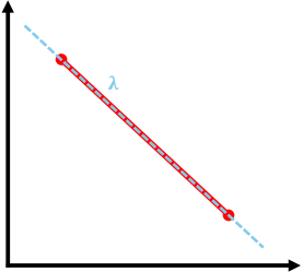
(a) Linear

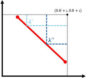
(b) Tchebycheff

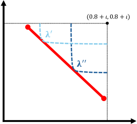
(c) Smooth Tchebycheff

Figure 1: Example of Scalarization Methods for Stochastic Policy Class. Consider a bi-objective multi-arm bandit problem with stochastic policies, whose reward functions are $r_{1}(a_{1})=0.2,r_{1}(a_{2})=0.8$ and $r_{2}(a_{1})=0.8,r_{2}(a_{2})=0.2$. The red dots in the figures are $(r_{1}(a_{1}),r_{2}(a_{1}))$ and $(r_{1}(a_{2}),r_{2}(a_{2}))$. The red lines represent reward values under all stochastic Pareto optimal policies. We show the level sets of different scalarization functions in terms of $(r_{1},r_{2})$, i.e., Linear scalarization $\sum_{i=1}^{2}\lambda_{i}r_{i}$, Tchebycheff scalarization $\max_{i}\lambda_{i}(0.8+\iota-r_{i})$, and smooth Tchebycheff scalarization $\mu\log\sum_{i=1}^{2}e^{\frac{\lambda_{i}(0.8+\iota-r_{i})}{\mu}}$. The blue dotted lines are the level sets for the optimal (maximal or minimal) scalarization function values with $(r_{1},r_{2})$ defined on the red lines. Then, linear scalarization does not differentiate different Pareto values, but (smooth) Tchebycheff scalarization can identify each point by setting different $\bm{\lambda}$, showing better solution controllability.

Remark 4.9 (Linear Scalarization vs. Tchebycheff Scalarization.).

From the above propositions, we can observe that for the deterministic policy class, Tchebycheff scalarization can find all Pareto optimal policies, whereas linear scalarization fails to do so. Additionally, for the stochastic policy class, we discover that it is computationally difficult to identify all representative Pareto optimal policies utilizing linear scalarization under certain situations. Particularly, when $\bm{V}_{1}^{\pi}(s_{1})$ for a set of Pareto optimal policies $\pi$ lie on a hyperplane in the form of $\overline{\bm{\lambda}}^{\top}\bm{V}_{1}^{\pi}(s_{1})=C$ for some $C>0$ and $\overline{\bm{\lambda}}$, then we need to find all the solutions to $\max_{\pi}\mathrm{LIN}_{\overline{\bm{\lambda}}}(\pi)$, since all these Pareto optimal policies have the same preference $\overline{\bm{\lambda}}$ defined based on linear scalarization. In contrast, Proposition 4.8 indicates that for each of $\bm{V}_{1}^{\pi}(s_{1})$ on $\overline{\bm{\lambda}}^{\top}\bm{V}_{1}^{\pi}(s_{1})=C$ under different $\pi$’s, we can use different $\bm{\lambda}$’s that are associated with distinct $\pi$’s and solve $\min_{\pi}\mathrm{TCH}_{\bm{\lambda}}(\pi)$ to obtain one representative policy for each $\bm{\lambda}$. In Figure 1, we illustrate the above discussion via a bi-objective multi-arm bandit example. The discussion above implies that Tchebycheff scalarization has better controllability over its solution and thus is recognized as a favorable scalarization method for MORL. Furthermore, in Section 7, we study an extension of Tchebycheff scalarization named smooth Tchebycheff scalarization, which also has a better controllability of its solution compared to the linear scalarization. We refer readers to Section 7 for more details, where we prove that the smooth Tchebycheff scalarization offers a more advantageous property compared to the original Tchebycheff scalarization in finding Pareto optimal policies. In Table 1, we provide a detailed comparison of different scalarization methods.

5 MORL via Tchebycheff Scalarization

In this section, we propose an efficient algorithm to solve $\min_{\pi\in\Pi}\mathrm{TCH}_{\bm{\lambda}}(\pi)$ for any given $\bm{\lambda}$. We note that since all our proposed algorithms in this paper allow mixture policies and utilize the minimax theorem (v. Neumann, 1928), according to Wu et al. (2021b); Miryoosefi and Jin (2022), the proposed algorithms only solve the problem within a stochastic policy class $\Pi$. However, for the deterministic policy class, one may need different algorithmic design ideas to solve this problem. We leave designing efficient algorithms for the deterministic policy class as an open question.

Reformulation of Tchebycheff Scalarization. We note that although (4) has favorable properties, it is a non-smooth function, and thus $\min_{\pi\in\Pi}\mathrm{TCH}_{\bm{\lambda}}(\pi)$ is difficult to solve directly. To resolve this challenge, we propose the following equivalent form for Tchebycheff scalarization loss.

Proposition 5.1 (Equivalent form of TCH).

Letting $\bm{w}=(w_{1},w_{2},\cdots,w_{m})\in\Delta_{m}$, the Tchebycheff scalarization is reformulated as $\mathrm{TCH}_{\bm{\lambda}}(\pi)=\max_{\bm{w}\in\Delta_{m}}\max_{\{\nu_{i}\in\Pi\}_{i=1}^{m}}\sum_{i=1}^{m}w_{i}\lambda_{i}(V_{i,1}^{\nu_{i}}(s_{1})+\iota-V_{i,1}^{\pi}(s_{1}))$. Then, the minimization problem of Tchebycheff scalarization is reformulated as

$$\min_{\pi\in\Pi}\mathrm{TCH}_{\bm{\lambda}}(\pi)=\min_{\pi\in\Pi}\max_{\bm{w}\in\Delta_{m}}\max_{\{\nu_{i}\in\Pi\}_{i=1}^{m}}\sum_{i=1}^{m}w_{i}\lambda_{i}\big{(}V_{i,1}^{\nu_{i}}(s_{1})+\iota-V_{i,1}^{\pi}(s_{1})\big{)}.$$ (5)

Proposition 5.1 converts the original problem into a min-max-max problem, which can avoid a non-smooth objective function and thus is expected to have a nice convergence performance. This formulation can better fit the UBC-based algorithmic framework, which motivates us to design efficient optimistic MORL algorithms. Furthermore, we remark that the above proposition also offers a feasible reformulation of Tchebycheff scalarization that can be better applied to multi-objective stochastic optimization or multi-objective online learning, which are not restricted to MORL.

Algorithm. We now propose an algorithm named TchRL to solve (5), as summarized in Algorithm 1, that can efficiently learn the (weakly) Pareto optimal solution for a given preference vector $\bm{\lambda}$. According to (5), to solve such a min-max-max optimization problem, Algorithm 1 features three alternate updating procedures to update $\bm{w}^{t}$, auxiliary policies $\nu_{i}^{t}$ for $i\in[m]$, and the main policy $\pi^{t}$, along with optimistic estimation of Q-functions to facilitate exploration.

Specifically, as (5) aims to maximize $\bm{w}$, Line 3 performs a mirror ascent step, which can keep any of its iterates in $\Delta_{m}$ without an extra projection step. The update of $\bm{w}^{t}$ is equivalent to solving a maximization problem as

$$\max_{\bm{w}\in\Delta_{m}}\eta\langle\bm{w},\bm{\lambda}\odot(\widetilde{\bm{V}}_{1}^{t-1}(s_{1})+\bm{\iota}-\bm{V}_{1}^{t-1}(s_{1}))\rangle-D_{\mathrm{KL}}(\bm{w},\bm{w}^{t-1}),$$

where $D_{\mathrm{KL}}(\bm{x},\bm{y}):=\sum_{i=1}^{m}x_{i}\log(x_{i}/y_{i})$ is the Kullback–Leibler (KL) divergence, $\bm{\iota}$ is an all-$\iota$ vector, and $\widetilde{\bm{V}}_{1}^{t-1}:=(\widetilde{V}_{1,1}^{t-1},\cdots,\widetilde{V}_{m,1}^{t-1})$, and $\bm{V}_{1}^{t-1}:=(V_{1,1}^{t-1},\cdots,V_{m,1}^{t-1})$ from the last round. In addition, Algorithm 1 updates two types of policies, i.e., the auxiliary policies $\widetilde{\nu}_{i}^{t},\forall i\in[m],$ and the main policy $\pi^{t}$, respectively in Line 6 and Line 8. The auxiliary policy $\widetilde{\nu}_{i}^{t}$ tracks the individual optimal policy $\nu_{i}^{*}:=\mathop{\mathrm{argmax}}_{\nu_{i}}V_{i,1}^{\nu_{i}}(s_{1})$ for the $i$-th objective associated with the reward function $r_{i}$, while $\pi^{t}$ is the estimate of $\pi_{\bm{\lambda}}^{*}:=\min_{\pi\in\Pi}\mathrm{TCH}_{\bm{\lambda}}(\pi)$, namely, the (weakly) Pareto optimal policy under the given preference $\bm{\lambda}$. We further employ two Q-functions, $\widetilde{Q}_{i,h}^{t}$ and $Q_{i,h}^{t}$, as estimates of $Q_{i,h}^{\nu_{i}^{*}}$ and $Q_{i,h}^{\pi_{\bm{\lambda}}^{*}}$. Thus, $\widetilde{\nu}_{i}^{t}$ is obtained solely based on $\widetilde{Q}_{i,h}^{t}$, while $\pi^{t}$ is updated by a linear combination of $\widetilde{Q}_{i,h}^{t}$ over all $i\in[m]$ by $\bm{w}^{t}\odot\bm{\lambda}$, incorporating the preference $\bm{\lambda}$ and the current weight $\bm{w}^{t}$. Due to the greedy updating rules for both policies, $\widetilde{\nu}_{i,h}^{t}$ and $\pi_{h}^{t}$ are hence deterministic policies based on $\widetilde{Q}_{i,h+1}^{t}$ and $(\bm{w}^{t}\odot\bm{\lambda})^{\top}Q_{h}^{t}$. Here, the Q-functions $\widetilde{Q}_{i,h}^{t}$ and $Q_{i,h}^{t}$ are constructed via “the principle of optimism in the face of uncertainty” by calling Subroutine 1, which will be elaborated below. In Lines 9 and 10, we further sample trajectories following $\widetilde{\nu}_{i}^{t}$ and $\pi_{i}^{t}$ to update the datasets $\widetilde{\mathcal{D}}_{i,h}$ and $\mathcal{D}_{i,h}$ respectively for the construction of $\widetilde{Q}_{i,h}^{t+1}$ and $Q_{i,h}^{t+1}$ in the next round.

The function OptQ in Subroutine 1 performs optimistic Q-function construction based on the collected trajectories $\{s_{h}^{\tau},a_{h}^{\tau},s_{h+1}^{\tau},r_{i,h}^{\tau}(s_{h}^{\tau},a_{h}^{\tau})\}_{h,\tau=1}^{H,\ell-1}$, and returns the optimistic Q-function $Q_{i,h}$. It first estimates the reward functions $\widehat{r}_{i}^{\ell}$ and transition model $\widehat{\mathbb{P}}^{\ell}$ as well as bonus terms $\Psi_{i,h}^{\ell}$ and $\Phi_{h}^{\ell}$ for such a construction. The bonus terms will then have larger values for less-explored state-action pairs and thus facilitate the exploration of those state-action pairs during the learning process. Our work considers a tabular case such that the reward functions and transition are estimated by

$$\widehat{r}_{i,h}^{\ell}(s,a)=\frac{\sum_{\tau=1}^{\ell-1}\mathbf{1}_{\{(s,a)=(s_{h}^{\tau},a_{h}^{\tau})\}}r_{i,h}^{\tau}}{N_{h}^{\ell-1}(s,a)\vee 1},\quad\widehat{\mathbb{P}}_{h}^{\ell}(s^{\prime}|s,a)=\frac{N_{h}^{\ell-1}(s,a,s^{\prime})}{N_{h}^{\ell-1}(s,a)\vee 1},$$ (6)

where $\mathbf{1}_{\{\cdot\}}$ is an indicator function, $N_{h}^{\ell-1}(s,a,s^{\prime})=\sum_{\tau=1}^{\ell-1}\mathbf{1}_{\{(s,a,s^{\prime})=(s_{h}^{\tau},a_{h}^{\tau},s_{h+1}^{\tau})\}}$ and $N_{h}^{\ell-1}(s,a)=\sum_{\tau=1}^{\ell-1}\mathbf{1}_{\{(s,a)=(s_{h}^{\tau},a_{h}^{\tau})\}}$. Denoting $x\vee y=\max\{x,y\}$ and $x\wedge y=\min\{x,y\}$, the reward bonus and transition bonus terms are constructed by

$$\Psi_{i,h}^{\ell}(s,a)=\sqrt{\frac{2\log(8m|{\mathcal{S}}||\mathcal{A}|HT/\delta)}{N_{h}^{\ell-1}(s,a)\vee 1}}\wedge 1,\quad\Phi_{h}^{\ell}(s,a)=\sqrt{\frac{2H^{2}|{\mathcal{S}}|\log(8m|{\mathcal{S}}||\mathcal{A}|HT/\delta)}{N_{h}^{\ell-1}(s,a)\vee 1}}\wedge H,$$ (7)

such that the true reward and transition satisfy $|\widehat{r}_{i,h}^{\ell-1}(s,a)-r_{i,h}(s,a)|\leq\Psi_{i,h}^{\ell}(s,a)$ and $|\widehat{\mathbb{P}}_{h}^{\ell}V(s,a)-\mathbb{P}_{h}V(s,a)|\leq\Phi_{h}^{\ell}(s,a)$ for any function $V:{\mathcal{S}}\mapsto[0,H]$ with probability at least $1-\delta$. This relation can be verified by applying Hoeffding’s inequality, as shown in our appendix.

Algorithm 1 TchRL: Multi-Objective RL via Tchebycheff Scalarization

1:Initialize: $\bm{\lambda}$, $\pi_{h}^{0}(\cdot|\cdot)=\nu_{i,h}^{0}(\cdot|\cdot)=\mathrm{Unif}(\mathcal{A})$, $\mathcal{D}_{i}=\widehat{\mathcal{D}}_{i}=\varnothing$, $w_{i}^{0}=1/m$, $V_{i,h}^{0}(\cdot)=\widetilde{V}_{i,h}^{0}(\cdot)=0,\forall(i,h)$

2:for $t=1,2,\ldots,T$ do

3:    Update $\bm{w}$ via $w_{i}^{t}\propto w_{i}^{t-1}\cdot\exp\{\eta\cdot\lambda_{i}(\widetilde{V}_{i,1}^{t-1}(s_{1})+\iota-V_{i,1}^{t-1}(s_{1}))\},~{}\forall i\in[m]$

4:    for $h=H,H-1,\ldots,1$ do

5:         $\widetilde{Q}_{i,h}^{t}=\texttt{OptQ}\big{(}\widetilde{\mathcal{D}}_{i,h},\widetilde{V}_{i,h+1}^{t}\big{)}$ where $\widetilde{V}_{i,h+1}^{t}(\cdot)=\langle\widetilde{Q}_{i,h+1}^{t}(\cdot,\cdot),\widetilde{\nu}_{i,h+1}^{t}(\cdot|\cdot)\rangle_{\mathcal{A}},~{}\forall i\in[m]$

6:         Update auxiliary policies $\widetilde{\nu}_{i,h}^{t}=\mathop{\mathrm{argmax}}_{\nu_{h}}\langle\widetilde{Q}_{i,h}^{t}(\cdot,\cdot),\nu_{h}(\cdot|\cdot)\rangle_{\mathcal{A}},~{}\forall i\in[m]$

7:         $Q_{i,h}^{t}=\texttt{OptQ}\big{(}\mathcal{D}_{i,h},V_{i,h+1}^{t}\big{)}$ where $V_{i,h+1}^{t}(\cdot)=\langle Q_{i,h+1}^{t}(\cdot,\cdot),\pi_{h+1}^{t}(\cdot|\cdot)\rangle_{\mathcal{A}},\forall i\in[m]$

8:         Update main policy $\pi_{h}^{t}=\mathop{\mathrm{argmax}}_{\pi_{h}}\langle(\bm{w}^{t}\odot\bm{\lambda})^{\top}\bm{Q}_{h}^{t}(\cdot,\cdot),\pi_{h}(\cdot|\cdot)\rangle_{\mathcal{A}}$     

9:    Sample data $\{\widetilde{s}_{i,h}^{t},\widetilde{a}_{i,h}^{t},\widetilde{s}_{i,h+1}^{t},\widetilde{r}_{i,h}^{t}\}_{h=1}^{H}\sim(\widetilde{\nu}_{i}^{t},\mathbb{P})$ and append it to $\widetilde{\mathcal{D}}_{i,h},~{}\forall(i,h)$

10:    Sample data $\{s_{h}^{t},a_{h}^{t},s_{h+1}^{t},(r_{i,h}^{t})_{i=1}^{m}\}_{h=1}^{H}\sim(\pi^{t},\mathbb{P})$ and append $(s_{h}^{t},a_{h}^{t},s_{h+1}^{t},r_{i,h}^{t})$ to $\mathcal{D}_{i,h},~{}\forall(i,h)$

11:Return: $\{\pi^{t}\}_{t=1}^{T}$

Subroutine 1 OptQ: Optimistic Q-Function Construction

1: Function: OptQ$\big{(}\{s_{h}^{\tau},a_{h}^{\tau},s_{h+1}^{\tau},r_{i,h}^{\tau}(s_{h}^{\tau},a_{h}^{\tau})\}_{h,\tau=1}^{H,\ell-1},V_{i,h+1}\big{)}$ $\triangleright$ Construct optimistic Q-function

2:Calculate reward and transition estimates $\widehat{r}_{h}^{\ell}$, $\widehat{\mathbb{P}}_{h}^{\ell}$ via (6)

3:Calculate reward and transition bonuses $\Psi_{i,h}^{\ell}$, $\Phi_{h}^{\ell}$ via (7)

4:$Q_{i,h}(\cdot,\cdot)=\{(\widehat{r}_{i,h}^{\ell}+\widehat{\mathbb{P}}_{h}^{\ell}V_{i,h+1}+\Phi_{h}^{\ell}+\Psi_{i,h}^{\ell})(\cdot,\cdot)\}_{[0,H-h+1]}$

5:Return: $\{Q_{i,h}\}_{h=1}^{H}$

Theoretical Result. The following theorem provides a theoretical guarantee for Algorithm 1.

Theorem 5.2 (Theoretical Guarantee for TchRL).

Setting $\eta=\sqrt{\log m/(H^{2}T)}$, letting $\widehat{\pi}:=\mathrm{Mix}(\pi^{1},\pi^{2},\cdots,\pi^{T})$ be a mixture of the learned policies, $\pi_{\bm{\lambda}}^{*}\in\mathop{\mathrm{argmin}}_{\pi\in\Pi}\mathrm{TCH}_{\bm{\lambda}}(\pi)$ for any preference vector $\bm{\lambda}\in\Delta_{m}$, then with probability at least $1-\delta$, after $T$ rounds of Algorithm 1, we obtain

$$\mathrm{TCH}_{\bm{\lambda}}(\widehat{\pi})-\mathrm{TCH}_{\bm{\lambda}}(\pi_{\bm{\lambda}}^{*})\leq\mathcal{O}\Big{(}\sqrt{H^{4}|{\mathcal{S}}|^{2}|\mathcal{A}|\varrho/T}\Big{)},$$

where $\varrho:=\log(m|{\mathcal{S}}||\mathcal{A}|HT/\delta)$.

When we set $T=\widetilde{\mathcal{O}}(H^{4}|{\mathcal{S}}|^{2}|\mathcal{A}|/\varepsilon^{2})$, we are able to achieve $\mathrm{TCH}_{\bm{\lambda}}(\widehat{\pi})-\mathrm{TCH}_{\bm{\lambda}}(\pi_{\bm{\lambda}}^{*})\leq\varepsilon$, where $\widetilde{\mathcal{O}}$ hides logarithmic dependence on $\varepsilon^{-1}$, $H$, $|{\mathcal{S}}|$, $|\mathcal{A}|$, and $m$. It implies that for one $\bm{\lambda}$, Algorithm 1 requires $\widetilde{\mathcal{O}}(mH^{4}|{\mathcal{S}}|^{2}|\mathcal{A}|/\varepsilon^{2})$ sample complexity to achieve an $\varepsilon$-error, where the extra factor $m$ is from the $m$ rounds of exploration in Lines 9 and 10.

Denoting $\widehat{\pi}$ as a mixture of $\{\pi^{1},\pi^{2},\cdots,\pi^{T}\}$, we let $\widehat{\pi}$ be the output of this algorithm, following prior RL works Miryoosefi and Jin (2022); Wu et al. (2021b); Altman (2021). The policy $\widehat{\pi}$ is executed by randomly selecting a policy $\pi^{t}$ from $\{\pi^{1},\pi^{2},\cdots,\pi^{T}\}$ with equal probability beforehand and then exclusively following $\pi^{t}$ thereafter, which implies $V^{\widehat{\pi}}_{i,1}(s_{1})=\frac{1}{T}\sum_{t=1}^{T}V^{\pi^{t}}_{i,1}(s_{1})$ (Wu et al., 2021b; Miryoosefi and Jin, 2022) for theoretical analysis.

Moreover, we can also use the notion of the occupancy measure to estimate $\widehat{\pi}$. Specifically, denoting by $\theta_{h}(s,a;\pi)$ the joint distribution of $(s,a)$ at step $h$ induced by $\pi$ and $\mathbb{P}$, we have $V^{\pi}_{i,1}(s_{1})=\sum_{h=1}^{H}\sum_{s\in{\mathcal{S}}}\sum_{a\in\mathcal{A}}\theta_{h}(s,a;\pi)r_{i,h}(s,a)$. The occupancy measure can be dynamically calculated as $\theta_{h+1}(s^{\prime},a^{\prime};\pi)=\sum_{s\in{\mathcal{S}}}\sum_{a\in\mathcal{A}}\theta_{h}(s,a;\pi)\mathbb{P}_{h}(s^{\prime}|s,a)\pi_{h+1}(a^{\prime}|s^{\prime})$. The policy $\pi$ can be recovered as $\pi_{h}(a|s)=\frac{\theta_{h}(s,a;\pi)}{\sum_{a\in\mathcal{A}}\theta_{h}(s,a;\pi)}$. By the definition of the policy mixture, we have $\theta_{h}(s,a;\widehat{\pi})=\frac{1}{T}\sum_{t=1}^{T}\theta_{h}(s,a;\pi^{t})$. If we know the true transition $\mathbb{P}$, we can recover $\widehat{\pi}$ by $\theta_{h}(s,a;\widehat{\pi})$. Practically, we can substitute $\mathbb{P}$ with an estimate of $\widehat{\mathbb{P}}^{T-1}$. When $T$ is large enough, the estimate of $\widehat{\pi}$ will be sufficiently accurate. For the multi-arm bandit problem, since it has no transition model, we directly have $\widehat{\pi}=\frac{1}{T}\sum_{t=1}^{T}\pi^{t}$.

To avoid the policy mixture, a more intriguing future direction is to further explore the theoretical guarantee of the last-iterate convergence along with using variants of policy optimization methods, which demands a more complex algorithmic design.

Remark 5.3.

Algorithm 1 constructs optimistic Q-functions based on trajectories generated by their own corresponding policies $\pi^{t}$ and $\widetilde{\nu}_{i}^{t},\forall i\in[m],$ as in Lines 9 and 10. It is intriguing to investigate off-policy algorithmic designs (Andrychowicz et al., 2017; Yu et al., 2021a), such as hindsight experience replay and importance sampling, to improve sample efficiency by utilizing data across policies. Such a topic is of independent interest and the related theoretical analysis can be left as a future research direction. However, in the next section, our new algorithm can avoid such multiple exploration rounds by an uncertainty-guided preference-free exploration method.

Remark 5.4.

Tchebycheff scalarization does not explicitly distinguish between Pareto optimal policies and other weakly Pareto optimal policies based on the setting of $\bm{\lambda}$. One may consider using $\frac{1}{T}\sum_{t=1}^{T}V^{t}_{i,1}(s_{1})$ to estimate $V^{\widehat{\pi}}_{i,1}(s_{1})=\frac{1}{T}\sum_{t=1}^{T}V^{\pi^{t}}_{i,1}(s_{1})$ for a sufficiently large $T$ and comparing the estimated values of $V^{\widehat{\pi}}_{i,1}(s_{1})$ under different $\bm{\lambda}$ to rule out non-Pareto-optimal policies within certain error tolerance, which, however, might be numerically unstable. In practice, weakly Pareto optimal policies are often considered acceptable solutions as they can also capture the trade-off of learners’ preferences across different objectives, especially when $\mathbb{V}(\Pi)$ is convex for a stochastic policy $\Pi$.

6 Preference-Free MORL via Tchebycheff Scalarization

Algorithm. Although Algorithm 1 has the controllability of the policy learning that can incorporate learner’s preference $\bm{\lambda}$, it always requires exploration of the environment once a new preference vector $\bm{\lambda}$ is given, which will incur high costs of environment interaction if many different preferences are considered. This motivates us to further design a new preference-free algorithmic framework named PF-TchRL. This new algorithm features decoupled exploration and planning phases as summarized in Algorithms 2 and 3. Once the exploration stage, i.e., Algorithm 2, thoroughly explores the environment to collect trajectories $\mathcal{D}$ without any designated preference $\bm{\lambda}$, we can then execute the planning phase, Algorithm 3, using $\mathcal{D}$ for any diverse input preferences $\bm{\lambda}\in\Delta_{m}$, requiring no additional environment interaction.

Specifically, in Algorithm 2, Line 4 estimates the transition model and bonus terms, where $\widehat{\mathbb{P}}_{h}^{t}$, $\Psi_{i,h}^{t}$, and $\Phi_{h}^{t}$ are instantiated according to (6) and (7) with collected trajectories before the $t$-th exploration round, i.e., $\{s_{h}^{\tau},a_{h}^{\tau},s_{h+1}^{\tau}\}_{h,\tau=1}^{H,t-1}$. Furthermore, in Line 5, we define the exploration reward $\overline{r}_{h}^{t}$ based on the reward and transition bonus terms. Such a reward design can guide the agent to explore the most uncertain state-action pairs, where the uncertainty is characterized by both reward and transition bonus terms. There are two construction options for the exploration reward: option [I] employs a maximum operation on bonuses, and option [II] takes summation over all bonuses, leading to different theoretical results presented below. Then, Line 6 constructs an optimistic Q-function $\overline{Q}_{h}^{t}$ based on the estimated transition, the transition bonus that guarantees optimism, and the exploration reward. Line 7 generates the exploration policy $\overline{\pi}^{t}$, via which we further sample data as in Line 8. Note that although we collect rewards in Line 8, they are not used to construct $\overline{Q}_{h}^{t}$ as the exploration is only guided by uncertainty-based explore reward $\overline{r}^{t}$ rather than the estimated true reward, such that the collected data can have a sufficiently wide coverage of all policies.

Finally, in the planning phase, i.e., Algorithm 3, we first estimate the reward and transition as

$$\begin{aligned} \widehat{r}_{i,h}(s,a)=\frac{\sum_{\tau=1}^{T}\mathbf{1}_{\{(s,a)=(s_{h}^{\tau},a_{h}^{\tau})\}}r_{i,h}^{\tau}}{N_{h}^{T}(s,a)\vee 1},\quad\widehat{\mathbb{P}}_{h}(s^{\prime}|s,a)=\frac{N_{h}^{T}(s,a,s^{\prime})}{N_{h}^{T}(s,a)\vee 1},\end{aligned}$$ (8)

and calculate their bonus terms as

$$\begin{aligned} \Psi_{i,h}(s,a)=\sqrt{\frac{2\log(8m|{\mathcal{S}}||\mathcal{A}|HT/\delta)}{N_{h}^{T}(s,a)\vee 1}}\wedge 1,\quad\Phi_{h}(s,a)=\sqrt{\frac{2H^{2}|{\mathcal{S}}|\log(8m|{\mathcal{S}}||\mathcal{A}|HT/\delta)}{N_{h}^{T}(s,a)\vee 1}}\wedge H,\end{aligned}$$ (9)

based on the pre-collected data $\mathcal{D}$ in Algorithm 2. Then, for any input preference $\bm{\lambda}$, we construct optimistic Q-functions, calculate $\widetilde{\nu}_{i}$ to estimate $\widetilde{\nu}_{i}^{*}$, and iteratively update $\bm{w}^{k}$ and $\pi^{k}$ for $K$ rounds without further exploration, which significantly saves the exploration cost. The updating steps of $\bm{w}^{k}$ and $\pi^{k}$ share a similar spirit as the ones in Algorithm 1. The updating rule of $\bm{w}^{k}$ is a mirror ascent step, equivalent to solving the following problem.

$$\max_{\bm{w}\in\Delta_{m}}\eta_{k-1}\langle\bm{w},\bm{\lambda}\odot(\widetilde{\bm{V}}_{1}^{k-1}(s_{1})+\bm{\iota}-\bm{V}_{1}^{k-1}(s_{1}))\rangle-D_{\mathrm{KL}}(\bm{w},\bm{w}^{k-1}).$$

Algorithm 2 Preference-Free Exploration Stage for Multi-Objective RL

1:Initialize: $\overline{\pi}_{h}^{0}(\cdot|\cdot)=\mathrm{Unif}(\mathcal{A}),\forall h\in[H]$, $\mathcal{D}=\varnothing$

2:for $t=1,\ldots,T$ do

3:    for $h=H,H-1,\ldots,1$ do

4:         Calculate the transition estimate $\widehat{\mathbb{P}}_{h}^{t}$, and reward and transition bonuses $\Psi_{i,h}^{t}$, $\Phi_{h}^{t}$, $\forall(i,h)$

5:         Uncertainty-guided exploration reward $\overline{r}_{h}^{t}(\cdot,\cdot)=\begin{cases}\max\{\Phi_{h}^{t}(\cdot,\cdot)/H,\Psi_{1,h}^{t}(\cdot,\cdot),\cdots,\Psi_{m,h}^{t}(\cdot,\cdot)\}~{}~{}\text{[{I}]}\\ \Phi_{h}^{t}(\cdot,\cdot)/H+\sum_{i=1}^{m}\Psi_{i,h}^{t}(\cdot,\cdot)\qquad\qquad\qquad~{}\text{[{II}]}\end{cases}$

6:         $\overline{Q}_{h}^{t}(\cdot,\cdot)=\{(\overline{r}_{h}^{t}+\widehat{\mathbb{P}}_{h}^{t}\overline{V}_{h+1}^{t}+\Phi_{h}^{t})(\cdot,\cdot)\}_{[0,H-h+1]}$ where $\overline{V}_{h+1}^{t}(\cdot)=\langle\overline{Q}_{h+1}^{t}(\cdot,\cdot),\overline{\pi}_{h+1}^{t}(\cdot|\cdot)\rangle_{\mathcal{A}}$

7:         Generate exploration policy $\overline{\pi}_{h}^{t}=\mathop{\mathrm{argmax}}_{\pi_{h}}\big{\langle}\overline{Q}_{h}^{t}(\cdot,\cdot),\pi_{h}(\cdot|\cdot)\big{\rangle}_{\mathcal{A}}$     

8:    Uncertainty-guided sampling $\{s_{h}^{t},a_{h}^{t},s_{h+1}^{t},(r_{i,h}^{t})_{i=1}^{m}\}_{h=1}^{H}\sim(\overline{\pi}^{t},\mathbb{P})$ and append it to $\mathcal{D}$

9:Return: $\mathcal{D}$

Algorithm 3 Planning Stage for PF-TchRL

1:Input: Preference $\bm{\lambda}$ and pre-collected data $\mathcal{D}:=\{s_{h}^{t},a_{h}^{t},s_{h+1}^{t},(r_{i,h}^{t})_{i=1}^{m}\}_{t=1}^{T}$ by Algorithm 2

2:Initialize: $\eta_{0}=0$, $V_{i,h}^{0}(\cdot)=0$, $w_{i}^{0}=1/m$, $\widetilde{V}_{i,H+1}(\cdot)=0,~{}\forall(i,h)\in[m]\times[H]$

3:Calculate reward and transition estimates $\widehat{r}_{i,h}$, $\widehat{\mathbb{P}}_{h}$ and bonus terms $\Psi_{i,h}$, $\Phi_{h}$ via (8) (9), $\forall(i,h)$

4:for $h=H,H-1,\ldots,1$ do

5:    $\widetilde{Q}_{i,h}(\cdot,\cdot)=\{(\widehat{r}_{i,h}+\widehat{\mathbb{P}}_{h}\widetilde{V}_{i,h+1}+\Phi_{h}+\Psi_{i,h})(\cdot,\cdot)\}_{[0,H-h+1]},~{}\forall i\in[m]$

6:    $\widetilde{\nu}_{i,h}=\mathop{\mathrm{argmax}}_{\nu_{h}}\langle\widetilde{Q}_{i,h}(\cdot,\cdot),\nu_{h}(\cdot|\cdot)\rangle_{\mathcal{A}}$ and let $\widetilde{V}_{i,h}(\cdot)=\langle\widetilde{Q}_{i,h}(\cdot,\cdot),\widetilde{\nu}_{i,h}(\cdot|\cdot)\rangle_{\mathcal{A}},\forall i\in[m]$

7:for $k=1,\ldots,K$ do

8:    Update $\bm{w}$ via $w_{i}^{k}\propto w_{i}^{k-1}\cdot\exp\{\eta_{k-1}\cdot\lambda_{i}(\widetilde{V}_{i,1}(s_{1})+\iota-V_{i,1}^{k-1}(s_{1}))\},~{}\forall i\in[m]$

9:    for $h=H,H-1,\ldots,1$ do

10:         $Q_{i,h}^{k}(\cdot,\cdot)=\{(\widehat{r}_{i,h}+\widehat{\mathbb{P}}_{h}V_{i,h+1}^{k}+\Phi_{h}+\Psi_{i,h})(\cdot,\cdot)\}_{[0,H-h+1]},~{}\forall i\in[m]$

11:         $\pi_{h}^{k}=\mathop{\mathrm{argmax}}_{\pi_{h}}\langle(\bm{w}^{k}\odot\bm{\lambda})^{\top}\bm{Q}_{h}^{k}(\cdot,\cdot),\pi_{h}(\cdot|\cdot)\rangle_{\mathcal{A}}$ and let $V_{i,h}^{k}(\cdot)=\langle Q_{i,h}^{k}(\cdot,\cdot),\pi_{h}^{k}(\cdot|\cdot)\rangle_{\mathcal{A}},\forall i\in[m]$     

12:Return: $\{\pi^{k}\}_{k=1}^{K}$

Remark 6.1 (Exploration Reward).

Line 5 in Algorithm 2 defines the exploration reward $\overline{r}^{t}$ by taking maximum over bonus terms in option [I]. We note that option [I] fits the case where bonus terms share the same structure, e.g., $1/\sqrt{N_{h}^{t-1}(s,a)\vee 1}$ in the tabular case. Thus, the maximum is indeed taken over the factors other than $1/\sqrt{N_{h}^{t-1}(s,a)\vee 1}$ in bonus terms. For general cases, when there is no such similar structure, e.g., different feature representations in function approximation settings, we can apply a summation of all bonuses as in option [II], which, however, will introduce extra an $\mathcal{O}(m)$ term to the exploration complexity as we show in our theoretical result. It remains an intriguing direction to study our proposed algorithms under various function approximation settings.

Remark 6.2 (Comparison with Reward-Free RL).

Algorithm 2 shares a similar spirit to the prior reward-free exploration methods (e.g., Wang et al. (2020); Qiu et al. (2021b); Jin et al. (2020a); Zhang et al. (2023, 2021)) but has two differences: (1) Algorithm 2 defines exploration rewards $\overline{r}^{t}$ using both reward and transition uncertainties, and (2) it also collects rewards for reward estimation in the planning phase. Reward-free RL defines $\overline{r}^{t}$ solely based on the transition bonus, and the reward function is fully given instead of being estimated. Hence, Algorithm 2 generalizes these prior reward-free exploration methods. The MORL work (Wu et al., 2021a) also proposes a preference-free algorithm. But its algorithm is very similar to the prior reward-free methods as the reward function is not estimated and is directly given in the planning phase. We remark that Algorithm 2 is not limited to the Tchebycheff scalarization, but can be applied to any MORL scalarization technique. As shown in the following section, Algorithm 2 is also utilized for the smooth Tchebycheff scalarization.

Theoretical Result. The following theorem provides theoretical guarantee for Algorithms 2 and 3.

Theorem 6.3 (Theoretical Guarantee for PF-TchRL).

Setting $\eta_{k}=\sqrt{\log m/(H^{2}K)}$ if $k>0$ and $0$ otherwise, letting $\widehat{\pi}:=\mathrm{Mix}(\pi^{1},\pi^{2},\cdots,\pi^{K})$ be a mixture of the learned policies and $\pi_{\bm{\lambda}}^{*}\in\mathop{\mathrm{argmin}}_{\pi\in\Pi}\mathrm{TCH}_{\bm{\lambda}}(\pi)$ for any preference vector $\bm{\lambda}\in\Delta_{m}$, then with probability at least $1-\delta$, after $T$ rounds of exploration via Algorithm 2 and $K$ rounds of planning via Algorithm 3, we obtain

$$\mathrm{[\mathbf{I}]:} \quad\mathrm{TCH}_{\bm{\lambda}}(\widehat{\pi})-\mathrm{TCH}_{\bm{\lambda}}(\pi_{\bm{\lambda}}^{*})\leq\mathcal{O}\Big{(}\sqrt{H^{2}\log m/K}+\sqrt{H^{6}|{\mathcal{S}}|^{2}|\mathcal{A}|\varrho/T}\Big{)},$$

$$\mathrm{[\mathbf{II}]:} \quad\mathrm{TCH}_{\bm{\lambda}}(\widehat{\pi})-\mathrm{TCH}_{\bm{\lambda}}(\pi_{\bm{\lambda}}^{*})\leq\mathcal{O}\Big{(}\sqrt{H^{2}\log m/K}+\sqrt{(H^{2}|{\mathcal{S}}|+m)H^{4}|{\mathcal{S}}||\mathcal{A}|\varrho/T}\Big{)}.$$

where $\varrho:=\log(m|{\mathcal{S}}||\mathcal{A}|HT/\delta)$, and [I] and [II] correspond to different options in Algorithm 2.

Setting the numbers of the planning steps $K=\widetilde{\mathcal{O}}(H^{2}/\varepsilon^{2})$ and the exploration rounds $T=\widetilde{\mathcal{O}}(H^{6}|{\mathcal{S}}|^{2}|\mathcal{A}|/\varepsilon^{2})$ for option [I] or $T=\widetilde{\mathcal{O}}((H^{2}|{\mathcal{S}}|+m)H^{4}|{\mathcal{S}}||\mathcal{A}|/\varepsilon^{2})$ for option [II], we can achieve $\mathrm{TCH}_{\bm{\lambda}}(\widehat{\pi})-\mathrm{TCH}_{\bm{\lambda}}(\pi_{\bm{\lambda}}^{*})\leq\varepsilon$. We can see option [II] has an extra dependence on $m$, stemming from the sum operation of all bonus terms. Moreover, compared with Theorem 5.2, Theorem 6.3 has an additional factor $H^{2}$ which is also observed in the prior reward-free RL works when compared with online algorithms (see, e.g., Jin et al. (2020b); Wang et al. (2020); Yang et al. (2020); Qiu et al. (2021b)). However, although such an extra factor $H^{2}$ exists, when a learner expects to have sufficient coverage of the (weakly) Pareto optimal set under a large number of preferences $\bm{\lambda}\in\Delta_{m}$, Algorithm 1 requires exploration for every $\bm{\lambda}$, while Algorithm 2 only explore once, significantly saving the exploration cost.

7 Extension to Smooth Tchebycheff Scalarization

Most recently, inspired by smoothing techniques for non-smooth optimization problems (Nesterov, 2005; Beck and Teboulle, 2012; Chen, 2012), Lin et al. (2024) proposes a smoothed version of Tchebycheff scalarization for multi-objective optimization by utilizing the infimal convolution smoothing method Beck and Teboulle (2012). In this section, we adapt the definition of the smooth Tchebycheff scalarization (Lin et al., 2024) to the MORL scenario.

Definition 7.1 (Smooth Tchebycheff Scalarization).

Smooth Tchebycheff scalarization converts the original MORL problem into a minimization problem of the scalarized optimization target,

$$\mathrm{STCH}_{\bm{\lambda}}^{\mu}(\pi):=\mu\log\left[\sum_{i=1}^{m}\exp\left(\frac{\lambda_{i}(V_{i,1}^{*}(s_{1})+\iota-V_{i,1}^{\pi}(s_{1}))}{\mu}\right)\right],$$ (10)

where $\bm{\lambda}=[\lambda_{i}]_{i=1}^{m}\in\Delta_{m}$ is a preference vector defined by the learner, $V_{i,1}^{*}(s_{1}):=\max_{\pi\in\Pi}V_{i,1}^{\pi}(s_{1})$ is the maximum of the $i$-th value function, $\iota$ is a sufficiently small pre-defined regularizer with $\iota>0$, and $\mu$ is the smoothing parameter.

Specifically, according to Lin et al. (2024), we note that $\mathrm{STCH}_{\bm{\lambda}}^{\mu}(\pi)$ and $\mathrm{TCH}_{\bm{\lambda}}(\pi)$ satisfy the following relation,

$$\mathrm{STCH}_{\bm{\lambda}}^{\mu}(\pi)-\mu\log m\leq\mathrm{TCH}_{\bm{\lambda}}(\pi)\leq\mathrm{STCH}_{\bm{\lambda}}^{\mu}(\pi),$$ (11)

which indicates that the approximation error of $\mathrm{TCH}_{\bm{\lambda}}(\pi)$ by $\mathrm{STCH}_{\bm{\lambda}}^{\mu}(\pi)$ is $\mu\log m$. If $\mu$ is set to be sufficiently small, then we obtain that $\mathrm{TCH}_{\bm{\lambda}}(\pi)\simeq\mathrm{STCH}_{\bm{\lambda}}^{\mu}(\pi)$. Moreover, if we set $\mu=\varepsilon/(2\log m)$, then $\mathrm{TCH}_{\bm{\lambda}}(\pi)-\min_{\pi\in\Pi}\mathrm{TCH}_{\bm{\lambda}}(\pi)\leq\mathrm{STCH}_{\bm{\lambda}}^{\mu}(\pi)-\min_{\pi\in\Pi}\mathrm{STCH}_{\bm{\lambda}}^{\mu}(\pi)+\varepsilon/2$. This implies that an $\varepsilon/2$-approximate optimal solution to $\min_{\pi\in\Pi}\mathrm{STCH}_{\bm{\lambda}}^{\mu}(\pi)$ is also an $\varepsilon$-approximate optimal solution to $\min_{\pi\in\Pi}\mathrm{TCH}_{\bm{\lambda}}(\pi)$.

We further study the properties of the solutions to $\min_{\pi\in\Pi}\mathrm{STCH}_{\bm{\lambda}}^{\mu}(\pi)$ in the next proposition.

	Weak Pareto		Pareto
Scalarization Method	Sto.	Det.	Sto.	Det.	Controllable	Discriminating
Linear	All	Subset	All	Subset	✓$(*)$	✓
Pareto Suboptimality Gap	All	All	All	All	✗	✗
Tchebycheff	All	All	All	All	✓	✗
Smooth Tchebycheff	All	Subset	All	All	✓	✓

Table 1: Comparison of Scalarization Methods. “Controllable” refers to whether a scalarization method has the controllability of its solution by the preference $\bm{\lambda}$. “Discriminating” indicates whether the scalarization method is able to determine if its solution is a Pareto optimal policy, rather than merely a weakly Pareto optimal policy, based solely on whether the preference vector $\bm{\lambda}$ is in $\Delta_{m}^{o}$ or not. “Subset” indicates that the scalarization method is capable of finding a subset of (weakly) Pareto optimal policies. “All” indicates that the scalarization method can identify all (weakly) Pareto optimal policies. “Sto.” and “Det.” denote the stochastic policy class and the deterministic policy class respectively. The notation $(*)$ indicates less controllability compared with (smooth) Tchebycheff scalarization, as discussed in Remark 4.9.

Proposition 7.2.

For a stochastic policy class $\Pi$, the minimizers of smooth Tchebycheff scalarization satisfy $\{\pi~{}|~{}\pi\in\mathop{\mathrm{argmax}}_{\pi\in\Pi}\mathrm{STCH}_{\bm{\lambda}}^{\mu}(\pi),\forall\bm{\lambda}\in\Delta_{m}\}=\Pi_{\mathrm{W}}^{*}$ and $\{\pi~{}|~{}\pi\in\mathop{\mathrm{argmin}}_{\pi\in\Pi}\mathrm{STCH}_{\bm{\lambda}}^{\mu}(\pi),\allowbreak\forall\bm{\lambda}\in\Delta_{m}^{o}\}=\Pi_{\mathrm{P}}^{*}$ for any $\mu>0$. For a deterministic policy class $\Pi$, we have $\{\pi~{}|~{}\pi\in\mathop{\mathrm{argmin}}_{\pi\in\Pi}\mathrm{STCH}_{\bm{\lambda}}^{\mu}(\pi),\forall\bm{\lambda}\in\Delta_{m}\}\subseteq\Pi_{\mathrm{W}}^{*}$ and that there exists $\mu^{*}>0$ such that for any $0<\mu<\mu^{*}$, $\{\pi~{}|~{}\pi\in\mathop{\mathrm{argmin}}_{\pi\in\Pi}\mathrm{STCH}_{\bm{\lambda}}^{\mu}(\pi),\forall\bm{\lambda}\in\Delta_{m}^{o}\}=\Pi_{\mathrm{P}}^{*}$. A weakly Pareto optimal policy may not be the solution to $\max_{\pi\in\Pi}\mathrm{STCH}_{\bm{\lambda}}^{\mu}(\pi)$ for any $\bm{\lambda}\in\Delta_{m}$ and $\mu>0$ when $\Pi$ is a deterministic policy class.

This proposition indicates that under certain conditions, we can identify all Pareto optimal policies by minimizing the smooth Tchebycheff scalarization with the preference $\bm{\lambda}\in\Delta_{m}^{o}$ with excluding other weakly Pareto optimal policies that are not Pareto optimal. This is a more favorable property than the one for the ordinary Tchebycheff scalarization as shown in Proposition 4.7. Minimizing the ordinary Tchebycheff scalarization for a $\bm{\lambda}\in\Delta_{m}^{o}$ may find weakly Pareto optimal policies that are not Pareto optimal, as discussed in Proposition 4.7. We summarized each scalarization method in Table 1. This demonstrates that the smooth Tchebycheff scalarization is more advantageous in finding Pareto optimal policies, which offers better controllability and discriminating capability.

We then have the following proposition to show the distribution of the Pareto optimal policies:

Proposition 7.3.

For a policy class $\Pi$ (either deterministic or stochastic), there exists $0<\mu^{*}\leq\infty$ such that for any $0<\mu<\mu^{*}$, the Pareto optimal policies that are the solutions to $\min_{\pi\in\Pi}\mathrm{STCH}_{\bm{\lambda}}^{\mu}(\pi)$ for a $\bm{\lambda}\in\Delta_{m}^{o}$ have the same values on all objectives.

This proposition implies that all the solutions to $\min_{\pi\in\Pi}\mathrm{STCH}_{\bm{\lambda}}^{\mu}(\pi)$ for a $\bm{\lambda}\in\Delta_{m}^{o}$ are equivalent in terms of their values. Therefore, together with Proposition 7.2, the proposition above indicates that obtaining a single solution for each $\bm{\lambda}\in\Delta_{m}^{o}$ can achieve every point in $\mathbb{V}(\Pi)$ that corresponds to the Pareto front. By solving for a single solution to $\min_{\pi\in\Pi}\mathrm{STCH}_{\bm{\lambda}}^{\mu}(\pi)$ for each $\bm{\lambda}\in\Delta_{m}^{o}$, we obtain representative Pareto optimal policies.

We note that Lin et al. (2024) proposes a gradient-based method to minimize the smooth Tchebycheff scalarization, which is difficult to generalize to the UCB-based RL methods. Therefore, we contribute to identifying the following equivalent optimization problem of $\min_{\pi\in\Pi}\mathrm{STCH}_{\bm{\lambda}}^{\mu}(\pi)$, which better fits the MORL scenario. The following proposition also offers a favorable reformulation of smooth Tchebycheff scalarization that can be applied to multi-objective stochastic optimization or multi-objective online learning problems, which are not restricted to MORL.

Proposition 7.4 (Equivalent Form of STCH).

Letting $\bm{w}=(w_{1},w_{2},\cdots,w_{m})\in\Delta_{m}$, the smooth Tchebycheff scalarization is reformulated as $\mathrm{STCH}_{\bm{\lambda}}^{\mu}(\pi)=\max_{\bm{w}\in\Delta_{m}}\max_{\nu_{i}\in\Pi}\sum_{i=1}^{m}[w_{i}\lambda_{i}(V_{i,1}^{\nu_{i}}(s_{1})+\iota-V_{i,1}^{\pi}(s_{1}))-\mu w_{i}\log w_{i}]$. Then, the minimization problem of the smooth Tchebycheff scalarization can be reformulated as

$$\min_{\pi\in\Pi}\mathrm{STCH}_{\bm{\lambda}}^{\mu}(\pi)=\min_{\pi\in\Pi}\max_{\bm{w}\in\Delta_{m}}\max_{\{\nu_{i}\in\Pi\}_{i=1}^{m}}\sum_{i=1}^{m}\left[w_{i}\lambda_{i}\big{(}V_{i,1}^{\nu_{i}}(s_{1})+\iota-V_{i,1}^{\pi}(s_{1})\big{)}-\mu w_{i}\log w_{i}\right].$$ (12)

Comparing Proposition 7.4 to Proposition 5.1, we note that there is only an extra regularization term $\sum_{i=1}^{m}\mu w_{i}\log w_{i}$ in (12), which indicates that we can solve the above problem (12) using similar algorithms to the ones for $\min_{\pi\in\Pi}\mathrm{TCH}_{\bm{\lambda}}(\pi)$ with slight modification to the update of $\bm{w}$. Moreover, we can show that such a regularization term can lead to a faster rate $\widetilde{\mathcal{O}}(1/(\mu T))$ (if $\mu$ is not too small) for learning the optimal $\bm{w}$ rather than an $\widetilde{\mathcal{O}}(1/\sqrt{T})$ rate.

Algorithm. We propose algorithms to solve the problem in (12). Similar to the algorithms in Section 5 and Section 6, to learn all stochastic Pareto optimal policies, we also propose an online optimistic MORL algorithm, named STchRL, and a preference-free algorithm, named PF-STchRL.

The online algorithm STchRL is summarized in Algorithm 4. In addition, the preference-free algorithm PF-STchRL consists of two stages, i.e., the preference-free exploration stage and the planning stage. Specifically, the exploration stage here uses the same algorithm as the one for the original Tchebycheff scalarization, e.g. Algorithm 4. We further propose a new algorithm for the planning stage for the smooth Tchebycheff scalarization as in Algorithm 5. The design of Algorithm 4 and Algorithm 5 is inspired by Algorithm 1 and Algorithm 3.

The difference between Algorithm 4 and Algorithm 1 is their updating rules for $\bm{w}$. Line 4 of Algorithm 4 updates $\bm{w}$ via a mirror ascent step, which is equivalent to solving the following maximization problem

$$\max_{\bm{w}\in\Delta_{m}}\eta_{t-1}\langle\bm{w},\bm{\lambda}\odot(\widetilde{\bm{V}}_{1}^{t-1}(s_{1})+\bm{\iota}-\bm{V}_{1}^{t-1}(s_{1}))-\mu\log\widetilde{\bm{w}}^{t-1}\rangle-D_{\mathrm{KL}}(\bm{w},\widetilde{\bm{w}}^{t-1}),$$

where we let $\log\bm{w}:=(\log w_{1},\log w_{2},\cdots,\log w_{m})$ be element-wise logarithmic operation with a slight abuse of the $\log$ operator. Here $\widetilde{\bm{w}}^{t-1}$ is obtained via a mixing step as in Line 3 of Algorithm 4 such that $\widetilde{w}_{i}^{t-1}$ is a weighted average of the update from the last step, $w_{i}^{t-1}$, and $1/m$ with the weights $1-\alpha_{t-1}$ and $\alpha_{t-1}$. This mixing technique, which is employed in some prior works (Wei et al., 2019; Qiu et al., 2023), can guarantee the boundedness of $\log\widetilde{w}_{i}^{t-1}$, which is critical to obtain an $\widetilde{\mathcal{O}}(1/(\mu T))$ rate, instead of $\widetilde{\mathcal{O}}(1/\sqrt{T})$, for learning the optimal $\bm{w}$.

Moreover, the difference between Algorithm 5 and Algorithm 3 also lies in their updating rules for $\bm{w}$. We first compute a weighted average of $w_{i}^{k-1}$ and $1/m$ to obtain $\widetilde{w}_{i}^{k-1}$ in Line 8 of Algorithm 5. We then run a mirror ascent step in Line 9 of this algorithm, which is equivalent to solving

$$\max_{\bm{w}\in\Delta_{m}}\eta_{k-1}\langle\bm{w},\bm{\lambda}\odot(\widetilde{\bm{V}}_{1}^{k-1}(s_{1})+\bm{\iota}-\bm{V}_{1}^{k-1}(s_{1}))-\mu\log\widetilde{\bm{w}}^{k-1}\rangle-D_{\mathrm{KL}}(\bm{w},\widetilde{\bm{w}}^{k-1}),$$

which leads to an $\widetilde{\mathcal{O}}(1/(\mu K))$ rate, instead of $\widetilde{\mathcal{O}}(1/\sqrt{K})$, for learning the optimal $\bm{w}$.

Algorithm 4 STchRL: Multi-Objective RL via Smooth Tchebycheff Scalarization

1:Initialize: $\bm{\lambda}$, $\eta_{0}=\alpha_{0}=0$, $\pi_{h}^{0}(\cdot|\cdot)=\nu_{i,h}^{0}(\cdot|\cdot)=\mathrm{Unif}(\mathcal{A})$, $\mathcal{D}_{i}=\widehat{\mathcal{D}}_{i}=\varnothing$, $w_{i}^{0}=1/m$, $V_{i,h}^{0}(\cdot)=\widetilde{V}_{i,h}^{0}(\cdot)=0$

2:for $t=1,2,\ldots,T$ do

3:    Weighted average: $\widetilde{w}_{i}^{t-1}=(1-\alpha_{t-1})w_{i}^{t-1}+\alpha_{t-1}/m,~{}\forall i\in[m]$

4:    Update $\bm{w}$ via $w_{i}^{t}\propto(\widetilde{w}_{i}^{t-1})^{1-\mu\eta_{t-1}}\cdot\exp\{\eta_{t-1}\cdot\lambda_{i}(\widetilde{V}_{i,1}^{t-1}(s_{1})+\iota-V_{i,1}^{t-1}(s_{1}))\},~{}\forall i\in[m]$

5:    for $h=H,H-1,\ldots,1$ do

6:         $\widetilde{Q}_{i,h}^{t}=\texttt{OptQ}\big{(}\widetilde{\mathcal{D}}_{i,h},\widetilde{V}_{i,h+1}^{t}\big{)}$ where $\widetilde{V}_{i,h+1}^{t}(\cdot)=\langle\widetilde{Q}_{i,h+1}^{t}(\cdot,\cdot),\widetilde{\nu}_{i,h+1}^{t}(\cdot|\cdot)\rangle_{\mathcal{A}},~{}\forall i\in[m]$

7:         Update auxiliary policies $\widetilde{\nu}_{i,h}^{t}=\mathop{\mathrm{argmax}}_{\nu_{h}}\langle\widetilde{Q}_{i,h}^{t}(\cdot,\cdot),\nu_{h}(\cdot|\cdot)\rangle_{\mathcal{A}},~{}\forall i\in[m]$

8:         $Q_{i,h}^{t}=\texttt{OptQ}\big{(}\mathcal{D}_{i,h},V_{i,h+1}^{t}\big{)}$ where $V_{i,h+1}^{t}(\cdot)=\langle Q_{i,h+1}^{t}(\cdot,\cdot),\pi_{h+1}^{t}(\cdot|\cdot)\rangle_{\mathcal{A}},\forall i\in[m]$

9:         Update main policy $\pi_{h}^{t}=\mathop{\mathrm{argmax}}_{\pi_{h}}\langle(\bm{w}^{t}\odot\bm{\lambda})^{\top}\bm{Q}_{h}^{t}(\cdot,\cdot),\pi_{h}(\cdot|\cdot)\rangle_{\mathcal{A}}$     

10:    Sample data $\{\widetilde{s}_{i,h}^{t},\widetilde{a}_{i,h}^{t},\widetilde{s}_{i,h+1}^{t},\widetilde{r}_{i,h}^{t}\}_{h=1}^{H}\sim(\widetilde{\nu}_{i}^{t},\mathbb{P})$ and append it to $\widetilde{\mathcal{D}}_{i,h},~{}\forall(i,h)$

11:    Sample data $\{s_{h}^{t},a_{h}^{t},s_{h+1}^{t},(r_{i,h}^{t})_{i=1}^{m}\}_{h=1}^{H}\sim(\pi^{t},\mathbb{P})$ and append $(s_{h}^{t},a_{h}^{t},s_{h+1}^{t},r_{i,h}^{t})$ to $\mathcal{D}_{i,h},~{}\forall(i,h)$

12:Return: $\{\pi^{t}\}_{t=1}^{T}$

Theoretical Result. Next, we present the theoretical results for STchRL and PF-STchRL.

Theorem 7.5 (Theoretical Guarantee for STchRL).

Setting $\eta_{t}=1/(\mu t)$ and $\alpha_{t}=1/t^{2}$ for $t\geq 1$ and $\eta_{0}=\alpha_{0}=0$, letting $\widehat{\pi}:=\mathrm{Mix}(\pi^{1},\pi^{2},\cdots,\pi^{T})$ be a mixture of the learned policies, $\pi_{\mu,\bm{\lambda}}^{*}\in\mathop{\mathrm{argmin}}_{\pi\in\Pi}\mathrm{STCH}_{\bm{\lambda}}^{\mu}(\pi)$ for any preference vector $\bm{\lambda}\in\Delta_{m}$ and smoothing parameter $\mu>0$, then with probability at least $1-\delta$, after $T$ rounds of Algorithm 1, we obtain

$$\mathrm{STCH}_{\bm{\lambda}}^{\mu}(\widehat{\pi})-\mathrm{STCH}_{\bm{\lambda}}^{\mu}(\pi_{\mu,\bm{\lambda}}^{*})\leq\mathcal{O}\Big{(}H^{2}\log T/(\mu T)+\mu\log^{3}(mT)/T+\sqrt{H^{4}|{\mathcal{S}}|^{2}|\mathcal{A}|\varrho/T}\Big{)},$$

where $\varrho:=\log(m|{\mathcal{S}}||\mathcal{A}|HT/\delta)$.

Compared with Theorem 5.2 for the algorithm TchRL, Theorem 7.5 shows that when $\mu$ is not too small, we have a faster $\widetilde{\mathcal{O}}(1/T)$ rate for learning $\bm{w}$, thanks to the extra regularization term $\mu\sum_{i=1}^{m}w_{i}\log w_{i}$ in (12). (For the case that $\mu\rightarrow 0^{+}$, i.e., $\mu$ is too small, we provide a detailed discussion in Remark 7.7.) Since the bound in Theorem 7.5 is still dominated by the leading term $\widetilde{\mathcal{O}}(1/\sqrt{T})$, to achieve $\mathrm{STCH}_{\bm{\lambda}}^{\mu}(\widehat{\pi})-\mathrm{STCH}_{\bm{\lambda}}^{\mu}(\pi_{\mu,\bm{\lambda}}^{*})\leq\varepsilon$, we still need $T=\widetilde{\mathcal{O}}(\varepsilon^{-2})$. According to (11), we have that if we set $\mu=\varepsilon/(2\log m)$, then $\mathrm{TCH}_{\bm{\lambda}}(\widehat{\pi})-\mathrm{TCH}_{\bm{\lambda}}(\pi_{\bm{\lambda}}^{*})\leq\mathrm{STCH}_{\bm{\lambda}}^{\mu}(\widehat{\pi})-\mathrm{STCH}_{\bm{\lambda}}^{\mu}(\pi_{\mu,\bm{\lambda}}^{*})+\varepsilon/2$. This implies that if $T=\widetilde{\mathcal{O}}(\varepsilon^{-2})$, then we have $\mathrm{STCH}_{\bm{\lambda}}^{\mu}(\widehat{\pi})-\mathrm{STCH}_{\bm{\lambda}}^{\mu}(\pi_{\mu,\bm{\lambda}}^{*})\leq\mathcal{O}(\varepsilon)$, which further yields $\mathrm{TCH}_{\bm{\lambda}}(\widehat{\pi})-\mathrm{TCH}_{\bm{\lambda}}(\pi_{\bm{\lambda}}^{*})\leq\mathcal{O}(\varepsilon)$, i.e., $\widehat{\pi}$ is also an $\mathcal{O}(\varepsilon)$-approximate optimal solution to $\min_{\pi\in\Pi}\mathrm{TCH}_{\bm{\lambda}}(\pi)$.

Algorithm 5 Planning Stage for PF-STchRL

1:Input: Preference $\bm{\lambda}$ and pre-collected data $\mathcal{D}:=\{s_{h}^{t},a_{h}^{t},s_{h+1}^{t},(r_{i,h}^{t})_{i=1}^{m}\}_{t=1}^{T}$ by Algorithm 2

2:Initialize: $\eta_{0}=\alpha_{0}=0$, $w_{i}^{0}=1/m$, $V_{i,h}^{0}(\cdot)=0$, $\widetilde{V}_{i,H+1}(\cdot)=0,~{}\forall(i,h)\in[m]\times[H]$

3:Calculate reward and transition estimates $\widehat{r}_{i,h}$, $\widehat{\mathbb{P}}_{h}$ and bonus terms $\Psi_{i,h}$, $\Phi_{h}$ using data $\mathcal{D}$, $\forall(i,h)$

4:for $h=H,H-1,\ldots,1$ do

5:    $\widetilde{Q}_{i,h}(\cdot,\cdot)=\{(\widehat{r}_{i,h}+\widehat{\mathbb{P}}_{h}\widetilde{V}_{i,h+1}+\Phi_{h}+\Psi_{i,h})(\cdot,\cdot)\}_{[0,H-h+1]},~{}\forall i\in[m]$

6:    $\widetilde{\nu}_{i,h}=\mathop{\mathrm{argmax}}_{\nu_{h}}\langle\widetilde{Q}_{i,h}(\cdot,\cdot),\nu_{h}(\cdot|\cdot)\rangle_{\mathcal{A}}$ and let $\widetilde{V}_{i,h}(\cdot)=\langle\widetilde{Q}_{i,h}(\cdot,\cdot),\widetilde{\nu}_{i,h}(\cdot|\cdot)\rangle_{\mathcal{A}},\forall i\in[m]$

7:for $k=1,\ldots,K$ do

8:    Weighted average: $\widetilde{w}_{i}^{k-1}=(1-\alpha_{k-1})w_{i}^{k-1}+\alpha_{k-1}/m,~{}\forall i\in[m]$

9:    Update $\bm{w}$ via $w_{i}^{k}\propto(\widetilde{w}_{i}^{k-1})^{1-\mu\eta_{k-1}}\cdot\exp\{\eta_{k-1}\cdot\lambda_{i}(\widetilde{V}_{i,1}(s_{1})+\iota-V_{i,1}^{k-1}(s_{1}))\},~{}\forall i\in[m]$

10:    for $h=H,H-1,\ldots,1$ do

11:         $Q_{i,h}^{k}(\cdot,\cdot)=\{(\widehat{r}_{i,h}+\widehat{\mathbb{P}}_{h}V_{i,h+1}^{k}+\Phi_{h}+\Psi_{i,h})(\cdot,\cdot)\}_{[0,H-h+1]},~{}\forall i\in[m]$

12:         $\pi_{h}^{k}=\mathop{\mathrm{argmax}}_{\pi_{h}}\langle(\bm{w}^{k}\odot\bm{\lambda})^{\top}\bm{Q}_{h}^{k}(\cdot,\cdot),\pi_{h}(\cdot|\cdot)\rangle_{\mathcal{A}}$ and let $V_{i,h}^{k}(\cdot)=\langle Q_{i,h}^{k}(\cdot,\cdot),\pi_{h}^{k}(\cdot|\cdot)\rangle_{\mathcal{A}},\forall i\in[m]$     

13:Return: $\{\pi^{k}\}_{k=1}^{K}$

Theorem 7.6 (Theoretical Guarantee for PF-STchRL).

Setting $\eta_{k}=1/(\mu k)$ and $\alpha_{k}=1/k^{2}$ for $k\geq 1$ and $\eta_{0}=\alpha_{0}=0$, letting $\widehat{\pi}:=\mathrm{Mix}(\pi^{1},\pi^{2},\cdots,\pi^{K})$ be a mixture of the learned policies and $\pi_{\mu,\bm{\lambda}}^{*}:=\mathop{\mathrm{argmin}}_{\pi\in\Pi}\mathrm{STCH}_{\bm{\lambda}}^{\mu}(\pi)$ for any preference vector $\bm{\lambda}\in\Delta_{m}$, then with probability at least $1-\delta$, after $T$ rounds of exploration via Algorithm 2 and $K$ rounds of planning via Algorithm 5, we obtain

$$\mathrm{[\mathbf{I}]:} \quad\mathrm{STCH}_{\bm{\lambda}}^{\mu}(\widehat{\pi})-\mathrm{STCH}_{\bm{\lambda}}^{\mu}(\pi_{\mu,\bm{\lambda}}^{*})\leq\mathcal{O}\bigg{(}H^{2}\log K/(\mu K)+\mu\log^{3}(mK)/K+\sqrt{H^{6}|{\mathcal{S}}|^{2}|\mathcal{A}|\varrho/T}\bigg{)},$$

$$\mathrm{[\mathbf{II}]:} \quad\mathrm{STCH}_{\bm{\lambda}}^{\mu}(\widehat{\pi})-\mathrm{STCH}_{\bm{\lambda}}^{\mu}(\pi_{\mu,\bm{\lambda}}^{*})\leq\mathcal{O}\Big{(}H^{2}\log K/(\mu K)+\mu\log^{3}(mK)/K+\sqrt{(H^{2}|{\mathcal{S}}|+m)H^{4}|{\mathcal{S}}||\mathcal{A}|\varrho/T}\Big{)},$$

where $\varrho:=\log(m|{\mathcal{S}}||\mathcal{A}|HT/\delta)$, and [I] and [II] correspond to different options in Algorithm 2.

Compared with Theorem 6.3 for PF-TchRL, Theorem 7.6 shows that when $\mu$ is not too small, we have a faster $\widetilde{\mathcal{O}}(1/K)$ rate for the planning stage, thanks to the extra regularization term $\mu\sum_{i=1}^{m}w_{i}\log w_{i}$ in (12). Thus, to achieve $\mathrm{STCH}_{\bm{\lambda}}^{\mu}(\widehat{\pi})-\mathrm{STCH}_{\bm{\lambda}}^{\mu}(\pi_{\mu,\bm{\lambda}}^{*})\leq\varepsilon$, we need only $K=\widetilde{\mathcal{O}}((\mu\varepsilon)^{-1})$ for the planning stage but still $T=\widetilde{\mathcal{O}}(\varepsilon^{-2})$ for the preference-free exploration stage.

Remark 7.7 (Discussion on $\mu$).

We note that when $\mu$ is too small with $\mu\rightarrow 0^{+}$, the results in Theorem 7.5 and Theorem 7.6 can be worse as they have a dependence on $1/\mu$. In Appendix E.7, we can further show that the term $\widetilde{\mathcal{O}}(1/(\mu T)+\mu/T)$ in Theorem 7.5 (or $\widetilde{\mathcal{O}}(1/(\mu K)+\mu/K)$ in Theorem 7.6) can be replaced by $\widetilde{\mathcal{O}}(1/\sqrt{T})$ (or $\widetilde{\mathcal{O}}(1/\sqrt{K})$) without the dependence on $1/\mu$ under different settings of the step sizes $\eta_{t}$ (or $\eta_{k}$), which can be better rates for the case of $\mu\rightarrow 0^{+}$. Such results are associated with the learning guarantees for the update of $\bm{w}$ in both algorithms. We refer readers to Appendix E.7 for detailed analysis. We remark that under the different settings of the step sizes, the weighted average steps for $\bm{w}$ in both algorithms are not necessary.

8 Theoretical Analysis

8.1 Proof Sketch of Theorem 5.2

Defining $\pi_{\bm{\lambda}}^{*}:=\mathop{\mathrm{minimize}}_{\pi\in\Pi}\mathrm{TCH}_{\bm{\lambda}}(\pi)$, we can decompose $\mathrm{TCH}_{\bm{\lambda}}(\widehat{\pi})-\mathrm{TCH}_{\bm{\lambda}}(\pi_{\bm{\lambda}}^{*})$ into three error terms as

$$\mathrm{TCH}_{\bm{\lambda}}(\widehat{\pi})-\mathrm{TCH}_{\bm{\lambda}}(\pi_{\bm{\lambda}}^{*})$$

$$\quad\leq\underbrace{\max_{\bm{w}\in\Delta_{m}}\frac{1}{T}\sum_{t=1}^{T}\sum_{i=1}^{m}w_{i}\lambda_{i}\Big{(}V_{i,1}^{*}(s_{1})-V_{i,1}^{\widetilde{\nu}_{i}^{t}}(s_{1})\Big{)}}_{\text{Err(I)}}+\underbrace{\max_{\bm{w}\in\Delta_{m}}\frac{1}{T}\sum_{t=1}^{T}\sum_{i=1}^{m}(w_{i}-w_{i}^{t})\lambda_{i}\Big{(}V_{i,1}^{\widetilde{\nu}_{i}^{t}}(s_{1})+\iota-V_{i,1}^{\pi^{t}}(s_{1})\Big{)}}_{\text{Err(II)}}$$

$$\qquad+\underbrace{\frac{1}{T}\sum_{t=1}^{T}\sum_{i=1}^{m}w_{i}^{t}\lambda_{i}\Big{(}V_{i,1}^{\pi_{\bm{\lambda}}^{*}}(s_{1})-V_{i,1}^{\pi^{t}}(s_{1})\Big{)}}_{\text{Err(III)}},$$ (13)

where we use the definition of $\widehat{\pi}$ in the theorem such that $V^{\widehat{\pi}}_{i,1}(s_{1})=\frac{1}{T}\sum_{t=1}^{T}V^{\pi^{t}}_{i,1}(s_{1})$. Specifically, Err(I) depicts the learning error for $V_{i,1}^{*}(s_{1})$, i.e., the optimal values for each objective. Err(II) is the error of learning $\bm{w}^{t}$ toward the optimal one. Err(III) is associated with the learning error for achieving the value under the (weakly) Pareto optimal policy corresponding to the preference $\bm{\lambda}$, which is $V_{i,1}^{\pi_{\bm{\lambda}}^{*}}(s_{1})$. This decomposition also reflects the fundamental idea of algorithm design for Algorithm 1, which features three alternating update steps.

By the construction of optimistic Q-functions and the policy update for $\widetilde{\nu}_{i,h}^{t}$ and $\pi_{h}^{t}$, we have

$$V_{i,1}^{*}(s_{1})-\widetilde{V}_{i,1}^{t}(s_{1})\leq 0,\quad V_{i,1}^{\pi^{t}}(s_{1})-V_{i,1}^{t}(s_{1})\leq 0,\quad\text{and}\quad\sum_{i=1}^{m}w_{i}^{t}\lambda_{i}\Big{(}V_{i,1}^{\pi_{\bm{\lambda}}^{*}}(s_{1})-V_{i,1}^{t}(s_{1})\Big{)}\leq 0,$$

which further leads to

Err(I) $$\leq\max_{\bm{w}\in\Delta_{m}}\frac{1}{T}\sum_{t=1}^{T}\sum_{i=1}^{m}w_{i}\lambda_{i}\Big{(}V_{i,1}^{t}(s_{1})-V_{i,1}^{\widetilde{\nu}_{i}^{t}}(s_{1})\Big{)},$$

Err(II) $$\leq\max_{\bm{w}\in\Delta_{m}}\frac{1}{T}\sum_{t=1}^{T}\sum_{i=1}^{m}(w_{i}-w_{i}^{t})\lambda_{i}\Big{(}\widetilde{V}_{i,1}^{t}(s_{1})+\iota-V_{i,1}^{t}(s_{1})\Big{)}$$

$$\quad+\frac{1}{T}\sum_{t=1}^{T}\sum_{i=1}^{m}\lambda_{i}\Big{(}\widetilde{V}_{i,1}^{t}(s_{1})-V_{i,1}^{\widetilde{\nu}_{i}^{t}}(s_{1})+V_{i,1}^{t}(s_{1})-V_{i,1}^{\pi^{t}}(s_{1})\Big{)},$$

Err(III) $$\leq\frac{1}{T}\sum_{t=1}^{T}\sum_{i=1}^{m}w_{i}^{t}\lambda_{i}\Big{(}V_{i,1}^{t}(s_{1})-V_{i,1}^{\pi^{t}}(s_{1})\Big{)},$$

with high probability. Now the upper bounds of Err(I) and Err(III) are associated with the average of on-policy bonus values over $T$ rounds under the policies $\widetilde{\nu}_{i}^{t}$ and $\pi^{t}$ respectively, which can be bounded by $\widetilde{\mathcal{O}}(T^{-1/2})$ as shown in our proof, i.e.,

$$\text{Err(I)}+\text{Err(III)} \leq\widetilde{\mathcal{O}}\bigg{(}\frac{1}{\sqrt{T}}+\frac{1}{T}\sum_{t=1}^{T}\sum_{h=1}^{H}[\widetilde{\Psi}_{i,h}^{t}(\widetilde{s}_{i,h}^{t},\widetilde{a}_{i,h}^{t})+\widetilde{\Phi}_{i,h}^{t}(\widetilde{s}_{i,h}^{t},\widetilde{a}_{i,h}^{t})]\bigg{)}\leq\widetilde{\mathcal{O}}\bigg{(}\frac{1}{\sqrt{T}}\bigg{)},$$

Moreover, the upper bound of Err(II) corresponds to the mirror accent step and the average of on-policy bonus values over $T$ rounds under both policies $\widetilde{\nu}_{i}^{t}$ and $\pi^{t}$, which thus can be bounded as

$$\text{Err(II)}\leq\widetilde{\mathcal{O}}\bigg{(}\frac{1}{\sqrt{T}}\bigg{)}.$$

Combining the above bounds, we eventually obtain $\mathrm{TCH}_{\bm{\lambda}}(\widehat{\pi})-\mathrm{TCH}_{\bm{\lambda}}(\pi_{\bm{\lambda}}^{*})\leq\widetilde{\mathcal{O}}(T^{-1/2})$ with high probability.

8.2 Proof Sketch of Theorem 6.3

We can apply a similar decomposition as above for the proof of Theorem 5.2. By optimism and policy updating rules in Algorithm 3 for $\widetilde{\nu}_{i}$ and $\pi^{k}$, we directly obtain

$$\begin{aligned} &\mathrm{TCH}_{\bm{\lambda}}(\widehat{\pi})-\mathrm{TCH}_{\bm{\lambda}}(\pi_{\bm{\lambda}}^{*})\\[-3.0pt] &\qquad\lesssim\underbrace{\sum_{i=1}^{m}\lambda_{i}\Big{(}\widetilde{V}_{i,1}(s_{1})-V_{i,1}^{\widetilde{\nu}_{i}}(s_{1})\Big{)}}_{\text{Err(IV)}}+\underbrace{\frac{1}{K}\sum_{k=1}^{K}\sum_{i=1}^{m}\lambda_{i}\Big{(}V_{i,1}^{k}(s_{1})-V_{i,1}^{\pi^{k}}(s_{1})\Big{)}}_{\text{Err(V)}}\\[-3.0pt] &\qquad\quad+\underbrace{\max_{\bm{w}\in\Delta_{m}}\frac{1}{K}\sum_{k=1}^{K}\sum_{i=1}^{m}(w_{i}-w_{i}^{k})\lambda_{i}\Big{(}\widetilde{V}_{i,1}(s_{1})+\iota-V_{i,1}^{k}(s_{1})\Big{)}}_{\text{Err(VI)}}\end{aligned}$$ (14)

with high probability. Furthermore, we can show that Err(IV) and Err(V) connect to the exploration phase in Algorithm 2, and thus the following relations hold with high probability

$$\text{Err(IV)}+\text{Err(V)}$$

$$\qquad\leq\mathcal{O}\bigg{(}\frac{1}{T}\sum_{t=1}^{T}\overline{V}_{1}^{t}(s_{1})\bigg{)}\leq\widetilde{\mathcal{O}}\bigg{(}\frac{1}{\sqrt{T}}+\frac{1}{T}\sum_{t=1}^{T}\sum_{h=1}^{H}[\overline{r}_{h}^{t}(s_{h}^{t},a_{h}^{t})+\Phi_{h}^{t}(s_{h}^{t},a_{h}^{t})]\bigg{)}\leq\widetilde{\mathcal{O}}\bigg{(}\frac{1}{\sqrt{T}}\bigg{)},$$

where we can see that Err(IV) and Err(V) are bounded by the average of the exploration reward and the transition bonus defined on the data collected in Algorithm 2. Thus, we obtain that both terms are bounded by $\widetilde{\mathcal{O}}(T^{-1/2})$ by the design of the exploration reward using the bonus terms of reward and transition estimation. Moreover, different options in Algorithm 2 will further lead to different dependence on $|{\mathcal{S}}|$, $m$, and $H$, consequently resulting in two convergence guarantees in Theorem 6.3. On the other hand, we have

$$\text{Err(VI)}\leq\widetilde{\mathcal{O}}\bigg{(}\frac{1}{\sqrt{K}}\bigg{)},$$

due to the mirror ascent step in the planning phase. Therefore, combining the above results, with high probability, we have $\mathrm{TCH}_{\bm{\lambda}}(\widehat{\pi})-\mathrm{TCH}_{\bm{\lambda}}(\pi_{\bm{\lambda}}^{*})\leq\widetilde{\mathcal{O}}(T^{-1/2}+K^{-1/2})$.

8.3 Proof of Sketch of Theorem 7.5

Defining $\pi_{\mu,\bm{\lambda}}^{*}:=\mathop{\mathrm{minimize}}_{\pi\in\Pi}\mathrm{STCH}_{\bm{\lambda}}^{\mu}(\pi)$, we can decompose $\mathrm{STCH}_{\bm{\lambda}}^{\mu}(\widehat{\pi})-\mathrm{STCH}_{\bm{\lambda}}^{\mu}(\pi_{\mu,\bm{\lambda}}^{*})$ into three error terms as

$$\begin{aligned} &\mathrm{STCH}_{\bm{\lambda}}^{\mu}(\widehat{\pi})-\mathrm{STCH}_{\bm{\lambda}}^{\mu}(\pi_{\mu,\bm{\lambda}}^{*})\\[-3.0pt] &\qquad\leq\underbrace{\max_{\bm{w}\in\Delta_{m}}\frac{1}{T}\sum_{t=1}^{T}\sum_{i=1}^{m}w_{i}\lambda_{i}\Big{(}V_{i,1}^{*}(s_{1})-V_{i,1}^{\widetilde{\nu}_{i}^{t}}(s_{1})\Big{)}}_{\text{Err(VII)}}\\[-3.0pt] &\quad\qquad+\underbrace{\max_{\bm{w}\in\Delta_{m}}\frac{1}{T}\sum_{t=1}^{T}\sum_{i=1}^{m}\Big{[}(w_{i}-w_{i}^{t})\lambda_{i}\Big{(}V_{i,1}^{\widetilde{\nu}_{i}^{t}}(s_{1})+\iota-V_{i,1}^{\pi^{t}}(s_{1})\Big{)}-w_{i}\log w_{i}+w_{i}^{t}\log w_{i}^{t}\Big{]}}_{\text{Err(VIII)}}\\[-3.0pt] &\quad\qquad+\underbrace{\frac{1}{T}\sum_{t=1}^{T}\sum_{i=1}^{m}w_{i}^{t}\lambda_{i}\Big{(}V_{i,1}^{\pi_{\bm{\lambda}}^{*}}(s_{1})-V_{i,1}^{\pi^{t}}(s_{1})\Big{)}}_{\text{Err(IX)}}.\end{aligned}$$ (15)

As we can observe, the decomposition (LABEL:eq:pf-sk-onlinestch) is similar to (13) except for the term Err(VIII). Comparing Err(VIII) with Err(II) in (13), Err(VIII) has extra regularization terms $w_{i}\log w_{i}$, $w_{i}^{t}\log w_{i}^{t}$, which will lead to an $\widetilde{\mathcal{O}}(1/(\mu T)+\mu/T)$ rate associated with the mirror ascent step for $\bm{w}$ instead of $\widetilde{\mathcal{O}}(1/\sqrt{T})$. For other terms in (LABEL:eq:pf-sk-onlinestch), they admit the same $\widetilde{\mathcal{O}}(1/\sqrt{T})$ rate as in (13). Thus, combining these results gives the $\widetilde{\mathcal{O}}(1/\sqrt{T}+1/(\mu T)+\mu/T)$ rate as in Theorem 7.5.

8.4 Proof of Sketch of Theorem 7.6

For Theorem 7.6, we can apply a similar decomposition as above, and we obtain

$$\begin{aligned} &\mathrm{TCH}_{\bm{\lambda}}(\widehat{\pi})-\mathrm{TCH}_{\bm{\lambda}}(\pi_{\bm{\lambda}}^{*})\\[-3.0pt] &\qquad\lesssim\underbrace{\sum_{i=1}^{m}\lambda_{i}\Big{(}\widetilde{V}_{i,1}(s_{1})-V_{i,1}^{\widetilde{\nu}_{i}}(s_{1})\Big{)}}_{\text{Err(X)}}+\underbrace{\frac{1}{K}\sum_{k=1}^{K}\sum_{i=1}^{m}\lambda_{i}\Big{(}V_{i,1}^{k}(s_{1})-V_{i,1}^{\pi^{k}}(s_{1})\Big{)}}_{\text{Err(XI)}}\\[-3.0pt] &\qquad\quad+\underbrace{\max_{\bm{w}\in\Delta_{m}}\frac{1}{K}\sum_{k=1}^{K}\sum_{i=1}^{m}\Big{[}(w_{i}-w_{i}^{k})\lambda_{i}\Big{(}\widetilde{V}_{i,1}(s_{1})+\iota-V_{i,1}^{k}(s_{1})\Big{)}-w_{i}\log w_{i}+w_{i}^{k}\log w_{i}^{k}\Big{]}}_{\text{Err(XII)}}.\end{aligned}$$ (16)

The decomposition (LABEL:eq:pf-sk-pfstch) is similar to (LABEL:eq:pf-sk-pftch) except for the term Err(XII). Comparing Err(XII) with Err(VI) in (LABEL:eq:pf-sk-pftch), Err(XII) also has extra regularization terms $w_{i}\log w_{i}$, $w_{i}^{t}\log w_{i}^{t}$, which thus leads to an $\widetilde{\mathcal{O}}(1/(\mu K)+\mu/K)$ rate associated with the mirror ascent step for $\bm{w}$ instead of $\widetilde{\mathcal{O}}(1/\sqrt{K})$ in Theorem 6.3. For other terms above, they admit the same $\widetilde{\mathcal{O}}(1/\sqrt{T})$ rate as in (LABEL:eq:pf-sk-pftch). Thus, combining these results gives the $\widetilde{\mathcal{O}}(1/\sqrt{T}+1/(\mu K)+\mu/K)$ rate in Theorem 7.6.

9 Conclusion

This paper investigates MORL, which focuses on learning a Pareto optimal policy in the presence of multiple reward functions. Our work first systematically analyzes several multi-objective optimization targets and identifies Tchebycheff scalarization as a favorable scalarization method for MORL. We then reformulate its minimization problem into a new min-max-max optimization problem and propose an online UCB-based algorithm and a preference-free framework to learn all Pareto optimal policies with provable sample efficiency. Finally, we analyze an extension of Tchebycheff scalarization named smooth Tchebycheff scalarization and extend our algorithms and theoretical analysis to this optimization target.

Appendix

Appendix A Proofs for Section 3

A.1 Proof of Property 3.2

Proof.

The proof of this proposition is divided into two parts: the proof of property (a) and the proof of property (b). We first develop a technique from the perspective of analysis to prove the property (a) of this proposition. Then, based on property (a), we further develop the proof of property (b).

Part 1) Prove property (a). As show in Definition 3.1, $\pi^{\prime}$ dominates $\pi$ if and only if

$$\forall i\in[m],~{}~{}V_{i,1}^{\pi^{\prime}}(s_{1})\geq V_{i,1}^{\pi}(s_{1}),$$

and $$\exists j\in[m],~{}~{}V_{j,1}^{\pi^{\prime}}(s_{1})>V_{j,1}^{\pi}(s_{1}).$$

For a clear presentation, we let $\pi^{0}$ be a policy not in $\Pi_{\mathrm{P}}^{*}$. Through our proof, we need to find one $\pi^{*}\in\Pi_{\mathrm{P}}^{*}$ dominating $\pi^{0}$.

One might think of a straightforward argument that if $\pi^{0}$ is dominated by some $\pi$ not in $\Pi_{\mathrm{P}}^{*}$, then we can always find another policy $\pi^{\prime}$ dominating $\pi$ such that a policy $\pi^{*}\in\Pi_{\mathrm{P}}^{*}$ dominating $\pi^{0}$ will be eventually found until this process stops, using the fact that the dominance relation is transitive. However, we note that only applying this argument is not sufficient to prove property (a) of Property 3.2 as 1) we have no guarantee whether the sequence generated by the above procedure will converge, and 2) even if the sequence converges to some point, we have no guarantee this point is in Pareto set $\Pi_{\mathrm{P}}^{*}$. Thus, the proof of property (a) is non-trivial and challenging.

In what follows, we manage to construct such a sequence of policies with controllable and quantifiable value difference between two consecutive policies starting from $\pi^{0}$. We further prove that the sequence of policies will converge, and the point it converges to is a Pareto optimal policy.

Inspired by the above definition of dominance, we first define a set $\mathcal{B}(\pi,\epsilon)$ for $\epsilon>0$ as follows,

$$\mathcal{B}(\pi,\epsilon):=\bigg{\{}\pi^{\prime}~{}\bigg{|}~{}\pi^{\prime}\text{ dominates }\pi\text{, and }\sum_{i=1}^{m}V_{i,1}^{\pi^{\prime}}(s_{1})\geq\sum_{i=1}^{m}V_{i,1}^{\pi}(s_{1})+\epsilon\bigg{\}}.$$

Policies in this set can dominate $\pi$, and we have a difference of at least $\epsilon$ between summations of values under $\pi$ and any policy in this set. Therefore, any policy in $\mathcal{B}(\pi,\epsilon)$ is strictly better than $\pi$ with at least an $\epsilon$ improvement in their value summations over $m$ objectives. Then, we can use the set $\mathcal{B}(\pi,\epsilon)$ to control and characterize the value differences.

Starting with any $\pi^{0}$, we can create a sequence $\pi^{0}_{(\epsilon)},\pi^{1}_{(\epsilon)},\pi^{2}_{(\epsilon)},\cdots$ with $\pi^{k}_{(\epsilon)}\in\mathcal{B}(\pi^{k-1}_{(\epsilon)},\epsilon)$ and $\pi^{0}_{(\epsilon)}=\pi^{0}$. If $\mathcal{B}(\pi^{k}_{(\epsilon)},\epsilon)=\varnothing$, then the process stops. Overall, following this idea, we construct of the sequence that is proved to converge to a Pareto optimal by the following scheme: 1) starting from $\pi^{0}$, set $\epsilon=1$ to generate a sequence by the above process until it stops; 2) shrink $\epsilon$ to $1/2$ and starting from the stopping point of the last sequence, generate a subsequent sequence until it stops; 3) iteratively shrink $\epsilon$ in a rate of $1/n$ to generate subsequent sequences, where $n$ is the number of the current sequence; 4) we further construct a subsequence based on the above sequences and show that we can find the Pareto optimal point that dominating $\pi^{0}$ with $n\rightarrow\infty$. Next, we present our formal proof of the aforementioned scheme.

Note that we have $0\leq V_{i,1}^{\pi}(s_{1})\leq H$ for any $i$ and any policy $\pi$. Then, we have $\sum_{i=1}^{m}V_{i,1}^{\pi}(s_{1})\leq mH$ for any $\pi$ and $\sum_{i=1}^{m}V_{i,1}^{\pi^{0}}(s_{1})\geq 0$. As we require at least an $\epsilon$ increment of value summations, the constructing process should stop within finite steps, and the last point is some $\pi^{k}_{(\epsilon)}$ with some $k\leq mH/\epsilon$.

We use $S(\pi,\epsilon)$ to denote such a finite sequence starting from a point $\pi$. Then, we can construct our sequence starting with $\pi^{0}$ in the following way. We first set $\epsilon=1$ and obtain a finite sequence $S(\pi^{0}_{(1)},1)=\{\pi^{0}_{(1)},\pi^{1}_{(1)},\pi^{2}_{(1)},\cdots,\pi^{k_{1}}_{(1)}\}$ with $\pi^{0}_{(1)}=\pi^{0}$. We note that $k_{1}$ can be zero since $\epsilon=1$ might be too large for the construction. Then, by setting $\epsilon=1/2$, starting with $\pi^{0}_{(1/2)}=\pi^{k_{1}}_{(1)}$, we construct a sequence $S(\pi^{0}_{(1/2)},1/2)=\{\pi^{0}_{(1/2)},\pi^{1}_{(1/2)},\pi^{2}_{(1/2)},\cdots,\pi^{k_{2}}_{(1/2)}\}$. After that, we start with $\pi^{0}_{(1/3)}=\pi^{k_{2}}_{(1/2)}$ and $\epsilon=1/3$ to create another sequence. In other words, we construct $S(\pi^{0}_{(1/n)},1/n)$ with the starting point $\pi^{0}_{(1/n)}=\pi^{k_{n-1}}_{(1/(n-1))}$ for $n=1,2,3,\cdots$. From the construction, we can see that a policy $\pi^{i}_{(1/n)}$ (if $i\neq k_{n}$) is dominated by $\pi^{i^{\prime}}_{(1/n)}$ for $i^{\prime}>i$ and $\pi^{j}_{(1/n^{\prime})}$ for any $j$ and $n^{\prime}>n$.

We construct another sequence $\{\overline{\pi}^{n}\}_{n\geq 1}$ with $\overline{\pi}^{n}:=\pi^{k_{n}}_{(1/n)}$ (if $k_{n}=0$, $y_{n}=y_{n-1}$), i.e., using all the last points in $S(\pi^{0}_{(1/n)},1/n)$ for $n\geq 1$. This sequence is well defined as each $S(\pi,\epsilon)$ is non-empty. By Bolzano-Weierstrass Theorem, a convergent subsequence of $\{\overline{\pi}^{n}\}_{n\geq 1}$ can exist, which is denoted as $\{\overline{\pi}^{b_{n}}\}_{n\geq 1}$. We are aiming to show that $\overline{\pi}^{*}=\lim_{n\to\infty}\overline{\pi}^{b_{n}}\in\Pi_{\mathrm{P}}^{*}$.

Firstly, the compactness of the set of all policies, which is denoted as $\Pi$, guarantees $\overline{\pi}^{*}\in\Pi$. Then, we prove by contradiction that $\overline{\pi}^{*}$ is Pareto optimal.

If $\overline{\pi}^{*}$ is not Pareto optimal, there exists some policy $\widetilde{\pi}$ dominating $\overline{\pi}^{*}$. Then, by the definition of dominance, we have $C:=\sum_{i=1}^{m}V_{i,1}^{\widetilde{\pi}}(s_{1})-\sum_{i=1}^{m}V_{i,1}^{\overline{\pi}^{*}}(s_{1})>0$. From the construction of $\overline{\pi}^{b_{n}}$, we have $\overline{\pi}^{b_{n}}=\overline{\pi}^{b_{n-1}}$ or $\overline{\pi}^{b_{n}}$ dominates $\overline{\pi}^{b_{n-1}}$. Hence, we always have

$$\sum_{i=1}^{m}V_{i,1}^{\overline{\pi}^{b_{n}}}(s_{1})\geq\sum_{i=1}^{m}V_{i,1}^{\overline{\pi}^{b_{n-1}}}(s_{1})~{}~{}\text{ for any }n.$$

$$V_{i,1}^{\overline{\pi}^{b_{n}}}(s_{1})\geq V_{i,1}^{\overline{\pi}^{b_{n-1}}}(s_{1})~{}~{}\text{ for any }n,i.$$

Moreover, the above inequality also implies that

$$V_{i,1}^{\overline{\pi}^{*}}(s_{1})\geq V_{i,1}^{\overline{\pi}^{b_{n}}}(s_{1})~{}~{}\text{ for any }n,i.$$ (17)

As $V_{i,1}^{\pi}(s_{1})$ is continuous in $\pi$, we further have

$$\sum_{i=1}^{m}V_{i,1}^{\widetilde{\pi}}(s_{1})-C=\sum_{i=1}^{m}V_{i,1}^{\overline{\pi}^{*}}(s_{1})\geq\sum_{i=1}^{m}V_{i,1}^{\overline{\pi}^{b_{n}}}(s_{1})~{}~{}\text{ for any }n.$$ (18)

Combining (17) and (18), we know that $V_{i,1}^{\overline{\pi}^{*}}(s_{1})\geq V_{i,1}^{\overline{\pi}^{b_{n}}}(s_{1})$ for all $i\in[m]$ and at least one $j\in[m]$ satisfies $V_{j,1}^{\overline{\pi}^{*}}(s_{1})>V_{j,1}^{\overline{\pi}^{b_{n}}}(s_{1})$. This implies $\widetilde{\pi}$ dominates any $\overline{\pi}^{b_{n}}$ if $\widetilde{\pi}$ dominates $\overline{\pi}^{*}$.

From the definition of $\overline{\pi}^{n}:=\pi^{k_{n}}_{(1/n)}$, we know that $\mathcal{B}(\overline{\pi}^{n},1/n)=\varnothing$, which implies $\sum_{i=1}^{m}V_{i,1}^{\pi^{\prime}}(s_{1})\leq\sum_{i=1}^{m}V_{i,1}^{\overline{\pi}^{n}}(s_{1})+1/n$ if there exists any $\pi^{\prime}$ dominating $\overline{\pi}^{n}$. By similar argument, if there exists any $\pi^{\prime}$ dominating $\overline{\pi}^{b_{n}}$, then $\sum_{i=1}^{m}V_{i,1}^{\pi^{\prime}}(s_{1})\leq\sum_{i=1}^{m}V_{i,1}^{\overline{\pi}^{b_{n}}}(s_{1})+1/b_{n}$. Since $\widetilde{\pi}$ dominates any $\overline{\pi}^{b_{n}}$, then $\sum_{i=1}^{m}V_{i,1}^{\widetilde{\pi}}(s_{1})\leq\sum_{i=1}^{m}V_{i,1}^{\overline{\pi}^{b_{n}}}(s_{1})+1/b_{n}$. Then, for large enough $n$, we have $1/b_{n}\leq C/2$. And consequently, for any $\pi^{\prime}$ dominating $\overline{\pi}^{b_{n}}$, we should have

$$\sum_{i=1}^{m}V_{i,1}^{\widetilde{\pi}}(s_{1})\leq\sum_{i=1}^{m}V_{i,1}^{\overline{\pi}^{b_{n}}}(s_{1})+C/2.$$

However, according to (18), we have $\sum_{i=1}^{m}V_{i,1}^{\widetilde{\pi}}(s_{1})=\sum_{i=1}^{m}V_{i,1}^{\overline{\pi}^{*}}(s_{1})+C$, which contradicts the above result. Therefore, $\overline{\pi}^{*}\in\Pi_{\mathrm{P}}^{*}$.

Now we have shown that $\overline{\pi}^{*}=\lim_{n\to\infty}\overline{\pi}^{b_{n}}\in\Pi_{\mathrm{P}}^{*}$. Finally, to prove property (a), the remaining thing we need to prove is that if $\pi^{0}$ is not Pareto optimal, it is dominated by $\overline{\pi}^{*}$.

From the construction of $\overline{\pi}^{*}$ and $\overline{\pi}^{b_{n}}$, we have $V_{i,1}^{\overline{\pi}^{*}}(s_{1})\geq\cdots\geq V_{i,1}^{\overline{\pi}^{b_{n}}}(s_{1})\geq..\cdots\geq V_{i,1}^{\overline{\pi}^{b_{1}}}(s_{1})\geq V_{i,1}^{\pi^{0}}(s_{1})$ for any $i$. If $\pi^{0}$ is not dominated by $\overline{\pi}^{*}$, then by the definition of non-dominance, it is not difficult to show $V_{i,1}^{\overline{\pi}^{*}}(s_{1})=\cdots=V_{i,1}^{\overline{\pi}^{b_{n}}}(s_{1})=..\cdots=V_{i,1}^{\pi^{0}}(s_{1})$ for any $n$ and thus show $\overline{\pi}^{*}=\cdots=\overline{\pi}^{b_{n}}=..\cdots=\pi^{0}$ using the definition of $\mathcal{B}$ and $\overline{\pi}^{b_{n}}$. Therefore, we can obtain $\mathcal{B}(\pi^{0},1/b_{n})=\varnothing$ for any $n$. However, as $\pi^{0}$ is not Pareto optimal, we can find an $\pi^{0*}$ dominating $\pi^{0}$ and define $C_{0}:=\sum_{i=1}^{m}V_{i,1}^{\pi^{0*}}(s_{1})-\sum_{i=1}^{m}V_{i,1}^{\pi^{0}}(s_{1})>0$. For $1/C_{0}<b_{n}$, we have $\pi^{0*}\in\mathcal{B}(\pi^{0},1/b_{n})$ which implies $\mathcal{B}(\pi^{0},1/b_{n})\neq\varnothing$. We reach a contradiction. Therefore, $\overline{\pi}^{*}$ should dominate $\pi^{0}$ with $\overline{\pi}^{*}=\lim_{n\to\infty}\overline{\pi}^{b_{n}}\in\Pi_{\mathrm{P}}^{*}$. Combining all the above results, we prove property (a) of Property 3.2.

Part 2) Prove property (b). We first prove that $\pi\in\Pi_{\mathrm{P}}^{*}$ implies that $\pi$ is not dominated by any Pareto optimal policy $\pi^{*}\in\Pi_{\mathrm{P}}^{*}$. By the definition of Pareto optimality in Definition 3.1, $\pi\in\Pi_{\mathrm{P}}^{*}$ indicates that $\pi$ is not dominated by any other policies, which including the Pareto optimal policies. On the other hand, $\pi$ is also not dominated by itself according to the definition of non-dominance. Therefore, we know that $\pi\in\Pi_{\mathrm{P}}^{*}$ implies that $\pi$ is not dominated by any Pareto optimal policy.

Next, we prove that if $\pi$ is not dominated by any Pareto optimal policy $\pi^{*}\in\Pi_{\mathrm{P}}^{*}$, then $\pi\in\Pi_{\mathrm{P}}^{*}$. Assuming that $\pi\notin\Pi_{\mathrm{P}}^{*}$, then by property (a), there exists some Pareto optimal policy $\pi^{*}$ dominating $\pi$, which contradicts that $\pi$ is not dominated by any Pareto optimal policy $\pi^{*}\in\Pi_{\mathrm{P}}^{*}$. Thus, we have $\pi\in\Pi_{\mathrm{P}}^{*}$. This completes the proof of property (b) of this proposition.

The proof of Property 3.2 is completed by combining the results in Part 1) and Part 2). ∎

A.2 Proof of Proposition 3.5

Proof.

According to the definitions of Pareto optimality and weak Pareto optimality, we have

• a policy $\pi$ is Pareto optimal if and only if for all $\pi^{\prime}\in\Pi$, $\exists i\in[m],V_{i,1}^{\pi}(s_{1})>V_{i,1}^{\pi^{\prime}}(s_{1})$ or $\forall i\in[m],V_{i,1}^{\pi}(s_{1})=V_{i,1}^{\pi^{\prime}}(s_{1})$.

• a policy $\pi$ is weakly Pareto optimal if and only if for all $\pi^{\prime}\in\Pi$, $\exists i\in[m],V_{i,1}^{\pi}(s_{1})\geq V_{i,1}^{\pi^{\prime}}(s_{1})$.

Therefore, it is not difficult to observe that $\Pi_{\mathrm{P}}^{*}\subset\Pi_{\mathrm{W}}^{*}$ without Condition 3.5.

Next, we show that under the condition in Proposition 3.5, $\Pi_{\mathrm{W}}^{*}\subset\Pi_{\mathrm{P}}^{*}$. Let $\pi\in\Pi_{\mathrm{W}}^{*}$. If $\pi$ is not Pareto optimal, by the condition, we obtain

$$\exists\pi^{*}\in\Pi_{\mathrm{P}}^{*},\forall i\in[m],V_{i,1}^{\pi}(s_{1})<V_{i,1}^{\pi^{*}}(s_{1}).$$ (19)

On the other hand, by the definition of weak Pareto optimality, we have

$$\forall\pi^{\prime}\in\Pi,\exists i\in[m],V_{i,1}^{\pi}(s_{1})\geq V_{i,1}^{\pi^{\prime}}(s_{1}),$$

implying that

$$\exists i\in[m],V_{i,1}^{\pi}(s_{1})\geq V_{i,1}^{\pi^{*}}(s_{1}),$$

which contradicts (19). Therefore, $\pi$ must be Pareto optimal. Then we prove $\Pi_{\mathrm{W}}^{*}\subset\Pi_{\mathrm{P}}^{*}$ under the condition in Proposition 3.5. This completes the proof. ∎

Appendix B Proofs for Section 4

B.1 Proof of Proposition 4.1

Proof.

We use the notion of the occupancy measure. Specifically, denoting by $\breve{\theta}_{h}(s,a;\pi)$ the joint distribution of $(s,a)$ at step $h$ induced by $\pi$ and $\mathbb{P}$, the value function can be written as

$$V^{\pi}_{i,1}(s_{1})=\sum_{h=1}^{H}\sum_{s\in{\mathcal{S}}}\sum_{a\in\mathcal{A}}\breve{\theta}_{h}(s,a;\pi)r_{i,h}(s,a).$$ (20)

The occupancy measure for the next step can be calculated by

$$\breve{\theta}_{h+1}(s^{\prime},a^{\prime};\pi)=\sum_{s\in{\mathcal{S}}}\sum_{a\in\mathcal{A}}\breve{\theta}_{h}(s,a;\pi)\mathbb{P}_{h}(s^{\prime}|s,a)\pi_{h+1}(a^{\prime}|s^{\prime}).$$ (21)

Let $\bm{\theta}:=(\theta_{h}(s,a))_{s\in{\mathcal{S}},a\in\mathcal{A},h\leq H}$ be a point in $\mathbb{R}^{|{\mathcal{S}}|\times|\mathcal{A}|\times H}$. Consider the constraints

$$\sum_{s\in{\mathcal{S}}}\sum_{a\in\mathcal{A}}\theta_{h}(s,a)=1,\quad\theta_{h}(s,a)\geq 0,\text{ and }\theta_{1}(s,a)=0\text{ for $s\neq s_{1}$.}$$ (22)

and

$$\sum_{s\in{\mathcal{S}}}\sum_{a\in\mathcal{A}}\theta_{h}(s,a)\mathbb{P}_{h}(s^{\prime}|s,a)=\sum_{a^{\prime}\in\mathcal{A}}\theta_{h+1}(s^{\prime},a^{\prime}).$$ (23)

and denote

$$\Theta=\{\bm{\theta}\in\mathbb{R}^{|{\mathcal{S}}|\times|\mathcal{A}|\times H}~{}~{}|~{}~{}\text{$\bm{\theta}$ satisfies \eqref{polytope:eqn2} and \eqref{polytope:eqn4}}\}$$

and

$$\mathbb{V}_{\Theta}=\left\{\sum_{h=1}^{H}\sum_{s\in{\mathcal{S}}}\sum_{a\in\mathcal{A}}\theta_{h}(s,a)\bm{r}_{h}(s,a)~{}~{}\Big{|}~{}~{}\bm{\theta}\in\Theta\right\},$$

for any joint distribution $\breve{\theta}_{h}(s,a;\pi)$ induced by policy $\pi$, we have $\breve{\theta}_{h}(s,a;\pi)\in\Theta$ and thus $\mathbb{V}(\Pi)\subseteq\mathbb{V}_{\Theta}$.

On the other hand, for any $\bm{\theta}^{\prime}\in\Theta$, we construct the policy $\pi^{\prime}$ such that $\pi_{h}^{\prime}(a|s)=\frac{\theta_{h}^{\prime}(s,a)}{\sum_{a\in\mathcal{A}}\theta_{h}^{\prime}(s,a)}$ when $\sum_{a\in\mathcal{A}}\theta_{h}^{\prime}(s,a)\neq 0$. Then, with (22), we have $\breve{\theta}_{1}(s,a;\pi^{\prime})=\theta_{1}^{\prime}(s,a)$. Next, we prove by induction. Assume that $\breve{\theta}_{h}(s,a;\pi^{\prime})=\theta_{h}^{\prime}(s,a)$ holds for $h$, with $\pi^{\prime}$ and (23), we have

$$\begin{aligned} \breve{\theta}_{h+1}(s^{\prime},a^{\prime};\pi^{\prime})&=\sum_{s\in{\mathcal{S}}}\sum_{a\in\mathcal{A}}\breve{\theta}_{h}(s^{\prime},a^{\prime};\pi^{\prime})\mathbb{P}_{h}(s^{\prime}|s,a)\pi^{\prime}_{h+1}(a^{\prime}|s^{\prime})\\ &=\sum_{s\in{\mathcal{S}}}\sum_{a\in\mathcal{A}}\theta_{h}^{\prime}(s,a)\mathbb{P}_{h}(s^{\prime}|s,a)\pi^{\prime}_{h+1}(a^{\prime}|s^{\prime})\\ &=\sum_{a\in\mathcal{A}}\theta_{h+1}^{\prime}(s^{\prime},a)\pi^{\prime}_{h+1}(a^{\prime}|s^{\prime})=\theta_{h+1}^{\prime}(s^{\prime},a^{\prime}).\end{aligned}$$ (24)

By induction, we have $\breve{\theta}_{h}(s,a;\pi^{\prime})=\theta^{\prime}_{h}(s,a)$ holds for any $h$. Consequently, we have $\mathbb{V}(\Pi)\supseteq\mathbb{V}_{\Theta}$. Therefore, $\mathbb{V}(\Pi)=\mathbb{V}_{\Theta}$ and it remains to show that $\mathbb{V}_{\Theta}$ is a convex polytope.

From the definition of $\Theta$, it is clear that $\Theta$ is a convex polytope in $\mathbb{R}^{|{\mathcal{S}}|\times|\mathcal{A}|\times H}$ given by the constraints (22) and (23). Let $\widehat{\theta}_{1},\dots,\widehat{\theta}_{D}$ denote the extreme points of the convex polytope. In other words, $\Theta$ is the convex hull of $\widehat{\theta}_{1},\dots,\widehat{\theta}_{D}$ and can be written as

$$\Theta=\left\{\sum_{d=1}^{D}\alpha_{d}\widehat{\theta}_{d}~{}~{}\Big{|}~{}~{}\text{$\alpha_{d}\geq 0$ and $\sum_{d=1}^{D}\alpha_{d}=1$ }\right\}.$$

Then, we have

$$V_{\Theta}=\left\{\sum_{d=1}^{D}\alpha_{d}\widehat{V}_{d}~{}~{}\Big{|}~{}~{}\text{$\alpha_{d}\geq 0$ and $\sum_{i=d}^{D}\alpha_{d}=1$ }\right\},$$

where $\widehat{V}_{d}=\sum_{h=1}^{H}\sum_{s\in{\mathcal{S}}}\sum_{a\in\mathcal{A}}\widehat{\theta}_{d,h}(s,a)\bm{r}_{h}(s,a)$ is the value function with $\widehat{\theta}_{d}$. Therefore, $V_{\Theta}$ is the convex hull of $\widehat{V}_{1},\ldots,\widehat{V}_{d}$, which is a convex polytope. ∎

B.2 Proof of Proposition 4.2

Proof.

In this proof, we first prove that for any policy class $\Pi$ (either stochastic or deterministic), we have $\{\pi~{}|~{}\pi\in\mathop{\mathrm{argmax}}_{\pi\in\Pi}\mathrm{LIN}_{\bm{\lambda}}(\pi),\forall\bm{\lambda}\in\Delta_{m}\}\subseteq\Pi_{\mathrm{W}}^{*}$ and $\{\pi~{}|~{}\pi\in\mathop{\mathrm{argmax}}_{\pi\in\Pi}\mathrm{LIN}_{\bm{\lambda}}(\pi),\forall\bm{\lambda}\in\Delta_{m}^{o}\}\subseteq\Pi_{\mathrm{P}}^{*}$. Then, we show that for a stochastic policy class $\Pi$, we have $\Pi_{\mathrm{W}}^{*}\subseteq\{\pi~{}|~{}\pi\in\mathop{\mathrm{argmax}}_{\pi\in\Pi}\mathrm{LIN}_{\bm{\lambda}}(\pi),\forall\bm{\lambda}\in\Delta_{m}\}$ and $\Pi_{\mathrm{P}}^{*}\subseteq\{\pi~{}|~{}\pi\in\mathop{\mathrm{argmax}}_{\pi\in\Pi}\mathrm{LIN}_{\bm{\lambda}}(\pi),\forall\bm{\lambda}\in\Delta_{m}^{o}\}$ utilizing Proposition 4.1. Finally, we provide an example to show that a (weakly) Pareto optimal policy may not be the solution to $\max_{\pi\in\Pi}\mathrm{LIN}_{\bm{\lambda}}(\pi)$ for any $\bm{\lambda}\in\Delta_{m}$ when $\Pi$ is a deterministic policy class.

Part 1) Prove $\{\pi~{}|~{}\pi\in\mathop{\mathrm{argmax}}_{\pi\in\Pi}\mathrm{LIN}_{\bm{\lambda}}(\pi),\forall\bm{\lambda}\in\Delta_{m}\}\subseteq\Pi_{\mathrm{W}}^{*}$ and $\{\pi~{}|~{}\pi\in\mathop{\mathrm{argmax}}_{\pi\in\Pi}\mathrm{LIN}_{\bm{\lambda}}(\pi),\forall\bm{\lambda}\in\Delta_{m}^{o}\}\subseteq\Pi_{\mathrm{P}}^{*}$ for any policy class $\Pi$ (either stochastic or deterministic). We revisit the proofs in prior works [Geoffrion, 1968, Ehrgott, 2005, Steuer, 1986, Ehrgott and Wiecek, 2005] on linear scalarization for multi-objective optimization and adapt their proofs to the MORL setting.

We now prove that all the solutions to $\max_{\pi\in\Pi}\bm{\lambda}^{\top}\bm{V}_{1}^{\pi}(s_{1}),\forall\bm{\lambda}\in\Delta_{m}$, are weakly Pareto optimal. This claim is proved by contradiction. Define $\pi_{\bm{\lambda}}^{\dagger}:=\max_{\pi\in\Pi}\bm{\lambda}^{\top}\bm{V}_{1}^{\pi}(s_{1}),\allowbreak\forall\bm{\lambda}\in\Delta_{m}$. By this definition of the solution to this problem, we know that

$$\bm{\lambda}^{\top}\bm{V}_{1}^{\pi_{\bm{\lambda}}^{\dagger}}(s_{1})\geq\bm{\lambda}^{\top}\bm{V}_{1}^{\pi}(s_{1}),~{}\forall\pi\in\Pi,$$ (25)

Now assume that $\pi_{\bm{\lambda}}^{\dagger}$ is not a weakly Pareto optimal policy. Then by Definition 3.3, there must exists a policy $\breve{\pi}\in\Pi$ such that $\breve{\pi}$ satisfies

$$\forall i\in[m],\quad V_{i,1}^{\breve{\pi}}(s_{1})>V_{i,1}^{\pi_{\bm{\lambda}}^{\dagger}}(s_{1}),$$

which further leads to

$$\bm{\lambda}^{\top}\bm{V}_{1}^{\pi_{\bm{\lambda}}^{\dagger}}(s_{1})<\bm{\lambda}^{\top}\bm{V}_{1}^{\breve{\pi}}(s_{1}),\quad\forall\bm{\lambda}\in\Delta_{m}.$$

The above inequality contradicts (25), which implies $\pi_{\bm{\lambda}}^{\dagger}$ is a weakly Pareto optimal policy. This completes the proof.

Following the above proof, we can further prove that all the solutions to $\max_{\pi\in\Pi}\bm{\lambda}^{\top}\bm{V}_{1}^{\pi}(s_{1}),\forall\bm{\lambda}\in\Delta_{m}^{o},$ are Pareto optimal, where $\Delta_{m}^{o}$ is the relative interior of $\Delta_{m}$. And $\Delta_{m}^{o}$ is defined as $\Delta_{m}^{o}:=\{\bm{x}:x_{i}>0,\sum_{i=1}^{m}x_{i}=1\}$. We similarly prove this claim by contradiction. Let $\pi_{\bm{\lambda}}^{\ddagger}:=\max_{\pi\in\Pi}\bm{\lambda}^{\top}\bm{V}_{1}^{\pi}(s_{1}),\forall\bm{\lambda}\in\Delta_{m}^{o}$. By this definition, we have

$$\bm{\lambda}^{\top}\bm{V}_{1}^{\pi_{\bm{\lambda}}^{\ddagger}}(s_{1})\geq\bm{\lambda}^{\top}\bm{V}_{1}^{\pi}(s_{1}),~{}\forall\pi,$$ (26)

Assume that $\pi_{\bm{\lambda}}^{\ddagger}$ is not a Pareto optimal policy. Then by Definition 3.1, there must exist a policy $\breve{\pi}^{o}\in\Pi$ such that $\breve{\pi}^{o}$ satisfies

$$\forall i\in[m],\quad V_{i,1}^{\breve{\pi}^{o}}(s_{1})\geq V_{i,1}^{\pi_{\bm{\lambda}}^{\ddagger}},$$

$$\exists j\in[m],\quad V_{j,1}^{\breve{\pi}^{o}}(s_{1})>V_{j,1}^{\pi_{\bm{\lambda}}^{\ddagger}},$$

which further leads to

$$\bm{\lambda}^{\top}\bm{V}_{1}^{\pi_{\bm{\lambda}}^{\ddagger}}(s_{1})<\bm{\lambda}^{\top}\bm{V}_{1}^{\breve{\pi}^{o}}(s_{1}),\quad\forall\bm{\lambda}\in\Delta_{m}^{o}.$$

since all $\lambda_{i}>0$ if $\bm{\lambda}\in\Delta_{m}^{o}$. The above inequality contradicts (26), which thus implies $\pi_{\bm{\lambda}}^{\ddagger}$ is a Pareto optimal policy. This completes the proof of the claim.

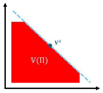
Figure 2: Illustration of Part 2)

Part 2) Prove for a stochastic policy class $\Pi$, we have $\Pi_{\mathrm{P}}^{*}\subseteq\{\pi~{}|~{}\pi\in\mathop{\mathrm{argmax}}_{\pi\in\Pi}\mathrm{LIN}_{\bm{\lambda}}(\pi),\forall\bm{\lambda}\in\Delta_{m}^{o}\}$ and $\Pi_{\mathrm{W}}^{*}\subseteq\{\pi~{}|~{}\pi\in\mathop{\mathrm{argmax}}_{\pi\in\Pi}\mathrm{LIN}_{\bm{\lambda}}(\pi),\forall\bm{\lambda}\in\Delta_{m}\}$. According to Proposition 4.1, we know that $\mathbb{V}(\Pi)$ is a convex polytope when $\Pi$ is a stochastic policy class.

Now we prove that if $\mathbb{V}(\Pi)$ is a convex polytope, any Pareto optimal policy can be the solution of $\max_{\pi}\mathrm{LIN}_{\bm{\lambda}}(\pi)$ for some $\bm{\lambda}\in\Delta_{m}^{o}$. It is equivalent to show that for any vector of value functions $\bm{V}^{0}=(V^{0}_{1},\dots,V^{0}_{m})\in\mathbb{V}(\Pi)$ with $\bm{V}^{0}=\bm{V}_{1}^{\pi_{0}}(s_{1})$ for a Pareto optimal policy $\pi_{0}\in\Pi_{\mathrm{P}}^{*}$, we have $\bm{V}^{0}=\mathop{\mathrm{argmax}}_{\bm{V}\in\mathbb{V}(\Pi)}\bm{\lambda}_{0}^{\top}\bm{V}$ and $\max_{\bm{V}\in\mathbb{V}(\Pi)}\bm{\lambda}_{0}^{\top}\bm{V}=\max_{\pi\in\Pi}\sum_{i=1}^{m}\bm{\lambda}_{0}^{\top}\bm{V}_{1}^{\pi}(s_{1})$ for some $\bm{\lambda}_{0}\in\Delta_{m}^{o}$. If there exists a hyperplane $\{\bm{V}\in\mathbb{R}^{m}~{}|~{}\sum_{i=1}^{m}a_{i}V_{i}=C\}$ satisfying $C\geq 0$, $a_{i}>0$, $\sum_{i=1}^{m}a_{i}V^{0}_{i}=C$ and $\mathbb{V}(\Pi)\subseteq\{\bm{V}\in\mathbb{R}^{m}~{}|~{}\sum_{i=1}^{m}a_{i}V_{i}\leq C\}$, then we have $\bm{V}^{0}=\mathop{\mathrm{argmax}}_{\bm{V}\in V(\Pi)}\sum_{i=1}^{m}a_{i}V_{i}$. Without loss of generality, we can assume that $\sum_{i=1}^{m}a_{i}=1$. Then, setting $\lambda_{i}=a_{i}$ leads to the desired result directly. As $\mathbb{V}(\Pi)$ is a convex polytope for the stochastic policy class $\Pi$, the boundary of it must be the combinations of some faces of this polytope. We denote these faces by $F_{i},i=1,\dots,n_{F}$, where $n_{F}$ is the number of faces. Correspondingly, the boundary of $\mathbb{V}(\Pi)$ is $\cup_{i=1}^{n_{F}}F_{i}$. As values for the Pareto front must be a subset of the boundary, for any $\bm{V}^{0}\in\mathbb{V}(\Pi_{\mathrm{P}}^{*})=\{\bm{V}_{1}^{\pi}(s_{1})~{}|~{}\pi\in\Pi_{\mathrm{P}}^{*}\}$, it must be on some face $F_{i}$. In other words, $\bm{V}^{0}\in F_{i}^{*}:=F_{i}\cap\mathbb{V}(\Pi_{\mathrm{P}}^{*})$ and $F_{i}^{*}$ is a face with dimension at most $m-1$. Consider the case that $F_{i}^{*}$ is an $(m-1)$-dimension face first. Suppose that the normal vector of the face is $(a_{1},a_{2},\dots,a_{m})$. Without loss of generality, we assume that $a_{1}>0$. Then, we must have $a_{i}>0$ for any $i>0$, leading to $C=\sum_{i=1}^{m}a_{i}V_{i}^{0}\geq 0$. Otherwise, supposing that $a_{2}\leq 0$, we can find two points $\bm{V}^{1}$ and $\bm{V}^{2}$ on $F_{i}^{*}$ such that $\sum_{i=1}^{m}a_{i}V_{i}^{1}=\sum_{i=1}^{m}a_{i}V_{i}^{2}$ with $V^{1}_{1}\geq V^{2}_{1}$, $V^{1}_{2}>V^{2}_{2}$ and $V^{1}_{i}=V^{2}_{i}$ for $i>2$, implying $\bm{V}^{2}$ does not correspond to a Pareto optimal policy. It contradicts the fact that the face corresponds to the Pareto front. Therefore, when the dimension of $F_{i}^{*}$ is $m-1$, $F_{i}^{*}$ satisfies $a_{i}>0$ and the convexity of the polytope implies that $\{\bm{V}\in\mathbb{R}^{m}~{}|~{}\sum_{i=1}^{m}a_{i}V_{i}\leq C\}$. Thus, the hyperplane we need is directly the one that $F_{i}^{*}$ lies on. If the dimension of $F_{i}^{*}$ is smaller than $m-1$, similarly, we could find a $m-1$-dimension hyperplane such that the $F_{i}^{*}$ is on that plane and $\mathbb{V}(\Pi)\subseteq\{\bm{V}\in\mathbb{R}^{m}|\sum_{i=1}^{m}a_{i}V_{i}\leq C\}$. The above construction is illustrated in Figure 2. This completes the proof of $\Pi_{\mathrm{P}}^{*}\subseteq\{\pi~{}|~{}\pi\in\mathop{\mathrm{argmax}}_{\pi\in\Pi}\mathrm{LIN}_{\bm{\lambda}}(\pi),\forall\bm{\lambda}\in\Delta_{m}^{o}\}$.

Following the same spirit, we could show that $\Pi_{\mathrm{W}}^{*}\subseteq\{\pi~{}|~{}\pi\in\mathop{\mathrm{argmax}}_{\pi\in\Pi}\mathrm{LIN}_{\bm{\lambda}}(\pi),\forall\bm{\lambda}\in\Delta_{m}\}$. In fact, it is sufficient to show that for any weak Pareto optimal policy $\pi_{0}\in\Pi_{\mathrm{W}}^{*}$ and the corresponding value function $\bm{V}^{0}$, there exists a hyperplane $\{\bm{V}\in\mathbb{R}^{m}~{}|~{}\sum_{i=1}^{m}a_{i}V_{i}=C\}$ satisfying $C\geq 0$, $a_{i}\geq 0$, $\sum_{i=1}^{m}a_{i}V^{0}_{i}=C$ and $\mathbb{V}(\Pi)\subseteq\{\bm{V}\in\mathbb{R}^{m}~{}|~{}\sum_{i=1}^{m}a_{i}V_{i}\leq C\}$. In other words, we relax the condition $a_{i}>0$ in the above proof to $a_{i}\geq 0$ for weak Pareto points. The proof is similar to that of $\Pi_{\mathrm{P}}^{*}\subseteq\{\pi~{}|~{}\pi\in\mathop{\mathrm{argmax}}_{\pi\in\Pi}\mathrm{LIN}_{\bm{\lambda}}(\pi),\forall\bm{\lambda}\in\Delta_{m}^{o}\}$. Specifically, for a weak Pareto point $\bm{V}^{0}\in\breve{F}_{i}^{*}:=F_{i}\cap\mathbb{V}(\Pi_{\mathrm{W}})^{*}$, if $\breve{F}_{i}^{*}$ is a face of dimension $m-1$, the normal vector of it satisfies $a_{i}\geq 0$. If we assume that $a_{i}\geq 0$ for $i\in\mathcal{I}^{+}$ and $a_{j}<0$ for $j\in[m]\backslash\mathcal{I}^{+}$, we can find two points $\bm{V}^{1}$ and $\bm{V}^{2}$ on $\breve{F}_{i}^{*}$ such that $\sum_{i=1}^{m}a_{i}V_{i}^{1}=\sum_{i=1}^{m}a_{i}V_{i}^{2}$ with $V_{i}^{2}=V_{i}^{1}+\epsilon_{i}$ for $i\in\mathcal{I}^{+}$ and $V_{j}^{2}=V_{j}^{1}+\epsilon_{j}$ for $j\in[m]\backslash\mathcal{I}^{+}$ where $\epsilon_{i}\geq 0$ for all $i\in[m]$. This requires $\sum_{i\in\mathcal{I}^{+}}a_{i}\epsilon_{i}=\sum_{j\in[m]\backslash\mathcal{I}^{+}}(-a_{j})\epsilon_{j}$. Supposing we have at least one $i\in\mathcal{I}^{+}$ such that $a_{i}>0$ (we let $\sum_{i=1}^{m}a_{i}=1$ without loss of generality), we can find sufficiently small positive $\epsilon_{i}$ for all $i\in[m]$ that satisfy $\sum_{i\in\mathcal{I}^{+}}a_{i}\epsilon_{i}=\sum_{j\in[m]\backslash\mathcal{I}^{+}}(-a_{j})\epsilon_{j}$, which implies $V_{i}^{1}>V_{i}^{2}$ for all $i\in[m]$, or equivalently $\bm{V}^{2}$ does not correspond to a weakly Pareto optimal policy according to Definition 3.3. This contradicts the fact that all the values on the face correspond to weak Pareto optimal policies. The remaining proof is exactly the same as that for $\Pi_{\mathrm{P}}^{*}\subseteq\{\pi~{}|~{}\pi\in\mathop{\mathrm{argmax}}_{\pi\in\Pi}\mathrm{LIN}_{\bm{\lambda}}(\pi),\forall\bm{\lambda}\in\Delta_{m}^{o}\}$.

Part 3) Now we use a concrete example to illustrate that for a deterministic policy class $\Pi$, a Pareto optimal policy may not be the solution of $\max_{\pi\in\Pi}\bm{\lambda}^{\top}\bm{V}_{1}^{\pi}(s_{1})$ for any $\bm{\lambda}\in\Delta_{m}$. We consider a multi-objective multi-arm bandit problem, a simple and special MOMDP whose state space size $|{\mathcal{S}}|=1$, episode length $H=1$, with a deterministic policy. Here we assume this bandit problem has $m=2$ reward functions $r_{1}$ and $r_{2}$ and $|\mathcal{A}|=4$ actions. We define

$$r_{1}(a_{1})=1,\quad r_{1}(a_{2})=0.5,\quad r_{1}(a_{3})=0.6,\quad r_{1}(a_{4})=0.65,$$

$$r_{2}(a_{1})=0,\quad r_{2}(a_{2})=0.5,\quad r_{2}(a_{3})=0.2,\quad r_{2}(a_{4})=0.3,$$

which are the reward values of the four actions for each reward function. Via the definition of the Pareto optimal policy, we can identify that $a_{1}$, $a_{2}$, and $a_{4}$ are the Pareto optimal policy, or Pareto optimal arms in a multi-arm bandit problem.

Letting $0\leq\lambda\leq 1$, we generate a reward function as a linear combination of $r_{1}$ and $r_{2}$ via $\lambda$ and $1-\lambda$, i.e., $r_{\lambda}(a):=\lambda r_{1}(a)+(1-\lambda)r_{2}(a)$, such that

$$r_{\lambda}(a_{1})=\lambda,\quad r_{\lambda}(a_{2})=0.5,\quad r_{\lambda}(a_{3})=0.2+0.4\lambda,\quad r_{\lambda}(a_{4})=0.3+0.35\lambda.$$

Then we have:

• when $\lambda<0.5$, we have $a_{2}=\mathop{\mathrm{argmax}}_{a}r_{\lambda}(a)$,

• when $\lambda=0.5$, we have $a_{1},a_{2}=\mathop{\mathrm{argmax}}_{a}r_{\lambda}(a)$,

• when $\lambda>0.5$, we have $a_{1}=\mathop{\mathrm{argmax}}_{a}r_{\lambda}(a)$.

Therefore, we only find $a_{1}$ and $a_{2}$ as the solutions for any $\lambda$, which are also Pareto optimal arms. However, the Pareto optimal arm $a_{3}$ is not identified by solving $\max_{a}r_{\lambda}(a)$, for all $0\leq\lambda\leq 1$, which completes the example for the second claim. The proof of this proposition is completed. ∎

B.3 Proof of Proposition 4.4

Following the proof in [Jiang et al., 2023] that focuses on a general online convex minimization problem, we present our proof specializing in the multi-objective RL maximization problem.

Proof.

By Definition 4.3, we can rewrite the Pareto suboptimality gap $\mathrm{PSG}$ as follows:

$$\begin{aligned} &\mathrm{PSG}(\pi):=\sup_{\pi^{*}\in\Pi_{\mathrm{P}}^{*}}\mathop{\mathrm{inf}\vphantom{\mathrm{sup}}}_{\epsilon(\pi^{*})\geq 0}\epsilon(\pi^{*}),\\ &\text{s.t.}~{}~{}~{}~{}~{}~{}\exists i\in[m],~{}V_{i,1}^{\pi}(s_{1})+\epsilon(\pi^{*})>V_{i,1}^{\pi^{*}}(s_{1}),\\ &~{}~{}~{}~{}~{}\textbf{or}~{}~{}\forall i\in[m],~{}V_{i,1}^{\pi}(s_{1})+\epsilon(\pi^{*})=V_{i,1}^{\pi^{*}}(s_{1}).\end{aligned}$$ (27)

If $\exists i\in[m]$, $V_{i,1}^{\pi}(s_{1})\geq V_{i,1}^{\pi^{*}}(s_{1})$ for a policy $\pi^{*}\in\Pi_{\mathrm{P}}^{*}$, then the policy $\pi$ satisfies either of the following cases:

• $\exists i\in[m]$, $V_{i,1}^{\pi}(s_{1})=V_{i,1}^{\pi^{*}}(s_{1})$,

• $\forall i\in\mathcal{I}\subset[m]$, $V_{i,1}^{\pi}(s_{1})>V_{i,1}^{\pi^{*}}(s_{1})$ and $\forall j\in[m]\backslash\mathcal{I}$, $V_{j,1}^{\pi}(s_{1})<V_{i,1}^{\pi^{*}}(s_{1})$.

Case (a) indicates that $\epsilon(\pi^{*})>0$ satisfies the above constraint in (LABEL:eq:subopt-eqform), implying that $\inf_{\epsilon(\pi^{*})>0}\epsilon(\pi^{*})=0$. On the other hand, case (b) indicates that $\epsilon(\pi^{*})=0$ satisfies the constraint in (LABEL:eq:subopt-eqform), thus implying that $\inf_{\epsilon(\pi^{*})=0}\epsilon(\pi^{*})=0$.

If $\forall i\in[m]$, $V_{i,1}^{\pi}(s_{1})<V_{i,1}^{\pi^{*}}(s_{1})$ for a policy $\pi^{*}\in\Pi_{\mathrm{P}}^{*}$, then we have $\epsilon(\pi^{*})=\min_{i}(V_{i,1}^{\pi^{*}}(s_{1})-V_{i,1}^{\pi}(s_{1}))$ such that $\inf_{\epsilon(\pi^{*})\geq 0}\epsilon(\pi^{*})=\min_{i}(V_{i,1}^{\pi^{*}}(s_{1})-V_{i,1}^{\pi}(s_{1}))=\inf_{\bm{\lambda}^{*}\in\Delta_{m}}\bm{\lambda}^{*}{}^{\top}(\bm{V}_{1}^{\pi^{*}}(s_{1})-\bm{V}_{1}^{\pi}(s_{1}))>0$, where $\Delta_{m}:=\{\bm{\lambda}=(\lambda_{i})_{i=1}^{m}\in\mathbb{R}^{m}~{}|~{}\sum_{i=1}^{m}\lambda_{i}=1,\lambda_{i}\geq 0\}$ is a simplex in $\mathbb{R}^{m}$.

Overall, we know that for any policy $\pi\in\Pi$, the Pareto suboptimality gap is equivalent to

$$\mathrm{PSG}(\pi):=\sup_{\pi^{*}\in\Pi_{\mathrm{P}}^{*}}\mathop{\mathrm{inf}\vphantom{\mathrm{sup}}}_{\epsilon(\pi^{*})\geq 0}\epsilon(\pi^{*})=\sup_{\pi^{*}\in\Pi_{\mathrm{P}}^{*}}\mathop{\mathrm{inf}\vphantom{\mathrm{sup}}}_{\bm{\lambda}^{*}\in\Delta_{m}}\bm{\lambda}^{*}{}^{\top}(\bm{V}_{1}^{\pi^{*}}(s_{1})-\bm{V}_{1}^{\pi}(s_{1})).$$

This completes the proof of Proposition 4.4 ∎

B.4 Proof of Proposition 4.5

Proof.

The proof of this proposition is divided into two parts: we first prove that $\pi\in\Pi_{\mathrm{W}}^{*}$ implies $\mathrm{PSG}(\pi)=0$; then we show that $\mathrm{PSG}(\pi)=0$ implies $\pi$ is weakly Pareto optimal. Recall that the definition of $\mathrm{PSG}$ is

$$\begin{aligned} &\mathrm{PSG}(\pi):=\inf_{\epsilon\geq 0}\epsilon,\\ &\text{s.t.}~{}~{}\forall\pi^{*}\in\Pi_{\mathrm{P}}^{*},\exists i\in[m],V_{i,1}^{\pi}(s_{1})+\epsilon>V_{i,1}^{\pi^{*}}(s_{1}),\\ &\qquad\qquad~{}~{}~{}\text{or}~{}~{}\forall i\in[m],V_{i,1}^{\pi}(s_{1})+\epsilon=V_{i,1}^{\pi^{*}}(s_{1}).\end{aligned}$$ (28)

And we say a policy $\pi$ is not dominated by $\pi^{\prime}$ if and only if

$$\exists i\in[m],~{}~{}V_{i,1}^{\pi}(s_{1})>V_{i,1}^{\pi^{\prime}}(s_{1}),$$ (29)

or $$\forall i\in[m],~{}~{}V_{i,1}^{\pi}(s_{1})=V_{i,1}^{\pi^{\prime}}(s_{1}).$$ (30)

Part 1) Prove $\pi\in\Pi_{\mathrm{W}}^{*}\Rightarrow\mathrm{PSG}(\pi)=0$. By the definition of weak Pareto optimality, for $\pi\in\Pi_{\mathrm{W}}^{*}$, we have for all $\pi^{\prime}$,

$$\exists i\in[m],\quad V_{i,1}^{\pi}(s_{1})\geq V_{i,1}^{\pi^{\prime}}(s_{1}).$$

Letting $\pi^{\prime}=\pi^{*}\in\Pi_{\mathrm{P}}^{*}$, we have for all $\pi^{*}\in\Pi_{\mathrm{P}}^{*}$, $\exists i\in[m],V_{i,1}^{\pi}(s_{1})\geq V_{i,1}^{\pi^{*}}(s_{1})$. Therefore, we have for any $\epsilon>0$, $\forall\pi^{*}\in\Pi_{\mathrm{P}}^{*}$, $\exists i\in[m],V_{i,1}^{\pi}(s_{1})+\epsilon>V_{i,1}^{\pi^{*}}(s_{1})$, which satisfies the constraint in (LABEL:eq:so-recall). Then, for $\pi\in\Pi_{\mathrm{W}}^{*}$, $\mathrm{PSG}(\pi)=\inf_{\epsilon>0}\epsilon=0$, which completes the proof of Part 1).

Part 2) Prove $\mathrm{PSG}(\pi)=0\Rightarrow\pi$ is weakly Pareto optimal. $\mathrm{PSG}(\pi)=0$ indicates that the zero value is achieved at either $\epsilon=0$ or arbitrarily small $\epsilon\rightarrow 0^{+}$ with $\epsilon>0$ (due to $\inf_{\epsilon>0}\epsilon=0$).

When it is achieved at $\epsilon=0$, by (LABEL:eq:so-recall), we have that $\pi$ satisfies

$$\forall\pi^{*}\in\Pi_{\mathrm{P}}^{*},~{}~{}\exists i\in[m],V_{i,1}^{\pi}(s_{1})>V_{i,1}^{\pi^{*}}(s_{1}),\quad\text{or}\quad\forall i\in[m],V_{i,1}^{\pi}(s_{1})=V_{i,1}^{\pi^{*}}(s_{1}).$$

By (29) and (30), it implies that $\pi$ is not dominated by any $\pi^{*}\in\Pi_{\mathrm{P}}^{*}$. Further employing the property of the Pareto set that $\pi\in\Pi_{\mathrm{P}}^{*}$ if and only if $\pi$ is not dominated by any $\pi^{*}\in\Pi_{\mathrm{P}}^{*}$ as in Property 3.2, we know that the policy $\pi$ is a Pareto optimal policy in $\Pi_{\mathrm{P}}^{*}$ for when $\epsilon=0$.

On the other hand, when $\mathrm{PSG}(\pi)=0$ is achieved at arbitrarily small $\epsilon$ with $\epsilon>0$, the constraint in (LABEL:eq:so-recall) is equivalent to

$$\forall\pi^{*}\in\Pi_{\mathrm{P}}^{*},\exists i\in[m],V_{i,1}^{\pi}(s_{1})\geq V_{i,1}^{\pi^{*}}(s_{1}),$$ (31)

since no policy $\pi$ satisfies the second constraint in (LABEL:eq:so-recall) that $\forall i\in[m],V_{i,1}^{\pi}(s_{1})+\epsilon=V_{i,1}^{\pi^{*}}(s_{1})$ for an arbitrarily small $\epsilon$. In addition, according to (a) of Property 3.2, we have that

$$\forall\pi^{\prime}\notin\Pi_{\mathrm{P}}^{*},\exists\pi^{*}\in\Pi_{\mathrm{P}}^{*},\forall i\in[m],V_{i,1}^{\pi^{*}}(s_{1})\geq V_{i,1}^{\pi^{\prime}}(s_{1}),$$

according to the definition of dominance in Definition 3.1. Therefore, we construct a minimal subset $\widetilde{\Pi}^{*}\subset\Pi_{\mathrm{P}}^{*}$ that all policies in $\widetilde{\Pi}^{*}$ can dominate at least one policy outside $\Pi_{\mathrm{P}}^{*}$ and the rest of policies in $\Pi_{\mathrm{P}}^{*}\backslash\widetilde{\Pi}^{*}$ dominates no policy, which gives

$$\forall\pi^{\prime}\notin\Pi_{\mathrm{P}}^{*},\exists\pi^{*}\in\widetilde{\Pi}^{*},\forall i\in[m],V_{i,1}^{\pi^{*}}(s_{1})\geq V_{i,1}^{\pi^{\prime}}(s_{1}).$$

Thus, combining it with (31), if $\mathrm{PSG}(\pi)=0$ is achieved at arbitrarily small $\epsilon$, we have

$$\forall\pi^{\prime}\notin\Pi_{\mathrm{P}}^{*},\exists i\in[m],V_{i,1}^{\pi}(s_{1})\geq V_{i,1}^{\pi^{\prime}}(s_{1}).$$

Furthermore, combining (31) with the above equation, we have

$$\forall\pi^{\prime},\exists i\in[m],V_{i,1}^{\pi}(s_{1})\geq V_{i,1}^{\pi^{\prime}}(s_{1}),$$

which indicates that $\pi$ satisfies

$$\nexists\pi^{\prime},\forall i\in[m],V_{i,1}^{\pi}(s_{1})<V_{i,1}^{\pi^{\prime}}(s_{1}).$$

Further by Definition 3.3, $\pi$ is weakly Pareto optimal.

Jointly considering the cases of $\epsilon=0$ and $\epsilon$ being arbitrarily small, we eventually prove that $\mathrm{PSG}(\pi)=0$ implies $\pi$ is weakly Pareto optimal. The proof of Proposition 4.5 is completed by combining the results in Part 1) and Part 2). ∎

B.5 Proof of Proposition 4.7

Proof.

We revisit the proofs in prior works on Tchebycheff scalarization for multi-objective optimization, e.g., Choo and Atkins [1983], Ehrgott [2005]. We adapt their proofs to the MORL setting and present them here for completeness.

The proof of the first claim in this proposition is divided into two parts: we first prove $\pi_{\bm{\lambda}}^{*}\in\mathop{\mathrm{argmin}}_{\pi\in\Pi}\mathrm{TCH}_{\bm{\lambda}}(\pi)$ for a $\bm{\lambda}\in\Delta_{m}$ $\Rightarrow\pi_{\bm{\lambda}}^{*}$ is weakly Pareto optimal; then we prove $\breve{\pi}$ is weakly Pareto optimal $\Rightarrow\breve{\pi}\in\mathop{\mathrm{argmin}}_{\pi\in\Pi}\mathrm{TCH}_{\bm{\lambda}}(\pi)$ for some $\bm{\lambda}\in\Delta_{m}$.

Part 1) Prove $\pi_{\bm{\lambda}}^{*}\in\mathop{\mathrm{argmin}}_{\pi\in\Pi}\mathrm{TCH}_{\bm{\lambda}}(\pi)$ for a $\bm{\lambda}\in\Delta_{m}^{o}$ $\Rightarrow\pi_{\bm{\lambda}}^{*}$ is weakly Pareto optimal. This is equivalent to showing that the solutions to $\mathop{\mathrm{minimize}}_{\pi\in\Pi}\mathrm{TCH}_{\bm{\lambda}}(\pi)$ for all $\bm{\lambda}$ are weakly Pareto optimal.

Since for a given $\bm{\lambda}$ we have $\pi_{\bm{\lambda}}^{*}\in\mathop{\mathrm{argmin}}_{\pi\in\Pi}\mathrm{TCH}_{\bm{\lambda}}(\pi)$, then by the definition of $\mathrm{TCH}_{\bm{\lambda}}(\pi)$ in Definition 4.6, we know that

$$\max_{i}\{\lambda_{i}(V_{i,1}^{*}(s_{1})+\iota-V_{i,1}^{\pi_{\bm{\lambda}}^{*}}(s_{1}))\}=\min_{\pi\in\Pi}\max_{i}\{\lambda_{i}(V_{i,1}^{*}(s_{1})+\iota-V_{i,1}^{\pi}(s_{1}))\},$$

which indicates that

$$\max_{i}\{\lambda_{i}(V_{i,1}^{*}(s_{1})+\iota-V_{i,1}^{\pi_{\bm{\lambda}}^{*}}(s_{1}))\}\leq\max_{i}\{\lambda_{i}(V_{i,1}^{*}(s_{1})+\iota-V_{i,1}^{\pi}(s_{1}))\},\quad\forall\pi\in\Pi.$$ (32)

Now we prove by contradiction that $\pi_{\bm{\lambda}}^{*}$ is weakly Pareto optimal. If $\pi_{\bm{\lambda}}^{*}$ is not weakly Pareto optimal, then by Definition 3.3, we know that there exists another policy $\pi^{\prime}\in\Pi$ satisfying $V_{i,1}^{\pi_{\bm{\lambda}}^{*}}(s_{1})<V_{i,1}^{\pi^{\prime}}(s_{1})$ for all $i\in[m]$, which means that

$$\exists\pi^{\prime},\lambda_{i}(V_{i,1}^{*}(s_{1})+\iota-V_{i,1}^{\pi_{\bm{\lambda}}^{*}}(s_{1}))>\lambda_{i}(V_{i,1}^{*}(s_{1})+\iota-V_{i,1}^{\pi^{\prime}}(s_{1})).$$

Given that $\bm{\lambda}\in\Delta_{m}^{o}$, we further have

$$\max_{i\in[m]}\{\lambda_{i}(V_{i,1}^{*}(s_{1})+\iota-V_{i,1}^{\pi_{\bm{\lambda}}^{*}}(s_{1}))\}>\max_{i\in[m]}\{\lambda_{i}(V_{i,1}^{*}(s_{1})+\iota-V_{i,1}^{\pi^{\prime}}(s_{1}))\},$$

which contradicts (32) that $\max_{i}\{\lambda_{i}(V_{i,1}^{*}(s_{1})+\iota-V_{i,1}^{\pi_{\bm{\lambda}}^{*}}(s_{1}))\}\leq\max_{i}\{\lambda_{i}(V_{i,1}^{*}(s_{1})+\iota-V_{i,1}^{\pi^{\prime}}(s_{1}))\}$. Therefore, $\pi_{\bm{\lambda}}^{*}$ is a weakly Pareto optimal policy.

Part 2) Prove $\breve{\pi}$ is weakly Pareto optimal $\Rightarrow\breve{\pi}=\mathop{\mathrm{argmin}}_{\pi\in\Pi}\mathrm{TCH}_{\bm{\lambda}}(\pi)$ for some $\bm{\lambda}\in\Delta_{m}^{o}$. This is equivalent to showing that if $\breve{\pi}$ is weakly Pareto optimal, then we can find a $\bm{\lambda}$ such that $\breve{\pi}$ is a minimizer of the problem $\mathop{\mathrm{minimize}}_{\pi\in\Pi}\mathrm{TCH}_{\bm{\lambda}}(\pi)$.

For the policy $\breve{\pi}$, we let $\bm{\lambda}$ be

$$\lambda_{i}=\frac{(V_{i,1}^{*}(s_{1})+\iota-V_{i,1}^{\breve{\pi}}(s_{1}))^{-1}}{\sum_{j=1}^{m}(V_{j,1}^{*}(s_{1})+\iota-V_{j,1}^{\breve{\pi}}(s_{1}))^{-1}}>0,$$

where $V_{j,1}^{*}(s_{1})+\iota-V_{j,1}^{\breve{\pi}}(s_{1})>0$ always holds, and we have $\lambda_{i}(V_{i,1}^{*}(s_{1})+\iota-V_{i,1}^{\breve{\pi}}(s_{1}))=\lambda_{i^{\prime}}(V_{i^{\prime},1}^{*}(s_{1})+\iota-V_{i^{\prime},1}^{\breve{\pi}}(s_{1}))=[\sum_{j=1}^{m}(V_{j,1}^{*}(s_{1})+\iota-V_{j,1}^{\breve{\pi}}(s_{1}))^{-1}]^{-1}$ for all $i\neq i^{\prime}$ such that

$$\mathrm{TCH}_{\bm{\lambda}}(\breve{\pi})=\lambda_{i}(V_{i,1}^{*}(s_{1})+\iota-V_{i,1}^{\breve{\pi}}(s_{1})),\quad\forall i\in[m].$$

Next, we show that if $\breve{\pi}$ is weakly Pareto optimal, then $\breve{\pi}$ minimizes the function $\mathrm{TCH}_{\bm{\lambda}}(\pi)$ with $\bm{\lambda}$ defined above. We prove this claim by contradiction. If there exists another policy $\pi^{\prime}$ satisfying $\mathrm{TCH}_{\bm{\lambda}}(\pi^{\prime})<\mathrm{TCH}_{\bm{\lambda}}(\breve{\pi})$, we have

$$\max_{j\in[m]}\{\lambda_{j}(V_{j,1}^{*}(s_{1})+\iota-V_{j,1}^{\pi^{\prime}}(s_{1}))\}<\mathrm{TCH}_{\bm{\lambda}}(\breve{\pi})=\lambda_{i}(V_{i,1}^{*}(s_{1})+\iota-V_{i,1}^{\breve{\pi}}(s_{1})),\quad\forall i\in[m],$$

which further implies that

$$\lambda_{i}(V_{i,1}^{*}(s_{1})+\iota-V_{i,1}^{\pi^{\prime}}(s_{1}))<\lambda_{i}(V_{i,1}^{*}(s_{1})+\iota-V_{i,1}^{\breve{\pi}}(s_{1})),\quad\forall i\in[m].$$

The above inequality means that $\breve{\pi}$ is not a weakly Pareto optimal according to Definition 3.3, which contradicts the premise that $\breve{\pi}$ is a weakly Pareto optimal. Therefore, we can prove Part 2). This completes the first claim of this proposition.

Now we prove the second claim of this proposition by contradiction. Let $\breve{\pi}:=\mathop{\mathrm{argmin}}_{\pi\in\Pi}\mathrm{TCH}_{\bm{\lambda}}(\pi)$ for a $\bm{\lambda}$. Assume that $\breve{\pi}$ is not Pareto optimal. According to the definition of the Pareto optimal policy in Definition 3.1, we have that there exists a policy $\pi\neq\breve{\pi}$ such that

$$V_{i,1}^{\breve{\pi}}(s_{1})\leq V_{i,1}^{\pi}(s_{1}),~{}\forall i\in[m].$$

According to the definition of $\mathrm{TCH}_{\bm{\lambda}}$, the above inequality leads to

$$\mathrm{TCH}_{\bm{\lambda}}(\pi)\leq\mathrm{TCH}_{\bm{\lambda}}(\breve{\pi}).$$

However, since $\breve{\pi}$ is the only solution to $\mathrm{TCH}_{\bm{\lambda}}(\pi)$, we have $\mathrm{TCH}_{\bm{\lambda}}(\pi)>\mathrm{TCH}_{\bm{\lambda}}(\breve{\pi})$, which contradicts the above inequality that $\mathrm{TCH}_{\bm{\lambda}}(\pi)\leq\mathrm{TCH}_{\bm{\lambda}}(\breve{\pi})$. This completes our proof of Proposition 4.7. ∎

B.6 Proof of Proposition 4.8

Proposition B.1.

There always exists a subset $\Lambda\subseteq\Delta_{m}$ such that $\{\pi~{}|~{}\pi\in\min_{\pi\in\Pi}\mathrm{TCH}_{\bm{\lambda}}(\pi),\forall\bm{\lambda}\in\Lambda\subseteq\Delta_{m}^{o}\}=\Pi_{\mathrm{P}}^{*}$. Supposing that $\pi_{\bm{\lambda}}^{*}$ is one arbitrary solution to $\min_{\pi\in\Pi}\mathrm{TCH}_{\bm{\lambda}}(\pi)$, for each $\bm{\lambda}\in\Lambda$, all the solutions to $\min_{\pi\in\Pi}\mathrm{TCH}_{\bm{\lambda}}(\pi)$ is Pareto optimal with the same value $V_{i,1}^{\pi_{\bm{\lambda}}^{*}}(s_{1})$ for all $i\in[m]$.

Proof.

For each $\pi\in\Pi_{\mathrm{P}}^{*}$, we set the associated $\bm{\lambda}$ as

$$\lambda_{i}=\frac{(V_{i,1}^{*}(s_{1})+\iota-V_{i,1}^{\pi}(s_{1}))^{-1}}{\sum_{j=1}^{m}(V_{j,1}^{*}(s_{1})+\iota-V_{j,1}^{\pi}(s_{1}))^{-1}}>0.$$

Then we can define the set

$$\Lambda:=\left\{\bm{\lambda}~{}:~{}\lambda_{i}=\frac{(V_{i,1}^{*}(s_{1})+\iota-V_{i,1}^{\pi}(s_{1}))^{-1}}{\sum_{j=1}^{m}(V_{j,1}^{*}(s_{1})+\iota-V_{j,1}^{\pi}(s_{1}))^{-1}},~{}~{}\forall\pi\in\Pi_{\mathrm{P}}^{*}\right\}.$$

Now we first show $\Pi_{\mathrm{P}}^{*}\subseteq\{\pi~{}|~{}\pi\in\min_{\pi\in\Pi}\mathrm{TCH}_{\bm{\lambda}}(\pi),\forall\bm{\lambda}\in\Lambda\subseteq\Delta_{m}^{o}\}$. According to Part 2) of the proof of Proposition 4.7 in the subsection above, we can show for any $\breve{\pi}\in\Pi_{\mathrm{P}}^{*}\subseteq\Pi_{\mathrm{W}}^{*}$, it is the solution to the problem $\min_{\pi\in\Pi}\mathrm{TCH}_{\bm{\lambda}}(\pi)$ with $\lambda_{i}=\frac{(V_{i,1}^{*}(s_{1})+\iota-V_{i,1}^{\breve{\pi}}(s_{1}))^{-1}}{\sum_{j=1}^{m}(V_{j,1}^{*}(s_{1})+\iota-V_{j,1}^{\breve{\pi}}(s_{1}))^{-1}}$. Thus, we conclude $\Pi_{\mathrm{P}}^{*}\subseteq\{\pi~{}|~{}\pi\in\min_{\pi\in\Pi}\mathrm{TCH}_{\bm{\lambda}}(\pi),\forall\bm{\lambda}\in\Lambda\subseteq\Delta_{m}^{o}\}$.

Next, we prove $\{\pi~{}|~{}\pi\in\min_{\pi\in\Pi}\mathrm{TCH}_{\bm{\lambda}}(\pi),\forall\bm{\lambda}\in\Lambda\subseteq\Delta_{m}^{o}\}\subseteq\Pi_{\mathrm{P}}^{*}$ and all solutions of $\min_{\pi\in\Pi}\mathrm{TCH}_{\bm{\lambda}}(\pi)$ for each $\bm{\lambda}\in\Lambda$ has the same value. Since the uniqueness of the solution to $\min_{\pi\in\Pi}\mathrm{TCH}_{\bm{\lambda}}(\pi)$ leads to Pareto optimality according to Proposition 4.7, we now assume $\min_{\pi\in\Pi}\mathrm{TCH}_{\bm{\lambda}}(\pi)$ has more than one solution. We assume $\widetilde{\pi}$ is one solution to $\min_{\pi\in\Pi}\mathrm{TCH}_{\bm{\lambda}}(\pi)$ under some $\bm{\lambda}$ with $\lambda_{i}=\frac{(V_{i,1}^{*}(s_{1})+\iota-V_{i,1}^{\breve{\pi}}(s_{1}))^{-1}}{\sum_{j=1}^{m}(V_{j,1}^{*}(s_{1})+\iota-V_{j,1}^{\breve{\pi}}(s_{1}))^{-1}}$ for some $\breve{\pi}\in\Pi_{\mathrm{P}}^{*}$. According to the above proof, we know that $\breve{\pi}$ is also the solution to the problem $\min_{\pi\in\Pi}\mathrm{TCH}_{\bm{\lambda}}(\pi)$. Now we further assume that $\widetilde{\pi}\neq\breve{\pi}$. Since $\breve{\pi}\in\Pi_{\mathrm{P}}^{*}$, if we can show $V_{i,1}^{\widetilde{\pi}}(s_{1})=V_{i,1}^{\breve{\pi}}(s_{1}),\forall i\in[m]$, then we obtain $\widetilde{\pi}\in\Pi_{\mathrm{P}}$, which will complete the proof. We prove it by contradiction. Since $\breve{\pi}$ is a solution, we have

$$\min_{\pi}\mathrm{TCH}_{\bm{\lambda}}(\pi)=\mathrm{TCH}_{\bm{\lambda}}(\breve{\pi})=\frac{1}{\sum_{j=1}^{m}(V_{j,1}^{*}(s_{1})+\iota-V_{j,1}^{\breve{\pi}}(s_{1}))^{-1}}.$$

Then, we discuss different cases:

• If there exists $i^{\prime}$ such that $V_{i^{\prime},1}^{\widetilde{\pi}}(s_{1})<V_{i^{\prime},1}^{\breve{\pi}}(s_{1})$, then $\mathrm{TCH}_{\bm{\lambda}}(\widetilde{\pi})>\min_{\pi}\mathrm{TCH}_{\bm{\lambda}}(\pi)$, contradicting the assumption that $\widetilde{\pi}\in\mathop{\mathrm{argmin}}_{\pi}\mathrm{TCH}_{\bm{\lambda}}(\pi)$. Thus, we must have $V_{i,1}^{\widetilde{\pi}}(s_{1})\geq V_{i,1}^{\breve{\pi}}(s_{1}),~{}\forall i\in[m]$.

• If there exists $i^{\prime}$ such that $V_{i^{\prime},1}^{\widetilde{\pi}}(s_{1})>V_{i^{\prime},1}^{\breve{\pi}}(s_{1})$ with $V_{i,1}^{\widetilde{\pi}}(s_{1})=V_{i,1}^{\breve{\pi}}(s_{1})$ for other $i\neq i^{\prime}$, then by Definition 3.1, we know $\widetilde{\pi}$ dominates $\breve{\pi}$, implying that $\breve{\pi}$ is not Pareto optimal, which contradicts $\breve{\pi}\in\Pi_{\mathrm{P}}$.

By the above analysis, we obtain $V_{i,1}^{\widetilde{\pi}}(s_{1})=V_{i,1}^{\breve{\pi}}(s_{1}),\forall i\in[m]$ and $\widetilde{\pi}\in\Pi_{\mathrm{P}}$. The proof is completed. ∎

Appendix C Proofs for Section 5

This section provides detailed proofs of Proposition 5.1 and Theorem 5.2 along with several important lemmas for this theorem.

C.1 Proof of Proposition 5.1

Proof.

According to (4), we have

$$\mathrm{TCH}_{\bm{\lambda}}(\pi):=\max_{i\in[m]}\{\lambda_{i}(V_{i,1}^{*}(s_{1})+\iota-V_{i,1}^{\pi}(s_{1}))\}.$$

For any $x_{i}$, the inequality $\max_{i\in[m]}\{x_{i}\}=\max_{(w_{i})_{i=1}^{m}\in\Delta_{m}}\sum_{i=1}^{m}w_{i}x_{i}$ always holds. Thus, we obtain

$$\mathrm{TCH}_{\bm{\lambda}}(\pi)=\max_{(w_{i})_{i=1}^{m}\in\Delta_{m}}\sum_{i=1}^{m}w_{i}\lambda_{i}(V_{i,1}^{*}(s_{1})+\iota-V_{i,1}^{\pi}(s_{1})).$$

Moreover, we have $V_{i,1}^{*}(s_{1}):=\max_{\pi\in\Pi}V_{i,1}^{\pi}(s_{1})$ by its definition. Therefore, we eventually obtain that

$$\mathrm{TCH}_{\bm{\lambda}}(\pi) =\max_{(w_{i})_{i=1}^{m}\in\Delta_{m}}\sum_{i=1}^{m}w_{i}\lambda_{i}(\max_{\{\nu_{i}\in\Pi\}_{i=1}^{m}}V_{i,1}^{\nu_{i}}(s_{1})+\iota-V_{i,1}^{\pi}(s_{1}))$$

$$=\max_{(w_{i})_{i=1}^{m}\in\Delta_{m}}\max_{\{\nu_{i}\in\Pi\}_{i=1}^{m}}\sum_{i=1}^{m}w_{i}\lambda_{i}(V_{i,1}^{\nu_{i}}(s_{1})+\iota-V_{i,1}^{\pi}(s_{1})).$$

This completes the proof. ∎

C.2 Lemmas for Theorem 5.2

Lemma C.1.

Algorithm 1 ensures that for any policy $\pi$ and policy $\nu_{i}$

$$V_{i,1}^{\pi}(s_{1})-V_{i,1}^{t}(s_{1})=\sum_{h=1}^{H}\mathbb{E}_{\pi,\mathbb{P}}[\varsigma_{i,h}^{t}(s_{h},a_{h}){\,|\,}s_{1}]+\sum_{h=1}^{H}\mathbb{E}_{\pi,\mathbb{P}}[\langle\pi_{h}(\cdot|s_{h})-\pi_{h}^{t}(\cdot|s_{h}),Q_{i,h}^{t}(s_{h},\cdot)\rangle_{\mathcal{A}}{\,|\,}s_{1}],$$

$$V_{i,1}^{\nu_{i}}(s_{1})-\widetilde{V}_{i,1}^{t}(s_{1})=\sum_{h=1}^{H}\mathbb{E}_{\nu_{i},\mathbb{P}}[\widetilde{\varsigma}_{i,h}^{t}(s_{h},a_{h}){\,|\,}s_{1}]+\sum_{h=1}^{H}\mathbb{E}_{\nu_{i},\mathbb{P}}[\langle\nu_{i,h}(\cdot|s_{h})-\widetilde{\nu}_{i,h}^{t}(\cdot|s_{h}),\widetilde{Q}_{i,h}^{t}(s_{h},\cdot)\rangle_{\mathcal{A}}{\,|\,}s_{1}].$$

where $s_{h},a_{h}$ are random variables for the state and action, and we define the model prediction errors of the $Q$-functions as $\varsigma_{i,h}^{t}(s,a)=r_{i,h}(s,a)+\mathbb{P}_{h}V_{i,h+1}^{t}(s,a)-Q_{i,h}^{t}(s,a)$ and $\widetilde{\varsigma}_{i,h}^{t}(s,a)=r_{i,h}(s,a)+\mathbb{P}_{h}\widetilde{V}_{i,h+1}^{t}(s,a)-\widetilde{Q}_{i,h}^{t}(s,a)$.

Proof.

For any $h$ and $s$, we have the following decomposition for $V_{i,1}^{\pi}(s_{1})-V_{i,1}^{t}(s_{1})$,

$$\begin{aligned} V_{i,h}^{\pi}(s)-V_{i,h}^{t}(s)&=\langle\pi_{h}(\cdot|s),Q_{i,h}^{\pi}(s,\cdot)\rangle_{\mathcal{A}}-\langle\pi_{h}^{t}(\cdot|s),Q_{h}^{t}(s,\cdot)\rangle_{\mathcal{A}}\\ &=\langle\pi_{h}(\cdot|s),Q_{i,h}^{\pi}(s,\cdot)\rangle_{\mathcal{A}}-\langle\pi_{h}(\cdot|s),Q_{i,h}^{t}(s,\cdot)\rangle_{\mathcal{A}}\\ &\quad+\langle\pi_{h}(\cdot|s),Q_{i,h}^{t}(s,\cdot)\rangle_{\mathcal{A}}-\langle\pi_{h}^{t}(\cdot|s),Q_{i,h}^{t}(s,\cdot)\rangle_{\mathcal{A}}\\ &=\langle\pi_{h}(\cdot|s),Q_{i,h}^{\pi}(s,\cdot)-Q_{i,h}^{t}(s,\cdot)\rangle_{\mathcal{A}}+\langle\pi_{h}(\cdot|s)-\pi_{h}^{t}(\cdot|s),Q_{i,h}^{t}(s,\cdot)\rangle_{\mathcal{A}},\end{aligned}$$ (33)

where the first inequality is by Bellman equation in (1) and the definition of $V_{i,h}^{k}$ in Algorithm 1. Furthermore, by the definition of the model prediction error $\varsigma_{i,h}^{t}$ defined in this lemma, we have

$$\langle\pi_{h}(\cdot|s),Q_{i,h}^{\pi}(s,\cdot)-Q_{i,h}^{t}(s,\cdot)\rangle_{\mathcal{A}}$$

$$\qquad=\sum_{a\in\mathcal{A}}\pi_{h}(a|s)\bigg{[}\sum_{s^{\prime}\in{\mathcal{S}}}\mathbb{P}_{h}(s^{\prime}|s,a)\big{[}V_{i,h+1}^{\pi}(s^{\prime})-V_{i,h+1}^{k}(s^{\prime})\big{]}+\varsigma_{i,h}^{t}(s,a)\bigg{]}$$

$$\qquad=\sum_{a\in\mathcal{A}}\sum_{s^{\prime}\in{\mathcal{S}}}\pi_{h}(a|s)\mathbb{P}_{h}(s^{\prime}|s,a)\big{[}V_{i,h+1}^{\pi}(s^{\prime})-V_{i,h+1}^{k}(s^{\prime})\big{]}+\sum_{a\in\mathcal{A}}\pi_{h}(a|s)\varsigma_{i,h}^{t}(s,a).$$

Combining this result with (33), we obtain

$$\begin{aligned} V_{i,h}^{\pi}(s)-V_{i,h}^{t}(s)&=\sum_{a\in\mathcal{A}}\sum_{s^{\prime}\in{\mathcal{S}}}\pi_{h}(a|s)\mathbb{P}_{h}(s^{\prime}|s,a)\big{[}V_{i,h+1}^{\pi}(s^{\prime})-V_{i,h+1}^{k}(s^{\prime})\big{]}\\ &\quad+\sum_{a\in\mathcal{A}}\pi_{h}(a|s)\varsigma_{i,h}^{t}(s,a)+\langle\pi_{h}(\cdot|s)-\pi_{h}^{t}(\cdot|s),Q_{i,h}^{t}(s,\cdot)\rangle_{\mathcal{A}}.\end{aligned}$$ (34)

Note that the above equality constructs a recursion of the value function difference $V_{h}^{\pi}(s)-V_{h}^{k}(s)$. As we define $V_{H+1}^{\pi}(s)=V_{H+1}^{k}(s)=0$, recursively applying (34) gives

$$V_{i,1}^{\pi}(s_{1})-V_{i,1}^{t}(s_{1}) =\sum_{h=1}^{H}\mathbb{E}_{\pi,\mathbb{P}}\{\varsigma_{i,h}^{t}(s_{h},a_{h}){\,|\,}s_{1}\}+\sum_{h=1}^{H}\mathbb{E}_{\pi,\mathbb{P}}\big{\{}\langle\pi_{h}(\cdot|s_{h})-\pi_{h}^{t}(\cdot|s_{h}),Q_{i,h}^{t}(s_{h},\cdot)\rangle_{\mathcal{A}}{\,\big{|}\,}s_{1}\big{\}},$$

where $(s_{h},a_{h})$ are random variables denoting the state and action at the $h$-th step following a distribution jointly determined by $\pi,\mathbb{P}$.

For the second inequality in this lemma, we have the same analysis by replacing the policies and value functions in the above derivation with $\nu_{i},\widetilde{\nu}_{i}^{t}$ and $\widetilde{V}_{i,h}^{t},\widetilde{Q}_{i,h}^{t}$. Thus, we have

$$V_{i,1}^{\nu_{i}}(s_{1})-\widetilde{V}_{i,1}^{t}(s_{1}) =\sum_{h=1}^{H}\mathbb{E}_{\nu_{i},\mathbb{P}}[\widetilde{\varsigma}_{i,h}^{t}(s_{h},a_{h}){\,|\,}s_{1}]+\sum_{h=1}^{H}\mathbb{E}_{\nu_{i},\mathbb{P}}[\langle\nu_{i,h}(\cdot|s_{h})-\widetilde{\nu}_{i,h}^{t}(\cdot|s_{h}),\widetilde{Q}_{i,h}^{t}(s_{h},\cdot)\rangle_{\mathcal{A}}{\,|\,}s_{1}].$$

This completes our proof. ∎

Lemma C.2 (Optimism).

Let $\widehat{\mathbb{P}}_{h}^{t}$ and $\widehat{r}_{i,h}^{t},\forall i\in[m]$ be the estimated transition and reward functions via some estimation procedure using the trajectories generated by $\pi^{t}$. Suppose that there exist $\Phi_{h}^{t}$ and $\Psi_{i,h}^{t}$ such that $\widehat{\mathbb{P}}_{h}^{t}$ and $\widehat{r}_{i,h}^{t}$ satisfy for any $V:{\mathcal{S}}\mapsto[0,H]$,

$$|(\widehat{\mathbb{P}}_{h}^{t}-\mathbb{P}_{h})V(s,a)|\leq\Phi_{h}^{t}(s,a),\quad\text{and}\quad|\widehat{r}_{i,h}^{t}(s,a)-r_{i,h}(s,a)|\leq\Psi_{i,h}^{t}(s,a),\forall i\in[m],$$

and the corresponding optimistic Q-function is defined as $Q_{i,h}^{t}(\cdot,\cdot)=\{(\widehat{r}_{i,h}^{t}+\widehat{\mathbb{P}}_{h}^{t}V_{i,h+1}^{t}+\Phi_{h}^{t}+\Psi_{i,h}^{t})(\cdot,\cdot)\}_{[0,H-h+1]}$. Furthermore, we let $\widetilde{\mathbb{P}}_{i,h}^{t}$ and $\widetilde{r}_{i,h}^{t},\forall i\in[m]$ be the estimated transition and reward functions using the trajectories generated by $\widetilde{\nu}_{i}^{t}$. Suppose that there exist $\Phi_{i,h}^{t}$ and $\Psi_{i,h}^{t}$ such that $\widetilde{\mathbb{P}}_{h}^{t}$ and $\widetilde{r}_{i,h}^{t}$ satisfy for any $V:{\mathcal{S}}\mapsto[0,H]$,

$$|(\widetilde{\mathbb{P}}_{h}^{t}-\mathbb{P}_{h})V(s,a)|\leq\widetilde{\Phi}_{i,h}^{t}(s,a),\quad\text{and}\quad|\widetilde{r}_{i,h}^{t}(s,a)-r_{i,h}(s,a)|\leq\widetilde{\Psi}_{i,h}^{t}(s,a),\forall i\in[m],$$

and the corresponding optimistic Q-function is defined as $\widetilde{Q}_{i,h}^{t}(\cdot,\cdot)=\{(\widetilde{r}_{i,h}^{t}+\widetilde{\mathbb{P}}_{i,h}^{t}\widetilde{V}_{i,h+1}^{t}+\widetilde{\Phi}_{i,h}^{t}+\widetilde{\Psi}_{i,h}^{t})(\cdot,\cdot)\}_{[0,H-h+1]}$. Then Algorithm 1 ensures that for any policies $\pi$ and $\nu_{i}$

$$\sum_{h=1}^{H}\mathbb{E}_{\pi,\mathbb{P}}\big{[}\varsigma_{i,h}^{t}(s_{h},a_{h}){\,\big{|}\,}s_{1}\big{]}\leq 0\quad\text{and}\quad\sum_{h=1}^{H}\mathbb{E}_{\nu_{i},\mathbb{P}}\big{[}\widetilde{\varsigma}_{i,h}^{t}(s_{h},a_{h}){\,\big{|}\,}s_{1}\big{]}\leq 0,$$

where $\varsigma_{i,h}^{t}$ and $\widetilde{\varsigma}_{i,h}^{t}$ is the model prediction errors defined as in Lemma C.1.

Proof.

By plugging in the definition of $Q_{i,h}^{t}$ in Algorithm 1 as above, we decompose the prediction error as follows

$$\begin{aligned} \varsigma_{i,h}^{t}(s,a)&=r_{i,h}(s,a)+\big{\langle}\mathbb{P}_{h}(\cdot{\,|\,}s,a),V_{i,h+1}^{t}(\cdot)\big{\rangle}_{\mathcal{S}}-Q_{i,h}^{t}(s,a)\\ &\leq r_{i,h}(s,a)+\mathbb{P}_{h}V_{i,h+1}^{t}(s,a)\\ &\quad-\Big{\{}(\widehat{r}_{i,h}^{t}+\widehat{\mathbb{P}}_{h}^{t}V_{i,h+1}^{t}+\Phi_{h}^{t}+\Psi_{i,h}^{t})(s,a),H-h+1\Big{\}}_{[0,H-h+1]}\\ &\leq\max\Big{\{}(r_{i,h}-\widehat{r}_{i,h}^{t}+(\mathbb{P}_{h}-\widehat{\mathbb{P}}_{h}^{t})V_{i,h+1}^{t}-\Phi_{h}^{t}-\Psi_{i,h}^{t})(s,a),0\Big{\}},\end{aligned}$$ (35)

where the first inequality holds because

$$r_{i,h}(s,a)+\big{\langle}\mathbb{P}_{h}(\cdot{\,|\,}s_{h},a_{h}),V_{i,h+1}^{t}(\cdot)\big{\rangle}_{\mathcal{S}}$$

$$\qquad\leq r_{i,h}(s,a)+\big{\|}\mathbb{P}_{h}(\cdot{\,|\,}s_{h},a_{h})\big{\|}_{1}\|V_{i,h+1}^{t}(\cdot)\|_{\infty}\leq 1+\max_{s^{\prime}\in{\mathcal{S}}}\big{|}V_{i,h+1}^{t}(s^{\prime})\big{|}\leq 1+H-h,$$ (36)

due to $\big{\|}\mathbb{P}_{h}(\cdot{\,|\,}s_{h},a_{h})\big{\|}_{1}=1$ and also the definition of $Q_{i,h+1}^{t}$ such that for any $s^{\prime}\in{\mathcal{S}}$

$$\begin{aligned} \big{|}V_{i,h+1}^{t}(s^{\prime})\big{|}&=\Big{|}\langle\pi_{h+1}^{t}(\cdot|s^{\prime}),Q_{i,h+1}^{t}(s^{\prime},\cdot)\rangle\Big{|}\\ &\leq\big{\|}\pi_{h+1}^{t}(\cdot|s^{\prime})\big{\|}_{1}\big{\|}Q_{i,h+1}^{t}(s^{\prime},\cdot)\big{\|}_{\infty}\\ &\leq\max_{a}\big{|}Q_{i,h+1}^{t}(s^{\prime},a)\big{|}\leq H-h.\end{aligned}$$ (37)

Note that we have the condition that for any $V:{\mathcal{S}}\mapsto[0,H]$,

$$|\widehat{r}_{i,h}^{t}(s,a)-r_{i,h}(s,a)|\leq\Psi_{i,h}^{t}(s,a),\forall i\in[m],\qquad|(\widehat{\mathbb{P}}_{h}^{t}-\mathbb{P}_{h})V(s,a)|\leq\Phi_{h}^{t}(s,a).$$

Then, we obtain

$$r_{i,h}(s,a)-\widehat{r}_{i,h}^{t}(s,a)-\Psi_{i,h}^{t}(s,a)\leq\big{|}r_{i,h}(s,a)-\widehat{r}_{i,h}^{t}(s,a)\big{|}-\beta_{h}^{r,k}(s,a)\leq 0.$$

In addition, we can obtain

$$\big{\langle}\mathbb{P}_{h}(\cdot{\,|\,}s,a)-\widehat{\mathbb{P}}_{h}^{t}(\cdot|s,a),V_{i,h+1}^{t}(\cdot)\big{\rangle}_{\mathcal{S}}-\Phi_{h}^{t}(s,a)\leq\Phi_{h}^{t}(s,a)-\Phi_{h}^{t}(s,a)=0.$$

Thus, we have

$$r_{i,h}(s,a)-\widehat{r}_{i,h}^{t}(s,a)+\big{\langle}\mathbb{P}_{h}(\cdot{\,|\,}s,a)-\widehat{\mathbb{P}}_{h}^{t}(\cdot|s,a),V_{i,h+1}^{t}(\cdot)\big{\rangle}_{\mathcal{S}}-\Phi_{h}^{t}(s,a)-\Psi_{i,h}^{t}(s,a)\leq 0.$$

Combining the above inequality with (35), we have

$$\varsigma_{i,h}^{t}(s,a)\leq 0,$$

which leads to

$$\sum_{h=1}^{H}\mathbb{E}_{\pi,\mathbb{P}}\big{[}\varsigma_{i,h}^{t}(s_{h},a_{h}){\,\big{|}\,}s_{1}\big{]}\leq 0.$$

Following the above proof, we can similarly prove

$$\sum_{h=1}^{H}\mathbb{E}_{\nu_{i},\mathbb{P}}\big{[}\widetilde{\varsigma}_{i,h}^{t}(s_{h},a_{h}){\,\big{|}\,}s_{1}\big{]}\leq 0.$$

This completes the proof. ∎

Lemma C.3.

Under the same conditions as Lemma C.2, then with probability at least $1-\delta$, Algorithm 1 ensures that for all $i\in[m]$,

$$\sum_{t=1}^{T}\big{[}V_{i,1}^{t}(s_{1})-V_{i,1}^{\pi^{t}}(s_{1})\big{]}\leq\mathcal{O}\bigg{(}\sqrt{H^{3}T\log\frac{m}{\delta}}\bigg{)}+2\sum_{t=1}^{T}\sum_{h=1}^{H}[\Psi_{i,h}^{t}(s_{h}^{t},a_{h}^{t})+\Phi_{h}^{t}(s_{h}^{t},a_{h}^{t})],$$

$$\sum_{t=1}^{T}\big{[}\widetilde{V}_{i,1}^{t}(s_{1})-V_{i,1}^{\widetilde{\nu}_{i}^{t}}(s_{1})\big{]}\leq\mathcal{O}\bigg{(}\sqrt{H^{3}T\log\frac{m}{\delta}}\bigg{)}+2\sum_{t=1}^{T}\sum_{h=1}^{H}[\widetilde{\Psi}_{i,h}^{t}(\widetilde{s}_{i,h}^{t},\widetilde{a}_{i,h}^{t})+\widetilde{\Phi}_{i,h}^{t}(\widetilde{s}_{i,h}^{t},\widetilde{a}_{i,h}^{t})],$$

where $\{(s_{h}^{t},a_{h}^{t})\}_{h=1}^{H},\forall t\in[T],$ is generated via the policy $\pi^{t}$ and $\{(\widetilde{s}_{i,h}^{t},\widetilde{a}_{i,h}^{t})\}_{h=1}^{H},\forall t\in[T],$ is generated via the policy $\widetilde{\nu}_{i}^{t}$.

Proof.

We start with proving the first inequality of this lemma. Assume that the trajectory $\{(s_{h}^{t},a_{h}^{t})\}_{h=1}^{H},\forall t\in[T],$ is generated following the policy $\pi^{t}$. Thus, we expand the bias term at the $h$-th step of the $t$-th episode, which is

$$\begin{aligned} V_{i,h}^{t}(s_{h}^{t})-V_{i,h}^{\pi^{t}}(s_{h}^{t})&=\langle\pi_{h}^{t}(\cdot|s_{h}^{t}),Q_{i,h}^{t}(s_{h}^{t},\cdot)-Q_{i,h}^{\pi^{t}}(s_{h}^{t},\cdot)\rangle_{\mathcal{A}}\\ &=Q_{i,h}^{t}(s_{h}^{t},a_{h}^{t})-Q_{i,h}^{\pi^{t}}(s_{h}^{t},a_{h}^{t})\\ &=\big{\langle}\mathbb{P}_{h}(\cdot{\,|\,}s_{h}^{t},a_{h}^{t}),V_{i,h+1}^{t}(\cdot)-V_{h+1}^{\pi^{t}}(\cdot)\big{\rangle}_{\mathcal{S}}-\varsigma_{i,h}^{t}(s_{h}^{t},a_{h}^{t})\\ &=\xi_{i,h}^{t}+V_{i,h+1}^{t}(s_{h+1}^{t})-V_{h+1}^{\pi^{t}}(s_{h+1}^{t})-\varsigma_{i,h}^{t}(s_{h}^{t},a_{h}^{t}),\end{aligned}$$ (38)

where the first equality by Algorithm 1 and (1), the second inequality is due to that we take a greedy policy as shown in the algorithm such that $\pi_{h}^{t}(a_{h}^{t}|s_{h}^{t})=1$, and the third equality is by the definition of the model prediction error $\varsigma_{i,h}^{t}$ in Lemma C.2. Here we introduce the martingale difference sequence $\{\xi_{i,h}^{t}\}_{h>0,t>0}$, which is defined as

$$\xi_{i,h}^{t}:=\big{\langle}\mathbb{P}_{h}(\cdot{\,|\,}s_{h}^{t},a_{h}^{t}),V_{i,h+1}^{t}(\cdot)-V_{h+1}^{\pi^{t}}(\cdot)\big{\rangle}_{\mathcal{S}}-\big{[}V_{i,h+1}^{t}(s_{h+1}^{t})-V_{h+1}^{\pi^{t}}(s_{h+1}^{t})\big{]},$$

such that

$$\mathbb{E}_{s_{h+1}^{t}\sim\mathbb{P}_{h}(\cdot{\,|\,}s_{h}^{t},a_{h}^{t})}\big{[}\xi_{i,h}^{t}{\,\big{|}\,}\mathcal{F}_{h}^{t}\big{]}=0,$$

where $\mathcal{F}_{h}^{t}$ is the filtration of all randomness up to $(h-1)$-th step of the $t$-th episode plus $s_{h}^{t},a_{h}^{t}$.

Note that (38) constructs a recursion for $V_{i,h}^{t}(s_{h}^{t})-V_{i,h}^{\pi^{t}}(s_{h}^{t})$. Since $V_{H+1}^{t}(\cdot)=\bm{0}$ and $V_{H+1}^{\pi^{t}}(\cdot)=\bm{0}$, recursively applying (38) gives

$$V_{i,1}^{t}(s_{1})-V_{i,1}^{\pi^{t}}(s_{1})=\sum_{h=1}^{H}\zeta_{i,h}^{t}+\sum_{h=1}^{H}\xi_{i,h}^{t}-\sum_{h=1}^{H}\varsigma_{i,h}^{t}(s_{h}^{t},a_{h}^{t}).$$ (39)

Moreover, by the updating rule of $Q_{i,h}^{t}$ in Algorithm 1, we have

$$-\varsigma_{i,h}^{t}(s_{h}^{t},a_{h}^{t}) =\{\widehat{r}_{h}^{t}(s_{h}^{t},a_{h}^{t})+\big{\langle}\widehat{\mathbb{P}}_{h}^{t}(\cdot|s_{h}^{t},a_{h}^{t}),V_{i,h+1}^{t}(\cdot)\big{\rangle}_{\mathcal{S}}+\Psi_{i,h}^{t}(s_{h}^{t},a_{h}^{t})+\Phi_{h}^{t}(s_{h}^{t},a_{h}^{t})\}_{[0,H-h+1]}$$

$$\quad-r_{i,h}(s_{h}^{t},a_{h}^{t})-\big{\langle}\mathbb{P}_{h}(\cdot{\,|\,}s_{h},a_{h}),V_{i,h+1}^{t}(\cdot)\big{\rangle}_{\mathcal{S}}.$$

Then, we can bound $-\varsigma_{i,h}^{t}(s_{h}^{t},a_{h}^{t})$ as

$$-\varsigma_{i,h}^{t}(s_{h}^{t},a_{h}^{t}) \leq-r_{i,h}(s_{h}^{t},a_{h}^{t})-\big{\langle}\mathbb{P}_{h}(\cdot{\,|\,}s_{h}^{t},a_{h}^{t}),V_{i,h+1}^{t}(\cdot)\big{\rangle}_{\mathcal{S}}+\widehat{r}_{h}^{t}(s_{h}^{t},a_{h}^{t})$$

$$\quad+\big{\langle}\widehat{\mathbb{P}}_{h}^{t}(\cdot|s_{h}^{t},a_{h}^{t}),V_{i,h+1}^{t}(\cdot)\big{\rangle}_{\mathcal{S}}+\Psi_{i,h}^{t}(s_{h}^{t},a_{h}^{t})+\Phi_{h}^{t}(s_{h}^{t},a_{h}^{t})$$

$$\leq\big{|}\widehat{r}_{h}^{t}(s_{h}^{t},a_{h}^{t})-r_{i,h}(s_{h}^{t},a_{h}^{t})\big{|}$$

$$\quad+\Big{|}\big{\langle}\mathbb{P}_{h}(\cdot{\,|\,}s_{h}^{t},a_{h}^{t})-\widehat{\mathbb{P}}_{h}^{t}(\cdot{\,|\,}s_{h}^{t},a_{h}^{t}),V_{i,h+1}^{t}(\cdot)\big{\rangle}_{\mathcal{S}}\Big{|}+\Psi_{i,h}^{t}(s_{h}^{t},a_{h}^{t})+\Phi_{h}^{t}(s_{h}^{t},a_{h}^{t}).$$

where the first inequality is due to $\{x\}_{[0,H-h+1]}\leq x$ if $x\geq 0$.

As we have the condition that for any $V:{\mathcal{S}}\mapsto[0,H]$,

$$|\widehat{r}_{i,h}^{t}(s,a)-r_{i,h}(s,a)|\leq\Psi_{i,h}^{t}(s,a),\forall i\in[m],$$

$$|(\widehat{\mathbb{P}}_{h}^{t}-\mathbb{P}_{h})V(s,a)|\leq\Phi_{h}^{t}(s,a).$$

Putting the above together yields

$$-\varsigma_{i,h}^{t}(s_{h}^{t},a_{h}^{t}) \leq\big{|}\widehat{r}_{h}^{t}(s_{h}^{t},a_{h}^{t})-r_{i,h}(s_{h}^{t},a_{h}^{t})\big{|}+\Big{|}\big{\langle}\mathbb{P}_{h}(\cdot{\,|\,}s_{h}^{t},a_{h}^{t})-\widehat{\mathbb{P}}_{h}^{t}(\cdot{\,|\,}s_{h}^{t},a_{h}^{t}),V_{i,h+1}^{t}(\cdot)\big{\rangle}_{\mathcal{S}}\Big{|}$$

$$\quad+\Psi_{i,h}^{t}(s_{h}^{t},a_{h}^{t})+\Phi_{h}^{t}(s_{h}^{t},a_{h}^{t})\leq 2\Psi_{i,h}^{t}(s_{h}^{t},a_{h}^{t})+2\Phi_{h}^{t}(s_{h}^{t},a_{h}^{t}).$$

Therefore, by (39), we have

$$\sum_{t=1}^{T}\big{[}V_{i,1}^{t}(s_{1})-V_{i,1}^{\pi^{t}}(s_{1})\big{]}\leq\sum_{t=1}^{T}\sum_{h=1}^{H}\xi_{i,h}^{t}+2\sum_{t=1}^{T}\sum_{h=1}^{H}\Psi_{i,h}^{t}(s_{h}^{t},a_{h}^{t})+2\sum_{t=1}^{T}\sum_{h=1}^{H}\Phi_{h}^{t}(s_{h}^{t},a_{h}^{t}).$$

By Azuma-Hoeffding inequality and the union bound, with probability at least $1-\delta$, for all $i\in[m]$, the following inequality hold

$$\sum_{t=1}^{T}\sum_{h=1}^{H}\xi_{i,h}^{t}\leq\mathcal{O}\left(\sqrt{H^{3}T\log\frac{m}{\delta}}\right),$$

where we use the facts that $|Q_{i,h}^{t}(s_{h}^{t},a_{h}^{t})-Q_{i,h}^{\pi^{t}}(s_{h}^{t},a_{h}^{t})|\leq 2H$ and $|V_{i,h+1}^{t}(s_{h+1}^{t})-V_{h+1}^{\pi^{t}}(s_{h+1}^{t})|\leq 2H$. Combining the above together, we obtain that with probability at least $1-\delta$, for all $i\in[m]$,

$$\sum_{t=1}^{T}\big{[}V_{i,1}^{t}(s_{1})-V_{i,1}^{\pi^{t}}(s_{1})\big{]}\leq\mathcal{O}\left(\sqrt{H^{3}T\log\frac{m}{\delta}}\right)+2\sum_{t=1}^{T}\sum_{h=1}^{H}[\Psi_{i,h}^{t}(s_{h}^{t},a_{h}^{t})+\Phi_{h}^{t}(s_{h}^{t},a_{h}^{t})].$$

Following the above proof, we similarly obtain

$$\sum_{t=1}^{T}\big{[}\widetilde{V}_{i,1}^{t}(s_{1})-V_{i,1}^{\widetilde{\nu}_{i}^{t}}(s_{1})\big{]}\leq\mathcal{O}\bigg{(}\sqrt{H^{3}T\log\frac{m}{\delta}}\bigg{)}+2\sum_{t=1}^{T}\sum_{h=1}^{H}[\widetilde{\Psi}_{i,h}^{t}(\widetilde{s}_{i,h}^{t},\widetilde{a}_{i,h}^{t})+\widetilde{\Phi}_{i,h}^{t}(\widetilde{s}_{i,h}^{t},\widetilde{a}_{i,h}^{t})].$$

Taking the union bound eventually finishes the proof. ∎

Lemma C.4.

Suppose that $\Phi_{h}^{t}(s,a)=\sqrt{\frac{2H^{2}|{\mathcal{S}}|\log(8m|{\mathcal{S}}||\mathcal{A}|HT/\delta)}{N_{h}^{t-1}(s,a)\vee 1}}\wedge H$ and $\Psi_{i,h}^{t}(s,a)=\sqrt{\frac{2\log(8m|{\mathcal{S}}||\mathcal{A}|HT/\delta)}{N_{h}^{t-1}(s,a)\vee 1}}\allowbreak\wedge 1$ are the instantiation of the bonus terms following OptQ in Line 7 of Algorithm 1 where $N_{h}^{t-1}(s,a)=\sum_{\tau=1}^{t-1}\mathbf{1}_{\{(s,a)=(s_{h}^{\tau},a_{h}^{\tau})\}}$. Suppose that $\widetilde{\Phi}_{i,h}^{t}(s,a)=\sqrt{\frac{2H^{2}|{\mathcal{S}}|\log(8m|{\mathcal{S}}||\mathcal{A}|HT/\delta)}{\widetilde{N}_{i,h}^{t-1}(s,a)\vee 1}}\wedge H$ and $\widetilde{\Psi}_{i,h}^{t}(s,a)=\sqrt{\frac{2\log(8m|{\mathcal{S}}||\mathcal{A}|HT/\delta)}{\widetilde{N}_{i,h}^{t-1}(s,a)\vee 1}}\wedge 1$ are the instantiation of the bonus terms following OptQ in Line 5 of Algorithm 1 where $\widetilde{N}_{i,h}^{t-1}(s,a)=\sum_{\tau=1}^{t-1}\mathbf{1}_{\{(s,a)=(\widetilde{s}_{i,h}^{\tau},\widetilde{a}_{i,h}^{\tau})\}}$. The updating rules in Algorithm 1 ensure

$$\sum_{t=1}^{T}\sum_{h=1}^{H}\Psi_{i,h}^{t}(s_{h}^{t},a_{h}^{t})\leq\mathcal{O}\left(H\sqrt{T|{\mathcal{S}}||\mathcal{A}|\log\frac{m|{\mathcal{S}}||\mathcal{A}|HT}{\delta}}\right),$$

$$\sum_{t=1}^{T}\sum_{h=1}^{H}\Phi_{h}^{t}(s_{h}^{t},a_{h}^{t})\leq\mathcal{O}\left(H^{2}\sqrt{T|{\mathcal{S}}|^{2}|\mathcal{A}|\log\frac{m|{\mathcal{S}}||\mathcal{A}|HT}{\delta}}\right),$$

and

$$\sum_{t=1}^{T}\sum_{h=1}^{H}\widetilde{\Psi}_{i,h}^{t}(\widetilde{s}_{i,h}^{t},\widetilde{a}_{i,h}^{t})\leq\mathcal{O}\left(H\sqrt{T|{\mathcal{S}}||\mathcal{A}|\log\frac{m|{\mathcal{S}}||\mathcal{A}|HT}{\delta}}\right),$$

$$\sum_{t=1}^{T}\sum_{h=1}^{H}\widetilde{\Phi}_{i,h}^{t}(\widetilde{s}_{i,h}^{t},\widetilde{a}_{i,h}^{t})\leq\mathcal{O}\left(H^{2}\sqrt{T|{\mathcal{S}}|^{2}|\mathcal{A}|\log\frac{m|{\mathcal{S}}||\mathcal{A}|HT}{\delta}}\right),$$

where the trajectory $\{(s_{h}^{t},a_{h}^{t})\}_{h=1}^{H},\forall t\in[T],$ is generated following the policy $\pi^{t}$, and the trajectory $\{(\widetilde{s}_{i,h}^{t},\widetilde{a}_{h}^{t})\}_{h=1}^{H},\forall t\in[T],$ is generated following the policies $\widetilde{\nu}_{i}^{t}$ for all $i\in[m]$.

Proof.

We show that

$$\sum_{t=1}^{T}\sum_{h=1}^{H}\Phi_{h}^{t}(s_{h}^{t},a_{h}^{t}) =\sum_{t=1}^{T}\sum_{h=1}^{H}\sqrt{\frac{2H^{2}|{\mathcal{S}}|\log(8m|{\mathcal{S}}||\mathcal{A}|HT/\delta)}{\max\{N^{t-1}_{h}(s_{h}^{t},a_{h}^{t}),1\}}}$$

$$\leq\sum_{t=1}^{T}\sum_{h=1}^{H}\sqrt{\frac{4H^{2}|{\mathcal{S}}|\log(8m|{\mathcal{S}}||\mathcal{A}|HT/\delta)}{N^{t}_{h}(s_{h}^{t},a_{h}^{t})}}$$

$$\leq\sum_{h=1}^{H}~{}\sum_{\begin{subarray}{c}(s,a)\in{\mathcal{S}}\times\mathcal{A}\\ N^{T}_{h}(s,a)>0\end{subarray}}\sum_{n=1}^{N^{T}_{h}(s,a)}\sqrt{\frac{2H^{2}|{\mathcal{S}}|\log(8m|{\mathcal{S}}||\mathcal{A}|HT/\delta)}{n}}.$$

Moreover, we have

$$\sum_{h=1}^{H}~{}\sum_{\begin{subarray}{c}(s,a)\in{\mathcal{S}}\times\mathcal{A}\\ N^{T}_{h}(s,a)>0\end{subarray}}\sum_{n=1}^{N^{T}_{h}(s,a)}\sqrt{\frac{2H^{2}|{\mathcal{S}}|\log(8m|{\mathcal{S}}||\mathcal{A}|HT/\delta)}{n}}$$

$$\qquad\leq\sum_{h=1}^{H}~{}\sum_{(s,a)\in{\mathcal{S}}\times\mathcal{A}}\mathcal{O}\left(\sqrt{2H^{2}|{\mathcal{S}}|N^{T}_{h}(s,a)\log\frac{m|{\mathcal{S}}||\mathcal{A}|HT}{\delta}}\right)$$

$$\qquad\leq\mathcal{O}\left(H^{2}\sqrt{T|{\mathcal{S}}|^{2}|\mathcal{A}|\log\frac{m|{\mathcal{S}}||\mathcal{A}|HT}{\delta}}\right),$$

where the last inequality is based on the consideration that $\sum_{(s,a)\in{\mathcal{S}}\times\mathcal{A}}N_{h}^{T}(s,a)=T$ such that $\sum_{(s,a)\in{\mathcal{S}}\times\mathcal{A}}\sqrt{N^{T}_{h}(s,a)}\leq\mathcal{O}\left(\sqrt{T|{\mathcal{S}}||\mathcal{A}|}\right)$ when $T$ is sufficiently large. Combining the above results, we obtain

$$\sum_{t=1}^{T}\sum_{h=1}^{H}\Phi_{h}^{t}(s_{h}^{t},a_{h}^{t})\leq\mathcal{O}\left(H^{2}\sqrt{|{\mathcal{S}}|^{2}|\mathcal{A}|T\log\frac{8m|{\mathcal{S}}||\mathcal{A}|HT}{\delta}}\right).$$

For $\Psi_{i,h}^{t}$, we similarly have

$$\sum_{t=1}^{T}\sum_{h=1}^{H}\Psi_{i,h}^{t}(s_{h}^{t},a_{h}^{t}) =\sum_{t=1}^{T}\sum_{h=1}^{H}\sqrt{\frac{2\log(8m|{\mathcal{S}}||\mathcal{A}|HT/\delta)}{\max\{N^{t-1}_{h}(s_{h}^{t},a_{h}^{t}),1\}}}$$

$$\leq\sum_{h=1}^{H}~{}\sum_{(s,a)\in{\mathcal{S}}\times\mathcal{A}}\sqrt{2N^{T}_{h}(s,a)\log\frac{8m|{\mathcal{S}}||\mathcal{A}|HT}{\delta}}$$

$$\leq\mathcal{O}\left(H\sqrt{T|{\mathcal{S}}||\mathcal{A}|\log\frac{m|{\mathcal{S}}||\mathcal{A}|HT}{\delta}}\right),$$

when $T$ is sufficiently large. Finally, following the above proof, we can similarly prove

$$\sum_{t=1}^{T}\sum_{h=1}^{H}\widetilde{\Psi}_{i,h}^{t}(\widetilde{s}_{i,h}^{t},\widetilde{a}_{i,h}^{t})\leq\mathcal{O}\left(H\sqrt{T|{\mathcal{S}}||\mathcal{A}|\log\frac{m|{\mathcal{S}}||\mathcal{A}|HT}{\delta}}\right),$$

$$\sum_{t=1}^{T}\sum_{h=1}^{H}\widetilde{\Phi}_{i,h}^{t}(\widetilde{s}_{i,h}^{t},\widetilde{a}_{i,h}^{t})\leq\mathcal{O}\left(H^{2}\sqrt{T|{\mathcal{S}}|^{2}|\mathcal{A}|\log\frac{m|{\mathcal{S}}||\mathcal{A}|HT}{\delta}}\right).$$

This completes the proof. ∎

Lemma C.5.

Setting $\eta=\log^{\frac{1}{2}}m/(H\sqrt{T})$, the updating rule of $\bm{w}$ in Algorithm 1 ensures

$$\max_{\bm{w}\in\Delta_{m}}\frac{1}{T}\sum_{t=1}^{T}(\bm{w}-\bm{w}^{t})^{\top}[\bm{\lambda}\odot(\widetilde{\bm{V}}_{1}^{t}(s_{1})+\bm{\iota}-\bm{V}_{1}^{t}(s_{1}))]\leq\frac{6H\log^{\frac{1}{2}}m}{\sqrt{T}}.$$

Proof.

The mirror ascent step at the $(t+1)$-th episode is equivalent to solving the following maximization problem

$$\mathop{\mathrm{maximize}}_{\bm{w}\in\Delta_{m}}\quad \eta\langle\bm{w},\bm{\lambda}\odot(\widetilde{\bm{V}}_{1}^{t}(s_{1})+\bm{\iota}-\bm{V}_{1}^{t}(s_{1}))\rangle-D_{\mathrm{KL}}\big{(}\bm{w},\bm{w}^{t}\big{)}.$$

We can equivalently reformulate this maximization problem to a minimization problem as

$$\mathop{\mathrm{minimize}}_{\bm{w}\in\Delta_{m}}\quad -\eta\langle\bm{w},\bm{\lambda}\odot(\widetilde{\bm{V}}_{1}^{t}(s_{1})+\bm{\iota}-\bm{V}_{1}^{t}(s_{1}))\rangle+D_{\mathrm{KL}}\big{(}\bm{w},\bm{w}^{t}\big{)}.$$

And we let $\bm{w}^{t+1}$ be the solution of the above optimization problem. Note that $\bm{w}^{t+1}$ is guaranteed to stay in the relative interior of a probability simplex if we initialize $w_{i}^{0}=1/m$. Thus, applying Lemma F.3 gives

$$-\eta\langle\bm{w}^{t+1},\bm{\lambda}\odot(\widetilde{\bm{V}}_{1}^{t}(s_{1})+\bm{\iota}-\bm{V}_{1}^{t}(s_{1}))\rangle+\eta\langle\bm{w},\bm{\lambda}\odot(\widetilde{\bm{V}}_{1}^{t}(s_{1})+\bm{\iota}-\bm{V}_{1}^{t}(s_{1}))\rangle$$

$$\qquad\leq D_{\mathrm{KL}}\big{(}\bm{w},\bm{w}^{t}\big{)}-D_{\mathrm{KL}}\big{(}\bm{w},\bm{w}^{t+1}\big{)}-D_{\mathrm{KL}}\big{(}\bm{w}^{t+1},\bm{w}^{t}\big{)},$$

where $\bm{w}$ is an arbitrary variable in $\Delta_{m}$. Rearranging the terms leads to

$$\begin{aligned} &\eta\langle\bm{w}-\bm{w}^{t},\bm{\lambda}\odot(\widetilde{\bm{V}}_{1}^{t}(s_{1})+\bm{\iota}-\bm{V}_{1}^{t}(s_{1}))\rangle\\ &\qquad\leq D_{\mathrm{KL}}\big{(}\bm{w},\bm{w}^{t}\big{)}-D_{\mathrm{KL}}\big{(}\bm{w},\bm{w}^{t+1}\big{)}-D_{\mathrm{KL}}\big{(}\bm{w}^{t+1},\bm{w}^{t}\big{)}\\ &\qquad\quad+\eta\langle\bm{w}^{t+1}-\bm{w}^{t},\bm{\lambda}\odot(\widetilde{\bm{V}}_{1}^{t}(s_{1})+\bm{\iota}-\bm{V}_{1}^{t}(s_{1}))\rangle.\end{aligned}$$ (40)

By Pinsker’s inequality, we have

$$-D_{\mathrm{KL}}\big{(}\bm{w}^{t+1},\bm{w}^{t}\big{)}\leq-\frac{1}{2}\big{\|}\bm{w}^{t+1}-\bm{w}^{t}\big{\|}^{2}_{1}.$$

Further by Cauchy-Schwarz inequality, we have

$$\eta\langle\bm{w}^{t+1}-\bm{w}^{t},\bm{\lambda}\odot(\widetilde{\bm{V}}_{1}^{t}(s_{1})+\bm{\iota}-\bm{V}_{1}^{t}(s_{1}))\rangle$$

$$\qquad\leq\eta\|\bm{w}^{t+1}-\bm{w}^{t}\|_{1}\|\bm{\lambda}\odot(\widetilde{\bm{V}}_{1}^{t}(s_{1})+\bm{\iota}-\bm{V}_{1}^{t}(s_{1}))\|_{\infty}$$

$$\qquad\leq\frac{1}{2}\big{\|}\bm{w}^{t+1}-\bm{w}^{t}\big{\|}_{1}^{2}+\frac{\eta^{2}}{2}\big{\|}\bm{\lambda}\odot(\widetilde{\bm{V}}_{1}^{t}(s_{1})+\bm{\iota}-\bm{V}_{1}^{t}(s_{1}))\big{\|}_{\infty}^{2}$$

$$\qquad\leq\frac{1}{2}\big{\|}\bm{w}^{t+1}-\bm{w}^{t}\big{\|}_{1}^{2}+\frac{9H^{2}\eta^{2}}{2},$$

where the last inequality is due to $\|\bm{\lambda}\odot(\widetilde{\bm{V}}_{1}^{t}(s_{1})+\bm{\iota}-\bm{V}_{1}^{t}(s_{1}))\|_{\infty}^{2}=(\max_{i}\lambda_{i}(\widetilde{V}_{i,1}^{t}(s_{1})+\iota-V_{i,1}^{t}(s_{1})))^{2}\leq 9H^{2}$ with $\iota,\lambda_{i}\leq 1$. Therefore, combining the above inequalities with (LABEL:eq:oco-1) gives

$$\langle\bm{w}-\bm{w}^{t},\bm{\lambda}\odot(\widetilde{\bm{V}}_{1}^{t}(s_{1})+\bm{\iota}-\bm{V}_{1}^{t}(s_{1}))\rangle$$

$$\qquad\leq\frac{1}{\eta}D_{\mathrm{KL}}\big{(}\bm{w},\bm{w}^{t}\big{)}-\frac{1}{\eta}D_{\mathrm{KL}}\big{(}\bm{w},\bm{w}^{t+1}\big{)}+\frac{9H^{2}\eta}{2}.$$

Taking summation from $1$ to $T$ on both sides, we have

$$\sum_{t=1}^{T}\bm{w}^{\top}\left(\bm{\lambda}\odot(\widetilde{\bm{V}}_{1}^{t}(s_{1})+\bm{\iota}-\bm{V}_{1}^{t}(s_{1}))\right)-\sum_{t=1}^{T}(\bm{w}^{t})^{\top}\left(\bm{\lambda}\odot(\widetilde{\bm{V}}_{1}^{t}(s_{1})+\bm{\iota}-\bm{V}_{1}^{t}(s_{1}))\right)$$

$$\leq\sum_{t=1}^{T}\left(\frac{1}{\eta}D_{\mathrm{KL}}\big{(}\bm{w},\bm{w}^{t}\big{)}-\frac{1}{\eta}D_{\mathrm{KL}}\big{(}\bm{w},\bm{w}^{t+1}\big{)}\right)+5H^{2}\sum_{t=1}^{T}\eta$$

$$=\frac{1}{\eta}D_{\mathrm{KL}}\big{(}\bm{w},\bm{w}^{1}\big{)}-\frac{1}{\eta}D_{\mathrm{KL}}\big{(}\bm{w},\bm{w}^{T+1}\big{)}+5H^{2}\sum_{t=1}^{T}\eta$$

$$\leq\frac{1}{\eta}D_{\mathrm{KL}}\big{(}\bm{w},\bm{w}^{1}\big{)}+5H^{2}\sum_{t=1}^{T}\eta\leq\frac{\log m}{\eta}+5H^{2}T\eta,$$

where the second inequality is due to $\frac{1}{\eta}D_{\mathrm{KL}}\big{(}\bm{w},\bm{w}^{T+1}\big{)}>0$ and the last inequality is due to that our initialization of this algorithm ensures that $w_{i}^{1}=1/m$ such that $D_{\mathrm{KL}}\big{(}\bm{w},\bm{w}^{1}\big{)}=\sum_{i=1}^{m}w_{i}\log(w_{i}m)\leq\log m$. Setting $\eta=\log^{\frac{1}{2}}m/(H\sqrt{T})$, dividing both sides by $T$, we have

$$\max_{\bm{w}\in\Delta_{m}}\frac{1}{T}\sum_{t=1}^{T}(\bm{w}-\bm{w}^{t})^{\top}[\bm{\lambda}\odot(\widetilde{\bm{V}}_{1}^{t}(s_{1})+\bm{\iota}-\bm{V}_{1}^{t}(s_{1}))]\leq\frac{6H\log^{\frac{1}{2}}m}{\sqrt{T}}.$$

This completes the proof. ∎

Lemma C.6 (Concentration).

Suppose that $\widehat{r}_{i,h}^{t}=\frac{\sum_{\tau=1}^{t-1}\mathbf{1}_{\{(s,a)=(s_{h}^{\tau},a_{h}^{\tau})\}}r_{i,h}^{\tau}}{N_{h}^{t-1}(s,a)\vee 1}$, $\widehat{\mathbb{P}}_{h}^{t}=\frac{N_{h}^{t-1}(s,a,s^{\prime})}{N_{h}^{t-1}(s,a)\vee 1}$, $\Phi_{h}^{t}(s,a)=\sqrt{\frac{2H^{2}|{\mathcal{S}}|\log(8m|{\mathcal{S}}||\mathcal{A}|HT/\delta)}{N_{h}^{t-1}(s,a)\vee 1}}\wedge H$, and $\Psi_{i,h}^{t}(s,a)=\sqrt{\frac{2\log(8m|{\mathcal{S}}||\mathcal{A}|HT/\delta)}{N_{h}^{t-1}(s,a)\vee 1}}\wedge 1$ are the instantiation of reward and transition estimates and their associated bonus terms following OptQ in Line 7 of Algorithm 1 where $N_{h}^{t-1}(s,a)=\sum_{\tau=1}^{t-1}\mathbf{1}_{\{(s,a)=(s_{h}^{\tau},a_{h}^{\tau})\}}$. Suppose that $\widetilde{r}_{i,h}^{t}=\frac{\sum_{\tau=1}^{t-1}\mathbf{1}_{\{(s,a)=(s_{h}^{\tau},a_{h}^{\tau})\}}\widetilde{r}_{i,h}^{\tau}}{\widetilde{N}_{h}^{t-1}(s,a)\vee 1}$, $\widetilde{\mathbb{P}}_{h}^{t}=\frac{\widetilde{N}_{h}^{t-1}(s,a,s^{\prime})}{\widetilde{N}_{h}^{t-1}(s,a)\vee 1}$, $\widetilde{\Phi}_{i,h}^{t}(s,a)=\sqrt{\frac{2H^{2}|{\mathcal{S}}|\log(8m|{\mathcal{S}}||\mathcal{A}|HT/\delta)}{\widetilde{N}_{i,h}^{t-1}(s,a)\vee 1}}\wedge H$, and $\widetilde{\Psi}_{i,h}^{t}(s,a)=\sqrt{\frac{2\log(8m|{\mathcal{S}}||\mathcal{A}|HT/\delta)}{\widetilde{N}_{i,h}^{t-1}(s,a)\vee 1}}\wedge 1$ are the instantiation of the estimates and the bonus terms following OptQ for Line 5 in Algorithm 1 where $\widetilde{N}_{i,h}^{t-1}(s,a)=\sum_{\tau=1}^{t-1}\mathbf{1}_{\{(s,a)=(\widetilde{s}_{i,h}^{\tau},\widetilde{a}_{i,h}^{\tau})\}}$. Then we have with probability at least $1-\delta$, for any $V:{\mathcal{S}}\mapsto[0,H]$,

$$|(\widehat{\mathbb{P}}_{h}^{t}-\mathbb{P}_{h})V(s,a)|\leq\Phi_{h}^{t}(s,a),\quad|\widehat{r}_{i,h}^{t}(s,a)-r_{i,h}(s,a)|\leq\Psi_{i,h}^{t}(s,a),~{}\forall i\in[m],$$

and

$$|(\widetilde{\mathbb{P}}_{h}^{t}-\mathbb{P}_{h})V(s,a)|\leq\widetilde{\Phi}_{i,h}^{t}(s,a),\quad|\widetilde{r}_{i,h}^{t}(s,a)-r_{i,h}(s,a)|\leq\widetilde{\Psi}_{i,h}^{t}(s,a),~{}\forall i\in[m].$$

Proof.

According to Lemma F.2, we obtain that with probability at least $1-\delta^{\prime}$, for any $V:{\mathcal{S}}\mapsto[0,H]$,

$$|\widehat{\mathbb{P}}_{h}^{t}V(s,a)-\mathbb{P}_{h}V(s,a)|\leq\|\widehat{\mathbb{P}}_{h}^{t}(\cdot|s,a)-\mathbb{P}_{h}(\cdot|s,a)\|_{1}\|V(\cdot)\|_{\infty}\leq H\sqrt{\frac{2|{\mathcal{S}}|\log(2|{\mathcal{S}}||\mathcal{A}|H/\delta)}{N_{h}^{t-1}(s,a)\vee 1}}$$

where the first inequality is by Cauchy-Schwarz inequality. Moreover, we further have $0\leq\widehat{\mathbb{P}}_{h}^{t}V(s,a)\leq\|\widehat{\mathbb{P}}_{h}^{t}(\cdot|s,a)\|_{1}\|V(\cdot)\|_{\infty}\leq H$ and similarly $0\leq\mathbb{P}_{h}V(s,a)\leq H$. Therefore,

$$|\widehat{\mathbb{P}}_{h}^{t}V(s,a)-\mathbb{P}_{h}V(s,a)|\leq H.$$

Combining the above result, we have

$$|\widehat{\mathbb{P}}_{h}^{t}V(s,a)-\mathbb{P}_{h}V(s,a)|\leq\sqrt{\frac{2H^{2}|{\mathcal{S}}|\log(2|{\mathcal{S}}||\mathcal{A}|H/\delta^{\prime})}{N_{h}^{t-1}(s,a)\vee 1}}\wedge H.$$

Furthermore, according to Lemma F.1, we have

$$|\widehat{r}_{i,h}^{t}(s,a)-r_{i,h}(s,a)|\leq\sqrt{\frac{2\log(2|{\mathcal{S}}||\mathcal{A}|H/\delta)}{N_{h}^{t-1}(s,a)\vee 1}}.$$

Moreover, since $0\leq\widehat{r}_{i,h}^{t}(s,a)\leq 1$ and $0\leq r_{i,h}(s,a)\leq 1$ such that $|\widehat{r}_{i,h}^{t}(s,a)-r_{i,h}(s,a)|\leq 1$, thus we obtain

$$|\widehat{r}_{i,h}^{t}(s,a)-r_{i,h}(s,a)|\leq\sqrt{\frac{2\log(2|{\mathcal{S}}||\mathcal{A}|H/\delta)}{N_{h}^{t-1}(s,a)\vee 1}}\wedge 1.$$

Similar to the proof above, we also have

$$|(\widetilde{\mathbb{P}}_{h}^{t}-\mathbb{P}_{h})(s,a)|\leq\sqrt{\frac{2H^{2}|{\mathcal{S}}|\log(2|{\mathcal{S}}||\mathcal{A}|H/\delta^{\prime})}{N_{h}^{t-1}(s,a)\vee 1}}\wedge H,\quad|\widetilde{r}_{i,h}^{t}(s,a)-r_{i,h}(s,a)|\leq\sqrt{\frac{2\log(2|{\mathcal{S}}||\mathcal{A}|H/\delta^{\prime})}{N_{h}^{t-1}(s,a)\vee 1}}\wedge 1,$$

with probability at least $1-\delta^{\prime}$ for each of the above inequality. By union bound, we have with probability at least $1-\delta$, for all $t\in[T]$ and $i\in[m]$,

$$|(\widehat{\mathbb{P}}_{h}^{t}-\mathbb{P}_{h})V(s,a)|\leq\Phi_{h}^{t}(s,a),\quad|\widehat{r}_{i,h}^{t}(s,a)-r_{i,h}(s,a)|\leq\Psi_{i,h}^{t}(s,a),~{}\forall i\in[m],$$

and

$$|(\widetilde{\mathbb{P}}_{h}^{t}-\mathbb{P}_{h})(s,a)|\leq\widetilde{\Phi}_{i,h}^{t}(s,a),\quad|\widetilde{r}_{i,h}^{t}(s,a)-r_{i,h}(s,a)|\leq\widetilde{\Psi}_{i,h}^{t}(s,a),~{}\forall i\in[m],$$

where $\Phi_{h}^{t}(s,a)=\sqrt{\frac{2H^{2}|{\mathcal{S}}|\log(8m|{\mathcal{S}}||\mathcal{A}|HT/\delta)}{N_{h}^{t-1}(s,a)\vee 1}}\wedge H$, $\Psi_{i,h}^{t}(s,a)=\sqrt{\frac{2\log(8m|{\mathcal{S}}||\mathcal{A}|HT/\delta)}{N_{h}^{t-1}(s,a)\vee 1}}\wedge 1$, $\widetilde{\Phi}_{i,h}^{t}(s,a)=\sqrt{\frac{2H^{2}|{\mathcal{S}}|\log(8m|{\mathcal{S}}||\mathcal{A}|HT/\delta)}{\widetilde{N}_{i,h}^{t-1}(s,a)\vee 1}}\wedge H$, and $\widetilde{\Psi}_{i,h}^{t}(s,a)=\sqrt{\frac{2\log(8m|{\mathcal{S}}||\mathcal{A}|HT/\delta)}{\widetilde{N}_{i,h}^{t-1}(s,a)\vee 1}}\wedge 1$. This completes the proof. ∎

C.3 Proof of Theorem 5.2

Proof.

Defining $\pi_{\bm{\lambda}}^{*}$ as the minimizer of the minimization problem $\mathop{\mathrm{minimize}}_{\pi\in\Pi}\mathrm{TCH}_{\bm{\lambda}}(\pi)$, we have

$$\mathrm{TCH}_{\bm{\lambda}}(\widehat{\pi})-\mathrm{TCH}_{\bm{\lambda}}(\pi_{\bm{\lambda}}^{*})$$

$$=\max_{\bm{w}\in\Delta_{m}}\sum_{i=1}^{m}w_{i}\lambda_{i}\left(V_{i,1}^{*}(s_{1})+\iota-\frac{1}{T}\sum_{t=1}^{T}V_{i,1}^{\pi^{t}}(s_{1})\right)-\max_{\bm{w}\in\Delta_{m}}\sum_{i=1}^{m}w_{i}\lambda_{i}(V_{i,1}^{*}(s_{1})+\iota-V_{i,1}^{\pi_{\bm{\lambda}}^{*}}(s_{1}))$$

$$=\max_{\bm{w}\in\Delta_{m}}\sum_{i=1}^{m}w_{i}\lambda_{i}\left(V_{i,1}^{*}(s_{1})+\iota-\frac{1}{T}\sum_{t=1}^{T}V_{i,1}^{\pi^{t}}(s_{1})\right)-\frac{1}{T}\sum_{t=1}^{T}\sum_{i=1}^{m}w_{i}^{t}\lambda_{i}(V_{i,1}^{\widetilde{\nu}_{i}^{t}}(s_{1})+\iota-V_{i,1}^{\pi^{t}}(s_{1}))$$

$$\quad+\frac{1}{T}\sum_{t=1}^{T}\sum_{i=1}^{m}w_{i}^{t}\lambda_{i}(V_{i,1}^{\widetilde{\nu}_{i}^{t}}(s_{1})+\iota-V_{i,1}^{\pi^{t}}(s_{1}))-\max_{\bm{w}\in\Delta_{m}}\sum_{i=1}^{m}w_{i}\lambda_{i}(V_{i,1}^{*}(s_{1})+\iota-V_{i,1}^{\pi_{\bm{\lambda}}^{*}}(s_{1})),$$ (41)

where the first equality is by the output of the solution $\widehat{\pi}$ such that $V_{i,1}^{\widehat{\pi}}=\frac{1}{T}\sum_{t=1}^{T}V_{i,1}^{\pi^{t}}$ and the second equality is by adding and subtracting the term $\frac{1}{T}\sum_{t=1}^{T}\sum_{i=1}^{m}w_{i}^{t}\lambda_{i}(V_{i,1}^{\widetilde{\nu}_{i}^{t}}(s_{1})+\iota-V_{i,1}^{\pi^{t}}(s_{1}))$.

We further decompose and bound the term $\max_{\bm{w}\in\Delta_{m}}\sum_{i=1}^{m}w_{i}\lambda_{i}\left(V_{i,1}^{*}(s_{1})+\iota-\frac{1}{T}\sum_{t=1}^{T}V_{i,1}^{\pi^{t}}(s_{1})\right)-\frac{1}{T}\sum_{t=1}^{T}\sum_{i=1}^{m}w_{i}^{t}\lambda_{i}(V_{i,1}^{\widetilde{\nu}_{i}^{t}}(s_{1})+\iota-V_{i,1}^{\pi^{t}}(s_{1}))$ in RHS of (41) as follows

$$\max_{\bm{w}\in\Delta_{m}}\sum_{i=1}^{m}w_{i}\lambda_{i}\left(V_{i,1}^{*}(s_{1})+\iota-\frac{1}{T}\sum_{t=1}^{T}V_{i,1}^{\pi^{t}}(s_{1})\right)-\frac{1}{T}\sum_{t=1}^{T}\sum_{i=1}^{m}w_{i}^{t}\lambda_{i}(V_{i,1}^{\widetilde{\nu}_{i}^{t}}(s_{1})+\iota-V_{i,1}^{\pi^{t}}(s_{1}))$$

$$=\max_{\bm{w}\in\Delta_{m}}\sum_{i=1}^{m}w_{i}\lambda_{i}\left(V_{i,1}^{*}(s_{1})+\iota-\frac{1}{T}\sum_{t=1}^{T}V_{i,1}^{\pi^{t}}(s_{1})\right)-\max_{\bm{w}\in\Delta_{m}}\sum_{i=1}^{m}w_{i}\lambda_{i}\frac{1}{T}\sum_{t=1}^{T}(V_{i,1}^{\widetilde{\nu}_{i}^{t}}(s_{1})+\iota-V_{i,1}^{\pi^{t}}(s_{1}))$$

$$\quad+\max_{\bm{w}\in\Delta_{m}}\sum_{i=1}^{m}w_{i}\lambda_{i}\frac{1}{T}\sum_{t=1}^{T}(V_{i,1}^{\widetilde{\nu}_{i}^{t}}(s_{1})+\iota-V_{i,1}^{\pi^{t}}(s_{1}))-\frac{1}{T}\sum_{t=1}^{T}\sum_{i=1}^{m}w_{i}^{t}\lambda_{i}(V_{i,1}^{\widetilde{\nu}_{i}^{t}}(s_{1})+\iota-V_{i,1}^{\pi^{t}}(s_{1}))$$

$$\leq\underbrace{\max_{\bm{w}\in\Delta_{m}}\frac{1}{T}\sum_{t=1}^{T}\sum_{i=1}^{m}w_{i}\lambda_{i}(V_{i,1}^{*}(s_{1})-V_{i,1}^{\widetilde{\nu}_{i}^{t}}(s_{1}))}_{\text{Term(I)}}$$

$$\quad+\underbrace{\max_{\bm{w}\in\Delta_{m}}\frac{1}{T}\sum_{t=1}^{T}\sum_{i=1}^{m}(w_{i}-w_{i}^{t})\lambda_{i}(V_{i,1}^{\widetilde{\nu}_{i}^{t}}(s_{1})+\iota-V_{i,1}^{\pi^{t}}(s_{1}))}_{\text{Term(II)}},$$

where the first equality is by adding and subtracting the term $\max_{\bm{w}\in\Delta_{m}}\sum_{i=1}^{m}w_{i}\lambda_{i}\frac{1}{T}\cdot\allowbreak\sum_{t=1}^{T}(V_{i,1}^{\widetilde{\nu}_{i}^{t}}(s_{1})+\iota-V_{i,1}^{\pi^{t}}(s_{1}))$, the first inequality is by the inequality $\max_{x}f(x)-\max_{x}g(x)\leq\max_{x}|f(x)-g(x)|$ and $V_{i,1}^{*}(s_{1})\geq V_{i,1}^{\widetilde{\nu}_{i}^{t}}(s_{1})$ since $V_{i,1}^{*}(s_{1}):=\max_{\nu_{i}\in\Pi}V_{i,1}^{\nu_{i}}(s_{1})$. Now we can see that Term(I) is the learning error for the optimal value w.r.t. each individual objective. And Term(II) is associated with learning toward the optimal $\bm{w}$.

We next decompose and bound the term $\frac{1}{T}\sum_{t=1}^{T}\sum_{i=1}^{m}w_{i}^{t}\lambda_{i}(V_{i,1}^{\widetilde{\nu}_{i}^{t}}(s_{1})+\iota-V_{i,1}^{\pi^{t}}(s_{1}))-\max_{\bm{w}\in\Delta_{m}}\allowbreak\sum_{i=1}^{m}w_{i}\lambda_{i}(V_{i,1}^{*}(s_{1})+\iota-V_{i,1}^{\pi_{\bm{\lambda}}^{*}}(s_{1}))$ in RHS of (41) as follows

$$\frac{1}{T}\sum_{t=1}^{T}\sum_{i=1}^{m}w_{i}^{t}\lambda_{i}(V_{i,1}^{\widetilde{\nu}_{i}^{t}}(s_{1})+\iota-V_{i,1}^{\pi^{t}}(s_{1}))-\max_{\bm{w}\in\Delta_{m}}\sum_{i=1}^{m}w_{i}\lambda_{i}(V_{i,1}^{*}(s_{1})+\iota-V_{i,1}^{\pi_{\bm{\lambda}}^{*}}(s_{1}))$$

$$\qquad\leq\frac{1}{T}\sum_{t=1}^{T}\sum_{i=1}^{m}w_{i}^{t}\lambda_{i}(V_{i,1}^{\widetilde{\nu}_{i}^{t}}(s_{1})+\iota-V_{i,1}^{\pi^{t}}(s_{1}))-\frac{1}{T}\sum_{t=1}^{T}\max_{\bm{w}\in\Delta_{m}}\sum_{i=1}^{m}w_{i}\lambda_{i}(V_{i,1}^{\widetilde{\nu}_{i}^{t}}(s_{1})+\iota-V_{i,1}^{\pi_{\bm{\lambda}}^{*}}(s_{1}))$$

$$\qquad\leq\frac{1}{T}\sum_{t=1}^{T}\sum_{i=1}^{m}w_{i}^{t}\lambda_{i}(V_{i,1}^{\widetilde{\nu}_{i}^{t}}(s_{1})+\iota-V_{i,1}^{\pi^{t}}(s_{1}))-\frac{1}{T}\sum_{t=1}^{T}\sum_{i=1}^{m}w_{i}^{t}\lambda_{i}(V_{i,1}^{\widetilde{\nu}_{i}^{t}}(s_{1})+\iota-V_{i,1}^{\pi_{\bm{\lambda}}^{*}}(s_{1}))$$

$$\qquad=\underbrace{\frac{1}{T}\sum_{t=1}^{T}\sum_{i=1}^{m}w_{i}^{t}\lambda_{i}(V_{i,1}^{\pi_{\bm{\lambda}}^{*}}(s_{1})-V_{i,1}^{\pi^{t}}(s_{1}))}_{\text{Term(III)}},$$

where the first inequality is due to $V_{i,1}^{*}(s_{1})\geq V_{i,1}^{\widetilde{\nu}_{i}^{t}}(s_{1})$ and

$$\max_{\bm{w}\in\Delta_{m}}\sum_{i=1}^{m}w_{i}\lambda_{i}(V_{i,1}^{*}(s_{1})+\iota-V_{i,1}^{\pi_{\bm{\lambda}}^{*}}(s_{1}))\geq\frac{1}{T}\sum_{t=1}^{T}\max_{\bm{w}\in\Delta_{m}}\sum_{i=1}^{m}w_{i}\lambda_{i}(V_{i,1}^{\widetilde{\nu}_{i}^{t}}(s_{1})+\iota-V_{i,1}^{\pi_{\bm{\lambda}}^{*}}(s_{1})).$$

Term(III) depicts the learning error toward the (weakly) Pareto optimal solution $\pi_{\bm{\lambda}}^{*}$ under the given preference $\bm{\lambda}$. Therefore, combining the above results with (41), we obtain

$$\mathrm{TCH}_{\bm{\lambda}}(\widehat{\pi})-\mathrm{TCH}_{\bm{\lambda}}(\pi_{\bm{\lambda}}^{*})\leq\text{Term(I)+Term(II)+Term(III)}.$$ (42)

Then, we turn to bounding the above three terms respectively based on the updating rule in Algorithm 1. To prove the upper bounds, we first assume that the transition and reward functions can be estimated by certain procedures such that the true transition and reward functions satisfy the following conditions of bounded estimation errors. At the end of this proof, we show that the estimation method in this work satisfies these conditions with high probability. This also shows the generality of our theoretical proof for any reward and transition estimation satisfying the following conditions. Under the same conditions as in Lemma C.2, suppose that for any $V:{\mathcal{S}}\mapsto[0,H]$,

$$\begin{aligned} &|(\widehat{\mathbb{P}}_{h}^{t}-\mathbb{P}_{h})V(s,a)|\leq\Phi_{h}^{t}(s,a),\\ &|\widehat{r}_{i,h}^{t}(s,a)-r_{i,h}(s,a)|\leq\Psi_{i,h}^{t}(s,a),~{}\forall i\in[m],\end{aligned}$$ (43)

and $Q_{i,h}^{t}(\cdot,\cdot)=\{(\widehat{r}_{i,h}^{t}+\widehat{\mathbb{P}}_{h}^{t}V_{i,h+1}^{t}+\Phi_{h}^{t}+\Psi_{i,h}^{t})(\cdot,\cdot)\}_{[0,H-h+1]}$ is the associated optimistic Q-function is. In addition, we suppose that

$$\begin{aligned} &|(\widetilde{\mathbb{P}}_{h}^{t}-\mathbb{P}_{h})V(s,a)|\leq\widetilde{\Phi}_{i,h}^{t}(s,a),\\ &|\widetilde{r}_{i,h}^{t}(s,a)-r_{i,h}(s,a)|\leq\widetilde{\Psi}_{i,h}^{t}(s,a),~{}\forall i\in[m],\end{aligned}$$ (44)

and $\widetilde{Q}_{i,h}^{t}(\cdot,\cdot)=\{(\widetilde{r}_{i,h}^{t}+\widetilde{\mathbb{P}}_{i,h}^{t}\widetilde{V}_{i,h+1}^{t}+\widetilde{\Phi}_{i,h}^{t}+\widetilde{\Psi}_{i,h}^{t})(\cdot,\cdot)\}_{[0,H-h+1]}$ is the corresponding optimistic Q-function.

Next, we give the upper bounds of Term(I), Term(II), and Term(III). For Term(I), we have

Term(I) $$=\max_{\bm{w}\in\Delta_{m}}\frac{1}{T}\sum_{t=1}^{T}\sum_{i=1}^{m}w_{i}\lambda_{i}(V_{i,1}^{*}(s_{1})-V_{i,1}^{\widetilde{\nu}_{i}^{t}}(s_{1}))$$

$$\leq\frac{1}{T}\sum_{t=1}^{T}\max_{\bm{w}\in\Delta_{m}}\sum_{i=1}^{m}w_{i}\lambda_{i}(V_{i,1}^{*}(s_{1})-V_{i,1}^{\widetilde{\nu}_{i}^{t}}(s_{1}))$$

$$=\frac{1}{T}\sum_{t=1}^{T}\max_{i\in[m]}\lambda_{i}(V_{i,1}^{*}(s_{1})-V_{i,1}^{\widetilde{\nu}_{i}^{t}}(s_{1}))$$

$$\leq\frac{1}{T}\sum_{t=1}^{T}\sum_{i=1}^{m}\lambda_{i}(V_{i,1}^{*}(s_{1})-V_{i,1}^{\widetilde{\nu}_{i}^{t}}(s_{1})),$$

where the first inequality is due to the fact that $\max$ is a convex function as well as $V_{i,1}^{*}(s_{1})\geq V_{i,1}^{\widetilde{\nu}_{i}^{t}}(s_{1})$ and the first equality is due to $\max_{\bm{w}\in\Delta_{m}}\bm{w}^{\top}\bm{x}=\max x_{i}$. Furthermore, we have

$$V_{i,1}^{*}(s_{1})-V_{i,1}^{\widetilde{\nu}_{i}^{t}}(s_{1})=V_{i,1}^{*}(s_{1})-\widetilde{V}_{i,1}^{t}(s_{1})+\widetilde{V}_{i,1}^{t}(s_{1})-V_{i,1}^{\widetilde{\nu}_{i}^{t}}(s_{1}).$$

By Lemma C.1, we obtain

$$\begin{aligned} &V_{i,1}^{*}(s_{1})-\widetilde{V}_{i,1}^{t}(s_{1})\\ &\qquad\leq\sum_{h=1}^{H}\mathbb{E}_{\nu_{i}^{*},\mathbb{P}}[\widetilde{\varsigma}_{i,h}^{t}(s_{h},a_{h}){\,|\,}s_{1}]+\sum_{h=1}^{H}\mathbb{E}_{\nu_{i}^{*},\mathbb{P}}[\langle\nu_{i,h}^{*}(\cdot|s_{h})-\widetilde{\nu}_{i,h}^{t}(\cdot|s_{h}),\widetilde{Q}_{i,h}^{t}(s_{h},\cdot)\rangle_{\mathcal{A}}{\,|\,}s_{1}]\leq 0,\end{aligned}$$ (45)

where $\nu_{i}^{*}:=\mathop{\mathrm{argmax}}_{\nu}V_{i,1}^{\nu}(s_{1})$ is the individual optimal policy, $\widetilde{\varsigma}_{i,h}^{t}(s,a)=r_{i,h}(s,a)+\mathbb{P}_{h}\widetilde{V}_{i,h+1}^{t}(s,a)-\widetilde{Q}_{i,h}^{t}(s,a)$, and second inequality is by optimism as in Lemma C.2 and the greedy updating rule for $\widetilde{\nu}_{i,h}^{t}$ in Algorithm 1 such that $\sum_{h=1}^{H}\mathbb{E}_{\nu_{i}^{*},\mathbb{P}}[\widetilde{\varsigma}_{i,h}^{t}(s_{h},a_{h}){\,|\,}s_{1}]\leq 0$ and $\sum_{h=1}^{H}\mathbb{E}_{\nu_{i}^{*},\mathbb{P}}[\langle\nu_{i,h}^{*}(\cdot|s_{h})-\widetilde{\nu}_{i,h}^{t}(\cdot|s_{h}),\widetilde{Q}_{i,h}^{t}(s_{h},\cdot)\rangle_{\mathcal{A}}{\,|\,}s_{1}]\leq 0$. Thus, we have with probability at least $1-\delta^{\prime}$,

$$\begin{aligned} \text{Term(I)}&\leq\frac{1}{T}\sum_{t=1}^{T}\sum_{i=1}^{m}\lambda_{i}(\widetilde{V}_{i,1}^{t}(s_{1})-V_{i,1}^{\widetilde{\nu}_{i}^{t}}(s_{1}))=\sum_{i=1}^{m}\lambda_{i}\frac{1}{T}\sum_{t=1}^{T}(\widetilde{V}_{i,1}^{t}(s_{1})-V_{i,1}^{\widetilde{\nu}_{i}^{t}}(s_{1}))\\ &\leq\mathcal{O}\bigg{(}\sqrt{\frac{H^{3}\log(m/\delta^{\prime})}{T}}\bigg{)}+\frac{2}{T}\sum_{i=1}^{m}\sum_{t=1}^{T}\sum_{h=1}^{H}\lambda_{i}[\widetilde{\Psi}_{i,h}^{t}(\widetilde{s}_{i,h}^{t},\widetilde{a}_{i,h}^{t})+\widetilde{\Phi}_{i,h}^{t}(\widetilde{s}_{i,h}^{t},\widetilde{a}_{i,h}^{t})],\end{aligned}$$ (46)

where the inequality is due to Lemma C.3.

Next, we bound Term(II). Specifically, we have

Term(II) $$=\max_{\bm{w}\in\Delta_{m}}\frac{1}{T}\sum_{t=1}^{T}\sum_{i=1}^{m}(w_{i}-w_{i}^{t})\lambda_{i}(V_{i,1}^{\widetilde{\nu}_{i}^{t}}-\widetilde{V}_{i,1}^{t}+\widetilde{V}_{i,1}^{t}+\iota-V_{i,1}^{\pi^{t}}+V_{i,1}^{t}-V_{i,1}^{t})$$

$$\leq\max_{\bm{w}\in\Delta_{m}}\frac{1}{T}\sum_{t=1}^{T}(\bm{w}-\bm{w}^{t})^{\top}[\bm{\lambda}\odot(\widetilde{\bm{V}}_{1}^{t}(s_{1})+\bm{\iota}-\bm{V}_{1}^{t}(s_{1}))]$$

$$\quad+\max_{\bm{w}\in\Delta_{m}}\frac{1}{T}\sum_{t=1}^{T}\sum_{i=1}^{m}w_{i}\lambda_{i}(V_{i,1}^{\widetilde{\nu}_{i}^{t}}(s_{1})-\widetilde{V}_{i,1}^{t}(s_{1})-V_{i,1}^{\pi^{t}}(s_{1})+V_{i,1}^{t}(s_{1}))$$

$$\quad-\frac{1}{T}\sum_{t=1}^{T}\sum_{i=1}^{m}w_{i}^{t}\lambda_{i}(V_{i,1}^{\widetilde{\nu}_{i}^{t}}(s_{1})-\widetilde{V}_{i,1}^{t}(s_{1})-V_{i,1}^{\pi^{t}}(s_{1})+V_{i,1}^{t}(s_{1})),$$

where the inequality is due to the fact that $\max$ is a convex function and $\bm{x}\odot\bm{y}:=(x_{1}y_{1},x_{2}y_{2},\cdots,x_{m}y_{m})$. By Lemma C.5 which analyzes the updating rule of $\bm{w}$ in Algorithm 1, we have

$$\max_{\bm{w}\in\Delta_{m}}\frac{1}{T}\sum_{t=1}^{T}(\bm{w}-\bm{w}^{t})^{\top}[\bm{\lambda}\odot(\widetilde{\bm{V}}_{1}^{t}(s_{1})+\bm{\iota}-\bm{V}_{1}^{t}(s_{1}))]\leq\frac{6H\log^{\frac{1}{2}}m}{\sqrt{T}}.$$

Moreover, by Lemma C.3, we further obtain that with probability at least $1-\delta^{\prime}$,

$$\max_{\bm{w}\in\Delta_{m}}\frac{1}{T}\sum_{t=1}^{T}\sum_{i=1}^{m}w_{i}\lambda_{i}(V_{i,1}^{\widetilde{\nu}_{i}^{t}}-\widetilde{V}_{i,1}^{t}-V_{i,1}^{\pi^{t}}+V_{i,1}^{t})-\frac{1}{T}\sum_{t=1}^{T}\sum_{i=1}^{m}w_{i}^{t}\lambda_{i}(V_{i,1}^{\widetilde{\nu}_{i}^{t}}-\widetilde{V}_{i,1}^{t}-V_{i,1}^{\pi^{t}}+V_{i,1}^{t})$$

$$\qquad\leq\max_{\bm{w}\in\Delta_{m}}\frac{1}{T}\sum_{t=1}^{T}\sum_{i=1}^{m}w_{i}\lambda_{i}(V_{i,1}^{t}(s_{1})-V_{i,1}^{\pi^{t}}(s_{1}))+\frac{1}{T}\sum_{t=1}^{T}\sum_{i=1}^{m}w_{i}^{t}\lambda_{i}(\widetilde{V}_{i,1}^{t}(s_{1})-V_{i,1}^{\widetilde{\nu}_{i}^{t}}(s_{1}))$$

$$\qquad\leq\frac{1}{T}\sum_{t=1}^{T}\sum_{i=1}^{m}\lambda_{i}(V_{i,1}^{t}(s_{1})-V_{i,1}^{\pi^{t}}(s_{1}))+\frac{1}{T}\sum_{t=1}^{T}\sum_{i=1}^{m}\lambda_{i}(\widetilde{V}_{i,1}^{t}(s_{1})-V_{i,1}^{\widetilde{\nu}_{i}^{t}}(s_{1}))$$

$$\qquad\leq\frac{2}{T}\sum_{i=1}^{m}\sum_{t=1}^{T}\sum_{h=1}^{H}\lambda_{i}[\widetilde{\Psi}_{i,h}^{t}(\widetilde{s}_{i,h}^{t},\widetilde{a}_{i,h}^{t})+\widetilde{\Phi}_{i,h}^{t}(\widetilde{s}_{i,h}^{t},\widetilde{a}_{i,h}^{t})+\Psi_{i,h}^{t}(s_{h}^{t},a_{h}^{t})+\Phi_{h}^{t}(s_{h}^{t},a_{h}^{t})]$$

$$\qquad\quad+\mathcal{O}\bigg{(}\sqrt{\frac{H^{3}\log(m/\delta^{\prime})}{T}}\bigg{)},$$

where the first and the second inequalities are by (LABEL:eq:opt-opt-1) such that $V_{i,1}^{\widetilde{\nu}_{i}^{t}}(s_{1})-\widetilde{V}_{i,1}^{t}(s_{1})\leq V_{i,1}^{*}(s_{1})-\widetilde{V}_{i,1}^{t}(s_{1})\leq 0$ and also due to $0\leq w_{i},w_{i}^{t}\leq 1$ and Lemmas C.1 and C.2 with $\varsigma_{i,h}^{t}(s,a)=r_{i,h}(s,a)+\mathbb{P}_{h}V_{i,h+1}^{t}(s,a)-Q_{i,h}^{t}(s,a)$ such that

$$\begin{aligned} &V_{i,1}^{\pi^{t}}(s_{1})-V_{i,1}^{t}(s_{1})\\ &\qquad=\sum_{h=1}^{H}\mathbb{E}_{\pi^{t},\mathbb{P}}[\varsigma_{i,h}^{t}(s_{h},a_{h}){\,|\,}s_{1}]+\sum_{h=1}^{H}\mathbb{E}_{\pi^{t},\mathbb{P}}[\langle\pi_{h}^{t}(\cdot|s_{h})-\pi_{h}^{t}(\cdot|s_{h}),Q_{i,h}^{t}(s_{h},\cdot)\rangle_{\mathcal{A}}{\,|\,}s_{1}]\leq 0,\end{aligned}$$ (47)

and the third inequality is by Lemma C.3. Therefore, combining the above results for Term(II), we obtain with probability at least $1-\delta^{\prime}$,

Term(II) $$\leq\frac{2}{T}\sum_{i=1}^{m}\sum_{t=1}^{T}\sum_{h=1}^{H}\lambda_{i}[\widetilde{\Psi}_{i,h}^{t}(\widetilde{s}_{i,h}^{t},\widetilde{a}_{i,h}^{t})+\widetilde{\Phi}_{i,h}^{t}(\widetilde{s}_{i,h}^{t},\widetilde{a}_{i,h}^{t})+\Psi_{i,h}^{t}(s_{h}^{t},a_{h}^{t})+\Phi_{h}^{t}(s_{h}^{t},a_{h}^{t})]$$

$$\quad+\mathcal{O}\bigg{(}\sqrt{\frac{H^{3}\log(m/\delta^{\prime})}{T}}\bigg{)},$$ (48)

where the trajectory $\{(s_{h}^{t},a_{h}^{t})\}_{h=1}^{H},\forall t\in[T],$ is generated via the policy $\pi^{t}$, and $\{(\widetilde{s}_{i,h}^{t},\widetilde{a}_{i,h}^{t})\}_{h=1}^{H},\forall t\in[T],$ is generated via the policy $\widetilde{\nu}_{i}^{t}$.

Finally, we turn to Term(III). We can decompose this term as follows,

Term(III) $$=\frac{1}{T}\sum_{t=1}^{T}\sum_{i=1}^{m}w_{i}^{t}\lambda_{i}(V_{i,1}^{\pi_{\bm{\lambda}}^{*}}(s_{1})-V_{i,1}^{\pi^{t}}(s_{1}))$$

$$=\frac{1}{T}\sum_{t=1}^{T}\sum_{i=1}^{m}w_{i}^{t}\lambda_{i}(V_{i,1}^{\pi_{\bm{\lambda}}^{*}}(s_{1})-V_{i,1}^{t}(s_{1}))+\frac{1}{T}\sum_{t=1}^{T}\sum_{i=1}^{m}w_{i}^{t}\lambda_{i}(V_{i,1}^{t}(s_{1})-V_{i,1}^{\pi^{t}}(s_{1})).$$

For the term $\frac{1}{T}\sum_{t=1}^{T}\sum_{i=1}^{m}w_{i}^{t}\lambda_{i}(V_{i,1}^{t}(s_{1})-V_{i,1}^{\pi^{t}}(s_{1}))$ above, we have with probability at least $1-\delta^{\prime}$,

$$\frac{1}{T}\sum_{t=1}^{T}\sum_{i=1}^{m}w_{i}^{t}\lambda_{i}(V_{i,1}^{t}(s_{1})-V_{i,1}^{\pi^{t}}(s_{1}))$$

$$\qquad\leq\frac{1}{T}\sum_{t=1}^{T}\sum_{i=1}^{m}\lambda_{i}(V_{i,1}^{t}(s_{1})-V_{i,1}^{\pi^{t}}(s_{1}))$$

$$\qquad\leq\frac{2}{T}\sum_{i=1}^{m}\sum_{t=1}^{T}\sum_{h=1}^{H}\lambda_{i}[\Psi_{i,h}^{t}(s_{h}^{t},a_{h}^{t})+\Phi_{h}^{t}(s_{h}^{t},a_{h}^{t})]+\mathcal{O}\bigg{(}\sqrt{\frac{H^{3}\log(m/\delta^{\prime})}{T}}\bigg{)},$$

where the first inequality is due to (LABEL:eq:inv-opt-pi-2) and $0\leq w_{i}^{t}\leq 1$, and the second inequality is by Lemma C.3. For the term $\frac{1}{T}\sum_{t=1}^{T}\sum_{i=1}^{m}w_{i}^{t}\lambda_{i}(V_{i,1}^{\pi_{\bm{\lambda}}^{*}}-V_{i,1}^{t})$, by Lemma C.1 and optimism in Lemma C.2, we have

$$\frac{1}{T}\sum_{t=1}^{T}\sum_{i=1}^{m}w_{i}^{t}\lambda_{i}(V_{i,1}^{\pi_{\bm{\lambda}}^{*}}(s_{1})-V_{i,1}^{t}(s_{1}))$$

$$\qquad\leq\frac{1}{T}\sum_{t=1}^{T}\sum_{i=1}^{m}w_{i}^{t}\lambda_{i}\sum_{h=1}^{H}\mathbb{E}_{\pi_{\bm{\lambda}}^{*},\mathbb{P}}[\varsigma_{i,h}^{t}(s_{h},a_{h}){\,|\,}s_{1}]$$

$$\qquad\quad+\frac{1}{T}\sum_{t=1}^{T}\sum_{i=1}^{m}w_{i}^{t}\lambda_{i}\sum_{h=1}^{H}\mathbb{E}_{\pi_{\bm{\lambda}}^{*},\mathbb{P}}[\langle\pi_{\bm{\lambda}}^{*}(\cdot|s_{h})-\pi_{h}^{t}(\cdot|s_{h}),Q_{i,h}^{t}(s_{h},\cdot)\rangle_{\mathcal{A}}{\,|\,}s_{1}]$$

$$\qquad\leq\frac{1}{T}\sum_{t=1}^{T}\sum_{h=1}^{H}\mathbb{E}_{\pi_{\bm{\lambda}}^{*},\mathbb{P}}[\langle\pi_{\bm{\lambda}}^{*}(\cdot|s_{h})-\pi_{h}^{t}(\cdot|s_{h}),(\bm{w}^{t}\odot\bm{\lambda})^{\top}\bm{Q}_{h}^{t}(s_{h},\cdot)\rangle_{\mathcal{A}}{\,|\,}s_{1}]\leq 0,$$

where the last inequality is due to the updating rule of $\pi^{t}$ in Algorithm 1,i.e., $\pi_{h}^{t}=\mathop{\mathrm{argmax}}_{\pi_{h}}\langle(\bm{w}^{t}\odot\bm{\lambda})^{\top}\bm{Q}_{h}^{t}(\cdot,\cdot),\pi_{h}(\cdot|\cdot)\rangle_{\mathcal{A}}$. Therefore, combining the above results corresponding to Term(III), we obtain with probability at least $1-\delta^{\prime}$,

$$\begin{aligned} \text{Term(III)}\leq\frac{2}{T}\sum_{i=1}^{m}\sum_{t=1}^{T}\sum_{h=1}^{H}\lambda_{i}[\Psi_{i,h}^{t}(s_{h}^{t},a_{h}^{t})+\Phi_{h}^{t}(s_{h}^{t},a_{h}^{t})]+\mathcal{O}\bigg{(}\sqrt{\frac{H^{3}\log(m/\delta^{\prime})}{T}}\bigg{)}.\end{aligned}$$ (49)

Further combining (46),(48), and (49), we have with probability at least $1-\delta^{\prime}$,

$$\mathrm{TCH}_{\bm{\lambda}}(\widehat{\pi})-\mathrm{TCH}_{\bm{\lambda}}(\pi_{\bm{\lambda}}^{*})$$

$$\qquad\leq\frac{4}{T}\sum_{i=1}^{m}\sum_{t=1}^{T}\sum_{h=1}^{H}\lambda_{i}[\widetilde{\Psi}_{i,h}^{t}(\widetilde{s}_{i,h}^{t},\widetilde{a}_{i,h}^{t})+\widetilde{\Phi}_{i,h}^{t}(\widetilde{s}_{i,h}^{t},\widetilde{a}_{i,h}^{t})+\Psi_{i,h}^{t}(s_{h}^{t},a_{h}^{t})+\Phi_{h}^{t}(s_{h}^{t},a_{h}^{t})]$$

$$\qquad\quad+\mathcal{O}\bigg{(}\sqrt{\frac{H^{3}\log(m/\delta^{\prime})}{T}}\bigg{)}.$$ (50)

Now according to Lemma C.6, we immediately know that the conditions (LABEL:eq:tch-cond-1) and (LABEL:eq:tch-cond-2) hold with probability at least $1-\delta^{\prime}$, if $\widehat{\mathbb{P}}_{h}^{t}$, $\widehat{r}_{i,h}^{t}$, $\Phi_{h}^{t}$, and $\Psi_{i,h}^{t}$ are instantiated via OptQ in Line 7 of Algorithm 1, and $\widetilde{\mathbb{P}}_{h}^{t}$, $\widetilde{r}_{i,h}^{t}$, $\widetilde{\Phi}_{h}^{t}$, and $\widetilde{\Psi}_{i,h}^{t}$ are the instantiated via OptQ for Line 5 in Algorithm 1. Finally, by Lemma C.4, we obtain that

$$\sum_{t=1}^{T}\sum_{h=1}^{H}\Psi_{i,h}^{t}(s_{h}^{t},a_{h}^{t})\leq\mathcal{O}\left(H\sqrt{T|{\mathcal{S}}||\mathcal{A}|\log\frac{m|{\mathcal{S}}||\mathcal{A}|HT}{\delta^{\prime}}}\right),$$

$$\sum_{t=1}^{T}\sum_{h=1}^{H}\Phi_{h}^{t}(s_{h}^{t},a_{h}^{t})\leq\mathcal{O}\left(H^{2}\sqrt{T|{\mathcal{S}}|^{2}|\mathcal{A}|\log\frac{m|{\mathcal{S}}||\mathcal{A}|HT}{\delta^{\prime}}}\right),$$

and

$$\sum_{t=1}^{T}\sum_{h=1}^{H}\widetilde{\Psi}_{i,h}^{t}(\widetilde{s}_{i,h}^{t},\widetilde{a}_{i,h}^{t})\leq\mathcal{O}\left(H\sqrt{T|{\mathcal{S}}||\mathcal{A}|\log\frac{m|{\mathcal{S}}||\mathcal{A}|HT}{\delta^{\prime}}}\right),$$

$$\sum_{t=1}^{T}\sum_{h=1}^{H}\widetilde{\Phi}_{i,h}^{t}(\widetilde{s}_{i,h}^{t},\widetilde{a}_{i,h}^{t})\leq\mathcal{O}\left(H^{2}\sqrt{T|{\mathcal{S}}|^{2}|\mathcal{A}|\log\frac{m|{\mathcal{S}}||\mathcal{A}|HT}{\delta^{\prime}}}\right),$$

Combining the above inequalities with (50), by union bound, we eventually obtain that with probability at least $1-\delta$,

$$\mathrm{TCH}_{\bm{\lambda}}(\widehat{\pi})-\mathrm{TCH}_{\bm{\lambda}}(\pi_{\bm{\lambda}}^{*})\leq\mathcal{O}\bigg{(}\sqrt{\frac{H^{4}|{\mathcal{S}}|^{2}|\mathcal{A}|\log(m|{\mathcal{S}}||\mathcal{A}|HT/\delta)}{T}}\bigg{)}.$$

This completes the proof. ∎

Appendix D Proofs for Section 6

This section provides a detailed proof of Theorem 6.3. Before presenting the main proof of the theorem, we first provide several important lemmas.

D.1 Lemmas for Theorem 6.3

Lemma D.1.

Algorithm 3 ensures that for any policy $\pi$ and policy $\nu_{i}$

$$V_{i,1}^{\pi}(s_{1})-V_{i,1}^{k}(s_{1})=\sum_{h=1}^{H}\mathbb{E}_{\pi,\mathbb{P}}[\varsigma_{i,h}^{k}(s_{h},a_{h}){\,|\,}s_{1}]+\sum_{h=1}^{H}\mathbb{E}_{\pi,\mathbb{P}}[\langle\pi_{h}(\cdot|s_{h})-\pi_{h}^{k}(\cdot|s_{h}),Q_{i,h}^{k}(s_{h},\cdot)\rangle_{\mathcal{A}}{\,|\,}s_{1}],$$

$$V_{i,1}^{\nu_{i}}(s_{1})-\widetilde{V}_{i,1}(s_{1})=\sum_{h=1}^{H}\mathbb{E}_{\nu_{i},\mathbb{P}}[\widetilde{\varsigma}_{i,h}(s_{h},a_{h}){\,|\,}s_{1}]+\sum_{h=1}^{H}\mathbb{E}_{\nu_{i},\mathbb{P}}[\langle\nu_{i,h}(\cdot|s_{h})-\widetilde{\nu}_{i,h}(\cdot|s_{h}),\widetilde{Q}_{i,h}(s_{h},\cdot)\rangle_{\mathcal{A}}{\,|\,}s_{1}].$$

where $s_{h},a_{h}$ are random variables for the state and action, and we define the model prediction error of the $Q$-function as $\varsigma_{i,h}^{k}(s,a)=r_{i,h}(s,a)+\mathbb{P}_{h}V_{i,h+1}^{k}(s,a)-Q_{i,h}^{k}(s,a)$ and $\widetilde{\varsigma}_{i,h}(s,a)=r_{i,h}(s,a)+\mathbb{P}_{h}\widetilde{V}_{i,h+1}(s,a)-\widetilde{Q}_{i,h}(s,a)$.

Proof.

This lemma can be proved by exactly following the proof of Lemma C.1 and substituting the value functions and policies with the ones defined in this lemma. ∎

Lemma D.2 (Optimism).

Let $\widehat{\mathbb{P}}_{h}$ and $\widehat{r}_{i,h},\forall i\in[m],$ be the estimated transition and reward functions via some estimation procedure in Algorithm 3. Suppose that there exist $\Phi_{h}$ and $\Psi_{i,h}$ such that $\widehat{\mathbb{P}}_{h}$ and $\widehat{r}_{i,h}$ satisfy for any $V:\mapsto[0,H]$,

$$|(\widehat{\mathbb{P}}_{h}-\mathbb{P}_{h})V(s,a)|\leq\Phi_{h}(s,a),\quad\text{and}\quad|\widehat{r}_{i,h}(s,a)-r_{i,h}(s,a)|\leq\Psi_{i,h}(s,a),\forall i\in[m],$$

and the corresponding optimistic Q-functions in Algorithm 3 are defined as $Q_{i,h}^{k}(\cdot,\cdot)=\{(\widehat{r}_{i,h}+\widehat{\mathbb{P}}_{h}V_{i,h+1}^{k}+\Phi_{h}+\Psi_{i,h})(\cdot,\cdot)\}_{[0,H-h+1]}$ and $\widetilde{Q}_{i,h}(\cdot,\cdot)=\{(\widehat{r}_{i,h}+\widehat{\mathbb{P}}_{i,h}\widetilde{V}_{i,h+1}+\Phi_{h}+\Psi_{i,h})(\cdot,\cdot)\}_{[0,H-h+1]}$. Then Algorithm 3 ensures that for any policies $\pi$ and $\nu_{i}$

$$\sum_{h=1}^{H}\mathbb{E}_{\pi,\mathbb{P}}\big{[}\varsigma_{i,h}^{k}(s_{h},a_{h}){\,\big{|}\,}s_{1}\big{]}\leq 0\quad\text{and}\quad\sum_{h=1}^{H}\mathbb{E}_{\nu_{i},\mathbb{P}}\big{[}\widetilde{\varsigma}_{i,h}(s_{h},a_{h}){\,\big{|}\,}s_{1}\big{]}\leq 0,$$

where $\varsigma_{i,h}^{k}$ and $\widetilde{\varsigma}_{i,h}$ is the model prediction errors defined as in Lemma D.1.

Lemma D.3.

Under the conditions of Lemma D.2, we have

$$-\varsigma_{i,h}^{k}(s,a)\leq 2\Phi_{h}(s,a)+2\Psi_{i,h}(s,a)\quad\text{and}\quad-\widetilde{\varsigma}_{i,h}(s,a)\leq 2\Phi_{h}(s,a)+2\Psi_{i,h}(s,a),$$

where $\varsigma_{i,h}^{k}$ and $\widetilde{\varsigma}_{i,h}$ is the model prediction errors defined as in Lemma D.1.

Proof.

By plugging in the definition of $Q_{i,h}^{k}$ in Algorithm 3 as above, we decompose the prediction error as follows

$$-\varsigma_{i,h}^{k}(s,a) =Q_{i,h}^{k}(s,a)-r_{i,h}(s,a)-\big{\langle}\mathbb{P}_{h}(\cdot{\,|\,}s,a),V_{i,h+1}^{k}(\cdot)\big{\rangle}_{\mathcal{S}}$$

$$\leq\Big{\{}(\widehat{r}_{i,h}+\widehat{\mathbb{P}}_{h}V_{i,h+1}^{k}+\Phi_{h}+\Psi_{i,h})(s,a),H-h+1\Big{\}}_{[0,H-h+1]}$$

$$\quad-r_{i,h}(s,a)-\mathbb{P}_{h}V_{i,h+1}^{t}(s,a)$$

$$\leq\max\Big{\{}(\widehat{r}_{i,h}-r_{i,h}+(\widehat{\mathbb{P}}_{h}-\mathbb{P}_{h})V_{i,h+1}^{k}+\Phi_{h}+\Psi_{i,h})(s,a),0\Big{\}}$$

$$\leq|\widehat{r}_{i,h}(s,a)-r_{i,h}(s,a)|+|(\widehat{\mathbb{P}}_{h}-\mathbb{P}_{h})V_{i,h+1}^{k}(s,a)|+\Phi_{h}(s,a)+\Psi_{i,h}(s,a),$$

where the first inequality holds because

$$r_{i,h}(s,a)+\big{\langle}\mathbb{P}_{h}(\cdot{\,|\,}s_{h},a_{h}),V_{i,h+1}^{k}(\cdot)\big{\rangle}_{\mathcal{S}}$$

$$\qquad\leq r_{i,h}(s,a)+\big{\|}\mathbb{P}_{h}(\cdot{\,|\,}s_{h},a_{h})\big{\|}_{1}\|V_{i,h+1}^{k}(\cdot)\|_{\infty}\leq 1+\max_{s^{\prime}\in{\mathcal{S}}}\big{|}V_{i,h+1}^{k}(s^{\prime})\big{|}\leq 1+H-h,$$

due to $\big{\|}\mathbb{P}_{h}(\cdot{\,|\,}s_{h},a_{h})\big{\|}_{1}=1$ and also the definition of $Q_{i,h+1}^{k}$ such that for any $s^{\prime}\in{\mathcal{S}}$

$$\big{|}V_{i,h+1}^{k}(s^{\prime})\big{|} =\Big{|}\langle\pi_{h+1}^{k}(\cdot|s^{\prime}),Q_{i,h+1}^{t}(s^{\prime},\cdot)\rangle\Big{|}$$

$$\leq\big{\|}\pi_{h+1}^{k}(\cdot|s^{\prime})\big{\|}_{1}\big{\|}Q_{i,h+1}^{k}(s^{\prime},\cdot)\big{\|}_{\infty}$$

$$\leq\max_{a}\big{|}Q_{i,h+1}^{k}(s^{\prime},a)\big{|}\leq H-h.$$

By the condition that

$$|(\widehat{\mathbb{P}}_{h}-\mathbb{P}_{h})V(s,a)|\leq\Phi_{h}(s,a),\quad\text{and}\quad|\widehat{r}_{i,h}(s,a)-r_{i,h}(s,a)|\leq\Psi_{i,h}(s,a),\forall i\in[m],$$

we have

$$-\varsigma_{i,h}^{k}(s,a)$$

$$\qquad\leq|\widehat{r}_{i,h}(s,a)-r_{i,h}(s,a)|+|(\widehat{\mathbb{P}}_{h}-\mathbb{P}_{h})V_{i,h+1}^{k}(s,a)|+\Phi_{h}(s,a)+\Psi_{i,h}(s,a)$$

$$\qquad\leq 2\Phi_{h}(s,a)+2\Psi_{i,h}(s,a).$$

For the term $-\widetilde{\varsigma}_{i,h}(s,a)$, we can derive the upper bound following similar analysis to $\varsigma_{i,h}^{k}(s,a)$, and thus we obtain

$$-\widetilde{\varsigma}_{i,h}(s,a)\leq 2\Phi_{h}(s,a)+2\Psi_{i,h}(s,a).$$

This completes the proof. ∎

Proof.

This lemma can be proved by exactly following the proof of Lemma C.2 and substituting the definitions of value functions and bonus terms with the ones defined in this lemma. ∎

Lemma D.4.

According to the definitions of $\Phi_{h}(s,a)$ and $\Psi_{i,h}(s,a)$ in Algorithm 3, and $\Phi_{h}^{t}(s,a)$ and $\Psi_{i,h}^{t}(s,a)$ in Algorithm 2, we have

$$\Phi_{h}(s,a)\leq\frac{1}{T}\sum_{t=1}^{T}\Phi_{h}^{t}(s,a),\quad\text{and}\quad\Psi_{i,h}(s,a)\leq\frac{1}{T}\sum_{t=1}^{T}\Psi_{i,h}^{t}(s,a).$$

Proof.

We have

$$\Phi_{h}(s,a)=\sqrt{\frac{2\log(8m|{\mathcal{S}}||\mathcal{A}|HT/\delta)}{N_{h}(s,a)\vee 1}}\wedge H\leq\Phi_{h}^{t}(s,a)=\sqrt{\frac{2\log(8m|{\mathcal{S}}||\mathcal{A}|HT/\delta)}{N_{h}^{t-1}(s,a)\vee 1}}\wedge H,$$

since we always have $N_{h}^{t-1}(s,a)\leq N_{h}(s,a)$. Therefore, we obtain

$$\Phi_{h}(s,a)\leq\frac{1}{T}\sum_{t=1}^{T}\Phi_{h}^{t}(s,a).$$

Similarly, we obtain $\Psi_{i,h}(s,a)\leq\frac{1}{T}\sum_{t=1}^{T}\Psi_{i,h}^{t}(s,a)$. This completes the proof. ∎

Lemma D.5.

Under the condition

$$|(\widehat{\mathbb{P}}_{h}^{t}-\mathbb{P}_{h})V(s,a)|\leq\Phi_{h}^{t}(s,a)$$

for any $V:{\mathcal{S}}\mapsto[0,H]$, we have

$$\sum_{t=1}^{T}\max_{\pi\in\Pi}\mathbb{E}_{\pi,\mathbb{P}}\left[\sum_{h=1}^{H}\Phi_{h}^{t}(s_{h},a_{h})\right]\leq H\sum_{t=1}^{T}\overline{V}_{1}^{t}(s_{1}),$$

$$\sum_{t=1}^{T}\max_{\nu_{i}\in\Pi}\mathbb{E}_{\nu_{i},\mathbb{P}}\left[\sum_{h=1}^{H}\Psi_{i,h}^{t}(s_{h},a_{h})\right]\leq\sum_{t=1}^{T}\overline{V}_{1}^{t}(s_{1}),$$

$$\sum_{t=1}^{T}\overline{V}_{1}^{t}(s_{1})\leq\mathcal{O}\bigg{(}\sqrt{H^{3}T\log\frac{1}{\delta}}\bigg{)}+\sum_{t=1}^{T}\sum_{h=1}^{H}[\overline{r}_{h}^{t}(s_{h}^{t},a_{h}^{t})+\Phi_{h}^{t}(s_{h}^{t},a_{h}^{t})],$$

where the last inequality holds with probability at least $1-\delta$.

Proof.

First we show $\max_{\pi\in\Pi}\mathbb{E}_{\pi,\mathbb{P}}\left[\sum_{h=1}^{H}\Phi_{h}^{t}(s,a)\right]\leq H\overline{V}_{i,1}^{t}$. Note that $0\leq\Phi_{h}^{t}(s,a)/H\leq 1$. Then we define $V_{1}^{\pi}(s_{1};\Phi^{t}/H)$ as a value function based on the reward function and $V_{1}^{\pi}(s_{1};\Phi^{t}/H)=\mathbb{E}_{\pi,\mathbb{P}}\left[\sum_{h=1}^{H}\Phi_{h}^{t}(s_{h},a_{h})\right]$. Moreover, according to the definition of $\overline{r}_{h}^{t}$ in the algorithm, we have

$$\Phi_{h}^{t}(\cdot,\cdot)/H\leq\overline{r}_{h}^{t}(\cdot,\cdot)=\max\{\Phi_{h}^{t}(\cdot,\cdot)/H,\Psi_{1,h}^{t}(\cdot,\cdot),\cdot,\Psi_{m,h}^{t}(\cdot,\cdot)\},$$

which further yields

$$V_{1}^{\pi}(s_{1};\Phi^{t}/H)\leq V_{1}^{\pi}(s_{1};\overline{r}^{t}).$$

By simply adapting the proof of Lemma C.1 to this lemma, we have

$$V_{1}^{\pi}(s_{1};\overline{r}^{t})-\overline{V}_{1}^{t}(s_{1})=\sum_{h=1}^{H}\mathbb{E}_{\pi,\mathbb{P}}[\overline{\varsigma}_{h}^{t}(s_{h},a_{h}){\,|\,}s_{1}]+\sum_{h=1}^{H}\mathbb{E}_{\pi,\mathbb{P}}[\langle\pi_{h}(\cdot|s_{h})-\overline{\pi}_{h}^{t}(\cdot|s_{h}),Q_{i,h}^{t}(s_{h},\cdot)\rangle_{\mathcal{A}}{\,|\,}s_{1}],$$

where $\overline{\varsigma}_{h}^{t}(s,a):=\overline{r}_{h}^{t}(s,a)+\mathbb{P}_{h}\overline{V}_{h+1}^{t}(s,a)-\overline{Q}_{h}^{t}(s,a)$. Moreover, we can further adapt the proof of Lemma C.2 to this lemma and show that

$$\sum_{h=1}^{H}\mathbb{E}_{\pi,\mathbb{P}}[\overline{\varsigma}_{h}^{t}(s_{h},a_{h}){\,|\,}s_{1}]\leq 0,$$

under the condition that $|(\widehat{\mathbb{P}}_{h}^{t}-\mathbb{P}_{h})V(s,a)|\leq\Phi_{h}^{t}(s,a)$. On the other hand, the greedy policy updating rule $\overline{\pi}_{h}^{t}=\mathop{\mathrm{argmax}}_{\pi_{h}}\big{\langle}\overline{Q}_{h}^{t}(\cdot,\cdot),\pi_{h}(\cdot|\cdot)\big{\rangle}_{\mathcal{A}}$ ensures that

$$\sum_{h=1}^{H}\mathbb{E}_{\pi,\mathbb{P}}[\langle\pi_{h}(\cdot|s_{h})-\overline{\pi}_{h}^{t}(\cdot|s_{h}),Q_{h}^{t}(s_{h},\cdot)\rangle_{\mathcal{A}}{\,|\,}s_{1}]\leq 0.$$

Therefore, we can show that $V_{1}^{\pi}(s_{1};\overline{r}^{t})-\overline{V}_{1}^{t}(s_{1})\leq 0$ holds for any policy $\pi$ and thus

$$\max_{\pi\in\Pi}V_{1}^{\pi}(s_{1};\overline{r}^{t})\leq\overline{V}_{1}^{t}(s_{1}).$$

Combining the above results leads to

$$\sum_{t=1}^{T}\max_{\pi\in\Pi}\mathbb{E}_{\pi,\mathbb{P}}\left[\sum_{h=1}^{H}\Phi_{h}^{t}(s_{h},a_{h})\right]\leq H\sum_{t=1}^{T}\overline{V}_{1}^{t}(s_{1}).$$

Using a similar technique gives

$$\sum_{t=1}^{T}\max_{\pi\in\Pi}\mathbb{E}_{\pi,\mathbb{P}}\left[\sum_{h=1}^{H}\Psi_{i,h}^{t}(s_{h},a_{h})\right]\leq\sum_{t=1}^{T}\overline{V}_{1}^{t}(s_{1}).$$

Next, we prove the upper bound of $\sum_{t=1}^{T}\overline{V}_{1}^{t}(s_{1})$. Specifically, we have assume that the trajectory $\{(s_{h}^{t},a_{h}^{t})\}_{h=1}^{H},\forall t\in[T],$ is generated following the policy $\overline{\pi}^{t}$. Thus, we expand the bias term at the $h$-th step of the $t$-th episode, which is

$$\begin{aligned} \overline{V}_{h}^{t}(s_{h}^{t})&=\langle\pi_{h}^{t}(\cdot|s_{h}^{t}),\overline{Q}_{h}^{t}(s_{h}^{t},\cdot)\rangle_{\mathcal{A}}=\overline{Q}_{h}^{t}(s_{h}^{t},a_{h}^{t})\\ &=\big{\langle}\widehat{\mathbb{P}}_{h}^{t}(\cdot{\,|\,}s_{h}^{t},a_{h}^{t}),\overline{V}_{h+1}^{t}(\cdot)\big{\rangle}_{\mathcal{S}}+\overline{r}_{h}^{t}(s_{h}^{t},a_{h}^{t})\\ &=\big{\langle}(\widehat{\mathbb{P}}_{h}^{t}-\mathbb{P}_{h})(\cdot{\,|\,}s_{h}^{t},a_{h}^{t}),\overline{V}_{h+1}^{t}(\cdot)\big{\rangle}_{\mathcal{S}}+\big{\langle}\mathbb{P}_{h}(\cdot{\,|\,}s_{h}^{t},a_{h}^{t}),\overline{V}_{h+1}^{t}(\cdot)\big{\rangle}_{\mathcal{S}}+\overline{r}_{h}^{t}(s_{h}^{t},a_{h}^{t})\\ &\leq\Phi_{h}^{t}(s_{h}^{t},a_{h}^{t})+\big{\langle}\mathbb{P}_{h}(\cdot{\,|\,}s_{h}^{t},a_{h}^{t}),\overline{V}_{h+1}^{t}(\cdot)\big{\rangle}_{\mathcal{S}}+\overline{r}_{h}^{t}(s_{h}^{t},a_{h}^{t})\\ &=\overline{\xi}_{h}^{t}+\overline{V}_{h+1}^{t}(s_{h+1}^{t})+\overline{r}_{h}^{t}(s_{h}^{t},a_{h}^{t}),\end{aligned}$$ (51)

where the inequality is by $\big{\langle}(\widehat{\mathbb{P}}_{h}^{t}-\mathbb{P}_{h})(\cdot{\,|\,}s_{h}^{t},a_{h}^{t}),\overline{V}_{h+1}^{t}(\cdot)\big{\rangle}_{\mathcal{S}}\leq\Phi_{h}^{t}(s_{h}^{t},a_{h}^{t})$ and we introduce the martingale difference sequence $\{\overline{\xi}_{h}^{t}\}_{h>0,t>0}$ defined as

$$\overline{\xi}_{h}^{t}:=\big{\langle}\mathbb{P}_{h}(\cdot{\,|\,}s_{h}^{t},a_{h}^{t}),V_{i,h+1}^{t}(\cdot)-V_{h+1}^{\pi^{t}}(\cdot)\big{\rangle}_{\mathcal{S}}-\big{[}V_{i,h+1}^{t}(s_{h+1}^{t})-V_{h+1}^{\pi^{t}}(s_{h+1}^{t})\big{]},$$

such that

$$\mathbb{E}_{s_{h+1}^{t}\sim\mathbb{P}_{h}(\cdot{\,|\,}s_{h}^{t},a_{h}^{t})}\big{[}\overline{\xi}_{h}^{t}{\,\big{|}\,}\mathcal{F}_{h}^{t}\big{]}=0,$$

where $\mathcal{F}_{h}^{t}$ is the filtration of all randomness up to $(h-1)$-th step of the $t$-th episode plus $s_{h}^{t},a_{h}^{t}$. Here (51) constructs a recursion for $\overline{V}_{h}^{t}(s_{h}^{t})$. Since $\overline{V}_{H+1}^{k}(\cdot)=0$, recursively applying (51) gives

$$\sum_{t=1}^{T}\overline{V}_{1}^{t}(s_{1}) =\sum_{h=1}^{H}\overline{\xi}_{h}^{t}+\sum_{t=1}^{T}\sum_{h=1}^{H}\overline{r}_{h}^{t}(s_{h}^{t},a_{h}^{t})+\sum_{t=1}^{T}\sum_{h=1}^{H}\Phi_{h}^{t}(s_{h}^{t},a_{h}^{t})$$

$$\leq\mathcal{O}\bigg{(}\sqrt{H^{3}T\log\frac{1}{\delta}}\bigg{)}+\sum_{t=1}^{T}\sum_{h=1}^{H}[\overline{r}_{h}^{t}(s_{h}^{t},a_{h}^{t})+\Phi_{h}^{t}(s_{h}^{t},a_{h}^{t})]$$

with probability at least $1-\delta$, where the last inequality is by Azuma-Hoeffding inequality. This completes the proof. ∎

Lemma D.6.

Suppose that $\Phi_{h}^{t}(s,a)=\sqrt{\frac{2H^{2}|{\mathcal{S}}|\log(8m|{\mathcal{S}}||\mathcal{A}|HT/\delta)}{N_{h}^{t-1}(s,a)\vee 1}}\wedge H$ and $\Psi_{i,h}^{t}(s,a)=\sqrt{\frac{2\log(8m|{\mathcal{S}}||\mathcal{A}|HT/\delta)}{N_{h}^{t-1}(s,a)\vee 1}}\wedge 1$ are the instantiation of the bonus terms in Line 8 of Algorithm 2 where $N_{h}^{t-1}(s,a)=\sum_{\tau=1}^{t-1}\mathbf{1}_{\{(s,a)=(s_{h}^{\tau},a_{h}^{\tau})\}}$. The updating rules in Algorithm 2 ensure

$$\sum_{t=1}^{T}\sum_{h=1}^{H}\Psi_{i,h}^{t}(s_{h}^{t},a_{h}^{t})\leq\mathcal{O}\left(H\sqrt{T|{\mathcal{S}}||\mathcal{A}|\log\frac{m|{\mathcal{S}}||\mathcal{A}|HT}{\delta}}\right),$$

$$\sum_{t=1}^{T}\sum_{h=1}^{H}\Phi_{h}^{t}(s_{h}^{t},a_{h}^{t})\leq\mathcal{O}\left(H^{2}\sqrt{T|{\mathcal{S}}|^{2}|\mathcal{A}|\log\frac{m|{\mathcal{S}}||\mathcal{A}|HT}{\delta}}\right),$$

where the trajectory $\{(s_{h}^{t},a_{h}^{t})\}_{h=1}^{H},\forall t\in[T],$ is generated following the policy $\overline{\pi}^{t}$.

Proof.

This lemma can be proved by exactly following the proof of Lemma C.4 and substituting the definitions of bonuses and trajectories with the ones defined in this lemma. ∎

Lemma D.7.

Setting, $\eta_{k}=\sqrt{\log m/(H^{2}K)}$ if $k>0$ and $0$ otherwise, the updating rule of $\bm{w}$ in Algorithm 3 ensures

$$\max_{\bm{w}\in\Delta_{m}}\frac{1}{K}\sum_{k=1}^{K}(\bm{w}-\bm{w}^{k})^{\top}[\bm{\lambda}\odot(\widetilde{\bm{V}}_{1}(s_{1})+\bm{\iota}-\bm{V}_{1}^{k}(s_{1}))]\leq\frac{6H\log^{\frac{1}{2}}m}{\sqrt{K}}.$$

Proof.

This lemma can be proved by exactly following the proof of Lemma C.5. ∎

Lemma D.8 (Concentration).

Suppose that $\widehat{r}_{i,h}=\frac{\sum_{\tau=1}^{T}\mathbf{1}_{\{(s,a)=(s_{h}^{\tau},a_{h}^{\tau})\}}r_{i,h}^{\tau}}{N_{h}(s,a)\vee 1}$, $\widehat{\mathbb{P}}_{h}=\frac{N_{h}(s,a,s^{\prime})}{N_{h}(s,a)\vee 1}$, $\Phi_{h}(s,a)=\sqrt{\frac{2H^{2}|{\mathcal{S}}|\log(8m|{\mathcal{S}}||\mathcal{A}|HT/\delta)}{N_{h}(s,a)\vee 1}}\wedge H$ are the instantiation of reward and transition estimates and the bonus terms following Line 3 of Algorithm 3 where $N_{h}(s,a)=\sum_{\tau=1}^{T}\mathbf{1}_{\{(s,a)=(s_{h}^{\tau},a_{h}^{\tau})\}}$. Suppose that $\widehat{\mathbb{P}}_{h}^{t}=\frac{N_{h}^{t-1}(s,a,s^{\prime})}{N_{h}^{t-1}(s,a)\vee 1}$, $\Phi_{i,h}^{t}(s,a)=\sqrt{\frac{2H^{2}|{\mathcal{S}}|\log(8m|{\mathcal{S}}||\mathcal{A}|HT/\delta)}{N_{i,h}^{t-1}(s,a)\vee 1}}\wedge H$, and $\Psi_{i,h}^{t}(s,a)=\sqrt{\frac{2\log(8m|{\mathcal{S}}||\mathcal{A}|HT/\delta)}{N_{i,h}^{t-1}(s,a)\vee 1}}\wedge 1$ are the instantiation of the transition estimate and the bonus terms following Line 4 in Algorithm 2 where $N_{i,h}^{t-1}(s,a)=\sum_{\tau=1}^{t-1}\mathbf{1}_{\{(s,a)=(s_{h}^{\tau},a_{h}^{\tau})\}}$. Then with probability at least $1-\delta$, for any $V:{\mathcal{S}}\mapsto[0,H]$,

$$|(\widehat{\mathbb{P}}_{h}-\mathbb{P}_{h})V(s,a)|\leq\Phi_{h}(s,a),\quad|\widehat{r}_{i,h}(s,a)-r_{i,h}(s,a)|\leq\Psi_{i,h}(s,a),~{}\forall i\in[m],$$

and

$$|(\widehat{\mathbb{P}}_{h}^{t}-\mathbb{P}_{h})V(s,a)|\leq\Phi_{h}^{t}(s,a).$$

Proof.

The proof of this lemma can be obtained following the one for Lemma C.6. ∎

D.2 Proof of Theorem 6.3

Proof.

We first decompose the term $\mathrm{TCH}_{\bm{\lambda}}(\widehat{\pi})-\min_{\pi\in\Pi}\mathrm{TCH}_{\bm{\lambda}}(\pi)$ as

$$\mathrm{TCH}_{\bm{\lambda}}(\widehat{\pi})-\mathrm{TCH}_{\bm{\lambda}}(\pi_{\bm{\lambda}}^{*})$$

$$\qquad=\max_{\bm{w}\in\Delta_{m}}\sum_{i=1}^{m}w_{i}\lambda_{i}\left(V_{i,1}^{*}(s_{1})+\iota-\frac{1}{K}\sum_{k=1}^{K}V_{i,1}^{\pi^{k}}(s_{1})\right)-\max_{\bm{w}\in\Delta_{m}}\sum_{i=1}^{m}w_{i}\lambda_{i}(V_{i,1}^{*}(s_{1})+\iota-V_{i,1}^{\pi_{\bm{\lambda}}^{*}}(s_{1}))$$

$$\qquad=\max_{\bm{w}\in\Delta_{m}}\sum_{i=1}^{m}w_{i}\lambda_{i}\left(V_{i,1}^{*}+\iota-\frac{1}{K}\sum_{k=1}^{K}V_{i,1}^{\pi^{k}}(s_{1})\right)-\frac{1}{K}\sum_{k=1}^{K}\sum_{i=1}^{m}w_{i}^{t}\lambda_{i}(V_{i,1}^{\widetilde{\nu}_{i}}(s_{1})+\iota-V_{i,1}^{\pi^{k}}(s_{1}))$$

$$\qquad\quad+\frac{1}{K}\sum_{k=1}^{K}\sum_{i=1}^{m}w_{i}^{t}\lambda_{i}(V_{i,1}^{\widetilde{\nu}_{i}}(s_{1})+\iota-V_{i,1}^{\pi^{k}}(s_{1}))-\max_{\bm{w}\in\Delta_{m}}\sum_{i=1}^{m}w_{i}\lambda_{i}(V_{i,1}^{*}(s_{1})+\iota-V_{i,1}^{\pi_{\bm{\lambda}}^{*}}(s_{1})),$$

where the first equality is by the definition of the output $\widehat{\pi}$ such that $V_{i,1}^{\widehat{\pi}}=\frac{1}{K}\sum_{k=1}^{K}V_{i,1}^{\pi^{k}}$. Following the analysis from (41) to (42) in Section C.3, we similarly obtain

$$\begin{aligned} &\mathrm{TCH}_{\bm{\lambda}}(\widehat{\pi})-\mathrm{TCH}_{\bm{\lambda}}(\pi_{\bm{\lambda}}^{*})\\ &\quad\leq\underbrace{\max_{\bm{w}\in\Delta_{m}}\sum_{i=1}^{m}w_{i}\lambda_{i}(V_{i,1}^{*}(s_{1})-V_{i,1}^{\widetilde{\nu}_{i}}(s_{1}))}_{\text{Term(I)}}+\underbrace{\max_{\bm{w}\in\Delta_{m}}\frac{1}{K}\sum_{k=1}^{K}\sum_{i=1}^{m}(w_{i}-w_{i}^{k})\lambda_{i}(V_{i,1}^{\widetilde{\nu}_{i}}(s_{1})+\iota-V_{i,1}^{\pi^{k}}(s_{1}))}_{\text{Term(II)}}\\ &\qquad\quad+\underbrace{\frac{1}{K}\sum_{k=1}^{K}\sum_{i=1}^{m}w_{i}^{k}\lambda_{i}(V_{i,1}^{\pi_{\bm{\lambda}}^{*}}(s_{1})-V_{i,1}^{\pi^{k}}(s_{1}))}_{\text{Term(III)}}.\end{aligned}$$ (52)

Then, we turn to bounding the above three terms respectively based on the updating rules in Algorithm 2 and Algorithm 3. We first assume that the transition and reward functions can be estimated by certain procedures such that the true transition and reward functions satisfy the following conditions of bounded estimation errors.

Let $\widehat{\mathbb{P}}_{h}^{t}$, $\widehat{r}_{i,h}^{t}$, and $\widehat{\mathbb{P}}_{h}$ be the estimated reward and transitions via some estimation procedures in Algorithm 2 and Algorithm 3 respectively. Suppose that there exist $\Phi_{h}^{t}$, $\Psi_{i,h}^{t}$, and $\Phi_{h}$ such that for any $V:{\mathcal{S}}\mapsto[0,H]$,

$$|(\widehat{\mathbb{P}}_{h}^{t}-\mathbb{P}_{h})V(s,a)|\leq\Phi_{h}^{t}(s,a),~{}\forall i\in[m]$$ (53)

$$\|(\widehat{\mathbb{P}}_{h}-\mathbb{P}_{h})V(s,a)|\leq\Phi_{h}(s,a),\quad|\widehat{r}_{i,h}(s,a)-r_{i,h}(s,a)|\leq\Psi_{i,h}(s,a).$$ (54)

Next, we give the upper bounds of Term(I), Term(II), and Term(III). For Term(I), we have

Term(I) $$=\max_{\bm{w}\in\Delta_{m}}\sum_{i=1}^{m}w_{i}\lambda_{i}(V_{i,1}^{*}(s_{1})-V_{i,1}^{\widetilde{\nu}_{i}}(s_{1}))$$

$$\leq\sum_{i=1}^{m}\lambda_{i}(V_{i,1}^{*}(s_{1})-V_{i,1}^{\widetilde{\nu}_{i}}(s_{1}))$$

$$=\sum_{i=1}^{m}\lambda_{i}(V_{i,1}^{*}(s_{1})-\widetilde{V}_{i,1}(s_{1})+\widetilde{V}_{i,1}(s_{1})-V_{i,1}^{\widetilde{\nu}_{i}}(s_{1})),$$

where we use $1\geq w_{i}\geq 0$ and $V_{i,1}^{*}(s_{1})\geq V_{i,1}^{\widetilde{\nu}_{i}}(s_{1})$. For $V_{i,1}^{*}(s_{1})-\widetilde{V}_{i,1}(s_{1})$, by Lemma D.1, we have

$$\begin{aligned} &V_{i,1}^{*}(s_{1})-\widetilde{V}_{i,1}(s_{1})\\ &\qquad\leq\sum_{h=1}^{H}\mathbb{E}_{\nu_{i}^{*},\mathbb{P}}[\widetilde{\varsigma}_{i,h}(s_{h},a_{h}){\,|\,}s_{1}]+\sum_{h=1}^{H}\mathbb{E}_{\nu_{i}^{*},\mathbb{P}}[\langle\nu_{i,h}^{*}(\cdot|s_{h})-\widetilde{\nu}_{i,h}(\cdot|s_{h}),\widetilde{Q}_{i,h}(s_{h},\cdot)\rangle_{\mathcal{A}}{\,|\,}s_{1}]\leq 0,\end{aligned}$$ (55)

where $\widetilde{\varsigma}_{i,h}(s,a)=r_{i,h}(s,a)+\mathbb{P}_{h}\widetilde{V}_{i,h+1}(s,a)-\widetilde{Q}_{i,h}(s,a)$, and the second inequality is by Lemma D.2 and $\widetilde{\nu}_{i,h}=\mathop{\mathrm{argmax}}_{\nu_{i,h}}\langle\nu_{i,h}(\cdot|s),\widetilde{Q}_{i,h}(s,\cdot)\rangle_{\mathcal{A}}$ in Algorithm 3 such that we have $\sum_{h=1}^{H}\mathbb{E}_{\nu_{i}^{*},\mathbb{P}}[\widetilde{\varsigma}_{i,h}(s_{h},a_{h}){\,|\,}s_{1}]\leq 0$, and $\sum_{h=1}^{H}\mathbb{E}_{\nu_{i}^{*},\mathbb{P}}[\langle\nu_{i,h}^{*}(\cdot|s_{h})-\widetilde{\nu}_{i,h}(\cdot|s_{h}),\widetilde{Q}_{i,h}(s_{h},\cdot)\rangle_{\mathcal{A}}{\,|\,}s_{1}]\leq 0$. Thus we obtain

$$\begin{aligned} \text{Term(I)}&\leq\sum_{i=1}^{m}\lambda_{i}(\widetilde{V}_{i,1}(s_{1})-V_{i,1}^{\widetilde{\nu}_{i}}(s_{1})).\end{aligned}$$ (56)

Next, we bound Term(II) as follows

Term(II)

$$=\max_{\bm{w}\in\Delta_{m}}\frac{1}{K}\sum_{k=1}^{K}\sum_{i=1}^{m}(w_{i}-w_{i}^{k})\lambda_{i}(V_{i,1}^{\widetilde{\nu}_{i}}(s_{1})-\widetilde{V}_{i,1}(s_{1})+\widetilde{V}_{i,1}(s_{1})+\iota-V_{i,1}^{\pi^{k}}(s_{1})+V_{i,1}^{k}(s_{1})-V_{i,1}^{k}(s_{1}))$$

$$\leq\max_{\bm{w}\in\Delta_{m}}\frac{1}{K}\sum_{k=1}^{K}(\bm{w}-\bm{w}^{k})^{\top}[\bm{\lambda}\odot(\widetilde{\bm{V}}_{1}(s_{1})+\bm{\iota}-\bm{V}_{1}^{k}(s_{1}))]$$

$$\quad+\max_{\bm{w}\in\Delta_{m}}\frac{1}{K}\sum_{k=1}^{K}\sum_{i=1}^{m}w_{i}\lambda_{i}(V_{i,1}^{\widetilde{\nu}_{i}}(s_{1})-\widetilde{V}_{i,1}(s_{1})-V_{i,1}^{\pi^{k}}(s_{1})+V_{i,1}^{k}(s_{1}))$$

$$\quad-\frac{1}{K}\sum_{k=1}^{K}\sum_{i=1}^{m}w_{i}^{k}\lambda_{i}(V_{i,1}^{\widetilde{\nu}_{i}}(s_{1})-\widetilde{V}_{i,1}(s_{1})-V_{i,1}^{\pi^{k}}(s_{1})+V_{i,1}^{k}(s_{1})),$$

where the inequality is due to the fact that $\max$ is a convex function. By Lemma D.7, we have

$$\max_{\bm{w}\in\Delta_{m}}\frac{1}{K}\sum_{k=1}^{K}(\bm{w}-\bm{w}^{k})^{\top}[\bm{\lambda}\odot(\widetilde{\bm{V}}_{1}(s_{1})+\bm{\iota}-\bm{V}_{1}^{k}(s_{1}))]\leq\frac{6H\log^{\frac{1}{2}}m}{\sqrt{K}}.$$

Moreover, by Lemma D.5, we further obtain that

$$\max_{\bm{w}\in\Delta_{m}}\frac{1}{K}\sum_{k=1}^{K}\sum_{i=1}^{m}w_{i}\lambda_{i}(V_{i,1}^{\widetilde{\nu}_{i}}-\widetilde{V}_{i,1}-V_{i,1}^{\pi^{k}}+V_{i,1}^{k})-\frac{1}{K}\sum_{k=1}^{K}\sum_{i=1}^{m}w_{i}^{k}\lambda_{i}(V_{i,1}^{\widetilde{\nu}_{i}}-\widetilde{V}_{i,1}-V_{i,1}^{\pi^{k}}+V_{i,1}^{k})$$

$$\qquad\leq\max_{\bm{w}\in\Delta_{m}}\frac{1}{K}\sum_{k=1}^{K}\sum_{i=1}^{m}w_{i}\lambda_{i}(V_{i,1}^{k}-V_{i,1}^{\pi^{k}})+\frac{1}{K}\sum_{k=1}^{K}\sum_{i=1}^{m}w_{i}^{k}\lambda_{i}(\widetilde{V}_{i,1}-V_{i,1}^{\widetilde{\nu}_{i}})$$

$$\qquad\leq\frac{1}{K}\sum_{k=1}^{K}\sum_{i=1}^{m}\lambda_{i}(V_{i,1}^{k}-V_{i,1}^{\pi^{k}})+\sum_{i=1}^{m}\lambda_{i}(\widetilde{V}_{i,1}-V_{i,1}^{\widetilde{\nu}_{i}}),$$

where the first and the second inequalities are by (LABEL:eq:opt-opt-2) such that $V_{i,1}^{\widetilde{\nu}_{i}}-\widetilde{V}_{i,1}\leq V_{i,1}^{*}-\widetilde{V}_{i,1}\leq 0$ and also due to $0\leq w_{i},w_{i}^{k}\leq 1$ and Lemmas D.1 and D.2 such that

$$\begin{aligned} &V_{i,1}^{\pi^{k}}(s_{1})-V_{i,1}^{k}(s_{1})\\ &\qquad=\sum_{h=1}^{H}\mathbb{E}_{\pi^{k},\mathbb{P}}[\varsigma_{i,h}^{k}(s_{h},a_{h}){\,|\,}s_{1}]+\sum_{h=1}^{H}\mathbb{E}_{\pi^{k},\mathbb{P}}[\langle\pi_{h}^{k}(\cdot|s_{h})-\pi_{h}^{k}(\cdot|s_{h}),Q_{i,h}^{k}(s_{h},\cdot)\rangle_{\mathcal{A}}{\,|\,}s_{1}]\leq 0,\end{aligned}$$ (57)

where $\varsigma_{i,h}^{k}(s,a)=r_{i,h}(s,a)+\mathbb{P}_{h}V_{i,h+1}^{k}(s,a)-Q_{i,h}^{k}(s,a)$. Combining the above results gives

Term(II) $$\leq\frac{1}{K}\sum_{k=1}^{K}\sum_{i=1}^{m}\lambda_{i}(V_{i,1}^{k}(s_{1})-V_{i,1}^{\pi^{k}}(s_{1}))+\sum_{i=1}^{m}\lambda_{i}(\widetilde{V}_{i,1}(s_{1})-V_{i,1}^{\widetilde{\nu}_{i}}(s_{1}))+\frac{6H\log^{\frac{1}{2}}m}{\sqrt{K}}.$$ (58)

Finally, we will bound Term(III) as follows,

Term(III) $$=\frac{1}{K}\sum_{k=1}^{K}\sum_{i=1}^{m}w_{i}^{k}\lambda_{i}(V_{i,1}^{\pi_{\bm{\lambda}}^{*}}(s_{1})-V_{i,1}^{k}(s_{1})+V_{i,1}^{k}(s_{1})-V_{i,1}^{\pi^{k}}(s_{1}))$$

$$=\frac{1}{K}\sum_{k=1}^{K}\sum_{i=1}^{m}w_{i}^{k}\lambda_{i}(V_{i,1}^{\pi_{\bm{\lambda}}^{*}}(s_{1})-V_{i,1}^{k}(s_{1}))+\frac{1}{K}\sum_{k=1}^{K}\sum_{i=1}^{m}w_{i}^{k}\lambda_{i}(V_{i,1}^{k}(s_{1})-V_{i,1}^{\pi^{k}}(s_{1}))$$

$$\leq\frac{1}{K}\sum_{k=1}^{K}\sum_{i=1}^{m}w_{i}^{k}\lambda_{i}(V_{i,1}^{\pi_{\bm{\lambda}}^{*}}(s_{1})-V_{i,1}^{k}(s_{1}))+\frac{1}{K}\sum_{k=1}^{K}\sum_{i=1}^{m}\lambda_{i}(V_{i,1}^{k}(s_{1})-V_{i,1}^{\pi^{k}}(s_{1})),$$

where the last inequality is by (LABEL:eq:inv-opt-pi-3) and $w_{i}^{k}\in[0,1]$. For $\frac{1}{K}\sum_{k=1}^{K}\sum_{i=1}^{m}w_{i}^{k}\lambda_{i}(V_{i,1}^{\pi_{\bm{\lambda}}^{*}}(s_{1})-V_{i,1}^{k}(s_{1}))$, using Lemma D.1 and optimism as in Lemma D.2, we have

$$\frac{1}{K}\sum_{k=1}^{K}\sum_{i=1}^{m}w_{i}^{k}\lambda_{i}(V_{i,1}^{\pi_{\bm{\lambda}}^{*}}(s_{1})-V_{i,1}^{k}(s_{1}))$$

$$\qquad\leq\frac{1}{K}\sum_{k=1}^{K}\sum_{i=1}^{m}w_{i}^{k}\lambda_{i}\sum_{h=1}^{H}\mathbb{E}_{\pi_{\bm{\lambda}}^{*},\mathbb{P}}[\varsigma_{i,h}^{k}(s_{h},a_{h}){\,|\,}s_{1}]$$

$$\qquad\quad+\frac{1}{K}\sum_{k=1}^{K}\sum_{i=1}^{m}w_{i}^{k}\lambda_{i}\sum_{h=1}^{H}\mathbb{E}_{\pi_{\bm{\lambda}}^{*},\mathbb{P}}[\langle\pi_{\bm{\lambda}}^{*}(\cdot|s_{h})-\pi_{h}^{k}(\cdot|s_{h}),Q_{i,h}^{k}(s_{h},\cdot)\rangle_{\mathcal{A}}{\,|\,}s_{1}]$$

$$\qquad\leq\frac{1}{K}\sum_{k=1}^{K}\sum_{h=1}^{H}\mathbb{E}_{\pi_{\bm{\lambda}}^{*},\mathbb{P}}[\langle\pi_{\bm{\lambda}}^{*}(\cdot|s_{h})-\pi_{h}^{k}(\cdot|s_{h}),(\bm{w}^{k}\odot\bm{\lambda})^{\top}\bm{Q}_{h}^{k}(s_{h},\cdot)\rangle_{\mathcal{A}}{\,|\,}s_{1}]\leq 0,$$

where the last inequality is due to the updating rule of $\pi^{k}$ in Algorithm 3,i.e., $\pi_{h}^{k}=\mathop{\mathrm{argmax}}_{\pi_{h}}\langle(\bm{w}^{k}\odot\bm{\lambda})^{\top}\bm{Q}_{h}^{k}(\cdot,\cdot),\pi_{h}(\cdot|\cdot)\rangle_{\mathcal{A}}$. Combining the above results for Term(III), we have

$$\begin{aligned} \text{Term(III)}\leq\frac{1}{K}\sum_{k=1}^{K}\sum_{i=1}^{m}\lambda_{i}(V_{i,1}^{k}(s_{1})-V_{i,1}^{\pi^{k}}(s_{1})).\end{aligned}$$ (59)

Further combining (56),(58), (59), and (LABEL:eq:tch-decomp-1), we have obtain

$$\begin{aligned} \mathrm{TCH}_{\bm{\lambda}}(\widehat{\pi})-\mathrm{TCH}_{\bm{\lambda}}(\pi_{\bm{\lambda}}^{*})&\leq\frac{2}{K}\sum_{i=1}^{m}\sum_{k=1}^{K}\lambda_{i}(V_{i,1}^{k}(s_{1})-V_{i,1}^{\pi^{k}}(s_{1}))\\ &\quad+2\sum_{i=1}^{m}\lambda_{i}(\widetilde{V}_{i,1}(s_{1})-V_{i,1}^{\widetilde{\nu}_{i}}(s_{1}))+\frac{6H\log^{\frac{1}{2}}m}{\sqrt{K}}.\end{aligned}$$ (60)

Next, we will bound the terms $1/K\cdot\sum_{i=1}^{m}\sum_{k=1}^{K}\lambda_{i}(V_{i,1}^{k}-V_{i,1}^{\pi^{k}})$ and $\sum_{i=1}^{m}\lambda_{i}(\widetilde{V}_{i,1}-V_{i,1}^{\widetilde{\nu}_{i}})$ following the updating rules of the exploration phase in Algorithm 2. Similar to (LABEL:eq:inv-opt-pi-3), by Lemma D.1, we have

$$\frac{1}{K}\sum_{i=1}^{m}\sum_{k=1}^{K}\lambda_{i}(V_{i,1}^{k}(s_{1})-V_{i,1}^{\pi^{k}}(s_{1})) =\frac{1}{K}\sum_{i=1}^{m}\lambda_{i}\sum_{k=1}^{K}\sum_{h=1}^{H}\mathbb{E}_{\pi^{k},\mathbb{P}}[-\varsigma_{i,h}^{k}(s_{h},a_{h}){\,|\,}s_{1}]$$

$$\leq 2\sum_{i=1}^{m}\lambda_{i}\max_{\pi\in\Pi}\mathbb{E}_{\pi,\mathbb{P}}\sum_{h=1}^{H}[\Phi_{h}(s,a)+\Psi_{i,h}(s,a)],$$

where the last inequality is by Lemma D.3. In addition, by Lemma D.1 and D.3, we also have

$$\sum_{i=1}^{m}\lambda_{i}(\widetilde{V}_{i,1}-V_{i,1}^{\widetilde{\nu}_{i}}) =\sum_{i=1}^{m}\lambda_{i}\sum_{h=1}^{H}\mathbb{E}_{\widetilde{\nu}_{i},\mathbb{P}}[-\widetilde{\varsigma}_{i,h}(s_{h},a_{h}){\,|\,}s_{1}]$$

$$\leq 2\sum_{i=1}^{m}\lambda_{i}\mathbb{E}_{\widetilde{\nu}_{i},\mathbb{P}}\left[\sum_{h=1}^{H}\big{(}\Phi_{h}(s_{h},a_{h})+\Psi_{i,h}(s_{h},a_{h})\big{)}\right]$$

$$\leq 2\sum_{i=1}^{m}\lambda_{i}\max_{\pi\in\Pi}\mathbb{E}_{\pi,\mathbb{P}}\left[\sum_{h=1}^{H}\big{(}\Phi_{h}(s_{h},a_{h})+\Psi_{i,h}(s_{h},a_{h})\big{)}\right].$$

Therefore, further with (60), we have

$$\mathrm{TCH}_{\bm{\lambda}}(\widehat{\pi})-\mathrm{TCH}_{\bm{\lambda}}(\pi_{\bm{\lambda}}^{*})\leq 8\sum_{i=1}^{m}\lambda_{i}\max_{\pi\in\Pi}\mathbb{E}_{\pi,\mathbb{P}}\left[\sum_{h=1}^{H}\big{(}\Phi_{h}(s_{h},a_{h})+\Psi_{i,h}(s_{h},a_{h})\big{)}\right]+\frac{6H\log^{\frac{1}{2}}m}{\sqrt{K}}.$$

Employing Lemma D.4 and Lemma D.5, we have with probability at least $1-\delta$,

$$\max_{\pi\in\Pi}\mathbb{E}_{\pi,\mathbb{P}}\left[\sum_{h=1}^{H}\big{(}\Phi_{h}(s_{h},a_{h})+\Psi_{i,h}(s_{h},a_{h})\big{)}\right]$$

$$\qquad\leq\frac{1}{T}\sum_{t=1}^{T}\max_{\pi\in\Pi}\mathbb{E}_{\pi,\mathbb{P}}\max_{\pi\in\Pi}\left[\sum_{h=1}^{H}\big{(}\Phi_{h}^{t}(s_{h},a_{h})+\Psi_{i,h}^{t}(s_{h},a_{h})\big{)}\right]$$

$$\qquad\leq\frac{2H}{T}\sum_{t=1}^{T}\overline{V}_{1}^{t}(s_{1})\leq\mathcal{O}\bigg{(}\sqrt{\frac{H^{5}\log(1/\delta^{\prime})}{T}}\bigg{)}+\frac{2H}{T}\sum_{t=1}^{T}\sum_{h=1}^{H}[\overline{r}_{h}^{t}(s_{h}^{t},a_{h}^{t})+\Phi_{h}^{t}(s_{h}^{t},a_{h}^{t})],$$

which further gives

$$\mathrm{TCH}_{\bm{\lambda}}(\widehat{\pi})-\mathrm{TCH}_{\bm{\lambda}}(\pi_{\bm{\lambda}}^{*})\leq\mathcal{O}\bigg{(}\sqrt{\frac{H^{5}\log(1/\delta^{\prime})}{T}}+\sqrt{\frac{H^{2}\log m}{K}}\bigg{)}+\frac{16H}{T}\sum_{t=1}^{T}\sum_{h=1}^{H}[\overline{r}_{h}^{t}(s_{h}^{t},a_{h}^{t})+\Phi_{h}^{t}(s_{h}^{t},a_{h}^{t})].$$

According to Algorithm 2, we know that $\overline{r}^{t}_{h}(\cdot,\cdot)=\max\{\Phi_{h}^{t}(\cdot,\cdot)/H,\Psi_{1,h}^{t}(\cdot,\cdot),\Psi_{2,h}^{t}(\cdot,\cdot),\cdot,\Psi_{m,h}^{t}(\cdot,\cdot)\}$ in option [I] for the exploration reward construction. Moreover, by the definition of the bonus terms as in Line 4 of Algorithm 2, we know that $r^{t}_{h}\leq\Phi_{h}^{t}(\cdot,\cdot)$. Thus, we further have

$$\mathrm{TCH}_{\bm{\lambda}}(\widehat{\pi})-\mathrm{TCH}_{\bm{\lambda}}(\pi_{\bm{\lambda}}^{*})\leq\mathcal{O}\bigg{(}\sqrt{\frac{H^{5}\log(1/\delta^{\prime})}{T}}+\sqrt{\frac{H^{2}\log m}{K}}\bigg{)}+\frac{32H}{T}\sum_{t=1}^{T}\sum_{h=1}^{H}[\Phi_{h}^{t}(s_{h}^{t},a_{h}^{t})].$$

By Lemma D.8, we notice that the conditions (53) and (54) hold for the estimation methods applied in Algorithm 2 and Algorithm 3 with probability at least $1-\delta^{\prime}$. Therefore, further applying Lemma D.6 and by union bound, we have with probability at least $1-\delta$,

$$\mathrm{TCH}_{\bm{\lambda}}(\widehat{\pi})-\mathrm{TCH}_{\bm{\lambda}}(\pi_{\bm{\lambda}}^{*}) \leq\mathcal{O}\bigg{(}\sqrt{\frac{H^{2}\log m}{K}}\bigg{)}+\mathcal{O}\bigg{(}\sqrt{\frac{H^{6}|{\mathcal{S}}|^{2}|\mathcal{A}|\log(m|{\mathcal{S}}||\mathcal{A}|HT/\delta)}{T}}\bigg{)}.$$

We now analyze the case that we adopt $\overline{r}^{t}_{h}(\cdot,\cdot)=\Phi_{h}^{t}(\cdot,\cdot)/H+\sum_{i=1}^{m}\Psi_{i,h}^{t}(\cdot,\cdot)$ in option [II]. Applying Lemmas D.6 and D.8, following the above result, we have with probability at least $1-\delta$,

$$\mathrm{TCH}_{\bm{\lambda}}(\widehat{\pi})-\mathrm{TCH}_{\bm{\lambda}}(\pi_{\bm{\lambda}}^{*})$$

$$\qquad\leq\mathcal{O}\bigg{(}\sqrt{\frac{H^{5}\log(1/\delta^{\prime})}{T}}+\sqrt{\frac{H^{2}\log m}{K}}\bigg{)}+\frac{32H}{T}\sum_{t=1}^{T}\sum_{h=1}^{H}[2\Phi_{h}^{t}(s_{h}^{t},a_{h}^{t})+\sum_{i=1}^{m}\Psi_{i,h}^{t}(s_{h}^{t},a_{h}^{t})]$$

$$\qquad\leq\mathcal{O}\bigg{(}\sqrt{\frac{H^{2}\log m}{K}}\bigg{)}+\mathcal{O}\bigg{(}\sqrt{\frac{(H^{2}|{\mathcal{S}}|+m)H^{4}|{\mathcal{S}}||\mathcal{A}|\log(m|{\mathcal{S}}||\mathcal{A}|HT/\delta)}{T}}\bigg{)}.$$

This completes the proof of this theorem. ∎

Appendix E Proofs for Section 7

E.1 Proof of Proposition 7.2

Proof.

In this proof, we first show that for any policy class $\Pi$ (either stochastic or deterministic), we have $\{\pi~{}|~{}\pi\in\mathop{\mathrm{argmin}}_{\pi\in\Pi}\mathrm{STCH}_{\bm{\lambda}}^{\mu}(\pi),\forall\bm{\lambda}\in\Delta_{m}\}\subseteq\Pi_{\mathrm{W}}^{*}$ and $\{\pi~{}|~{}\pi\in\mathop{\mathrm{argmin}}_{\pi\in\Pi}\mathrm{STCH}_{\bm{\lambda}}^{\mu}(\pi),\forall\bm{\lambda}\in\Delta_{m}^{o}\}\subseteq\Pi_{\mathrm{P}}^{*}$ for $\mu>0$. In addition, we prove that for a deterministic policy class $\Pi$, there exists $\mu^{*}>0$ such that for $0<\mu<\mu^{*}$, $\Pi_{\mathrm{P}}^{*}\subseteq\{\pi~{}|~{}\pi\in\mathop{\mathrm{argmin}}_{\pi\in\Pi}\mathrm{STCH}_{\bm{\lambda}}^{\mu}(\pi),\forall\bm{\lambda}\in\Delta_{m}^{o}\}$. Then, we show that for a stochastic policy class $\Pi$, we have $\Pi_{\mathrm{W}}^{*}\subseteq\{\pi~{}|~{}\pi\in\mathop{\mathrm{argmin}}_{\pi\in\Pi}\mathrm{STCH}_{\bm{\lambda}}^{\mu}(\pi),\forall\bm{\lambda}\in\Delta_{m}\}$ and $\Pi_{\mathrm{P}}^{*}\subseteq\{\pi~{}|~{}\pi\in\mathop{\mathrm{argmin}}_{\pi\in\Pi}\mathrm{STCH}_{\bm{\lambda}}^{\mu}(\pi),\forall\bm{\lambda}\in\Delta_{m}^{o}\}$ for any $\mu>0$. Finally, we provide an example to show that a Pareto optimal policy may not be the solution to $\min_{\pi\in\Pi}\mathrm{STCH}_{\bm{\lambda}}^{\mu}(\pi)$ for any $\bm{\lambda}\in\Delta_{m}$ and $\mu>0$ when $\Pi$ is a deterministic policy class.

Part 1) Prove $\{\pi~{}|~{}\pi\in\mathop{\mathrm{argmin}}_{\pi\in\Pi}\mathrm{STCH}_{\bm{\lambda}}^{\mu}(\pi),\forall\bm{\lambda}\in\Delta_{m}\}\subseteq\Pi_{\mathrm{W}}^{*}$ and $\{\pi~{}|~{}\pi\in\mathop{\mathrm{argmin}}_{\pi\in\Pi}\mathrm{STCH}_{\bm{\lambda}}^{\mu}(\pi),\allowbreak\forall\bm{\lambda}\in\Delta_{m}^{o}\}\subseteq\Pi_{\mathrm{P}}^{*}$ with $\mu>0$ for any policy class $\Pi$ (either stochastic or deterministic). The proof of this claim can be immediately obtained by the prior work Lin et al. [2024].

Part 2) Prove that for a deterministic policy class $\Pi$, there exists $\mu^{*}>0$ such that for $0<\mu<\mu^{*}$, $\Pi_{\mathrm{P}}^{*}\subseteq\{\pi~{}|~{}\pi\in\mathop{\mathrm{argmin}}_{\pi\in\Pi}\mathrm{STCH}_{\bm{\lambda}}^{\mu}(\pi),\forall\bm{\lambda}\in\Delta_{m}^{o}\}$. We need to show that if a policy is Pareto optimal, there always exists a $\bm{\lambda}$ such that this policy is a solution to $\pi\in\min_{\pi\in\Pi}\mathrm{STCH}_{\bm{\lambda}}^{\mu}(\pi)$.

For any $\pi\in\Pi_{\mathrm{P}}^{*}$, we define its associated $\bm{\lambda}$ as $\lambda_{i}:=\frac{(V_{i,1}^{*}(s_{1})+\tau-V_{i,1}^{\pi}(s_{1}))^{-1}}{\sum_{j=1}^{m}(V_{j,1}^{*}(s_{1})+\tau-V_{j,1}^{\pi}(s_{1}))^{-1}}>0$. Now we let $\breve{\pi}$ be an arbitrary policy in $\Pi_{\mathrm{P}}^{*}$. We need to find a problem-dependent $\mu^{*}$ such that when $\mu<\mu^{*}$, $\breve{\pi}$ is a solution to $\min_{\pi\in\Pi}\mathrm{STCH}_{\bm{\lambda}}^{\mu}(\pi)$ with $\bm{\lambda}$ defined above.

We have $\mathrm{STCH}_{\bm{\lambda}}^{\mu}(\breve{\pi})=\mu\log[m\exp(1/(\mu\sum_{j=1}^{m}(V_{j,1}^{*}(s_{1})+\tau-V_{j,1}^{\breve{\pi}}(s_{1}))^{-1}))]$. For any other $\widetilde{\pi}\neq\breve{\pi}$, to ensure $\mathrm{STCH}_{\bm{\lambda}}^{\mu}(\breve{\pi})\leq\mathrm{STCH}_{\bm{\lambda}}^{\mu}(\widetilde{\pi})$, according to (11) that $\mathrm{STCH}_{\bm{\lambda}}^{\mu}(\pi)-\mu\log m\leq\mathrm{TCH}_{\bm{\lambda}}(\pi)\leq\mathrm{STCH}_{\bm{\lambda}}^{\mu}(\pi)$, we require

$$\mathrm{STCH}_{\bm{\lambda}}^{\mu}(\breve{\pi})\leq\mathrm{STCH}_{\bm{\lambda}}^{\mu}(\widetilde{\pi}),$$

which can be guaranteed by

$$\mathrm{TCH}_{\bm{\lambda}}(\breve{\pi})+\mu\log m\leq\mathrm{TCH}_{\bm{\lambda}}(\widetilde{\pi}).$$

According to Proposition 4.8, we have that $\breve{\pi}$ is the optimal solution to $\min_{\pi\in\Pi}\mathrm{TCH}_{\bm{\lambda}}(\pi)$ with $\bm{\lambda}$ defined as above. We let $\widetilde{\pi}$ be a policy such that $V_{i,1}^{\widetilde{\pi}}(s_{1})\neq V_{i,1}^{\widetilde{\pi}}(s_{1})$ for some $i\in[m]$ and $\mathrm{STCH}_{\bm{\lambda}}^{\mu}(\widetilde{\pi})$ is the minimal value for policies satisfying the above condition. (If such a policy does not exist, then all policies lead to the same function value as $\mathrm{STCH}_{\bm{\lambda}}^{\mu}(\breve{\pi})$.) Thus, we can set $\mu^{*}=(\mathrm{TCH}_{\bm{\lambda}}(\widetilde{\pi})-\mathrm{TCH}_{\bm{\lambda}}(\breve{\pi}))/\log m$. This completes the proof of Part 2).

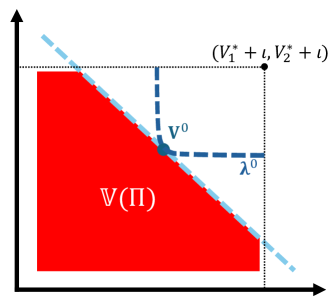
Figure 3: Illustration of Part 3)

Part 3) Prove that for a stochastic policy class $\Pi$, we have $\Pi_{\mathrm{W}}^{*}\subseteq\{\pi~{}|~{}\pi\in\mathop{\mathrm{argmin}}_{\pi\in\Pi}\mathrm{STCH}_{\bm{\lambda}}^{\mu}(\pi),\forall\bm{\lambda}\in\Delta_{m}\}$ and $\Pi_{\mathrm{P}}^{*}\subseteq\{\pi~{}|~{}\pi\in\mathop{\mathrm{argmin}}_{\pi\in\Pi}\mathrm{STCH}_{\bm{\lambda}}^{\mu}(\pi),\forall\bm{\lambda}\in\Delta_{m}^{o}\}$ for any $\mu>0$. According to Proposition 4.1, we know that $\mathbb{V}(\Pi)$ is a convex polytope when $\Pi$ is a stochastic policy class.

As shown in the Part 2) of the proof of Proposition 4.2, when $\mathbb{V}(\Pi)$ is a convex polytope, for any $\bm{V}^{0}$ on the Pareto front, one can find a hyperplane $\{\bm{V}\in\mathbb{R}^{m}|\sum_{i=1}^{m}a_{i}V_{i}=C\}$ with $a_{i}>0,C>0$ satisfying $\sum_{i=1}^{m}a_{i}V^{0}_{i}=C$ and $\mathbb{V}(\Pi)\subseteq\{\bm{V}\in\mathbb{R}^{m}|\sum_{i=1}^{m}a_{i}V_{i}\leq C\}$. With a slight abuse of notation, we view $\mathrm{STCH}_{\bm{\lambda}}^{\mu}$ as a function of $\bm{V}$ and denote $\mathrm{STCH}_{\bm{\lambda}}^{\mu}(\bm{V}):=\mu\log(\sum_{i=1}^{m}\exp(\lambda_{i}(V_{i}^{*}+\iota-V_{i})/\mu))$. For any $\mu>0$, if we can find positive $\lambda_{i}$’s such that $\bm{V}^{0}\in\mathop{\mathrm{argmin}}_{\bm{V}:\sum_{i=1}^{m}a_{i}V_{i}=C}\mathrm{STCH}_{\bm{\lambda}}^{\mu}(\bm{V})$, then

$$\min_{\bm{V}\in\mathbb{V}(\Pi)}\mathrm{STCH}_{\bm{\lambda}}^{\mu}(\bm{V})\leq\mathrm{STCH}_{\bm{\lambda}}^{\mu}(\bm{V}^{0}) =\min_{\bm{V}:\sum_{i=1}^{m}a_{i}V_{i}=C}\mathrm{STCH}_{\bm{\lambda}}^{\mu}(\bm{V})$$

$$=\min_{\bm{V}:\sum_{i=1}^{m}a_{i}V_{i}\leq C}\mathrm{STCH}_{\bm{\lambda}}^{\mu}(\bm{V})\leq\min_{\bm{V}\in\mathbb{V}(\Pi)}\mathrm{STCH}_{\bm{\lambda}}^{\mu}(\bm{V}),$$

which implies that $\bm{V}^{0}\in\mathop{\mathrm{argmin}}_{\bm{V}\in\mathbb{V}(\Pi)}\mathrm{STCH}_{\bm{\lambda}}^{\mu}(\bm{V}^{0})$. This leads to the desired result.

Consider the problem $\min_{\bm{V}:\sum_{i=1}^{m}a_{i}V_{i}=C}\mathrm{STCH}_{\bm{\lambda}}^{\mu}(\bm{V})$. It is equivalent to

$$\min_{\bm{V}:\sum_{i=1}^{m}a_{i}V_{i}=C}\sum_{i=1}^{m}\exp(\lambda_{i}(V_{i}^{*}+\iota-V_{i})/\mu),$$

since $\log$ is a strictly increasing function. The method of Lagrange multipliers leads to the conditions

$$\lambda_{i}\exp(\lambda_{i}(V_{i}^{*}+\iota-V_{i})/\mu)=\mu wa_{i},$$ (61)

where $w$ is the Lagrange multiplier. The LHS of (61) is an increasing function of $\lambda_{i}$ which goes to $0$ when $\lambda_{i}\to 0+$ and tends to $\infty$ when $\lambda_{i}\to\infty$. Therefore, for $w>0$, as $a_{i}>0$, we can always find $\lambda_{i}^{0}$’s such that $\lambda_{i}^{0}\exp(\lambda_{i}^{0}(V_{i}^{*}+\iota-V_{i}^{0})/\mu)=\mu wa_{i}$. Then, for $\bm{\lambda}^{0}=(\lambda_{1}^{0},\dots,\lambda_{m}^{0})$, we have $\bm{V}^{0}=\mathop{\mathrm{argmin}}_{\bm{V}\in\mathbb{V}(\Pi)}\mathrm{STCH}_{\bm{\lambda}^{0}}^{\mu}(\bm{V}^{0})$. One can adjust $w$ to make sure that $\sum_{i}\lambda_{i}^{0}=1$. The above construction is illustrated in Figure 3. This completes the proof for $\Pi_{\mathrm{P}}^{*}\subseteq\{\pi~{}|~{}\pi\in\mathop{\mathrm{argmin}}_{\pi\in\Pi}\mathrm{STCH}_{\bm{\lambda}}^{\mu}(\pi),\forall\bm{\lambda}\in\Delta_{m}^{o}\}$.

For any weak Pareto optimal policy, the only difference is that some $a_{i}$ might be 0. Set the corresponding $\lambda_{i}$ to be 0 completes the proof for $\Pi_{\mathrm{W}}^{*}\subseteq\{\pi~{}|~{}\pi\in\mathop{\mathrm{argmin}}_{\pi\in\Pi}\mathrm{STCH}_{\bm{\lambda}}^{\mu}(\pi),\forall\bm{\lambda}\in\Delta_{m}\}$.

Part 4) Now we use a concrete example to illustrate that for a deterministic policy class $\Pi$, a weakly Pareto optimal policy may not be the solution of $\min_{\pi\in\Pi}\mathrm{STCH}_{\bm{\lambda}}^{\mu}(\pi)$ for any $\bm{\lambda}\in\Delta_{m}$. We consider a multi-objective multi-arm bandit problem, a simple and special MOMDP whose state space size $|{\mathcal{S}}|=1$, episode length $H=1$, with a deterministic policy. Here we assume this bandit problem has $m=2$ reward functions $r_{1}$ and $r_{2}$ and $|\mathcal{A}|=3$ actions. We define

$$r_{1}(a_{1})=1,\quad r_{1}(a_{2})=0.5,\quad r_{1}(a_{3})=0.5,$$

$$r_{2}(a_{1})=0.5,\quad r_{2}(a_{2})=1,\quad r_{2}(a_{3})=0.5,$$

which are the reward values of the three actions for each reward function. Via the definition of the (weakly) Pareto optimal policy, we can find that $a_{1}$, $a_{2}$ are the Pareto optimal arms and that $a_{3}$ is a weakly Pareto optimal arm but not a Pareto optimal arm. Then, we have

$$\mathrm{STCH}_{\bm{\lambda}}^{\mu}(a_{1})=\mu\log(e^{\iota\lambda_{1}/\mu}+e^{(0.5+\iota)\lambda_{2}/\mu}),$$

$$\mathrm{STCH}_{\bm{\lambda}}^{\mu}(a_{2})=\mu\log(e^{(0.5+\iota)\lambda_{1}/\mu}+e^{\iota\lambda_{2}/\mu}),$$

$$\mathrm{STCH}_{\bm{\lambda}}^{\mu}(a_{3})=\mu\log(e^{(0.5+\iota)\lambda_{1}/\mu}+e^{(0.5+\iota)\lambda_{2}/\mu}),$$

which leads to (1) $\mathrm{STCH}_{\bm{\lambda}}^{\mu}(a_{3})>\mathrm{STCH}_{\bm{\lambda}}^{\mu}(a_{1})$ and $\mathrm{STCH}_{\bm{\lambda}}^{\mu}(a_{3})>\mathrm{STCH}_{\bm{\lambda}}^{\mu}(a_{2})$ when $\lambda_{1}>0$ and $\lambda_{2}>0$, (2) $\mathrm{STCH}_{\bm{\lambda}}^{\mu}(a_{3})>\mathrm{STCH}_{\bm{\lambda}}^{\mu}(a_{2})$ when $\lambda_{1}=0$ and $\lambda_{2}=1$, and (3) $\mathrm{STCH}_{\bm{\lambda}}^{\mu}(a_{3})>\mathrm{STCH}_{\bm{\lambda}}^{\mu}(a_{1})$ when $\lambda_{1}=1$ and $\lambda_{2}=0$. This implies that $a_{3}$ is not a minimizer of $\mathrm{STCH}_{\bm{\lambda}}^{\mu}(\pi)$ for any $\bm{\lambda}\in\Delta_{m}$ and $\mu>0$. The proof of this proposition is completed. ∎

E.2 Proof of Proposition 7.3

Proof.

According to Proposition 7.2, when $\lambda_{i}>0$, the solution to $\min_{\pi\in\Pi}\mathrm{STCH}_{\bm{\lambda}}^{\mu}(\pi)$ is Pareto optimal. We now prove that all Pareto optimal policies associated with the same $\bm{\lambda}$ have the same values on all objectives.

For the case where $\Pi$ is a stochastic policy class, assume that $\widetilde{\pi}$ and $\breve{\pi}$ are two solutions to $\min_{\pi\in\Pi}\mathrm{STCH}_{\bm{\lambda}}^{\mu}(\pi)$. Assume that there exists $i$ such that $V_{i,1}^{\widetilde{\pi}}(s_{1})\neq V_{i,1}^{\breve{\pi}}(s_{1})$. We let $\mathbb{V}(\Pi)$ be the set of $(V_{1,1}^{\pi}(s_{1}),\cdots,V_{m,1}^{\pi}(s_{1}))$ for all $\pi\in\Pi$. Then we have $\frac{1}{2}[(V_{1,1}^{\breve{\pi}}(s_{1}),\cdots,V_{m,1}^{\breve{\pi}}(s_{1}))+(V_{1,1}^{\widetilde{\pi}}(s_{1}),\cdots,V_{m,1}^{\widetilde{\pi}}(s_{1}))]\in\mathbb{V}(\Pi)$ since $\mathbb{V}(\Pi)$ is convex, which implies that there exists a policy $\pi^{\prime}$ such that

$$V_{i,1}^{\pi^{\prime}}(s_{1})=\frac{V_{1,1}^{\breve{\pi}}(s_{1})+V_{1,1}^{\widetilde{\pi}}(s_{1})}{2}.$$

On the other hand, the log-sum-exp function $\log\sum_{i=1}^{m}\exp x_{i}$ is strictly convex along any direction except for the direction of $(1,1,\cdots,1)$. We note that if $\left(\frac{\lambda_{1}(V_{1,1}^{*}(s_{1})+\tau-V_{1,1}^{\breve{\pi}}(s_{1}))}{\mu},\cdots,\frac{\lambda_{m}(V_{m,1}^{*}(s_{1})+\tau-V_{m,1}^{\breve{\pi}}(s_{1}))}{\mu}\right)\allowbreak-\left(\frac{\lambda_{1}(V_{1,1}^{*}(s_{1})+\tau-V_{1,1}^{\widetilde{\pi}}(s_{1}))}{\mu},\cdots,\frac{\lambda_{m}(V_{m,1}^{*}(s_{1})+\tau-V_{m,1}^{\widetilde{\pi}}(s_{1}))}{\mu}\right)=\alpha\cdot(1,1,\cdots,1)$ for some $\alpha\neq 0$, it contradicts that both $\breve{\pi}$ and $\widetilde{\pi}$ are Pareto optimal. Therefore, for policies $\widetilde{\pi}$ and $\breve{\pi}$ that do not satisfy the above condition, we can apply the strict convexity and obtain that

$$\mathrm{STCH}_{\bm{\lambda}}^{\mu}(\pi^{\prime})<\frac{\mathrm{STCH}_{\bm{\lambda}}^{\mu}(\breve{\pi})+\mathrm{STCH}_{\bm{\lambda}}^{\mu}(\widetilde{\pi})}{2}=\mathrm{STCH}_{\bm{\lambda}}^{\mu}(\breve{\pi}),$$

which additionally contradicts that $\breve{\pi}$ is a minimizer of $\mathrm{STCH}_{\bm{\lambda}}^{\mu}(\pi)$. Thus, we must have $V_{i,1}^{\widetilde{\pi}}(s_{1})=V_{i,1}^{\breve{\pi}}(s_{1})$ for any $i\in[m]$. This completes the first case.

If $\Pi$ is a deterministic policy class, for any $0<\mu<\mu^{*}$, the Pareto optimal policies that are the solutions to $\min_{\pi\in\Pi}\mathrm{STCH}_{\bm{\lambda}}^{\mu}(\pi)$ for all $\bm{\lambda}$ with $\lambda_{i}>0$ have the same values on all objectives.

Next, we prove this proposition for the deterministic policy class. Following the proof in Section E.1, when $\mu<\mu^{*}$, the optimal solution $\breve{\pi}$ to $\min_{\pi\in\Pi}\mathrm{STCH}_{\bm{\lambda}}^{\mu}(\pi)$ with $\lambda_{i}:=\frac{(V_{i,1}^{*}(s_{1})+\tau-V_{i,1}^{\breve{\pi}}(s_{1}))^{-1}}{\sum_{j=1}^{m}(V_{j,1}^{*}(s_{1})+\tau-V_{j,1}^{\breve{\pi}}(s_{1}))^{-1}}$ has the same values $V_{i,1}^{\breve{\pi}}(s_{1})$ for all $i\in[m]$ as any other optimal solutions to $\min_{\pi\in\Pi}\mathrm{STCH}_{\bm{\lambda}}^{\mu}(\pi)$. This completes the proof. ∎

E.3 Proof of Proposition 7.4

Proof.

The equivalent form in this proposition is obtained by applying the Fenchel conjugate of the log-sum-exp function [Boyd and Vandenberghe, 2004]. Then, we will consider to solve the following problem for any $\bm{\theta}\in\mathbb{R}^{m}$,

$$\max_{\bm{w}\in\Delta_{m}}\langle\bm{w},\bm{\theta}\rangle-\sum_{i=1}^{m}w_{i}\log w_{i}.$$ (62)

We note that $\langle\bm{w},\theta\rangle-\sum_{i=1}^{m}w_{i}\log w_{i}$ is a concave function. The Lagrangian function of the above problem is

$$L(\bm{w};\upsilon,\bm{\xi}):=\langle\bm{w},\theta\rangle-\sum_{i=1}^{m}w_{i}\log w_{i}+\upsilon\left(\sum_{i=1}^{m}w_{i}-1\right)+\sum_{i=1}^{m}\xi_{i}w_{i}.$$

Then, by KKT condition, we have

$$\frac{\partial L(\bm{w}^{*};\upsilon^{*},\bm{\xi}^{*})}{\partial w_{i}}=\theta_{i}-\log w_{i}^{*}-1+\upsilon^{*}+\xi_{i}^{*}=0,$$

$$\sum_{i=1}^{m}w_{i}^{*}-1=0,$$

$$\xi_{i}^{*}w_{i}^{*}=0,~{}~{}~{}\xi_{i}^{*}\geq 0,$$

where $(\bm{w}^{*},\upsilon^{*},\bm{x}^{*})$ is the solution to $\min_{\upsilon,\bm{\xi}}\max_{\bm{w}\in\Delta_{m}}L(\bm{w};\upsilon,\bm{\xi})$. By the first two equations above, we obtain that $w_{i}^{*}=\frac{\exp(\theta_{i}+\xi_{i}^{*})}{\sum_{i=1}^{m}\exp(\theta_{i}+\xi_{i}^{*})}>0$, which, combined with the third equation $\xi_{i}^{*}w_{i}^{*}=0$, further implies $\xi_{i}^{*}=0$ such that

$$w_{i}^{*}=\frac{\exp(\theta_{i})}{\sum_{i=1}^{m}\exp(\theta_{i})}.$$

Therefore, plugging $\bm{w}^{*}$ into (62), we have

$$\max_{\bm{w}\in\Delta_{m}}\langle\bm{w},\bm{\theta}\rangle-\sum_{i=1}^{m}w_{i}\log w_{i}=\log\left[\sum_{i=1}^{m}\exp(\theta_{i})\right].$$

Now we let $\theta_{i}=\frac{\lambda_{i}(V_{i,1}^{*}(s_{1})+\iota-V_{i,1}^{\pi}(s_{1}))}{\mu}$. Then, multiplying both sides of the above equation by $\mu$ yields

$$\mathrm{STCH}_{\bm{\lambda}}^{\mu}(\pi) =\mu\log\left[\sum_{i=1}^{m}\exp\left(\frac{\lambda_{i}(V_{i,1}^{*}(s_{1})+\iota-V_{i,1}^{\pi}(s_{1}))}{\mu}\right)\right]$$

$$=\max_{\bm{w}\in\Delta_{m}}\sum_{i=1}^{m}w_{i}\lambda_{i}(V_{i,1}^{*}(s_{1})+\iota-V_{i,1}^{\pi}(s_{1}))-\mu\sum_{i=1}^{m}w_{i}\log w_{i}.$$

Therefore, we eventually obtain that

$$\min_{\pi\in\Pi}\mathrm{STCH}_{\bm{\lambda}}^{\mu}(\pi)=\min_{\pi\in\Pi}\max_{\bm{w}\in\Delta_{m}}\max_{\nu_{i}\in\Pi}\sum_{i=1}^{m}w_{i}\lambda_{i}(V_{i,1}^{\nu_{i}}(s_{1})+\iota-V_{i,1}^{\pi}(s_{1}))-\mu\sum_{i=1}^{m}w_{i}\log w_{i}.$$

This completes the proof. ∎

E.4 Lemmas for Theorem 7.5 and Theorem 7.6

We note that the only differences between algorithms for Tchebycheff scalarization and algorithms for smooth Tchebycheff scalarization are the updating steps of $\bm{w}$. Therefore, to prove Theorem 7.5 and Theorem 7.6, we need to derive new lemmas for the updating steps of $\bm{w}$ in Algorithm 4 and Algorithm 5. We prove such lemmas in this section. Other lemmas for the proofs of Theorem 7.5 and Theorem 7.6 remain the same as the ones in Section C.2 and Section D.1.

Lemma E.1.

Setting $\eta_{t}=\frac{1}{\mu t}$ and $\alpha_{t}=\frac{1}{t^{2}}$ for $t\geq 1$, the updating rule of $\bm{w}$ in Algorithm 4 ensures

$$\max_{\bm{w}\in\Delta_{m}}\frac{1}{T}\sum_{t=1}^{T}\left[\langle\bm{w}-\bm{w}^{t},\bm{\lambda}\odot(\widetilde{\bm{V}}_{1}^{t}(s_{1})+\bm{\iota}-\bm{V}_{1}^{t}(s_{1}))\rangle-\mu\langle\bm{w},\log\bm{w}\rangle+\mu\langle\bm{w}^{t},\log\bm{w}^{t}\rangle\right]$$

$$\qquad\leq\frac{18H^{2}\log T}{\mu T}+\frac{11\mu\log^{3}(mT)}{T},$$

where we slightly abuse the logarithmic operator and let $\log\bm{w}:=[\log w_{1},\log w_{2},\cdots,\log w_{m}]$ be an element-wise logarithmic operation for the vector $\bm{w}$

Proof.

The mirror ascent step at the $(t+1)$-th episode is equivalent to solving the following minimization problem

$$\mathop{\mathrm{minimize}}_{\bm{w}\in\Delta_{m}}\quad -\eta_{t}\langle\bm{w},\bm{\lambda}\odot(\widetilde{\bm{V}}_{1}^{t}(s_{1})+\bm{\iota}-\bm{V}_{1}^{t}(s_{1}))-\mu\log\widetilde{\bm{w}}^{t}\rangle+D_{\mathrm{KL}}\big{(}\bm{w},\widetilde{\bm{w}}^{t}\big{)}.$$

We let $\bm{w}^{t+1}$ be the solution to the above optimization problem. Note that $\bm{w}^{t+1}$ is guaranteed to stay in the relative interior of a probability simplex if we initialize $w_{i}^{0}=1/m$. Thus, applying Lemma F.3 gives

$$\eta_{t}\langle\bm{w}-\bm{w}^{t+1},\bm{\lambda}\odot(\widetilde{\bm{V}}_{1}^{t}(s_{1})+\bm{\iota}-\bm{V}_{1}^{t}(s_{1}))-\mu\log\widetilde{\bm{w}}^{t}\rangle$$

$$\qquad\leq D_{\mathrm{KL}}\big{(}\bm{w},\widetilde{\bm{w}}^{t}\big{)}-D_{\mathrm{KL}}\big{(}\bm{w},\bm{w}^{t+1}\big{)}-D_{\mathrm{KL}}\big{(}\bm{w}^{t+1},\widetilde{\bm{w}}^{t}\big{)},$$

where $\bm{w}$ is an arbitrary variable in $\Delta_{m}$. Rearranging the terms leads to

$$\begin{aligned} &\eta_{t}\langle\bm{w}-\bm{w}^{t},\bm{\lambda}\odot(\widetilde{\bm{V}}_{1}^{t}(s_{1})+\bm{\iota}-\bm{V}_{1}^{t}(s_{1}))\rangle-\eta_{t}\mu\langle\bm{w},\log\bm{w}\rangle+\eta_{t}\mu\langle\bm{w}^{t},\log\bm{w}^{t}\rangle\\ &\qquad\leq D_{\mathrm{KL}}\big{(}\bm{w},\widetilde{\bm{w}}^{t}\big{)}-D_{\mathrm{KL}}\big{(}\bm{w},\bm{w}^{t+1}\big{)}-D_{\mathrm{KL}}\big{(}\bm{w}^{t+1},\widetilde{\bm{w}}^{t}\big{)}\\ &\qquad\quad+\eta_{t}\langle\bm{w}^{t+1}-\bm{w}^{t},\bm{\lambda}\odot(\widetilde{\bm{V}}_{1}^{t}(s_{1})+\bm{\iota}-\bm{V}_{1}^{t}(s_{1}))-\mu\log\widetilde{\bm{w}}^{t}\rangle\\ &\qquad\quad-\eta_{t}\mu\langle\bm{w},\log\bm{w}\rangle+\eta_{t}\mu\langle\bm{w}^{t},\log\bm{w}^{t}\rangle+\eta_{t}\mu\langle\bm{w}-\bm{w}^{t},\log\widetilde{\bm{w}}^{t}\rangle.\end{aligned}$$ (63)

For terms in RHS of (LABEL:eq:oco-11), by Lemma F.4 and the definition of KL divergence, we have

$$-D_{\mathrm{KL}}\big{(}\bm{w},\bm{w}^{t+1}\big{)}\leq-D_{\mathrm{KL}}\big{(}\bm{w},\widetilde{\bm{w}}^{t+1}\big{)}+\alpha_{t}\log m,$$

$$-\eta_{t}\mu\langle\bm{w},\log\bm{w}\rangle+\eta_{t}\mu\langle\bm{w}^{t},\log\bm{w}^{t}\rangle+\eta_{t}\mu\langle\bm{w}-\bm{w}^{t},\log\widetilde{\bm{w}}^{t}\rangle$$

$$\qquad=-\eta_{t}\mu D_{\mathrm{KL}}\big{(}\bm{w},\widetilde{\bm{w}}^{t}\big{)}+\eta_{t}\mu D_{\mathrm{KL}}\big{(}\bm{w}^{t},\widetilde{\bm{w}}^{t}\big{)}\leq-\eta_{t}\mu D_{\mathrm{KL}}\big{(}\bm{w},\widetilde{\bm{w}}^{t}\big{)}+\mu\eta_{t}\alpha_{t}\log m,$$

which thus leads to

$$\begin{aligned} &\eta_{t}\langle\bm{w}-\bm{w}^{t},\bm{\lambda}\odot(\widetilde{\bm{V}}_{1}^{t}(s_{1})+\bm{\iota}-\bm{V}_{1}^{t}(s_{1}))\rangle-\eta_{t}\mu\langle\bm{w},\log\bm{w}\rangle+\eta_{t}\mu\langle\bm{w}^{t},\log\bm{w}^{t}\rangle\\ &\qquad\leq(1-\eta_{t}\mu)D_{\mathrm{KL}}\big{(}\bm{w},\widetilde{\bm{w}}^{t}\big{)}-D_{\mathrm{KL}}\big{(}\bm{w},\widetilde{\bm{w}}^{t+1}\big{)}-D_{\mathrm{KL}}\big{(}\bm{w}^{t+1},\widetilde{\bm{w}}^{t}\big{)}+2\alpha_{t}\log m\\ &\qquad\quad+\eta_{t}\langle\bm{w}^{t+1}-\bm{w}^{t},\bm{\lambda}\odot(\widetilde{\bm{V}}_{1}^{t}(s_{1})+\bm{\iota}-\bm{V}_{1}^{t}(s_{1}))-\mu\log\widetilde{\bm{w}}^{t}\rangle,\end{aligned}$$ (64)

where we use the setting that $\mu\eta_{t}\leq 1$. In addition, by Pinsker’s inequality, we have

$$-D_{\mathrm{KL}}\big{(}\bm{w}^{t+1},\widetilde{\bm{w}}^{t}\big{)}\leq-\frac{1}{2}\big{\|}\bm{w}^{t+1}-\widetilde{\bm{w}}^{t}\big{\|}^{2}_{1}.$$

By Cauchy-Schwarz inequality, the last term in (LABEL:eq:oco-22) is bounded as

$$\eta_{t}\langle\bm{w}^{t+1}-\bm{w}^{t},\bm{\lambda}\odot(\widetilde{\bm{V}}_{1}^{t}(s_{1})+\bm{\iota}-\bm{V}_{1}^{t}(s_{1}))-\mu\log\widetilde{\bm{w}}^{t}\rangle$$

$$\qquad\leq\eta_{t}\|\bm{w}^{t+1}-\bm{w}^{t}\|_{1}\|\bm{\lambda}\odot(\widetilde{\bm{V}}_{1}^{t}(s_{1})+\bm{\iota}-\bm{V}_{1}^{t}(s_{1}))-\mu\log\widetilde{\bm{w}}^{t}\|_{\infty}$$

$$\qquad\leq\eta_{t}\left(\|\bm{w}^{t+1}-\widetilde{\bm{w}}^{t}\|_{1}+\|\widetilde{\bm{w}}^{t}-\bm{w}^{t}\|_{1}\right)\|\bm{\lambda}\odot(\widetilde{\bm{V}}_{1}^{t}(s_{1})+\bm{\iota}-\bm{V}_{1}^{t}(s_{1}))-\mu\log\widetilde{\bm{w}}^{t}\|_{\infty}$$

$$\qquad\leq\frac{1}{2}\big{\|}\bm{w}^{t+1}-\bm{w}^{t}\big{\|}_{1}^{2}+\left(3H+\mu\log(m/\alpha_{t})\right)^{2}\eta_{t}^{2}+2\alpha_{t}^{2},$$

where the last inequality uses Lemma F.4 and $\|\bm{\lambda}\odot(\widetilde{\bm{V}}_{1}^{t}(s_{1})+\bm{\iota}-\bm{V}_{1}^{t}(s_{1}))-\mu\log\widetilde{\bm{w}}^{t}\|_{\infty}=\max_{i}\lambda_{i}(\widetilde{V}_{i,1}^{t}(s_{1})+\iota-V_{i,1}^{t}(s_{1})))-\mu\log\widetilde{w}_{i}^{t}\leq 3H+\mu\log(m/\alpha_{t})$ with $\iota,\lambda_{i}\leq 1$. Plugging the above results in (LABEL:eq:oco-22), we have

$$\eta_{t}\langle\bm{w}-\bm{w}^{t},\bm{\lambda}\odot(\widetilde{\bm{V}}_{1}^{t}(s_{1})+\bm{\iota}-\bm{V}_{1}^{t}(s_{1}))\rangle-\eta_{t}\mu\langle\bm{w},\log\bm{w}\rangle+\eta_{t}\mu\langle\bm{w}^{t},\log\bm{w}^{t}\rangle$$

$$\qquad\leq(1-\eta_{t}\mu)D_{\mathrm{KL}}\big{(}\bm{w},\widetilde{\bm{w}}^{t}\big{)}-D_{\mathrm{KL}}\big{(}\bm{w},\widetilde{\bm{w}}^{t+1}\big{)}+2\alpha_{t}\log m+\left(3H+\mu\log(m/\alpha_{t})\right)^{2}\eta_{t}^{2}+2\alpha_{t}^{2},$$

Now setting $\eta_{t}=1/(\mu t)$ and $\alpha_{t}=1/t^{2}$, dividing both sides by $T\eta_{t}$, and taking summation from $1$ to $T$, we obtain

$$\frac{1}{T}\sum_{t=1}^{T}\left[\langle\bm{w}-\bm{w}^{t},\bm{\lambda}\odot(\widetilde{\bm{V}}_{1}^{t}(s_{1})+\bm{\iota}-\bm{V}_{1}^{t}(s_{1}))\rangle-\mu\langle\bm{w},\log\bm{w}\rangle+\mu\langle\bm{w}^{t},\log\bm{w}^{t}\rangle\right]$$

$$\qquad\leq\frac{1}{T}\sum_{t=1}^{T}\left[\mu(t-1)D_{\mathrm{KL}}\big{(}\bm{w},\widetilde{\bm{w}}^{t}\big{)}-\mu tD_{\mathrm{KL}}\big{(}\bm{w},\widetilde{\bm{w}}^{t+1}\big{)}+\frac{2\mu\log m}{t}+\frac{(3H+\mu\log(t^{2}m))^{2}}{\mu t}+\frac{2\mu}{t^{3}}\right]$$

$$\qquad\leq\frac{1}{T}\sum_{t=1}^{T}\left[\frac{2\mu\log m}{t}+\frac{(3H+2\mu\log(mt))^{2}}{\mu t}+\frac{2\mu}{t^{3}}\right]$$

$$\qquad\leq\frac{3\mu\log(mT)}{T}+\frac{(3H+2\mu\log(mT))^{2}\log T}{\mu T}\leq\frac{18H^{2}\log T}{\mu T}+\frac{11\mu\log^{3}(mT)}{T}.$$

This completes the proof. ∎

Lemma E.2.

Setting $\eta_{k}=\frac{1}{\mu k}$ and $\alpha_{k}=\frac{1}{k^{2}}$ for $k\geq 1$ and $\eta_{0}=\alpha_{0}=0$, the updating rule of $\bm{w}$ in Algorithm 5 ensures

$$\max_{\bm{w}\in\Delta_{m}}\frac{1}{K}\sum_{k=1}^{K}\left[\langle\bm{w}-\bm{w}^{k},\bm{\lambda}\odot(\widetilde{\bm{V}}_{1}(s_{1})+\bm{\iota}-\bm{V}_{1}^{k})\rangle-\mu\langle\bm{w},\log\bm{w}\rangle+\mu\langle\bm{w}^{k},\log\bm{w}^{k}\rangle\right]$$

$$\qquad\leq\frac{18H^{2}\log K}{\mu K}+\frac{11\mu\log^{3}(mK)}{K},$$

where we slightly abuse the logarithmic operator and let $\log\bm{w}:=[\log w_{1},\log w_{2},\cdots,\log w_{m}]$ be an element-wise logarithmic operation for the vector $\bm{w}$

Proof.

The proof of this lemma exactly follows the proof of Theorem E.1. ∎

E.5 Proof of Theorem 7.5

Proof.

We begin the proof of this theorem by decomposing $\mathrm{STCH}_{\bm{\lambda}}^{\mu}(\widehat{\pi})-\mathrm{STCH}_{\bm{\lambda}}^{\mu}(\pi_{\mu,\bm{\lambda}}^{*})$ where $\widehat{\pi}=\mathrm{Mix}(\pi^{1},\pi^{2},\cdots,\pi^{T})$. Specifically, following the decomposition analysis in Section C.3, we have

$$\begin{aligned} &\mathrm{STCH}_{\bm{\lambda}}^{\mu}(\widehat{\pi})-\mathrm{STCH}_{\bm{\lambda}}^{\mu}(\pi_{\mu,\bm{\lambda}}^{*})\\ &\qquad\leq\underbrace{\max_{\bm{w}\in\Delta_{m}}\frac{1}{T}\sum_{t=1}^{T}\sum_{i=1}^{m}w_{i}\lambda_{i}(V_{i,1}^{*}(s_{1})-V_{i,1}^{\widetilde{\nu}_{i}^{t}}(s_{1}))}_{\text{Term(I)}}\\ &\qquad\quad+\underbrace{\max_{\bm{w}\in\Delta_{m}}\frac{1}{T}\sum_{t=1}^{T}\sum_{i=1}^{m}[(w_{i}-w_{i}^{t})\lambda_{i}(V_{i,1}^{\widetilde{\nu}_{i}^{t}}(s_{1})+\iota-V_{i,1}^{\pi^{t}}(s_{1}))-w_{i}\log w_{i}+w_{i}^{t}\log w_{i}^{t}]}_{\text{Term(II)}}\\ &\qquad\quad+\underbrace{\frac{1}{T}\sum_{t=1}^{T}\sum_{i=1}^{m}w_{i}^{t}\lambda_{i}(V_{i,1}^{\pi_{\mu,\bm{\lambda}}^{*}}(s_{1})-V_{i,1}^{\pi^{t}}(s_{1}))}_{\text{Term(III)}}\end{aligned}$$ (65)

Then, we bound the above three terms respectively based on the updating rules in Algorithm 4. The only difference between Algorithm 1 for Tchebycheff scalarization and Algorithm 4 for smooth Tchebycheff scalarization are their updating steps of $\bm{w}$. As we can observe, only the upper bound of Term(II) corresponds to the updating step of $\bm{w}$. Thus, to prove Theorem 7.5, we can adopt the proof of Theorem 5.2 to provide the upper bounds of Term(I) and Term(III). Then, we have

$$\text{Term(I)}+\text{Term(III)}\leq\mathcal{O}\bigg{(}\sqrt{\frac{H^{4}|{\mathcal{S}}|^{2}|\mathcal{A}|\log(m|{\mathcal{S}}||\mathcal{A}|HT/\delta^{\prime})}{T}}\bigg{)},$$

with probability at least $1-\delta^{\prime}$. In addition, to bound Term(II), following the proof of Theorem 5.2, we further apply Lemma E.1 and obtain

Term(II) $$\leq\max_{\bm{w}\in\Delta_{m}}\frac{1}{T}\sum_{t=1}^{T}\left[\langle\bm{w}-\bm{w}^{t},\bm{\lambda}\odot(\widetilde{\bm{V}}_{1}^{t}(s_{1})+\bm{\iota}-\bm{V}_{1}^{t}(s_{1}))\rangle-\mu\langle\bm{w},\log\bm{w}\rangle+\mu\langle\bm{w}^{t},\log\bm{w}^{t}\rangle\right]$$

$$\quad+\frac{1}{T}\sum_{t=1}^{T}\sum_{i=1}^{m}\lambda_{i}(V_{i,1}^{t}(s_{1})-V_{i,1}^{\pi^{t}}(s_{1}))+\frac{1}{T}\sum_{t=1}^{T}\sum_{i=1}^{m}\lambda_{i}(\widetilde{V}_{i,1}^{t}(s_{1})-V_{i,1}^{\widetilde{\nu}_{i}^{t}}(s_{1}))$$

$$\leq\mathcal{O}\bigg{(}\sqrt{\frac{H^{4}|{\mathcal{S}}|^{2}|\mathcal{A}|\log(m|{\mathcal{S}}||\mathcal{A}|HT/\delta^{\prime})}{T}}\bigg{)}+\frac{18H^{2}\log T}{\mu T}+\frac{11\mu\log^{3}(mT)}{T}$$

with probability at least $1-\delta^{\prime}$. Further by (LABEL:eq:tch-decomp-11) and using the union bound, we obtain

$$\mathrm{STCH}_{\bm{\lambda}}^{\mu}(\widehat{\pi})-\mathrm{STCH}_{\bm{\lambda}}^{\mu}(\pi_{\mu,\bm{\lambda}}^{*})\leq\mathcal{O}\bigg{(}\sqrt{\frac{H^{4}|{\mathcal{S}}|^{2}|\mathcal{A}|\log(m|{\mathcal{S}}||\mathcal{A}|HT/\delta)}{T}}+\frac{H^{2}\log T}{\mu T}+\frac{\mu\log^{3}(mT)}{T}\bigg{)}$$

with probability at least $1-\delta$. This completes the proof of this theorem. ∎

E.6 Proof of Theorem 7.6

Proof.

We begin the proof of this theorem by decomposing $\mathrm{STCH}_{\bm{\lambda}}^{\mu}(\widehat{\pi})-\mathrm{STCH}_{\bm{\lambda}}^{\mu}(\pi_{\mu,\bm{\lambda}}^{*})$ where $\widehat{\pi}=\mathrm{Mix}(\pi^{1},\pi^{2},\cdots,\pi^{K})$. Specifically, following the decomposition analysis in Section D.2, we have

$$\begin{aligned} &\mathrm{STCH}_{\bm{\lambda}}^{\mu}(\widehat{\pi})-\mathrm{STCH}_{\bm{\lambda}}^{\mu}(\pi_{\mu,\bm{\lambda}}^{*})\\ &\qquad\leq\underbrace{\max_{\bm{w}\in\Delta_{m}}\frac{1}{T}\sum_{t=1}^{T}\sum_{i=1}^{m}w_{i}\lambda_{i}(V_{i,1}^{*}(s_{1})-V_{i,1}^{\widetilde{\nu}_{i}}(s_{1}))}_{\text{Term(I)}}\\ &\qquad\quad+\underbrace{\max_{\bm{w}\in\Delta_{m}}\frac{1}{T}\sum_{t=1}^{T}\sum_{i=1}^{m}[(w_{i}-w_{i}^{k})\lambda_{i}(V_{i,1}^{\widetilde{\nu}_{i}}(s_{1})+\iota-V_{i,1}^{\pi^{k}}(s_{1}))-w_{i}\log w_{i}+w_{i}^{k}\log w_{i}^{k}]}_{\text{Term(II)}}\\ &\qquad\quad+\underbrace{\frac{1}{T}\sum_{t=1}^{T}\sum_{i=1}^{m}w_{i}^{k}\lambda_{i}(V_{i,1}^{\pi_{\mu,\bm{\lambda}}^{*}}(s_{1})-V_{i,1}^{\pi^{k}}(s_{1}))}_{\text{Term(III)}}\end{aligned}$$ (66)

Then, we need to bound the above three terms respectively based on the updating rules in Algorithm 2 and Algorithm 5. The only difference between Algorithm 3 for Tchebycheff scalarization and Algorithm 5 for smooth Tchebycheff scalarization are their updating steps of $\bm{w}$. And only the upper bound of Term(II) corresponds to the updating step of $\bm{w}$. Thus, to prove Theorem 7.6, we can adapt the proof of Theorem 6.3 to provide the upper bounds of Term(I) and Term(III), which gives

$$\text{Term(I)}+\text{Term(III)}\leq\mathcal{O}\bigg{(}\sqrt{\frac{H^{6}|{\mathcal{S}}|^{2}|\mathcal{A}|\log(m|{\mathcal{S}}||\mathcal{A}|HT/\delta^{\prime})}{T}}\bigg{)},$$

with probability at least $1-\delta^{\prime}$ for option [I] in Algorithm 2, and

$$\text{Term(I)}+\text{Term(III)}\leq\mathcal{O}\bigg{(}\sqrt{\frac{(H^{2}|{\mathcal{S}}|+m)H^{4}|{\mathcal{S}}|^{2}|\mathcal{A}|\log(m|{\mathcal{S}}||\mathcal{A}|HT/\delta^{\prime})}{T}}\bigg{)},$$

with probability at least $1-\delta^{\prime}$ for option [II] in Algorithm 2.

In addition, to bound Term(II), following the proof of Theorem 6.3, we obtain

Term(II) $$\leq\max_{\bm{w}\in\Delta_{m}}\frac{1}{T}\sum_{t=1}^{T}\left[\langle\bm{w}-\bm{w}^{t},\bm{\lambda}\odot(\widetilde{\bm{V}}_{1}^{t}(s_{1})+\bm{\iota}-\bm{V}_{1}^{t}(s_{1}))\rangle-\mu\langle\bm{w},\log\bm{w}\rangle+\mu\langle\bm{w}^{t},\log\bm{w}^{t}\rangle\right]$$

$$\quad+\frac{1}{K}\sum_{k=1}^{K}\sum_{i=1}^{m}\lambda_{i}(V_{i,1}^{k}(s_{1})-V_{i,1}^{\pi^{k}}(s_{1}))+\sum_{i=1}^{m}\lambda_{i}(\widetilde{V}_{i,1}(s_{1})-V_{i,1}^{\widetilde{\nu}_{i}}(s_{1})).$$

Further applying Lemma E.2 leads to

$$\text{Term(II)}\leq\mathcal{O}\bigg{(}\sqrt{\frac{H^{6}|{\mathcal{S}}|^{2}|\mathcal{A}|\log(m|{\mathcal{S}}||\mathcal{A}|HT/\delta^{\prime})}{T}}\bigg{)}+\frac{18H^{2}\log K}{\mu K}+\frac{11\mu\log^{3}(mK)}{K}$$

with probability at least $1-\delta^{\prime}$ for option [I] in Algorithm 2, and

$$\text{Term(II)}\leq\mathcal{O}\bigg{(}\sqrt{\frac{(H^{2}|{\mathcal{S}}|+m)H^{4}|{\mathcal{S}}||\mathcal{A}|\log(m|{\mathcal{S}}||\mathcal{A}|HT/\delta^{\prime})}{T}}\bigg{)}+\frac{18H^{2}\log K}{\mu K}+\frac{11\mu\log^{3}(mK)}{K}$$

with probability at least $1-\delta^{\prime}$ option [II] in Algorithm 2. Combining the above results with (LABEL:eq:tch-decomp-22) and using the union bound, we obtain

$$\mathrm{STCH}_{\bm{\lambda}}^{\mu}(\widehat{\pi})-\mathrm{STCH}_{\bm{\lambda}}^{\mu}(\pi_{\mu,\bm{\lambda}}^{*})\leq\mathcal{O}\bigg{(}\sqrt{\frac{H^{6}|{\mathcal{S}}|^{2}|\mathcal{A}|\log(m|{\mathcal{S}}||\mathcal{A}|HT/\delta)}{T}}+\frac{H^{2}\log K}{\mu K}+\frac{\mu\log^{3}(mK)}{K}\bigg{)}$$

with probability at least $1-\delta$ for option [I], and

$$\mathrm{STCH}_{\bm{\lambda}}^{\mu}(\widehat{\pi})-\mathrm{STCH}_{\bm{\lambda}}^{\mu}(\pi_{\mu,\bm{\lambda}}^{*})\leq\mathcal{O}\bigg{(}\sqrt{\frac{(H^{2}|{\mathcal{S}}|+m)H^{4}|{\mathcal{S}}||\mathcal{A}|\log(m|{\mathcal{S}}||\mathcal{A}|HT/\delta)}{T}}+\frac{H^{2}\log K}{\mu K}+\frac{\mu\log^{3}(mK)}{K}\bigg{)}$$

with probability at least $1-\delta$ for option [II]. The proof of this theorem is completed. ∎

E.7 Additional Discussion for Algorithms

When $\mu$ is too small with $\mu\rightarrow 0^{+}$, we note that the results in Theorem 7.5 and Theorem 7.6 can be worse as they have a dependence on $1/\mu$. Here, we can further show that the term $\widetilde{\mathcal{O}}(1/(\mu T)+\mu/T)$ in Theorem 7.5 (or $\widetilde{\mathcal{O}}(1/(\mu K)+\mu/K)$ in Theorem 7.6) can be replaced by $\widetilde{\mathcal{O}}(1/\sqrt{T})$ (or $\widetilde{\mathcal{O}}(1/\sqrt{K})$) without the dependence on $1/\mu$ under different settings of the step size $\eta_{t}$ (or $\eta_{k}$).

Such results are associated with the learning guarantees for the update of $\bm{w}$, i.e., Lemmas E.1 and E.2. Next, We will derive the different guarantees under different step sizes for the update of $\bm{w}$ in Algorithm 4 and Algorithm 5. We remark that under this setting, the weighted average steps for $\bm{w}$ in both algorithms can be avoided. The proofs of the following lemmas will not use the weighted average steps, i.e., we substitute Line 3 and Line 4 in Algorithm 4 by

$$w_{i}^{t}\propto(w_{i}^{t-1})^{1-\mu\eta_{t-1}}\cdot\exp\{\eta_{t-1}\cdot\lambda_{i}(\widetilde{V}_{i,1}^{t-1}(s_{1})+\iota-V_{i,1}^{t-1}(s_{1}))\},~{}\forall i\in[m],$$ (67)

and substitute Line 8 and Line 9 in Algorithm 5 by

$$w_{i}^{k}\propto(w_{i}^{k-1})^{1-\mu\eta_{k-1}}\cdot\exp\{\eta_{k-1}\cdot\lambda_{i}(\widetilde{V}_{i,1}(s_{1})+\iota-V_{i,1}^{k-1}(s_{1}))\},~{}\forall i\in[m],$$ (68)

Lemma E.3.

When $\mu\leq 1$, Setting $\eta_{t}=\eta=1/(2H\sqrt{T})$, the updating rule of $\bm{w}$ in (67) for Algorithm 4 ensures

$$\max_{\bm{w}\in\Delta_{m}}\frac{1}{T}\sum_{t=1}^{T}\left[\langle\bm{w}-\bm{w}^{t},\bm{\lambda}\odot(\widetilde{\bm{V}}_{1}^{t}(s_{1})+\bm{\iota}-\bm{V}_{1}^{t}(s_{1}))\rangle-\mu\langle\bm{w},\log\bm{w}\rangle+\mu\langle\bm{w}^{t},\log\bm{w}^{t}\rangle\right]\leq\frac{2H\log m+5H}{\sqrt{T}}.$$

Proof.

The mirror ascent step at round $t+1$ via (67) is equivalent to solving the following minimization problem

$$\mathop{\mathrm{minimize}}_{\bm{w}\in\Delta_{m}}\quad -\eta_{t}\langle\bm{w},\bm{\lambda}\odot(\widetilde{\bm{V}}_{1}^{t}(s_{1})+\bm{\iota}-\bm{V}_{1}^{t}(s_{1}))-\mu\log\bm{w}^{t}\rangle+D_{\mathrm{KL}}\big{(}\bm{w},\bm{w}^{t}\big{)}.$$

Let $\bm{w}^{t+1}$ be the solution of the above optimization problem. Note that $\bm{w}^{t+1}$ is guaranteed to stay in the relative interior of a probability simplex if we initialize $w_{i}^{0}=1/m$. Thus, applying Lemma F.3 gives

$$-\eta_{t}\langle\bm{w}^{t+1},\bm{\lambda}\odot(\widetilde{\bm{V}}_{1}^{t}(s_{1})+\bm{\iota}-\bm{V}_{1}^{t}(s_{1}))-\mu\log\bm{w}^{t}\rangle+\eta_{t}\langle\bm{w},\bm{\lambda}\odot(\widetilde{\bm{V}}_{1}^{t}(s_{1})+\bm{\iota}-\bm{V}_{1}^{t}(s_{1}))-\mu\log\bm{w}^{t}\rangle$$

$$\qquad\leq D_{\mathrm{KL}}\big{(}\bm{w},\bm{w}^{t}\big{)}-D_{\mathrm{KL}}\big{(}\bm{w},\bm{w}^{t+1}\big{)}-D_{\mathrm{KL}}\big{(}\bm{w}^{t+1},\bm{w}^{t}\big{)},$$

where $\bm{w}$ is an arbitrary variable in $\Delta_{m}$. Rearranging the terms leads to

$$\begin{aligned} &\eta_{t}\langle\bm{w}-\bm{w}^{t},\bm{\lambda}\odot(\widetilde{\bm{V}}_{1}^{t}(s_{1})+\bm{\iota}-\bm{V}_{1}^{t}(s_{1}))\rangle-\eta_{t}\mu\langle\bm{w},\log\bm{w}\rangle+\eta_{t}\mu\langle\bm{w}^{t},\log\bm{w}^{t}\rangle\\ &\qquad\leq D_{\mathrm{KL}}\big{(}\bm{w},\bm{w}^{t}\big{)}-D_{\mathrm{KL}}\big{(}\bm{w},\bm{w}^{t+1}\big{)}-D_{\mathrm{KL}}\big{(}\bm{w}^{t+1},\bm{w}^{t}\big{)}\\ &\qquad\quad+\eta_{t}\langle\bm{w}^{t+1}-\bm{w}^{t},\bm{\lambda}\odot(\widetilde{\bm{V}}_{1}^{t}(s_{1})+\bm{\iota}-\bm{V}_{1}^{t}(s_{1}))\rangle\\ &\qquad\quad+\eta_{t}\mu\langle\bm{w}^{t}-\bm{w}^{t+1},\log\bm{w}^{t}\rangle+\eta_{t}\mu\langle\bm{w},\log\bm{w}^{t}-\log\bm{w}\rangle.\end{aligned}$$ (69)

We note that the last term of (LABEL:eq:oco-111) leads to $\eta_{t}\mu\langle\bm{w},\log\bm{w}^{t}-\log\bm{w}\rangle=-\eta_{t}\mu D_{\mathrm{KL}}(\bm{w},\bm{w}^{t})$ by the definition of KL divergence. Further by the definition of KL divergence, we have

$$\eta_{t}\mu\langle\bm{w}^{t}-\bm{w}^{t+1},\log\bm{w}^{t}\rangle=\eta_{t}\mu D_{\mathrm{KL}}(\bm{w}^{t+1},\bm{w}^{t})+\eta_{t}\mu\langle\bm{w}^{t},\log\bm{w}^{t}\rangle-\eta_{t}\mu\langle\bm{w}^{t+1},\log\bm{w}^{t+1}\rangle.$$

Therefore, (LABEL:eq:oco-111) is equivalently written as

$$\begin{aligned} &\eta_{t}\langle\bm{w}-\bm{w}^{t},\bm{\lambda}\odot(\widetilde{\bm{V}}_{1}^{t}(s_{1})+\bm{\iota}-\bm{V}_{1}^{t}(s_{1}))\rangle-\eta_{t}\mu\langle\bm{w},\log\bm{w}\rangle+\eta_{t}\mu\langle\bm{w}^{t},\log\bm{w}^{t}\rangle\\ &\qquad\leq(1-\eta_{t}\mu)D_{\mathrm{KL}}\big{(}\bm{w},\bm{w}^{t}\big{)}-D_{\mathrm{KL}}\big{(}\bm{w},\bm{w}^{t+1}\big{)}-(1-\eta_{t}\mu)D_{\mathrm{KL}}\big{(}\bm{w}^{t+1},\bm{w}^{t}\big{)}\\ &\qquad\quad+\eta_{t}\mu\langle\bm{w}^{t},\log\bm{w}^{t}\rangle-\eta_{t}\mu\langle\bm{w}^{t+1},\log\bm{w}^{t+1}\rangle\\ &\qquad\quad+\eta_{t}\langle\bm{w}^{t+1}-\bm{w}^{t},\bm{\lambda}\odot(\widetilde{\bm{V}}_{1}^{t}(s_{1})+\bm{\iota}-\bm{V}_{1}^{t}(s_{1}))\rangle.\end{aligned}$$ (70)

In addition, by Pinsker’s inequality, we have

$$-D_{\mathrm{KL}}\big{(}\bm{w}^{t+1},\bm{w}^{t}\big{)}\leq-\frac{1}{2}\big{\|}\bm{w}^{t+1}-\bm{w}^{t}\big{\|}^{2}_{1}.$$

By Cauchy-Schwarz inequality, the last term in (LABEL:eq:oco-222) is bounded as

$$\eta_{t}\langle\bm{w}^{t+1}-\bm{w}^{t},\bm{\lambda}\odot(\widetilde{\bm{V}}_{1}^{t}(s_{1})+\bm{\iota}-\bm{V}_{1}^{t}(s_{1}))\rangle$$

$$\qquad\leq\eta_{t}\|\bm{w}^{t+1}-\bm{w}^{t}\|_{1}\|\bm{\lambda}\odot(\widetilde{\bm{V}}_{1}^{t}(s_{1})+\bm{\iota}-\bm{V}_{1}^{t}(s_{1}))\|_{\infty}$$

$$\qquad\leq\frac{1-\eta_{t}\mu}{2}\big{\|}\bm{w}^{t+1}-\bm{w}^{t}\big{\|}_{1}^{2}+\frac{9H^{2}\eta_{t}^{2}}{2(1-\eta_{t}\mu)},$$

where the last inequality is due to $\|\bm{\lambda}\odot(\widetilde{\bm{V}}_{1}^{t}(s_{1})+\bm{\iota}-\bm{V}_{1}^{t}(s_{1}))\|_{\infty}^{2}=(\max_{i}\lambda_{i}(\widetilde{V}_{i,1}^{t}(s_{1})+\iota-V_{i,1}^{t}(s_{1})))^{2}\leq 9H^{2}$ with $\iota,\lambda_{i}\leq 1$. Therefore, combining the above inequalities with (LABEL:eq:oco-222), and due to $\eta_{t}\mu<1$, we have

$$\eta_{t}\langle\bm{w}-\bm{w}^{t},\bm{\lambda}\odot(\widetilde{\bm{V}}_{1}^{t}(s_{1})+\bm{\iota}-\bm{V}_{1}^{t}(s_{1}))\rangle-\eta_{t}\mu\langle\bm{w},\log\bm{w}\rangle+\eta_{t}\mu\langle\bm{w}^{t},\log\bm{w}^{t}\rangle$$

$$\qquad\leq(1-\eta_{t}\mu)D_{\mathrm{KL}}\big{(}\bm{w},\bm{w}^{t}\big{)}-D_{\mathrm{KL}}\big{(}\bm{w},\bm{w}^{t+1}\big{)}+\eta_{t}\mu\langle\bm{w}^{t},\log\bm{w}^{t}\rangle-\eta_{t}\mu\langle\bm{w}^{t+1},\log\bm{w}^{t+1}\rangle+\frac{9H^{2}\eta_{t}^{2}}{2(1-\eta_{t}\mu)}$$

$$\qquad\leq D_{\mathrm{KL}}\big{(}\bm{w},\bm{w}^{t}\big{)}-D_{\mathrm{KL}}\big{(}\bm{w},\bm{w}^{t+1}\big{)}+\eta_{t}\mu\langle\bm{w}^{t},\log\bm{w}^{t}\rangle-\eta_{t}\mu\langle\bm{w}^{t+1},\log\bm{w}^{t+1}\rangle+\frac{9H^{2}\eta_{t}^{2}}{2(1-\eta_{t}\mu)}.$$

Dividing both sides by $\eta_{t}$, setting $\eta_{t}=\eta$, and taking summation from $1$ to $T$ on both sides, we have

$$\sum_{t=1}^{T}\left[\langle\bm{w}-\bm{w}^{t},\bm{\lambda}\odot(\widetilde{\bm{V}}_{1}^{t}(s_{1})+\bm{\iota}-\bm{V}_{1}^{t}(s_{1}))\rangle-\mu\langle\bm{w},\log\bm{w}\rangle+\mu\langle\bm{w}^{t},\log\bm{w}^{t}\rangle\right]$$

$$\qquad\leq\sum_{t=1}^{T}\left(\frac{1}{\eta}D_{\mathrm{KL}}\big{(}\bm{w},\bm{w}^{t}\big{)}-\frac{1}{\eta}D_{\mathrm{KL}}\big{(}\bm{w},\bm{w}^{t+1}\big{)}\right)+5H^{2}\sum_{t=1}^{T}\frac{\eta}{1-\mu\eta}$$

$$\qquad\leq\frac{1}{\eta}D_{\mathrm{KL}}\big{(}\bm{w},\bm{w}^{1}\big{)}+5H^{2}\sum_{t=1}^{T}\frac{\eta}{1-\eta\mu}\leq\frac{\log m}{\eta}+5H^{2}\frac{T\eta}{1-\eta\mu}.$$

where the first inequality is due to the fact that our initialization of this algorithm ensures that $w_{i}^{1}=1/m$ such that $D_{\mathrm{KL}}\big{(}\bm{w},\bm{w}^{1}\big{)}=\sum_{i=1}^{m}w_{i}\log(w_{i}m)\leq\log m$. When $\mu\leq 1$, setting $\eta=1/(2H\sqrt{T})$, dividing both sides by $T$, we have

$$\max_{\bm{w}\in\Delta_{m}}\frac{1}{T}\sum_{t=1}^{T}(\bm{w}-\bm{w}^{t})^{\top}[\bm{\lambda}\odot(\widetilde{\bm{V}}_{1}^{t}(s_{1})+\bm{\iota}-\bm{V}_{1}^{t}(s_{1}))]\leq\frac{\log m}{T\eta}+10H^{2}\eta\leq\frac{2H\log m+5H}{\sqrt{T}},$$

where we use $1-\mu\eta\geq 1/2$. This completes the proof. ∎

Following the proof above, we similarly obtain the following lemma for Algorithm 5.

Lemma E.4.

When $\mu\leq 1$, setting $\eta_{k}=1/(2H\sqrt{T})$ for $k\geq 1$ and $0$ otherwise, the updating rule of $\bm{w}$ in (68) for Algorithm 5 ensures

$$\max_{\bm{w}\in\Delta_{m}}\frac{1}{K}\sum_{t=1}^{T}\left[\langle\bm{w}-\bm{w}^{k},\bm{\lambda}\odot(\widetilde{\bm{V}}_{1}(s_{1})+\bm{\iota}-\bm{V}_{1}^{k}(s_{1}))\rangle-\mu\langle\bm{w},\log\bm{w}\rangle+\mu\langle\bm{w}^{k},\log\bm{w}^{k}\rangle\right]\leq\frac{2H\log m+5H}{\sqrt{K}}.$$

Appendix F Other Supporting Lemmas

In the tabular case, once we collected $\ell$ trajectories, i.e., $\{s_{h}^{\tau},a_{h}^{\tau},r_{i,h}^{\tau}(s_{h}^{\tau},a_{h}^{\tau})\}_{\tau=1}^{\ell}$, we can always estimate the reward function and the transition kernel as

$$\widehat{r}_{i,h}(s,a)=\frac{\sum_{\tau=1}^{\ell}\mathbf{1}_{\{(s,a)=(s_{h}^{\tau},a_{h}^{\tau})\}}r_{i,h}^{\tau}(s_{h}^{\tau},a_{h}^{\tau})}{\max\{N_{h}(s,a),1\}},\quad\text{and}\quad\widehat{\mathbb{P}}_{h}(s^{\prime}|s,a)=\frac{N_{h}(s,a,s^{\prime})}{\max\{N_{h}(s,a),1\}},$$ (71)

where we define

$$N_{h}(s,a):=\sum_{\tau=1}^{\ell}\mathbf{1}_{\{(s,a)=(s_{h}^{\tau},a_{h}^{\tau})\}},\quad\text{and}\quad N_{h}(s,a,s^{\prime}):=\sum_{\tau=1}^{\ell}\mathbf{1}_{\{(s,a,s^{\prime})=(s_{h}^{\tau},a_{h}^{\tau},s_{h+1}^{\tau})\}}.$$

In what follows, we will show the estimation uncertainties based on the concentration inequalities, which correspond to the bonus terms that we are using in this work. The analysis of the concentration for the reward and transition estimation has been studied in many prior works on tabular MDPs (e.g., Strehl and Littman [2008], Jaksch et al. [2010], Azar et al. [2017], Qiu et al. [2020, 2021a]). For completeness, we present the proof in this section.

Lemma F.1.

Given a dataset $\{s_{h}^{\tau},a_{h}^{\tau},r_{i,h}^{\tau}(s_{h}^{\tau},a_{h}^{\tau})\}_{\tau=1}^{\ell}$ for an $\ell\geq 1$, for all $h\in[H]$ and all $(s,a)\in{\mathcal{S}}\times\mathcal{A}$, with probability at least $1-\delta$, we have

$$\big{|}\widehat{r}_{i,h}(s,a)-r_{i,h}(s,a)\big{|}\leq\sqrt{\frac{2\log(2|{\mathcal{S}}||\mathcal{A}|H/\delta)}{N_{h}(s,a)\vee 1}},$$

where $\widehat{r}_{i,h}(s,a)$ is defined as in (71), $r_{i,h}(s,a)$ is the true reward function, and $N_{h}(s,a):=\sum_{\tau=1}^{\ell}\mathbf{1}_{\{(s,a)=(s_{h}^{\tau},a_{h}^{\tau})\}}$.

Proof.

The proof for this lemma relies on an application of Hoeffding’s inequality. The definition of $\widehat{r}_{i,h}$ shows that $\widehat{r}_{i,h}(s,a)$ is the average of $N_{h}(s,a)$ samples of the observed rewards at $(s,a)$ when $N^{t-1}_{h}(s,a)>0$. Then, for fixed $\ell$, $h\in[H]$, and state-action tuple $(s,a)\in{\mathcal{S}}\times\mathcal{A}$, when $N^{t-1}_{h}(s,a)>0$, according to Hoeffding’s inequality, with probability at least $1-\delta^{\prime}$ where $\delta^{\prime}\in(0,1]$, we have

$$\big{|}\widehat{r}_{i,h}(s,a)-r_{i,h}(s,a)\big{|}\leq\sqrt{\frac{\log(2/\delta^{\prime})}{2N_{h}(s,a)}}.$$

When $N_{h}(s,a)=0$, we know $\widehat{r}_{i,h}(s,a)=0$ such that $|\widehat{r}_{i,h}(s,a)-r_{i,h}(s,a)|=|r_{i,h}(s,a)|\leq 1$. In addition, we have $\sqrt{2\log(2/\delta^{\prime})}\geq 1$. Combining the above results, with probability at least $1-\delta^{\prime}$, we have

$$\big{|}\widehat{r}_{i,h}(s,a)-r_{i,h}(s,a)\big{|}\leq\sqrt{\frac{2\log(2/\delta^{\prime})}{N_{h}(s,a)\vee 1}}.$$

Moreover, by the union bound, letting $\delta=|{\mathcal{S}}||\mathcal{A}|H\delta^{\prime}$, with probability at least $1-\delta$ where $\delta\in(0,1]$, for all $h\in[H]$ and all state-action tuple $(s,a)\in{\mathcal{S}}\times\mathcal{A}$, we have

$$\big{|}\widehat{r}_{i,h}(s,a)-r_{i,h}(s,a)\big{|}\leq\sqrt{\frac{2\log(2|{\mathcal{S}}||\mathcal{A}|H/\delta)}{\max\{N_{h}(s,a),1\}}}.$$

This completes the proof. ∎

Lemma F.2.

Given a dataset $\{s_{h}^{\tau},a_{h}^{\tau},r_{i,h}^{\tau}(s_{h}^{\tau},a_{h}^{\tau})\}_{\tau=1}^{\ell}$ for an $\ell>1$, for all $h\in[H]$ and all $(s,a)\in{\mathcal{S}}\times\mathcal{A}$, with probability at least $1-\delta$, we have

$$\left\|\widehat{\mathbb{P}}_{h}(\cdot{\,|\,}s,a)-\mathbb{P}_{h}(\cdot{\,|\,}s,a)\right\|_{1}\leq\sqrt{\frac{2|{\mathcal{S}}|\log(2|{\mathcal{S}}||\mathcal{A}|H/\delta)}{N_{h}(s,a)\vee 1}},$$

where $\widehat{\mathbb{P}}_{h}(s^{\prime}|s,a)$ is defined as in (71), $\mathbb{P}_{h}(s^{\prime}|s,a)$ is the true transition model, and $N_{h}(s,a):=\sum_{\tau=1}^{\ell}\mathbf{1}_{\{(s,a)=(s_{h}^{\tau},a_{h}^{\tau})\}}$.

Proof.

By the duality, we have $\|\widehat{\mathbb{P}}_{h}(\cdot{\,|\,}s,a)-\mathbb{P}_{h}(\cdot{\,|\,}s,a)\|_{1}=\sup_{\|\bm{z}\|_{\infty}\leq 1}~{}\langle\widehat{\mathbb{P}}_{h}(\cdot{\,|\,}s,a)-\mathbb{P}_{h}(\cdot{\,|\,}s,a),\bm{z}\rangle_{\mathcal{S}}$, where $\langle\cdot,\cdot\rangle_{\mathcal{S}}$ denotes the inner product over the state space ${\mathcal{S}}$. To bound this term, we construct an $\epsilon$-cover, denoted as $\mathcal{C}_{\infty}(\epsilon)$, for the set $\{\bm{z}\in\mathbb{R}^{|{\mathcal{S}}|}:\|\bm{z}\|_{\infty}\leq 1\}$ w.r.t. the $\ell_{\infty}$ distance such that for any $\bm{z}\in\mathbb{R}^{|{\mathcal{S}}|}$, there always exists $\bm{z}^{\prime}\in\mathcal{C}_{\infty}(\epsilon)$ satisfying $\|\bm{z}-\bm{z}^{\prime}\|_{\infty}\leq\epsilon$. The covering number is $\mathcal{N}_{\infty}(\epsilon)=|\mathcal{C}_{\infty}(\epsilon)|=1/\epsilon^{|{\mathcal{S}}|}$. Thus, we have for any $\bm{z}$ with $\|\bm{z}\|_{\infty}\leq 1$, there exists $\bm{z}^{\prime}\in\mathcal{C}_{\infty}(\epsilon)$ such that $\|\bm{z}^{\prime}-\bm{z}\|_{\infty}\leq\epsilon$ and

$$\big{\langle}\widehat{\mathbb{P}}_{h}(\cdot{\,|\,}s,a)-\mathbb{P}_{h}(\cdot{\,|\,}s,a),\bm{z}\big{\rangle}_{\mathcal{S}}$$

$$\qquad=\big{\langle}\widehat{\mathbb{P}}_{h}(\cdot{\,|\,}s,a)-\mathbb{P}_{h}(\cdot{\,|\,}s,a),\bm{z}^{\prime}\big{\rangle}_{\mathcal{S}}+\big{\langle}\widehat{\mathbb{P}}_{h}(\cdot{\,|\,}s,a)-\mathbb{P}_{h}(\cdot{\,|\,}s,a),\bm{z}-\bm{z}^{\prime}\big{\rangle}_{\mathcal{S}}$$

$$\qquad\leq\big{\langle}\widehat{\mathbb{P}}_{h}(\cdot{\,|\,}s,a)-\mathbb{P}_{h}(\cdot{\,|\,}s,a),\bm{z}^{\prime}\big{\rangle}_{\mathcal{S}}+\|\bm{z}-\bm{z}^{\prime}\|_{\infty}\left\|\widehat{\mathbb{P}}_{h}(\cdot{\,|\,}s,a)-\mathbb{P}_{h}(\cdot{\,|\,}s,a)\right\|_{1}$$

$$\qquad\leq\big{\langle}\widehat{\mathbb{P}}_{h}(\cdot{\,|\,}s,a)-\mathbb{P}_{h}(\cdot{\,|\,}s,a),\bm{z}^{\prime}\big{\rangle}_{\mathcal{S}}+\epsilon\left\|\widehat{\mathbb{P}}_{h}(\cdot{\,|\,}s,a)-\mathbb{P}_{h}(\cdot{\,|\,}s,a)\right\|_{1},$$

which leads to

$$\begin{aligned} &\left\|\widehat{\mathbb{P}}_{h}(\cdot{\,|\,}s,a)-\mathbb{P}_{h}(\cdot{\,|\,}s,a)\right\|_{1}\\ &\qquad=\sup_{\|\bm{z}\|_{\infty}\leq 1}~{}\big{\langle}\widehat{\mathbb{P}}_{h}(\cdot{\,|\,}s,a)-\mathbb{P}_{h}(\cdot{\,|\,}s,a),\bm{z}\big{\rangle}_{\mathcal{S}}\\ &\qquad\leq\sup_{\bm{z}^{\prime}\in\mathcal{C}_{\infty}(\epsilon)}~{}\big{\langle}\widehat{\mathbb{P}}_{h}(\cdot{\,|\,}s,a)-\mathbb{P}_{h}(\cdot{\,|\,}s,a),\bm{z}^{\prime}\big{\rangle}_{\mathcal{S}}+\epsilon\left\|\widehat{\mathbb{P}}_{h}(\cdot{\,|\,}s,a)-\mathbb{P}_{h}(\cdot{\,|\,}s,a)\right\|_{1}.\end{aligned}$$ (72)

By Hoeffding’s inequality and the union bound over all $\bm{z}^{\prime}\in\mathcal{C}_{\infty}(\epsilon)$, when $N_{h}(s,a)>0$, with probability at least $1-\delta^{\prime}$ where $\delta^{\prime}\in(0,1]$,

$$\max_{\bm{z}^{\prime}\in\mathcal{C}_{\infty}(\epsilon)}~{}\big{\langle}\widehat{\mathbb{P}}_{h}(\cdot{\,|\,}s,a)-\mathbb{P}_{h}(\cdot{\,|\,}s,a),\bm{z}^{\prime}\big{\rangle}_{\mathcal{S}}\leq\sqrt{\frac{|{\mathcal{S}}|\log(1/\epsilon)+\log(1/\delta^{\prime})}{2N_{h}(s,a)}}.$$ (73)

Letting $\epsilon=1/2$, by (LABEL:eq:net) and (73), with probability at least $1-\delta^{\prime}$, we have

$$\left\|\widehat{\mathbb{P}}_{h}(\cdot{\,|\,}s,a)-\mathbb{P}_{h}(\cdot{\,|\,}s,a)\right\|_{1}\leq 2\sqrt{\frac{|{\mathcal{S}}|\log 2+\log(1/\delta^{\prime})}{2N_{h}(s,a)}}.$$

When $N_{h}(s,a)=0$, we have $\big{\|}\widehat{\mathbb{P}}_{h}(\cdot{\,|\,}s,a)-\mathbb{P}_{h}(\cdot{\,|\,}s,a)\big{\|}_{1}=\|\mathbb{P}_{h}(\cdot{\,|\,}s,a)\|_{1}=1$. Moreover, $1<2\sqrt{\frac{|{\mathcal{S}}|\log 2+\log(1/\delta^{\prime})}{2}}$ holds. Thus, with probability at least $1-\delta^{\prime}$, we always have

$$\left\|\widehat{\mathbb{P}}_{h}(\cdot{\,|\,}s,a)-\mathbb{P}_{h}(\cdot{\,|\,}s,a)\right\|_{1}\leq 2\sqrt{\frac{|{\mathcal{S}}|\log 2+\log(1/\delta^{\prime})}{2\max\{N_{h}(s,a),1\}}}\leq\sqrt{\frac{2|{\mathcal{S}}|\log(2/\delta^{\prime})}{\max\{N_{h}(s,a),1\}}}.$$

Then, by the union bound, letting $\delta=|{\mathcal{S}}||\mathcal{A}|H\delta^{\prime}$, with probability at least $1-\delta$, for all $(s,a)\in{\mathcal{S}}\times\mathcal{A}$ and all $h\in[H]$, we have

$$\left\|\widehat{\mathbb{P}}_{h}(\cdot{\,|\,}s,a)-\mathbb{P}_{h}(\cdot{\,|\,}s,a)\right\|_{1}\leq\sqrt{\frac{2|{\mathcal{S}}|\log(2|{\mathcal{S}}||\mathcal{A}|H/\delta)}{\max\{N_{h}(s,a),1\}}},$$

which completes the proof. ∎

Next, we present a lemma that is commonly used in the proof of mirror descent algorithm.

Lemma F.3.

Let $f:\Delta_{n}\mapsto\mathbb{R}$ be a convex function, where $\Delta_{n}$ is the probability simplex in $\mathbb{R}^{n}$. For any $\alpha\geq 0$, $\bm{z}\in\Delta_{n}$, and $\bm{y}\in\Delta_{n}^{o}$ where $\Delta_{n}^{o}\subset\Delta_{n}$ is the relative interior of $\Delta_{n}^{o}$, supposing $\bm{x}^{\mathrm{opt}}=\mathop{\mathrm{argmin}}_{\bm{x}\in\Delta_{n}}f(\bm{x})+\beta D_{\mathrm{KL}}(\bm{x},\bm{y})$, then the following inequality holds

$$f(\bm{x}^{\mathrm{opt}})+\beta D_{\mathrm{KL}}(\bm{x}^{\mathrm{opt}},\bm{y})\leq f(\bm{z})+\beta D_{\mathrm{KL}}(\bm{z},\bm{y})-\beta D_{\mathrm{KL}}(\bm{z},\bm{x}^{\mathrm{opt}}),$$

where $D_{\mathrm{KL}}$ denotes the regular KL divergence, $D_{\mathrm{KL}}(\bm{x},\bm{y}):=\sum_{i=1}^{n}x_{i}\log\frac{x_{i}}{y_{i}}$.

This proof can be obtained by slight modification from prior works [Tseng, 2008, Nemirovski et al., 2009, Wei et al., 2019].

Next, we present a lemma that characterizes the difference between $\bm{x}\in\Delta_{n}$ and the vector $\widetilde{\bm{x}}\in\Delta_{n}$ that is a convex combination of $\bm{x}$ and an all-one vector.

Lemma F.4 (Wei et al. [2019], Qiu et al. [2023]).

Suppose that $\bm{x}\in\Delta_{n}$ and $\widetilde{x}_{i}=(1-\alpha)x_{i}+\alpha/n$

$$D_{\mathrm{KL}}(\bm{y},\widetilde{\bm{x}})-D_{\mathrm{KL}}(\bm{y},\bm{x})\leq\alpha\log n,~{}~{}\forall\bm{y}\in\Delta_{n},$$

$$\|\widetilde{\bm{x}}-\bm{x}\|_{1}\leq 2\alpha,$$

where $D_{\mathrm{KL}}$ denotes the regular KL divergence.

References

• Agarwal et al. (2022) M. Agarwal, V. Aggarwal, and T. Lan. Multi-objective reinforcement learning with non-linear scalarization. In Proceedings of the 21st International Conference on Autonomous Agents and Multiagent Systems, pages 9–17, 2022.
• Altman (2021) E. Altman. Constrained Markov decision processes. Routledge, 2021.
• Andrychowicz et al. (2017) M. Andrychowicz, F. Wolski, A. Ray, J. Schneider, R. Fong, P. Welinder, B. McGrew, J. Tobin, O. Pieter Abbeel, and W. Zaremba. Hindsight experience replay. Advances in neural information processing systems, 30, 2017.
• Azar et al. (2017) M. G. Azar, I. Osband, and R. Munos. Minimax regret bounds for reinforcement learning. In International conference on machine learning, pages 263–272. PMLR, 2017.
• Barrett and Narayanan (2008) L. Barrett and S. Narayanan. Learning all optimal policies with multiple criteria. In Proceedings of the 25th international conference on Machine learning, pages 41–47, 2008.
• Beck and Teboulle (2012) A. Beck and M. Teboulle. Smoothing and first order methods: A unified framework. SIAM Journal on Optimization, 22(2):557–580, 2012.
• Bowman Jr (1976) V. J. Bowman Jr. On the relationship of the tchebycheff norm and the efficient frontier of multiple-criteria objectives. In Multiple Criteria Decision Making: Proceedings of a Conference Jouy-en-Josas, France May 21–23, 1975, pages 76–86. Springer, 1976.
• Boyd and Vandenberghe (2004) S. P. Boyd and L. Vandenberghe. Convex optimization. Cambridge university press, 2004.
• Busa-Fekete et al. (2017) R. Busa-Fekete, B. Szörényi, P. Weng, and S. Mannor. Multi-objective bandits: Optimizing the generalized gini index. In International Conference on Machine Learning, pages 625–634. PMLR, 2017.
• Caramia et al. (2020) M. Caramia, P. Dell’Olmo, M. Caramia, and P. Dell’Olmo. Multi-objective optimization. Multi-objective Management in Freight Logistics: Increasing Capacity, Service Level, Sustainability, and Safety with Optimization Algorithms, pages 21–51, 2020.
• Chen et al. (2022) J. Chen, A. Modi, A. Krishnamurthy, N. Jiang, and A. Agarwal. On the statistical efficiency of reward-free exploration in non-linear rl. Advances in Neural Information Processing Systems, 35:20960–20973, 2022.
• Chen et al. (2024) L. Chen, H. Fernando, Y. Ying, and T. Chen. Three-way trade-off in multi-objective learning: Optimization, generalization and conflict-avoidance. Advances in Neural Information Processing Systems, 36, 2024.
• Chen et al. (2023) W. Chen, J. Tian, C. Fan, Y. Li, H. He, and Y. Jin. Preference-controlled multi-objective reinforcement learning for conditional text generation. In Proceedings of the AAAI Conference on Artificial Intelligence, volume 37, pages 12662–12672, 2023.
• Chen (2012) X. Chen. Smoothing methods for nonsmooth, nonconvex minimization. Mathematical programming, 134:71–99, 2012.
• Chen et al. (2019) X. Chen, A. Ghadirzadeh, M. Björkman, and P. Jensfelt. Meta-learning for multi-objective reinforcement learning. In 2019 IEEE/RSJ International Conference on Intelligent Robots and Systems (IROS), pages 977–983. IEEE, 2019.
• Chen et al. (2020) Z. Chen, J. Ngiam, Y. Huang, T. Luong, H. Kretzschmar, Y. Chai, and D. Anguelov. Just pick a sign: Optimizing deep multitask models with gradient sign dropout. Advances in Neural Information Processing Systems, 33:2039–2050, 2020.
• Cheng et al. (2023) Y. Cheng, R. Huang, J. Yang, and Y. Liang. Improved sample complexity for reward-free reinforcement learning under low-rank mdps. arXiv preprint arXiv:2303.10859, 2023.
• Choo and Atkins (1983) E. U. Choo and D. R. Atkins. Proper efficiency in nonconvex multicriteria programming. Mathematics of Operations Research, 8(3):467–470, 1983.
• Das and Dennis (1997) I. Das and J. E. Dennis. A closer look at drawbacks of minimizing weighted sums of objectives for pareto set generation in multicriteria optimization problems. Structural optimization, 14:63–69, 1997.
• Deb et al. (2016) K. Deb, K. Sindhya, and J. Hakanen. Multi-objective optimization. In Decision sciences, pages 161–200. CRC Press, 2016.
• Drugan and Nowe (2013) M. M. Drugan and A. Nowe. Designing multi-objective multi-armed bandits algorithms: A study. In The 2013 international joint conference on neural networks (IJCNN), pages 1–8. IEEE, 2013.
• Ehrgott (2005) M. Ehrgott. Multicriteria optimization, volume 491. Springer Science & Business Media, 2005.
• Ehrgott and Wiecek (2005) M. Ehrgott and M. M. Wiecek. Multiobjective programming. Multiple criteria decision analysis: State of the art surveys, 78:667–708, 2005.
• Fernando et al. (2022) H. D. Fernando, H. Shen, M. Liu, S. Chaudhury, K. Murugesan, and T. Chen. Mitigating gradient bias in multi-objective learning: A provably convergent approach. In The Eleventh International Conference on Learning Representations, 2022.
• Geoffrion (1968) A. M. Geoffrion. Proper efficiency and the theory of vector maximization. Journal of mathematical analysis and applications, 22(3):618–630, 1968.
• Giagkiozis and Fleming (2015) I. Giagkiozis and P. J. Fleming. Methods for multi-objective optimization: An analysis. Information Sciences, 293:338–350, 2015.
• Gunantara (2018) N. Gunantara. A review of multi-objective optimization: Methods and its applications. Cogent Engineering, 5(1):1502242, 2018.
• Guo et al. (2024) Y. Guo, G. Cui, L. Yuan, N. Ding, J. Wang, H. Chen, B. Sun, R. Xie, J. Zhou, Y. Lin, et al. Controllable preference optimization: Toward controllable multi-objective alignment. arXiv preprint arXiv:2402.19085, 2024.
• Hayes et al. (2022) C. F. Hayes, R. Rădulescu, E. Bargiacchi, J. Källström, M. Macfarlane, M. Reymond, T. Verstraeten, L. M. Zintgraf, R. Dazeley, F. Heintz, et al. A practical guide to multi-objective reinforcement learning and planning. Autonomous Agents and Multi-Agent Systems, 36(1):26, 2022.
• Hu et al. (2024) Y. Hu, R. Xian, Q. Wu, Q. Fan, L. Yin, and H. Zhao. Revisiting scalarization in multi-task learning: A theoretical perspective. Advances in Neural Information Processing Systems, 36, 2024.
• Hwang et al. (2023) M. Hwang, L. Weihs, C. Park, K. Lee, A. Kembhavi, and K. Ehsani. Promptable behaviors: Personalizing multi-objective rewards from human preferences. arXiv preprint arXiv:2312.09337, 2023.
• Jaksch et al. (2010) T. Jaksch, R. Ortner, and P. Auer. Near-optimal regret bounds for reinforcement learning. Journal of Machine Learning Research, 11:1563–1600, 2010.
• Jiang et al. (2023) J. Jiang, W. Zhang, S. Zhou, L. Gu, X. Zeng, and W. Zhu. Multi-objective online learning. In The Eleventh International Conference on Learning Representations, 2023. URL https://openreview.net/forum?id=dKkMnCWfVmm.
• Jin et al. (2020a) C. Jin, A. Krishnamurthy, M. Simchowitz, and T. Yu. Reward-free exploration for reinforcement learning. In International Conference on Machine Learning, pages 4870–4879. PMLR, 2020a.
• Jin et al. (2020b) C. Jin, Z. Yang, Z. Wang, and M. I. Jordan. Provably efficient reinforcement learning with linear function approximation. In Conference on learning theory, pages 2137–2143. PMLR, 2020b.
• Kasimbeyli et al. (2019) R. Kasimbeyli, Z. K. Ozturk, N. Kasimbeyli, G. D. Yalcin, and B. I. Erdem. Comparison of some scalarization methods in multiobjective optimization: comparison of scalarization methods. Bulletin of the Malaysian Mathematical Sciences Society, 42:1875–1905, 2019.
• Klamroth and Jørgen (2007) K. Klamroth and T. Jørgen. Constrained optimization using multiple objective programming. Journal of Global Optimization, 37:325–355, 2007.
• Li et al. (2020) K. Li, T. Zhang, and R. Wang. Deep reinforcement learning for multiobjective optimization. IEEE transactions on cybernetics, 51(6):3103–3114, 2020.
• Lin et al. (2024) X. Lin, X. Zhang, Z. Yang, F. Liu, Z. Wang, and Q. Zhang. Smooth tchebycheff scalarization for multi-objective optimization. arXiv preprint arXiv:2402.19078, 2024.
• Liu et al. (2021a) B. Liu, X. Liu, X. Jin, P. Stone, and Q. Liu. Conflict-averse gradient descent for multi-task learning. Advances in Neural Information Processing Systems, 34:18878–18890, 2021a.
• Liu et al. (2021b) X. Liu, X. Tong, and Q. Liu. Profiling Pareto front with multi-objective stein variational gradient descent. Advances in Neural Information Processing Systems, 34:14721–14733, 2021b.
• Lu et al. (2022) H. Lu, D. Herman, and Y. Yu. Multi-objective reinforcement learning: Convexity, stationarity and pareto optimality. In The Eleventh International Conference on Learning Representations, 2022.
• Lu et al. (2019) S. Lu, G. Wang, Y. Hu, and L. Zhang. Multi-objective generalized linear bandits. arXiv preprint arXiv:1905.12879, 2019.
• Mahapatra and Rajan (2020) D. Mahapatra and V. Rajan. Multi-task learning with user preferences: Gradient descent with controlled ascent in Pareto optimization. In International Conference on Machine Learning, pages 6597–6607. PMLR, 2020.
• Mahapatra et al. (2023) D. Mahapatra, C. Dong, Y. Chen, and M. Momma. Multi-label learning to rank through multi-objective optimization. In Proceedings of the 29th ACM SIGKDD Conference on Knowledge Discovery and Data Mining, pages 4605–4616, 2023.
• Miettinen (1999) K. Miettinen. Nonlinear multiobjective optimization, volume 12. Springer Science & Business Media, 1999.
• Miryoosefi and Jin (2022) S. Miryoosefi and C. Jin. A simple reward-free approach to constrained reinforcement learning. In International Conference on Machine Learning, pages 15666–15698. PMLR, 2022.
• Modi et al. (2024) A. Modi, J. Chen, A. Krishnamurthy, N. Jiang, and A. Agarwal. Model-free representation learning and exploration in low-rank mdps. Journal of Machine Learning Research, 25(6):1–76, 2024.
• Natarajan and Tadepalli (2005) S. Natarajan and P. Tadepalli. Dynamic preferences in multi-criteria reinforcement learning. In Proceedings of the 22nd international conference on Machine learning, pages 601–608, 2005.
• Nemirovski et al. (2009) A. Nemirovski, A. Juditsky, G. Lan, and A. Shapiro. Robust stochastic approximation approach to stochastic programming. SIAM Journal on optimization, 19(4):1574–1609, 2009.
• Nesterov (2005) Y. Nesterov. Smooth minimization of non-smooth functions. Mathematical programming, 103:127–152, 2005.
• Perez et al. (2010) J. Perez, C. Germain-Renaud, B. Kégl, and C. Loomis. Multi-objective reinforcement learning for responsive grids. Journal of Grid Computing, 8:473–492, 2010.
• Pirotta et al. (2015) M. Pirotta, S. Parisi, and M. Restelli. Multi-objective reinforcement learning with continuous pareto frontier approximation. In Proceedings of the AAAI conference on artificial intelligence, volume 29, 2015.
• Puterman (1990) M. L. Puterman. Markov decision processes. Handbooks in operations research and management science, 2:331–434, 1990.
• Qiao and Wang (2022) D. Qiao and Y.-X. Wang. Near-optimal deployment efficiency in reward-free reinforcement learning with linear function approximation. arXiv preprint arXiv:2210.00701, 2022.
• Qiu et al. (2020) S. Qiu, X. Wei, Z. Yang, J. Ye, and Z. Wang. Upper confidence primal-dual reinforcement learning for cmdp with adversarial loss. Advances in Neural Information Processing Systems, 33:15277–15287, 2020.
• Qiu et al. (2021a) S. Qiu, X. Wei, J. Ye, Z. Wang, and Z. Yang. Provably efficient fictitious play policy optimization for zero-sum markov games with structured transitions. In International Conference on Machine Learning, pages 8715–8725. PMLR, 2021a.
• Qiu et al. (2021b) S. Qiu, J. Ye, Z. Wang, and Z. Yang. On reward-free rl with kernel and neural function approximations: Single-agent mdp and markov game. In International Conference on Machine Learning, pages 8737–8747. PMLR, 2021b.
• Qiu et al. (2023) S. Qiu, X. Wei, and M. Kolar. Gradient-variation bound for online convex optimization with constraints. In Proceedings of the AAAI Conference on Artificial Intelligence, volume 37, pages 9534–9542, 2023.
• Riquelme et al. (2015) N. Riquelme, C. Von Lücken, and B. Baran. Performance metrics in multi-objective optimization. In 2015 Latin American computing conference (CLEI), pages 1–11. IEEE, 2015.
• Roijers et al. (2013) D. M. Roijers, P. Vamplew, S. Whiteson, and R. Dazeley. A survey of multi-objective sequential decision-making. Journal of Artificial Intelligence Research, 48:67–113, 2013.
• Sener and Koltun (2018) O. Sener and V. Koltun. Multi-task learning as multi-objective optimization. Advances in neural information processing systems, 31, 2018.
• Stamenkovic et al. (2022) D. Stamenkovic, A. Karatzoglou, I. Arapakis, X. Xin, and K. Katevas. Choosing the best of both worlds: Diverse and novel recommendations through multi-objective reinforcement learning. In Proceedings of the Fifteenth ACM International Conference on Web Search and Data Mining, pages 957–965, 2022.
• Steuer (1986) R. E. Steuer. Multiple criteria optimization. Theory, computation, and application, 1986.
• Strehl and Littman (2008) A. L. Strehl and M. L. Littman. An analysis of model-based interval estimation for markov decision processes. Journal of Computer and System Sciences, 74(8):1309–1331, 2008.
• Tekin and Turğay (2018) C. Tekin and E. Turğay. Multi-objective contextual multi-armed bandit with a dominant objective. IEEE Transactions on Signal Processing, 66(14):3799–3813, 2018.
• Tseng (2008) P. Tseng. On accelerated proximal gradient methods for convex-concave optimization. submitted to SIAM Journal on Optimization, 1, 2008.
• Turgay et al. (2018) E. Turgay, D. Oner, and C. Tekin. Multi-objective contextual bandit problem with similarity information. In International Conference on Artificial Intelligence and Statistics, pages 1673–1681. PMLR, 2018.
• v. Neumann (1928) J. v. Neumann. Zur theorie der gesellschaftsspiele. Mathematische annalen, 100(1):295–320, 1928.
• Van Moffaert and Nowé (2014) K. Van Moffaert and A. Nowé. Multi-objective reinforcement learning using sets of pareto dominating policies. The Journal of Machine Learning Research, 15(1):3483–3512, 2014.
• Van Moffaert et al. (2013a) K. Van Moffaert, M. M. Drugan, and A. Nowé. Hypervolume-based multi-objective reinforcement learning. In Evolutionary Multi-Criterion Optimization: 7th International Conference, EMO 2013, Sheffield, UK, March 19-22, 2013. Proceedings 7, pages 352–366. Springer, 2013a.
• Van Moffaert et al. (2013b) K. Van Moffaert, M. M. Drugan, and A. Nowé. Scalarized multi-objective reinforcement learning: Novel design techniques. In 2013 IEEE symposium on adaptive dynamic programming and reinforcement learning (ADPRL), pages 191–199. IEEE, 2013b.
• Wang et al. (2024) H. Wang, Y. Lin, W. Xiong, R. Yang, S. Diao, S. Qiu, H. Zhao, and T. Zhang. Arithmetic control of llms for diverse user preferences: Directional preference alignment with multi-objective rewards. arXiv preprint arXiv:2402.18571, 2024.
• Wang et al. (2020) R. Wang, S. S. Du, L. Yang, and R. R. Salakhutdinov. On reward-free reinforcement learning with linear function approximation. Advances in neural information processing systems, 33:17816–17826, 2020.
• Wang and Sebag (2013) W. Wang and M. Sebag. Hypervolume indicator and dominance reward based multi-objective monte-carlo tree search. Machine learning, 92:403–429, 2013.
• Wei et al. (2019) X. Wei, H. Yu, and M. J. Neely. Online primal-dual mirror descent under stochastic constraints. arXiv preprint arXiv:1908.00305, 2019.
• Wiering et al. (2014) M. A. Wiering, M. Withagen, and M. M. Drugan. Model-based multi-objective reinforcement learning. In 2014 IEEE symposium on adaptive dynamic programming and reinforcement learning (ADPRL), pages 1–6. IEEE, 2014.
• Wu et al. (2021a) J. Wu, V. Braverman, and L. Yang. Accommodating picky customers: Regret bound and exploration complexity for multi-objective reinforcement learning. Advances in Neural Information Processing Systems, 34:13112–13124, 2021a.
• Wu et al. (2021b) R. Wu, Y. Zhang, Z. Yang, and Z. Wang. Offline constrained multi-objective reinforcement learning via pessimistic dual value iteration. Advances in Neural Information Processing Systems, 34:25439–25451, 2021b.
• Xiao et al. (2024) P. Xiao, H. Ban, and K. Ji. Direction-oriented multi-objective learning: Simple and provable stochastic algorithms. Advances in Neural Information Processing Systems, 36, 2024.
• Xu et al. (2020) J. Xu, Y. Tian, P. Ma, D. Rus, S. Sueda, and W. Matusik. Prediction-guided multi-objective reinforcement learning for continuous robot control. In International conference on machine learning, pages 10607–10616. PMLR, 2020.
• Yahyaa et al. (2014a) S. Q. Yahyaa, M. M. Drugan, and B. Manderick. Annealing-pareto multi-objective multi-armed bandit algorithm. In 2014 IEEE Symposium on Adaptive Dynamic Programming and Reinforcement Learning (ADPRL), pages 1–8. IEEE, 2014a.
• Yahyaa et al. (2014b) S. Q. Yahyaa, M. M. Drugan, and B. Manderick. The scalarized multi-objective multi-armed bandit problem: An empirical study of its exploration vs. exploitation tradeoff. In 2014 International Joint Conference on Neural Networks (IJCNN), pages 2290–2297. IEEE, 2014b.
• Yala et al. (2022) A. Yala, P. G. Mikhael, C. Lehman, G. Lin, F. Strand, Y.-L. Wan, K. Hughes, S. Satuluru, T. Kim, I. Banerjee, et al. Optimizing risk-based breast cancer screening policies with reinforcement learning. Nature medicine, 28(1):136–143, 2022.
• Yang et al. (2019) R. Yang, X. Sun, and K. Narasimhan. A generalized algorithm for multi-objective reinforcement learning and policy adaptation. Advances in neural information processing systems, 32, 2019.
• Yang et al. (2024) R. Yang, X. Pan, F. Luo, S. Qiu, H. Zhong, D. Yu, and J. Chen. Rewards-in-context: Multi-objective alignment of foundation models with dynamic preference adjustment. arXiv preprint arXiv:2402.10207, 2024.
• Yang et al. (2020) Z. Yang, C. Jin, Z. Wang, M. Wang, and M. Jordan. Provably efficient reinforcement learning with kernel and neural function approximations. Advances in Neural Information Processing Systems, 33:13903–13916, 2020.
• Yu et al. (2021a) T. Yu, A. Kumar, Y. Chebotar, K. Hausman, S. Levine, and C. Finn. Conservative data sharing for multi-task offline reinforcement learning. Advances in Neural Information Processing Systems, 34:11501–11516, 2021a.
• Yu et al. (2021b) T. Yu, Y. Tian, J. Zhang, and S. Sra. Provably efficient algorithms for multi-objective competitive RL. In International Conference on Machine Learning, pages 12167–12176. PMLR, 2021b.
• Zhang et al. (2023) J. Zhang, W. Zhang, and Q. Gu. Optimal horizon-free reward-free exploration for linear mixture mdps. In International Conference on Machine Learning, pages 41902–41930. PMLR, 2023.
• Zhang et al. (2021) Z. Zhang, S. Du, and X. Ji. Near optimal reward-free reinforcement learning. In International Conference on Machine Learning, pages 12402–12412. PMLR, 2021.
• Zhong et al. (2024) Y. Zhong, C. Ma, X. Zhang, Z. Yang, Q. Zhang, S. Qi, and Y. Yang. Panacea: Pareto alignment via preference adaptation for llms. arXiv preprint arXiv:2402.02030, 2024.
• Zhou et al. (2022) R. Zhou, T. Liu, D. Kalathil, P. Kumar, and C. Tian. Anchor-changing regularized natural policy gradient for multi-objective reinforcement learning. Advances in Neural Information Processing Systems, 35:13584–13596, 2022.
• Zhou et al. (2023) Z. Zhou, J. Liu, C. Yang, J. Shao, Y. Liu, X. Yue, W. Ouyang, and Y. Qiao. Beyond one-preference-for-all: Multi-objective direct preference optimization. arXiv preprint arXiv:2310.03708, 2023.
• Zhu et al. (2023) B. Zhu, M. Dang, and A. Grover. Scaling pareto-efficient decision making via offline multi-objective rl. arXiv preprint arXiv:2305.00567, 2023.