u-µP: The Unit-Scaled Maximal Update Parametrization

Abstract

The Maximal Update Parametrization (µP) aims to make the optimal hyperparameters (HPs) of a model independent of its size, allowing them to be swept using a cheap proxy model rather than the full-size target model. We present a new scheme, u-µP, which improves upon µP by combining it with Unit Scaling, a method for designing models that makes them easy to train in low-precision. The two techniques have a natural affinity: µP ensures that the scale of activations is independent of model size, and Unit Scaling ensures that activations, weights and gradients begin training with a scale of one. This synthesis opens the door to a simpler scheme, whose default values are near-optimal. This in turn facilitates a more efficient sweeping strategy, with u-µP models reaching a lower loss than comparable µP models and working out-of-the-box in FP8.

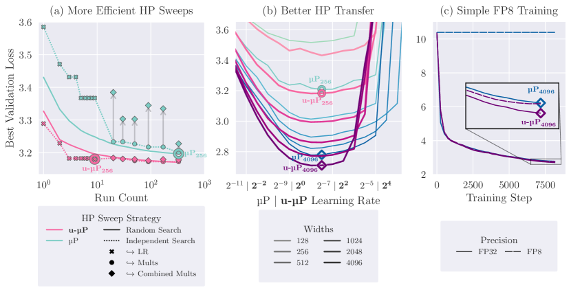
Figure 1: (a) Two different HP sweeping processes used for µP and u-µP proxy models. Unlike µP, u-µP admits independent (1D) search due to careful HP design. The first part of independent search is an LR sweep, which alone reaches near-optimal loss for u-µP. (b) Using the best proxy HPs from (a), we train many models at different widths and LRs. The best LR for width 256 is ~optimal for 4096, showing LR transfer along with lower loss. (c) We re-train with a simple un-scaled .to(float8) cast on matmul inputs. This would fail for other models, but u-µP trains with minimal degradation.

1 Introduction

The challenges of large-model training extend beyond the domain of engineering; they are also algorithmic in nature. Effective approaches for training smaller models are not guaranteed to work at the multi-billion-parameter scale used for today’s large language models (LLMs). These difficulties can be framed in terms of stability, which we consider in three forms:

1. feature learning stability, which ensures that parts of the model do not learn too fast or slow relative to each other.

2. hyperparameter stability, which ensures that the optimal HPs for small models remain unchanged as the model size grows.

3. numerical stability, which ensures that floating-point representations during training stay within the range of a given number format.

The Maximal Update Parametrization (µP) [1, 2] targets the first two sources of instability. µP defines a set of scaling rules that in principle make a model’s optimal HP values consistent across model sizes and ensure ‘maximal feature learning’ in the infinite-width limit. The practical benefits of this are that models continue to improve as they get larger, and that practitioners can re-use a set of HP values (especially the learning rate) found for a small proxy version of their model, on a larger target model. This is vital for modern LLM training, where the cost of sweeping over candidate HP values for the target model is prohibitive. Consequently, µP has been adopted by several open LLM training efforts [3, 4, 5, 6] and there are indications of its use in state-of-the-art LLMs.

However, there exists a gap between the extensive theory underpinning µP and its effective use in practice. This relates to issues surrounding efficient HP search, HP transfer, interpretability, ease-of-use and low-precision training. Some of these problems have been observed in the literature [9, 10, 2]; others we outline here for the first time. As a result, µP does not necessarily provide the kind of simple, stable scaling for which a user might hope.

To address this, we propose the Unit-Scaled Maximal Update Parametrization (u-µP). u-µP combines µP with another closely-related training innovation, Unit Scaling [11]. µP ideally provides consistent training dynamics across model sizes, but says little about what those dynamics should be. Unit Scaling addresses this by proposing an ideal principle for dynamics: unit variance for all activations, weights and gradients. Unit Scaling was initially designed to ensure stable numerics, but in the context of µP the principle of unit-scale brings many additional benefits. We show that it provides a foundation upon which the broader range of drawbacks identified for µP can be addressed.

1.1 Contributions

We focus on LLMs in this work as this is the domain where µP has primarily been used in the literature (though u-µP’s principles should extend to other architectures). We contribute the following:

1. Drawbacks of standard µP: We show that the way µP is typically applied has several limitations, and does not give effective transfer for Llama-style models (Section 3).

2. Simpler scaling rules: u-µP is easier to implement in practice than µP, and removes the unnecessary ‘base shape’ and initialization-scale HPs (LABEL:{sec:umup:combining_mup_with_us}; Table 2).

3. Out-of-the-box FP8 training: u-µP models generate tensors that lie close to the center of a floating point format’s range, meaning that most matrix multiplications can be performed in FP8 via a simple .to(float8) cast, with a minority requiring lightweight dynamic scaling for large-scale training (Section 4.2).

4. A principled, interpretable & independent set of HPs: The set of transferable HPs used in the µP literature is chosen in an inconsistent and arbitrary way. We provide concrete recommendations for a good set of transferable HPs to use with u-µP (Section 4.3).

5. Improved HP transfer: We identify a problem with the scaling of the embedding layer’s LR under µP. Fixing this for u-µP gives us better scaling with width (Section 4.4).

6. A more efficient approach to HP search: We show that u-µP facilitates a cheaper independent search method, attaining near-optimal loss when only sweeping the LR (Section 4.5).

We provide a guide for using u-µP in Appendix C, and a library [12] implementing u-µP functions, layers and optimizers, outlined in Appendix D.

2 Background

2.1 The Maximal Update Parametrization

Tensor Programs V [2] defines a parametrization as ‘a rule for how to change hyperparameters when the widths of a neural network change’. They show that µP is the only parametrization that gives ‘maximal feature learning’ in the limit, whereas standard parametrization (SP) has imbalanced learning (parts of the network blow up or cease to learn).

One consequence of this improved stability is that learning dynamics under µP are ideally independent of model-size, as are optimal HPs. This facilitates a method known as µTransfer, which describes the process of training many smaller proxy models to evaluate candidate HP values, then using the best-performing ones to train a larger target model. An HP is said to be µTransferable if its optimal value is the same across model-sizes.

ABC-parametrizations

µP, SP, and the Neural Tangent Kernel (NTK) [13] are all instances of abc-parametrizations. This assumes a model under training where weights are defined as:

$$w_{0} \sim\mathcal{N}(0,B_{W}^{2}),$$ (1)

$$W_{t} =A_{W}\cdot w_{t},$$

$$w_{t+1} =w_{t}+C_{W}\cdot\Phi_{t}(\nabla\mathcal{L}_{0},...,\nabla\mathcal{L}_{t}),$$

with $t$ a time-step and $\Phi_{t}(\nabla\mathcal{L}_{0},...,\nabla\mathcal{L}_{t})$ the weight update based on previous loss gradients.

A parametrization scheme such as µP is then defined specifying how scalars $A_{W},B_{W},C_{W}$ change with model width. This can be expressed in terms of width-dependent factors $a_{W},b_{W},c_{W}$, such that $A_{W}\propto a_{W}$, $B_{W}\propto b_{W}$, $C_{W}\propto c_{W}$. The values these factors take are what characterize a particular scheme. For µP these are given in Table 1. For depth a similar result has been proved using depth-µP [14], albeit in a restricted setting. When we refer to µP in the paper we assume the depth-µP scaling rules (Table 2, ‘Residual’ column).

A key property of the abc-parametrization is that one can shift scales between $A_{W},B_{W},C_{W}$ in a way that preserves learning dynamics (i.e. the activations computed during training are unchanged). We term this abc-symmetry. For a fixed $\theta>0$, the behavior of a network trained with Adam is invariant to changes of the kind:

$$A_{W}\leftarrow A_{W}\cdot\theta,\quad B_{W}\leftarrow B_{W}/\theta,\quad C_{W}\leftarrow C_{W}/\theta$$ (2)

(reproduced from Tensor Programs V, Section J.2.1). This means that parametrizations like µP can be presented in different but equivalent ways. ABC-symmetry is a key component in developing u-µP.

Table 1: The scaling rules defining µP. The type of a weight is determined by whether $\mathrm{fan{\text{-}}in}$ & $\mathrm{fan{\text{-}}out}$ both depend on width (hidden), only $\mathrm{fan{\text{-}}out}$ does (input), or only $\mathrm{fan{\text{-}}in}$ (output). Hence $\mathrm{fan{\text{-}}in}$ is always a multiple of width here.

	ABC-multiplier		Weight ($W$) Type
			Input	Hidden	Output
µP	parameter	($a_{W}$)	$\scriptstyle{1}$	$\scriptstyle{1}$	$\nicefrac{{\scriptstyle{1}}}{{\mathrm{fan{\text{-}}in}(W)}}$
	initialization	($b_{W}$)	$\scriptstyle{1}$	$\nicefrac{{\scriptstyle{1}}}{{\sqrt{\mathrm{fan{\text{-}}in}(W)}}}$	$\scriptstyle{1}$
	Adam LR	($c_{W}$)	$\scriptstyle{1}$	$\nicefrac{{\scriptstyle{1}}}{{\mathrm{fan{\text{-}}in}(W)}}$	$\scriptstyle{1}$

Transferable HPs

µP focuses on the subset of HPs whose optimal values we expect to transfer across axes such as width and depth. We term these µTransferable HPs. All µTransferable HPs function as multipliers and can be split into three kinds, which contribute to the three (non-HP) multipliers given by the abc-parametrization: $\alpha_{W},\sigma_{W},\eta_{W}$ where $A_{W}\propto\alpha_{W},B_{W}\propto\sigma_{W},C_{W}\propto\eta_{W}$. The difference between these multipliers and the ones that define a parametrization is that they are specified by the user, rather than being a function of width. $\alpha_{W}$ and $\eta_{W}$ are rarely introduced outside of the µP literature, but can be valuable to tune for both µP and SP models. In the µP literature the term ‘HPs’ often implicitly refers to µTransferable HPs. We adopt this convention here, unless specified otherwise.

Base shape

Two additional (non-µTransferable) HPs introduced by µP are the $\mathrm{base{\text{-}}width}$ and $\mathrm{base{\text{-}}depth}$. This refers to a mechanism where a user specifies a particular shape for the model, where its behavior under µP and SP are the same. The µP model still scales according to the abc-rules, so for all other shapes the two models will be different. This is implemented by dividing the µP scaling rules for the given model by those of a fixed-shape model at the $\mathrm{base{\text{-}}width}$ and $\mathrm{base{\text{-}}depth}$.

Putting this together with our abc-parametrization given in Equation 1, and the µTransferable HPs outlined above, we now derive our final, absolute expressions for $A_{W},B_{W},C_{W}$:

$$A_{W}\leftarrow\alpha_{W}\frac{a_{W}}{a_{W_{\textrm{base}}}},\quad B_{W}\leftarrow\sigma_{W}\frac{b_{W}}{b_{W_{\textrm{base}}}},\quad C_{W}\leftarrow\eta_{W}\frac{c_{W}}{c_{W_{\textrm{base}}}}$$ (3)

Though base shapes are necessary for µP, they are not typically swept. Rather, they are considered a preference of the user, who may wish to retain the behavior of an existing SP model at a given shape.

Choosing HPs to sweep

In theory, the search space of µTransferable HPs includes $\alpha_{W},\sigma_{W},\eta_{W}$ for every parameter tensor $W$ in the model. In practice far fewer HPs are swept, with global grouping often used for $\sigma_{W}$ and $\eta_{W}$, and many $\alpha_{W}$s dropped or grouped across layers.

The sets of HPs chosen for sweeps in the µP literature is explored in Section E.1. Tensor Programs V uses a random search to identify the best HP values, which has become the standard approach to sweeping. The number of runs in a sweep is typically in the low 100s, incurring a non-negligible cost (though usually less than a single training run of the target model). This high number partly owes to dependencies between HPs (shown in Section 5.2), making the search space hard to explore.

2.2 Low-precision training

All the major potential bottlenecks of model training—compute, communication and storage—see roughly linear improvements as the bit-width of their number format is reduced. In modern LLM training, the compute cost of large matrix multiplications (matmuls) means that substantial gains are available if these can be done in low-precision ($<32$ bit) formats. With the ending of Dennard scaling and Moore’s law [15, 16], the use of low-precision formats represents one of the most promising avenues towards increased efficiency in deep learning.

Recent AI hardware offers substantial acceleration for the 8-bit FP8 E4 and E5 formats. However the reduced range of these formats means that they cannot directly represent some values generated during training. Various methods have been introduced to address this, such as the per-tensor dynamic re-scaling in Transformer Engine [17]. However, this comes at the cost of added complexity and potential overheads. For a more in-depth treatment of low-precision formats, see Appendix J.

2.3 Unit Scaling

An alternative approach to low-precision training is Unit Scaling [11], which also uses fine-grained scaling factors to control range, but instead finds these factors via an analysis of expected tensor statistics at initialization. These are fixed factors, calculated independently of the contents of a tensor, at the beginning of training. As such, the method is easy to use and only adds the overhead of applying static scaling factors (which we show to be negligible in Appendix K).

These factors are chosen to ensure the unit variance of activations, weights and gradients at initialization. This is a useful criterion as it places values around the center of floating-point formats’ absolute range. This applies to all tensors, meaning every operation in the network requires a scaling factor that ensures unit-scaled outputs, assuming unit-scaled inputs. Unit Scaling does not provide a mechanism for re-scaling tensors dynamically during training, but due to its ideal starting scale for gradients, activations and weights this may not be required. Empirically this is shown to be true across multiple architectures, though it is not guaranteed.

We provide an example of deriving the Unit Scaling rule for a matmul op in Section E.2, resulting in the scaling factor: $1/\sqrt{d_{\mathrm{fan{\text{-}}in}}}$. We accompany this example with a full recipe for applying Unit Scaling to an arbitrary model.

3 The challenges with µP in practice

3.1 Not all training setups give µTransfer

Lingle [9] shows that directly applying µP to a decoder LM fails to provide LR transfer across width. Given that the primary use of µP in the literature has been LM training of this kind, this result suggests a significant limitation. How do we reconcile this with the strong LR transfer across width shown for language models in Tensor Programs V?

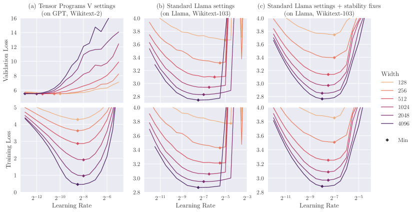
Figure 2: Effective µTransfer does not hold across all training setups. (a) We show strong transfer for the unrealistic setup used in Tensor Programs V (too many epochs; constant LR). (b) Moving to a more standard Llama training setup, transfer breaks down. (c) This is restored by the introduction of two stability fixes: non-parametric norms and independent weight decay.

We answer this Figure 2. The first training setup (a) is aligned with that used in Tensor Programs V (their Figure 4). There are several atypical aspects to their training setup, primarily the use of a constant LR schedule and a high number of epochs. This overfitting regime makes validation loss unusable, and transfer misleadingly good. When we remove these and shift to a standard Llama training setup (b), optimal HPs begin to drift with width. This confirms Lingle’s findings that standard µP is in fact a poor fit for modern LM training. We fix this (c) by the removal of parameters from LayerNorms/RMSNorms, as suggested by Lingle, and the introduction of independent weight decay for AdamW, as suggested by Wortsman et al. [18] . With these changes adopted, we recover the strong transfer shown in Tensor Programs V’s experiments.

3.2 It’s not clear which hyperparameters to sweep

The problem of selecting HPs to sweep can be framed as choosing a subset of the per-tensor $\alpha_{W},\sigma_{W},\eta_{W}$ HPs outlined in Section 2.1, and grouping across/within layers. As shown in Table 7, µTransfer experiments in the literature have done this in a variety ways. Practitioners have not justified these choices, appearing to rely on a mixture of precedent and intuition. We outline two major downsides to the lack of a principled approach.

Firstly, not all groupings of HPs are suitable. Consider the commonly-used global $\sigma_{\mathrm{init}}$ HP. At initialization the activations going into the FFN swish function have $\operatorname{std}(x_{\mathrm{swish}})\propto\sigma_{W_{\mathrm{gate}}}$, whereas the self-attention softmax activations have $\operatorname{std}(x_{\mathrm{attn}})\propto\sigma_{W_{\mathrm{Q}}}\sigma_{W_{\mathrm{K}}}$. A global $\sigma$ HP thus has a linear effect on the FFN and a quadratic effect on attention, suggesting that this grouping may be unideal.

Secondly, not all HPs are independent of one another. The key example of this is the interaction between $\sigma_{W}$ and $\eta_{W}$. The relative size of a weight update is determined by the ratio $\eta_{W}/\sigma_{W}$, not by either HP individually. Because of this, the optimal values for $\sigma$ and $\eta$ depend on each other, which we demonstrate empirically in Section 5.2. This can make the problem of HP search much harder, and may be why hundreds of random-search runs have been required for sweeps in the literature.

3.3 Base shape complicates usage

Most practitioners are unlikely to require alignment with an SP model, in which case it is unclear what $\mathrm{base{\text{-}}width}$ (and $\mathrm{base{\text{-}}depth}$) should be used. The literature has aligned on a standard $\mathrm{base{\text{-}}width}$ of $256$ (see Table 7), but this appears to lacking a principled motivation—though the fact that they are not dropped entirely suggests they may be beneficial under u-µP.

Implementing base-shape HPs (see Equation 3) can also add complications from an engineering perspective. The proposed implementation in the mup library [19] reflects this, requiring an extra ‘base’ model to be created and the original model to be re-initialized. This can interact awkwardly with other model-transforms for features like quantization, compilation, etc:

⬇

import mup

proxy_model = MupModel(d_model=128, …) # proxy width

base_model = MupModel(d_model=256, …) # base width

mup.set_base_shapes(proxy_model, base_model) # re-initialize proxy_model

3.4 µP appears to struggle with low-precision

Finally, we note an interesting contradiction observed in the relationship between µP and low-precision. One of the stated aims for µP is that its activations have $\Theta(1)$-sized coordinates in the limit [2, Desiderata J.1]. This desideratum is specifically given in order that values can be represented using finite-range floating-point numbers [1, Section 3]. Yet despite numerical stability being central to the theory underlying µP, this is not leveraged to ensure that µP models can actually be trained in low-precision. Indeed, for the LLM runs in Tensor Programs V the SP model trains successfully in FP16, while the µP model diverges (attributed to underflow of gradients). We remedy this with u-µP.

4 The Unit-Scaled Maximal Update Parametrization

In this section we show how µP can be adapted to satisfy Unit Scaling, and provide a new set of HPs which—thanks to Unit Scaling—are more interpretable and separable than those commonly used for µP, unlocking several practical benefits. For those wishing to apply u-µP to their own models, we provide a user-guide in Appendix C and an overview of our library implementing u-µP in Appendix D.

4.1 Combining µP with Unit Scaling

Whereas Unit Scaling provides rules for scaling all operations, µP only does so for parametrized ones. It’s these operations we need to address to arrive at a unified scheme, resolving differences in the scaling rules each recommends. We begin with the expressions for the $A_{W},B_{W},C_{W}$ scaling factors in Equation 3, and substitute in the µP scaling rules defined in Table 1. This results in a complete implementation of µP, which is shown in the top half of Table 2 (using the extended set of µP HPs given in Table 3). We set out to turn this into a valid Unit Scaling scheme, which requires unit initializations ($B_{W}\leftarrow 1$) and matmuls with the Unit Scaling factor we identified in Section 2.3 ($A_{W}\leftarrow 1/\sqrt{\mathrm{fan{\text{-}}in}}$).

Our first step is to drop the $\sigma_{W}$ and $\mathrm{base{\text{-}}fan{\text{-}}in}$ HPs entirely, and associate the $\alpha_{W}$ HPs with certain functions instead of weights—decisions we justify in the rest of this section (this results in the simplified intermediate implementation in Table 9). Our input weights now have unit initializations as desired, and a unit parameter multiplier, which is also the appropriate scaling factor (as input layers here are embedding lookups, not matmuls).

Hidden weights now have the implementation:

$$A_{W}\leftarrow 1,\quad B_{W}\leftarrow\frac{1}{\sqrt{\mathrm{fan{\text{-}}in}}},\quad C_{W}\leftarrow\eta\,\frac{1}{\mathrm{fan{\text{-}}in}},$$ (4)

which differs from our Unit Scaling criteria. However, using the abc-symmetry outlined in Equation 2 we can shift scales by a factor of $\sqrt{\mathrm{fan{\text{-}}in}}$, arriving at a unit-scaled scheme:

$$A_{W}\leftarrow\frac{1}{\sqrt{\mathrm{fan{\text{-}}in}}},\quad B_{W}\leftarrow 1,\quad C_{W}\leftarrow\eta\,\frac{1}{\sqrt{\mathrm{fan{\text{-}}in}}}.$$ (5)

Finally, our output layers also have unit initialization, but a parameter multiplier of $A_{W}\leftarrow 1/\mathrm{fan{\text{-}}in}$. This differs from the Unit Scaling rule, but in the forward pass this is permissible as there are no subsequent matmuls of a transformer. In the backward pass this mis-scaling would propagate, so we apply the desired $\leftarrow 1/\sqrt{\mathrm{fan{\text{-}}in}}$ factor. Using different forward and backward scales in this way is usually not allowed, but is valid for output layers due to the cut-edge rule (Appendix H).

The final change we make is to the input scaling rule, which we show in Section 4.4 is more effective if $A_{W}\leftarrow 1$ is replaced with $A_{W}\leftarrow 1/\sqrt{\mathrm{fan{\text{-}}out}}$ . With these changes made, we arrive at our final u-µP scheme, given in Table 2. It’s important to note that the scaling rules in this table must be combined with the standard Unit Scaling rules for other non-matmul operations. These are covered in Appendix B, and implemented in our library (see Appendix D).

Table 2: The definition of u-µP  along with an implementation of µP (assuming the extended HP set in Table 3). u-µP aims to simplify µP and provide the benefits of Unit Scaling.

	ABC-multiplier			Weight Type		Residual
			Input	Hidden	Output
	parameter	($A_{W}$)	$\alpha_{\mathrm{emb}}$	$1$ (or $\alpha_{\mathrm{attn}}$)	$\alpha_{\mathrm{out}}\frac{\mathrm{base{\text{-}}fan{\text{-}}in}}{\mathrm{fan{\text{-}}in}}$	$\sqrt{\frac{\mathrm{base{\text{-}}depth}}{0pt}}$*
µP	initialization	($B_{W}$)	$\sigma_{\mathrm{init}}$	$\sigma_{\mathrm{init}}\sqrt{\frac{\mathrm{base{\text{-}}fan{\text{-}}in}}{\mathrm{fan{\text{-}}in}}}$	$\sigma_{\mathrm{init}}$	—
	Adam LR	($C_{W}$)	$\eta\,\hat{\eta}_{\mathrm{emb}}$	$\eta\,\frac{\mathrm{base{\text{-}}fan{\text{-}}in}}{\mathrm{fan{\text{-}}in}}$	$\eta$	$\sqrt{\frac{\mathrm{base{\text{-}}depth}}{0pt}}$*
	parameter†	($A_{W}$)	$1$	$\frac{1}{\sqrt{\mathrm{fan{\text{-}}in}}}$	$\frac{1}{\mathrm{fan{\text{-}}in}}$‡	$\frac{1}{\sqrt{0pt}}$*
u-µP	initialization	($B_{W}$)	$1$	$1$	$1$	—
	Adam LR	($C_{W}$)	$\eta\,\frac{1}{\sqrt{\mathrm{fan{\text{-}}out}}}$	$\eta\,\frac{1}{\sqrt{\mathrm{fan{\text{-}}in}}}$	$\eta$	$\frac{1}{\sqrt{0pt}}$*
*Residual multipliers are applied to the end of each branch, rather than the output of linear layers.
†u-µP’s $\alpha$ HPs are associated with operations, not weights, so are not included here (see Section 4.3).
‡To maintain unit scale we apply $1/\sqrt{\mathrm{fan{\text{-}}in}}$ scaling in the backward pass (see Appendix H).

4.2 Out-of-the-box low-precision training

By applying the principles of Unit Scaling to µP, u-µP gains a key feature: the easy use of low-precision number formats during training. We can attribute the difficulties µP has with low precision to the fact that it ignores constant factors (along with weight and gradient-scaling), only ensuring that activations are of order $\Theta(1)$. The stricter condition of unit scale across all tensors at initialization provides a way of leveraging µP’s rules in order to make low-precision training work. During training, most scales in the model stabilize while certain tensors exhibit scale growth (see Section 5.5) and require a separate treatment in order to be cast to lower precision. The two solutions we propose here are either to use the E5M2 format to represent the larger scales or to apply a dynamic rescaling of the matmul input (Section 5.6 and Section 5.7 respectively).

4.3 A principled approach to hyperparameters

We saw in Section 3.2 that approaches for selecting which HPs to sweep are poorly motivated in the literature. Our objective in u-µP is to find a simple, well-justified and effective alternative. To this end, we propose the following ideal criteria:

1. Minimal cardinality: the use of as few HPs as possible.

2. Maximal expressivity: the ability to still express any model defined using the per-tensor $\alpha_{W},\sigma_{W},\eta_{W}$ HPs outlined in Section 2.1 (in practice, we relax this slightly).

3. Minimal interdependency: the optimal value of each HP should not depend on the value of other HPs, simplifying the search space.

4. Interpretability: there should be a clear explanation for what an HP’s value ‘means’ in the context of the model.

The u-µP HPs given in Table 3 are designed to satisfy these criteria, to the fullest extent possible. The placement of these HPs in the model is given in Table 6.

Table 3: Typical transformer HPs used under different schemes. Basic HPs in bold are considered most impactful and are commonly swept. Extended HPs in non-bold are not always swept, often set heuristically or dropped.

SP	µP	u-µP
$\bm{\eta}$	$\bm{\eta}$	$\bm{\eta}$
$\sigma\text{-}\mathrm{scheme}$	$\bm{\sigma_{\mathrm{init}}}$
	$\bm{\alpha_{\mathrm{emb}}}|\bm{\eta_{\mathrm{emb}}}$	$\alpha_{\mathrm{ffn\text{-}act}}$
	$\alpha_{\mathrm{attn}}$	$\alpha_{\mathrm{attn\text{-}softmax}}$
	$\alpha_{\mathrm{out}}$	$\alpha_{\mathrm{res}}$
	$\mathrm{base{\text{-}}width}$	$\alpha_{\mathrm{res\text{-}attn\text{-}ratio}}$
	$\mathrm{base{\text{-}}depth}$	$\alpha_{\mathrm{loss\text{-}softmax}}$

Cardinality & expressivity

We arrive at our set of HPs in three steps, starting with the full $\alpha_{W},\sigma_{W},\eta_{W}$ for each weight tensor $W$. Firstly, we can choose to ‘drop’ any one of these three HPs by permuting under abc-symmetry, such that one HP $=1$. As we want our weights to begin with unit scale, we choose $\sigma_{W}$ (i.e. $\theta=\sigma_{W}$ in Equation 2), leaving just $\alpha_{W},\eta_{W}$.

Secondly, we observe that several of the $\alpha_{W}$ HPs combine linearly with other $\alpha_{W}$ HPs, providing an opportunity to re-parametrize with a single HP. For instance, we noted in Section 3 that the scale of self-attention softmax activations is proportional to the product of $\sigma_{W}$ multipliers, and the same is true for $\alpha_{W}$ multipliers: $\operatorname{std}(x_{\mathrm{attn}})\propto\alpha_{W_{\mathrm{Q}}}\alpha_{W_{\mathrm{K}}}$. In this instance it appears more natural to use a single $\alpha$ parameter and associate it with the attention operation, rather than the weights. We term this $\alpha_{\mathrm{attn\text{-}softmax}}$.

We apply the same principle to the rest of the model, associating $\alpha$ HPs with operations instead of weights. This applies to all operations, unless they are unary and $k$-homogeneous for $k\geq 0$, in which case they propagate scale and don’t require an HP (see Section G.1). This results in the set of HPs shown, with their placement in the model given in Table 6.

Thirdly, we use a single global $\eta$ and group $\alpha$ HPs across layers. This breaks our expressivity criterion, but we argue represents the best trade-off between expressivity and cardinality. We show in Section A.2 that having tuned a global $\eta$ HP and our extended $\alpha$ HPs, the further benefits of tuning per-tensor $\hat{\eta}_{W}$ HPs (which modify the global $\eta$) is minimal, justifying our decision to only use one global $\eta$.

Interdependency

The second stage above, moving $\alpha$ HPs from weights into subsequent operations, not only reduces the number of HPs, but also minimizes the interdependence between those that remain. Interactions between HPs are complex and unlikely to be entirely separable, but we find that u-µP’s optimal HP values depend less on each other than under µP (see Section 5.2).

Interpretability

The combination of unit scale and reduced dependencies between HPs means that each $\alpha$ can be interpreted as determining some fundamental property of the model at initialization. For example, the $\alpha_{\mathrm{loss\text{-}softmax}}$ HP defines the (inverse of) the softmax’s temperature for a unit-scaled input. We also introduce a new scaling scheme (defined in Section G.2.2) for residual connections, designed to give HPs independence and a clear interpretation: $\alpha_{\mathrm{res}}$ defines the contribution of the residual connections to the output scale, and $\alpha_{\mathrm{res\text{-}attn\text{-}ratio}}$ defines the relative contribution of attention versus FFN branches. Finally, we choose not to include base shape HPs in u-µP. They do not add to expressivity, lack a clear interpretation (besides alignment to a base model at a particular shape), break the interpretations of other HPs (as given above), and complicate implementation.

4.4 A new embedding LR rule

Although theoretical transfer properties have been proved for µP, not all its HPs have had µTransfer shown empirically. We do so for the extended µP transformer HPs in LABEL:{fig:experiments:hp_transfer_over_width}, where we observe poor transfer across width for the embedding LR multiplier $\hat{\eta}_{\mathrm{emb}}$. The associated scaling rule for the embedding LR is constant in width ($c_{\mathrm{emb}}=1$), but this poor multiplier transfer suggests the rule is mis-specified. We show in Figure 3 (left) that a more effective rule is $c_{\mathrm{emb}}=1/\sqrt{\mathrm{fan{\text{-}}out}}$.

This keeps the optimal value of $\hat{\eta}_{\mathrm{emb}}$ the same regardless of width. Figure 3 (right) shows that a constant scaling rule leads to diminishing returns as width increases, whereas our new rule continues to work well at scale, attaining the same loss at 2048-width that constant scaling attains at 4096-width. Our adoption of this change is a key factor in the improved performance of u-µP over µP in Figure 1. We offer no theoretical justification for our rule, which we leave to further work.

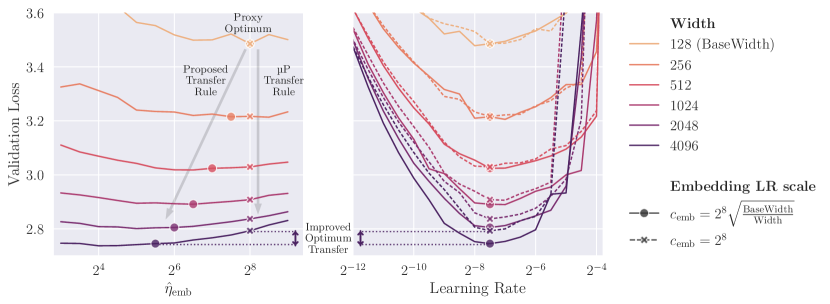
Figure 3: (Left) holding the embedding LR ($\hat{\eta}_{\mathrm{emb}}$) constant, vs. scaling with $\sqrt{\nicefrac{{\mathrm{base{\text{-}}width}}}{{\mathrm{width}}}}$, both with a fixed global LR. This suggests the µP embedding LR rule ($c_{\mathrm{emb}}$) should follow the latter scaling. (Right) we test this by sweeping the global LR under the two scaling rules. The new rule leads to lower loss on large models. (Dot/cross markers represent the same runs across both graphs).

4.5 Hyperparameter search

As shown in section Section 2.1, the standard approach to HP search for µTransfer is via a random sweep over all HPs simultaneously. Sweeping individual HPs separately is challenging due to the dependencies between them. In contrast, u-µP’s HPs are designed to admit such a strategy due to our interdependence criterion. Because of this, we propose a simpler sweeping strategy for u-µP which we term independent search (outlined in detail in Section A.4).

Independent search involves a sweep of the LR, followed by a set of one-dimensional sweeps of the other HPs (which can be run in parallel). The best results from the individual sweeps are combined to form the final set of HP values. We also consider an even simpler scheme, which only sweeps the LR, leaving other HP values at 1 (i.e. dropping them). For caution, we recommend the full approach, but in practice we find that only sweeping the LR is surprisingly effective, as shown in Figure 1 (a). This indicates that not only is the principle of unit scale good for numerics, but also for learning dynamics where it provides near-optimal scaling.

5 Experiments

5.1 Experimental setup

Our experiments all use the Llama [20] architecture trained on WikiText-103 [21] (excepting the large-scale runs in Section 5.7). We apply current best-practice LLM training techniques from the literature (full settings are given in Table 4). In accordance with our analysis of settings for µTransfer in Section 3.1, we remove parameters from norm layers, use independent AdamW, and avoid training on too many epochs for both u-µP and µP for the sake of fair comparison.

5.2 Quantifying hyperparameter interdependence

Our principled approach to HPs (Section 4.3) contains the requirement that their optimal values should depend minimally on the value of other HPs. We now investigate this empirically, conducting a 2D sweep over every pair of HPs for µP and u-µP, shown in Figures 9, LABEL: and 10 respectively.

To derive an empirical measure of HP dependency, we introduce the notion of transfer error (see Algorithm 1). This considers a pair of HPs, with one ‘fixed’ and the other for ‘transfer’. We take the best value of the transfer HP for each non-optimal value of the fixed HP, and use it with the optimal value of the fixed HP. The transfer error is the difference between the losses obtained and the minimum loss. Figure 4 shows this measure for each pair of HPs under µP and u-µP, reflecting the improvement in HP dependency as a result of our scheme. This gives u-µP a reduced risk of small transfer errors leading to large degradations, and the potential to sweep HPs in a more separable way.

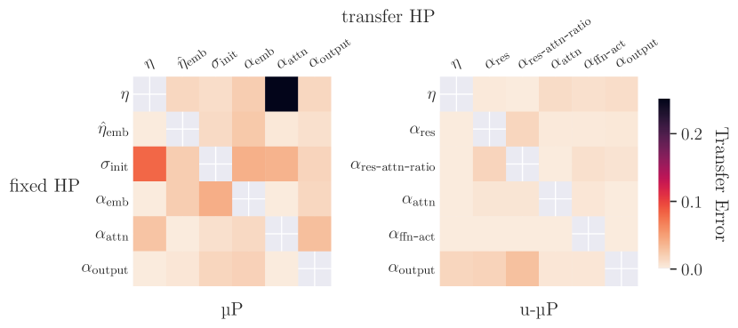
Figure 4: A visualization of the dependencies between pairs of HPs under each scheme. Transfer error measures the extent to which the optimal value of the transfer HP depends on the fixed HP (see Algorithm 1). On average, µP has a transfer error of 0.03, whereas u-µP has 0.005.

5.3 Hyperparameter search

We now leverage this improved separability of HPs for the purpose of efficient sweeping. In Figure 1 (a) we conduct a standard random search for µP and u-µP, along with the independent search outlined in Section 4.5 (and Section A.4). We observe the following:

1. For u-µP the LR-sweep phase of independent search alone is sufficient to reach near-optimal loss (totaling 9 runs). During this phase other HPs are fixed at 1, which for u-µP means that the inputs to operations are generally unit-scaled.

2. Consequently, we conclude that unit scale at initialization is close to the ideal scaling for effective learning here. This is not a property we asserted a priori, nor do we argue that it necessarily holds for other training setups and models; hence why we still provide a set of extended HPs to be swept.

3. In contrast µP still requires non-LR HPs to be swept to attain a reasonable loss. Unlike u-µP, fixing HPs at 1 results in arbitrarily-scaled inputs, which appear to result in worse training.

4. The ‘combined mults’ phase causes the loss to spike for µP. This is due to the HP dependencies shown in Figure 4, which mean HPs cannot be swept independently and used together. Conversely, lower dependence means this can be done for u-µP, making random search unnecessary.

5.4 Hyperparameter transfer

We demonstrate the transfer of LR across width in Figure 1 (b), of the other extended HPs across width in Figure 5, and of LR across training steps, batch size and depth in Figure 11. We find that:

1. The optimal LR is constant for all widths under u-µP, from 128 to 4096.

2. The optimal LR is also approximately constant for training steps, batch size and depth. This means we can scale our proxy model down across all these axes and maintain LR transfer. Of these, width appears the most stable and depth the least.

3. Whereas µP sees diminishing returns for larger widths, u-µP continues to benefit from width, with the 2048 u-µP model matching the 4096 µP model. We attribute this primarily to our improved embedding LR rule.

4. Non-LR HPs also have approximately constant optima across width under u-µP. This is not true for µP, where $\hat{\eta}_{\mathrm{emb}}$ has poor transfer due to the embedding scaling rule issue identified in Section 4.4, along with $\sigma_{\mathrm{init}}$ which in Section 3.2 we argue should not be grouped across all weights (and drop from the u-µP HP scheme).

5. The optimal values found for non-LR HPs are all close to 1. In practice this means that dropping these HPs entirely is potentially viable for similar models and training setups.

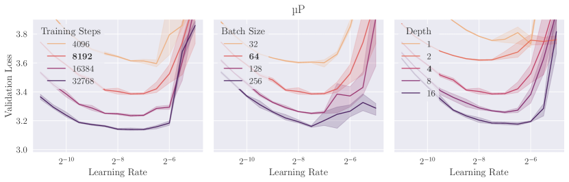
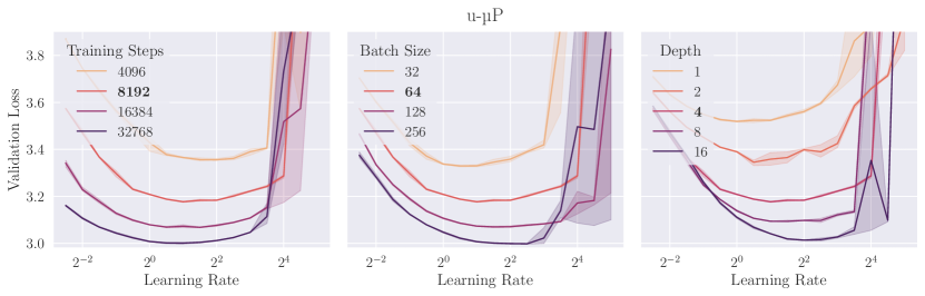
Figure 5: Learning rate transfer for µP (top) and u-µP (bottom), over training steps, batch size and depth. See Figure 1 (b) for transfer over width. The default shape parameter for other panels is shown in bold. The shaded area shows the $95\%$ confidence interval for the mean.

5.5 Numerical properties

Figure 6 shows the RMS over all linear modules in the model, Figure 13 shows RMS on a per-tensor basis over training steps, and Figure 14 shows the effect on RMS of LR, width, depth, steps and batch size. RMS captures the larger of the mean and scale of a distribution, and as such can be a good test of whether a tensor is likely to suffer over/underflow in low-precision number formats. Detailed analysis of these statistics is given in Section A.6, with our results supporting the central thesis of Unit Scaling: that tensors are well-scaled at initialization and largely remain so across training.

Based on these conclusions we propose our primary FP8 scheme: for every matrix multiplication, we cast the input, weight and grad-output tensors to E4M3, with the exception of the inputs to FFN and self-attention final projections, which are cast to E5M2 to accommodate their growing scale. This simply requires FP8 casts to be inserted into the model, avoiding the more complex scaling techniques used for FP8 in the literature (see Appendix J). This is possible due to the numerical stability we see in our analysis of u-µP. Additional details of our primary FP8 scheme are given in Section A.7.

As we demonstrate in Section 5.7, the primary scheme needs to be slightly adapted when model size, sequence length and number of training steps increase substantially.

5.6 FP8 training at smaller scale

We now show that u-µP can indeed be trained in our primary FP8 scheme in a smaller-scale setting (in terms of training tokens, rather than model-size). We note that our aim here is a proof-of-concept that this form of low-precision training can be done without degradation, not a demonstration of improved throughput which we leave to future work. To investigate the question of the potential benefits of FP8 training, Appendix K shows results for micro-benchmarking low-precision matmuls. We find that the addition of scaling factors adds no overhead, making our u-µP modifications essentially ‘free’.

Figure 1 (c) demonstrates the application of our FP8 scheme to model-training at width 4096. We use exactly the HPs suggested by the sweep in Figure 1 (a), but transferred to the larger model-width. µP fails entirely under our FP8 scheme due to gradient underflow, reflecting the requirement for different, and likely more complex scaling scheme. In contrast, u-µP trains in FP8 with only a small increase in validation loss versus the full-precision baseline.

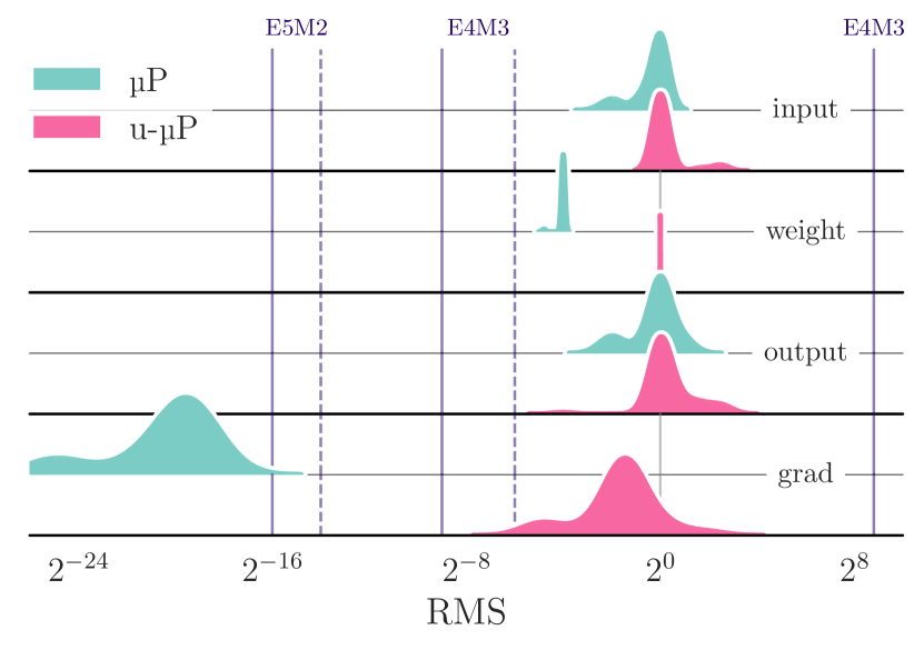
Figure 6: Per-tensor $\mathrm{RMS}=\sqrt{\sigma^{2}+\mu^{2}}$ across u-µP and µP models at initialization (left) and after training (right). u-µP tensors have RMS that starts close to $1$ and remains within E4M3 range at the end of training. Dashed and solid red lines show each format’s min. normal and subnormal values.

5.7 FP8 training at large-scale

The largest experiments in our above plots contain 1B parameters, but are trained at a smaller sequence length and number of steps than are typically used. Here we demonstrate that u-µP enables stable FP8 training for more realistic large-scale training scenarios, although some tweaks to our primary FP8 scheme are required, as outlined below. We use the same architecture as before, again following the training setup recommendations in Appendix C, and train our target models on 300B tokens of the publicly available SlimPajama dataset [22] (see Section A.8 for training details). We use three target model-sizes at approximately 1B, 3B and 7B parameters.

We begin with an independent search (Section 4.5) over our u-µP proxy model’s HPs. Here we make the following observations:

1. When using a relatively small proxy model with 8 layers and a width of 512 (4 attention heads), the HP-loss landscape is rather noisy. By doubling the width we are able to discern the optimal values of the HPs more clearly.

2. Learning rate $\eta$ and residual attention ratio $\alpha_{\mathrm{res\text{-}attn\text{-}ratio}}$ are the most important HPs. All other HPs can be left at their default value of $1$.

3. The optimal values of these HPs are $\eta=2^{3.5}$ and $\alpha_{\mathrm{res\text{-}attn\text{-}ratio}}=2^{-2.0}$ and thus differ non-trivially from the observed HPs in our previous experiments.

We also note that the previously-observed scale growth of inputs to FFN and self-attention final projections increases here. Directly casting inputs to FP8 fails in this setting, including when using E5M2 for extended numerical range. All other layers can still be cast to FP8 without problems (validated up to 3B scale), though we now require gradients to be in E5M2. To tackle the layers that exhibit scale growth, we fit them with a lightweight form of dynamic rescaling, leaving the rest of the model untouched.

The dynamic rescaling works as follows: Before the matrix multiplication, we normalize the input by its standard deviation and divide the result by the same scale afterwards, while ignoring both of these operations in the backward computation. We emphasize that this is still considerably less complex than the per-tensor scaling strategy that is usually required for FP8 training.

Using this refined FP8 scheme we perform two series of experiments:

1. On the 1B scale, we train a comparable SP model adopting the learning rate and initialization scheme from the Pythia model family [23], which we consider a strong established baseline. Apart from a standard training in BF16 mixed precision, we also try a simple FP8 cast and the Nvidia Transformer Engine framework [17] for this baseline. We then compare these SP models to three variants of our u-µP 1B model: One model in mixed precision, one model casting all layers except the critical ones to FP8 (our ‘partial’ scheme in Figure 7), and one where we apply our full FP8 scheme. Overall the u-µP models perform favorably (see Figure 7 (left)).

2. We train FP8 models up to 7B parameters using our full FP8 scheme. All runs converge (see Figure 7 right), and we expect our method to work at larger scales still.

Figure 7: (Left) Comparison of 1B training curves for u-µP and SP, using BF16 mixed precision vs FP8. Directly casting to FP8 causes SP to diverge, whereas u-µP still converges and outperforms the Transformer Engine FP8 baseline (SP FP8 T.E.). Using our proposed partial FP8 scheme, u-µP maintains nearly full performance compared to BF16 mixed precision. (Right) Loss curves from large scale training runs up to 7B using the u-µP FP8 scheme. Both figures use a smoothed running average loss with window size 100.

6 Related Work

Low-precision training

Techniques introduced to facilitate FP8 training include those covered in Appendix J and more [24, 25, 26]. These largely concern the quantizing of activations, weights and gradients, though [27] also explore FP8 optimizer states and cross-device communication, which we consider interesting avenues of further exploration. Recently, stable training has been demonstrated for the MX family of formats which use a shared block-exponent [28, 29], and even for the ternary BitNet format [30, 31, 32]. Again, we consider these formats for follow-up work.

Stability features

Another recent research trend has been the analysis of features that contribute to (or resolve) numerical and algorithmic instability. [18] show that unstable training dynamics can result from attention logit growth (fixed by QK-norm [33]) and from divergent output logits (fixed by z-loss [34]). [35] find large feature magnitudes can be avoided by zero-initialization, and loss spikes avoided via a modified AdamW, specifically for low-precision training. [36] investigate how pre-training settings affect instabilities revealed during post-training quantization. [37] apply a similar philosophy to Unit Scaling for the training of diffusion models, to address uncontrolled magnitude changes. Extreme activation values seen in large models [38, 39] have been addressed by softmax-clipping [40], and by the addition of extra terms [41] or tokens [42] to bias the attention computation. We do not adopt these features in our experiments to avoid confounding effects, but we expect them to benefit u-µP and hope to explore their usage.

Learning dynamics

Several recent efforts have tried to improve µP from different angles. [43] introduces the notion of the modular norm over the full weight-space, which like µP aims to ensure stable updates that provide LR transfer, and like u-µP is implemented via modules designed to ensure stable training. Challenging the assumptions underpinning µP, [44] explores the notion of alignment between parameters and data, demonstrating that other parametrizations with per-layer learning rates can outperform standard µP. We consider comparing these parametrizations against u-µP and trying unit-scaled versions valuable future work. Recent applications of µP to the problems of weight sparsity [45] and structured matrices [46] are also interesting candidates for u-µP.

7 Conclusions

We present an improved version of µP, underpinned by the principle of Unit Scaling. This provides the simple low-precision training that comes with unit-scale, but also provides a platform for solving other problems with µP. For instance, many HPs lack a clear interpretation under µP, but with u-µP we associate them with non-linear functions that have unit-scaled inputs, which means they can be understood as (inverse) temperatures. We build other improvements to the HP scheme on top of this, dropping the unnecessary and unhelpful base-shape HPs and $\sigma_{\mathrm{init}}$, and and minimizing dependencies between the remaining HPs.

This results in a simpler scheme to implement than µP, with several beneficial properties. A more efficient independent search can be done for proxy model HPs under u-µP, which can even drop non-LR HPs and still reach near-optimal loss. Our improved embedding LR scaling facilitates better performance at large widths, and we see strong HP transfer across width, depth, batch size and steps. Overall, u-µP simplifies and strengthens the practical application of µP, and provides further evidence that the principle of Unit Scaling is beneficial for model design.

8 Acknowledgments

We would like to thank Paul Balança, Andrew Fitzgibbon, Steve Barlow, Mark Pupilli, Jeremy Bernstein, Tim Large and Lucas Lingle for their feedback and discussions around u-µP at the various stages of its development.

Appendix A Additional experimental details

A.1 Experimental Setup

Our experimental analysis of u-µP was conducted by adapting the codebase used for Tensor Programs V, allowing us to compare µP and u-µP in the same setting. We change various experimental settings from the original paper to make our experiments better reflect standard training procedures, particularly the dataset which we switch from WikiText-2 to the larger WikiText-103 [21]. Where not specified otherwise, the default setting used in our experiments are given in Table 4. These also represent the settings of our proxy model.

Dataset	WikiText-103 [21]
Sequence length	$256$
Vocab size	$32000$
Training set tokens	$138\mathrm{M}$
Architecture	Llama [20]   (Transformer, PreNorm, RMSNorm, SwiGLU, RoPE, “untied” embeddings), non-trainable RMSNorm parameters.
Width	$256$   (scaled up to $4096$)
Depth	$4$
Number of heads	$4$   (scaled up to $64$)
Head dimension	$64$
Total parameters	$19.5M$   (scaled up to $1.07\mathrm{B}$)
Batch size	$64$
Training steps	$8192$ ($0.97$ epochs)
LR schedule	Cosine to $10\%$, $2000$ steps warm-up
Optimizer	AdamW $(\beta_{1},\beta_{2},\epsilon)=(0.9,0.999,10^{-8})$
Weight decay	$2^{-13}$, independent [47]
Dropout	$0.0$
µP HP search range	$\eta\in[2^{-10},2^{-6}]$
	$\hat{\eta}_{\mathrm{emb}}\in[2^{0},2^{8}]$
	$\sigma_{\mathrm{init}},\alpha_{\mathrm{emb}},\alpha_{\mathrm{{attn}}},\alpha_{\mathrm{output}}\in[2^{-2},2^{2}]$
u-µP HP search range	$\eta\in[2^{-1},2^{3}]$
	$\alpha_{\mathrm{attn}}\in[2^{-2},2^{2}]$
	$\alpha_{\mathrm{residual}},\alpha_{\mathrm{residual{\text{-}}attn{\text{-}}ratio}},\alpha_{\mathrm{ffn{\text{-}}act}},\alpha_{\mathrm{output}}\in[2^{-3},2^{3}]$
µP HP defaults	$\sigma_{\mathrm{init}}=\alpha_{\mathrm{emb}}=\alpha_{\mathrm{{attn}}}=\alpha_{\mathrm{output}}=\hat{\eta}_{\mathrm{emb}}=1$
u-µP HP defaults	$\alpha_{\mathrm{residual}}=\alpha_{\mathrm{residual{\text{-}}attn{\text{-}}ratio}}=\alpha_{\mathrm{ffn{\text{-}}act}}=\alpha_{\mathrm{output}}=\alpha_{\mathrm{attn}}=1$

Table 4: Default hyperparameters and training settings.

A.2 Per-tensor learning rates

In Section 4.3 we relax the requirement for each weight tensor in the u-µP model to have an associated tuneable learning-rate multiplier on top of the global learning rate. Whilst this does reduce the theoretical expressivity of the u-µP scheme, Figure 8 shows that using a single globally optimized learning rate is already at or close to the optimal choice for all weight tensors, and therefore it is reasonable to drop these multipliers in favor of reducing the number of HPs. However, a practitioner attempting to absolutely maximize the task performance of their model could experiment with tuning a few key per-tensor LRs, in particular the embedding table.

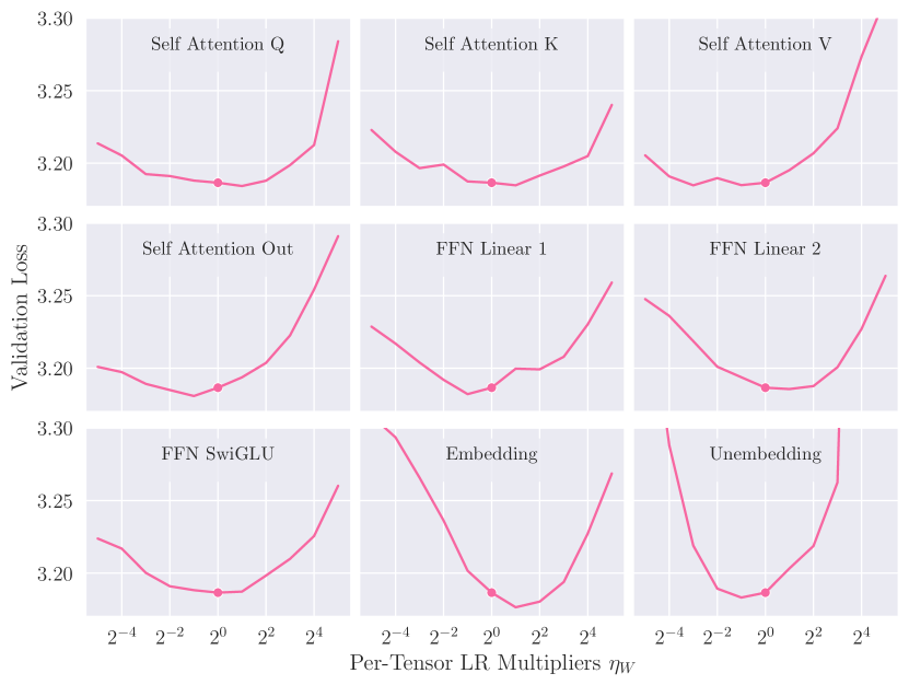
Figure 8: Independently varying per-tensor learning rate multipliers $\eta_{W}$, using the u-µP model of width 256 from Figure 1 with optimized global learning rate $2^{1.5}$ as the starting point. Where applicable, the same multiplier is used for tensors of the same name across transformer layers. Each subplot fixes all but one multiplier at 1, therefore the midpoint of each subplot is precisely the u-µP₂₅₆ model from Figure 1.

A.3 Hyperparameter independence

In Section 5.2 we explore the question of HP independence under µP and u-µP. The following plots in Figures 9, LABEL: and 10 show the result of a 2D sweep over every pair of HPs under each scheme. All other HPs are held at 1 when not swept, except the $\eta$ which is held at $2^{-7.5}$ for µP and $2^{1.5}$ for u-µP, and $\hat{\eta}_{\mathrm{emb}}$ which is held at $2^{4}$ for µP.

These results show visual dependence between µP hyperparameters as a diagonal structure in the grids, such as $(\hat{\eta}_{\mathrm{emb}},\sigma_{\mathrm{init}})$ and $(\eta,\alpha_{\mathrm{attn}})$. We quantify this in the plot in Figure 4, where we use a measure of HP dependence termed transfer error. This is explained verbally in Section 5.2, and we provide an algorithmic description in Algorithm 1. We note that differences in transfer error between the two methods may also be influenced by the flatness of the optimum. The HP and loss values used for our transfer error calculations are those in Figures 9, LABEL: and 10.

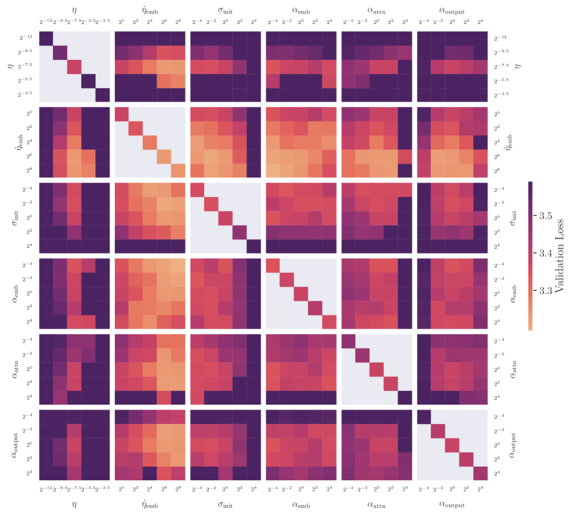
Figure 9: Hyperparameter coupling sweep for µP. Note strong coupling between optima, e.g. in the cases of $(\hat{\eta}_{\mathrm{emb}},\sigma_{\mathrm{init}})$ and $(\eta,\alpha_{\mathrm{attn}})$. See also: u-µP, Figure 10.

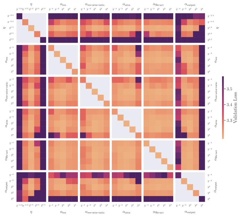
Figure 10: Hyperparameter coupling sweep for u-µP. Note less coupling than with µP, see Figure 9.

Algorithm 1 Transfer Error

A ‘fixed’ HP with candidate values $F=\{f_{1},\cdots,f_{n}\}$, a ‘transfer’ HP with candidate values $T=\{t_{1},\cdots,t_{m}\}$, a function that gives the final validation loss for the pair of HPs $L:F\times T\to\mathbb{R}$ (assuming all other HPs are fixed at default values).

$\mathrm{err}\leftarrow 0$

$f^{*},t^{*}\leftarrow\operatorname{argmin}(L)$

for $f$ in $F$ do

     if $f\neq f^{*}$ then

         $t\leftarrow\operatorname{argmin}(L(f))$

         $\mathrm{err}\mathrel{+}=L(f^{*},t)-L(f^{*},t^{*})$

     end if

end for

return $\mathrm{err}/(n-1)$

A.4 Hyperparameter search

Here we outline the particular search processes used for our µP and u-µP HP sweeps in Figure 1 (a). The random search samples uniformly from a grid defined over all extended HPs (extended HP sets are defined in Table 3, with grid values defined in Table 4). We perform the random search over 339 runs, each of which is a full training of the width-256 proxy model. We then simulate the effect of shorter searches at various run-counts by taking a random sample of the results, resulting in the smooth curve over run-count shown.

The independent search consists of the following phases:

1. Perform a 1D line search for an optimal learning rate, with other hyperparameters set to their default values ($9$ runs).

2. For each hyperparameter in parallel, perform a 1D line search ($330$ runs).

3. Combine the best settings from step 2, and re-evaluate ($6$ runs).

The number of runs in the 1D line search is an order of magnitude higher than is required in practice. We do so to form a fair comparison with the random search, which benefits from this large number of runs. The number of runs for the 1D line search could be reduced further by using binary search, though this would require sequential runs and limit the extent of parallelism.

A.5 Hyperparameter transfer experiments

LR transfer over width

The transfer experiments shown in Figure 1 (b) use the non-LR HPs found in Figure 1 (a) (indicated by the circled points), rather than using default HP values. For the u-µP sweep we take the HPs at the end of the LR portion of the independent search, as these are already close-to-optimal, and means only 9 runs were required in the sweep. In contrast, for µP it is necessary to use the results of the random search over a large number of runs.

LR transfer over other axes

For the training steps, batch size and depth transfer experiments in Figure 5, all HP values are fixed to 1 except LR which is swept. As with width transfer, u-µP outperforms µP here using these default HP values. Reducing training steps is done by fixing the number of warm-up steps (at 2000) and still cosine-decaying the learning rate to $10\%$; all that changes is the number of post-warm-up steps. We found this to be more effective than cutting-short the decay schedule. For both Figure 1 (b) and Figure 5 we sweep the LR over a logarithmically-spaced grid of step $2^{1/2}\times$, with 3 runs for each point.

Other HP transfer over width

For our non-LR HP transfer results in Figure 11, we note that good transfer under µP has not been demonstrated for all HPs used in the literature. This is particularly true for the $\hat{\eta}_{\mathrm{emb}}$ HP, which has poor transfer under µP. Our investigation here led to our identification of the need to adjust the embedding LR scaling rule outlined in Section 4.4. In many cases users have not swept this HP, but instead swept the corresponding parameter multiplier $\alpha_{\mathrm{emb}}$. How this HP interacts with the embedding LR scaling problem identified (and our proposed fix) remains to be explored, though we note in Figure 11 that it also appears to have poor transfer.

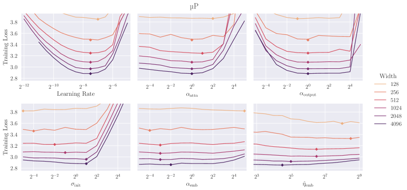
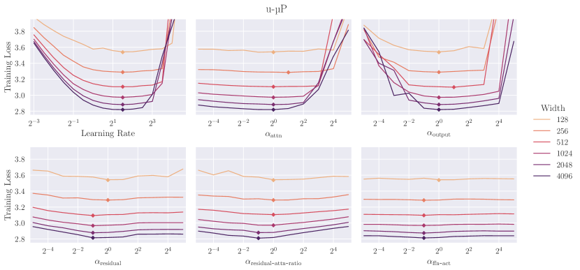
Figure 11: Transfer of model hyperparameters over width for µP (top) and u-µP (bottom). When one hyperparameter is being swept, all others are fixed at $1$, with the exception of Learning Rate $\eta=(2^{1.5},2^{-7.5})$ for (u-µP, µP).

Combined HP transfer

Whilst Figure 11 demonstrates the transfer of individual hyperparameters over width, Figure 12 instead demonstrates the simultaneous transfer of all hyperparameters when co-optimized on the small-scale proxy model, as is done for µTransfer. The µP and u-µP points are taken from Figure 1, with hyperparameters swept on a model of width 256 using a full random HP search and a simple learning rate sweep for µP and u-µP respectively. The Standard Parametrization scheme, as shown in Table 3 requires choosing a learning rate and a weight-initialization scheme. We follow the initialization scheme of GPT-NeoX [48], and transfer learning rate using a heuristic scaling factor of $\nicefrac{{\mathrm{base{\text{-}}width}}}{{\mathrm{width}}}$.

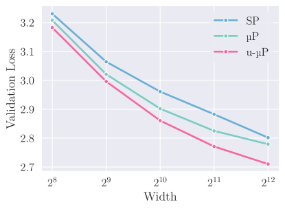
Figure 12: Transferring hyperparameters from width 256 up to 4096 using three different hyperparametrization schemes. µP and u-µP results are as seen in Figure 1, whilst Standard Parametrization follows the initialization approach of GPT-NeoX [48].

A.6 Numerical properties

Our analysis of the numerical properties of u-µP focuses on the RMS of tensors that we wish to cast to FP8: linear module input activations, weights and output gradients. From the RMS training statistics plots in Figure 6 and Figure 13 we note that

1. µP has gradients and weights with low RMS, at risk of FP8 underflow, whereas u-µP starts with $\mathrm{RMS}\approx 1$.

2. Many input activations do not grow RMS during training (due to a preceding non-trainable RMSNorm), however the attention out projection and FFN down projection have unconstrained input activations that grow considerably during training.

3. The decoder weight grows during training. Since it is preceded by a RMSNorm, the model may require scale growth in order to increase the scale of softmax inputs. Other weights grow slightly during training.

4. Gradients grow quickly but stabilize, except for attention out projection and FFN down projection, whose gradients shrink as the inputs grow.

We also evaluate how RMS growth is affected by model and training hyperparameters in the tensors that showed the highest end-training RMS, shown in Figure 14. This shows that the main parameter affecting scale growth is learning rate, with end-training RMS increasing to the right of the optimal LR basin, as training becomes unstable. End-training RMS is remarkably stable as width, depth, training steps and batch size are independently increased.

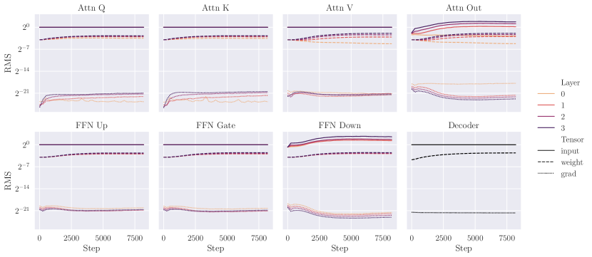
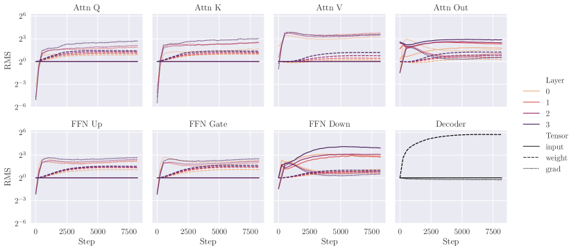
Figure 13: RMS during training, for all parametrized matmul inputs, for µP (top) and u-µP (bottom). Model width $256$, default hyperparameters, $\eta=(2^{1},2^{-8})$ for (u-µP, µP).

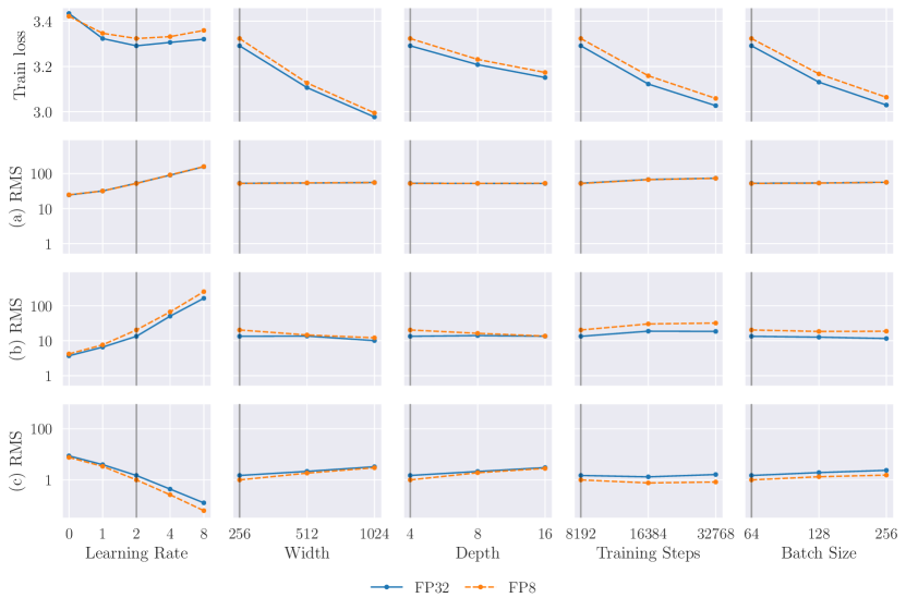
Figure 14: The effect of hyperparameters on FP8 training loss and on the end-training RMS of various tensors: (a) decoder weight, (b) last-layer FFN down-projection input and (c) last-layer FFN down-projection output gradient. Only learning rate has a substantial effect on the end-training RMS. Vertical lines show the default setting of that hyperparameter, as used for all other plots.

A.7 Our primary FP8 scheme

Each linear module in a model induces three matrix-matrix products: one during the forward pass to compute the output and two during the backward pass, computing gradients w.r.t. the weights and the inputs, respectively. The tensors participating in these matrix-matrix products are the input activations, the weights and the gradients w.r.t. the output activations.

We cast the input, weight and grad-output tensors to the narrower but more accurate E4M3 format, and for the two tensors which grow considerably across training—the inputs to FFN and self-attention final projections—we cast to the wider E5M2 format. The output of each matrix multiplication is produced directly in the higher-precision format (FP32 in our case), with no loss scaling or per-tensor scaling applied.

Unit scaling ensures RMS of 1 for all three tensors at initialization, and empirically the scales of these tensors do not drift too much during training, with the exception of the input tensors to the FFN and self-attention final projections, for which we use a wider format due to their increase in RMS over training steps (see Figure 13). Note that this scale growth is consistent across different HP settings (see Figure 14).

We have to adapt this scheme slightly for our large-scale training setup, which experiences increased scale-growth for the inputs to FFN and self-attention final projections, exceeding the range of E5M2. Our simple solution to this is a lightweight dynamic re-scaling for those particular problematic operations, still in FP8. This scheme is described in more detail in Section 5.7.

A.8 u-µP and FP8 at large scale

Our large-scale training settings are given in Table 5. These are largely the same as our standard experiments (Table 4), but with many more tokens used for training and scaling up to a larger model-size.

Dataset	SlimPajama [22]
Sequence length	$4096$
Vocab size	$65536$
Training set tokens	$600\mathrm{B}$
Architecture	Llama [20]   (Transformer, PreNorm, RMSNorm, SwiGLU, RoPE, “untied” embeddings), non-trainable RMSNorm parameters.
Width	$[2048,3072,4096]$   (1024 for proxy model)
Depth	$[16,24,32]$   (8 for proxy model)
Number of heads	$[16,24,32]$   (8 for proxy model)
Head dimension	$128$
Total parameters	$[1.07\mathrm{B},3.12\mathrm{B},6.98\mathrm{B}]$
Batch size	$1024$
Training steps	$72000$   ($\sim$ 300B tokens; $20000$ for proxy model)
LR schedule	Cosine to $10\%$, $500$ steps warm-up
Optimizer	AdamW $(\beta_{1},\beta_{2},\epsilon)=(0.9,0.95,10^{-8})$
Weight decay	$2^{-13}$, independent [47]
Dropout	$0.0$

Table 5: Large-scale training settings.

We use mixed-precision during training with optimizer states in FP32 that are sharded via ZeRO stage 1 [49]. We retain the model weights in BF16. Our FP8 scheme is as follows:

• In all matrix multiplications in the transformer block, we use E4M3 for the activation and the weight and E5M2 for the output gradient.

• For the attention dense projection and the FFN out projection we use dynamic rescaling as described in Section 5.7.

• In all remaining matrix multiplications we perform a simple FP8 cast with the aforementioned data types.

All other tensors remain either in BF16 (embedding, readout layer, norm, activation function) or FP32 (Flash Attention [50]).

Each model was trained on several Nvidia A100 (80GB) or H100 GPUs, with all FP8 experiments conducted on the H100 chips utilizing their native FP8 support. For the FP8 operations we use PyTorch’s torch._scaled_mm function as a backbone.

Appendix B Unit-scaled op definitions

Table 6: Implementations of unit-scaled ops, building on Table A.2. from the Unit Scaling paper [11]. These are considered part of u-µP and should be used in the place of standard operations.

Op	Unit Scaling factors
$\operatorname{matmul}(x,w)=xw$	$\alpha=\frac{1}{\sqrt{\mathrm{fan{\text{-}}in}}},\beta_{x}=\frac{1}{\sqrt{\mathrm{fan{\text{-}}out}}},\beta_{w}=\frac{1}{\sqrt{\mathrm{batch{\text{-}}size}}}$
$\operatorname{attention}(q,k,v)=$	$\alpha=\beta_{q}=\beta_{k}=\beta_{v}=$
$\quad\mathrm{softmax}\left(\alpha_{\mathrm{attn}}\,d_{\mathrm{head}}^{-1}\,(qk^{\top})\,\odot c_{\textrm{mask}}\right)v$	$\quad 1/\operatorname{log\_interpolate}\Bigl{(}\frac{1}{1+\frac{4d_{\mathrm{head}}}{\alpha_{\mathrm{attn}}^{2}}},1,\sqrt{\frac{\log(s)}{s}}\Bigr{)}$
$\operatorname{gated\_silu}(x_{\mathrm{in}},x_{\mathrm{gate}})=$	$\alpha=\beta_{x_{\mathrm{in}}}=\beta_{x_{\mathrm{gate}}}=$
$\quad x_{\mathrm{in}}\odot x_{\mathrm{gate}}\odot\operatorname{sigmoid}(\alpha_{\mathrm{ffn{\text{-}}act}}\,x_{\mathrm{gate}})$	$\quad 1/\operatorname{log\_interpolate}\Bigl{(}\frac{1}{1+\frac{1}{\alpha_{\mathrm{ffn{\text{-}}act}}^{2}}},\frac{1}{\sqrt{2}},\frac{1}{2}\Bigr{)}$
$\operatorname{residual\_add}(x_{\mathrm{resid.}},x_{\mathrm{skip}})=$	$a=\frac{\tau}{\sqrt{\tau^{2}+1}},\,b=\frac{1}{\sqrt{\tau^{2}+1}}\quad$
$\quad a\,x_{\mathrm{resid.}}+b\,x_{\mathrm{skip}}$	(see G.2.2 for full details, inc. values for $\tau$, which depends on $\alpha_{\mathrm{res}}$ and $\alpha_{\mathrm{res\text{-}attn\text{-}ratio}}$.)
$\operatorname{softmax\_xent}(x,t)=$
$\quad\operatorname{log\_softmax(\alpha_{\mathrm{loss\text{-}softmax}}\,x)}_{t}$	$\alpha=1,\;\beta=s/\sqrt{s-1}$
$\operatorname{RoPE}(x)$	$\alpha=\beta=1\quad$ (i.e. no scaling)
$\operatorname{RMSNorm}(x)$ (non-trainable, see [9])	$\alpha=\beta=1\quad$ (i.e. no scaling)

The original Unit Scaling paper provides scaling factors for various ops, in order to make them unit-scaled. However, these ops do not cover every case required for the Llama architecture used in our experiments, nor do they cover our updated residual layer implementation. To address this, in this section we outline a series of new unit-scaled ops for each of our required architectural features, as well as existing unit-scaled ops, as given in Table 6.

The presentation here is derived from that of the Unit Scaling Compendium given in [11, Table A.2]. This makes reference to the factors $\alpha,\beta_{1},\dots,\beta_{k}$. $\alpha$ is the output scaling factor in the forward pass, and $\beta_{i}$ are the scaling factors for the gradient of the op’s inputs in the backward pass. For each op, a value or rule is provided for determining the required mult to ensure unit-scale. The correct value for these multipliers is derived by analyzing the scaling behavior of each op, given some reasonable distributional assumptions about the input and incoming gradient tensors (see Section E.2 for an example). Below we provide an in-depth overview of each new or modified unit-scaled op we introduce here.

Unit-scaled dot-product attention

The Unit Scaling paper considers the attention layer scaling in terms of its separate components: the various matmul operations and the internal softmax. Linear operations are scaled using the standard rule, and the softmax scaling is given a $\alpha=\beta=s$ factor.

From an implementation perspective, the self-attention layer is more typically broken down into weight-matmuls and a fused scaled-dot-product attention operation. This is the case we handle here, accounting for three complicating factors not considered in the Unit Scaling paper:

1. As we use a decoder-style transformer in our experiments, our softmax operation has a causal mask applied to its input.

2. We follow the µP guidance of using $1/d_{\text{h}ead}$ scaling in our self-attention layer, rather than the usual $1/\sqrt{d_{\text{h}ead}}$.

3. We place a $\alpha_{\mathrm{attn}}$ multiplier immediately before the softmax, which is an HP that users may tune.

As a result our dot-product attention takes the form:

$$\operatorname{attention}(q,k,v) =\mathrm{softmax}\left(\alpha_{\mathrm{attn\text{-}softmax}}\cdot d_{\mathrm{head}}^{-1}\cdot(q\cdot k^{\top})\odot c_{\textrm{mask}}\right)\cdot v$$

The addition of an HP before the softmax introduces an additional challenge for Unit Scaling, as our scaling multipliers will need to account for this value when preserving unit scale.

This operation is sufficiently complex that we found an empirical model of its scale to be more accurate than any mathematically-derived rule (future work may consider justifying our model mathematically). We find that the scale of dot-product attention is approximately

$$\sigma(\operatorname{attention}(q,k,v)) =\operatorname{log\_interpolate}\left(\frac{1}{1+\frac{4d_{\mathrm{head}}}{\alpha_{\mathrm{attn}}^{2}}},1,\sqrt{\frac{\log(s)}{s}}\right)$$

where

$$\operatorname{log\_interpolate}(\alpha,b_{\mathrm{upper}},b_{\mathrm{lower}}) =e^{\alpha\log(b_{\mathrm{upper}})+(1-\alpha)\log(b_{\mathrm{lower}})}.$$

The corresponding scaling rule is therefore to divide by this factor in both the forward and backward pass, as outlined in Table 6.

SwiGLU FFN

Llama uses a SwiGLU [51] layer for its FFN, which introduces two new operations for us to unit-scale: a SiLU [52] (a.k.a. swish [53]) operation and an element-wise multiplication. We take a similar approach to our dot-product attention, and consider unit-scaling the following fused operation:

$$\operatorname{gated\_silu}(x_{\mathrm{in}},x_{\mathrm{gate}}) =x_{\mathrm{in}}\odot x_{\mathrm{gate}}\odot\operatorname{sigmoid}(\alpha_{\mathrm{ffn{\text{-}}act}}\,x_{\mathrm{gate}})$$

For the surrounding weight-matmuls we follow the standard Unit Scaling rules.

Again, we use an empirical model of the scale of this op, which is surprisingly similar to the dot-product attention model:

$$\sigma(\operatorname{gated\_silu}(x_{\mathrm{in}},x_{\mathrm{gate}})) =\operatorname{log\_interpolate}\left(\frac{1}{1+\frac{1}{\alpha_{\mathrm{ffn{\text{-}}act}}^{2}}},\frac{1}{\sqrt{2}},\frac{1}{2}\right),$$

dividing through by this factor to get our scaling rule.

Residual layers

Our implementation of residual layers for u-µP is more complex than other operations, as adjustments are required to:

1. Make pre-norm residual networks support Unit Scaling (see Appendix F).

2. Introduce our new, principled residual HPs (see Appendix G).

Our residual layer scheme is presented in full in G.2.2. For readers interested in our justification for this, see the sections noted above.

We also follow the example of Unit Scaling and delay the application of our residual multiplier in the backward pass to the base of the branch (see [11], Figure 3c). This does not change the model, and enables unit-scale to be maintained on the residual branch regardless of the value of the multiplier.

RoPE embeddings

We also require a unit-scaled implementation of Rotary Position Embeddings (RoPE [54]), which are applied just before the scaled dot-product attention operation. As RoPE essentially consists of pair-wise rotations of elements by different degrees, we observe no meaningful scale-change as a result of it’s application, and hence leave it unchanged.

RMSNorm

Following [9] we opt to use a non-trainable version of RMSNorm [55], in order to facilitate better transfer. As a result, we also leave this operation unchanged. Were a trainable RMSNorm to be used, the recipe would follow closely that of the LayerNorm presented in the original Unit Scaling Compendium.

Scale constraints

One final, minor deviation from the scheme outlined in the Unit Scaling paper is the way in which we apply scale constraints (see their Section 5.2). The essence of scale constraints is that for perfect unit scaling, sometimes the ideal scale for the forward pass differs from those in the backward pass. In some special cases (e.g. at the ends of the network) the use of different scales can be valid, but in the general case a single scale must be agreed upon. The solution in the Unit Scaling paper is to use the geometric mean of the forward and backward scales.

We propose instead to simply use the forward scale over the backward scale(s) in these cases. We do so for the following reasons:

1. For these architectures we find empirically that where there is a disparity in ideal forward and backward scales, it is not large.

2. By taking the forward scale, we can ensure strict unit-scale in the forward pass.

The value of the latter point is in terms of what it means for the interpretation of our u-µP multiplier HPs. Consider the $\alpha_{\mathrm{ffn{\text{-}}act}}$ multiplier; with strict unit scale we can say that the standard deviation of activations immediately before this multiplier is 1. Therefore the standard deviation immediately after is $\alpha_{\mathrm{ffn{\text{-}}act}}$. As this multiplier is (by design) the last operation before the ffn activation function, we can say that the interpretation of $\alpha_{\mathrm{ffn{\text{-}}act}}$ is simply to set the input standard deviation to the FFN’s activation function. Similar arguments can be made for other u-µP multiplier HPs. This interpretation only holds because we use the forward-scale in our constraints.

Appendix C A guide to using u-µP

We bring together our u-µP scheme presented in Section 4 to form a simple recipe for applying it to a model. The u-µP scheme is designed and validated on a Llama-style architecture, so it may not be applicable or effective on other models, particularly those with substantially different architectures. Exploring this question is an important avenue for future work.

Before applying our scheme, users are encouraged to apply the following pre-requisites to their training setup, based on our analysis of effective µTransfer in Section 3.1:

• Remove trainable parameters from normalization layers

• Use the independent form of AdamW

• Ensure training is in the under-fitting regime (i.e. avoid excessive data repetition)

Having done this, our recipe for using u-µP is as follows:

1. Replace operations & optimizers with u-µP versions: Each operation should be replaced by a unit-scaled version (these wrap the existing operations, with added static scales in the forward and backward passes). We have pre-calculated scales for common operations in Appendix B. Parameters should be initialized with unit variance, and Adam(W) adjusted to use the scaling rules defined in Section 4.4 (we refer to the optimizer as Adam in this section, but AdamW should be used if weight decay is required. Other optimizer scaling rules can be determined by the same process we outline). These features are all implemented in our library (see Appendix D).

2. Choose a set of HPs to sweep: From the set of HPs outlined in Table 3, select those to be swept. We recommend the extended set, though a basic LR sweep can be effective.

3. Decide on proxy model config: The cost of proxy model training should be such that the sweeping process is much less than target model training, while still being as representative as possible. We base our recommendations on the results in Figure 5. In general, width is the most reliable feature to transfer. Training steps and batch size also give good transfer, so moderate changes here are permissible. Depth is the least reliable feature for transfer, so we only recommend modest changes in depth. We keep the number of warmup steps constant, but always decay to the same final LR when varying the number of steps.

4. Perform independent HP search: Following the process outlined in Section 5.2 and Section A.4.

5. Train the target model: This can be done in FP8 simply by placing casts on matmul inputs (though for our large-scale experiments we found the scales of two operations drifted enough over time that some lightweight dynamic re-scaling was required).

The above functionality is provided in the Unit Scaling library, to avoid users having to implement it themselves, and to provide a reference implementation. We provide a guide to using this library in the following section.

Appendix D A guide to the unit scaling library

Our PyTorch [56] extension library, released under an open source license at https://github.com/graphcore-research/unit-scaling, accompanies this paper to provide standard and reference implementations of u-µP operations and optimizers.

This section provides an overview of the functionality of the library; please consult the repository documentation for details. A good place to start is our demo of a simple u-µP training implementation: https://github.com/graphcore-research/unit-scaling/blob/main/examples/demo.ipynb.

D.1 Standard usage

Compared with SP, u-µP requires the insertion of appropriate scaling factors in the forward and backward pass, a different parameter initialization scheme and the application of learning rate scaling rules based on the role and shape of each parameter.

The library provides implementations of ops in unit_scaling.functional with appropriate scaling rules (Table 6). Non-homogeneous ops (Section G.1) have optional mults, which are hyperparameters controlling shape of non-linear operations and the interpolation between mutiple inputs. Ops may also specify constraints, which are used to satisfy the cut-edge rule (Appendix H). Although this rule could be automated as a global graph transformation, the library makes constraint selection an explicit step for the user, while providing sensible defaults. For example, weight gradients are generally cut-edges, so are unconstrained.

Parameters are tagged with their role in the model (as a “bias”, “norm” parameter, “weight” or “output”). The library achieves this by extending torch.nn.Parameter with an additional property mup_type. This property is required for every parameter in a u-µP model. Given this, and information on the overall depth of the model, the library applies the learning rate rules of Table 2 as a pre-optimizer transformation that modifies the learning rate for each parameter. This allows standard PyTorch optimizers to be used without modification.

PyTorch uses modules to encapsulate parameter declaration, initialization and the calling of ops. The library makes available u-µP versions of common modules, which declare tagged parameters, apply unit-scale initialization, and call unit-scaled ops, with appropriate default settings.

With these components, user code for training using u-µP is very close to that of vanilla PyTorch (see an example in Figure 15).

⬇

import unit_scaling as uu

import unit_scaling.functional as U

model = uu.Linear(20, 10)

opt = uu.optim.AdamW(model.parameters(), lr=1.0)

opt.zero_grad()

U.mse_loss(model(input_), target).backward()

opt.step()

Figure 15: Using the unit scaling library given the tensors input_ & target.

D.2 Extending the library

As the set of deep learning ops of interest is always growing, the unit-scaling library is open for extension. For example, consider the possible implementation of unit-scaled hardtanh(x) = clip(x, -1, 1) in Figure 16.

⬇

import torch

from math import e, erf, pi, sqrt

from unit_scaling.constraints import apply_constraint

from unit_scaling.scale import scale_fwd, scale_bwd

def hardtanh(x, constraint="to_output_scale"):

y_scale = 1 / sqrt(1 - sqrt(2/(pi*e)))

grad_scale = 1 / sqrt(erf(1/sqrt(2)))

y_scale, grad_scale = apply_constraint(constraint, y_scale, grad_scale)

x = scale_bwd(x, grad_scale)

y = torch.nn.functional.hardtanh(x)

return scale_fwd(y, y_scale)

Figure 16: Implementing new unit-scaled operations.

The implementation follows a standard pattern:

1. Calculate the theoretical or empirical scaling factors for each forward and backward pass independently, based on independent unit-scaled Gaussian inputs.

2. Apply the optional constraint to select or combine these scaling factors, using the helper function apply_constraint.

3. Call scale_bwd on the inputs, and scale_fwd on the outputs to compensate for scaling after the op or grad-op is executed.

It can be checked empirically using random inputs and gradients (example in Figure 17).

⬇

x = torch.randn(2**20, requires_grad=True)

y = hardtanh(x, None)

y.backward(torch.randn_like(y))

assert abs(y.std() - 1) < 0.01

assert abs(x.grad.std() - 1) < 0.01

Figure 17: Testing unit-scaled operations, using constraint=None to allow independent fwd and bwd scaling. The default constraint "to_output_scale" preserves forward-pass scale while constraining the forward and backward scales to be equal.

D.3 As a reference implementation

The core technique of u-µP is readily implementable in most deep learning frameworks; the primary requirement is for custom gradient operations in order to provide equivalents of scale_fwd and scale_bwd. We hope that the library provides a useful reference, as well as a set of tools and techniques for developing custom u-µP support in other libraries and projects.

Appendix E Additional background material

E.1 The Maximal Update Parametrization

Theoretical background

We do not cover the theory underpinning µP in this paper, presenting only its resulting scaling rules (Table 1). For readers interested in this theory, the extensive Tensor Programs series [57, 58, 59, 60, 61] builds up a framework from which µP is derived [1]. For those requiring a more accessible introduction, [62] show that µP can be derived in a simpler and more general way by placing a spectral scaling condition on the norm of weights and their updates.

Approaches to HP sweeping in the literature

Table 7 outlines the ways in which users of µP in the literature have approached HP sweeping. These all follow the approach used in Tensor Programs V of a random sweep, sampling combinations from the joint space of all HPs. The authors of Tensor Programs V note that other more complex methods may be more efficient, but these are considered beyond the scope of their work and have not been used widely. A Bayesian search method was used for the development of MiniCPM [6], but the authors give no further details—as they use 400 runs in their sweep it is not clear that this approach makes HP search easier.

Table 7: Sweeping configurations used for a selection of µP models from the literature. The sweeping process is similar across models, the only differences being the choice of discrete or continuous distributions and their ranges.

Model	proxy/target tokens used	proxy/target model size	sweep size	base width	HPs swept
T.P.V WMT14 [2]	100%	7.1%	64	?	$\eta,\alpha_{\textrm{out}},\alpha_{\textrm{attn}}$
T.P.V $\text{BERT}_{\text{large}}$ [2]	10%	3.7%	256		$\eta,\eta_{\textrm{emb}},\alpha_{\textrm{out}},\alpha_{\textrm{attn}},\alpha_{\textrm{LN}},\alpha_{\textrm{bias}}$
T.P.V GPT-3 [2]	1.3%	0.6%	350		$\eta,\sigma,\alpha_{\textrm{emb}},\alpha_{\textrm{out}},\alpha_{\textrm{attn}},\alpha_{\textrm{pos}}$
MiniCPM [6]	0.008%	0.45%	400	256	$\eta,\sigma,\alpha_{\textrm{emb}},\alpha_{\textrm{residual}}$
Cerebras-GPT [3]	1.1%	1.5%	200	256	$\eta,\sigma,\alpha_{\textrm{emb}}$
SµPar [63]	6.6%	6.4%	350	256	$\eta,\sigma,\alpha_{\textrm{emb}}$

E.2 Unit Scaling

An example: the unit-scaled matmul op

Here we outline the procedure for calculating the scaling factor of a matmul op, which practitioners can use as a guide for scaling new ops that we do not cover in this paper (see Appendix B).

There are two potential approaches here. The first is to derive scaling factors from an analysis of an op’s dynamics. Specifically, given the assumption of unit-scaled inputs, the appropriate scaling factor is the reciprocal of the expected output scale. For a basic matrix-matrix matmul we have,

$$\operatorname{matmul}(X,W)=XW,\quad\quad X\in\mathbb{R}^{d_{\mathrm{batch}}\times d_{\mathrm{fan{\text{-}}in}}},\;W\in\mathbb{R}^{d_{\mathrm{fan{\text{-}}in}}\times d_{\mathrm{fan{\text{-}}out}}},$$

where weights and activations are sampled i.i.d. from a centered Gaussian:

$$X_{ij}\sim\mathcal{N}(0,\sigma_{X}^{2}),\;W_{jk}\sim\mathcal{N}(0,\sigma_{W}^{2}).$$

From this we can derive the expected output scale (i.e. $\sigma(\operatorname{matmul})$):

$$\operatorname{matmul}(X,W)_{ik}=\sum_{j=1}^{d_{\mathrm{fan{\text{-}}in}}}X_{ij}W_{jk},$$

$$\sigma\left(\operatorname{matmul}(X,W)_{ik}\right)=\sqrt{d_{\mathrm{fan{\text{-}}in}}}\,\sigma_{W}\,\sigma_{X}.$$

Under Unit Scaling we have $\sigma_{W}=\sigma_{X}=1$, and hence the scaling factor required to ensure a unit-scaled output is $1/\sqrt{d_{\mathrm{fan{\text{-}}in}}}$. This gives our final unit-scaled matmul:

$$\operatorname{u-matmul}(X,W)=\operatorname{matmul}(X,W)/\sqrt{d_{\mathrm{fan{\text{-}}in}}}$$

The distributional assumptions made here hold at initialization, but do not over training. A more precise model for the asymptotic behavior of neural networks under training is given by the Tensor Programs framework, but for the purposes of numerics this precise treatment of scale at initialization appears to be sufficient.

The second, less ideal approach to calculating scaling factors is to use experimentation to infer this relationship empirically. In this case, one would sample random initializations and compute the output scale over a range of $d_{\mathrm{fan{\text{-}}in}}$ values (or whatever HPs one expects the output scale to depend on), fitting a curve to the observed data.

Applying unit scaling

To apply Unit Scaling to a model and train in low-precision, the following steps are required:

1. Scale parameter initializations to have zero-mean and unit variance.

2. Replace operations with their unit-scaled equivalents (including and especially the loss, matmuls and residual-adds).

3. Constrain the scales of operations which are required to have the same forward and backward factors.

4. Place a simple .to(fp8) cast on the inputs to matmuls.

Step 3 relates to the problem of conflicting scales in the forward and backward passes. A single linear layer in a differentiated model requires 3 matmul ops in the forward and backward passes, each requiring a different scaling factor ($\frac{1}{\sqrt{d_{\mathrm{fan{\text{-}}in}}}},\frac{1}{\sqrt{d_{\mathrm{fan{\text{-}}out}}}},\frac{1}{\sqrt{d_{\mathrm{batch{\text{-}}size}}}}$). However, using these directly would give invalid gradients. The compromise here is that the activations and activation gradients have their scaling factors constrained such that they are equal (the original Unit Scaling paper recommends taking the geometric mean; we modify this for u-µP in Appendix B to simply use the forward scale everywhere). Weight gradients can still be given their own scaling factor due to the cut-edge rule (as explained in Appendix H).

Step 4 reflects the key benefit of Unit Scaling. Unlike other methods it changes the learning dynamics of a model, but the advantage is that unit-scaled models then ‘naturally’ generate well-scaled tensors. This means that low-precision arithmetic ideally becomes as simple as placing a cast operation before matmuls as outlined.

Appendix F Unit-scaled pre-norm residual layers

The popular pre-norm residual network architecture is simple to implement, but problematic to combine with Unit Scaling. It exhibits scale-growth in the skip-stream at initialization, due to the repeated addition of residual connections without subsequent normalization. Here we present a surprising and useful finding: that for any pre-norm model there exists a mathematically-equivalent model where this scale-growth is eliminated, through the careful re-scaling of residual connections.

Note that this section focuses on applying Unit Scaling to standard pre-norm models. Only once we have addressed this problem are we able to do the same for u-µP models, as shown in Section G.2. Readers only interested in our final u-µP residual implementation may skip ahead to Section G.2.2.

F.1 Scale growth in pre-norm residual networks

Let’s consider a pre-norm residual network of depth $L$:

$$R_{0}(x) =r_{0}x,$$ (6)

$$R_{l}(x) =r_{l}f_{l}(R_{l-1}(x))+R_{l-1}(x),\quad l=1,..,L$$ (7)

$$R_{L+1}(x) =f_{L+1}(R_{L}(x))$$ (8)

with embedding multiplier $r_{0}$ and residual branch multipliers $r_{l}$ for $l=1,..,L$. To satisfy pre-norm, all $f_{l}$ are zero-homogeneous functions, i.e. $f_{l}(\lambda x)=f_{l}(x)$.

The scale of the skip-stream at initialization as a result of Equation 7 is

$$\sigma(R_{l}) =\sqrt{r_{l}^{2}\sigma(f_{l})^{2}+\sigma(R_{l-1})^{2}}>\sigma(R_{l-1}),\quad l=1,..,L$$ (9)

assuming $r_{l}^{2}\sigma(f_{l})^{2}>0$. This shows that scale inevitably grows with the addition of each residual layer.

This scale-growth is clearly incompatible with unit scaling, which aims for $\sigma(R_{l})=1$ for all $l=0,..,L+1$. In the following we present an elegant solution to this problem making use of a symmetry transformation available in pre-norm residual architectures.

F.2 Residual symmetry in pre-norm architectures

To resolve the problem of scale shift in residual networks demonstrated by Equation 9, we try a slightly more general ansatz:

$$\hat{R}_{0}(x) =x,$$ (10)

$$\hat{R}_{l}(x) =a_{l}f_{l}(\hat{R}_{l-1}(x))+b_{l}\hat{R}_{l-1}(x),$$ (11)

$$\hat{R}_{L+1}(x) =f_{L+1}(\hat{R}_{L}(x))$$ (12)

with coefficients $a_{l},b_{l}$. We want to choose these coefficients so that the outputs of $\hat{R}_{l}$ are unit-scaled if the outputs $f_{l},\hat{R}_{l-1}$ are. A similar calculation as in Equation 9 leads to the sufficient condition

$$a_{l}^{2}+b_{l}^{2}=1,$$ (13)

which can be easily satisfied. Having restored Unit Scale, we are faced with another issue. It seems that Equations 10, 11 and 12 describe a different network than Equations 6, 7 and 8, whereas ideally the relation from input to final output should be unchanged when converting the network to Unit Scaling.

Note that the coefficients $a_{l},b_{l}$ are not uniquely defined yet, so our mathematical intuition tells us that we should find an additional constraint to get a unique solution. To find this constraint, let us consider our original residual network in Equations 6, 7 and 8 and analyze how the variance propagates through the network if we assume all the $f_{l}$ satisfy Unit Scaling and $\sigma(x)=1$. Let $\sigma_{l-1}^{2}$ denote the variance of $R_{l-1}$. Then a simple inductive calculation shows that

$$\sigma_{l-1}^{2}=\sum_{i=0}^{l-1}r_{i}^{2}.$$

By Equation 7 the output of $R_{l}$ adds a quantity of scale $r_{l}$ from the residual connection and a quantity of scale $\sigma_{l-1}$ from the skip connection. Intuitively, the ratio of these scales should be more important for the overall network dynamics than their absolute values. Thus our constraint becomes preserving the ratio of scales from the original model, through our choice of $a_{l},b_{l}$:

$$\frac{a_{l}}{b_{l}}=\frac{\sigma(r_{l}f_{l})}{\sigma_{l-1}}=\frac{r_{l}}{\sqrt{\sum_{i=0}^{l-1}r_{i}^{2}}}=:\tau_{l},$$

which, recalling Equation 13, (up to sign) uniquely defines our multipliers $a_{l},b_{l}$ as

$$a_{l}=\frac{\tau_{l}}{\sqrt{\tau_{l}^{2}+1}},\quad b_{l}=\frac{1}{\sqrt{\tau_{l}^{2}+1}}$$ (14)

In summary, we propose the modified residual network

$$\hat{R}_{0}(x) =x,$$ (15)

$$\hat{R}_{l}(x) =\frac{\tau_{l}}{\sqrt{\tau_{l}^{2}+1}}f_{l}(\hat{R}_{l-1}(x))+\frac{1}{\sqrt{\tau_{l}^{2}+1}}\hat{R}_{l-1}(x),$$ (16)

$$\hat{R}_{L+1}(x) =f_{L+1}(\hat{R}_{L}(x)),$$ (17)

$$\tau^{2}_{l} =\frac{r^{2}_{l}}{\sum_{i=0}^{l-1}r_{i}^{2}}.$$ (18)

Our main result of this section is that this network is indeed mathematically equivalent to the network defined in Equations 6, 7 and 8, under a simple additional structural assumption:

Lemma F.1.

Consider $R_{l}$, $\hat{R}_{l}$ defined as in Equations 7 and 16 respectively. Then $\hat{R}_{l}=R_{l}/\sqrt{\sum_{i=0}^{l}r_{i}^{2}}$ for all $l=0,..,L$.

Remarkably, this result does not assume the individual network operations $f_{l}$ actually satisfy Unit Scaling. It is purely a consequence of the pre-norm residual structure. However, only under Unit Scaling can the factors $\tau_{l}$ be interpreted as the ratio of scales between skip and residual branch.

As a consequence of the lemma, the final residual output $R_{L}(x)$ is the same as in our original network up to a fixed multiplier. Due to the zero-homogeneity of the final output function $f_{L+1}$ this gives $\hat{R}_{L+1}=f_{L+1}\left(R_{L}(x)/\sqrt{\sum_{i=0}^{l}r_{i}^{2}}\right)=f_{L+1}(R_{L}(x))=R_{L+1}$, proving the mathematical equivalence of our residual scheme. Modern LLM architectures like Llama [20] are pre-norm residual networks of this kind. Hence they admit a faithful unit-scaled reparametrization.

F.3 Proof of Lemma F.1

Proof.

This is proved by induction. For the base-case $l=1$, we have $\tau_{1}=r_{1}/r_{0}$, giving

$$\hat{R}_{1}(x) =\frac{\tau_{l}}{\sqrt{\tau_{l}^{2}+1}}f_{1}(x)+\frac{1}{\sqrt{\tau^{2}_{l}+1}}x$$

$$=(r_{1}f_{1}(x)+r_{0}x)/\sqrt{r_{0}^{2}+r_{1}^{2}}$$

$$=R_{1}/\sqrt{r_{0}^{2}+r_{1}^{2}}.$$

Then if the statement holds for $l-1$ we have

$$\hat{R}_{l}(x) =\frac{\tau_{l}}{\sqrt{\tau^{2}_{l}+1}}f_{l}(\hat{R}_{l-1}(x))+\frac{1}{\sqrt{\tau^{2}_{l}+1}}\hat{R}_{l-1}(x)$$

$$=\frac{r_{l}}{\sqrt{\sum_{i=0}^{l}r_{i}^{2}}}f_{l}(\hat{R}_{l-1}(x))+\frac{\sqrt{\sum_{i=0}^{l-1}r_{i}^{2}}}{\sqrt{\sum_{i=0}^{l}r_{i}^{2}}}\hat{R}_{l-1}(x)$$

$$=\left(r_{l}f_{l}(\hat{R}_{l-1}(x))+\sqrt{\sum_{i=0}^{l-1}r_{i}^{2}}\hat{R}_{l-1}(x)\right)/\sqrt{\sum_{i=0}^{l}r_{i}^{2}}$$

$$=\left(r_{l}f_{l}({R}_{l-1}(x))+\sqrt{\sum_{i=0}^{l-1}r_{i}^{2}}\frac{{R}_{l-1}(x)}{\sqrt{\sum_{i=0}^{l-1}r_{i}^{2}}}\right)/\sqrt{\sum_{i=0}^{l}r_{i}^{2}}$$

$$=\left(r_{l}f_{l}({R}_{l-1}(x))+{R}_{l-1}(x)\right)/\sqrt{\sum_{i=0}^{l}r_{i}^{2}}$$

$$=R_{l}(x)/\sqrt{\sum_{i=0}^{l}r_{i}^{2}}$$

∎

F.4 Unit Scaling for transformer residuals

The above scheme describes Unit Scaling for arbitrary pre-norm residual networks. We now apply it to the case of pre-norm transformer residual layers.

We can describe a transformer in terms of the residual network given in Equations 6, 7 and 8. Our $f_{l}$ functions alternate between self-attention layers and feed-forward layers. Implementations differ in the handling of how residual multipliers $r_{l}$ correspond to HPs. In many cases practitioners simply ignore these $r_{l}$, but for the sake of expressivity we assume the two types of residual layer each have their own HP, as well as the embedding. In other words,

$$r_{l}=\begin{cases}\alpha_{\mathrm{emb}}&l=0\\ \alpha_{\mathrm{attn{\text{-}}residual}}&l\textrm{ is odd }\\ \alpha_{\mathrm{ffn{\text{-}}residual}}&l\textrm{ is even, and }l>0.\end{cases}$$

To convert this to a Unit Scaled network we apply Equations 15, 16, 17 and 18, from which can derive the following closed-form expression for $\tau_{l}$:

$$\tau^{2}_{l}=\begin{dcases}\frac{\alpha^{2}_{\mathrm{attn{\text{-}}residual}}}{\alpha^{2}_{\mathrm{emb}}+\ell\alpha^{2}_{\mathrm{attn{\text{-}}residual}}+\ell\alpha^{2}_{\mathrm{ffn{\text{-}}residual}}}&l\textrm{ is odd }\\ \frac{\alpha^{2}_{\mathrm{ffn{\text{-}}residual}}}{\alpha^{2}_{\mathrm{emb}}+(\ell+1)\alpha^{2}_{\mathrm{attn{\text{-}}residual}}+\ell\alpha^{2}_{\mathrm{ffn{\text{-}}residual}}}&l\textrm{ is even}.\end{dcases}$$

where $\ell=\lfloor{\frac{l-1}{2}}\rfloor$.

This gives us a unit-scaled pre-norm residual implementation for a standard transformer, which is mathematically equivalent to a non-unit-scaled version. In the next section we augment this by adding in two HPs, in a carefully-designed manner that satisfies our criteria for u-µP HPs, giving us our full residual implementation.

Appendix G Justifying the u-µP hyperparameter scheme

Here we justify our particular choice of u-µP HP, as given in Table 3 (with their placement defined in Table 6). We discuss this topic briefly in Section 4.3, stating that all our HPs (excepting the LR) are $\alpha$ HPs, and under u-µP they are now associated with operations instead of weights. All operations have an $\alpha$ HPs, unless they are unary and $k$-homogeneous for $k\geq 0$.

We begin this section by explaining why we apply this rule to the model and how it results in three of our u-µP HPs. We then consider how best to hyperparametrize our residual layers, building on our criteria for HPs given in Section 4.3 and the unit-scaled pre-norm residual scheme in Appendix F.

G.1 Multipliers for non-homogeneous ops: $\alpha_{\mathrm{attn{\text{-}}softmax}},\;\alpha_{\mathrm{ffn{\text{-}}act}},\;\alpha_{\mathrm{loss{\text{-}}softmax}}$

In this section we derive the rest of our u-µP multipliers. We want to identify the minimal set that can still express all different choices of pre-op scales in the model. The crucial observation is that every pre-scale multiplier $\alpha$ of a unary operation $h\mapsto f(\alpha h)$ can be propagated through the network if $f$ is $k$-homogeneous for some $k>0$, i.e. $f(\alpha x)=\alpha^{k}f(x)$, leaving the model and its optimization unchanged. We can iterate this along the computational path until either the next operation is non-homogeneous, non-unary (we are at the end of a residual path), or the next operation is 0-homogeneous (e.g. a norm).

In the first case the accumulated scales are absorbed in the pre-op scale of the non-homogeneous operation (where we introduce a multiplier), in the second case they are absorbed in the residual addition for that branch (where we again introduce a multiplier), and in the final case the scale disappears (so we start over). We now go through the Llama forward computation and follow this paradigm to identify our multipliers in Table 8.

Table 8: A walkthrough of the Llama architecture, showing how our $\alpha_{\mathrm{attn{\text{-}}softmax}}$, $\alpha_{\mathrm{ffn{\text{-}}act}}$ and $\alpha_{\mathrm{loss{\text{-}}softmax}}$ multipliers are derived via an analysis of scale-propagation.

Op	Scale propagation behavior
Embedding	We show in Section G.2.1 that the embedding multiplier can be absorbed in the residual multipliers, meaning one is not required here.
Attention RMSNorm	This operation is $0$-homogeneous and thus we start over.
Query & key projection	Both are linear, meaning their scale is propagated. Multipliers are therefore not required.
Query-key matmul	Again linear. As query & key are both generated from the same input, this operation is $2$-homogeneous wrt. that input. Hence it also propagates scale.
Softmax	The softmax operation is non-homogeneous. Thus the pre-op scale of the softmax becomes our first multiplier: $\alpha_{\mathrm{attn{\text{-}}softmax}}$.
Value	The value layer is linear and hence propagates scale.
Softmax-value matmul	Again linear and hence propagates scale.
Attention projection	This operation is linear and lies at the end of the attention residual path. Hence there are no more multipliers in the attention block.
Residual add	This operation is non-unary and hence receives our second (and third) multipliers: $\alpha_{\mathrm{res}},\;\alpha_{\mathrm{res{\text{-}}attn{\text{-}}ratio}}$. The manner and motivation for using two multipliers here is justified in the next section.
FFN RMSNorm	This operation is $0$-homogeneous and thus we start over.
FFN input scale	The input layer is linear, hence it propagates scale.
Sigmoid input	This function is non-homogeneous and thus we have our fourth multiplier: $\alpha_{\mathrm{ffn{\text{-}}act}}$.
SiLU weight	This layer is also linear and propagates scale.
Product	The entry-wise multiplication of the outputs of sigmoid, input layer and SiLU weight is homogeneous and thus propagates scale.
FFN output	This layer is linear and at the end of the residual path. Hence there are no more multipliers in the FFN residual block.
Residual add	See above.
Output RMSNorm	This operation is $0$-homogeneous and thus we start over.
Output head	This layer is linear, hence it propagates scale.
Loss	The cross-entropy loss is non-homogeneous and leads to our final multiplier: $\alpha_{\mathrm{loss{\text{-}}softmax}}$.

G.2 Residual branch multipliers: $\alpha_{\mathrm{res}},\;\alpha_{\mathrm{res{\text{-}}attn{\text{-}}ratio}}$

In this section we derive our two u-µP residual HPs. We start with the basic, non-unit scaled model we began with in the previous section, outlined in Equations 6, 7 and 8. We described a set of $\alpha_{\mathrm{emb}},\alpha_{\mathrm{attn{\text{-}}residual}},\alpha_{\mathrm{ffn{\text{-}}residual}}$ HPs associated with this model in Section F.4. However these HPs poorly satisfy our cardinality, independence and interpretability criteria from Section 4.3, so in the Section G.2.1 we present a re-parametrization of these HPs designed to better satisfy these points. In Section G.2.2 we then combine these HPs with the final unit-scaled pre-norm residual scheme we derived in Appendix F, resulting in our complete u-µP residual scheme.

G.2.1 Improved hyperparameters for transformer residuals

To avoid cluttered notation, in this section we rename

$$\alpha_{\mathrm{res}}=\alpha_{r},\quad\alpha_{\mathrm{res{\text{-}}attn{\text{-}}ratio}}=\alpha_{\rho}$$

$$\alpha_{\mathrm{emb}}=\alpha_{e} ,\quad\alpha_{\mathrm{attn{\text{-}}residual}}=\alpha_{a}\quad\alpha_{\mathrm{ffn{\text{-}}residual}}=\alpha_{f}.$$

To make the presentation more clear, we derive our new HPs using the standard residual scheme from Equations 6, 7 and 8. For the actual unit scaled implementation one needs to transform the multipliers following Equations 15, 16, 17 and 18, which we do in Section G.2.2.

To facilitate our analysis, we can view the transformer residual output as the sum of three terms:

$$R_{L} =R_{L}^{(e)}+R_{L}^{(a)}+R_{L}^{(f)},$$

$$R_{L}^{(e)} :=\alpha_{e}x,$$

$$R_{L}^{(a)} :=\sum_{l=1}^{L/2}\frac{\alpha_{a}}{\sqrt{L/2}}f_{2l-1}(R_{2l-1}(x)),$$

$$R_{L}^{(f)} :=\sum_{l=1}^{L/2}\frac{\alpha_{f}}{\sqrt{L/2}}f_{2l}(R_{2l}(x)),$$

and define the average residual scale,

$$\sigma(R_{L}^{(a,f)})^{2}:=\frac{\sigma(R_{L}^{(a)})^{2}+\sigma(R_{L}^{(f)})^{2}}{2}.$$

Note that we have added in the depth-µP multipliers here, though a similar analysis can be performed for non-depth-µP models. As above, $f_{l}$ functions alternate between self-attention layers and feed-forward layers.

With respect to our interpretability criterion, we propose two new multipliers that correspond to dynamics in the network which we suggest are important to control at initialization. The first is the ratio of the average scale of the residuals’ contributions to those of the embedding, $\alpha_{r}=\sigma(R_{L}^{(a,f)})/\sigma(R_{L}^{(e)})$. The second is the ratio of the scale of the attention-residuals’ contributions to those of the feed-forward-residuals, $\alpha_{\rho}=\sigma(R_{L}^{(a)})/\sigma(R_{L}^{(f)})$. Not only do these two ratios control key dynamics of our model, but we can use them to replace our existing $(\alpha_{e},\alpha_{a},\alpha_{f})$ multipliers.

Let us first examine these two quantities for a standard (non-unit-scaled model). Residual functions of the same kind have the same expected output scale at initialization in pre-norm networks, meaning we can denote the output scale $\sigma(f_{l}(R_{l}))$ of all self-attention functions as $\sigma_{a}$, and of all feed-forward functions as $\sigma_{f}$. We thus have the following scales at the output:

$$\sigma(R_{L}^{(e)}) =\alpha_{e}\sigma(x),$$

$$\sigma(R_{L}^{(a)}) =\frac{\alpha_{a}}{\sqrt{L/2}}\,\sigma\!\left(\sum_{i=1}^{L/2}f_{2l-1}(R_{2l-1})\right)=\alpha_{a}\sigma_{a},$$

$$\sigma(R_{L}^{(f)}) =\frac{\alpha_{f}}{\sqrt{L/2}}\,\sigma\!\left(\sum_{i=1}^{L/2}f_{2l}(R_{2l})\right)=\alpha_{f}\sigma_{f},$$

$$\sigma(R_{L}^{(a,f)}) =\sqrt{\frac{(\alpha_{a}\sigma_{a})^{2}+(\alpha_{f}\sigma_{f})^{2}}{2}}.$$

Recalling our definitions of $\alpha_{r},\alpha_{\rho}$ above, this gives us:

$$\alpha_{\rho} =\frac{\alpha_{a}}{\alpha_{f}}\frac{\sigma_{a}}{\sigma_{f}},$$

$$\alpha_{r} =\sqrt{\frac{(\alpha_{a}\sigma_{a})^{2}+(\alpha_{f}\sigma_{f})^{2}}{2\,(\alpha_{e}\sigma(x))^{2}}},$$

$$=\sqrt{\frac{\alpha_{\rho}^{2}+1}{2}}\frac{\sigma_{f}}{\sigma(x)}\frac{\alpha_{f}}{\alpha_{e}}.$$

The original $\alpha_{a},\alpha_{f}$ multipliers can then be written in terms of $\alpha_{r},\alpha_{\rho}$:

$$\alpha_{a} =\alpha_{\rho}\alpha_{f}\frac{\sigma_{f}}{\sigma_{a}}$$

$$\alpha_{f} =\alpha_{r}\alpha_{e}\frac{\sigma(x)}{\sigma_{f}}\sqrt{\frac{2}{\alpha_{\rho}^{2}+1}}$$

We have replaced two of the three original multipliers, but still have a dependence on $\alpha_{e}$ here in our expressions for $\alpha_{f}$ and $R_{L}^{(e)}$, which we now remove by dividing it out of our residual branches and embedding. We use the hat ($\hat{\cdot}$) symbol to denote terms that have been divided-through by $\alpha_{e}$. This new system of equations is equivalent to our old one thanks to the zero-homogeneity of the final post-residual layer:

$$R_{L+1}(x) =f_{L+1}(R_{L}^{(e)}+R_{L}^{(a)}+R_{L}^{(f)})$$

$$=f_{L+1}((R_{L}^{(e)}+R_{L}^{(a)}+R_{L}^{(f)})/\alpha_{e})$$

$$=f_{L+1}(\hat{R}_{L}^{(e)}+\hat{R}_{L}^{(a)}+\hat{R}_{L}^{(f)})$$

This gives $\hat{R}_{L}^{(e)}=\alpha_{e}x/\alpha_{e}=x$, removing our first occurrence of $\alpha_{e}$. Following the division through $\hat{R}_{L}^{(a)}$ and $\hat{R}_{L}^{(f)}$, we obtain:

$$\hat{R}_{L}^{(a)} :=\sum_{l=1}^{L/2}\frac{\hat{\alpha}_{a}}{\sqrt{L/2}}f_{2l-1}(R_{2l-1}),$$

$$\hat{R}_{L}^{(f)} :=\sum_{l=1}^{L/2}\frac{\hat{\alpha}_{f}}{\sqrt{L/2}}f_{2l}(R_{2l}),$$

$$\hat{\alpha}_{a} =\alpha_{\rho}\hat{\alpha}_{f}\frac{\sigma_{f}}{\sigma_{a}},$$

$$\hat{\alpha}_{f} =\alpha_{r}\frac{\sigma(x)}{\sigma_{f}}\sqrt{\frac{2}{\alpha_{\rho}^{2}+1}}.$$

This system of equations is the same as the original, but with the two $\alpha_{e}$ terms dropped, meaning our model’s multipliers can be expressed in terms of only $\alpha_{r}$ and $\alpha_{\rho}$. Using the above equations, any pair of values for $(\alpha_{r},\alpha_{\rho})$ can be translated back into an equivalent set of values for $(\alpha_{e},\alpha_{a},\alpha_{f})$ such that the output $R_{L+1}(x)$ is the same, meaning that our multipliers are no less expressive than the original set. This satisfies our desired criteria of minimizing the number of multipliers while maintaining expressivity.

We can simplify further in the case of unit-scaled models, which are designed such that $\sigma(x),\sigma_{a},\sigma_{f}$ are all $1$ at initialization. In this case our re-parametrization becomes:

$$\hat{\alpha}_{a} =\alpha_{\rho}\hat{\alpha}_{f},$$ (19)

$$\hat{\alpha}_{f} =\alpha_{r}\sqrt{\frac{2}{\alpha_{\rho}^{2}+1}},$$ (20)

$$\hat{\alpha}_{e} =1.$$ (21)

This is the basis of our claim that Unit Scaling is what enables a more intuitive set of multipliers. Not only do the multipliers $\alpha_{r}$ and $\alpha_{\rho}$ represent important dynamics in the network at initialization (the ratio of residual-to-embedding scales, and the ratio of attention-to-feed-forward scales), but it’s only via unit scaling that these equations become simple enough to implement in practice. Using equations Equations 19, 20 and 21 for a non-unit scaled network may still be effective, but the interpretation we’ve given to $\alpha_{r}$ and $\alpha_{\rho}$ no longer hold.

Our final desired property is an empirical one: that the most effective choice of one multiplier depends as little as possible on the choice of the other multiplier(s). We demonstrate that our multipliers satisfy this property better than the standard set of residual multipliers in Section 5.2.

G.2.2 The full u-µP residual scheme

Here we give the full definition of our u-µP residual scheme, summarizing the results of previous sections. A general pre-norm transformer is implemented as:

$$R_{0}(x) =c\,x,$$ (22)

$$R_{l}(x) =a_{l}f_{l}(R_{l-1}(x))+b_{l}R_{l-1}(x),\quad l=1,..,L$$ (23)

$$R_{L+1}(x) =f_{L+1}(R_{L}(x)),$$ (24)

where $a_{l},b_{l}$ and $c$ are scalar multipliers, and the $f_{l}$ alternate between self-attention and feed-forward layers. We consider our baseline set of µP residual HPs here to be $(\alpha_{\mathrm{emb}},\alpha_{\mathrm{attn{\text{-}}residual}},\alpha_{\mathrm{ffn{\text{-}}residual}})$, which we implement (assuming depth-µP branch scaling) as:

$$a_{l} =\begin{dcases}\frac{\alpha_{\mathrm{attn{\text{-}}residual}}}{\sqrt{L/2}}&l\textrm{ is odd (self-attention)}\\ \frac{\alpha_{\mathrm{ffn{\text{-}}residual}}}{\sqrt{L/2}}&l\textrm{ is even (feed-forward)}\end{dcases}$$

$$b_{l} =1$$

$$c =\alpha_{\mathrm{emb}}.$$

The corresponding u-µP set of residual HPs is $(\alpha_{\mathrm{res}},\alpha_{\mathrm{res{\text{-}}attn{\text{-}}ratio}})$, which we implement as:

$$a^{2}_{l} =\frac{\tau^{2}_{l}}{\tau^{2}_{l}+1}$$ (25)

$$b^{2}_{l} =\frac{1}{\tau^{2}_{l}+1}$$ (26)

$$c =1,$$ (27)

$$\tau^{2}_{l} =\begin{dcases}\frac{\hat{\alpha}^{2}_{a}}{\frac{L}{2}+\ell\hat{\alpha}^{2}_{a}+\ell\hat{\alpha}^{2}_{f}}&l\textrm{ is odd}\\ \frac{\hat{\alpha}^{2}_{f}}{\frac{L}{2}+(\ell+1)\hat{\alpha}^{2}_{a}+\ell\hat{\alpha}^{2}_{f}}&l\textrm{ is even}\end{dcases},\quad\ell=\left\lfloor{\frac{l-1}{2}}\right\rfloor$$ (29)

$$\hat{\alpha}^{2}_{a} =\alpha^{2}_{\mathrm{res{\text{-}}attn{\text{-}}ratio}}\,\hat{\alpha}^{2}_{f}\$$ (30)

$$\hat{\alpha}^{2}_{f} =\frac{2}{\alpha_{\mathrm{res{\text{-}}attn{\text{-}}ratio}}^{2}+1}\,\alpha^{2}_{\mathrm{res}}\,.$$ (31)

This is the u-µP residual scheme. It satisfies the three properties that we initially set out to achieve: the variance at initialization of our $R_{l}(x)$ is always 1, our HPs have a clear and useful interpretation, and our scheme is as expressive as the baseline (which is neither unit-scaled or has interpretable HPs).

Appendix H The cut-edge rule

In the section we review the notion of constraints used for scaling operations in a computational graph. For a more thorough, generalized treatment, please refer to Section 5.1 and Appendix E.4 of the original Unit Scaling paper [11].

For simplicity, we will only discuss the cut-edge rule in the context of a typical neural network. For each operation $f$, parametrized by $\theta$ taking input $x$ and emitting output $y$, a user must choose how to scale $y$, $\nabla_{x}$ and $\nabla_{\theta}$ (gradient of loss w.r.t. $x$ and $\theta$ respectively). In the simplest case, where there are no further data dependencies, we can simply choose factors that preserve unit scale. In more complex scenarios, we must balance the need for each tensor to be unit-scaled and for gradients to be correct up to a constant factor.

In particular, a problem emerges in the presence of residual blocks in which $y=x+f(x;\theta)$. In these circumstances, $\nabla_{x}$ is computed as the sum of residual gradient $\nabla_{f}$ $\frac{\partial{f}}{\partial{x}}$ and skip gradient $\nabla_{y}$. If we choose not to insert scaling factors into our graph, $\nabla_{f}$ $\frac{\partial{f}}{\partial{x}}$ and $\nabla_{y}$ will have some ratio of scale $r$. However, if we have chosen to rescale the gradient of operations in $f$, then $\nabla_{f}$ $\frac{\partial{f}}{\partial{x}}$ will have been rescaled by some $s$. This means the new ratio of $\nabla_{f}$ $\frac{\partial{f}}{\partial{x}}$ and $\nabla_{y}$ will be $r\cdot s$. Therefore, when adding these together, $\nabla_{x}$ is no longer a correct gradient up to a constant factor.

How do you remedy this? If we can ensure that the scaling factors are the same for both the input gradients and outputs of an op, we will have $s=1$. This ensures that gradients for inputs to residual blocks are correct up to a constant factor.

How do you decide when you are free to preserve unit scale, and when to constrain scaling factors to be the same? We previously define the cut-edge rule [11] for computational graphs where nodes represent forward pass operations and edges represent operation outputs. If an input edge is a cut-edge, i.e., the number of connected components in the graph would increase upon deletion (examples in a typical transformer model: output of embedding gather, output of a residual add, output of final norm, output token logits, weights), there is no need to constrain the scales of the operation’s output edge and the input edge gradient. For all other input edges (e.g., inputs to a residual add, intermediates computed along a residual branch), the scales of gradients and outputs should be constrained.

Appendix I From µP to u-µP

Here we outline additional details to help readers follow the process of deriving u-µP from the combination of Unit Scaling and µP. Our first step of dropping $\sigma_{W}$ and $\mathrm{base{\text{-}}fan{\text{-}}in}$, and moving $\alpha_{W}$s to functions, results in Table 9. This intermediate scheme does not yet satisfy Unit Scaling, but simplifies the HP rules in preparation for further changes. Note that we have also removed $\hat{\eta}_{\mathrm{emb}}$ as we don’t include this HP in our u-µP extended HP set. We have included residual scaling rules here, in accordance with depth-µP, which we intend u-µP to satisfy, though our standard µP implementation doesn’t use it.

Table 9: An intermediate scheme resulting from dropping those HPs from µP which are not needed under u-µP.

ABC-multiplier			Weight Type		Residual
	Input	Hidden	Output
parameter	($A_{W}$)	$1$	$1$	$\frac{1}{\mathrm{fan{\text{-}}in}}$	$\frac{1}{\sqrt{0pt}}$*
initialization	($B_{W}$)	$1$	$\frac{1}{\sqrt{\mathrm{fan{\text{-}}in}}}$	$1$	—
Adam LR	($C_{W}$)	$\eta$	$\eta\,\frac{1}{\mathrm{fan{\text{-}}in}}$	$\eta$	$\frac{1}{\sqrt{0pt}}$*

Appendix J Low-precision and its trade-offs

Number formats for deep learning

The standard numerical representations used in deep learning are the set of formats defined by the IEEE 754 floating-point standard [64]. IEEE floats comprise three elements: a sign bit, exponent bits, and mantissa bits. The number of exponent bits determines the range of a format, while the mantissa determines the precision. We refer readers to the original Unit Scaling paper ([11], Section 3.1) for a comprehensive overview of floating-point representations.

The default format used for training is the single-precision floating-point format, commonly known as FP32, with some hardware providers automatically casting it to the smaller TF32 compute mode for accelerated arithmetic. The 16-bit FP16 and BF16 formats were later introduced, and more recently the FP8 E5 & E4 formats [65, 66, 67]. The higher range of E5 has typically been used for gradients, while the higher precision of E4 has been seen as necessary for weights and activations. Our particular implementation of FP8 training is covered in Section A.7. Other aspects of training such as the optimizer state and cross-device communication have also been put into FP8 [27], though not all tensors are amenable to being run in the lowest precision [38] without degradation. The use of multiple formats is known as mixed precision [68]. A comparison of these formats is given in Table 10.

Table 10: A comparison of deep learning formats. E indicates exponent bits, and M mantissa bits. The smaller formats typically give more FLOPS, at the expense of reduced range and/or precision.

Format	E	M	| max |	| min normal |	| min subnormal |	FLOPS (vs TF32)
FP32	8	23	$3.4\times 10^{38}$	$1.2\times 10^{-38}$	$1.4\times 10^{-45}$	$<1\times\hphantom{<}$
TF32	8	10	$3.4\times 10^{38}$	$1.2\times 10^{-38}$	$1.1\times 10^{-41}$	$1\times$
BF16	8	7	$3.4\times 10^{38}$	$1.2\times 10^{-38}$	$9.2\times 10^{-41}$	$2\times$
FP16	5	10	$65504$	$6.1\times 10^{-5\hphantom{0}}$	$6.0\times 10^{-8\hphantom{0}}$	$2\times$
FP8 E5	5	2	$57344$	$6.1\times 10^{-5\hphantom{0}}$	$1.5\times 10^{-5\hphantom{0}}$	$4\times$
FP8 E4	4	3	$448$	$1.6\times 10^{-2\hphantom{0}}$	$2.0\times 10^{-3\hphantom{0}}$	$4\times$

The benefits of low-precision

Using numerical representations with fewer bits facilitates the design of more efficient arithmetic in hardware, typically leading to a linear increase in peak FLOPS (as shown in Table 10). As large-scale training efforts are typically compute-bound due to the size of matmuls [69], putting the inputs to these operations in low-precision formats has a substantial impact on training efficiency. Low-precision formats also reduce the other two common performance constraints: for memory-bandwidth-bound models they require fewer bits to be transmitted, and for memory-size-bound models they require fewer bits to be stored.

The challenges of low-precision

Unfortunately, moving to low-precision formats also increases quantization error. For values within the representable range this takes the form of rounding error, and for values outside it, clipping error (both overflow and underflow). Rounding error tends to be an intrinsic problem: the number of mantissa bits dictates the expected accuracy of representations and this cannot easily be changed. In contrast, clipping error is often eliminated by scaling a tensor so that its values lie within the range of a format. Note that a multiplicative change in values of this kind doesn’t affect the (relative) rounding error, due to the exponential spacing of values. Most research into making low-precision work has focused on the problem of scaling tensors in this way.

Simply casting all tensors to FP16 or FP8 tends to impair training, largely due to clipping error. For FP16, this primarily affects gradients. [68] address this by introducing a fixed global loss-scale HP, which multiplies the loss value in the backward pass, artificially up-scaling gradients to lie within FP16 range [68]. Automatic loss scaling [70] builds upon this idea, making the loss-scale a dynamic value that is tuned during training.

The later BF16 format has the same range as FP32, making loss scaling unnecessary. For FP8 no such range-equivalent format can exist, so the problem of clipping error must be addressed. Most FP8 implementations have done so by moving from a global loss-scale to a local scale for each FP8 tensor. In pseudo-code, this takes the form:

⬇

a = scale(A)

b = scale(B)

A = to_fp8(A / a)

B = to_fp8(B / b)

C = (a * b) * matmul(A, B)

where we assume that matmul takes inputs in FP8 and directly produces the output in higher precision.

The result of the scale() operation can either be a fixed scale determined before training [66], or in the case of Transformer Engine [71], computed dynamically as a function of the ‘absmax’ of the input tensor (though they introduce a delay across time-steps, to facilitate an efficient fused kernel). Increasing granularity and computing scales dynamically using this kind of method inevitably adds complexity (from both a logical and implementation perspective), as well the potential for computational overhead. Unit Scaling generally avoids the need for matmul input scaling.

Appendix K Benchmarking scaled matrix multiplication implementation in PyTorch

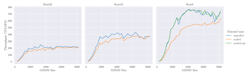
Figure 18: Square matrix multiplication throughput in TFLOPs with and without scaling factors applied to the output across 32-, 16-, and 8-bit float dtypes on NVIDIA H100 PCIe. Naive implementation in PyTorch.

Standard strategies for FP8 training require expensive statistics gathering (e.g., amax) per tensor. A key benefit of u-µP for FP8 training is that it instead provides us with static scaling factors to rescale operation outputs. Even a naive implementation in pytorch can achieve a minimal drop in hardware utilization.

Figure 18 demonstrates hardware utilization for FP8, FP16, and FP32 matrix multiplications on a single NVIDIA H100 PCIe card. For FP16 and FP32, torch.matmul is used, whereas torch._scaled_mm is used for FP8. Comparing "scaled" to "unscaled" matrix multiplication demonstrates a 30$\%$, 20$\%$, and 10$\%$ drop in hardware utilization for each data type respectively. In the case of FP8, where the drop in utilization is most pronounced, utilization can be recovered by passing the scaling factor as a scale associated with one of the two input tensors.

It should be noted that as of PyTorch version 2.3, torch._scaled_mm always computes amax as well as the matrix multiplication. The performance of FP8 matrix multiplications could be higher without this overhead.

References

- [1] Greg Yang and Edward J. Hu. Tensor programs IV: Feature learning in infinite-width neural networks. In Marina Meila and Tong Zhang, editors, Proceedings of the 38th International Conference on Machine Learning, ICML 2021, 18-24 July 2021, Virtual Event, volume 139 of Proceedings of Machine Learning Research, pages 11727–11737. PMLR, 2021.
- [2] Greg Yang, Edward J. Hu, Igor Babuschkin, Szymon Sidor, Xiaodong Liu, David Farhi, Nick Ryder, Jakub Pachocki, Weizhu Chen, and Jianfeng Gao. Tensor programs V: Tuning large neural networks via zero-shot hyperparameter transfer. CoRR, abs/2203.03466, 2022.
- [3] Nolan Dey, Gurpreet Gosal, Zhiming Chen, Hemant Khachane, William Marshall, Ribhu Pathria, Marvin Tom, and Joel Hestness. Cerebras-GPT: Open compute-optimal language models trained on the cerebras wafer-scale cluster. CoRR, abs/2304.03208, 2023.
- [4] Nolan Dey, Daria Soboleva, Faisal Al-Khateeb, Bowen Yang, Ribhu Pathria, Hemant Khachane, Shaheer Muhammad, Zhiming Chen, Robert Myers, Jacob Robert Steeves, Natalia Vassilieva, Marvin Tom, and Joel Hestness. BTLM-3B-8K: 7B parameter performance in a 3B parameter model. CoRR, abs/2309.11568, 2023.
- [5] Zhengzhong Liu, Aurick Qiao, Willie Neiswanger, Hongyi Wang, Bowen Tan, Tianhua Tao, Junbo Li, Yuqi Wang, Suqi Sun, Omkar Pangarkar, Richard Fan, Yi Gu, Victor Miller, Yonghao Zhuang, Guowei He, Haonan Li, Fajri Koto, Liping Tang, Nikhil Ranjan, Zhiqiang Shen, Xuguang Ren, Roberto Iriondo, Cun Mu, Zhiting Hu, Mark Schulze, Preslav Nakov, Tim Baldwin, and Eric P. Xing. LLM360: Towards fully transparent open-source LLMs. CoRR, abs/2312.06550, 2023.
- [6] Shengding Hu, Yuge Tu, Xu Han, Chaoqun He, Ganqu Cui, Xiang Long, Zhi Zheng, Yewei Fang, Yuxiang Huang, Weilin Zhao, Xinrong Zhang, Zhen Leng Thai, Kai Zhang, Chongyi Wang, Yuan Yao, Chenyang Zhao, Jie Zhou, Jie Cai, Zhongwu Zhai, Ning Ding, Chao Jia, Guoyang Zeng, Dahai Li, Zhiyuan Liu, and Maosong Sun. MiniCPM: Unveiling the potential of small language models with scalable training strategies. CoRR, abs/2404.06395, 2024.
- [7] OpenAI. GPT-4 technical report. CoRR, abs/2303.08774, 2023.
- [8] xAI. Grok-1. https://github.com/xai-org/grok-1, 2024.
- [9] Lucas D. Lingle. A large-scale exploration of -transfer. CoRR, abs/2404.05728, 2024.
- [10] Ebtesam Almazrouei, Hamza Alobeidli, Abdulaziz Alshamsi, Alessandro Cappelli, Ruxandra Cojocaru, Mérouane Debbah, Étienne Goffinet, Daniel Hesslow, Julien Launay, Quentin Malartic, Daniele Mazzotta, Badreddine Noune, Baptiste Pannier, and Guilherme Penedo. The Falcon series of open language models. CoRR, abs/2311.16867, 2023.
- [11] Charlie Blake, Douglas Orr, and Carlo Luschi. Unit scaling: Out-of-the-box low-precision training. In Andreas Krause, Emma Brunskill, Kyunghyun Cho, Barbara Engelhardt, Sivan Sabato, and Jonathan Scarlett, editors, International Conference on Machine Learning, ICML 2023, 23-29 July 2023, Honolulu, Hawaii, USA, volume 202 of Proceedings of Machine Learning Research, pages 2548–2576. PMLR, 2023.
- [12] Graphcore. Unit scaling. https://github.com/graphcore-research/unit-scaling, 2023.
- [13] Arthur Jacot, Clément Hongler, and Franck Gabriel. Neural tangent kernel: Convergence and generalization in neural networks. In Samy Bengio, Hanna M. Wallach, Hugo Larochelle, Kristen Grauman, Nicolò Cesa-Bianchi, and Roman Garnett, editors, Advances in Neural Information Processing Systems 31: Annual Conference on Neural Information Processing Systems 2018, NeurIPS 2018, December 3-8, 2018, Montréal, Canada, pages 8580–8589, 2018.
- [14] Greg Yang, Dingli Yu, Chen Zhu, and Soufiane Hayou. Tensor programs VI: Feature learning in infinite-depth neural networks. CoRR, abs/2310.02244, 2023.
- [15] Thomas N. Theis and H.-S. Philip Wong. The end of Moore’s law: A new beginning for information technology. Comput. Sci. Eng., 19(2):41–50, 2017.
- [16] Hadi Esmaeilzadeh, Emily R. Blem, Renée St. Amant, Karthikeyan Sankaralingam, and Doug Burger. Dark silicon and the end of multicore scaling. In Ravi R. Iyer, Qing Yang, and Antonio González, editors, 38th International Symposium on Computer Architecture (ISCA 2011), June 4-8, 2011, San Jose, CA, USA, pages 365–376. ACM, 2011.
- [17] NVIDIA. Transformer Engine. https://github.com/NVIDIA/TransformerEngine, 2024.
- [18] Mitchell Wortsman, Peter J. Liu, Lechao Xiao, Katie Everett, Alex Alemi, Ben Adlam, John D. Co-Reyes, Izzeddin Gur, Abhishek Kumar, Roman Novak, Jeffrey Pennington, Jascha Sohl-Dickstein, Kelvin Xu, Jaehoon Lee, Justin Gilmer, and Simon Kornblith. Small-scale proxies for large-scale transformer training instabilities. CoRR, abs/2309.14322, 2023.
- [19] Microsoft. Maximal update parametrization (P) and hyperparameter transfer (Transfer). https://github.com/microsoft/mup, 2024.
- [20] Hugo Touvron, Thibaut Lavril, Gautier Izacard, Xavier Martinet, Marie-Anne Lachaux, Timothée Lacroix, Baptiste Rozière, Naman Goyal, Eric Hambro, Faisal Azhar, Aurélien Rodriguez, Armand Joulin, Edouard Grave, and Guillaume Lample. Llama: Open and efficient foundation language models. CoRR, abs/2302.13971, 2023.
- [21] Stephen Merity, Caiming Xiong, James Bradbury, and Richard Socher. Pointer sentinel mixture models. In 5th International Conference on Learning Representations, ICLR 2017, Toulon, France, April 24-26, 2017, Conference Track Proceedings. OpenReview.net, 2017.
- [22] Zhiqiang Shen, Tianhua Tao, Liqun Ma, Willie Neiswanger, Zhengzhong Liu, Hongyi Wang, Bowen Tan, Joel Hestness, Natalia Vassilieva, Daria Soboleva, and Eric P. Xing. SlimPajama-DC: Understanding data combinations for LLM training. CoRR, abs/2309.10818, 2023.
- [23] Stella Biderman, Hailey Schoelkopf, Quentin Anthony, Herbie Bradley, Kyle O’Brien, Eric Hallahan, Mohammad Aflah Khan, Shivanshu Purohit, USVSN Sai Prashanth, Edward Raff, Aviya Skowron, Lintang Sutawika, and Oskar van der Wal. Pythia: A suite for analyzing large language models across training and scaling, 2023.
- [24] Sergio P. Perez, Yan Zhang, James Briggs, Charlie Blake, Josh Levy-Kramer, Paul Balanca, Carlo Luschi, Stephen Barlow, and Andrew Fitzgibbon. Training and inference of large language models using 8-bit floating point. CoRR, abs/2309.17224, 2023.
- [25] Naigang Wang, Jungwook Choi, Daniel Brand, Chia-Yu Chen, and Kailash Gopalakrishnan. Training deep neural networks with 8-bit floating point numbers. In Samy Bengio, Hanna M. Wallach, Hugo Larochelle, Kristen Grauman, Nicolò Cesa-Bianchi, and Roman Garnett, editors, Advances in Neural Information Processing Systems 31: Annual Conference on Neural Information Processing Systems 2018, NeurIPS 2018, December 3-8, 2018, Montréal, Canada, pages 7686–7695, 2018.
- [26] Naveen Mellempudi, Sudarshan Srinivasan, Dipankar Das, and Bharat Kaul. Mixed precision training with 8-bit floating point. CoRR, abs/1905.12334, 2019.
- [27] Houwen Peng, Kan Wu, Yixuan Wei, Guoshuai Zhao, Yuxiang Yang, Ze Liu, Yifan Xiong, Ziyue Yang, Bolin Ni, Jingcheng Hu, Ruihang Li, Miaosen Zhang, Chen Li, Jia Ning, Ruizhe Wang, Zheng Zhang, Shuguang Liu, Joe Chau, Han Hu, and Peng Cheng. FP8-LM: training FP8 large language models. CoRR, abs/2310.18313, 2023.
- [28] Bita Darvish Rouhani, Ritchie Zhao, Venmugil Elango, Rasoul Shafipour, Mathew Hall, Maral Mesmakhosroshahi, Ankit More, Levi Melnick, Maximilian Golub, Girish Varatkar, Lai Shao, Gaurav Kolhe, Dimitry Melts, Jasmine Klar, Renee L’Heureux, Matt Perry, Doug Burger, Eric S. Chung, Zhaoxia (Summer) Deng, Sam Naghshineh, Jongsoo Park, and Maxim Naumov. With shared microexponents, a little shifting goes a long way. In Yan Solihin and Mark A. Heinrich, editors, Proceedings of the 50th Annual International Symposium on Computer Architecture, ISCA 2023, Orlando, FL, USA, June 17-21, 2023, pages 83:1–83:13. ACM, 2023.
- [29] Bita Darvish Rouhani, Ritchie Zhao, Ankit More, Mathew Hall, Alireza Khodamoradi, Summer Deng, Dhruv Choudhary, Marius Cornea, Eric Dellinger, Kristof Denolf, Dusan Stosic, Venmugil Elango, Maximilian Golub, Alexander Heinecke, Phil James-Roxby, Dharmesh Jani, Gaurav Kolhe, Martin Langhammer, Ada Li, Levi Melnick, Maral Mesmakhosroshahi, Andres Rodriguez, Michael Schulte, Rasoul Shafipour, Lei Shao, Michael Y. Siu, Pradeep Dubey, Paulius Micikevicius, Maxim Naumov, Colin Verilli, Ralph Wittig, Doug Burger, and Eric S. Chung. Microscaling data formats for deep learning. CoRR, abs/2310.10537, 2023.
- [30] Hongyu Wang, Shuming Ma, Li Dong, Shaohan Huang, Huaijie Wang, Lingxiao Ma, Fan Yang, Ruiping Wang, Yi Wu, and Furu Wei. Bitnet: Scaling 1-bit transformers for large language models. CoRR, abs/2310.11453, 2023.
- [31] Shuming Ma, Hongyu Wang, Lingxiao Ma, Lei Wang, Wenhui Wang, Shaohan Huang, Li Dong, Ruiping Wang, Jilong Xue, and Furu Wei. The era of 1-bit LLMs: All large language models are in 1.58 bits. CoRR, abs/2402.17764, 2024.
- [32] Rui-Jie Zhu, Yu Zhang, Ethan Sifferman, Tyler Sheaves, Yiqiao Wang, Dustin Richmond, Peng Zhou, and Jason K. Eshraghian. Scalable matmul-free language modeling. CoRR, abs/2406.02528, 2024.
- [33] Mostafa Dehghani, Josip Djolonga, Basil Mustafa, Piotr Padlewski, Jonathan Heek, Justin Gilmer, Andreas Peter Steiner, Mathilde Caron, Robert Geirhos, Ibrahim Alabdulmohsin, Rodolphe Jenatton, Lucas Beyer, Michael Tschannen, Anurag Arnab, Xiao Wang, Carlos Riquelme Ruiz, Matthias Minderer, Joan Puigcerver, Utku Evci, Manoj Kumar, Sjoerd van Steenkiste, Gamaleldin Fathy Elsayed, Aravindh Mahendran, Fisher Yu, Avital Oliver, Fantine Huot, Jasmijn Bastings, Mark Collier, Alexey A. Gritsenko, Vighnesh Birodkar, Cristina Nader Vasconcelos, Yi Tay, Thomas Mensink, Alexander Kolesnikov, Filip Pavetic, Dustin Tran, Thomas Kipf, Mario Lucic, Xiaohua Zhai, Daniel Keysers, Jeremiah J. Harmsen, and Neil Houlsby. Scaling vision transformers to 22 billion parameters. In Andreas Krause, Emma Brunskill, Kyunghyun Cho, Barbara Engelhardt, Sivan Sabato, and Jonathan Scarlett, editors, International Conference on Machine Learning, ICML 2023, 23-29 July 2023, Honolulu, Hawaii, USA, volume 202 of Proceedings of Machine Learning Research, pages 7480–7512. PMLR, 2023.
- [34] Aakanksha Chowdhery, Sharan Narang, Jacob Devlin, Maarten Bosma, Gaurav Mishra, Adam Roberts, Paul Barham, Hyung Won Chung, Charles Sutton, Sebastian Gehrmann, Parker Schuh, Kensen Shi, Sasha Tsvyashchenko, Joshua Maynez, Abhishek Rao, Parker Barnes, Yi Tay, Noam Shazeer, Vinodkumar Prabhakaran, Emily Reif, Nan Du, Ben Hutchinson, Reiner Pope, James Bradbury, Jacob Austin, Michael Isard, Guy Gur-Ari, Pengcheng Yin, Toju Duke, Anselm Levskaya, Sanjay Ghemawat, Sunipa Dev, Henryk Michalewski, Xavier Garcia, Vedant Misra, Kevin Robinson, Liam Fedus, Denny Zhou, Daphne Ippolito, David Luan, Hyeontaek Lim, Barret Zoph, Alexander Spiridonov, Ryan Sepassi, David Dohan, Shivani Agrawal, Mark Omernick, Andrew M. Dai, Thanumalayan Sankaranarayana Pillai, Marie Pellat, Aitor Lewkowycz, Erica Moreira, Rewon Child, Oleksandr Polozov, Katherine Lee, Zongwei Zhou, Xuezhi Wang, Brennan Saeta, Mark Diaz, Orhan Firat, Michele Catasta, Jason Wei, Kathy Meier-Hellstern, Douglas Eck, Jeff Dean, Slav Petrov, and Noah Fiedel. Palm: Scaling language modeling with pathways. J. Mach. Learn. Res., 24:240:1–240:113, 2023.
- [35] Mitchell Wortsman, Tim Dettmers, Luke Zettlemoyer, Ari Morcos, Ali Farhadi, and Ludwig Schmidt. Stable and low-precision training for large-scale vision-language models. In Alice Oh, Tristan Naumann, Amir Globerson, Kate Saenko, Moritz Hardt, and Sergey Levine, editors, Advances in Neural Information Processing Systems 36: Annual Conference on Neural Information Processing Systems 2023, NeurIPS 2023, New Orleans, LA, USA, December 10 - 16, 2023, 2023.
- [36] Arash Ahmadian, Saurabh Dash, Hongyu Chen, Bharat Venkitesh, Stephen Zhen Gou, Phil Blunsom, Ahmet Üstün, and Sara Hooker. Intriguing properties of quantization at scale. In Alice Oh, Tristan Naumann, Amir Globerson, Kate Saenko, Moritz Hardt, and Sergey Levine, editors, Advances in Neural Information Processing Systems 36: Annual Conference on Neural Information Processing Systems 2023, NeurIPS 2023, New Orleans, LA, USA, December 10 - 16, 2023, 2023.
- [37] Tero Karras, Miika Aittala, Jaakko Lehtinen, Janne Hellsten, Timo Aila, and Samuli Laine. Analyzing and improving the training dynamics of diffusion models. CoRR, abs/2312.02696, 2023.
- [38] Tim Dettmers, Mike Lewis, Younes Belkada, and Luke Zettlemoyer. Gpt3.int8(): 8-bit matrix multiplication for transformers at scale. In Sanmi Koyejo, S. Mohamed, A. Agarwal, Danielle Belgrave, K. Cho, and A. Oh, editors, Advances in Neural Information Processing Systems 35: Annual Conference on Neural Information Processing Systems 2022, NeurIPS 2022, New Orleans, LA, USA, November 28 - December 9, 2022, 2022.
- [39] Guangxuan Xiao, Ji Lin, Mickaël Seznec, Hao Wu, Julien Demouth, and Song Han. Smoothquant: Accurate and efficient post-training quantization for large language models. In Andreas Krause, Emma Brunskill, Kyunghyun Cho, Barbara Engelhardt, Sivan Sabato, and Jonathan Scarlett, editors, International Conference on Machine Learning, ICML 2023, 23-29 July 2023, Honolulu, Hawaii, USA, volume 202 of Proceedings of Machine Learning Research, pages 38087–38099. PMLR, 2023.
- [40] Yelysei Bondarenko, Markus Nagel, and Tijmen Blankevoort. Quantizable transformers: Removing outliers by helping attention heads do nothing. In Alice Oh, Tristan Naumann, Amir Globerson, Kate Saenko, Moritz Hardt, and Sergey Levine, editors, Advances in Neural Information Processing Systems 36: Annual Conference on Neural Information Processing Systems 2023, NeurIPS 2023, New Orleans, LA, USA, December 10 - 16, 2023, 2023.
- [41] Mingjie Sun, Xinlei Chen, J. Zico Kolter, and Zhuang Liu. Massive activations in large language models. CoRR, abs/2402.17762, 2024.
- [42] Timothée Darcet, Maxime Oquab, Julien Mairal, and Piotr Bojanowski. Vision transformers need registers. In The Eleventh International Conference on Learning Representations, ICLR 2023, Kigali, Rwanda, May 1-5, 2023. OpenReview.net, 2023.
- [43] Tim Large, Yang Liu, Minyoung Huh, Hyojin Bahng, Phillip Isola, and Jeremy Bernstein. Scalable optimization in the modular norm. CoRR, abs/2405.14813, 2024.
- [44] Katie Everett, Lechao Xiao, Mitchell Wortsman, Alexander A. Alemi, Roman Novak, Peter J. Liu, Izzeddin Gur, Jascha Sohl-Dickstein, Leslie Pack Kaelbling, Jaehoon Lee, and Jeffrey Pennington. Scaling exponents across parameterizations and optimizers, 2024.
- [45] Nolan Dey, Shane Bergsma, and Joel Hestness. Sparse maximal update parameterization: A holistic approach to sparse training dynamics. CoRR, abs/2405.15743, 2024.
- [46] Shikai Qiu, Andres Potapczynski, Marc Finzi, Micah Goldblum, and Andrew Gordon Wilson. Compute better spent: Replacing dense layers with structured matrices. CoRR, abs/2406.06248, 2024.
- [47] Ilya Loshchilov and Frank Hutter. Decoupled weight decay regularization. In 7th International Conference on Learning Representations, ICLR 2019, New Orleans, LA, USA, May 6-9, 2019. OpenReview.net, 2019.
- [48] Alex Andonian, Quentin Anthony, Stella Biderman, Sid Black, Preetham Gali, Leo Gao, Eric Hallahan, Josh Levy-Kramer, Connor Leahy, Lucas Nestler, Kip Parker, Michael Pieler, Jason Phang, Shivanshu Purohit, Hailey Schoelkopf, Dashiell Stander, Tri Songz, Curt Tigges, Benjamin Thérien, Phil Wang, and Samuel Weinbach. GPT-NeoX: Large Scale Autoregressive Language Modeling in PyTorch, 9 2023.
- [49] Samyam Rajbhandari, Jeff Rasley, Olatunji Ruwase, and Yuxiong He. ZeRO: Memory optimizations toward training trillion parameter models. In Christine Cuicchi, Irene Qualters, and William T. Kramer, editors, Proceedings of the International Conference for High Performance Computing, Networking, Storage and Analysis, SC 2020, Virtual Event / Atlanta, Georgia, USA, November 9-19, 2020, page 20. IEEE/ACM, 2020.
- [50] Tri Dao, Daniel Y. Fu, Stefano Ermon, Atri Rudra, and Christopher Ré. Flashattention: Fast and memory-efficient exact attention with io-awareness. In Sanmi Koyejo, S. Mohamed, A. Agarwal, Danielle Belgrave, K. Cho, and A. Oh, editors, Advances in Neural Information Processing Systems 35: Annual Conference on Neural Information Processing Systems 2022, NeurIPS 2022, New Orleans, LA, USA, November 28 - December 9, 2022, 2022.
- [51] Noam Shazeer. GLU variants improve transformer. CoRR, abs/2002.05202, 2020.
- [52] Chao Yu and Zhiguo Su. Symmetrical Gaussian error linear units (SGELUs). CoRR, abs/1911.03925, 2019.
- [53] Prajit Ramachandran, Barret Zoph, and Quoc V. Le. Searching for activation functions. In 6th International Conference on Learning Representations, ICLR 2018, Vancouver, BC, Canada, April 30 - May 3, 2018, Workshop Track Proceedings. OpenReview.net, 2018.
- [54] Jianlin Su, Murtadha H. M. Ahmed, Yu Lu, Shengfeng Pan, Wen Bo, and Yunfeng Liu. Roformer: Enhanced transformer with rotary position embedding. Neurocomputing, 568:127063, 2024.
- [55] Biao Zhang and Rico Sennrich. Root mean square layer normalization. In Hanna M. Wallach, Hugo Larochelle, Alina Beygelzimer, Florence d’Alché-Buc, Emily B. Fox, and Roman Garnett, editors, Advances in Neural Information Processing Systems 32: Annual Conference on Neural Information Processing Systems 2019, NeurIPS 2019, December 8-14, 2019, Vancouver, BC, Canada, pages 12360–12371, 2019.
- [56] Adam Paszke, Sam Gross, Francisco Massa, Adam Lerer, James Bradbury, Gregory Chanan, Trevor Killeen, Zeming Lin, Natalia Gimelshein, Luca Antiga, Alban Desmaison, Andreas Köpf, Edward Z. Yang, Zachary DeVito, Martin Raison, Alykhan Tejani, Sasank Chilamkurthy, Benoit Steiner, Lu Fang, Junjie Bai, and Soumith Chintala. Pytorch: An imperative style, high-performance deep learning library. In Hanna M. Wallach, Hugo Larochelle, Alina Beygelzimer, Florence d’Alché-Buc, Emily B. Fox, and Roman Garnett, editors, Advances in Neural Information Processing Systems 32: Annual Conference on Neural Information Processing Systems 2019, NeurIPS 2019, December 8-14, 2019, Vancouver, BC, Canada, pages 8024–8035, 2019.
- [57] Greg Yang. Tensor programs I: Wide feedforward or recurrent neural networks of any architecture are Gaussian processes. CoRR, abs/1910.12478, 2019.
- [58] Greg Yang. Tensor programs II: Neural tangent kernel for any architecture. CoRR, abs/2006.14548, 2020.
- [59] Greg Yang and Etai Littwin. Tensor programs IIb: Architectural universality of neural tangent kernel training dynamics. In Marina Meila and Tong Zhang, editors, Proceedings of the 38th International Conference on Machine Learning, ICML 2021, 18-24 July 2021, Virtual Event, volume 139 of Proceedings of Machine Learning Research, pages 11762–11772. PMLR, 2021.
- [60] Greg Yang. Tensor programs III: Neural matrix laws. CoRR, abs/2009.10685, 2020.
- [61] Greg Yang and Etai Littwin. Tensor programs IVb: Adaptive optimization in the infinite-width limit. CoRR, abs/2308.01814, 2023.
- [62] Greg Yang, James B. Simon, and Jeremy Bernstein. A spectral condition for feature learning. CoRR, abs/2310.17813, 2023.
- [63] Nolan Dey, Shane Bergsma, and Joel Hestness. Sparse maximal update parameterization: A holistic approach to sparse training dynamics. CoRR, abs/2405.15743, 2024.
- [64] IEEE standard for floating-point arithmetic, 2019.
- [65] Xiao Sun, Jungwook Choi, Chia-Yu Chen, Naigang Wang, Swagath Venkataramani, Vijayalakshmi Srinivasan, Xiaodong Cui, Wei Zhang, and Kailash Gopalakrishnan. Hybrid 8-bit floating point (HFP8) training and inference for deep neural networks. In Hanna M. Wallach, Hugo Larochelle, Alina Beygelzimer, Florence d’Alché-Buc, Emily B. Fox, and Roman Garnett, editors, Advances in Neural Information Processing Systems 32: Annual Conference on Neural Information Processing Systems 2019, NeurIPS 2019, December 8-14, 2019, Vancouver, BC, Canada, pages 4901–4910, 2019.
- [66] Badreddine Noune, Philip Jones, Daniel Justus, Dominic Masters, and Carlo Luschi. 8-bit numerical formats for deep neural networks. CoRR, abs/2206.02915, 2022.
- [67] Paulius Micikevicius, Dusan Stosic, Neil Burgess, Marius Cornea, Pradeep Dubey, Richard Grisenthwaite, Sangwon Ha, Alexander Heinecke, Patrick Judd, John Kamalu, Naveen Mellempudi, Stuart F. Oberman, Mohammad Shoeybi, Michael Y. Siu, and Hao Wu. FP8 formats for deep learning. CoRR, abs/2209.05433, 2022.
- [68] Paulius Micikevicius, Sharan Narang, Jonah Alben, Gregory F. Diamos, Erich Elsen, David García, Boris Ginsburg, Michael Houston, Oleksii Kuchaiev, Ganesh Venkatesh, and Hao Wu. Mixed precision training. In 6th International Conference on Learning Representations, ICLR 2018, Vancouver, BC, Canada, April 30 - May 3, 2018, Conference Track Proceedings. OpenReview.net, 2018.
- [69] Deepak Narayanan, Mohammad Shoeybi, Jared Casper, Patrick LeGresley, Mostofa Patwary, Vijay Korthikanti, Dmitri Vainbrand, Prethvi Kashinkunti, Julie Bernauer, Bryan Catanzaro, Amar Phanishayee, and Matei Zaharia. Efficient large-scale language model training on GPU clusters using Megatron-LM. In Bronis R. de Supinski, Mary W. Hall, and Todd Gamblin, editors, International Conference for High Performance Computing, Networking, Storage and Analysis, SC 2021, St. Louis, Missouri, USA, November 14-19, 2021, page 58. ACM, 2021.
- [70] Oleksii Kuchaiev, Boris Ginsburg, Igor Gitman, Vitaly Lavrukhin, Carl Case, and Paulius Micikevicius. OpenSeq2Seq: Extensible toolkit for distributed and mixed precision training of sequence-to-sequence models. CoRR, abs/1805.10387, 2018.
- [71] NVIDIA. Using FP8 with transformer engine. https://docs.nvidia.com/deeplearning/transformer-engine/user-guide/examples/fp8_primer.html, 2024.