Quantum description of Fermi arcs in Weyl semimetals in a magnetic field

Abstract

For a Weyl semimetal (WSM) in a magnetic field, a semiclassical description of the Fermi-arc surface state dynamics is usually employed for explaining various unconventional magnetotransport phenomena, e.g., Weyl orbits, the three-dimensional Quantum Hall Effect, and the high transmission through twisted WSM interfaces. For a half-space geometry, we determine the low-energy quantum eigenstates for a four-band model of a WSM in a magnetic field perpendicular to the surface. The eigenstates correspond to in- and out-going chiral Landau level (LL) states, propagating (anti-)parallel to the field direction near different Weyl nodes, which are coupled by evanescent surface-state contributions generated by all other LLs. These replace the Fermi arc in a magnetic field. Computing the phase shift accumulated between in- and out-going chiral LL states, we compare our quantum-mechanical results to semiclassical predictions. We find quantitative agreement between both approaches.

I Introduction

Two hallmark features of topological electronic systems are their anomalous magnetotransport properties and the existence of robust boundary states. In the rich material class of Weyl semimetals (WSMs) [1, 2, 3, 4], these distinct features manifest themselves in the chiral anomaly and in Fermi-arc surface states, respectively. WSMs are three-dimensional (3D) semimetals characterized by touching points of non-degenerate bands near the Fermi energy which are separated in the Brillouin zone. These so-called Weyl nodes are effectively described by massless relativistic Weyl fermions with conserved chirality. In the presence of electromagnetic fields, Weyl fermions exhibit the chiral anomaly which, on the level of the electronic band structure, implies the formation of a chiral zeroth Landau level (LL). This chiral LL state has a gapless linear dispersion along a direction determined by the chirality which is parallel or antiparallel to the magnetic field [5, 6, 7, 8]. On the other hand, Weyl nodes act as sources or sinks of Berry curvature and give rise to non-trivial band topology [3]. Correspondingly, topological surface states emerge near the boundary of a WSM. Since the Nielsen-Ninomiya theorem requires Weyl nodes to come in pairs of opposite chirality [9], the energy contour of these surface states must terminate at the projection of the bulk cones of two Weyl nodes on the surface Brillouin zone and form an open disjoint curve — the Fermi arc.

Given the experimental observation of signatures for both the chiral anomaly and Fermi arcs [10, 11, 12, 13], it is natural to ask how both phenomena conspire near the boundary of a semi-infinite WSM in a homogeneous magnetic field oriented perpendicular to the surface. In a semiclassical picture, the presence of the Lorentz force implies that fermions slide along the Fermi arc connecting two Weyl node projections. Due to the open nature of the Fermi-arc energy contour, no closed cyclotron orbit can form on the surface. Accordingly, fermions have to tunnel into the bulk upon reaching the chiral termination point of the Fermi arc [14], see Fig. 1 for a schematic illustration in a half-space geometry. Since the only available bulk states at low energies are provided by the chiral LL states, semiclassics predicts that fermions will then move through the bulk and thereby escape from the surface. Consequently, Fermi-arc states acquire a finite lifetime in a perpendicular magnetic field $B$, and thus ultimately become unstable. Indeed, for the model studied below, no stable surface state solutions exist if $B\neq 0$.

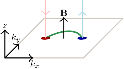
Figure 1: Schematic sketch of the half-space WSM geometry (defined by $z\geq 0$) in a homogeneous magnetic field $\mathbf{B}=B\hat{\mathbf{e}}_{z}$ perpendicular to the surface. The 3D WSM has two bulk Weyl nodes at momenta $\mathbf{k}=(\pm k_{0},0,0)^{T}$, corresponding to the red and blue circles for their surface projections. For $B=0$, the surface projections are connected by a Fermi-arc surface state (green curve). For $B\neq 0$, the low-energy bulk physics is dominated by the $n=0$ chiral LLs which have opposite chirality near different Weyl nodes (pink and light blue arrows show the respective propagation direction). Fermions incoming from a bulk chiral LL enter the arc at the surface. After sliding along the arc to the opposite Weyl node surface projection (in a semiclassical picture), they tunnel into the outgoing chiral LL [14].

Furthermore, in a WSM slab geometry (or in similar confined nanostructures), fermions in a chiral LL state move through the bulk and eventually tunnel into the opposite surface. There, they will traverse the corresponding opposite Fermi arc (in the semiclassical picture). In the simplest scenario, the fermion subsequently occupies the chiral LL state with opposite chirality and travels back to the initial Fermi arc state. This closed trajectory resembles an exotic cyclotron orbit, commonly referred to as “Weyl orbit”. Such orbits are predicted to cause unconventional quantum oscillations in the magnetoconductivity, with a strong dependence on the sample thickness [14, 15]. The initial prediction of Weyl orbits sparked excitement in the WSM community and led to a variety of subsequent theoretical proposals [16], including non-local transport experiments [17, 18, 19], the detection of chiral separation [20], and the chiral magnetic effect [21]. Weyl orbits are also important ingredients for an unconventional so-called 3D Quantum Hall Effect (QHE) [22, 23]. Both Shubnikov-de Haas oscillations due to Weyl orbits and the 3D QHE were thoroughly investigated in transport experiments for the Dirac semimetal Cd₃As₂ [24, 25, 26, 27, 28, 29], see also the review [16].

In a Dirac semimetal (DSM), Weyl nodes of opposite chirality share the same position in momentum space but are stabilized by space group symmetries of the crystal [3]. While the band structure is topologically trivial, pairs of Dirac cones can be connected by Fermi-arc surface states nevertheless. The semiclassical argument for the surface-bulk hybridization of Weyl orbits can be adapted to DSMs despite of the formally closed energy contour of surface states [14]. While clear experimental evidence for the predicted signatures has been collected for Cd₃As₂ [24, 25, 26, 27, 28, 29], their interpretation in terms of Weyl orbits remains debated [16]. In particular, thin films of Cd₃As₂ show an intricate dependence of the QHE on sample thickness [28, 30]. Moreover, energy quantization due to Weyl orbits is difficult to distinguish from the trivial size quantization of confined bulk states [31]. Similar arguments might also apply to the Weyl orbits reported in the non-centrosymmetric WSMs NbAs [32], TaAs [33] and WTe₂ [34]. So far, no Weyl orbits have been observed in magnetic WSMs with broken time-reversal symmetry [16]. However, recent experimental work on magnetic WSMs [35] and progress in quasiparticle interference experiments [36] render near-future advances in Weyl-orbit physics for this class of materials likely. These developments also motivated us to perform the present study.

A related exciting topic concerns twisted WSM interfaces [37, 38, 39, 40] and tunnel junctions [41]. Upon twisting interfaces with respect to each other, theory predicts a Fermi-arc reconstruction, implying the existence of “homo-chiral” Fermi arcs connecting Weyl nodes of equal chirality [38, 39]. In a magnetic field perpendicular to the interface, incoming electrons in a chiral LL may traverse the homo-chiral Fermi arc and tunnel back into bulk states on the other side of the junction, thereby achieving (almost) perfect transmission. Numerical transport simulations show good agreement with this semiclassical picture [41, 42, 43].

Adopting the half-space geometry, we here study the fate of Fermi-arc surface states in WSMs in a magnetic field. We construct a full quantum solution, going beyond semiclassics. To this end, we study a four-band low-energy continuum model for a magnetic WSM. While we find analytical solutions of the eigenproblem for the DSM limit of two degenerate Weyl nodes, we develop a numerical approach (with a controlled cut-off procedure) to obtain the eigenstates for the WSM scenario. We find that the eigenstates with lowest energy are composed of in- and out-going chiral zeroth-order LLs which are coupled by evanescent states localized near the surface. These are generated by all remaining higher-order LLs and cause a phase shift between in- and outgoing chiral LLs. In a slab geometry, this phase shift is experimentally observable through magnetoconductivity oscillations [14]. We compare our numerical results for the phase shift to semiclassical predictions by varying the energy $\varepsilon$ and a boundary parameter $\alpha$ encoding the arc curvature in the surface momentum plane. In addition, the energy derivative of the phase shift determines the Fermi-arc lifetime which is finite for $B\neq 0$. We show how the lifetime depends on key parameters such as $\alpha$, $\varepsilon,$ and $B$, and compare it to the semiclassical traversal time across the Fermi arc.

The remainder of this paper is structured as follows. In Sec. II we discuss the continuum WSM model employed here, derive boundary conditions for the half-space geometry, and present the surface state spectrum at zero magnetic field. We include the magnetic field in Sec. III and construct the eigenstates in the half-space geometry. In addition, we consider the limit of a DSM and obtain analytical solutions in several limiting cases. Subsequently, we derive the corresponding semiclassical predictions in Sec. IV and compare them with our quantum-mechanical results for the phase shift and for the Fermi-arc lifetime. The paper closes with concluding remarks in Sec. V. Details of our calculations can be found in several appendices. A derivation of $B=0$ Fermi-arc surface states is given in App. A. Their spin and current structure is discussed in App. B. We validate our numerical approach for finite magnetic fields in App. C, and discuss the Goos-Hänchen effect for the present setup in App. D. Throughout this paper, we use units with Fermi velocity $v_{F}=1$ and put $\hbar=1$.

II WSM in half space

In this section, we discuss the four-band WSM model employed in our study. The 3D model (in the absence of a magnetic field) is introduced in Sec. II.1. We then discuss the half-space geometry in terms of boundary conditions in Sec. II.2. The Fermi-arc surface states for $B=0$ are specified in Sec. II.3, see also App. A and App. B for further details.

II.1 Model

We study a four-band continuum WSM model which in 3D space, with conserved momentum $\mathbf{k}=(k_{x},k_{y},k_{z})^{T}$, is defined by the Hamiltonian [3]

$$H(\mathbf{k})=\mathbf{k}\cdot\bm{\sigma}\tau^{z}+k_{0}\sigma^{x}\tau^{0},$$ (1)

where $k_{0}\geq 0$ is the only free parameter. This parameter determines the distance between the Weyl nodes in momentum space. In Eq. (1), $\sigma^{\mu}$ and $\tau^{\mu}$ are Pauli matrices acting on effective spin and orbital degrees of freedoms, respectively, where $\mu=0$ refers to the identity and $\mu=x,y,z$ otherwise. We use $\bm{\sigma}=(\sigma^{x},\sigma^{y},\sigma^{z})$. While the limit $k_{0}=0$ describes a degenerate Dirac cone centered at $\mathbf{k}=\mathbf{0}$, i.e., a Dirac semimetal, the model exhibits two separated Weyl nodes at momenta $\mathbf{k}=\pm k_{0}\hat{\mathbf{e}}_{x}$ for $k_{0}>0$. Due to the block-diagonal structure of $H$, these Weyl nodes are decoupled. Their conserved chirality $\chi$ is associated with the orbital degree of freedom, namely the eigenvalues $\chi=\pm 1$ of $\tau^{z}$.

We note that adding a mass term $H^{\prime}=m\sigma^{0}\tau^{x}$ in Eq. (1) couples the Weyl nodes. However, for $m<k_{0}$, the Weyl nodes are thereby only shifted in momentum space and the low-energy description is not changed in an essential manner [3]. We thus put $m=0$ throughout this work. The two Weyl nodes are then fully decoupled in the bulk. This key simplification allows us to obtain explicit results in a finite magnetic field. Importantly, in our approach, the boundary conditions will couple both Weyl nodes. Furthermore, while Eq. (1) formally describes a type-I WSM with broken time-reversal symmetry and the minimum number of two Weyl nodes, we expect our arguments to apply to any WSM involving a pair of two isolated type-I Weyl nodes.

Below, we use the standard representation of Pauli matrices. States are written in the eigenbasis of $\sigma^{z}$ and $\tau^{z}$, i.e., $\ket{\chi}_{\bm{\tau}}$ for chirality $\chi=\pm 1$ and $\ket{\sigma}_{\bm{\sigma}}$ for spin $\sigma\in\{\uparrow,\downarrow\}$, with the spinor representations

$$\ket{+}_{\bm{\tau}} =\begin{pmatrix}1\\ 0\end{pmatrix}_{\bm{\tau}},\quad\ket{-}_{\bm{\tau}} =\begin{pmatrix}0\\ 1\end{pmatrix}_{\bm{\tau}},$$

$$\ket{\uparrow}_{\bm{\sigma}} =\begin{pmatrix}1\\ 0\end{pmatrix}_{\bm{\sigma}},\quad\ket{\downarrow}_{\bm{\sigma}} =\begin{pmatrix}0\\ 1\end{pmatrix}_{\bm{\sigma}}.$$ (2)

II.2 Half-space geometry and boundary conditions

We next proceed to the half-space geometry defined by $z\geq 0$, where we have a planar boundary at $z=0$ as illustrated in Fig. 1. Since the surface projections of the two Weyl nodes are separated, topological Fermi-arc surface states with an open energy contour connecting the projected nodes arise [3]. Before solving for the Fermi arcs, we first derive the general boundary condition from the constraint of Hermiticity of the Hamiltonian. For relativistic continuum models, such an approach typically allows for a few free parameters with physical implications on the surface state dispersion [44, 45, 46, 47].

For a derivation that is also valid in the presence of a finite magnetic field, we switch to real space by using the substitution $\mathbf{k}\rightarrow-i\nabla_{\mathbf{r}}$ in Eq. (1). Following standard arguments [44, 45, 46], we impose $\braket{\Psi_{1}}{H\Psi_{2}}-\braket{H\Psi_{1}}{\Psi_{2}}=0$ for arbitrary states $\Psi_{1}$ and $\Psi_{2}$ in the half-space geometry to infer a sufficient boundary condition,

$$\Psi_{1}^{\dagger}(\mathbf{r}_{\perp},z=0)j^{z}\Psi_{2}(\mathbf{r}_{\perp},z=0)=0.$$ (3)

Here, $\mathbf{r}_{\perp}=(x,y)^{T}$ is the in-plane position and $j^{z}=\sigma^{z}\tau^{z}$ is the $z$-component of the relativistic fermion particle current operator, $\mathbf{j}=\bm{\sigma}\tau^{z}$. Physically, Eq. (3) thus prohibits any local current flowing through the surface. This condition is ensured for states that satisfy boundary conditions of the form

$$M\Psi(\mathbf{r}_{\perp},z=0)=\Psi(\mathbf{r}_{\perp},z=0),$$ (4)

where $M$ is an operator with the properties

$$j^{z}M=-M^{\dagger}j^{z},\quad M^{2}=\mathbbm{1},$$ (5)

where $\mathbbm{1}=\sigma^{0}\tau^{0}$ is the identity. To parameterize all possible choices of $M$, we define the operators

$$M^{\bm{\tau}}_{\gamma}=\tau^{x}\cos{\gamma}+\tau^{y}\sin{\gamma},\quad M^{\bm{\sigma}}_{\delta}=\sigma^{x}\cos{\delta}+\sigma^{y}\sin{\delta},$$ (6)

in orbital and spin space, respectively. The most general Hermitian parameterization then involves four real parameters ($\alpha,\beta,\gamma,\delta)$,

$$M_{\alpha\beta\gamma\delta} = \cos{\alpha}\left(\sigma^{z}M^{\bm{\tau}}_{\gamma}\cos{\beta}+\sigma^{0}M^{\bm{\tau}}_{\gamma-\pi/2}\sin{\beta}\right)$$ (7)

$$+ \sin{\alpha}\left(\tau^{0}M^{\bm{\sigma}}_{\delta}\cos{\beta}+\tau^{z}M^{\bm{\sigma}}_{\delta-\pi/2}\sin{\beta}\right).$$

An equivalent parameterization was found in Refs. [48, 49] in the context of graphene monolayers. On general grounds, the number of free parameters in the boundary condition increases with the number of higher-energy bands in the model Hamiltonian [50, 51]. Consequently, the low-energy spectrum is not expected to change significantly when varying parameters within certain submanifolds of the full parameter space. Below, we do not exploit the complete parameter freedom in Eq. (7) but instead focus on a simple one-parameter boundary matrix $M$ allowing us to describe curved Fermi arcs.

II.3 Boundary spectrum at zero magnetic field

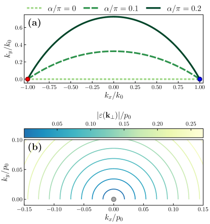
Figure 2: Surface-state spectrum of the four-band model (1) in a half space for $B=0$. (a) Zero-energy Fermi-arc contours in the $k_{x}$-$k_{y}$ plane as described by Eq. (9) for different boundary parameters $\alpha$, see also Fig. 1. (b) Surface-state contour-plot in the $k_{x}$-$k_{y}$ plane for a DSM ($k_{0}\to 0$) with $\alpha/\pi=0.1$ for different energies $\varepsilon(\mathbf{k}_{\perp})$ as indicated by the color bar, using a fixed scale $p_{0}$ as reference. The surface-state termination points result from the condition in Eq. (14).

Given the boundary condition (4) with the general parameterization (7), we next construct physical Fermi arc solutions for $B=0$, which are labeled by the conserved in-plane momentum $\mathbf{k}_{\perp}=(k_{x},k_{y})^{T}$. The simplest approach is to choose a block diagonal matrix $M$, e.g., the parametrization $M_{\frac{\pi}{2},0,0,\delta}$ in Eq. (7), which allows one to solve the problem for both Weyl nodes separately. The Fermi arc of a single Weyl node, which after a shift of $k_{x}$ is effectively described by $H_{\chi}=\chi\mathbf{k}\cdot\bm{\sigma}$, then becomes a semi-infinite line which terminates at the Weyl cone projection at an angle determined by the parameter $\delta$ [44, 45, 46]. The resulting surface-state spectrum of the four-band WSM model thus yields two semi-infinite arcs, in contrast to physical Fermi arcs which are open curves connecting both Weyl cone projections. Here, we will use boundary conditions which couple different Weyl nodes. This approach is especially convenient for $B\neq 0$.

To this end, we consider off-diagonal boundary matrices $M$ satisfying $[M,\sigma^{0}\tau^{z}]\neq 0$. The resulting boundary conditions couple the Weyl nodes at the surface. This picture is analogous to the one in Ref. [49], where armchair edges in graphene monolayers are modeled by boundary conditions that are non-diagonal in the valley degree of freedom. Below, we assume the boundary condition (4) with

$$M_{\alpha}=M_{\alpha,0,0,0}=\sigma^{z}\tau^{x}\cos{\alpha}+\sigma^{x}\tau^{0}\sin{\alpha}.$$ (8)

The parametrization (8) is a simple choice that allows us to construct physical Fermi arcs with a curvature in the surface momentum plane controlled by the single parameter $\alpha$. A curved arc is then symmetric under mid-point reflection, and a straight arc is found for $\alpha=0$ (mod $\pi$). As discussed in App. A, the particular choice of $M_{\alpha}$ in Eq. (8) is motivated by the observation that a straight arc requires $[M,j^{y}]=0$, where $j^{y}=\sigma^{y}\tau^{z}$ is the in-plane current operator along $\hat{\mathbf{e}}_{y}$. For a microscopic analysis of a specific material, one may instead employ boundary matrices $M$ containing more parameters (while still coupling both Weyl nodes), possibly guided by numerical calculations for lattice models. For simplicity, however, we focus on the one-parameter family of matrices in Eq. (8). In App. A, we derive the corresponding $B=0$ surface-state spectrum presented next.

We find that a physical Fermi-arc contour at energy $\varepsilon$ is given by $k_{y}=q_{\alpha}(\varepsilon,k_{x})$, where

$$q_{\alpha}(\varepsilon,k_{x})=\frac{(\varepsilon\sin{\alpha}-k_{0})(\varepsilon-k_{0}\sin{\alpha})-k_{x}^{2}\sin{\alpha}}{\cos{\alpha}\sqrt{(\varepsilon\sin{\alpha}-k_{0})^{2}-k_{x}^{2}\sin^{2}{\alpha}}}.$$ (9)

At zero energy, the contour terminates at both Weyl node surface projections ($k_{x}=\pm k_{0}$, $k_{y}=0$). The termination points $k_{x}=\pm k_{\varepsilon\alpha}$ for $\varepsilon\neq 0$ are implicitly given by

$$\varepsilon^{2}={\left(|k_{x}|-k_{0}\right)^{2}+[q_{\alpha}(\varepsilon,k_{x})]^{2}}.$$ (10)

Assuming $|\varepsilon|\ll k_{0}$ and expanding Eq. (9) to lowest order in $\varepsilon/k_{0}$, we estimate

$$k_{\varepsilon\alpha}=k_{0}-\frac{4\varepsilon\sin{\alpha}}{3-\cos{(2\alpha)}}.$$ (11)

Moreover, we find the low-energy dispersion relation

$$\varepsilon(\mathbf{k}_{\perp}) \simeq\frac{k_{0}^{2}-k_{x}^{2}\sin^{2}{\alpha}}{k_{0}^{2}-k_{x}^{2}\sin^{4}{\alpha}}\bigg{(}\frac{k_{0}^{2}-k_{x}^{2}}{k_{0}}\sin{\alpha}$$

$$-\sqrt{k_{0}^{2}-k_{x}^{2}\sin^{2}{\alpha}}\,\frac{k_{y}}{k_{0}}\cos{\alpha}\bigg{)}.$$ (12)

For $\alpha=0$, the above expressions are exact and describe a straight arc with $\varepsilon(\mathbf{k}_{\perp})=-k_{y}$. For $\alpha\neq 0$, the arc is curved in the surface momentum plane as illustrated in Fig. 2(a). We note that the Fermi arc for $\alpha\to\pi-\alpha$ with the same energy $\varepsilon$ follows by reflection with respect to the $k_{x}$-axis. In effect, this transformation yields the Fermi arc for the same boundary condition but in the opposite half-space $z\leq 0$, see App. A. We briefly discuss the in-plane spin and current densities associated with Fermi-arc states in App. B.

Next, we turn to the limit $k_{0}\to 0$ describing the low-energy theory of a DSM with a single degenerate cone. While the band structure is now topogically trivial, surface states may nonetheless exist. Such states become important for $B\neq 0$, see Sec. IV. Deferring technical details to App. A, we find topologically trivial surface states with the dispersion relation

$$\varepsilon_{\pm}(\mathbf{k}_{\perp})=\pm\sqrt{k_{x}^{2}+k^{2}_{y}\cos^{2}{\alpha}},$$ (13)

which only exist if the condition

$$k_{y}\sin{\alpha}>0$$ (14)

is satisfied. In particular, there neither are surface state solutions for $\alpha=0$ (mod $\pi$), corresponding to a straight arc for finite $k_{0}$, nor for $\varepsilon=0$. Below, we focus on those two cases for analytical results. For finite $\alpha$ or $\varepsilon$, however, surface states emerge which form open energy contours. These contours shrink with decreasing energy, see Fig. 2(b).

III Half space in a magnetic field

In this section, we include the magnetic field $\mathbf{B}=B\hat{\mathbf{e}}_{z}$ with $B>0$ and study the WSM model in Sec. II for the half-space geometry using the boundary condition (4) defined by the matrix $M_{\alpha}$ in Eq. (8). The parameter $\alpha$ determines the curvature of the $B=0$ Fermi arc solutions. In Sec. III.1, we briefly review the eigenstates for the infinite 3D problem. In Sec. III.2, we then turn to the half-space problem and construct the low-energy quantum-mechanical eigenstates.

III.1 Landau quantization

We start with the free-space WSM model and we incorporate the homogeneous magnetic field $\mathbf{B}$ by minimal coupling, $\mathbf{k}\to-i\nabla_{\mathbf{r}}+\frac{e}{c}\mathbf{A}$, where $e>0$ is the (absolute value of the) electron charge and $c$ is the speed of light. For convenience, we choose the Landau gauge, $\mathbf{A}=-By\hat{\mathbf{e}}_{x}$, where Eq. (1) gives

$$H=-i\nabla_{\mathbf{r}}\cdot\bm{\sigma}\tau^{z}-\frac{y}{\ell_{B}^{2}}\sigma^{x}\tau^{z}+k_{0}\sigma^{x}\tau^{0}=\begin{pmatrix}H_{+}&0\\ 0&H_{-}\end{pmatrix}_{\bm{\tau}}$$ (15)

with the magnetic length $\ell_{B}=\sqrt{c/eB}$. Note that the chosen gauge retains translation invariance along $\hat{\mathbf{e}}_{x}$. The momentum component $k_{x}$ therefore remains a good quantum number.

When solving for LL solutions, it is convenient to consider the Weyl nodes separately. A single Weyl node with chirality $\chi=\pm 1$ and momentum $\mathbf{k}=-\chi k_{0}\hat{\mathbf{e}}_{x}$ is described by the Hamiltonian $H_{\chi}$ in spin space using the block diagonal form in Eq. (15). For given $\chi$ and $k_{x}$, we define the bosonic ladder operator

$$a^{\dagger}_{\chi}=\frac{\ell_{B}}{\sqrt{2}}\left(\frac{y}{\ell_{B}^{2}}-k_{x}-\chi k_{0}-\partial_{y}\right),$$ (16)

with the commutator $[a_{\chi},a_{\chi}^{\dagger}]=1$. The transverse part of $H_{\chi}=-i\chi\partial_{z}\sigma^{z}+H^{\perp}_{\chi}$ is thereby written as

$$H_{\chi}^{\perp}=-\frac{\chi}{\sqrt{2}\ell_{B}}\left[\left(a_{\chi}+a_{\chi}^{\dagger}\right)\sigma^{x}+i\left(a_{\chi}-a_{\chi}^{\dagger}\right)\sigma^{y}\right].$$ (17)

In the infinite 3D system (without boundary), the momentum component $k_{z}$ is also conserved. It is then straightforward to obtain the well-known relativistic LLs $\varepsilon^{\chi}_{nk_{z}}$ labeled by non-negative integer $n\in\mathbbm{N}_{0}$ [3],

$$\varepsilon^{\chi}_{0,k_{z}}=-\chi k_{z},\quad\varepsilon^{\chi}_{\pm,n>0,k_{z}}=\pm\chi\sqrt{\frac{2n}{\ell_{B}^{2}}+k_{z}^{2}}.$$ (18)

Here, $\varepsilon^{\chi}_{0,k_{z}}$ is the dispersion of the gapless chiral LL, while $n>0$ correspond to higher-order gapped LL states. Eigenstates are expressed in terms of harmonic oscillator eigenfunctions,

$$\varphi_{n}(y)=\frac{H_{n}(y/\ell_{B})}{\sqrt{2^{n}n!\sqrt{\pi}\,\ell_{B}}}\,{\mathrm{e}}^{-\frac{1}{2}{(y/\ell_{B})^{2}}},$$ (19)

where $H_{n}$ is the $n$th-order Hermite polynomial. Writing $a_{\chi}^{\dagger}a_{\chi}\varphi_{n}^{\chi}=n\varphi_{n}^{\chi}$, the wave functions

$$\varphi_{n}^{\chi}(y)=\varphi_{n}(y-\ell_{B}^{2}k_{x}-\chi\ell_{B}^{2}k_{0})$$ (20)

incorporate a shift with respect to the Weyl node position. In anticipation of the half-space geometry, we label the solutions $\ket{\psi^{\chi}_{n\varepsilon}}$ of $H_{\chi}\ket{\psi^{\chi}_{n\varepsilon}}=\varepsilon\ket{\psi^{\chi}_{n\varepsilon}}$ in terms of energy $\varepsilon$ instead of $k_{z}$. The chiral LL with $n=0$ is then described by

$$\psi^{\chi}_{0,\varepsilon}(y,z)=\frac{\mathrm{e}^{-i\chi\varepsilon z}}{\sqrt{2\pi}}\begin{pmatrix}0\\ \varphi_{0}^{\chi}(y)\end{pmatrix}_{\bm{\sigma}}.$$ (21)

Since $k_{x}$ is conserved, we keep plane-wave factors $e^{ik_{x}x}$ and the $k_{x}$-dependence of observables implicit below. Similar expressions as Eq. (21) hold for the wave functions of $n>0$ bulk LLs [5].

In the following, we focus on the ultra-quantum regime, $|\varepsilon|<{\sqrt{2}}/{\ell_{B}}$. While $n>0$ bulk LLs do not exist in this regime, it is possible to construct evanescent solutions in the half-space geometry by solving the eigenproblem for imaginary momentum $k_{z}=i\kappa$ with $\kappa=\kappa_{n\varepsilon}>0$. The evanescent solution for $n>0$ is given by

$$\psi^{\chi}_{n\varepsilon}(y,z)=\sqrt{\kappa_{n\varepsilon}}\,{\mathrm{e}^{-\kappa_{n\varepsilon}z}}\begin{pmatrix}\chi\mathrm{e}^{i\chi\gamma_{n\varepsilon}}\varphi_{n-1}^{\chi}(y)\\ \varphi_{n}^{\chi}(y)\end{pmatrix}_{\bm{\sigma}},$$ (22)

with the inverse penetration length

$$\kappa_{n\varepsilon}=\sqrt{2n/\ell_{B}^{2}-\varepsilon^{2}}$$ (23)

and the phase $\gamma_{n\varepsilon}$ defined by

$$\mathrm{e}^{i\gamma_{n\varepsilon}}=-\frac{\ell_{B}}{\sqrt{2n}}(\varepsilon+i\kappa_{n\varepsilon}).$$ (24)

One can rationalize the appearance of this complex phase factor by noticing that evanescent solutions do not carry any current along $\hat{\mathbf{e}}_{z}$, i.e., $\braket{\psi^{\chi}_{n\varepsilon}}{\sigma^{z}}{\psi^{\chi}_{n\varepsilon}}=0$ for $n>0$.

III.2 Half-space geometry

III.2.1 Coupling of Weyl nodes at the boundary

We now proceed to the half-space geometry $z\geq 0$ sketched in Fig. 1, see Sec. II for the $B=0$ case. We first rewrite the boundary condition (4) with the matrix $M_{\alpha}$ in Eq. (8) as

$$\mathbbm{V}_{\alpha}(z)\Psi(\mathbf{r})=0,\quad\mathbbm{V}_{\alpha}(z)=\delta(z)\left(\mathbbm{1}-M_{\alpha}\right).$$ (25)

Our Ansatz for solving Eq. (25) is a superposition of all eigenstates of $H$ in Eq. (15) with given $\varepsilon$ and $k_{x}$. We focus on the ultra-quantum regime $|\varepsilon|<\sqrt{2}/\ell_{B}$, where $n>0$ LL states only contribute through evanescent-state solutions in Eq. (22). Combining the results of Eqs. (21) and (22) gives

$$\ket{\Psi_{\varepsilon}}=\sum_{\chi=\pm}\sum_{n\geq 0}c^{\chi}_{n\varepsilon}\ket{\psi^{\chi}_{n\varepsilon}}_{\bm{\sigma}}\ket{\chi}_{\bm{\tau}},$$ (26)

where the $c^{\chi}_{n\varepsilon}$ are complex coefficients which have to be determined. Equation (25) states that $\ket{\Psi_{\varepsilon}}$ is element of the kernel of $\mathbbm{V}_{\alpha}$. Matrix elements of this operator, restricted to the subspace with fixed energy $\varepsilon$, are of the form

$$\left[V_{\alpha}(\varepsilon)\right]^{\chi,\chi^{\prime}}_{n,n^{\prime}}=_{\bm{\tau}}\bra{\chi}\,_{\bm{\sigma}}\bra{\psi_{n\varepsilon}^{\chi}}\mathbbm{V}_{\alpha}(z)\ket{\psi^{\chi^{\prime}}_{n^{\prime}\varepsilon}}_{\bm{\sigma}}\ket{\chi^{\prime}}_{\bm{\tau}}.$$ (27)

For convenience, we rescale them as

$$[\hat{V}_{\alpha}(\varepsilon)]^{\chi,\chi^{\prime}}_{n,n^{\prime}}=\left(\kappa_{n\varepsilon}\kappa_{n^{\prime}\varepsilon}\right)^{-\frac{1}{2}}\left[V_{\alpha}(\varepsilon)\right]^{\chi,\chi^{\prime}}_{n,n^{\prime}}$$ (28)

with $\kappa_{0,\varepsilon}=1/2\pi$. Matrix elements between a chiral $n=0$ LL and $n\geq 0$ LLs with equal chirality $\chi$ are given by

$$[\hat{V}_{\alpha}(\varepsilon)]^{\chi,\chi}_{0,n}=\delta_{n,0}-\chi\mathrm{e}^{i\chi\gamma_{n\varepsilon}}\delta_{n,1}\sin{\alpha},$$ (29)

while for $n,n^{\prime}>0$, we find

$$[\hat{V}_{\alpha}(\varepsilon)]^{\chi,\chi}_{n,n^{\prime}} =2\delta_{n,n^{\prime}}-\chi\mathrm{e}^{i\chi\gamma_{n+1,\varepsilon}}\delta_{n,n^{\prime}-1}\sin{\alpha}$$

$$-\chi\mathrm{e}^{-i\chi\gamma_{n\varepsilon}}\delta_{n,n^{\prime}+1}\sin{\alpha}.$$ (30)

Matrix elements for opposite chiralities resemble the coupling of Weyl nodes in terms of the boundary condition. For $n\geq 0$, we obtain

$$[\hat{V}_{\alpha}(\varepsilon)]^{\chi,-\chi}_{0,n}=\braket{\varphi^{\chi}_{0}}{\varphi^{-\chi}_{n}}\cos{\alpha}.$$ (31)

Finally, for $n,n^{\prime}>0$, we find

$$[\hat{V}_{\alpha}(\varepsilon)]^{\chi,-\chi}_{nn^{\prime}} =\cos{\alpha}\left(\mathrm{e}^{-i\chi(\gamma_{n\varepsilon}+\gamma_{n^{\prime}\varepsilon})}\braket{\varphi^{\chi}_{n-1}}{\varphi^{-\chi}_{n^{\prime}-1}}\right.$$ (32)

$$\left.+\braket{\varphi^{\chi}_{n}}{\varphi^{-\chi}_{n^{\prime}}}\right).$$

The overlap $\braket{\varphi^{\chi}_{n}}{\varphi^{-\chi}_{m}}$ involves shifted harmonic oscillator eigenfunctions associated with different Weyl nodes. Performing the integration for $n\geq m$ yields [52]

$$\braket{\varphi^{-}_{n}}{\varphi^{+}_{m}} =\int dy\,\varphi_{n}(y-l_{B}^{2}k_{0})\varphi_{m}(y+l_{B}^{2}k_{0})$$ (33)

$$=\sqrt{2^{n-m}\frac{m!}{n!}}\lambda_{B}^{n-m}L_{m}^{n-m}(2\lambda_{B}^{2})\mathrm{e}^{-\lambda_{B}^{2}},$$

with the dimensionless quantity

$$\lambda_{B}=k_{0}\ell_{B},$$ (34)

which measures the decoupling of the Weyl nodes by the magnetic field. In Eq. (33), $L^{m}_{n}$ is a generalized $n$th-order Laguerre polynomial. In App. C, we describe a recursion relation allowing for the numerically efficient computation of the overlaps in Eq. (33). The remaining terms follow from the relation $\braket{\varphi^{+}_{n}}{\varphi^{-}_{m}}=(-1)^{n-m}\braket{\varphi^{-}_{n}}{\varphi^{+}_{m}}$. We note that the overlaps allow for a perturbative treatment in the large-field limit $\lambda_{B}\ll 1$. Let us also mention in passing that similar expressions appear when computing matrix elements of the bulk mass term $m\sigma^{0}\tau^{x}$. In that case, the coupling opens a gap in the dispersion of the chiral LLs of the order of $\braket{\varphi_{0}^{+}}{\varphi_{0}^{-}}=\mathrm{e}^{-\lambda_{B}^{2}}$. This result is consistent with the WKB approximation for a two-band WSM model with two Weyl nodes [53, 54].

In any case, convergence of the overlaps $\lim_{n\to\infty}\braket{\varphi^{+}_{n}}{\varphi^{-}_{m}}=0$ is ensured for arbitrary $\lambda_{B}$. This fact justifies the introduction of a cut-off $N$ for the LL index, $n<N$, reducing the numerical solution of the boundary problem to a linear algebra problem,

$$V_{\alpha}(\varepsilon){\mathbf{c}}_{\varepsilon}=\mathbf{0},$$ (35)

where $V_{\alpha}(\varepsilon)$ is a $2N\times 2N$ matrix formed by the matrix elements (27) of the lowest $N$ LLs and $\mathbf{c}_{\varepsilon}$ is a vector containing the corresponding coefficients $c^{\chi}_{n\varepsilon}$. The numerical solution of Eq. (35) then determines the eigenstates of the WSM in the half-space geometry for $B\neq 0$. In App. C, we carefully verify the controlled nature of the above cut-off procedure and the accuracy of the boundary condition.

Due to current conservation, coefficients with the same $(n,\varepsilon,k_{x})$ but different chiralities have the same absolute value, $|c_{n\varepsilon}^{+}|=|c_{n\varepsilon}^{-}|$. In particular, we are interested in the phase shift $\theta_{\alpha}(\varepsilon)$ between in- and outgoing chiral $n=0$ Landau states,

$${c_{0,\varepsilon}^{-}}=\mathrm{e}^{i\theta_{\alpha}(\varepsilon)}{c_{0,\varepsilon}^{+}}.$$ (36)

We note that all phases below are defined only modulo $2\pi$. The phase shift $\theta_{\alpha}(\varepsilon)$ depends on the global phase choices for the basis states in Eq. (26). While for a fixed phase choice, $\theta_{\alpha}(\varepsilon)$ is formally gauge invariant, observable quantities must also be independent of the phase choice. Full gauge invariance is ensured below by only considering phase shift differences, $\Phi=\theta_{\alpha^{\prime}}(\varepsilon^{\prime})-\theta_{\alpha}(\varepsilon)$. When combined with the corresponding phase shift on the opposite surface in a slab geometry, one can infer the magnetoconductivity oscillation period of the corresponding Weyl orbit from Eq. (36) [14]. We compare our quantum-mechanical results for $\Phi$ to semiclassical estimates in Sec. IV.

We note that for a straight arc at zero energy, $\alpha=0$ (mod 2$\pi$) and $\varepsilon=0$, with the basis choice in Eq. (26), one finds

$$\theta_{\alpha=0}(\varepsilon=0)=\pi.$$ (37)

We verify Eq. (37) by evaluating the boundary condition at $y=\ell_{B}^{2}k_{x}$, where $\varphi^{+}_{n}(\ell_{B}^{2}k_{x})=(-1)^{n}\varphi^{-}_{n}(\ell_{B}^{2}k_{x})$. By virtue of $|c^{+}_{n\varepsilon}|=|c^{-}_{n\varepsilon}|$ and the boundary condition, we then arrive at $c_{n,0}^{+}=(-1)^{n+1}c_{n,0}^{-}$, and thus at Eq. (37).

Since eigenstates in the half-space geometry can be written in the form (26), a nontrivial $y$-dependence arises since the separation between Weyl nodes in momentum space appears in the argument of Eq. (20). As shown in App. D, this observation implies that an electron incident on the surface undergoes a shift (assuming $\varepsilon>0$)

$$\delta y=-2\ell_{B}^{2}k_{0}$$ (38)

in the $y$-direction. This effect can be interpreted semiclassically in terms of chiral transport associated to Fermi arcs, see App. B.

III.2.2 Dirac semimetal

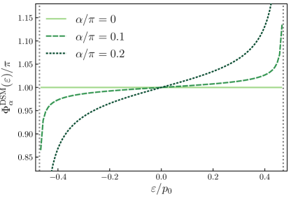
Figure 3: Gauge invariant phase shift $\Phi^{\rm DSM}_{\alpha}(\varepsilon)$ vs energy $\varepsilon$ for chiral LLs in a DSM ($k_{0}\to 0$) for several values of $\alpha$, see Eq. (43). The shown results were obtained by a numerical solution of the quantum-mechanical problem. We use $p_{0}\ell_{B}=3$ with a reference scale $p_{0}$, where $\varepsilon$ is shown in units of $p_{0}$ (with $v_{F}=1$). The ultra-quantum regime $|\varepsilon|<\sqrt{2}/\ell_{B}$ is indicated by vertical dotted lines.

In order to identify contributions to the phase shift (36) picked up by fermions traversing the Fermi arc in Sec. IV, let us briefly consider the analogous problem in the DSM limit $k_{0}\to 0$. The corresponding linear system follows from Eq. (35) by inserting diagonal overlaps $\braket{\varphi^{-}_{n}}{\varphi^{+}_{m}}=\delta_{nm}$ in Eqs. (31) and (32). For analytical results, we focus on cases without topologically trivial surface states for $B=0$, i.e., we consider either $\alpha=0$ (mod $\pi$) or $\varepsilon=0$.

First, for $\alpha=0$ (mod $2\pi$), it is straightforward to show that the boundary condition (4) with $M_{0}=\sigma^{z}\tau^{x}$ is satisfied by antisymmetric superpositions of chiral LLs,

$$\ket{\Psi_{\varepsilon}}=\frac{1}{\sqrt{2}}\left(\ket{\psi^{+}_{0,\varepsilon}}_{\bm{\sigma}}\ket{+}_{\bm{\tau}}-\ket{\psi^{-}_{0,\varepsilon}}_{\bm{\sigma}}\ket{-}_{\bm{\tau}}\right).$$ (39)

With the above basis choice, we then obtain the phase shift $\theta_{\alpha=0}(\varepsilon)=\theta^{\rm DSM}_{\alpha=0}(\varepsilon)=\pi$ for arbitrary $\varepsilon$. Similarly, one finds $\theta^{\rm DSM}_{\pi}(\varepsilon)=0$.

Second, for $\varepsilon=0$ but arbitrary $\alpha$, by using $\gamma_{n,\varepsilon=0}=-\pi/2$, the linear system (35), expressed in terms of the rescaled coefficients $\hat{c}^{\chi}_{n}=\sqrt{\kappa_{n,\varepsilon=0}}{c}^{\chi}_{n,\varepsilon=0}$, simplifies to

$$0 =\hat{c}^{\chi}_{0}+\cos{\alpha}\,\hat{c}^{-\chi}_{0}+i\sin{\alpha}\,\hat{c}^{\chi}_{1},$$

$$0 =2\hat{c}^{\chi}_{n}-i\sin{\alpha}\left(\hat{c}^{\chi}_{n+1}-\hat{c}^{\chi}_{n-1}\right).$$ (40)

The physical solution of the recursion relation is (we here assume $\cos\alpha>0$)

$$\hat{c}^{+}_{0}=-\hat{c}^{-}_{0},\quad\hat{c}^{\chi}_{n}=\left(i\tan{\frac{\alpha}{2}}\right)^{n}\hat{c}^{\chi}_{0}.$$ (41)

Without need for a cut-off $N$ and up to normalization, we thereby arrive at the exact solution

$$\ket{\Psi_{\varepsilon=0}}\propto\sum_{\chi=\pm}\chi\sum_{n\geq 0}\frac{1}{\sqrt{\kappa_{n,0}}}\left(i\tan{\frac{\alpha}{2}}\right)^{n}\ket{\psi^{\chi}_{n,0}}_{\bm{\sigma}}\ket{\chi}_{\bm{\tau}}.$$ (42)

Clearly, the phase shift is again given by $\theta^{\rm DSM}_{\alpha}(\varepsilon=0)=\pi$. Remarkably, the superposition state (42) involves evanescent contributions even though no surface state exists for $\varepsilon=0$ with $B=0$ and $k_{0}=0$, see Eqs. (13) and (14). An analogous calculation leads to $\theta^{\rm DSM}_{\pi-\alpha}(0)=0$.

For finite $\alpha$ and finite $\varepsilon$, we solve the problem numerically as described above. As shown in Fig. 3, we then find a finite gauge invariant phase shift, which we define as

$$\Phi^{\rm DSM}_{\alpha}(\varepsilon)=\theta^{\rm DSM}_{\alpha}(\varepsilon)-\theta^{\rm DSM}_{\pi}(\varepsilon).$$ (43)

(The reason for substracting the phase for $\alpha=\pi$ is explained in Sec. IV.) For small $\alpha$ and $\varepsilon$, this phase shift turns out to be small compared to the corresponding phase shifts in WSMs, see Sec. IV. Since the main focus of this work in on the WSM case, we leave a detailed (semiclassical) discussion of phase shifts in DSMs to future studies.

IV Results and comparison to semiclassics

The semiclassical theory for Fermi arcs in WSMs in a magnetic field is well established [14, 15]. According to this standard picture, fermions in the chiral LL tunnel into a Fermi-arc state upon reaching the surface. The Lorentz force then drives the fermion along the arc to the other Weyl cone projection of opposite chirality, where it can tunnel back into the bulk and thereby escape from the surface. In a slab geometry, this process is repeated on the opposite surface, and the semiclassical trajectory forms a closed Weyl orbit which can be described using semiclassical quantization [14, 15].

In the half-space geometry, the semiclassical trajectory is open and no quantization is expected. This enables us to disentangle bulk and surface contributions. The latter are determined by the semiclassical equations of motion for an electron moving along the Fermi arc (with $\mathbf{k}=\mathbf{k}_{\perp}$) [55, 14],

$$\dot{\mathbf{k}}=-\frac{1}{\ell_{B}^{2}}\mathbf{v}_{\mathbf{k}}\times\hat{\mathbf{e}}_{z},\quad\dot{\mathbf{r}}=\mathbf{v}_{\mathbf{k}}=\nabla_{\mathbf{k}}\varepsilon(\mathbf{k}),$$ (44)

where $\mathbf{v}_{\mathbf{k}}$ is the group velocity in the $x$-$y$ plane and $\varepsilon=\varepsilon(\mathbf{k})$ is the arc dispersion relation. Here, we neglect the anomalous velocity contribution due to the Berry curvature of generic Fermi-arc states [55, 56]. This approximation can be justified by noting that the Berry curvature vanishes for a straight arc and we consider the small-$\alpha$ case below. As a consequence, $\dot{\mathbf{k}}$ is tangential to the energy contour.

IV.1 Phase shifts accumulated along Fermi-arc curves

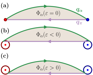
Figure 4: Schematic illustration of closed trajectories in the surface momentum plane used for the semiclassical calculation of the gauge invariant phase $\Phi_{\alpha}(\varepsilon)$ in Eq. (47). A curved Fermi arc (green) with $0<\cos\alpha<1$ is joined with a straight Fermi arc (purple) for $\alpha=\pi$. Arrows indicate the direction of $\dot{\mathbf{k}}$ as described by Eq. (44). We show the corresponding closed trajectories (a) for zero energy ($\varepsilon=0$), (b) for $\varepsilon<0$, and (c) for $\varepsilon>0$. For $\varepsilon\neq 0$, the curved arc termination points, $(k_{x},k_{y})=(\pm k_{\varepsilon\alpha},q_{\alpha}(\varepsilon,k_{\varepsilon\alpha}))$, differ from the Weyl node projections $(\pm k_{0},0)$ corresponding to the circle centers in panels (b) and (c). To match the arc termination points of the curved arc and the straight reference arc, we employ a rescaling $k_{0}\to k_{\varepsilon\alpha}$ for the straight arc case. For details, see main text.

We first consider the phase shift $\theta_{\alpha}(\varepsilon)$ between the chiral LLs in Eq. (36) for a curved Fermi arc with $0<\cos\alpha<1$. In a semiclassical picture, this phase shift can be estimated by a phase-space integral of the schematic form

$$\theta_{\alpha}(\varepsilon)=\int d\mathbf{r}\cdot\left(\mathbf{k}-\frac{e}{c}\mathbf{A}\right).$$ (45)

For gauge invariant phases, we need closed trajectories in real space. This issue is closely related to the fact that the quantum-mechanical phase shift $\theta_{\alpha}(\varepsilon)$ discussed in Sec. III.2 becomes gauge invariant only after switching to a phase shift difference. For the semiclassical counterpart, we resolve this issue by introducing a straight reference arc which reconnects the termination points of the curved Fermi arc. We thereby obtain a closed trajectory in the surface momentum plane, see Fig. 4, where the phase $\Phi_{\alpha}(\varepsilon)$ accumulated along the trajectory is gauge invariant. To ensure that also the corresponding real-space trajectory is closed, we recall that the transformation $\alpha\to\alpha+\pi$ inverts the sign of the group velocity component $v_{y}$, and thus of $\dot{k}_{x}$, see Eq. (44). In effect, this allows for a closed motion in the surface momentum plane, where the straight reference arc is chosen to have $\alpha=\pi$.

The above procedure is straightforwardly implemented at zero energy ($\varepsilon=0$), where the arc termination points are at $(k_{x},k_{y})=(\pm k_{0},0)$ for all values of $\alpha$, see Fig. 4(a). On the quantum level, we then consider the phase shift difference $\Phi_{\alpha}(\varepsilon=0)=\theta_{\alpha}(0)-\theta_{\pi}(0)$, where $\theta_{\pi}(0)=\pi$, see Eq. (37).

The situation becomes more intricate for $\varepsilon\neq 0$ since now the curved arc termination points, $(k_{x},k_{y})=(\pm k_{\varepsilon\alpha},q_{\alpha}(\varepsilon,k_{\varepsilon\alpha}))$, differ from the corresponding Weyl node projections at $(\pm k_{0},0)$. (We recall that $k_{\varepsilon\alpha}$ follows by solving Eq. (10), see also the estimate in Eq. (II.3). Moreover, the function $q_{\alpha}(\varepsilon,k_{x})$ parameterizing the Fermi-arc contour at energy $\varepsilon$ has been defined in Eq. (9).) For the straight reference arc, we therefore consider a system with rescaled Weyl node separation, $k_{0}\to k_{\varepsilon\alpha}$, at energy $\varepsilon\to\bar{\varepsilon}=q_{\alpha}(\varepsilon,k_{\varepsilon\alpha})$. The arc termination points for the straight reference arc are then located at $(\pm k_{\varepsilon\alpha},\bar{\varepsilon})$ and match the termination points of the curved arc, see Fig. 4(b,c). We note that the energy of the reference arc differs from the energy of the curved Fermi arc. We can ensure only in this manner that both arc contours connect at their termination points and enclose a finite area in momentum space. No need for such a construction would arise for Weyl orbits in a slab geometry, where tunneling processes via bulk states take care of the corresponding momentum shifts between arc termination points on opposite surfaces. The advantage of our approach is that bulk states do not appear explicitly in the semiclassical calculation.

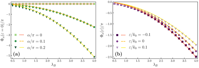
Figure 5: Comparison of quantum-mechanical results and semiclassical estimates for the gauge invariant Fermi-arc surface-state phase shift $\Phi_{\alpha}(\varepsilon)$, see Eqs. (46) and (IV.1), respectively. The phase $\Phi_{\alpha}(\varepsilon)$ is shown as function of the parameter $\lambda_{B}=k_{0}\ell_{B}$ and gives the phase accumulated along the closed trajectories in surface-momentum space illustrated in Fig. 4. Symbols show the numerical solution of the quantum problem, and curves show the corresponding semiclassical predictions. Integer multiples of $2\pi$ have been added to obtain smooth curves. (a) Zero-energy case ($\varepsilon=0$) for different $\alpha$. (a) Case $\alpha/\pi=0.1$ for different energies $\varepsilon$.

On the quantum level, we then define the gauge invariant phase shift difference as

$$\Phi_{\alpha}(\varepsilon)=\theta_{\alpha}(\varepsilon)-\bar{\theta}_{\pi}\left(-q_{\alpha}(\varepsilon,k_{\varepsilon\alpha})\right)-\Phi^{\rm DSM}_{\alpha}(\varepsilon),$$ (46)

where $\bar{\theta}_{\pi}$ follows by solving the linear system (35) with the rescaled parameter $\lambda_{B}\to\bar{\lambda}_{B}=\ell_{B}^{2}k_{\varepsilon\alpha}$. For a comparison to semiclassical results, in Eq. (46), we also subtract the phase shift difference $\Phi_{\alpha}^{\rm DSM}(\varepsilon)$, see Eq. (43), for the corresponding DSM case as shown in Fig. 3.

On the semiclassical level, the above gauge invariant phase shift takes the form

$$\Phi_{\alpha}(\varepsilon) =\oint d\mathbf{r}\cdot\left(\mathbf{k}-\frac{e}{c}\mathbf{A}\right)$$

$$=-\ell_{B}^{2}\int_{-k_{\varepsilon\alpha}}^{k_{\varepsilon\alpha}}dk_{x}\,\left(q_{\alpha}(\varepsilon,k_{x})-q_{\alpha}(\varepsilon,k_{\varepsilon\alpha})\right),$$ (47)

As illustrated in Fig. 4, the phase $\Phi_{\alpha}(\varepsilon)$ in Eq. (47) corresponds to the momentum-space area enclosed by the curved Fermi arc and the straight reference arc. Assuming $|\varepsilon|\ll k_{0}$, we find

$$\Phi_{\alpha}(\varepsilon) \simeq\ell_{B}^{2}k_{0}^{2}\frac{2\alpha\cot{(2\alpha)}-1}{\sin{\alpha}}$$

$$+2\ell_{B}^{2}\varepsilon k_{0}\left(1+\alpha\tan{\alpha}-\frac{2\cos^{2}{\alpha}}{3-\cos{(2\alpha)}}\right).$$ (48)

In Fig. 5, for small energies $\varepsilon$, we compare quantum-mechanical results for $\Phi_{\alpha}(\varepsilon)$ obtained numerically from Eq. (46) to the corresponding semiclassical predictions in Eq. (IV.1). We find quantitative agreement both for different arc curvatures, see Fig. 5(a), and for different energies, see Fig. 5(b). It is worth noting that the semiclassical description remains accurate even for large magnetic fields with $\lambda_{B}<1$.

IV.2 Fermi-arc lifetime and semiclassical traversal time

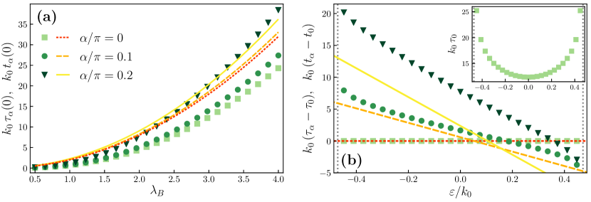
Figure 6: Quantum-mechanical results for the Fermi-arc lifetime $\tau_{\alpha}(\varepsilon)$ [symbols] and for the semiclassical arc traversal time $t_{\alpha}(\varepsilon)$ [curves], see Eqs. (49) and (51), respectively, for several values of $\alpha$ and given in units of $k_{0}^{-1}$. (a) Dependence of $\tau_{\alpha}$ and $t_{\alpha}$ on $\lambda_{B}$ for $\varepsilon=0$. (b) $\tau_{\alpha}-\tau_{0}$ vs $\varepsilon$ in the ultra-quantum regime (delimited by vertical dotted lines) for $\lambda_{B}=3$. Different symbols are for different $\alpha$ as in panel (a). We also show the corresponding semiclassical traversal time differences $t_{\alpha}-t_{0}$. The inset shows the straight-arc lifetime $\tau_{\alpha=0}$ vs $\varepsilon$, again for $\lambda_{B}=3$.

As discussed in Sec. I, one expects that Fermi-arc surface states acquire a finite lifetime $\tau_{\alpha}(\varepsilon)$ in a finite magnetic field $B\neq 0$. The lifetime describes the time scale for escaping into the bulk via the chiral LLs and follows from the general relation [57, 58]

$$\tau_{\alpha}(\varepsilon)=\frac{d\theta_{\alpha}(\varepsilon)}{d\varepsilon}.$$ (49)

We note that this phase shift includes DSM contributions. Being a physical observable, Eq. (49) is gauge invariant. We compute Eq. (49) numerically using the quantum-mechanical approach detailed in Sec. III.

On the semiclassical level, we define another time scale, namely the traversal time $t_{\alpha}(\varepsilon)$. This is the time required to traverse the Fermi arc from one termination point to the other. Since the lifetime is due to the escape of Fermi-arc electrons into the bulk at the arc termination points, one expects that $t_{\alpha}(\varepsilon)$ is of the same order as $\tau_{\alpha}(\varepsilon)$. We will therefore compare these two time scales below. The semiclassical traversal time follows with Eq. (9) in the gauge invariant form

$$t_{\alpha}(\varepsilon)=\ell_{B}^{2}\int_{-k_{\varepsilon\alpha}}^{k_{\varepsilon\alpha}}dk_{x}\,\sqrt{1+\left(\frac{\partial q_{\alpha}(\varepsilon,k_{x})}{\partial k_{x}}\right)^{2}}|\,\mathbf{v}_{\mathbf{k}}|^{-1}.$$ (50)

Simple analytical expressions, cf. Eqs. (9) and (II.3), follow for $|\alpha|\ll 1$ by expanding in $\alpha$ up to second order. We then obtain the semiclassical estimate

$$t_{\alpha}(\varepsilon)\simeq 2\ell_{B}^{2}\left[k_{0}\left(1+\frac{\alpha^{2}}{3}\right)-2\varepsilon\alpha\right].$$ (51)

We note that for a straight arc ($\alpha=0$), the energy-independent traversal time $t_{0}=2\ell_{B}^{2}k_{0}$ results.

In Fig. 6, we compare the semiclassical traversal time $t_{\alpha}(\varepsilon)$ to the quantum-mechanical lifetime $\tau_{\alpha}(\varepsilon)$. As shown in Fig. 6(a), the zero-energy lifetime diverges with increasing $\lambda_{B}$ (i.e., with decreasing magnetic field), where the stable $B=0$ Fermi arcs are approached. The semiclassical traversal time qualitatively captures this behavior, but no quantitative agreement between $t_{\alpha}(\varepsilon)$ and $\tau_{\alpha}(\varepsilon)$ is found. As shown in the inset of Fig. 6(b), the lifetime of the straight arc ($\alpha=0$) increases with $|\varepsilon|$ and diverges upon reaching the $n=1$ bulk LL. (We recall that our construction in Sec. III.2 is limited to the ultra-quantum regime. For energies above the bulk gap of the $n=1$ LL, the $n=1$ LL contributes in terms of propagating states.) Since the semiclassical estimate for $t_{0}$ is independent of energy, the energy dependence of $\tau_{\alpha}(\varepsilon)$ shown in the inset of Fig. 6(b) hints at quantum effects beyond semiclassics.

To compare the two time scales $\tau_{\alpha}(\varepsilon)$ and $t_{\alpha}(\varepsilon)$ for curved arcs, we have substracted the respective $\alpha=0$ contributions, and consider $\tau_{\alpha}-\tau_{0}$ and $t_{\alpha}-t_{0}$ in the main panel of Fig. 6(b). We find that both quantities are approximately linear functions of energy (at low energies). The lifetime differences $\tau_{\alpha}(\varepsilon)-\tau_{0}(\varepsilon)$ are again qualitatively captured by the corresponding traversal-time differences $t_{\alpha}(\varepsilon)-t_{0}$ (up to a constant off-set).

We conclude that while the Fermi-arc lifetime $\tau_{\alpha}(\varepsilon)$ includes quantum contributions beyond semiclassics, essential low-energy features are captured by the semiclassical traversal time, at least in a qualitative fashion.

V Discussion

In this work, we have studied the eigenstates of a four-band continuum model for a WSM in a half-space geometry, with a magnetic field perpendicular to the surface. At low energies in the ultra-quantum regime dominated by the zeroth LL in the bulk, eigenstates are superpositions of in- and out-going chiral $n=0$ LL states coupled by evanescent surface states originating from $n\neq 0$ LL states. The latter states replace the $B=0$ Fermi-arc surface state, which acquires a finite lifetime for $B\neq 0$ and hence is not a stable solution.

We have compared our quantum-mechanical results with the corresponding semiclassical estimates by calculating the phase shift between in- and out-going $n=0$ chiral LL states with the corresponding semiclassical results. These results depend on the energy $\varepsilon$ and on a boundary parameter $\alpha$ determining the Fermi-arc curvature for $B=0$. According to Refs. [14, 15], the coupling between the chiral LLs is established by a semiclassical motion of fermions along the arc due to the Lorentz force. For the phase shifts, we find quantitative agreement between the quantum description and semiclassical estimates. Moreover, from the energy derivative of the phase shift, one can define the lifetime of the Fermi-arc state. By comparing the lifetime to the semiclassical arc traversal time, we have argued that quantum contributions beyond semiclassics are important for the lifetime. Understanding the lifetime of Fermi-arc surface states in an electromagnetic environment is a prerequisite for surface-sensitive tests such as quasi-particle interference experiments [36]. In the future, the theoretical modeling of such experiments could also profit from our explicit numerical construction of the eigenstates.

Our results are, at least qualitatively, consistent with numerical work on thin WSM films employing lattice models [15, 59], hybrid models [60], and wave packet simulations [61]. The continuum approach used here employs a boundary condition which allows one to disentangle bulk and surface contributions to semiclassical trajectories. Our analysis shows that a semiclassical phase-space integral along the Fermi arc provides accurate estimates for phase shifts. When extending our arguments to a slab geometry or to thin films, one can describe the phase shift associated with Weyl orbits. This phase shift is observable in quantum magnetoconductance oscillations experiments, see Refs. [32, 33, 34] for recent reports. Similar phase shifts are also expected to appear in transport experiments on WSM junctions with hetero-chiral Fermi arcs at the interface [41].

We have been able to make substantial progress, and in some cases even obtained exact analytical solutions, since the studied four-band WSM model has decoupled Weyl nodes in the bulk. Omitting bulk Weyl-node coupling terms, e.g., a mass term $m\sigma^{0}\tau^{x}$, is typically justified for materials with well-separated Weyl nodes. Indeed, assuming a Weyl node separation $2k_{0}\simeq 2\,\text{\AA}^{-1}$, Eq. (34) gives $\lambda_{B}\simeq 2.57$ for $B\simeq 1\,\text{T}$. The hybridization of LLs corresponding to different Weyl nodes is then exponentially suppressed by a factor $\mathrm{e}^{-\lambda_{B}^{2}}\simeq 0.0014$. We conclude that only for much smaller $k_{0}$ and/or stronger $B$, effects of bulk Weyl-node coupling are expected to become relevant. For such cases, one expects a bulk gap for the hybridized $n=0$ LLs. As a consequence, the chiral anomaly will eventually break down, and a non-monotonic magnetoconductance should appear [54, 53]. While such phenomena are not present in our study, they are unavoidable in lattice models. In fact, we believe that they obscure a semiclassical interpretation of previous numerical studies of WSM thin films [15, 59, 60, 61]. Studying the effects of chiral mixing, e.g., by including the mass term $m\sigma^{0}\tau^{x}$ in our approach, is an interesting direction for future work. Notably, numerical works in the Hofstadter regime suggest that depending on the exact nature of the Weyl node annihilation associated with the opening of the gap, the resulting insulating system can be either trivial or topological [59, 62]. In the latter case, localized topological surface states might emerge in the gap of the hybridized $n=0$ LLs. Such states seem to be outside the reach of the established semiclassical picture.

The above-mentioned subtleties are absent if the magnetic field is oriented parallel to the axis along the Weyl node separation ($\hat{\mathbf{e}}_{x}$ in our case). This scenario was studied for a thin-film geometry [60], where a much smaller surface-bulk hybridization was reported, consistent with the semiclassical point of view. Magnetic fields oriented in the surface plane generally result in qualitatively different physics [63, 64] than reported here.

Our work has also covered the limiting DSM case. The considered Dirac Hamiltonian is an appropriate effective model as long as crystal symmetries protect the Dirac node degeneracy. It would be interesting in a future study to apply our approach and compare numerical and analytical solutions at $B\neq 0$ to the semiclassical description of topologically trivial surface states at $B=0$.

In view of the recent experimental progress on magnetic WSMs [35], such as Co₂MnGa [65] and Co₃Sn₂S₂ [66, 36], we are optimistic that Weyl orbit physics will soon be clearly established also beyond DSMs and non-centrosymmetric crystals. The underlying physics of such compounds should be captured by our results.

Appendix A Surface state solutions

Here we provide detailed derivations for the $B=0$ surface states given in Sec. II.3. We begin with the topologically trivial surface states for the Dirac semimetal case, $k_{0}=0$, described by $H=\mathbf{k}\cdot\bm{\sigma}\tau^{z}$. After the unitary transformation $U_{\alpha}=\exp{\left(\frac{i}{2}\alpha\sigma^{y}\tau^{x}\right)}$, we obtain

$$\tilde{H}_{\alpha}=U_{\alpha}HU_{\alpha}^{\dagger} =\left(k_{x}\sigma^{x}+k_{y}\sigma^{y}\cos{\alpha}-i\partial_{z}\sigma^{z}\right)\tau^{z}$$

$$+k_{y}\sigma^{0}\tau^{y}\sin{\alpha}.$$ (52)

This transformation is convenient since it eliminates the boundary parameter $\alpha$ from the boundary condition, $U_{\alpha}M_{\alpha}U_{\alpha}^{\dagger}=M_{0}=\sigma^{z}\tau^{x}$, see Eq. (8). Note that the unitary transformation leaves the current operator $j^{z}$ invariant. Therefore, eigenstates $\ket{\tilde{\Psi}}$ with $\tilde{H}\ket{\tilde{\Psi}}=\varepsilon\ket{\tilde{\Psi}}$ must satisfy the boundary condition $M_{0}\tilde{\Psi}(z=0)=\tilde{\Psi}(z=0).$ We next make a (normalized) Ansatz for a surface state confined to the half-space region $z\geq 0$,

$$\ket{\Psi}=\sqrt{\frac{\kappa}{2}}\begin{pmatrix}\tilde{\psi}^{+}\\ \tilde{\psi}^{-}\end{pmatrix}_{\bm{\tau}},\quad\tilde{\psi}^{\chi}(z)=\mathrm{e}^{-\kappa z}\begin{pmatrix}1\\ \chi\mathrm{e}^{i\delta}\end{pmatrix}_{\bm{\sigma}},$$ (53)

where $\delta$ and $\kappa$ are a phase and an inverse penetration length, respectively. These quantities have yet to be determined, where Eq. (53) satisfies the boundary condition for arbitrary $\delta$. To construct energy eigenstates, we first note that the chiral components satisfy $M^{\bm{\sigma}}_{\delta}\ket{\tilde{\psi}^{\chi}}_{\bm{\sigma}}=\chi\ket{\tilde{\psi}^{\chi}}_{\bm{\sigma}}$ for $M^{\bm{\sigma}}_{\delta}$ in Eq. (6). Eigenstates of $\tilde{H}$ thus obey

$$\left(k_{x}\sigma^{x}+k_{y}\sigma^{y}\cos{\alpha}\right)\ket{\Psi}=\varepsilon M^{\bm{\sigma}}_{\delta}\ket{\Psi}.$$ (54)

For given in-plane momentum $\mathbf{k}_{\perp}$, the phase $\delta=\delta_{\pm}(\mathbf{k}_{\perp})$ then follows from

$$\cos{\delta_{\pm}(\mathbf{k}_{\perp})}=\frac{k_{x}}{\varepsilon_{\pm}(\mathbf{k}_{\perp})},\quad\sin{\delta_{\pm}(\mathbf{k}_{\perp})}=\frac{k_{y}\cos{\alpha}}{\varepsilon_{\pm}(\mathbf{k}_{\perp})},$$ (55)

with $\varepsilon_{\pm}(\mathbf{k}_{\perp})$ in Eq. (13). Inserting the corresponding Ansatz into the eigenproblem of $\tilde{H}$ confirms that $\varepsilon_{\pm}(\mathbf{k}_{\perp})$ is the energy dispersion of the surface state and yields the inverse decay length $\kappa$ in the form

$$\kappa=k_{y}\sin{\alpha}.$$ (56)

The normalization condition $\kappa>0$ implies Eq. (14) for physical solutions.

Next, we construct the solution for a straight Fermi arc, corresponding to the choice $\alpha=0$. For the purpose of generality, we here allow for a free parameter in the parameterization (7). The trivial dependence of our results on this parameter (see below) helps to develop physical insight. We consider the boundary condition (4) with the matrix

$$M_{\gamma}^{\prime}=M_{0,0,\gamma,0}=\sigma^{z}\left(\tau^{x}\cos{\gamma}+\tau^{y}\sin{\gamma}\right).$$ (57)

The following results for $\gamma=0$ describe the $\alpha=0$ results in Sec. II.3 since $M^{\prime}_{\gamma=0}=M_{\alpha=0}$ with $M_{\alpha}$ in Eq. (8). (Note that $\delta$ in Eq. (7) is redundant for $\alpha=0$.) We choose the normalized Ansatz

$$|\Psi\rangle=\sqrt{\frac{\kappa_{+}\kappa_{-}}{\kappa_{+}+\kappa_{-}}}\begin{pmatrix}\psi^{+}\\ \mathrm{e}^{i\gamma}\psi^{-}\end{pmatrix}_{\bm{\tau}},$$ (58)

with the chiral spinor components

$$\psi^{\chi}(z)=\mathrm{e}^{-\kappa_{\chi}z}\begin{pmatrix}1\\ -i\chi\end{pmatrix}_{\bm{\sigma}}.$$ (59)

This Ansatz satisfies the boundary condition. From $H|\Psi\rangle=\varepsilon|\Psi\rangle$, we find

$$\varepsilon(k_{y})=-k_{y},\quad\kappa_{\chi}(k_{x})=k_{0}+\chi k_{x}.$$ (60)

The normalization conditions $\kappa_{+}>0$ and $\kappa_{-}>0$ for surface-state solutions restrict the in-plane momentum $k_{x}$ to the open interval $-k_{0}<k_{x}<k_{0}$. We thus obtain a physical Fermi arc for a model with two decoupled Weyl nodes in the bulk. Here it turns out that the energy dispersion $\varepsilon(k_{y})$ and the inverse penetration length scales $\kappa_{\chi}$ are independent of $\gamma$. This is expected since the parametric freedom in the boundary condition increases with the number of higher-energy bands. However, in this instance, we can extend the relation between the arc curvature and the corresponding boundary matrix parameterization further. To this end, we note that a straight arc is characterized by a chiral dispersion along $\hat{\mathbf{e}}_{y}$, and consequently a maximal current flows along this direction. Accordingly, the found solutions are eigenstates of the in-plane current $j^{y}=\sigma^{y}\tau^{z}$, which is only possible since $M^{\prime}_{\gamma}$ commutes with $j^{y}$. We can therefore infer the necessary condition that a straight arc corresponds to a parameterization of $M$ with $[M,j^{y}]=0$. Note that for the parameterization $M_{\alpha}$ in Eq. (8), this condition is only met for $\alpha=0$ mod $\pi$.

In fact, we find curved Fermi arcs for all other values of $\alpha$. For solving the surface-state problem, we here use a different approach which applies to a large family of parameterizations. We first consider the eigenproblem $H_{\chi}\ket{\psi^{\chi}}_{\bm{\sigma}}=\varepsilon\ket{\psi^{\chi}}_{\bm{\sigma}}$ for a single Weyl node with chirality $\chi=\pm 1$, described by $H_{\chi}=\chi\mathbf{k}\cdot\bm{\sigma}+k_{0}\sigma^{x}$. The most general evanescent and normalized solution at given energy $\varepsilon$ and in-plane momentum $\mathbf{k}_{\perp}$ is

$$\psi_{\varepsilon\mathbf{k}_{\perp}}^{\chi}(z)=\sqrt{\frac{\kappa_{\chi}}{\varepsilon^{2}+\kappa_{\chi}^{2}}}\mathrm{e}^{-\kappa_{\chi}z}\begin{pmatrix}\chi\varepsilon+i\kappa_{\chi}\\ k_{x}+\chi k_{0}+ik_{y}\end{pmatrix}_{\bm{\sigma}},$$ (61)

where $\kappa_{\chi}(\varepsilon,\mathbf{k}_{\perp})=\sqrt{(k_{x}+\chi k_{0})^{2}+k_{y}^{2}-\varepsilon^{2}}$ is the inverse length scale describing the decay of the surface state into the bulk. The requirement that $\kappa$ is real restricts the energy of physical solutions to

$$\varepsilon^{2}<\left(|k_{x}|-k_{0}\right)^{2}+k_{y}^{2}.$$ (62)

The solution with energy $\varepsilon$ in this interval is given by

$$\ket{\Psi_{\varepsilon\mathbf{k}_{\perp}}}=\begin{pmatrix}c_{+}\psi^{+}_{\varepsilon\mathbf{k}_{\perp}}\\ c_{-}\psi^{-}_{\varepsilon\mathbf{k}_{\perp}}\end{pmatrix}_{\bm{\tau}},$$ (63)

where $c_{\pm}$ are complex coefficients. We now consider the boundary condition (4) with a general Hermitian parameterization,

$$M=\begin{pmatrix}X&Y\\ Y^{\dagger}&Z\end{pmatrix},\quad X=X^{\dagger},\quad Z=Z^{\dagger}.$$ (64)

Here, we assume that $Y$ is invertible, which implies the condition $[M,\sigma^{0}\tau^{z}]\neq 0$ for a physical Fermi arc, see Sec. II.2. Together with $M^{2}=\mathbbm{1}$, we obtain the identities $Z=-Y^{-1}XY$ and $Y^{-1}X^{2}=Y^{-1}-Y^{\dagger}$. It is then sufficient to consider the upper two spinor components in the boundary condition $(\mathbbm{1}-M)\Psi_{\varepsilon\mathbf{k}_{\perp}}(z=0)=0$, since the lower two components are implied. One can express the upper two components as a linear system of equations, $\mathbbm{B}\mathbf{c}=\mathbf{0}$, where

$$\mathbbm{B}(\varepsilon,\mathbf{k}_{\perp})=\begin{pmatrix}(\sigma^{0}-X)\psi_{\varepsilon\mathbf{k}_{\perp}}^{+}(0)\quad-Y\psi_{\varepsilon\mathbf{k}_{\perp}}^{-}(0)\end{pmatrix}$$ (65)

is a $2\times 2$ matrix and $\mathbf{c}=\left(c_{+},c_{-}\right)^{T}$ contains the coefficients in Eq. (63). For $M_{\alpha}$ in Eq. (8), we have $X_{\alpha}=\sigma^{x}\sin{\alpha}$ and $Y_{\alpha}=\sigma^{z}\cos{\alpha}$. Solutions of the boundary condition thus satisfy $\det(\mathbbm{B})=0$. We then obtain a secular equation that gives analytical solutions for $k_{y}=q_{\alpha}(\varepsilon,k_{x})$, where Eq. (9) is the only solution satisfying Eq. (62).

We note that surface-state solutions for the opposite half-space ($z\leq 0$) with the same boundary condition (4) follow from the transformation $\alpha\rightarrow\pi-\alpha$. This is because the transformation $\kappa_{\chi}\to-\kappa_{\chi}<0$, necessary for constructing physical states in this geometry, amounts to $\psi^{\chi}_{\varepsilon,k_{x},k_{y}}(0)\to\left(\psi^{\chi}_{\varepsilon,k_{x},-k_{y}}(0)\right)^{*}$. The corresponding secular equation $\det\left[\mathbbm{B}^{*}(\varepsilon,k_{x},-k_{y})\right]=0$ then yields $k_{y}=-q_{\alpha}=q_{\pi-\alpha}$.

Appendix B Surface spin polarization and current

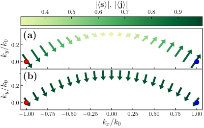
Figure 7: In-plane spin polarization and particle current corresponding to the Fermi-arc surface state for $B=0$, $\alpha/\pi=0.1$, and $\varepsilon=0$, shown as color-scale plots in the $k_{x}$-$k_{y}$ plane, cf. App. B. Red and blue dots indicate the surface projections of the Weyl nodes, arrows show the in-plane components of the spin polarization $\braket{\mathbf{s}}$ [panel (a)] and of the particle current $\braket{\mathbf{j}}$ [panel (b)].

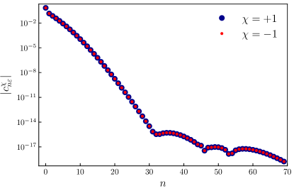
Figure 8: Absolute value of the coefficients $c^{\chi}_{n\varepsilon}$ appearing in the superposition (26) vs order $n$. Note the logarithmic scale for the coefficients. The shown results were obtained by numerically solving Eq. (35) for $\varepsilon/k_{0}=0.1$, $\alpha/\pi=0.1$, $\lambda_{B}=1$, with a cut-off value of $N=70$.

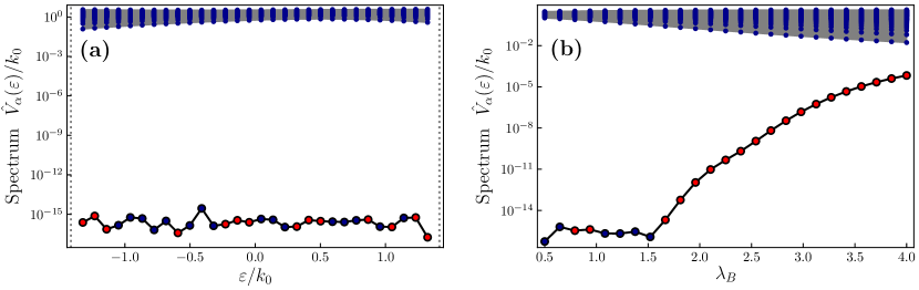
Figure 9: Spectrum of $\hat{V}_{\alpha}$ as obtained from Eq. (28) for $\alpha/\pi=0.1$, with the cut-off value $N=100$. Note the semi-logarithmic scales. Blue (red) dots correspond to positive (negative) eigenvalues. Since $\mathbbm{V}_{\alpha}$ is positive semi-definite, negative eigenvalues indicate numerical errors. (a) Spectrum vs energy $\varepsilon$ (in units of $k_{0}$) in the ultra-quantum regime $|\varepsilon|<\sqrt{2}/\ell_{B}$ delimited by the vertical gray line, for $\lambda_{B}=1$. (b) Spectrum vs $\lambda_{B}$ for $\varepsilon/k_{0}=0.1$.

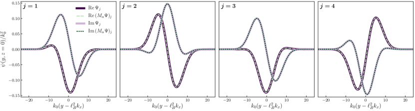
Figure 10: Spinor components $\Psi_{j=1,2,3,4}$ of the eigenstate solution at the surface, $\Psi(y,z=0)=\left(\Psi_{1}(y),\Psi_{2}(y),\Psi_{3}(y),\Psi_{4}(y)\right)^{T}$, compared with the corresponding components of $M_{\alpha}\Psi(y,z=0)$. Parameters are given by $\varepsilon/k_{0}=0.1$, $\alpha/\pi=0.1$ and $\lambda_{B}=3$. We separately show the real and imaginary parts, which verify that the boundary condition $M_{\alpha}\Psi(y,z=0)=\Psi(y,z=0)$ is numerically satisfied to high accuracy.

In this Appendix, we discuss the spin texture related to $s^{\mu}=\sigma^{\mu}\tau^{0}$ (with $\mu=x,y,z$) along a Fermi arc for the $B=0$ case. Getting access to this type of quantity is an advantage of the four-band model with respect to two-band models [50, 51, 47]. Furthermore, we compute the in-plane current $j^{\mu}=\sigma^{\mu}\tau^{z}$ generated by the Fermi arc. Given a normalized Fermi-arc solution $\ket{\Psi}$, we need to evaluate expectation values of the form $\braket{\sigma^{\nu}\tau^{\mu}}=\int^{\infty}_{0}dz\,\Psi^{\dagger}(z)\sigma^{\nu}\tau^{\mu}\Psi(z).$

For a straight arc ($\alpha=0$), the corresponding solutions in Eq. (59) satisfy $\sigma^{y}\ket{\psi^{\chi}}_{\bm{\sigma}}=-\chi\ket{\psi^{\chi}}_{\bm{\sigma}}$, implying $\braket{\mathbf{s}}=k_{x}\hat{\mathbf{e}}_{y}/k_{0}$ and $\braket{\mathbf{j}}=-\hat{\mathbf{e}}_{y}$.

For curved arcs with $\alpha>0$, we use the general solution (61) and perform the integration. The spin polarization follows from

$$\braket{s^{\mu}}=\sum_{\chi=\pm}\frac{|c_{\chi}|^{2}}{2\kappa_{\chi}}\psi^{\chi\,\dagger}(0)\sigma^{\mu}\psi^{\chi}(0),$$ (66)

where the expression for the in-plane current only differs by a relative sign in the sum,

$$\braket{j^{\mu}}=\sum_{\chi=\pm}\chi\frac{|c_{\chi}|^{2}}{2\kappa_{\chi}}\psi^{\chi\,\dagger}(0)\sigma^{\mu}\psi^{\chi}(0).$$ (67)

Above, we have suppressed the momentum dependence of $c_{\chi}$ and of $\ket{\psi^{\chi}}_{\bm{\sigma}}$.

Results obtained from the above expressions are shown in Fig. 7. Our model correctly reproduces the main features of Fermi arcs as experimentally detected. First and foremost, the chiral transport is shown by the current in Fig. 7(b). In addition, the spin polarization rotates along the arc as dictated by the fact that the spin orientation at the two termination points corresponds to the chirality of the Weyl nodes. This behavior is manifest in Fig. 7(a) and in accordance with the spin texture observed experimentally by spin-filtered angle-resolved photoemission spectroscopy [67, 68].

Appendix C Numerical implementation of boundary conditions

In this Appendix, we discuss the numerical approach introduced in Sec. III. Figure 8 shows representative results for the coefficients ${\mathbf{c}}_{\varepsilon}$ in Eq. (26), which are obtained by numerically solving Eq. (35) for a Landau level cut-off $N=70$. These results already indicate that the numerical scheme is well controlled and convergent. A non-trivial benchmark that is passed accurately by our numerical scheme is provided by the analytical solutions (39) and (42) for a DSM with $\alpha=0$ or $\varepsilon=0$, respectively.

Let us next give additional details about our numerical approach. To avoid numerical overflow (or underflow) when computing the matrix elements (27) for a large cut-off $N$, it is convenient to compute the overlaps (33) using the recursion relation ($n\geq m>1$)

$$\braket{\varphi^{-}_{n}}{\varphi^{+}_{m}} =\frac{1}{\sqrt{nm}}\left(n+m-1-2\lambda_{B}^{2}\right)\braket{\varphi^{-}_{n-1}}{\varphi^{+}_{m-1}}$$

$$-\sqrt{\frac{(n-1)(m-1)}{nm}}\braket{\varphi^{-}_{n-2}}{\varphi^{+}_{m-2}},$$ (68)

with

$$\braket{\varphi^{-}_{n-m+1}}{\varphi^{+}_{1}}=\frac{n-m+1-2\lambda_{B}^{2}}{\sqrt{n-m+1}}\braket{\varphi^{-}_{n-m}}{\varphi^{+}_{0}}$$ (69)

and

$$\braket{\varphi^{-}_{n-m}}{\varphi^{+}_{0}}=\sqrt{\frac{2^{n-m}}{(n-m)!}}\lambda_{B}^{n-m}\,\mathrm{e}^{-\lambda_{B}^{2}}.$$ (70)

With these relations, we can easily employ a LL number cut-off of order $N=250$ or even larger. For all results shown in this work, we have carefully checked that results do not change when further increasing the cut-off.

Numerical solutions are then found from the kernel of $V_{\alpha}(\varepsilon)$, i.e., from the matrix representation of $\mathbbm{V}_{\alpha}$ in the subspace with fixed $\varepsilon$ and $k_{x}$. Note that we physically expect a single solution in this subspace in the ultra-quantum regime. Consequently, the spectrum of $V_{\alpha}(\varepsilon)$ should have a single zero eigenvalue which is well separated from all other eigenvalues. Fig. 9 shows representative results for the spectrum of the rescaled matrix $\hat{V}_{\alpha}$ obtained from Eq. (28). We find a non-degenerate, well-separated and vanishing eigenvalue for all $\varepsilon$ in the ultra-quantum regime. However, for $\lambda_{B}\gtrsim 1.5$ (weak magnetic fields), numerical errors become slightly larger. Nonetheless, our numerical solutions still satisfy the boundary condition as demonstrated for $\lambda_{B}=3$ in Fig. 10, where we show the four components of the real and imaginary parts of $\Psi(y,z=0)$ and $M_{\alpha}\Psi(y,z=0)$, respectively. The boundary condition $\Psi(y,z=0)=M_{\alpha}\Psi(y,z=0)$ is indeed satisfied to high precision for all values of $y$.

Appendix D Shift of the reflected electron

The electronic Goos-Hänchen effect is a quantum phenomenon, best described as a lateral shift of a wave packet after reflection from a surface [69]. We can see an analogue of this effect in the system at hand at the level of the expectation value of the position operator. In particular, we can read Eq. (26) in the ultra-quantum regime $0<\varepsilon<\sqrt{2}/\ell_{B}$ as the superposition of an incoming wave in the chiral LL with $\chi=+1$, an outgoing wave in the chiral LL with $\chi=-1$ and a series of bound states, see Eq. (21). Considering first a single momentum component $k_{x}$, the expectation value of the $y$-coordinate for an incoming electron arriving on the surface ($z=0$) is computed from the fundamental eigenmode of the harmonic oscillator in Eq. (19) as $\left\langle y\right\rangle_{\mathrm{in}}=\ell_{B}^{2}\left(k_{x}+k_{0}\right)$. The momentum $k_{x}$ is conserved in the reflection process, and one readily sees that the electron leaving the surface has the expectation value $\left\langle y\right\rangle_{\mathrm{out}}=\ell_{B}^{2}\left(k_{x}-k_{0}\right)$. We note that the shift $\langle y\rangle_{\mathrm{out}}-\langle y\rangle_{\mathrm{in}}$ is gauge invariant.

Following Ref. [69], we now generalize this argument and write an electronic wave packet formed by a superposition of plane waves with various momenta $k_{x}$ and, for simplicity, a Gaussian envelope function centered around momentum $p$ with spread $\Delta k$. Such a wavepacket, in the $\chi=+1$ block, has the form

$$\Psi_{\varepsilon,\rm{in}}(\mathbf{r})=\frac{1}{\sqrt{2\pi}}\int dk_{x}\,F\left(k_{x}-p\right)\mathrm{e}^{ik_{x}x}\psi_{0,\varepsilon}^{+}(y,z),$$ (71)

with $F\left(k_{x}\right)=\left(\sqrt{\pi}\Delta k\right)^{-\frac{1}{2}}\mathrm{e}^{-\frac{1}{2}\left(k_{x}/\Delta k\right)^{2}}$. The expectation value of the $y$-coordinate for the wavepacket arriving on the surface then follows as

$$\left\langle y\right\rangle_{{\rm in}}=\ell_{B}^{2}\left(p+k_{0}\right).$$ (72)

Repeating the calculation for the outgoing wavepacket in the $\chi=-1$ block,

$$\Psi_{\varepsilon,\mathrm{out}}(\mathbf{r})=\frac{1}{\sqrt{2\pi}}\int dk_{x}\,F\left(k_{x}-p\right)e^{ik_{x}x}\psi_{0,\varepsilon}^{-}(y,z),$$ (73)

one finds $\left\langle y\right\rangle_{{\rm out}}=\ell_{B}^{2}\left(p-k_{0}\right)$. We conclude that the electronic Goos-Hänchen shift is given by Eq. (38). As this result is separately valid for each $k_{x}$, we expect it to hold for every choice of the envelope function.

References

- Burkov [2016] A. Burkov, Topological semimetals, Nature Materials 15, 1145 (2016).
- Yan and Felser [2017] B. Yan and C. Felser, Topological materials: Weyl semimetals, Annual Review of Condensed Matter Physics 8, 337 (2017).
- Armitage et al. [2018] N. Armitage, E. Mele, and A. Vishwanath, Weyl and Dirac semimetals in three-dimensional solids, Reviews of Modern Physics 90, 015001 (2018).
- Burkov [2018] A. Burkov, Weyl metals, Annual Review of Condensed Matter Physics 9, 359 (2018).
- Nielsen and Ninomiya [1983] H. B. Nielsen and M. Ninomiya, The Adler-Bell-Jackiw anomaly and Weyl fermions in a crystal, Physics Letters B 130, 389 (1983).
- Hosur and Qi [2013] P. Hosur and X. Qi, Recent developments in transport phenomena in Weyl semimetals, Comptes Rendus Physique 14, 857 (2013).
- Burkov [2015] A. Burkov, Chiral anomaly and transport in Weyl metals, Journal of Physics: Condensed Matter 27, 113201 (2015).
- Gorbar et al. [2018] E. Gorbar, V. Miransky, I. Shovkovy, and P. Sukhachov, Anomalous transport properties of Dirac and Weyl semimetals, Low Temperature Physics 44, 487 (2018).
- Nielsen and Ninomiya [1981] H. B. Nielsen and M. Ninomiya, Absence of neutrinos on a lattice:(I). Proof by homotopy theory, Nuclear Physics B 185, 20 (1981).
- Xu et al. [2015] S.-Y. Xu, I. Belopolski, N. Alidoust, M. Neupane, G. Bian, C. Zhang, R. Sankar, G. Chang, Z. Yuan, C.-C. Lee, et al., Discovery of a Weyl fermion semimetal and topological Fermi arcs, Science 349, 613 (2015).
- Zhang et al. [2016a] C.-L. Zhang, S.-Y. Xu, I. Belopolski, Z. Yuan, Z. Lin, B. Tong, G. Bian, N. Alidoust, C.-C. Lee, S.-M. Huang, et al., Signatures of the Adler–Bell–Jackiw chiral anomaly in a Weyl fermion semimetal, Nature Communications 7, 1 (2016a).
- Hasan et al. [2017] M. Z. Hasan, S.-Y. Xu, I. Belopolski, and S.-M. Huang, Discovery of Weyl fermion semimetals and topological Fermi arc states, Annual Review of Condensed Matter Physics 8, 289 (2017).
- Ong and Liang [2021] N. Ong and S. Liang, Experimental signatures of the chiral anomaly in Dirac–Weyl semimetals, Nature Reviews Physics 3, 394 (2021).
- Potter et al. [2014] A. C. Potter, I. Kimchi, and A. Vishwanath, Quantum oscillations from surface Fermi arcs in Weyl and Dirac semimetals, Nature Communications 5, 5161 (2014).
- Zhang et al. [2016b] Y. Zhang, D. Bulmash, P. Hosur, A. C. Potter, and A. Vishwanath, Quantum oscillations from generic surface Fermi arcs and bulk chiral modes in Weyl semimetals, Scientific Reports 6, 23741 (2016b).
- Zhang et al. [2021] C. Zhang, Y. Zhang, H.-Z. Lu, X. Xie, and F. Xiu, Cycling Fermi arc electrons with Weyl orbits, Nature Reviews Physics 3, 660 (2021).
- Parameswaran et al. [2014] S. Parameswaran, T. Grover, D. Abanin, D. Pesin, and A. Vishwanath, Probing the chiral anomaly with nonlocal transport in three-dimensional topological semimetals, Physical Review X 4, 031035 (2014).
- Baum et al. [2015] Y. Baum, E. Berg, S. Parameswaran, and A. Stern, Current at a distance and resonant transparency in Weyl semimetals, Physical Review X 5, 041046 (2015).
- Hou and Sun [2020] Z. Hou and Q.-F. Sun, Nonlocal correlation mediated by Weyl orbits, Physical Review Research 2, 023236 (2020).
- Gorbar et al. [2014] E. Gorbar, V. Miransky, I. Shovkovy, and P. Sukhachov, Quantum oscillations as a probe of interaction effects in Weyl semimetals in a magnetic field, Physical Review B 90, 115131 (2014).
- Zubkov [2023] M. A. Zubkov, Weyl orbits as probe of chiral separation effect in magnetic Weyl semimetals (2023), arXiv:2311.12712 [cond-mat.mes-hall] .
- Wang et al. [2017] C. Wang, H.-P. Sun, H.-Z. Lu, and X. Xie, 3D quantum Hall effect of Fermi arcs in topological semimetals, Physical Review Letters 119, 136806 (2017).
- Li et al. [2020] H. Li, H. Liu, H. Jiang, and X. Xie, 3D quantum Hall effect and a global picture of edge states in Weyl semimetals, Physical Review Letters 125, 036602 (2020).
- Moll et al. [2016] P. J. Moll, N. L. Nair, T. Helm, A. C. Potter, I. Kimchi, A. Vishwanath, and J. G. Analytis, Transport evidence for Fermi-arc-mediated chirality transfer in the Dirac semimetal Cd3As2, Nature 535, 266 (2016).
- Zhang et al. [2017] C. Zhang, A. Narayan, S. Lu, J. Zhang, H. Zhang, Z. Ni, X. Yuan, Y. Liu, J.-H. Park, E. Zhang, et al., Evolution of Weyl orbit and quantum Hall effect in Dirac semimetal Cd3As2, Nature Communications 8, 1272 (2017).
- Zheng et al. [2017] G. Zheng, M. Wu, H. Zhang, W. Chu, W. Gao, J. Lu, Y. Han, J. Yang, H. Du, W. Ning, et al., Recognition of Fermi-arc states through the magnetoresistance quantum oscillations in Dirac semimetal C d 3 A s 2 nanoplates, Physical Review B 96, 121407 (2017).
- Zhang et al. [2019a] C. Zhang, Y. Zhang, X. Yuan, S. Lu, J. Zhang, A. Narayan, Y. Liu, H. Zhang, Z. Ni, R. Liu, et al., Quantum Hall effect based on Weyl orbits in Cd3As2, Nature 565, 331 (2019a).
- Nishihaya et al. [2019] S. Nishihaya, M. Uchida, Y. Nakazawa, R. Kurihara, K. Akiba, M. Kriener, A. Miyake, Y. Taguchi, M. Tokunaga, and M. Kawasaki, Quantized surface transport in topological Dirac semimetal films, Nature Communications 10, 2564 (2019).
- Nishihaya et al. [2021] S. Nishihaya, M. Uchida, Y. Nakazawa, M. Kriener, Y. Taguchi, and M. Kawasaki, Intrinsic coupling between spatially-separated surface Fermi-arcs in Weyl orbit quantum Hall states, Nature Communications 12, 2572 (2021).
- Chang et al. [2021] M. Chang, H. Geng, L. Sheng, and D. Xing, Three-dimensional quantum Hall effect in Weyl semimetals, Physical Review B 103, 245434 (2021).
- Nguyen et al. [2021] D.-H.-M. Nguyen, K. Kobayashi, J.-E. R. Wichmann, and K. Nomura, Quantum Hall effect induced by chiral Landau levels in topological semimetal films, Physical Review B 104, 045302 (2021).
- Zhang et al. [2019b] C. Zhang, Z. Ni, J. Zhang, X. Yuan, Y. Liu, Y. Zou, Z. Liao, Y. Du, A. Narayan, H. Zhang, et al., Ultrahigh conductivity in Weyl semimetal NbAs nanobelts, Nature Materials 18, 482 (2019b).
- Nair et al. [2020] N. L. Nair, M.-E. Boulanger, F. Laliberté, S. Griffin, S. Channa, A. Legros, W. Tabis, C. Proust, J. Neaton, L. Taillefer, et al., Signatures of possible surface states in TaAs, Physical Review B 102, 075402 (2020).
- Li et al. [2017] P. Li, Y. Wen, X. He, Q. Zhang, C. Xia, Z.-M. Yu, S. A. Yang, Z. Zhu, H. N. Alshareef, and X.-X. Zhang, Evidence for topological type-II Weyl semimetal WTe2, Nature Communications 8, 2150 (2017).
- Bernevig et al. [2022] B. A. Bernevig, C. Felser, and H. Beidenkopf, Progress and prospects in magnetic topological materials, Nature 603, 41 (2022).
- Morali et al. [2019] N. Morali, R. Batabyal, P. K. Nag, E. Liu, Q. Xu, Y. Sun, B. Yan, C. Felser, N. Avraham, and H. Beidenkopf, Fermi-arc diversity on surface terminations of the magnetic Weyl semimetal Co3Sn2S2, Science 365, 1286 (2019).
- Dwivedi [2018] V. Dwivedi, Fermi arc reconstruction at junctions between Weyl semimetals, Physical Review B 97, 064201 (2018).
- Abdulla et al. [2021] F. Abdulla, S. Rao, and G. Murthy, Fermi arc reconstruction at the interface of twisted Weyl semimetals, Physical Review B 103, 235308 (2021).
- Buccheri et al. [2022a] F. Buccheri, R. Egger, and A. De Martino, Transport, refraction, and interface arcs in junctions of Weyl semimetals, Physical Review B 106, 045413 (2022a).
- Kaushik et al. [2022] S. Kaushik, I. Robredo, N. Mathur, L. M. Schoop, S. Jin, M. G. Vergniory, and J. Cano, Transport signatures of Fermi arcs at twin boundaries in Weyl materials (2022), arXiv:2207.14109 [’cond-mat.mes-hall’] .
- Chaou et al. [2023] A. Y. Chaou, V. Dwivedi, and M. Breitkreiz, Magnetic breakdown and chiral magnetic effect at Weyl-semimetal tunnel junctions, Physical Review B 107, L241109 (2023).
- Chaou et al. [2024] A. Y. Chaou, V. Dwivedi, and M. Breitkreiz, Quantum oscillation signatures of interface Fermi arcs, Phys. Rev. B 110, 035116 (2024).
- Breitkreiz and Brouwer [2023] M. Breitkreiz and P. W. Brouwer, Fermi-arc metals, Physical Review Letters 130, 196602 (2023).
- Witten [2016] E. Witten, Three lectures on topological phases of matter, La Rivista del Nuovo Cimento 39, 313 (2016).
- Hashimoto et al. [2017] K. Hashimoto, T. Kimura, and X. Wu, Boundary conditions of Weyl semimetals, Progress of Theoretical and Experimental Physics 2017, 053I01 (2017).
- Thiang [2021] G. C. Thiang, On spectral flow and Fermi arcs, Communications in Mathematical Physics 385, 465 (2021).
- Buccheri et al. [2022b] F. Buccheri, A. De Martino, R. G. Pereira, P. W. Brouwer, and R. Egger, Phonon-limited transport and Fermi arc lifetime in Weyl semimetals, Phys. Rev. B 105, 085410 (2022b).
- Akhmerov and Beenakker [2007] A. Akhmerov and C. Beenakker, Detection of valley polarization in graphene by a superconducting contact, Physical Review Letters 98, 157003 (2007).
- Akhmerov and Beenakker [2008] A. Akhmerov and C. Beenakker, Boundary conditions for Dirac fermions on a terminated honeycomb lattice, Physical Review B 77, 085423 (2008).
- Bovenzi et al. [2018] N. Bovenzi, M. Breitkreiz, T. O’Brien, J. Tworzydło, and C. Beenakker, Twisted Fermi surface of a thin-film Weyl semimetal, New Journal of Physics 20, 023023 (2018).
- Burrello et al. [2019] M. Burrello, E. Guadagnini, L. Lepori, and M. Mintchev, Field theory approach to the quantum transport in Weyl semimetals, Physical Review B 100, 155131 (2019).
- Gradshteyn and Ryzhik [2014] I. S. Gradshteyn and I. M. Ryzhik, Table of integrals, series, and products (Academic press, 2014).
- Saykin et al. [2018] D. R. Saykin, K. S. Tikhonov, and Y. I. Rodionov, Landau levels with magnetic tunneling in a Weyl semimetal and magnetoconductance of a ballistic p-n junction, Physical Review B 97, 041202 (2018).
- Chan and Lee [2017] C.-K. Chan and P. A. Lee, Emergence of gapped bulk and metallic side walls in the zeroth Landau level in Dirac and Weyl semimetals, Physical Review B 96, 195143 (2017).
- Sundaram and Niu [1999] G. Sundaram and Q. Niu, Wave-packet dynamics in slowly perturbed crystals: Gradient corrections and Berry-phase effects, Physical Review B 59, 14915 (1999).
- Wawrzik et al. [2021] D. Wawrzik, J.-S. You, J. I. Facio, J. Van Den Brink, and I. Sodemann, Infinite Berry Curvature of Weyl Fermi Arcs, Physical Review Letters 127, 056601 (2021).
- Wigner [1955] E. P. Wigner, Lower Limit for the Energy Derivative of the Scattering Phase Shift, Phys. Rev. 98, 145 (1955).
- Smith [1960] F. T. Smith, Lifetime Matrix in Collision Theory, Phys. Rev. 118, 349 (1960).
- Abdulla et al. [2022] F. Abdulla, A. Das, S. Rao, and G. Murthy, Time-reversal-broken Weyl semimetal in the Hofstadter regime, SciPost Physics Core 5, 014 (2022).
- Benito-Matías et al. [2020] E. Benito-Matías, R. A. Molina, and J. González, Surface and bulk Landau levels in thin films of Weyl semimetals, Physical Review B 101, 085420 (2020).
- Yao et al. [2017] H. Yao, M. Zhu, L. Jiang, and Y. Zheng, Simulation on the electronic wave packet cyclotron motion in a Weyl semimetal slab, Journal of Physics: Condensed Matter 29, 155502 (2017).
- Abdulla [2024] F. Abdulla, Pairwise annihilation of Weyl nodes induced by magnetic fields in the Hofstadter regime, Physical Review B 109, 155142 (2024).
- Tchoumakov et al. [2017] S. Tchoumakov, M. Civelli, and M. O. Goerbig, Magnetic description of the Fermi arc in type-I and type-II Weyl semimetals, Physical Review B 95, 125306 (2017).
- Behrends et al. [2019] J. Behrends, S. Roy, M. H. Kolodrubetz, J. H. Bardarson, and A. G. Grushin, Landau levels, Bardeen polynomials, and Fermi arcs in Weyl semimetals: Lattice-based approach to the chiral anomaly, Physical Review B 99, 140201 (2019).
- Belopolski et al. [2019] I. Belopolski, K. Manna, D. S. Sanchez, G. Chang, B. Ernst, J. Yin, S. S. Zhang, T. Cochran, N. Shumiya, H. Zheng, et al., Discovery of topological Weyl fermion lines and drumhead surface states in a room temperature magnet, Science 365, 1278 (2019).
- Liu et al. [2019] D. Liu, A. Liang, E. Liu, Q. Xu, Y. Li, C. Chen, D. Pei, W. Shi, S. Mo, P. Dudin, et al., Magnetic Weyl semimetal phase in a Kagomé crystal, Science 365, 1282 (2019).
- Lv et al. [2015] B. Q. Lv, S. Muff, T. Qian, Z. D. Song, S. M. Nie, N. Xu, P. Richard, C. E. Matt, N. C. Plumb, L. X. Zhao, G. F. Chen, Z. Fang, X. Dai, J. H. Dil, J. Mesot, M. Shi, H. M. Weng, and H. Ding, Observation of Fermi-Arc Spin Texture in TaAs, Phys. Rev. Lett. 115, 217601 (2015).
- Xu et al. [2016] S.-Y. Xu, I. Belopolski, D. S. Sanchez, M. Neupane, G. Chang, K. Yaji, Z. Yuan, C. Zhang, K. Kuroda, G. Bian, C. Guo, H. Lu, T.-R. Chang, N. Alidoust, H. Zheng, C.-C. Lee, S.-M. Huang, C.-H. Hsu, H.-T. Jeng, A. Bansil, T. Neupert, F. Komori, T. Kondo, S. Shin, H. Lin, S. Jia, and M. Z. Hasan, Spin Polarization and Texture of the Fermi Arcs in the Weyl Fermion Semimetal TaAs, Phys. Rev. Lett. 116, 096801 (2016).
- Chen et al. [2013] X. Chen, X.-J. Lu, Y. Ban, and C.-F. Li, Electronic analogy of the Goos-Hänchen effect: a review, Journal of Optics 15, 033001 (2013).