An Adaptive Second-order Method for a Class of Nonconvex Nonsmooth Composite Optimization

Abstract

This paper explores a specific type of nonconvex sparsity-promoting regularization problems, namely those involving $\ell_{p}$-norm regularization, in conjunction with a twice continuously differentiable loss function. We propose a novel second-order algorithm designed to effectively address this class of challenging nonconvex and nonsmooth problems, showcasing several innovative features: (i) The use of an alternating strategy to solve a reweighted $\ell_{1}$ regularized subproblem and the subspace approximate Newton step. (ii) The reweighted $\ell_{1}$ regularized subproblem relies on a convex approximation to the nonconvex regularization term, enabling a closed-form solution characterized by the soft-thresholding operator. This feature allows our method to be applied to various nonconvex regularization problems. (iii) Our algorithm ensures that the iterates maintain their sign values and that nonzero components are kept away from 0 for a sufficient number of iterations, eventually transitioning to a perturbed Newton method. (iv) We provide theoretical guarantees of global convergence, local superlinear convergence in the presence of the Kurdyka-Łojasiewicz (KL) property, and local quadratic convergence when employing the exact Newton step in our algorithm. We also showcase the effectiveness of our approach through experiments on a diverse set of model prediction problems.

1 Introduction

Consider the nonconvex regularized sparse optimization problem in the following form,

$$\underset{\bm{x}\in\mathbb{R}^{n}}{\min} F(\bm{x}):=f(\bm{x})+\lambda\sum_{i=1}^{n}r(|x_{i}|),$$ (1)

where $f:\mathbb{R}^{n}\to\mathbb{R}$ is a twice continuously differentiable function, $r:\mathbb{R}\to\mathbb{R}$ is smooth on $\mathbb{R}\backslash\{0\}$, concave and strictly increasing on $\mathbb{R}_{+}$ with $r_{i}(0)=0$. $\lambda>0$ is the regularization parameter.

Various regularizations fitting this problem have been introduced, such as Minimax Concave Penalty [1], Smoothly Clipped Absolute Deviation [2] and Cappled $\ell_{1}$ [3]. These regularizations serve as approximations to the $\ell_{0}$-norm regularization and consistently provide less biased estimates for nonzero components compared to the LASSO problem. Given the efficiency of numerous first-order [4, 5, 6] and second-order methods [7, 8, 9] in solving the LASSO problem, much work has focused on solving these types of problems.

The $\ell_{p}$-norm $(0<p<1)$ regularization is a well-known representative of these problems, attracting significant attention in recent years due to its strong properties. Particularly for $p=1/2$, this method demonstrates a markedly enhanced sparsity-promoting ability compared to $\ell_{1}$ regularization [10]. In this paper, we first consider the $\ell_{p}$-norm regularization optimization problem as follows

$$\underset{\bm{x}\in\mathbb{R}^{n}}{\text{minimize}} F(\bm{x}):=f(\bm{x})+\lambda\|\bm{x}\|_{p}^{p}. \mathscr{P}$$ ()

Problem Equation $\mathscr{P}$ has been proven to be strongly NP-hard [11] due to the nonconvex and nonsmooth nature of the $\ell_{p}$ norm term. In practical applications, $\ell_{p}$ regularization can be used to foster sparser solutions while preserving some beneficial aspects of convex regularization. This approach has found extensive application across various fields, including compressed sensing, signal processing, machine learning and statistics [12, 13, 14, 15].

A variety of approximating methods have been developed to address Problem $\mathscr{P}$, as detailed in studies by Lu [16], Wang et al. [17, 18, 19], Lai [20], Chen [21] and others [22, 23, 24, 25]. These methods tackle the nonconvexity and nonsmoothness of $\ell_{p}$-term using different approximation $\phi$. For example,

$$\phi_{1}(x_{i})=\max\{\mu,|x_{i}|^{p}\},\quad\phi_{2}(x_{i})=p(|x^{k}_{i}|^{\alpha}+\epsilon_{i})^{\frac{p}{\alpha}-1}|x_{i}|^{\alpha}.$$

with $\mu>0,\alpha\geq 1,\bm{\epsilon}\geq 0$, $\bm{x}^{k}$ being the current iterate. $\phi_{1}$ was introduced by Lu et al. [16], who constructed a Lipschitz continuous approximation around zero. $\phi_{2}$ is recognized as the iteratively reweighted $\ell_{1}$($\ell_{2}$) method when $\alpha=1$($\alpha=2$). This approach constructs a convex approximation by employing weights derived from the linearization of the $\ell_{p}$ norm at the current iterate, a strategy that has been extensively considered in many first order methods [20, 17, 18, 19]. Wang et al. [17] proposed an iterative reweighted $\ell_{1}$ method using iterative soft-thresholding update, the basic iterative step reads as follows:

$$\bm{x}^{k+1}\in\operatornamewithlimits{argmin}_{\bm{x}\in\mathbb{R}^{n}}\left\{\langle\nabla f(\bm{x}),\bm{x}\rangle+\frac{\alpha}{2}\|\bm{x}-\bm{x}^{k}\|^{2}+\sum^{n}_{i=1}p(|x^{k}_{i}|+\epsilon_{i})^{p-1}|x_{i}|\right\},$$

where $\alpha>0$ is a constant relating to the Lipschitz constant of $f$. Moreover, significant advancements have been made by Yu [26] and Wang et al. [19] by incorporating the extrapolation technique into the iteratively reweighted $\ell_{1}$ methods. These authors established convergence results concerning perturbations under the Kurdyka- Łojasiewicz (KL) property. Chen [21] introduced a second-order method utilizing a smoothing trust region Newton approach for Problem 1, which approximates the regularizer with a twice continuously differentiable function. This method tackles the nonsmoothness of the $|\cdot|$ operator using an iterative reweighted $\ell_{2}$ approximation and demonstrates global convergence to a local minimizer. In these methods, the perturbation $\bm{\epsilon}$ plays a crucial role in the design of algorithms and in achieving convergence results. Wang et al. [17] developed a dynamic updating strategy that drives the perturbation associated with nonzero components towards zero while maintaining the others as constants. For $p=\tfrac{1}{2}$ and $\tfrac{2}{3}$, the proximal gradient method is extensively used. Xu [24] provides a closed-form proximal mapping for these specific values of $p$. Although exact and inexact numerical methods for generic $\ell_{p}$ proximal mapping have been proposed [27, 28], these methods are considerably slower than the closed-form solution and may sometimes be considered unaffordable for large-scale problems. Several first-order methods that capitalize on these developments have been introduced in recent works [10, 29].

Second-order methods have focused extensively on general nonconvex and nonsmooth composite problems. Inspired by proximal mapping, a class of proximal Newton methods has emerged [30, 31, 32, 33]. These methods require regularizer to be convex and solve the following regularized proximal Newton problem globally, achieving a superlinear convergence rate under various assumptions (metric $q(>1/2)$-subregularity assumption for [32], Luo-Tseng error Bound for [31], KL property for [33]).

$$\bm{x}^{k+1}\in\operatornamewithlimits{argmin}_{\bm{x}\in\mathbb{R}^{n}}\left\{\langle\nabla f(\bm{x}),\bm{x}\rangle,+\frac{1}{2}\langle\bm{x}-\bm{x}^{k},H^{k}(\bm{x}-\bm{x}^{k})\rangle+g(\bm{x})\right\},$$

where $H^{k}$ is the hessian approximation at iterate $\bm{x}^{k}$, $g(\cdot)$ is the regularization function.

Considering the specific sparsity-driven Problem 1, it exhibits a nature where the nonsmooth regularization functions usually present a smooth substructure, involving active manifolds where the functions are locally smooth. For instance, in Problem $\mathscr{P}$, the function is smooth around any point strictly bounded away from zero. Although $\bm{x}=0$ is a natural stationary point of $F$ (see 6 for the optimal condition), it is not a desirable solution in terms of objective value. Therefore, identifying an appropriate active manifold becomes a critical step in addressing these problems. The proximal gradient method and its variants have proven effective in reaching the optimal submanifold [34, 35]. The manifold identification complexity of different variants of the proximal gradient method is detailed in [36]. The iteratively reweighted method shares similar properties with the proximal gradient method, as their iterative forms and optimal conditions align (see 11). From this perspective, we have designed an automatic active manifold identification process using the iteratively reweighted method. After identifying a relatively optimal active manifold, transitioning to a Newton method is a logical step, as it is widely recognized that first-order methods are fast for global convergence but slow for local convergence. Employing a Newton method on the smooth active manifold typically yields a superlinear convergence rate. A class of hybrid methods for nonconvex and nonsmooth composite problems has been explored, utilizing a forward-backward envelope approach that integrates proximal gradient with Newton method [37, 38, 39]. However, few second-order methods specifically tailored for Problem $\mathscr{P}$ have been proposed until recently. Wu et al. [40] introduced a hybrid approach combining the proximal gradient method with the subspace regularized Newton method, demonstrated to achieve a superlinear convergence rate under the framework of the Kurdyka-Łojasiewicz theory.

In this paper, we design and analyze second-order methods for the $\ell_{p}$-norm regularization problem (Problem $\mathscr{P}$), which are also applicable to general nonconvex and nonsmooth regularization problems (Problem 1). Our method is a hybrid approach that alternates between solving an iteratively reweighted $\ell_{1}$ subproblem and a subspace Newton subproblem. This hybrid framework integrates the subspace Newton method with a subspace iterative soft-thresholding technique, employing an approximate solution for the Newton subproblem to enhance algorithmic speed. Unlike proximal-type methods, each iteration of our method approximates the $\ell_{p}$-norm with a weighted $\ell_{1}$-norm and locally accelerates the process using the Newton direction.

The adaptability of the Newton subproblem allows our method to incorporate various types of quadratic programming (QP) subproblems, achieving diverse convergence outcomes based on the subsolver employed. The proposed method achieves global convergence under the conditions of Lipschitz continuity of the function $f$ and boundedness of the Hessian (see 3). Locally, we establish the convergence rate under the Kurdyka-Łojasiewicz (KL) property of $F$ with different exponents, achieving superlinear convergence with an exponent of 1/2. By employing a strategic perturbation setting, we attain local quadratic convergence under the local Hessian Lipschitz continuity of $F$ on the support. When extending our method to tackle the generic problems (Problem 1), the same convergence results are maintained.

Numerical experiments for Problem $\mathscr{P}$ demonstrate the superior performance of our approach compared to existing methods, such as a hybrid method combining the proximal gradient and regularized Newton methods [40], and an extrapolated iteratively reweighted $\ell_{1}$ method [19]. Our method shows notable advantages in time efficiency while maintaining comparable solution quality against existing first-order and second-order methods. Additional experiments on various regularization fitting problems (Problem 1) validate our algorithm’s effectiveness across different settings.

Our work presents several distinguishing features compared to existing second-order methods. Unlike the smoothing trust region Newton method [21], which requires a twice continuously differentiable approximation for regularization terms, our method uses a nonsmooth local model that retains the form of weighted $\ell_{1}$ regularization and optimizes within a subspace, potentially yielding more efficient and targeted search directions. Moreover, our method dynamically identifies and exploits the active manifold during the optimization process, a feature not present in the smoothing trust region Newton method. Furthermore, unlike the hybrid method of proximal gradient and regularized Newton methods (HpgSRN) [40], which uses a proximal gradient method across the entire space to identify the active manifold, our method applies iterative soft thresholding updates on the subspaces of zero and nonzero components separately, enhancing and clarifying the identification process. This distinct approach allows our method to adopt an iteratively reweighted $\ell_{1}$ structure globally and shift to the original problem locally.

1.1 Organization

The rest of this paper is organized as follows. §2 includes notation and the characterization of optimal condition for the problem. §3 presents the algorithm and explain the design logic. §4 provides the global and local convergence analysis of our algorithm. §5.2 provides another local subproblem for our algorithm and extends our algorithm to generic nonconvex and nonsmooth sparsity-driven regularization problems. §6 shows the numerical experiments on the logistic regression problem and demonstrate its performance through both synthetic and real datasets against PG Newton method HpgSRN[40] and iteratively reweighted first-order method EPIR$\ell_{1}$[19].

2 Preliminaries

2.1 Notation

Let $\mathbb{R}_{++}^{n}=\{\bm{x}\in\mathbb{R}^{n}\mid x_{i}>0\}$. For any $\bm{x}\in\mathbb{R}^{n}$, we use $x_{i}$ to denote its $i$th component. For any symmetric matrix $M\in\mathbb{R}^{n\times n}$, define $M_{{\cal I}}$ as the submatrix of $M$ with rows and columns indexed by ${\cal I}$. Denote $\mathbb{R}^{{\cal I}}$ the subspace consisting of the variables in ${\cal I}$ and setting the rest as zero, i.e.,

$$\mathbb{R}^{{\cal I}}:=\{\bm{x}\in\mathbb{R}^{n}\mid x_{i}=0,i\in{\cal I}^{c}\}.$$

For a nonempty set ${\cal S}$, let $|{\cal S}|$ denote its cardinality. Define $[n]=\{1,2,3,\ldots,n\}$. Let $\text{sign}(x_{i})=1$ if $x_{i}>0$, $\text{sign}(x_{i})=-1$ if $x_{i}<0$ and $\text{sign}(x_{i})=0$ if $x_{i}=0$. Define the set of nonzeros and zeros of $\bm{x}$ as

$${\cal I}(\bm{x})=\{i\mid x_{i}\neq 0\}\quad\text{ and }\quad{\cal I}_{0}(\bm{x})=\{i\mid x_{i}=0\},$$

respectively. ${\cal I}(\bm{x})$ is also known as the support of $\bm{x}$, and is further partitioned into ${\cal I}(\bm{x})={\cal I}_{+}(\bm{x})\cup{\cal I}_{-}(\bm{x})$ where

$${\cal I}_{+}(\bm{x})=\{i\mid x_{i}>0\}\ \text{ and }\ {\cal I}_{-}(\bm{x})=\{i\mid x_{i}<0\}.$$

Given $\bm{v}\in\mathbb{R}^{n}$ and $\bm{\omega}\in\mathbb{R}^{n}_{++}$, the weighted soft-thresholding operator is defined as

$$[\mathbb{S}_{\bm{\omega}}(\bm{v})]_{i}:=\text{sign}(v_{i})\max(|v_{i}|-\omega_{i},0).$$

For $\bm{x},\bm{y}\in\mathbb{R}^{n}$, let $\bm{x}\circ\bm{y}$ denote the component-wise product: $[\bm{x}\circ\bm{y}]_{i}=x_{i}y_{i},i\in[n]$.

In $\mathbb{R}^{n}$, let $\|\bm{x}\|$ denote the Euclidean norm of $\bm{x}$ and the $\|\bm{x}\|_{p}:=(\sum_{i=1}^{n}|x_{i}|^{p})^{\frac{1}{p}}$ denotes the $\ell_{p}$ norm of $\bm{x}$ (it is a norm if $p\geq 1$ and a quasi-norm if $0<p<1$). If function $f:\mathbb{R}^{n}\rightarrow\mathbb{R}\cup\{+\infty\}$ is convex, then the subdifferential of $f$ at $\bar{\bm{x}}$ is given by

$$\partial f(\bar{\bm{x}}):=\{\bm{z}|f(\bar{\bm{x}})+\langle\bm{z},\bm{x}-\bar{\bm{x}}\rangle\leq f(\bm{x}),\forall\bm{x}\in\mathbb{R}^{n}\}.$$

If function $f$ is lower semi-continuous, then the Frechet subdifferential of $f$ at $\bm{a}$ is given by

$$\partial_{F}f(\bm{a}):=\{\bm{z}\in\mathbb{R}^{n}|\liminf_{\bm{x}\to\bm{a}}\frac{f(\bm{x})-f(\bm{a})-\langle\bm{z},\bm{x}-\bm{a}\rangle}{\|\bm{x}-\bm{a}\|_{2}}\geq 0\}$$

and the limiting subdifferential of $f$ at $\bm{a}$ is given by

$$\bar{\partial}f(a):=\{\bm{z}^{*}=\lim_{\bm{x}^{k}\to\bm{a},f(\bm{x}^{k})\to f(\bm{a})}z^{k},z^{k}\in\partial_{F}f(\bm{x}^{k})\}.$$

We abuse our notation by writing $\nabla_{i}F(\bm{x})=\nabla_{x_{i}}F(\bm{x})=\frac{\partial}{\partial x_{i}}F(\bm{x})$ if $F$ is (partially) differentiable with respect to $x_{i}$; we do not suggest $\nabla_{i}F(\bm{x})=[\nabla F(\bm{x})]_{i}$ since $F$ may not be differentiable at $\bm{x}$. In addition, if $F$ is differentiable with respect to a set of variables $x_{i},i\in{\cal I}$, $\nabla_{\cal I}F(\bm{x})$ and $\nabla_{x_{\cal I}}F(\bm{x})$ is the gradient subvector of $\nabla_{i}F(\bm{x}),i\in{\cal I}$. Also denote $\nabla_{{\cal I}{\cal I}}F(\bm{x})$ as the subspace Hessian of $F$ with respect to ${\cal I}$ if $F$ is (partially) smooth of $x_{i},{\cal I}$.

2.2 Optimality conditions for Reweighted algorithm

The first-order necessary optimality condition for Problem $\mathscr{P}$ is given by [16]

$$x_{i}\nabla_{i}f(\bm{x})+\lambda p|x_{i}|^{p}=0\text{ for all }i=1,\ldots,n.$$ (2)

Any point satisfying condition (2) is called a first-order optimal solution. In particular, the zero vector always satisfies (2). The first-order optimality condition (2) is equivalent to

$$\nabla_{i}f(\bm{x})+\lambda p|x_{i}|^{p-1}\text{sign}(x_{i})=0\text{ for all }i\in{\cal I}(\bm{x}).$$ (3)

Thus, solving for a first-order optimal solution essentially involves identifying the support set. Once the nonzero elements of the optimal solution are accurately identified, the problem simplifies to a smooth problem.

In our algorithm, we first add relaxation parameter $\bm{\epsilon}\in\mathbb{R}_{++}^{n}$ to form an approximated objective function, that is

$$\underset{\bm{x}\in\mathbb{R}^{n}}{\text{minimize}} F(\bm{x};\bm{\epsilon}):=f(\bm{x})+\lambda\sum_{i=1}^{n}(|x_{i}|+\epsilon_{i})^{p},$$ (4)

where $\epsilon_{i}>0$ for all $i=1,\ldots,n$. The first-order optimal condition of (4) is

$$0\in\nabla_{i}f(\bm{x})+\omega_{i}\partial|x_{i}|\quad\text{ for all }i=1,\ldots,n,$$ (5)

where $\omega_{i}:=\bm{\omega}(x_{i},\epsilon_{i})=\lambda p(|x_{i}|+\epsilon_{i})^{p-1}$ for all $i=1,\ldots,n$. An equivalent form of (5) is written as

$$|\nabla_{i}f(\bm{x})|\leq\omega_{i},\quad i\in{\cal I}_{0}(\bm{x}),$$ (6)

$$\nabla_{i}f(\bm{x})+\omega_{i}\text{sign}(x_{i})=0,\quad i\in{\cal I}(\bm{x}).$$

Also, notice that

$$\text{ \eqref{eq.relaxedopcondition} is satisfied and }\epsilon_{i}=0,i\in{\cal I}(\bm{x})\iff\text{ \eqref{eq.optimalcondition} is satisfied}.$$ (7)

3 Algorithm

We describe the details of the proposed method in this section.

3.1 Local approximation

Our algorithm is based on constructing a weighted $\ell_{1}$ local model of $F$ at the $k$th iteration, which is formulated as

$$G^{k}(\bm{x}):=f(\bm{x})+\sum_{i=1}^{n}\omega^{k}_{i}|x_{i}|,$$ (8)

where $\omega^{k}_{i}=\lambda p(|x^{k}_{i}|+\epsilon^{k}_{i})^{p-1}$ and $\omega^{k}_{i}=\infty$ if $x^{k}_{i}=0$ and $\epsilon^{k}_{i}=0$. The optimal condition at each iteration is

$$0\in\nabla_{i}f(\bm{x})+\bm{\omega}^{k}_{i}\partial|x_{i}|\quad\text{ for all }i=1,\ldots,n.$$ (9)

The following lemma provides a connection between the (weighted) $\ell_{1}$-regularized model $G^{k}(\bm{x})$ and $F(\bm{x};\bm{\epsilon}^{k})$.

Lemma 1.

It holds for any $\bm{\epsilon}^{k+1}\leq\bm{\epsilon}^{k}$ that

$$F(\bm{x}^{k+1},\bm{\epsilon}^{k+1})-F(\bm{x}^{k},\bm{\epsilon}^{k})\leq F(\bm{x}^{k+1},\bm{\epsilon}^{k})-F(\bm{x}^{k},\bm{\epsilon}^{k})\leq G^{k}(\bm{x}^{k+1})-G^{k}(\bm{x}^{k}).$$ (10)

Moreover, the following are equivalent:

• $\bm{x}^{k}$ is first-order optimal for $G^{k}(\bm{x})$.

• $\bm{x}^{k}$ is first-order optimal for $F(\bm{x};\bm{\epsilon}^{k})$.

• $\bm{x}^{k}=\mathbb{S}_{\bm{\omega}^{k}}(\bm{x}^{k}-\nabla f(\bm{x}^{k}))$.

Proof.

We first prove (10). According to the expression of $F$ and $G$, it suffices to show that

$$(|x_{i}^{k+1}|+\epsilon_{i}^{k})^{p}-(|x_{i}^{k}|+\epsilon_{i}^{k})^{p}\leq\omega^{k}_{i}(|x_{i}^{k+1}|-|x^{k}_{i}|).$$

This is true since $(|x_{i}^{k+1}|+\epsilon_{i}^{k})^{p}-(|x_{i}^{k}|+\epsilon_{i}^{k})^{p}\leq\omega^{k}_{i}(|x_{i}^{k+1}|-|x^{k}_{i}|)$ by the concavity of $|\cdot|^{p}$ and $\epsilon_{i}^{k+1}\leq\epsilon^{k}_{i}$.

The rest of the statement is true by noticing that

$$\bm{x}^{k}\text{ is optimal for }G^{k}(\bm{x})\iff \ (\bm{x}^{k}+\partial\langle\bm{\omega}^{k},|\cdot|\rangle)\ni(\bm{x}^{k}-\nabla f(\bm{x}^{k}))$$ (11)

$$\iff \ \bm{x}^{k}=\mathbb{S}_{\bm{\omega}^{k}}(\bm{x}^{k}-\nabla f(\bm{x}^{k}))$$

$$\iff \ \eqref{eq.relaxedopcondition}\text{ is satisfied}$$

$$\iff \ \bm{x}^{k}\text{ is optimal for }F(\bm{x};\bm{\epsilon}^{k}),$$

completing the proof. ∎

Our approach solves different subproblems based on the progress made by the current zero components and nonzeros for minimizing $F(\bm{x};\bm{\epsilon})$. For this purpose, we define the complementary optimality residual pairs $\Psi(\bm{x};\bm{\epsilon})$ and $\Phi(\bm{x};\bm{\epsilon})$ caused by zeros and nonzeros at $(\bm{x};\bm{\epsilon})$, respectively,

$$[\Psi(\bm{x};\bm{\epsilon})]_{i}:=\begin{cases}\nabla_{i}f(\bm{x})+\omega_{i},&\text{if }i\in{\cal I}_{0}(\bm{x})\text{ and }\nabla_{i}f(\bm{x})+\omega_{i}<0,\\ \nabla_{i}f(\bm{x})-\omega_{i},&\text{if }i\in{\cal I}_{0}(\bm{x})\text{ and }\nabla_{i}f(\bm{x})-\omega_{i}>0,\\ 0,&\text{otherwise;}\end{cases}$$ (12)

$$[\Phi(\bm{x};\bm{\epsilon})]_{i}:=\text{\hskip 219.08612pt}\\$$ (13)

$$\begin{cases}0,&\text{if }i\in{\cal I}_{0}(\bm{x}),\\ \min\{\nabla_{i}f(\bm{x})+\omega_{i},\max\{x_{i},\nabla_{i}f(\bm{x})-\omega_{i}\}\},&\text{if }i\in{\cal I}_{+}(\bm{x})\text{ and }\nabla_{i}f(\bm{x})+\omega_{i}>0,\\ \max\{\nabla_{i}f(\bm{x})-\omega_{i},\min\{x_{i},\nabla_{i}f(\bm{x})+\omega_{i}\}\},&\text{if }i\in{\cal I}_{-}(\bm{x})\text{ and }\nabla_{i}f(\bm{x})-\omega_{i}<0,\\ \nabla_{i}f(\bm{x})+\omega_{i}\cdot\text{sign}(x_{i}),&\text{otherwise.}\end{cases}$$

If $(\bm{x};\bm{\epsilon})$ satisfies condition (5), then $|\nabla_{i}f(\bm{x})|\leq\omega_{i}$ holds true for any $i\in{\cal I}_{0}(\bm{x})$. This suggests that the size of $\Psi(\bm{x};\bm{\epsilon})_{i}$ reflects how far are the zero components from being optimal for $F(\bm{x};\bm{\epsilon})$ at $(\bm{x};\bm{\epsilon})$. On the other hand, for $i\in{\cal I}_{+}(\bm{x})\cup{\cal I}_{-}(\bm{x})$, the optimality conditions (5) imply that $\nabla f(\bm{x})+\bm{\omega}\cdot\text{sign}(x_{i})=0$. Therefore, the size of $\Phi(\bm{x};\bm{\epsilon})$ implies how far are the nonzeros from being optimal for $F(\bm{x};\bm{\epsilon})$ at $(\bm{x};\bm{\epsilon})$. The definition also takes into account how far nonzero components might shift before they turn to zero within $\Phi$.

The following lemma summarizes the understanding of these measures.

Proposition 1.

(i) For any $(\bm{x};\bm{\epsilon})$ with $\bm{\epsilon}\in\mathbb{R}^{n}_{++}$ and $\bm{\omega}=\bm{\omega}(\bm{x};\bm{\epsilon})$, it holds that

$$|[\Phi(\bm{\bm{x}};\bm{\epsilon})]_{i}|\leq\left|\nabla_{i}F(\bm{x};\bm{\epsilon})\right|,\ i\in{\cal I}(\bm{x}).$$ (14)

(ii) Letting $d(\mu):=\mathbb{S}_{\mu\bm{\omega}}(\bm{x}-\mu\nabla f(\bm{x}))-\bm{x}$ for $\mu>0$, the following decomposition holds

$$\Psi(\bm{x};\bm{\epsilon})+\Phi(\bm{x};\bm{\epsilon})=-d(1).$$ (15)

More generally,

$$d_{i}(\mu) =-\mu[\Psi(\bm{x};\bm{\epsilon})]_{i} \text{ if }\ i\in{\cal I}_{0}(\bm{x}),$$ (16)

$$|d_{i}(\mu)| \geq\min\{\mu,1\}|[\Phi(\bm{x};\bm{\epsilon})]_{i}| \text{ if }\ i\in{\cal I}(\bm{x}).$$ (17)

(iii) Therefore, $\bm{x}$ satisfies the first-order optimal condition (6) if

$$\|\Phi(\bm{x};\bm{\epsilon})\|=\|\Psi(\bm{x};\bm{\epsilon})\|=0.$$ (18)

Additionally, if $\epsilon_{i}=0$ for $i\in{\cal I}(\bm{x})$ in $\bm{\omega}$, then (18) implies that $\bm{x}$ satisfies the first-order optimal condition (3).

Proof.

(i) If $i\in{\cal I}_{+}(\bm{x})$, $\nabla_{i}F(\bm{x};\bm{\epsilon})=\nabla_{i}f(\bm{x})+\omega_{i}$. In the last case in the definition of $\Phi(\bm{x};\bm{\epsilon})$, $[\Phi(\bm{x};\bm{\epsilon})]_{i}=\nabla_{i}f(\bm{x})+\omega_{i}=\nabla_{i}F(\bm{x};\bm{\epsilon})$. In the second case, $[\Phi(\bm{x};\bm{\epsilon})]_{i}=\min\{\nabla_{i}f(\bm{x})+\omega_{i},x_{i}\}\leq\nabla_{i}f(\bm{x})+\omega_{i}$ if $\nabla_{i}f(\bm{x})-\omega_{i}<0$, and otherwise $[\Phi(\bm{x};\bm{\epsilon})]_{i}=\min\{\nabla_{i}f(\bm{x})+\omega_{i},\nabla_{i}f(\bm{x})-\omega_{i}\}\leq\nabla_{i}f(\bm{x})+\omega_{i}$. Overall, (14) holds.

If $i\in{\cal I}_{-}(\bm{x})$, we have (14) still holds true by the same argument.

(ii) (15) is true by [7, Lemma A.1], meaning $\Psi(\bm{x};\bm{\epsilon})=-d_{i}(1)$, $i\in{\cal I}_{0}(\bm{x})$ and $\Phi(\bm{x};\bm{\epsilon})=-d_{i}(1)$, $i\in{\cal I}(\bm{x})$ by the complementarity of $\Psi$ and $\Phi$. This, together with Lemma 6, implies that (16) and (17).

Therefore, if (18) is satisfied, (15) and (11) imply that (6) is satisfied. In addition, if $\epsilon_{i}=0,i\in{\cal I}(\bm{x})$, it follows from (7) that $\bm{x}$ satisfies the first-order optimal condition (3).

(iii) Obvious. ∎

The reason why we use different optimality residuals for zero and nonzero components is that our approach is a subspace method of minimizing different sets of variables at each iteration. These two residuals are used in our approach as the “switching sign” of optimizing the zero components or the nonzeros. Specifically, if $\|\Psi^{k}\|\geq\gamma\|\Phi^{k}\|$ for prescribed $\gamma\in(0,1)$, it indicates that at $\bm{x}^{k}$ the zero components have relatively greater impact on the optimality error than the nonzero components. The algorithm solves a subproblem that only involves the variables that are zero in the current iterate. Conversely, if $\|\Psi^{k}\|\geq\gamma\|\Phi^{k}\|$, indicating that at $\bm{x}^{k}$ the nonzero components have a relatively greater impact on the optimality error than the zero components, only the variables that are nonzero in current iterate appear in the subproblem.

3.2 Updating of $\bm{\epsilon}$ and termination

Proposition 1 implies that the algorithm converges to an optimal solution of $F(\bm{x})$ if $\max\{\|\Psi^{k}\|,\|\Phi^{k}\|\}\to 0$ and $\epsilon^{k}_{i}\to 0,i\in{\cal I}^{k}$. This gives our termination criterion (line 2–line 4) It also implies that the updating strategy for $\bm{\epsilon}$ should drive $\epsilon^{k}_{i}$ rapidly to zero once the correct support ${\cal I}^{k}$ is detected. On the other hand, we would want $\epsilon^{k}_{i},i\in{\cal I}_{0}^{k}$ be fixed as constants once the correct support is detected. The central reason this strategy is to eliminate the zeros and the associated $\epsilon_{i}$ from $F(\bm{x};\bm{\epsilon})$ so that the problem resembles a smooth problem, which plays a crucial role in the convergence analysis.

For this purpose, our updating strategy only reduces $\epsilon_{i}$ associated with the nonzeros in $\bm{x}^{k}$, i.e., $\epsilon^{k}_{i}\in(0,\beta\epsilon^{k}_{i})$, $i\in{\cal I}^{k}$ where $\beta\in(0,1)$ is prescribed (line 6) This dynamically updating strategy was first proposed in [17] and was proved to be able to stop the updating of $\epsilon_{i}$ associated with the zeros in the optimal solution while consecutively decreasing $\epsilon_{i}$ associated with the nonzeros in the optimal solution for sufficiently large $k$.

3.3 Support detection step

The purpose of our algorithm is to dynamically detect the support of the optimal solution using a first-order subproblem during the iteration; as the support eventually is found, the algorithm reverts to a second-order (Newton) subproblem involving the nonzero variables to trigger fast local convergence.

At the core of the support detection phase is to solving a weighted $\ell_{1}$ norm regularized subproblem of a subset ${\cal W}$ of the variables

$$\underset{x_{\cal W}\in\mathbb{R}^{|{\cal W}|}}{\min}\left\{\langle\nabla_{\cal W}f(\bm{x}^{k}),x_{\cal W}\rangle+\tfrac{1}{2\mu}\|x_{\cal W}-\bm{x}^{k}_{\cal W}\|_{2}^{2}+\sum_{i\in{\cal W}}\bm{\omega}^{k}_{i}|x_{i}|\right\}$$ (19)

with closed-form solution $[\mathbb{S}_{\mu\bm{\omega}^{k}}(\bm{x}^{k}-\mu\nabla f(\bm{x}^{k}))]_{\cal W}$. For sufficiently small $\mu$, subproblem (19) renders a descent direction for $G^{k}$ and therefore is also descent for $F$, as is shown in the convergence analysis. Therefore, whenever solving a subproblem (19), a backtracking strategy is used to find a proper value of $\mu$ such that sufficient decrease $G^{k}(\bm{x}^{j})<G^{k}(\bm{x})-\frac{\alpha}{2}\|\bm{x}^{j}-\bm{x}\|^{2}$ is achieved for a prescribed $\alpha$. The solution of this subproblem is stated in subroutine Algorithm 2, and is referred to as the iterative soft-thresholding (IST) step.

Lemma 2.

The backtracking linesearch procedure in Algorithm 2 (line 2–8) terminates finitely with iteration $\ell$, satisfying $\min\{\bar{\mu},\frac{\xi}{L_{1}(\bm{x})+\alpha}\}\leq\mu^{\ell}\leq\bar{\mu}$ with $L_{1}(\bm{x})>0$ being the local Lipschitz constant of $f$ in a neigborhood of $\bm{x}$ and

$$F(\bm{x}^{\ell};\bm{\epsilon})-F(\bm{x};\bm{\epsilon})\leq-\frac{\alpha}{2}\|\bm{x}^{\ell}-\bm{x}\|^{2}.$$

Proof.

Assume Algorithm 2 is triggered at the $k$th iteration by calling $\hat{\bm{x}}=\text{IST}(\bm{x},\bm{\omega},{\cal W};\alpha,\xi,\bar{\mu})$. For simplicity, we remove the superscript $k$ for outer loop in the subroutine Algorithm 2. For any $j$, $x_{{{\cal W}^{c}}}^{j}=x_{{{\cal W}^{c}}}$ and $x_{\cal W}^{j}=[\mathbb{S}_{\mu^{j}\bm{\omega}}(\bm{x}-\mu^{j}\nabla f(\bm{x}))]_{\cal W}$. Since $x_{\cal W}(\mu)=[\mathbb{S}_{\mu\bm{\omega}}(\bm{x}-\mu\nabla f(\bm{x}))]_{\cal W}$ is continuous with respect to $\mu\in(0,\bar{\mu}]$. Therefore, we can consider a neigborhood of $\bm{x}$ containing $x_{\cal W}(\mu),\forall\mu\in(0,\bar{\mu}]$, on which $f$ is Lipschitz differentiable with constant $L_{1}(\bm{x})$. By the optimality of $\bm{x}^{j}$ for subproblem (19),

$$\langle\nabla f(\bm{x}),\bm{x}^{j}-\bm{x}\rangle+\frac{1}{2\mu^{j}}\|\bm{x}^{j}-\bm{x}\|^{2}+\sum_{i=1}^{n}\omega_{i}|\bm{x}^{j}_{i}|\leq\sum_{i=1}^{n}\omega_{i}|x_{i}|.$$ (20)

It follows that for any $\mu^{j}\leq\tfrac{1}{L_{1}(\bm{x})+\alpha}$,

$$G(\bm{x}^{j}) \leq f(\bm{x})+\langle\nabla f(\bm{x}),\bm{x}^{j}-\bm{x}\rangle+\frac{L_{1}(\bm{x})}{2}\|\bm{x}^{j}-\bm{x}\|^{2}+\sum_{i=1}^{n}\omega_{i}|\bm{x}^{j}_{i}|$$

$$\leq f(\bm{x})+\langle\nabla f(\bm{x}),\bm{x}^{j}-\bm{x}\rangle+\frac{1}{2\mu^{j}}\|\bm{x}^{j}-\bm{x}\|^{2}+\sum_{i=1}^{n}\omega_{i}|\bm{x}^{j}_{i}|-\frac{\alpha}{2}\|\bm{x}^{j}-\bm{x}\|^{2}$$

$$\leq f(\bm{x})+\sum_{i=1}^{n}\omega_{i}|x_{i}|-\frac{\alpha}{2}\|\bm{x}^{j}-\bm{x}\|^{2}$$

$$=G(\bm{x})-\frac{\alpha}{2}\|\bm{x}^{j}-\bm{x}\|^{2}$$

Therefore, the backtracking procedure terminates with $\mu^{\ell}\geq\min\{\bar{\mu},\frac{\xi}{L_{1}(\bm{x})+\alpha}\}$. ∎

An important property of subproblem (19) is the local support stable property of the iterates, meaning the iterates generated by this subproblem have unchanged sign value and the nonzeros are uniformly bounded away from 0 for sufficiently large $k$. This property was first found by [17] and played a crucial role in the complexity analysis [18] and extrapolation analysis [19]. Therefore, this supbroblem in the initial phase of the algorithm and the second-order (Newton) subproblem is then triggered only if it renders unchanged support.

3.4 Subspace second-order subproblem

If it is shown that two consecutive iterates have an unchanged sign, we formulate the second-order subproblem consisting of the nonzero variables (line 16–18)

$$\min_{d\in\mathbb{R}^{|{\cal W}^{k}|}}m^{k}(d):=\langle g^{k},d\rangle+\frac{1}{2}\langle d,H^{k}d\rangle,$$ (21)

where $H^{k}$ and $g^{k}$ are chosen as subspace Hessian matrix and gradient of problem $F(\bm{x}^{k};\bm{\epsilon}^{k})$ and working index set ${\cal W}^{k}\subset{\cal I}(\bm{x}^{k})$. In this way, the $F(\bm{x};\bm{\epsilon})$ is smooth with respect to the variables in ${\cal W}^{k}$ around $\bm{x}^{k}$. Since $m^{k}$ is constructed in the reduced space $\mathbb{R}^{|{\cal W}^{k}|}$, it may have small dimension. Therefore, it can be easily handled by existing efficient quadratic programming solvers, e.g., Conjugate Gradient (CG) method. We do not have any requirement for the selection of subproblem solver.

If the correct support is eventually detected and an exact subspace Hessian of $F$ is employed in a neighborhood of the optimal solution, the algorithm then reverts to a classic Newton method for solving nonlinear problems. Otherwise, we have to take care of the unboundedness of the subproblem. One popular technique is to modify the Hessian by a multiple of identity matrix to ensure positive definiteness (line 16), which yields a descent direction. The other technique is to include a trust region to avoid the unboundedness, which often needs a tailored solver to find the (global) optimal solution of the subproblem. We shall discuss the possible variants in later section.

It should be noticed that we do not require an exact minimizer of $m^{k}$ is found by the subproblem solver in each iteration. Let $d_{R}^{k}$ be a reference direction which is computed (line 17) by minimizing $m^{k}$ along the steepest descent direction. We allow an inexact minimizer of $m^{k}$ as long as the solution $\bar{d}^{k}$ causes a reduction in $m^{k}$ and more descent than $d^{k}_{R}$ (line 18), which is equivalent to requiring $m^{k}(\bar{d}^{k})\leq m^{k}(0)$ and $\langle g^{k},\bar{d}^{k}\rangle\leq\langle g^{k},d_{R}^{k}\rangle$. We only use $\bar{d}^{k}$ to update the variables in ${\cal W}^{k}$, so that the search direction $d^{k}\in\mathbb{R}^{n}$ is set accordingly (line 19). Therefore, after (inexact) solution of the QP subproblem, we end up with the following result.

Lemma 3.

If the QP subproblem (21) is solved (line 16–19 of Algorithm 1) with positive definite $H^{k}$, then the following hold

$$\langle g^{k},\bar{d}^{k}\rangle\leq \ \langle g^{k},d_{R}^{k}\rangle<0,$$ (22)

$$|\langle g^{k},\bar{d}^{k}\rangle|\geq \ |\langle g^{k},d_{R}^{k}\rangle|=\frac{\|g^{k}\|^{2}}{\langle g^{k},H^{k}g^{k}\rangle}\|g^{k}\|^{2}\geq\frac{\|g^{k}\|^{2}}{\lambda_{\max}(H^{k})},$$ (23)

$$\frac{\|g^{k}\|}{\lambda_{\max}(H^{k})} \leq\|\bar{d}^{k}\|\leq\frac{2\|g^{k}\|}{\lambda_{\min}(H^{k})}.$$ (24)

Proof.

We only have to prove (24). Let $d^{k}_{N}$ be the exact solution of the QP subproblem (21) satisfying $H^{k}d^{k}_{N}=-g^{k}$, meaning $d^{k}_{N}$ is the minimizer of $m^{k}(d)$. It follows that

$$\|d^{k}_{N}\|\leq\|(H^{k})^{-1}\|\|g^{k}\|\leq\frac{\|g^{k}\|}{\lambda_{\min}(H^{k})}.$$ (25)

Let us also define the quadratic function $\bar{m}^{k}(d):=m^{k}(d_{N}^{k}+d)$ and the associated level set $\mathcal{L}^{k}:=\{d:\bar{m}^{k}(d)\leq 0\}$. We then see that

$$(\bar{d}^{k}-d_{N}^{k})\in\mathcal{L}^{k},$$ (26)

since $\bar{m}^{k}(\bar{d}^{k}-d^{k}_{N})=m^{k}(\bar{d}^{k})\leq m^{k}(0)=0$ (required by line 18 of Algorithm 1). For $d\in{\cal L}^{k}$, we have

$$\lambda_{\min}(H^{k})\|d\|^{2}<\langle d,H^{k}d\rangle\leq-\langle g^{k},d_{N}^{k}\rangle,$$

where the second inequality can be directly inferred from the definition of ${\cal L}^{k}$. Therefore, for $d$ is up bounded by

$$\|d\|^{2}<\frac{-\langle g^{k},d_{N}^{k}\rangle}{\lambda_{\min}(H^{k})}.$$

Combining this with (25), the definition of $d_{N}^{k}$, and (26) shows that

$$\|\bar{d}^{k}-d^{k}_{N}\|^{2}\leq\frac{-\langle g^{k},d_{N}^{k}\rangle}{\lambda_{\min}(H^{k})}\leq\frac{\|(H^{k})^{-1}\|\|g^{k}\|^{2}}{\lambda_{\min}(H^{k})}=\frac{\|g^{k}\|^{2}}{(\lambda_{\min}(H^{k}))^{2}}.$$

By combining this inequality with the triangle inequality and (25), we obtain

$$\|\bar{d}^{k}\|\leq\|\bar{d}^{k}-d^{k}_{N}\|+\|d^{k}_{N}\|\leq\frac{\|g^{k}\|}{\lambda_{\min}(H^{k})}+\frac{\|g^{k}\|}{\lambda_{\min}(H^{k})}=\frac{2\|g^{k}\|}{\lambda_{\min}(H^{k})}.$$

In addition, $\|\bar{d}^{k}\|\geq\frac{\|g^{k}\|}{\lambda_{\max}(H^{k})}$ is straightforward from (23). ∎

3.5 Projected line search

Once a descent direction for $F$ is obtained by solving the QP subproblem, the algorithm calls the subrountine Algorithm 3 of the projected line search to determine a stepsize ensuring a sufficient decrease in $F(\bm{x};\bm{\epsilon})$. This strategy was first proposed by [7]. The line search use the function $\text{Proj}(\cdot;\bm{x}^{k})$ to project a given vector onto the subspace containing $\bm{x}^{k}$,

$$[\text{Proj}(\bm{y};\bm{x}^{k})]_{i}:=\begin{cases}\max\{0,y_{i}\}&\text{if }{\cal I}_{+}(\bm{x}^{k}),\\ \min\{0,y_{i}\}&\text{if }{\cal I}_{-}(\bm{x}^{k}),\\ 0&\text{if }{\cal I}_{0}(\bm{x}^{k}).\end{cases}$$

First of all, a backtracking procedure searches along the direction $d^{k}$ to determine a step size $\mu^{j}$ such that the projection of $\text{Proj}(\bm{x}^{k}+\mu^{j}d^{k})$ causes a decrease in $G^{k}$ (line 1–8). If such a stepsize is found, it is deemed as a successful step and the line search subroutine is terminated with $\bm{x}^{k+1}\leftarrow\text{Proj}(\bm{x}^{k}+\mu^{j}d^{k})$. Otherwise, $\text{Proj}(\bm{x}^{k}+\mu^{j}d^{k})$ must encounter the same sign of $\bm{x}^{k}$ after finite trials; in this case, the backtracking procedure fails and is terminated with $j>0$.

The failure of the backtracking procedure indicates that it is hopeless to find a successful new iterate with smaller support than $\bm{x}^{k}$. As a result, the algorithm verifies the largest step size $\mu_{B}$ yielding a new iterate with the same support as $\bm{x}^{k}$ (line 9–15). If $\bm{x}^{k}+\mu_{B}d^{k}$ causes a sufficient decrease in $G^{k}$, then it is again deemed as a successful step and the line search subroutine is terminated.

The definition of $\mu_{B}$ implies that $\mu_{B}$ is no less than the $\mu^{j}$ found in the backtracking procedure. Therefore, if $\mu_{B}$ is successful, then the final loop will not be triggered. On the contrary, if $\mu_{B}$ is unsuccessful, the final loop (line 16–22) continue with the backtracking procedure which is generally known to terminate in finite trials. Since now the trail point $\bm{y}^{j}$ must have the same sign as $\bm{x}^{k}$, there is no need to call $\text{Proj}(\cdot;\bm{x}^{k})$. For the whole procedure, we conclude ${\cal I}(\bm{x}^{k+1})={\cal I}(\bm{x}^{k})$ if the subroutine Algorithm 3 terminates in line 18 and ${\cal I}(\bm{x}^{k+1})\subset{\cal I}(\bm{x}^{k})$ otherwise.

Lemma 4.

Given $d$ and ${\cal W}\subset{\cal I}(\bm{x})$ satisfying $\langle\nabla_{{\cal W}}F(\bm{x};\bm{\epsilon}),d_{{\cal W}}\rangle<0$ and $d_{{\cal W}^{c}}=0$, then Algorithm 3 terminates finitely with iteration $\ell$. Furthermore, if $\text{sign}(\bm{y}^{\ell})\neq\text{sign}(\bm{x})$, $\mu^{\ell}$ satisfying

$$\mu^{\ell}\geq\min(1,\mu_{B}),\quad|{\cal I}(\bm{y}^{\ell})|<|{\cal I}(\bm{x})|$$ (27)

if $\text{sign}(\bm{y}^{\ell})=\text{sign}(\bm{x})$,

$$\mu^{\ell}\geq\frac{2\xi(\eta-1)\langle\nabla_{{\cal W}}F(\bm{x};\bm{\epsilon}),d_{{\cal W}}\rangle}{L_{2}(\bm{x})\|d_{{\cal W}}\|^{2}},$$ (28)

where $L_{2}(\bm{x})$ is the Lipschitz constant of $F(\bm{x};\bm{\epsilon})$ in the neigborhood ${\cal B}(\bm{x},\xi\alpha_{B}\|d\|)$ of $\bm{x}$ in the subspace $\mathbb{R}^{{\cal W}}$.

Proof.

Since $x_{\cal W},{\cal W}\subset{\cal I}(\bm{x})$ is in the interior of the “subspace orthant” $\{z_{\cal W}\mid\text{sign}(z_{\cal W})=\text{sign}(x_{\cal W})\}$ and $F(\bm{x};\bm{\epsilon})$ is smooth in the subspace orthant around $x_{\cal W}$, we can remove the subscript ${\cal W}$ for brevity.

If $\text{sign}(\bm{y}^{\ell})\neq\text{sign}(\bm{x})$, then Algorithm 3 terminates by line 4 or line 13. Therefore, $F(\bm{y}^{\ell};\bm{\epsilon})\leq F(\bm{x};\bm{\epsilon})$ naturally holds and $\bm{y}^{\ell}$ is on the boundary of subspace orthant containing $\bm{x}$, meaning $|{\cal I}(\bm{y}^{\ell})|<|{\cal I}(\bm{x})|$.

If $\text{sign}(\bm{y}^{\ell})=\text{sign}(\bm{x})$, then Algorithm 3 executes line 16–22 and terminates by line 18. When line 16 is reached, there are two cases to consider.

If $j=0$, then $\bm{x}+d$ and $\bm{x}$ are contained in the same orthant. In this case, there is no points of nondifferentiability of $F(\bm{x};\bm{\epsilon})$ exist on the line segment connecting $\bm{x}$ to $\bm{x}+d$. This also means $\mu^{0}=1$ when reaching line 16. The backtracking line search terminates with .

If $j>0$, then line 10 in 14 are executed but the condition in line 12 is violated. Notice that $\bm{x}+\mu_{B}d$ is on the boundary of the orthant containing $\bm{x}$ and there is also no points of nondifferentiability of $F(\bm{x};\bm{\epsilon})$ exist on the line segment connecting $\bm{x}$ to $\bm{x}+\mu_{B}d$. This also means $\mu^{j}\geq\xi\mu_{B}$ when reaching line 16.

In both cases, we end up with a traditional backtracking line search with $F(\bm{x};\bm{\epsilon})$ $L_{2}(\bm{x})$-Lipschitz differentiable in a neigborhood of $\bm{x}$ (e.g., a ball centered at $\bm{x}$ with radius $\xi\alpha_{B}\|d\|$: ${\cal B}(\bm{x},\xi\alpha_{B}\|d\|)$). Now applying Taylor’s Theorem,

$$F(\bm{x}+\mu d;\bm{\epsilon}) \leq F(\bm{x};\bm{\epsilon})+\mu\langle\nabla F(\bm{x};\bm{\epsilon}),d\rangle+\frac{1}{2}\mu^{2}L_{2}(\bm{x})\|d\|^{2}$$

$$\leq F(\bm{x};\bm{\epsilon})+\eta\mu\langle\nabla F^{k}(\bm{x}),d^{k}\rangle,$$

where the second inequality is satisfies for any

$$\mu\in\bigg{(}0,\frac{2(\eta-1)\langle\nabla F(\bm{x};\bm{\epsilon}),d\rangle}{L_{2}(\bm{x})\|d\|^{2}}\bigg{]}.$$

Therefore, the backtracking line search terminates with $\mu$ satisfying (28). ∎

Algorithm 1 Second-Order Iteratively Reweighted $\ell_{1}$ method (SOIR$\ell_{1}$)

0:  $\{\bm{x}^{0};\bm{\epsilon}^{0}\}\in\mathbb{R}^{n}$; $\{\eta_{\Phi},\eta_{\Psi}\}\in(0,1]$, $\{\beta,\xi\}\in(0,1)$, $\{\bar{\mu},\gamma,\tau,\alpha\}\in(0,\infty)$ and $\eta\in(0,1/2]$.

1:  for $k=0,1,2,\ldots$ do

2:     while $\max\{\|\Psi^{k}\|,\|\Phi^{k}\|\}\leq\tau$  do

3:        if $\epsilon^{k}_{i}\leq\tau,i\in{\cal I}^{k}$ then

4:           return  the (approximate) solution $\bm{x}^{k}$ of Problem Equation $\mathscr{P}$.

5:        else

6:           Set $\epsilon^{k}_{i}\in(0,\beta\epsilon^{k}_{i})$, $i\in{\cal I}^{k}$.

7:        end if

8:     end while

9:     if $\|\Psi^{k}\|\geq\gamma\|\Phi^{k}\|$ then

10:        Choose ${\cal W}^{k}\subseteq\{i:\Psi^{k}_{i}\neq 0\}$ such that $\|[\Psi^{k}]_{{\cal W}^{k}}\|\geq\eta_{\Psi}\|\Psi^{k}\|.$

11:        Call Algorithm 2 to compute $(\bm{x}^{k+1},\mu^{k})\leftarrow\text{IST}(\bm{x}^{k},\bm{\omega}^{k},{\cal W}^{k};\alpha,\xi,\bar{\mu})$.

12:     else

13:        Choose ${\cal W}^{k}\subseteq\{i:\Phi^{k}_{i}\neq 0\}$ such that $\|[\Phi^{k}]_{{\cal W}^{k}}\|\geq\eta_{\Phi}\|\Phi^{k}\|.$

14:        Call Algorithm 2 to compute $(\hat{\bm{x}}^{k+1},\mu^{k})\leftarrow\text{IST}(\bm{x}^{k},\bm{\omega}^{k},{\cal W}^{k};\alpha,\xi,\bar{\mu})$.

15:        if  $\text{sign}(\hat{\bm{x}}^{k+1})=\text{sign}(\bm{x}^{k})$ then

16:           Set $H^{k}\leftarrow\nabla^{2}_{{\cal W}^{k}}F(\bm{x}^{k};\bm{\epsilon}^{k})+\zeta I\succ 0$ and $g^{k}\leftarrow\nabla_{{\cal W}^{k}}F(\bm{x}^{k};\bm{\epsilon}^{k})$.

17:           Compute reference direction $d^{k}_{R}\leftarrow-\frac{\|g^{k}\|^{2}}{\langle g^{k},H^{k}g^{k}\rangle}g^{k}$.

18:           Compute any

$$\bar{d}^{k}\approx\operatornamewithlimits{argmin}\langle g^{k},d\rangle+\frac{1}{2}\langle d^{k},H^{k}d^{k}\rangle,$$

such that the following inequalities hold:

$$\langle g^{k},\bar{d}\rangle\leq\langle g^{k},d^{k}_{R}\rangle\text{ and }m^{k}(\bar{d}^{k})\leq m^{k}(0).$$

19:           Set $d^{k}_{{\cal W}^{k}}=\bar{d}^{k}$, $d^{k}_{{{\cal W}^{k}}^{c}}=0$.

20:           Use Algorithm 3 to compute $(\bm{x}^{k+1},\mu^{k})\leftarrow\text{PLS}(\bm{x}^{k};\bm{\epsilon}^{k},d^{k},{\cal W}^{k};\eta,\xi)$.

21:        else

22:           Set $\bm{x}^{k+1}\leftarrow\hat{\bm{x}}^{k+1}$.

23:        end if

24:     end if

25:     Update $\epsilon_{i}^{k+1}\in(0,\beta\epsilon^{k}_{i})$, $i\in{\cal I}^{k+1}$.

26:     Update $\omega_{i}^{k+1}=\lambda p(|x^{k+1}_{i}|+\epsilon_{i}^{k+1})^{p-1}$, $i\{\in 1,\ldots,n\}$.

27:  end for

Algorithm 2 IST subproblem: $[\bm{x}^{j},\mu^{j}]:=\text{IST}(\bm{x},\bm{\omega},{\cal W};\alpha,\xi,\bar{\mu})$

0:  $\{\bm{x},\bm{\omega}\}\in\mathbb{R}^{n}$, ${\cal W}\in[n]$; $\{\bar{\mu},\alpha\}\in(0,+\infty),\xi\in(0,1)$.

1:  Let $\mu^{0}\leftarrow\bar{\mu}$ and $\bm{x}_{{{\cal W}^{c}}}^{0}\leftarrow\bm{x}_{{{\cal W}^{c}}}$, $\bm{x}^{0}_{{\cal W}}\leftarrow[\mathbb{S}_{\mu^{0}\bm{\omega}}(\bm{x}-\mu^{0}\nabla f(\bm{x}))]_{{\cal W}}$.

2:  for $j=0,1,2,\ldots$ do

3:     if $G^{k}(\bm{x}^{j})<G^{k}(\bm{x})-\frac{\alpha}{2}\|\bm{x}^{j}-\bm{x}\|^{2}$ then

4:        return  $\bm{x}^{j}$.

5:     end if

6:     $\mu^{j+1}\leftarrow\xi\mu^{j}$.

7:     $\bm{x}_{{{\cal W}^{c}}}^{j+1}\leftarrow\bm{x}_{{{\cal W}^{c}}}$, $\bm{x}^{j+1}_{{\cal W}}\leftarrow[\mathbb{S}_{\mu^{j+1}\bm{\omega}}(\bm{x}-\mu^{j+1}\nabla f(\bm{x}))]_{{\cal W}}$.

8:  end for

Algorithm 3 Projected line search: $[\bm{y}^{j},\mu^{j}]:=\text{PLS}(\bm{x};\bm{\epsilon},d,{\cal W};\eta,\xi)$

0:  $\{\bm{x},d;\bm{\epsilon}\}\in\mathbb{R}^{n}$, ${\cal W}\subseteq[n]$; $\eta\in(0,\frac{1}{2})$, $\xi\in(0,1)$.

1:  Set $j\leftarrow 0$, $\mu^{0}\leftarrow 1$ and $\bm{y}^{0}\leftarrow\text{Proj}(\bm{x}+d;\bm{x}).$

2:  while $\text{sign}(\bm{y}^{j})\neq\text{sign}(\bm{x})$ do

3:     if $F(\bm{y}^{j};\bm{\epsilon})\leq F(\bm{x};\bm{\epsilon})$ then

4:        return  $\bm{y}^{j}$.

5:     end if

6:     Set $j\leftarrow j+1$ and $\mu^{j}=\xi\mu^{j-1}$.

7:     Set $\bm{y}^{j}\leftarrow\text{Proj}(\bm{x}+\mu^{j}d;\bm{x})$.

8:  end while

9:  if $j\neq 0$ then

10:     Set $\mu_{B}\leftarrow\text{argsup}\{\mu>0:\text{sign}(\bm{x}+\mu d)=\text{sign}(\bm{x})\}.$

11:     Set $\bm{y}^{j}\leftarrow\bm{x}+\mu_{B}d$.

12:     if $F(\bm{y}^{j};\bm{\epsilon})\leq F(\bm{x};\bm{\epsilon})+\eta\mu_{B}\langle\nabla_{{\cal W}}F(\bm{x};\bm{\epsilon}),d_{{\cal W}}\rangle$ then

13:        return  $\bm{y}^{j}$.

14:     end if

15:  end if

16:  loop

17:     if $F(\bm{y}^{j};\bm{\epsilon})\leq F(\bm{x};\bm{\epsilon})+\eta\mu^{j}\langle\nabla_{{\cal W}}F(\bm{x};\bm{\epsilon}),d_{{\cal W}}\rangle$ then

18:        return  $\bm{y}^{j}$.

19:     end if

20:     Set $j\leftarrow j+1$ and $\mu^{j}=\xi\mu^{j-1}$.

21:     Set $\bm{y}^{j}\leftarrow\bm{x}+\mu^{j}d$.

22:  end loop

3.6 Algorithm description

We are now ready to state our entire proposed second-order iteratively reweighted $\ell_{1}$ algorithm, hereinafter named SOIR$\ell_{1}$, in Algorithm 1, and explain it as follows. Let $\Psi^{k}=\Psi^{k}$ and $\Phi^{k}=\Phi^{k}$. If the termination criterion is not satisfied, there are two cases to consider.

Case (i): $\|\Psi^{k}\|\geq\gamma\|\Phi^{k}\|$. A subset of current zero components

$${\cal W}^{k}\subseteq\{i:\Psi^{k}_{i}\neq 0\}\subseteq{\cal I}_{0}^{k}$$ (29)

is chosen (line 10) such that the norm of $\Psi^{k}$ over ${\cal W}^{k}$ is greater than a certain percentage of $\Psi^{k}$ over all components. We perform in line 11 a subspace IST step as described in Section 3.3 . Since only zero components is chosen in ${\cal W}^{k}$, we conclude ${\cal I}^{k}\subset{\cal I}^{k+1}$, meaning zero components could become nonzero in this step. In fact, by (16), Lemma 2 and (29), $x^{k+1}_{i}=x^{k+1}_{i}-x^{k}_{i}=\mu^{k}\Psi^{k}\neq 0,i\in{\cal W}^{k}$,

$${\cal I}^{k+1}={\cal I}^{k}\cup{\cal W}^{k},\quad|{\cal I}^{k+1}|=|{\cal I}^{k}|+|{\cal W}^{k}|.$$ (30)

Case (ii): $\|\Psi^{k}\|<\gamma\|\Phi^{k}\|$. A subset of nonzeros

$${\cal W}^{k}\subseteq\{i:\Phi^{k}_{i}\neq 0\}\subseteq{\cal I}^{k}$$

is chosen (line 13) such that the norm of $\Phi^{k}$ over this subset is greater than a certain percentage of $\Phi^{k}$ over all components. A IST subproblem is then performed (line 14) to detect whether the sign value of the solution is unchanged (line 15). If this is not the case, then the solution is accepted as the next iterate (line 22) Since only nonzero components is chosen in ${\cal W}^{k}$, we conclude ${\cal I}(\bm{x}^{k})\supset{\cal I}(\bm{x}^{k+1})$, meaning zero components could become nonzero in this step.

If the sign value of the IST subproblem solution remains the same as current iterate, the QP subproblem Equation 21 is then solved (line 16–20) to obtain the search direction $d^{k}$. Since this case is deemed as in a local neigborhood of a optimal solution contained in the interior of the orthant. Therefore, we use the projected line search subrountine Algorithm 3 to determine a stepsize, as described in Section 3.5.

To summarize, we have proved our proposed algorithm is well-posed in that each subproblem is well-defined and will terminate finitely. Moreover, we can make the following conclusion from the above discussion and Lemma 2, Lemma 3 and Lemma 4.

Theorem 2 (Well-posedness).

If $\tau=0$, the overall Algorithm 1 will produce an infinite sequence of iterates $\{(\bm{x}^{k},\bm{\epsilon}^{k})\}$ satisfying $\{F(\bm{x}^{k},\bm{\epsilon}^{k})\}$ and $\{\bm{\epsilon}^{k}\}$ are both monotonically decreasing.

4 Convergence Analysis

The convergence properties of the proposed algorithm are the subject of this section. We make the following assumption for the objective function.

Assumption 3.

• the level set $\mathcal{L}:=\{\bm{x}:F(\bm{x})\leq F(\bm{x}^{0},\bm{\epsilon}^{0})\}$ is contained in a bounded ball $\{\bm{x}\mid\|\bm{x}\|\leq R\}$ so that $f$ Lipschitz differentiable on ${\cal L}$ with constant $L>0$.

• For $H^{k}$ obtained from line 16 in Algorithm 1, there exist $0<\lambda_{\min}<\lambda_{\max}<+\infty$ such that, $\lambda_{\min}I\preceq H^{k}\preceq\lambda_{\max}I$.

In addition, we set the tolerance $\tau=0$.

Theorem 2 implies that the iterates $\{\bm{x}^{k}\}\subset{\cal L}$, so that the local Lipschitz constant of $f$ in Lemma 2 satisfies $L_{1}(\bm{x})\leq L$ and can be replaced with $L$. Moreover, $\lambda_{\min}(H^{k})$ and $\lambda_{\max}(H^{k})$ in Lemma 3 can be replaced with $\lambda_{\min}$ and $\lambda_{\max}$, respectively. As for the Lipschitz constant $L_{2}(\bm{x})$ of $F(\bm{x};\bm{\epsilon})$ restricted in the subspace in Lemma 4, it is also uniformly bounded above if the nonzeros in all the iterates are uniformly bounded from 0. This property is analyzed in the next subsection.

4.1 Support detection

We prove the iterates have stable sign value for sufficiently large $k$, meaning ${\cal I}^{k}$ and ${\cal I}^{k}_{0}$ remain unchanged for sufficiently large $k$.

Theorem 4.

Suppose $\{\bm{x}^{k}\}$ is generated by Algorithm 1. The following hold true.

1. There exists $\delta>0$ such that $|x^{k}_{i}|>\delta,i\in{\cal I}^{k}$ holds true for all $k$. Therefore, $\omega^{k}_{i}<\hat{\omega}:=\lambda p\delta^{p-1},i\in{\cal I}^{k}$ holds true for all $k$.

2. There exist ${\cal I}_{0}^{*},{\cal I}^{*}$ such that ${\cal I}_{0}^{k}\equiv{\cal I}_{0}^{*},{\cal I}^{k}\equiv{\cal I}^{*}$ for sufficiently large $k$.

3. For any limit point $\bm{x}^{*}$ of $\{\bm{x}^{k}\}$, ${\cal I}_{0}(\bm{x}^{*})={\cal I}_{0}^{*}$ and ${\cal I}(\bm{x}^{*})={\cal I}^{*}$.

Proof.

(i) Suppose by contradiction that this is not true. Then there exists a subsequence ${\cal S}\in\mathbb{N}$ and $j\in[n]$ such that

$$|{\cal S}|=\infty,\ \{|x_{j}^{k}|\}\subset\mathbb{R}_{++}\ \text{ and }\ \{|x_{j}^{k}|\}_{{\cal S}}\to 0,$$ (31)

meaning $\lim\limits_{\begin{subarray}{c}k\to\infty\\ k\in{\cal S}\end{subarray}}\omega_{j}^{k}=\infty$ and $\lim\limits_{k\to\infty}\bm{\epsilon}^{k}_{j}=0$.

We first show that there for all sufficiently large $k\in{\cal S}$ such that $x_{j}^{k+1}=0$. Notice that if index $j$ must be chosen by line 13 in Algorithm 1 for an infinite number of times. Otherwise, $x_{j}^{k}$ will remain unchanged for sufficiently large $k$—a contradiction. Suppose $j$ is selected by line 13 at sufficiently large $k\in{\cal S}$ with

$$\mu^{k+1}\omega_{j}^{k}\geq\min\{\bar{\mu},\tfrac{\xi}{L+\alpha}\}\omega_{j}^{k}>R+\max\{\bar{\mu},1\}L>|x_{j}^{k}-\mu^{k+1}\nabla_{j}f(\bm{x}^{k})|;$$ (32)

this can be done since $\{\nabla_{j}f(\bm{x}^{k})\}$ and $\{x_{j}^{k}\}$ are all bounded by 3(i) and $\min\{\bar{\mu},\frac{\xi}{L+\alpha}\}\leq\mu^{k}\leq\bar{\mu}$ by Lemma 2 and 3(i). Lemma 6 implies that $d_{i}(\mu^{k+1})=-x_{j}^{k}$. In other words, line 14 returns $\hat{\bm{x}}^{k+1}$ with $\hat{x}_{j}^{k+1}=0$. This means $\text{sign}(\hat{\bm{x}}^{k+1})\neq\text{sign}(\bm{x}^{k})$, so that the QP subproblem is not triggered and $\bm{x}^{k+1}=\hat{\bm{x}}^{k+1}$.

Now $j\in{\cal I}_{0}^{k+1}$. We show that $j\in{\cal I}^{k}_{0}$ for $\{k+1,k+2,...\}$. This is true since the component $x_{j},j\in{\cal I}_{0}^{k}$ can only be changed if it is selected by line 10 at some $\tilde{k}>k$. However, $\omega_{j}^{\tilde{k}}>\omega_{j}^{k}$ since $x_{j}^{k}\neq 0,x_{j}^{\tilde{k}}=0$ and $\epsilon_{j}^{\tilde{k}}=\epsilon_{j}^{k+1}$, meaning $\omega_{j}^{\tilde{k}}>L>|\nabla_{j}f(\bm{x}^{k})|$ holds true by (32). This means $j$ is never selected by line 10, and will remain in ${\cal I}^{k}_{0}$ for $\{k+1,k+2,...\}$— a contradiction with (31).

(ii) Suppose by contradiction this is not true. Then there exists $j$ and $\mathbb{N}={\cal S}\cup{\cal S}_{0}$ such that $|{\cal S}|=\infty,|{\cal S}_{0}|=\infty,x_{j}^{k}\in{\cal I}^{k},k\in{\cal S}$ and $x_{j}^{k}\in{\cal I}_{0}^{k},k\in{\cal S}_{0}$. It then follows from the $\bm{\epsilon}$ updating strategy (line 6) that $\epsilon_{j}^{k}$ is reduced for all $k\in k\in{\cal S}$ and $\epsilon_{j}^{k}\to 0$. Now for sufficiently large $k\in{\cal S}_{0}$ satisfying $\omega_{j}^{k}>L$, $[\Psi(\bm{x}^{k},\bm{\epsilon}^{k})]_{j}=0$. Therefore, $j$ will never be chosen by line 10 and will stay in ${\cal I}_{0}^{k}$ for $\{k+1,k+2,...\}$, meaning $|{\cal S}|<\infty$—a contradiction.

(iii) Obvious. ∎

This result implies that there exists a $L_{F}>0$ such that the Lipschitz constant $L_{2}(\bm{x})<L_{F}$ of $F(\bm{x};\bm{\epsilon})$ restricted in the subspace in Lemma 4.

4.2 Global convergence

We define the following sets of iterations for our analysis,

$${\cal S}_{\Psi} :=\{k:\text{$\bm{x}^{k+1}$ is obtained from line \ref{line.Psi} during iteration }k\},$$

$${\cal S}_{\Phi} :=\{k:\text{$\bm{x}^{k+1}$ is obtained from line \ref{line.Phi} during iteration }k\},$$

$${\cal S}_{\text{QP}} :=\{k:\text{$\bm{x}^{k+1}$ is obtained from line \ref{line.search_local} during iteration }k\}.$$

In other words, ${\cal S}_{\Psi}$ includes the iterations where an IST subproblem of current zero components is solved, ${\cal S}_{\Phi}$ includes the iterations where a IST subproblem of the current nonzeros is solved, and ${\cal S}_{\text{QP}}$ are the iterations where the QP subproblem of the current nonzeros is solved.

We further divide ${\cal S}_{\text{QP}}$ into two subsets based on whether the iterate returned by subroutine 3 has the same sign as $\bm{x}^{k}$.

$${\cal S}_{\text{QP}}^{\text{N}} :=\{k\in{\cal S}_{\text{QP}}:\text{sign}(\bm{x}^{k+1})\neq\text{sign}(\bm{x}^{k})\},$$

$${\cal S}_{\text{QP}}^{\text{Y}} :=\{k\in{\cal S}_{\text{QP}}:\text{sign}(\bm{x}^{k+1})=\text{sign}(\bm{x}^{k})\}.$$

Therefore, $k\in{\cal S}_{\text{QP}}^{\text{N}}$ means $\bm{x}^{k+1}$ is updated by subroutine 3 line 1–8 or line 9–15. $k\in{\cal S}_{\text{QP}}^{\text{N}}$ means $\bm{x}^{k+1}$ is updated by subroutine 3 line 16–22.

To show our algorithm automatically reverts to a second-order method, we first show that the IST update (line 9–11) is never triggered for sufficiently large $k$.

Theorem 5.

The index set $|{\cal S}_{\Psi}|<\infty$, $|{\cal S}_{\Phi}|<\infty$ and $|{\cal S}_{\text{QP}}^{\text{N}}|<\infty$.

Proof.

By (29), if line 9–11 is executed, then $|{\cal I}^{k}_{0}|<{\cal I}^{k+1}_{0}$. However, this never happens for sufficiently large $k$ by Theorem 4. Therefore, $|{\cal S}_{\Psi}|<\infty$.

Suppose by contradiction that $|{\cal S}_{\Phi}|=\infty$. It follows from Lemma 2 and Theorem 2 that for $k\in{\cal S}_{\Phi}$

$$\sum_{k=0}^{t}[F(\bm{x}^{k};\bm{\epsilon}^{k})-F(\bm{x}^{k+1};\bm{\epsilon}^{k+1})]\geq \ \sum_{k\in{\cal S}_{\Phi},k\leq t}[F(\bm{x}^{k};\bm{\epsilon}^{k})-F(\bm{x}^{k+1};\bm{\epsilon}^{k+1})]$$

$$\geq \ \frac{\alpha}{2}\sum_{k\in{\cal S}_{\Phi},k\leq t}\|d^{k}\|^{2}.$$

Letting $t\to\infty$, we obtain $d^{k}\to 0,k\in{\cal S}_{\Phi}$.

There exists $j\in{\cal I}^{k}$ such that $\text{sign}(\hat{x}^{k+1}_{j})=\text{sign}(x^{k}_{j}+\mu^{k}d^{k}_{j})\neq\text{sign}(x^{k}_{j}),k\in{\cal S}_{\Phi}$ by definition. However, by Theorem 4(i), for sufficiently large $k\in{\cal S}_{\Phi}$, $|\hat{x}^{k}_{j}|>\delta$. Therefore, $\text{sign}(x^{k}_{j}+\mu^{k}d^{k}_{j})=\text{sign}(x_{j}^{k})$ for $|d_{j}^{k}|<\frac{\delta}{2\bar{\mu}}$, a contradiction. Hence, $|{\cal S}_{\Phi}|<\infty$.

Suppose by contradiction that $|{\cal S}_{\text{QP}}^{\text{N}}|=\infty$. By (27), ${\cal I}(\bm{x}^{k+1})\neq{\cal I}(\bm{x}^{k})$ happens for infinitely many times, contradicting Theorem 4(ii). ∎

We are now ready to prove the global convergence of our proposed algorithm.

Theorem 6.

Algorithm 1 generates $\{(\bm{x}^{k},\bm{\epsilon}^{k})\}$ satisfying $\lim\limits_{k\to\infty}\Phi(\bm{x}^{k},\bm{\epsilon}^{k})=0$, $\lim\limits_{k\to\infty}\Psi(\bm{x}^{k},\bm{\epsilon}^{k})=0$, and $\lim\limits_{k\to\infty}\epsilon^{k}_{i}=0,i\in{\cal I}^{k}$. Moreover, there exists $\hat{k}$ such that $\epsilon^{k}_{i}\equiv\epsilon_{i}^{\hat{k}}>0,i\in{\cal I}^{k}_{0}$ for all $k\geq\hat{k}$. Therefore, $\lim\limits_{k\to\infty}\bm{\epsilon}^{k}\to\bm{\epsilon}^{*}$ where $\bm{\epsilon}^{*}_{{\cal I}^{*}}=0$ and $\bm{\epsilon}^{*}_{{\cal I}_{0}^{*}}=\bm{\epsilon}^{\hat{k}}_{{\cal I}_{0}^{*}}$.

Proof.

By Theorem 5, there exists $\hat{k}$ such that $\{\hat{k},\hat{k}+1,...\}\subset{\cal S}_{\text{QP}}^{\text{Y}}$ and line 17 is triggered for any $k\geq\hat{k}$. Therefore, it follows that

$$F(\bm{x}^{k};\bm{\epsilon}^{k})-F(\bm{x}^{k+1};\bm{\epsilon}^{k+1})\geq \ F(\bm{x}^{k};\bm{\epsilon}^{k})-F(\bm{x}^{k+1};\bm{\epsilon}^{k})$$ (33)

$$\geq \ -\eta\mu^{k}\langle\nabla_{{\cal W}^{k}}F(\bm{x}^{k};\bm{\epsilon}^{k}),d_{{\cal W}}^{k}\rangle$$

$$\geq \ \frac{2\eta\xi(1-\eta)|\langle\nabla_{{\cal W}^{k}}F(\bm{x}^{k};\bm{\epsilon}^{k}),\bar{d}^{k}\rangle|^{2}}{\lambda_{\max}\|\bar{d}^{k}\|^{2}}$$

$$\geq \ \frac{\eta\xi(1-\eta)\lambda_{\min}^{2}}{2\lambda_{\max}^{3}}\|\nabla_{{\cal W}^{k}}F(\bm{x}^{k};\bm{\epsilon}^{k})\|^{2},$$

where the third inequality is by (28) and the last inequality is by (23) and 3.

This, combined with (14), yields that for $k\geq\hat{k},k\in{\cal S}_{\text{QP}}^{\text{Y}}$

$$F(\bm{x}^{k},\bm{\epsilon}^{k})-F(\bm{x}^{k+1};\bm{\epsilon}^{k+1}) \geq\frac{\eta\xi(1-\eta)\lambda_{\min}^{2}}{2\lambda_{\max}^{3}}\|[\Phi^{k}]_{{\cal W}^{k}}\|^{2}$$ (34)

$$\geq\frac{\eta_{\Phi}\eta\xi(1-\eta)\lambda_{\min}^{2}}{2\lambda_{\max}^{3}}\|[\Phi^{k}]_{{\cal I}^{k}}\|^{2}$$

$$=\frac{\eta_{\Phi}\eta\xi(1-\eta)\lambda_{\min}^{2}}{2\lambda_{\max}^{3}}\|\Phi^{k}\|^{2},$$

where the last inequality is by line 13 of Algorithm 1 and the equality is by the definition of $\Phi$. Summing up both sides from $\hat{k}$ to $t$ and letting $t\to\infty$, we immediately have $\|\Phi^{k}\|\to 0$.

On the other hand, since $\{\hat{k},\hat{k}+1,...\}\subset{\cal S}_{\text{QP}}^{\text{Y}}$, $\|\Psi^{k}\|<\gamma\|\Phi^{k}\|$ is satisfied for all $k\geq\hat{k}$. Therefore, $\|\|\Psi^{k}\|\to 0$.

Finally, Theorem 4 immediately implies that $\epsilon^{k}_{i}\to 0,i\in{\cal I}^{k}$ and $\epsilon^{k}_{i}\equiv\epsilon_{i}^{\hat{k}}>0,i\in{\cal I}^{k}_{0}$ for all $k\geq\hat{k}$. ∎

This result implies that for all $k\geq\hat{k}$, $(\bm{x}^{k},\epsilon^{k})$ always stays in the reduced subspace

$${\cal M}(\bm{x}^{*},\epsilon^{*}):=\{\bm{x}\mid x_{{\cal I}_{0}^{*}}=0,\epsilon_{{\cal I}_{0}^{*}}\equiv\epsilon_{{\cal I}_{0}^{*}}^{\hat{k}}\},$$

and $\bm{x}^{k}$ is contained in the reduced subspace

$$\overline{\cal M}(\bm{x}^{*}):=\{\bm{x}\mid x_{{\cal I}_{0}^{*}}=0\}.$$

We also have from Theorem 6 the local equivalence between $\Phi$ and the subspace gradient of $F(\bm{x};\bm{\epsilon})$.

Corollary 1.

For sufficiently large $k$, $\Phi^{k}_{i}=\nabla_{i}F(\bm{x}^{k};\bm{\epsilon}^{k}),i\in{\cal I}^{*}$. Therefore, $\lim_{k\to\infty}\nabla_{{\cal I}^{*}}F(\bm{x}^{k};\bm{\epsilon}^{k})=0$.

Proof.

This is obvious that we only have to take care of the second and third cases in the definition of $\Phi$. For $i\in{\cal I}^{k}_{+}$ and $\nabla_{i}f(\bm{x}^{k})+\omega^{k}_{i}>0$, Theorem 4 implies that $\max\{x^{k}_{i},\nabla_{i}f(\bm{x}^{k})-\omega^{k}_{i}\}>\delta>0$. However, $\Phi_{i}^{k}\to 0$ by Theorem 6. This implies that $\Phi_{i}^{k}=\nabla_{i}f(\bm{x}^{k})+\omega_{i}=\nabla_{i}F(\bm{x}^{k};\bm{\epsilon}^{k})$ for all sufficiently large $k$.

For $i\in{\cal I}_{-}^{k}$ and $\nabla_{i}f(\bm{x}^{k})-\bm{\omega}^{k}_{i}<0$, same argument also yields that $\Phi_{i}^{k}=\nabla_{i}f(\bm{x}^{k})+\omega_{i}=\nabla_{i}F(\bm{x}^{k};\bm{\epsilon}^{k})$ for all sufficiently large $k$. ∎

4.3 Convergence rate under KL property

The Kurdyka-Łojasiewicz (KL) property is widely used to analyze the convergence rate of an algorithm under the assumption that this property is satisfied at the optimal solution. For example, [41] have proved a series of convergence results of descent methods for semi-algebraic problems by assuming that the objective satisfies the KL property. This property, which covers a wide range of problems such as nonsmooth semi-algebraic minimization problem [42], is given below.

Definition 1 (Kurdyka-Łojasiewicz property).

The function $f:\mathbb{R}^{n}\to\mathbb{R}\cup\{+\infty\}$ is said to have the Kurdyka-Łojasiewicz property at $\bm{x}^{*}\in\text{dom}\bar{\partial}f$ if there exists $\eta\in(0,+\infty]$, a neighborhood $U$ of $\bm{x}^{*}$ and a continuous concave function $\phi:[0,\eta)\to\mathbb{R}_{+}$ such that:

1. $\phi(0)=0$,

2. $\phi$ is $C^{1}$ on $(0,\eta)$,

3. for all $s\in(0,\eta)$, $\phi^{\prime}(s)>0$,

4. for all $\bm{x}$ in $U\cap[f(\bm{x}^{*})<f<f(\bm{x}^{*})+\eta]$, the Kurdyka-Łojasiewicz inequality holds

   $$\phi^{\prime}(f(\bm{x})-f(\bm{x}^{*}))\mathrm{dist}(0,\bar{\partial}f(\bm{x}))\geq 1.$$

Generally, $\phi$ taks the form $\phi(s)=cs^{1-\theta}$ for some $\theta\in[0,1)$ and $c>0$. If $f$ is smooth, then condition (iv) reverts to

$$\|\nabla(\phi\circ f)(\bm{x})\|\geq 1.$$

$\theta$ is known as KL exponent, which is defined as follows.

Definition 2.

(KL exponent) For a proper closed function $f$ satisfying the KL property at $\bar{\bm{x}}\in\text{dom }\partial f$, if the corresponding function $\phi$ can be chosen as $\phi(s)=cs^{1-\alpha}$ for some $c>0$ and $\alpha\in[0,1)$, , i.e., there exist $c,\rho>0$ and $\eta\in(0,\infty]$ so that

$$\text{dist}(0,\partial f(\bm{x}))\geq c(f(\bm{x})-f(\bar{\bm{x}}))^{\alpha}$$

whenever $\|\bm{x}-\bar{\bm{x}}\|\leq\rho$ and $f(\bar{\bm{x}})<f(\bm{x})<f(\bar{\bm{x}})+\eta$, then we say that $f$ has the KL property at $\bar{\bm{x}}$ with an exponent of $\alpha$. If $f$ is a KL function and has the same exponent $\alpha$ at any $\bar{\bm{x}}\in\text{dom }\partial f$, then we say that $f$ is a KL function with an exponent of $\alpha$.

By Theorem 4 and Theorem 6, $x^{k}_{i}\equiv 0,\epsilon^{k}_{i}\equiv\epsilon_{i}^{\hat{k}},i\in{\cal I}_{0}^{*}$ for any $k\geq\hat{k}$, and the iterates $\{x_{\cal I}^{*}\}_{k\geq\hat{k}}$ remains in the interior of subspace $\mathbb{R}^{{\cal I}^{*}}$. Therefore, we can consider $F(\bm{x};\bm{\epsilon})$ as a function in the interior of subspace $\mathbb{R}^{{\cal I}^{*}}$. Moreover, we write $\bm{\epsilon}=\bm{\bm{\varepsilon}}\circ\bm{\bm{\varepsilon}}$ and treat $\bm{\varepsilon}$ also as a variable, i.e., $F(\bm{x};\bm{\epsilon})=F(\bm{x},\bm{\varepsilon})$.

As noted in [43, Page 63, Section 2.1], the KL exponent of a given function is often extremely hard to determine or estimate. The most useful and related result is the following theorem given in [44, 45] and its thorough proof is provided in [44] with translated version in [19, Theorem 7]. It claims that a smooth function has KL exponent $\theta=1/2$ at a nondegenerate critical point (critical point with nonsingular Hessian). Therefore, we can have the following result.

Proposition 7.

Consider the following four cases.

1. The KL exponent of $F(\bm{x},\bm{\varepsilon})$ restricted on ${\cal M}(\bm{x}^{*},\bm{\varepsilon}^{*})$ at $(x_{{\cal I}^{*}}^{*},0)$ is $\theta$.

2. The KL exponent of $F(\bm{x},\bm{\varepsilon})$ at $(\bm{x}^{*},0)$ is $\theta$.

3. The KL exponent of $F(\bm{x})$ restricted on $\overline{\cal M}(\bm{x}^{*})$ at $x_{{\cal I}^{*}}^{*}$ is $\theta$.

4. The KL exponent of $F(\bm{x})$ at $\bm{x}^{*}$ is $\theta$.

We have (a) $\implies$ (b), (c)$\implies$(d), and (a)$\implies$(c). Morevoer, we have $\theta\in(0,1)$ and $\theta=1/2$ if $\nabla^{2}_{{\cal I}^{*}{\cal I}^{*}}F(\bm{x}^{*})$ in (c).

Proof.

(a) $\implies$ (b) and (c)$\implies$(d) can be directly derived by [46, Theorem 3.7].

To prove (a)$\implies$(c), note that $\varepsilon_{{\cal I}^{*}}^{*}=0$ and $\nabla_{\varepsilon_{{\cal I}^{*}}}F(\bm{x}^{*},\bm{\varepsilon}^{*})=2\omega_{{\cal I}^{*}}^{*}\circ\varepsilon_{{\cal I}^{*}}^{*}=0$. By the definition of KL exponent and (i), there exists $c>0$ such that

$$\|\nabla_{{{\cal I}^{*}}}F(\bm{x})\|=\|\nabla_{(x_{{\cal I}^{*}},\varepsilon_{{\cal I}^{*}})}F(\bm{x},\bm{\varepsilon})\|\geq c(F(\bm{x},\bm{\varepsilon})-F(\bm{x}^{*},\bm{\varepsilon}^{*}))^{\theta}\geq c(F(\bm{x})-F(\bm{x}^{*}))^{\theta},$$

meaning (c) is also true.

Moreover, if $\nabla^{2}_{{\cal I}^{*}{\cal I}^{*}}F(\bm{x}^{*})$, [19, Theorem 7] indicates that the KL exponent of (c) is $1/2$. In addition, $\|\nabla_{{{\cal I}^{*}}}F(\bm{x})\|\geq c(F(\bm{x})-F(\bm{x}^{*}))^{0}$ cannot be true, so that $\theta\neq 0$. ∎

Convergence rate analysis of iteratively reweighted methods for nonconvex regularization problems ($\mathscr{P}$) under KL property was completed in [18, 19]. In [41, 47, 48], the general convergence rate analysis framework is given for a wide range of descent methods.

Lemma 5.

(Prototypical result on convergence rate [48]) For a certain algorithm of interest, consider a suitable potential function. Suppose that the potential function satisfies the KL property with an exponent of $\alpha\in(0,1)$, and that $\{\bm{x}^{k}\}$ is a bounded sequence generated by the algorithm. Then the following results hold.

• If $\alpha=0$, then $\{\bm{x}^{k}\}$ converges finitely.

• If $\alpha\in(0,\frac{1}{2}]$, then $\{\bm{x}^{k}\}$ converges locally linearly.

• If $\alpha\in(\frac{1}{2},1)$, then $\{\bm{x}^{k}\}$ converges locally sublinearly.

We proceed to show our algorithm also satisfies the “sufficient decrease condition” and the “relative error condition” given by [41, 47, 49]. Then the analysis is standard and can be derived following the same analysis.

Theorem 8.

Let $\{\bm{x}^{k}\}$ be a sequence generated by Algorithm 1 and $F(\bm{x},\bm{\epsilon})$ restricted on ${\cal M}(\bm{x}^{*},\bm{\varepsilon}^{*})\}$ is a KL function at all stationary point $(\bm{x}^{*},\bm{0})$ with ${\cal I}(\bm{x}^{*})={\cal I}^{*}$ and $\nabla_{{\cal I}^{*}}F(\bm{x}^{*};\bm{0})=0$. Then $\{\bm{x}^{k}\}$ converges to a stationary point $\bm{x}^{*}$ of $F(\bm{x})$ and

$$\sum_{k=0}^{\infty}\|\bm{x}^{k+1}-\bm{x}^{k}\|_{2}<\infty.$$ (35)

Moreover, assume that $F$ is a KL function with $\phi$ in the KL definition taking the form $\phi(s)=cs^{1-\theta}$ for some $\theta\in[0,1)$ and $c>0$. Then the following statements hold.

1. If $\theta=0$, then there exists $k_{0}\in\mathbb{N}$ so that $\bm{x}^{k}\equiv\bm{x}^{*}$ for any $k>k_{0}$;

2. If $\theta\in(0,\frac{1}{2}]$, then there exist $\gamma\in(0,1),c_{1}>0$ such that

   $$\|\bm{x}^{k}-\bm{x}^{*}\|_{2}<c_{1}\gamma^{k}$$ (36)

   for sufficiently large $k$;

3. If $\theta\in(\frac{1}{2},1)$, then there exist $c_{2}>0$ such that

   $$\|\bm{x}^{k}-\bm{x}^{*}\|_{2}<c_{2}k^{-\frac{1-\theta}{2\theta-1}}$$ (37)

   for sufficiently large $k$.

Proof.

For brevity and without loss of generality, we remove the subscript ${\cal I}^{*}$ in the remaining part of this subsection. It follows from (33) and (24) that

$$F(\bm{x}^{k+1};\bm{\epsilon}^{k+1})\leq F(\bm{x}^{k+1};\bm{\epsilon}^{k})\leq F(\bm{x}^{k};\bm{\epsilon}^{k})-\frac{2\eta\xi(1-\eta)\lambda_{\min}}{2\lambda_{\max}^{3}}\|\bm{x}^{k+1}-\bm{x}^{k}\|^{2}.$$

which gives

$$F(\bm{x}^{k+1},\bm{\varepsilon}^{k+1})+C_{1}\|\bm{x}^{k+1}-\bm{x}^{k}\|^{2}\leq F(\bm{x}^{k},\bm{\varepsilon}^{k}),$$ (38)

where $C_{1}=\frac{2\eta\xi(1-\eta)\lambda_{\min}}{2\lambda_{\max}^{3}}$. Therefore, the sufficient decrease condition holds true for $F(\bm{x},\bm{\varepsilon})$.

Next, consider the upper bound for $\|\nabla_{\bm{x}}F(\bm{x}^{k+1},\bm{\varepsilon}^{k+1})\|$.

$$\|\nabla_{\bm{x}}F(\bm{x}^{k+1},\bm{\varepsilon}^{k+1})\|$$ (39)

$$\leq \|\nabla_{\bm{x}}F(\bm{x}^{k+1},\bm{\varepsilon}^{k+1})-\nabla_{\bm{x}}F(\bm{x}^{k},\bm{\varepsilon}^{k})\|+\|\nabla_{\bm{x}}F(\bm{x}^{k},\bm{\varepsilon}^{k})\|$$

$$\leq \|\nabla f(\bm{x}^{k+1})-\nabla f(\bm{x}^{k})\|+\|\bm{\omega}(\bm{x}^{k+1},(\bm{\varepsilon}^{k+1})^{2})-\bm{\omega}(\bm{x}^{k},(\bm{\varepsilon}^{k})^{2})\|+\|\nabla_{\bm{x}}F(\bm{x}^{k},\bm{\varepsilon}^{k})\|$$

By the Lipschitz property of $f$, the first term in is bounded by

$$\|\nabla f(\bm{x}^{k+1})-\nabla f(\bm{x}^{k})\|\leq L\|\bm{x}^{k+1}-\bm{x}^{k}\|$$

Now we give a upper bound for the third term. Combining (28), (23) and (24), we have for $k\geq\hat{k}$,

$$\|\bm{x}^{k+1}-\bm{x}^{k}\|=\|\mu^{k}\bar{d}^{k}\|\geq\frac{2\xi(1-\eta)|\langle g^{k},\bar{d}^{k}\rangle|}{L_{F}\|\bar{d}^{k}\|^{2}}\frac{\|g^{k}\|}{\lambda_{\max}}\geq\frac{\xi(1-\eta)\lambda_{\min}^{2}}{2L_{F}\lambda_{\max}^{2}}\|\nabla_{\bm{x}}F(\bm{x}^{k},\bm{\varepsilon}^{k})\|.$$

Finally we give an upper bound for the second term. It follows from Lagrange’s mean value theorem that $\exists z_{i}^{k}$ between $|\bm{x}^{k+1}|+(\bm{\varepsilon}^{k+1})^{2}$ and $|\bm{x}^{k}|+(\bm{\varepsilon}^{k})^{2}$, such that

$$|\bm{\omega}(\bm{x}^{k+1},(\bm{\varepsilon}^{k+1})^{2})_{i}-\bm{\omega}(\bm{x}^{k},(\bm{\varepsilon}^{k})^{2})_{i}|$$ (40)

$$= |\lambda p[(|x_{i}^{k+1}|+(\varepsilon_{i}^{k+1})^{2})^{p-1}-(|x_{i}^{k}|+(\varepsilon_{i}^{k})^{2})^{p-1}]|$$

$$= |\lambda p(p-1)(z_{i}^{k})^{p-2}(|x_{i}^{k+1}|-|x_{i}^{k}|+(\varepsilon_{i}^{k+1})^{2}-(\varepsilon_{i}^{k})^{2})|$$

$$\leq \lambda p(1-p)(z_{i}^{k})^{p-2}[|x_{i}^{k+1}-x_{i}^{k}|+(\varepsilon_{i}^{k})^{2}-(\varepsilon_{i}^{k+1})^{2}]$$

$$\leq \lambda p(1-p)(z_{i}^{k})^{p-2}[|x_{i}^{k+1}-x_{i}^{k}|+2\varepsilon_{i}^{0}(\varepsilon_{i}^{k}-\varepsilon_{i}^{k+1})]$$

$$\leq \lambda p(1-p)(\delta)^{p-2}[|x_{i}^{k+1}-x_{i}^{k}|+2\varepsilon_{i}^{0}(\varepsilon_{i}^{k}-\varepsilon_{i}^{k+1})]$$

with $\delta$ defined in Theorem 4. This gives that

$$\|\bm{\omega}(\bm{x}^{k+1},(\bm{\varepsilon}^{k+1})^{2})-\bm{\omega}(\bm{x}^{k},(\bm{\varepsilon}^{k})^{2})\|$$ (41)

$$\leq \|\bm{\omega}(\bm{x}^{k+1},(\bm{\varepsilon}^{k+1})^{2})-\bm{\omega}(\bm{x}^{k},(\bm{\varepsilon}^{k})^{2})\|_{1}$$

$$= \sum_{i\in{\cal I}^{*}}|\bm{\omega}(\bm{x}^{k+1},(\bm{\varepsilon}^{k+1})^{2})_{i}-\bm{\omega}(\bm{x}^{k},(\bm{\varepsilon}^{k})^{2})_{i}|$$

$$\leq \lambda p(1-p)(\delta)^{p-2}\sum_{i\in{\cal I}^{*}}[|x_{i}^{k+1}-x_{i}^{k}|+2\varepsilon_{i}^{0}(\varepsilon_{i}^{k}-\varepsilon_{i}^{k+1})]$$

$$\leq \bar{C}[\|\bm{x}^{k+1}-\bm{x}^{k}\|_{1}+2\|\bm{\varepsilon}^{0}\|_{\infty}(\|\bm{\varepsilon}^{k}\|_{1}-\|\bm{\varepsilon}^{k+1}\|_{1})]$$

$$\leq \bar{C}[\sqrt{|{\cal I}^{*}|}\|\bm{x}^{k+1}-\bm{x}^{k}\|_{2}+2\|\bm{\varepsilon}^{0}\|_{\infty}(\|\bm{\varepsilon}^{k}\|_{1}-\|\bm{\varepsilon}^{k+1}\|_{1})]$$

where $\bar{C}:=\lambda p(1-p)(\delta)^{p-2}$. Putting together the bounds for all three terms, we have

$$\|\nabla_{\bm{x}}F(\bm{x}^{k+1},\bm{\varepsilon}^{k+1})\|\leq (L+\frac{2L_{F}\lambda_{\max}^{2}}{\xi(1-\eta)\lambda_{\min}^{2}}+\bar{C}\sqrt{|{\cal I}^{*}|})\|\bm{x}^{k+1}-\bm{x}^{k}\|_{2}$$ (42)

$$+2\|\bm{\varepsilon}^{0}\|_{\infty}\bar{C}(\|\bm{\varepsilon}^{k}\|_{1}-\|\bm{\varepsilon}^{k+1}\|_{1})$$

On the other hand,

$$\|\nabla_{\bm{\varepsilon}}F(\bm{x}^{k+1},\bm{\varepsilon}^{k+1})\| \leq\|\nabla_{\bm{\varepsilon}}F(\bm{x}^{k+1},\bm{\varepsilon}^{k+1})\|_{1}$$ (43)

$$=\sum_{i\in{\cal I}^{*}}2[\omega(\bm{x}^{k+1},(\bm{\varepsilon}^{k+1})^{2})]_{i}\cdot\varepsilon_{i}^{k+1}$$

$$\leq\sum_{i\in{\cal I}^{*}}2\hat{\omega}\frac{\sqrt{\beta}}{1-\sqrt{\beta}}(\varepsilon_{i}^{k}-\varepsilon_{i}^{k+1})$$

$$\leq 2\hat{\omega}\frac{\sqrt{\beta}}{1-\sqrt{\beta}}(\|\bm{\varepsilon}^{k}\|_{1}-\|\bm{\varepsilon}^{k+1}\|_{1})$$

where the second inequality is by Theorem 4 and $\bm{\varepsilon}^{k+1}\leq\sqrt{\beta}\bm{\varepsilon}^{k}$. Overall, we obtain from (42) and (43) that

$$\|\nabla F(\bm{x}^{k+1},\bm{\varepsilon}^{k+1})\|\leq C_{2}(\|\bm{x}^{k+1}-\bm{x}^{k}\|+\|\bm{\varepsilon}^{k}\|_{1}-\|\bm{\varepsilon}^{k+1}\|_{1})$$ (44)

with

$$C_{2}:=\max\{L+\frac{2L_{F}\lambda_{\max}^{2}}{\xi(1-\eta)\lambda_{\min}^{2}}+\bar{C}\sqrt{|{\cal I}^{*}|},2\|\bm{\varepsilon}^{0}\|_{\infty}\bar{C}+2\hat{\omega}\frac{\sqrt{\beta}}{1-\sqrt{\beta}}\}.$$

Therefore, the relative error condition holds true for $F(\bm{x},\bm{\varepsilon})$.

The proof of (35) essentially follows that of the convergence analysis of [41, Theorem 2.9] or [47, Theorem 4]. The convergence rate can be derived following the same argument in the analysis of [18, Theorem 10] or [19, Theorem 10]. Therefore, the rest proof is shown in Appendix Section 6.3. ∎

4.4 Local Convergence for exact QP solution

We consider the local convergence of Algorithm 1 in the neighborhood of critical points satisfying certain assumptions, delineated below. For the most part, our assumptions in this subsection represents the local convexity near a critical point and the exact solution of the QP subproblem. Since we focus on the local behavior, we only consider the iterates with $k\geq\hat{k}$, so that the algorithm reverts to solving a QP subproblem combined with a backtracking line search. Specifically, we assume the following additional assumptions in this subsection.

Assumption 9.

Suppose $\{\bm{x}^{k}\}$ is generated by Algorithm 1 with $\{\bm{x}^{k}\}\to\bm{x}^{*}$. For all $k\geq\hat{k}$, the following hold true.

• $f$ is twice continuously differentiable. The subspace Hessian of $F(\bm{x})$ at $\bm{x}^{*}$ is invertible with $\|\nabla^{2}_{{\cal I}^{*}{\cal I}^{*}}F(\bm{x}^{*})^{-1}\|<M$.

• Exact Hessian $H^{k}=\nabla^{2}_{{\cal I}^{k}{\cal I}^{k}}F(\bm{x}^{k};\bm{\epsilon}^{k})$ is used in $m^{k}(d)$ and ${\cal W}^{k}\equiv{\cal I}^{k}$.

• QP subproblem (21) is solved exactly $\bar{d}^{k}=(H^{k})^{-1}g^{k}$.

• For all sufficiently large $k$, unit stepsize $\mu^{k}\equiv 1$ is accepted.

Notice that $\nabla^{2}_{{\cal I}^{*}{\cal I}^{*}}F(\bm{x})$ is locally Lipschitz continuous near $\bm{x}^{*}$ with constant $L_{H}$.

In the previous subsection, if $\nabla^{2}_{{\cal I}^{*}{\cal I}^{*}}F(\bm{x})$ is invertible, Proposition 7 implies the KL exponent of $F$ is 1/2 at $\bm{x}^{*}$. Therefore, superlinear convergence rate is achieved by Theorem 8. However, in the following, we show that second-order convergence rate can be reached if 9 is satisfied and $\epsilon_{{\cal I}^{*}}^{k}$ is locally driven to 0 at a second-order speed.

Theorem 10.

There exists a subspace neigborhood of $\bm{x}^{*}$, so that $\forall k\geq k_{1}$

$$\|\bm{x}^{k+1}-\bm{x}^{*}\|\leq\frac{3ML_{H}}{2}\|\bm{x}^{k}-\bm{x}^{*}\|^{2}+\mathcal{O}(\|\bm{\epsilon}\|).$$ (45)

Proof.

Since we are now working in the subspace $\mathbb{R}^{{\cal I}^{*}}$, we remove the subscript ${\cal W}^{k}$ for simplicity. Given $\nabla^{2}F(\bm{x}^{*})$ is nonsingular, we can select sufficiently small $\rho$ so that $\nabla^{2}F(\bm{x}^{k};\bm{\epsilon}^{k})$ is also nonsingular for any $\|\bm{x}^{k}-\bm{x}^{*}\|<\rho$ and $\|\bm{\epsilon}^{k}\|<\rho$, since $\nabla^{2}F(\bm{x}^{k};\bm{\epsilon}^{k})$ is continuous with $\bm{\epsilon}$. Therefore, we have

$$\bm{x}^{k+1}-\bm{x}^{*} =\bm{x}^{k}-\bm{x}^{*}-\nabla^{2}F(\bm{x}^{k};\bm{\epsilon}^{k})^{-1}\nabla F(\bm{x}^{k};\bm{\epsilon}^{k})$$

$$=\bm{x}^{k}-\bm{x}^{*}-\nabla^{2}F(\bm{x}^{k};\bm{\epsilon}^{k})^{-1}(\nabla F(\bm{x}^{k};\bm{\epsilon}^{k})-\nabla F(\bm{x}^{*}))$$

$$=\nabla^{2}F(\bm{x}^{k};\bm{\epsilon}^{k})^{-1}(\nabla F(\bm{x}^{*})-\nabla F(\bm{x}^{k};\bm{\epsilon}^{k})-\nabla^{2}F(\bm{x}^{k};\bm{\epsilon}^{k})(\bm{x}^{*}-\bm{x}^{k})).$$

Hence, we have

$$\|\bm{x}^{k+1}-\bm{x}^{*}\|\leq \ \|\nabla^{2}F(\bm{x}^{k};\bm{\epsilon}^{k})^{-1}\|\|\nabla F(\bm{x}^{*})-\nabla F(\bm{x}^{k};\bm{\epsilon}^{k})-\nabla^{2}F(\bm{x}^{k};\bm{\epsilon}^{k})(\bm{x}^{*}-\bm{x}^{k})\|$$ (46)

$$\leq \ \|\nabla^{2}F(\bm{x}^{k};\bm{\epsilon}^{k})^{-1}\|\|\nabla F(\bm{x}^{*})-\nabla F(\bm{x}^{k})-\nabla^{2}F(\bm{x}^{k})(\bm{x}^{*}-\bm{x}^{k})$$

$$+\nabla F(\bm{x}^{k})-\nabla F(\bm{x}^{k};\bm{\epsilon}^{k})+[\nabla^{2}F(\bm{x}^{k})-\nabla^{2}F(\bm{x}^{k};\bm{\epsilon}^{k})](\bm{x}^{*}-\bm{x}^{k})\|.$$

We then take care each part of the inequality separately.

First, we can consider even smaller $\rho>0$ and $\bm{x}^{k}$ satisfying $\|\bm{x}^{k}-\bm{x}^{*}\|\leq\rho<\frac{1}{2ML_{F}}$ (of course, this means the associated $\bm{\epsilon}^{k}$ is also smaller). Since $\nabla^{2}F(\bm{x}^{*})$ is non-singular,

$$\|\nabla^{2}F(\bm{x}^{*})^{-1}(\nabla^{2}F(\bm{x}^{k})-\nabla^{2}F(\bm{x}^{*}))\| \leq\|\nabla^{2}F(\bm{x}^{*})^{-1}\|\|\nabla^{2}F(\bm{x}^{k})-\nabla^{2}F(\bm{x}^{*})\|$$

$$\leq ML_{H}\|\bm{x}^{k}-\bm{x}^{*}\|\leq\rho ML_{H}\leq\tfrac{1}{2}.$$

Therefore $\nabla^{2}F(\bm{x}^{k})$ is also nonsingular and

$$\|\nabla^{2}F(\bm{x}^{k})^{-1}\|\leq\frac{\|\nabla^{2}F(\bm{x}^{*})^{-1}\|}{1-\|\nabla^{2}F(\bm{x}^{*})^{-1}(\nabla^{2}F(\bm{x}^{k})-\nabla^{2}F(\bm{x}^{*}))\|}\leq 2M.$$

We can then choose $\rho$ even smaller so that

$$\|\nabla^{2}F(\bm{x}^{k};\bm{\epsilon}^{k})^{-1}\|<3M$$ (47)

for any $\|\bm{x}^{k}-\bm{x}^{*}\|<\rho$ and $\|\bm{\epsilon}^{k}\|<\rho$, since $\nabla^{2}F(\bm{x}^{k};\bm{\epsilon}^{k})^{-1}$ is continuous with $\bm{\epsilon}$.

Second, we have that there exists $\hat{x}^{k}_{i}$ satisfying $|\hat{x}^{k}_{i}|\in(|x^{k}_{i}|,|x^{k}_{i}|+\epsilon^{k}_{i})$ and

$$|\lambda p(|x^{k}_{i}|)^{p-1}-\lambda p(|x^{k}_{i}|+\epsilon^{k}_{i})^{p-1}|= \lambda p(p-1)|\hat{x}^{k}_{i}|^{p-2}\epsilon^{k}_{i}\leq\lambda p(p-1)\delta^{p-2}\epsilon^{k}_{i},$$

where $\delta$ is defined as Theorem 4. Therefore, it holds that

$$\|\nabla F(\bm{x}^{k})-\nabla F(\bm{x}^{k};\bm{\epsilon}^{k})\|\leq\lambda p(1-p)\delta^{p-2}\|\bm{\epsilon}^{k}\|.\\$$ (48)

On the other hand, we have that there exists $\hat{x}^{k}_{i}$ satisfying $|\hat{x}^{k}_{i}|\in(|x^{k}_{i}|,|x^{k}_{i}|+\epsilon^{k}_{i})$ and

$$|\lambda p(p-1)(|x^{k}_{i}|)^{p-2}-(|x^{k}_{i}|+\epsilon^{k}_{i})^{p-2}|= \ \lambda p(p-1)(p-2)|\hat{x}^{k}_{i}|^{p-3}\epsilon^{k}_{i}$$

$$\leq \ \lambda p(p-1)(p-2)\delta^{p-3}\epsilon^{k}_{i},$$

where $\delta$ is defined as Theorem 4. Therefore, it holds that

$$\|\nabla^{2}F(\bm{x}^{k})-\nabla^{2}F(\bm{x}^{k};\bm{\epsilon}^{k})\|\leq\lambda p(p-1)(p-2)\delta^{p-3}\|\bm{\epsilon}^{k}\|,$$

implying

$$\|[\nabla^{2}F(\bm{x}^{k})-\nabla^{2}F(\bm{x}^{k};\bm{\epsilon}^{k})](\bm{x}^{*}-\bm{x}^{k})\| \leq\|\nabla^{2}F(\bm{x}^{k})-\nabla^{2}F(\bm{x}^{k};\bm{\epsilon}^{k})\|\|\bm{x}^{*}-\bm{x}^{k}\|$$ (49)

$$\leq\lambda p(p-1)(p-2)\delta^{p-3}\|\bm{\epsilon}^{k}\|\|\bm{x}^{*}-\bm{x}^{k}\|.$$

Finally, $\nabla F(\bm{x})$ is twice continuously differentiable near $\bm{x}^{*}$ by 9, so

$$\|\nabla F(\bm{x}^{*})-\nabla F(\bm{x}^{k})-\nabla^{2}F(\bm{x}^{k})(\bm{x}^{*}-\bm{x}^{k})\|=\frac{L_{H}}{2}\|\bm{x}^{k}-\bm{x}^{*}\|^{2}.$$ (50)

Now we can continue with (46) combined with (47), (48), (49) and (50) and have for all $\|\bm{x}^{k}-\bm{x}^{*}\|<\rho$ and $\|\bm{\epsilon}^{k}\|<\rho$ that

$$\|\bm{x}^{k+1}-\bm{x}^{*}\|\leq \ 3M(\frac{L_{H}}{2}\|\bm{x}^{k}-\bm{x}^{*}\|^{2}+\lambda p(1-p)\delta^{p-2}\|\bm{\epsilon}^{k}\|$$

$$\ \hskip 90.00014pt+\lambda p(p-1)(p-2)\delta^{p-3}\|\bm{\epsilon}^{k}\|\|\bm{x}^{*}-\bm{x}^{k}\|)$$

$$\leq \ \frac{3ML_{H}}{2}\|\bm{x}^{k}-\bm{x}^{*}\|^{2}+\mathcal{O}(\|\bm{\epsilon}\|).$$

∎

5 Variants and Extension

We discuss possible variants of QP subproblems and the extension of our algorithm to general nonconvex regularizers.

5.1 Variants of the QP subproblem

The QP subproblem solved in line 16–20 seek a (inexact) Newton direction within the same orthant that can cause decrease in $F(\bm{x},\bm{\epsilon})$. The global convergence guarantees the QP subproblem will be triggered for every iteration after some $\hat{k}$. In fact, many other QP subproblems can be a substitute, and the same properties will still be maintained as long as it generates a sufficient decrease in the objective. As an example, we can replace line 16–20 with the following trust region Newton subproblem Algorithm 4, which is proposed in [50] and is shown to converge to second-order optimal solution.

Algorithm 4 Trust Region Newton subproblem.

0:  $\{\tau_{H},r_{\max}\}\in(0,+\infty)$, $\{\gamma_{1},\eta_{\text{TR}}\}\in(0,1)$, $\gamma_{2}\in[1,+\infty)$, $\varrho\in(1/\gamma_{2},1]$

1:  Let $H=\nabla_{{\cal W}^{k}}^{2}F(\bm{x}^{k};\bm{\epsilon}^{k}),g=\nabla_{{\cal W}^{k}}F(\bm{x}^{k};\bm{\epsilon}^{k})$ in $m(d)$. Compute a trial step $d^{k}$ with ${d}_{{{\cal W}^{k}}^{c}}^{k}=0$ and ${d}_{{\cal W}^{k}}^{k}$ as a solution to

$$\underset{d\in\mathbb{R}^{{\cal W}}}{\min}\quad m(d)+\tfrac{1}{2}\tau_{H}\|d\|^{2},\ \ \ \ \text{s.t. }\|d\|\leq r^{k}.$$

2:  Set $\bm{y}^{k}=\text{Proj}(\bm{x}^{k}+{d}^{k};\bm{x}^{k})$.

3:  if $\text{sign}(\bm{y}^{k})\neq\text{sign}(\bm{x}^{k})$ then

4:     if $F(\bm{y}^{k};\bm{\epsilon}^{k})\leq F(\bm{x}^{k};\bm{\epsilon}^{k})$ then

5:        Set $\bm{x}^{k+1}\leftarrow\bm{y}^{k}$.

6:     else

7:        Set $\bm{x}^{k+1}\leftarrow\bm{x}^{k}$ and $r^{k}\leftarrow\gamma_{1}\|\hat{d}^{k}\|$.

8:     end if

9:  else

10:     Compute the ratio of actual-to-predicted reduction $\rho\leftarrow\frac{F(\bm{x}^{k};\bm{\epsilon}^{k})-F(\bm{y}^{k};\bm{\epsilon}^{k})}{m(0)-m(d^{k})}.$

11:     if $\rho\geq\eta_{\text{TR}}$  then

12:        Set $\bm{x}^{k+1}\leftarrow\bm{y}^{k}$.

13:        if $\|d^{k}\|\geq\varrho r^{k}$ then

14:           Set $r^{k+1}\leftarrow\min\{\gamma_{2}r^{k},r_{\max}\}$.

15:        else

16:           Set $r^{k+1}\leftarrow r^{k}$.

17:        end if

18:     else

19:        Set $\bm{x}^{k+1}\leftarrow\bm{x}^{k}$ and $r^{k}\leftarrow\gamma_{1}\|\hat{d}^{k}\|$.

20:     end if

21:  end if

The major difference of this subproblem and the original include: (i) the subproblem can accept nonconvex $H^{k}$, though this requires a nonconvex QP subproblem solver. Please see [50] for efficient subproblem solvers. (ii) If the QP yields a direction leading out of the current orthant, then the new iterate is accepted as long as it causes decrease in $F(\bm{x},\bm{\epsilon})$; otherwise the trust-region radius is reduced. (iii) If the QP yields a direction to stay in the current orthant, then a classic trust-region update is executed.

One can follow the same analysis to obtain results such as Theorem 4 and Theorem 6, which are skipped here. The algorithm then locally reverts to the one presented in [50]. A similar convergence rate and convergence to a second-order optimal solution can also be derived. Due to space limitations, we will not delve into the details of that topic. The key point here is that the proposed algorithmic framework can potentially incorporate many variants of QP subproblems and locally revert to classic second-order methods.

5.2 Extension to general nonconvex regularization

In this section, we extend our method to solve the generic nonconvex regularized sparse optimization Problems 1, the approximated local model can be formulated as,

$$\underset{\bm{x}\in\mathbb{R}^{n}}{\text{minimize}} G^{k}(\bm{x}):=f(\bm{x})+\sum_{i=1}^{n}\omega^{k}_{i}|x_{i}|,$$ (51)

where $\omega^{k}_{i}=r^{\prime}(|x^{k}_{i}|+\epsilon^{k}_{i})$. There is a class of approximations to $\ell_{0}$ norm problem that can be expressed in such form, see Table 1. If $r^{\prime}(0^{+})<\infty$, we can alternatively set $\epsilon^{k}_{i}\equiv 0$. The prescribed parameter $p$ in these models need to set appropriately, in order to ensure all the analysis we have derived is still valid.

Assumption 11.

On the level set ${\cal L}$ described in (3), the following condition holds $|\nabla_{i}f(\bm{x})|<r^{\prime}(0^{+}).$

This condition appears in many nonsmooth optimization algorithms and generally takes the form $0\in\text{rint}\partial f(\bm{x})$ for minimizing $f$. In our case, this condition can be satisfied by setting $p$ in the regularizers in Table 1 sufficiently small. By following the same analysis, we can achieve the same convergence results as with the $\ell_{p}$ regularization problem.

Table 1: Examples of regularized functions and weight expressions

Regularizer	$r(|\bm{x}|)$	$[\bm{\omega}(\bm{x})]_{i}=\nabla_{i}r(|\bm{x}|)$	$\nabla_{i,i}^{2}r(|\bm{x}|)$
LPN [51]	$\sum^{n}_{i=1}(|x_{i}|)^{p}$	$p(|x_{i}|)^{p-1}$	$p(p-1)(|x_{i}|)^{p-2}$
LOG [52]	$\sum^{n}_{i=1}\log(1+\frac{|x_{i}|}{p}),$	$\frac{1}{|x_{i}|+p}$	$-\frac{1}{(|x_{i}|+p)^{2}}$
FRA [51]	$\sum^{n}_{i=1}\frac{|x_{i}|}{|x_{i}|+p}$	$\frac{p}{(|x_{i}|+p)^{2}}$	$-\frac{2p}{(|x_{i}|+p)^{3}}$
TAN [15]	$\sum^{n}_{i=1}\arctan(\frac{|x_{i}|}{p})$	$\frac{p}{p^{2}+(|x_{i}|)^{2}}$	$\frac{-2p|x_{i}|}{(p^{2}+|x_{i}|^{2})^{2}}$
EXP [53]	$\sum^{n}_{i=1}1-e^{-\frac{|x_{i}|}{p}}$	$\frac{1}{p}e^{-\frac{|x_{i}|}{p}}$	$-\frac{1}{p^{2}}e^{-\frac{|x_{i}|}{p}}$

6 Numerical results

In this section, we present our method for the $\ell_{p}$-norm regularized logistic regression problem, defined as follows,

$$\underset{\bm{x}\in\mathbb{R}^{n}}{\text{minimize}} \sum_{i=1}^{m}\log(1+e^{-a_{i}\bm{x}^{T}b_{i}})+\lambda\|\bm{x}\|_{p}^{p},$$

where $m$ is the number of feature vectors, $a_{i}\in\{-1,1\}$, $b_{i}\in\mathbb{R}^{n}$, $i=1,\ldots,m$ are the labels and feature vectors respectively. This problem has broad applications in various fields, including image classification and natural language processing (NLP).

In the test, we use SOIR$\ell_{1}$ on some datasets to demonstrate its local convergence behavior. Additionally, we apply SOIR$\ell_{1}$ to an array of real-world datasets for comparative analysis against other state-of-the-art methods. All codes are implemented in MATLAB and run on a PC with an i9-13900K 3.00 GHz CPU and 64GB RAM. We test our method on a synthetic dataset and 6 real-world datasets. The synthetic dataset is generated following [7, 54]. The labels $a_{i}$ are drawn from $\{-1,+1\}$ using Bernoulli distribution. The feature matrix $B=[b_{1},\ldots,b_{m}]^{\top}$ is draw from a standard Gaussian distribution, with minor adjustments to ensure symmetry. The real-world datasets are binary classification examples collected from the LIBSVM repository, including w8a, a9a, real-sim, gisette, news20 and rcv1.train. All datasets have a sufficiently large feature size appropriate for a sparsity-driven problem.

We compare the performance of SOIR$\ell_{1}$ with HpgSRN[40] which is a hybrid Newton method with Q-superlinear optimal convergence rate and EPIR$\ell_{1}$ [19] which is an iteratively reweighted $\ell_{1}$ first-order method. Both methods are the most recent algorithms tailored for Problem $\mathscr{P}$. For all experiments, we follow the original settings for HpgSRN and EPIR$\ell_{1}$ and use the same termination condition to ensure fairness. For all methods, the initial point $\bm{x}^{0}$ is set as the zero vector.

6.1 Implementation details

In Algorithm 1, we choose $\gamma=1$ so that all iterations between ${\cal S}_{\Phi}$ and ${\cal S}_{\Psi}$ are treated equally. We set $\eta_{\Phi}=1$ and $\eta_{\Psi}=1$ to always acquire full information. A value of $\tau=10^{-8}$ is chosen to ensure the decrease of perturbation $\bm{\epsilon}$ and the convergence of the reweighted algorithm.

For line 16–18 in Algorithm 1, we choose the Conjugate Gradient (CG) method to solve the reduced space quadratic programming problem. Initially, we run the CG method with $\zeta=0$; if no descent direction is found, we choose a $\zeta$ large enough to make $\nabla_{{\cal W}^{k}}^{2}F(\bm{x}^{k};\bm{\epsilon}^{k})$ positive definite (i.e., $\zeta=c_{1}\lambda_{\min}(\nabla_{{\cal W}^{k}}^{2}F(\bm{x}^{k};\bm{\epsilon}^{k}))+c_{2}|\nabla_{{\cal W}^{k}}F(\bm{x}^{k};\bm{\epsilon}^{k})|^{0.5}$ is used in [55, 40]). On the $\ell_{p}$-norm regularized logistic regression problem, we simply use $\zeta=10^{-8}+10^{-4}\|\nabla_{{\cal W}^{k}}F(\bm{x}^{k};\bm{\epsilon}^{k})\|^{0.5}+\delta^{k}$ where $\delta^{k}=\min\{\lambda p(p-1)|x^{k}_{i}|^{p-2}\ \ |\ \ i\in{\cal I}(\bm{x}^{k})\}$ to convexify the Hessian.

Since the termination condition in line 18 is always satisfied during the CG method, we terminate the CG method upon meeting any of the following three conditions:

$$r_{j}\leq\max\{\eta_{r}r_{0},10^{-12}\},\ v_{j}\geq\max\{10^{3},\eta_{v}|{\cal I}_{k}|\},\ \|d_{j}\|\geq\Delta_{\Phi},$$

where $r_{j}$ denotes the residual $\|H^{k}d_{j}+g^{k}\|$ of the $j$th iteration, $\eta_{r}\in(0,1)$ and $\eta_{v}\in(0,1)$ are the scaling parameters, $v_{j}$ denotes the number of sign changed $v_{j}=|\text{sign}(\bm{x}^{k}+d_{j})\neq\text{sign}(\bm{x}^{k})|$, and $\Delta_{\Phi}$ is the implicit trust-region constraint which is updated for every $k\in{\cal S}_{\Phi}$, $\Delta_{\Phi}=\max\{10^{-3},\min\{10^{3},10\|\bm{x}^{k+1}-\bm{x}^{k}\|\}\}$. The first termination condition is standard for CG method to ensure residual reduction. The second termination condition guarantees maximal sign changes, facilitating the subsequent line search process. The third termination condition ensures an appropriate step size in the CG method. Here, we set $\eta_{r}=0.1$ and $\eta_{v}=0.5$ for common cases. The projected line search procedure is set with $\eta=0.1,\xi=0.5$. For the alternative choice in Section 5.1, we set $\eta_{\text{TR}}=0.1,\varrho=0.75,\gamma_{1}=0.5,\gamma_{2}=2,r_{0}=r_{\max}=1$.

For line 11 and line 14 in Algorithm 1, we set $\alpha=10^{-8}$, $\xi=0.5$. While the descent direction is based solely on gradient information, proper scaling for the initial step size $\bar{\mu}$ is necessary in a practical approach. We choose the step size using the Barzilai-Borwein (BB) rule [56] by,

$$\bar{\mu}=\min\{\mu_{\max},\max\{\mu_{\min},\frac{\|\bm{x}^{k}-\bm{x}^{k-1}\|^{2}}{\langle\bm{x}^{k}-\bm{x}^{k-1},\nabla f(\bm{x}^{k})-\nabla f(\bm{x}^{k-1})\rangle}\}\},$$

with $\mu_{\min}=10^{-20},\mu_{\max}=10^{20}$. Such scaling has no influence on the whole theory we developed.

The $\bm{\epsilon}$ update strategy significantly impacts various facets of our algorithm. Utilizing a mild update strategy likely enlarges $|{\cal S}_{\Psi}|$, thereby enhancing the likelihood of identifying a better active manifold. Conversely, this approach may prolong the minimization on the perturbed objective function when $\bm{\epsilon}$ is insufficiently small, consequently increasing computational time. An illustrative experiment on the synthetic dataset with feature dimensions $m=1000$ and $n=1000$ is shown in Table 2.

Table 2: Simple demonstration on $\bm{\epsilon}$ update strategy.

$\beta$	0.01	0.3	0.5	0.7	0.9	0.99
Time	0.05	0.15	0.16	0.19	0.19	0.26
Objective	579.14	534.52	506.12	495.85	495.07	493.96
Sparsity	87.10%	72.80%	62.50%	61.60%	61.70%	61.00%

The results indicate that as $\beta$ increases, both the objective function and sparsity exhibit decreasing trends, suggesting an improved identification of the active manifold. Conversely, computational time exhibits an increasing trend. Being fully aware of such properties, we carefully set the $\bm{\epsilon}$ update strategy for line 25 as follows,

$$\epsilon_{i}^{k+1}=\begin{cases}0.9\epsilon_{i}^{k},&k\in{\cal S}_{\Psi},i\in{\cal I}^{k+1},\\ 0.9(\epsilon_{i}^{k})^{1.1},&k\in{\cal S}_{\Phi},i\in{\cal I}^{k+1},\\ \min\{0.9\epsilon_{i}^{k},(\epsilon_{i}^{k})^{2}\},&k\in{\cal S}_{\text{QP}},i\in{\cal I}^{k+1},\\ \epsilon_{i}^{k},&\text{otherwise.}\end{cases}$$

with $\bm{\epsilon}^{0}=1$. For $k\in{\cal S}_{\Phi}$, we specifically use $0.9(\epsilon_{i}^{k})^{1.1}\leq 0.9\epsilon_{i}^{k}$ to accelerate the convergence of $\bm{\epsilon}$. An additional lower bound for $\epsilon^{k}_{i}$ is added before any local problem is triggered, that is $\epsilon^{k}_{i}=\max\{\epsilon^{k}_{i},10^{-8}\}$ if $[k]\in{\cal S}_{\Psi}\cup{\cal S}_{\Phi}$. This bound allows the algorithm to smooth out suboptimal local points.

6.2 Test Results

Local quadratic convergence behaviour

We first apply SOIR$\ell_{1}$ to the synthetic dataset of size $1000\times 1000$ and the six real-world datasets with $\lambda=1$ to demonstrate the local convergence behavior. In addition to the parameter configurations specified in section 6.1, we remove the termination condition in the CG method to ensure local newton step is fully executed. We evaluate the local convergence behavior through the examination of the optimal residual ${\cal R}_{opt}$ and the distance residual ${\cal R}_{dist}$.

$${\cal R}_{opt}=\|\bm{x}\nabla f(\bm{x})+\lambda p|\bm{x}|^{p}\|_{\infty},\quad\quad{\cal R}_{dist}=\frac{\|\bm{x}-\bm{x}^{*}\|}{\|\bm{x}^{*}\|}.$$

We plot the logarithm of ${\cal R}_{opt}$ and ${\cal R}_{dist}$ for the final ten iterations from each dataset, as shown in Figure 2 and Figure 2, respectively. The term $T$ denotes the last iteration in each process. A crucial observation is that curves with a slope greater or equal to -1 represent local linear convergence, and those with a slope less than -1 suggest local superlinear or quadratic convergence. We plot the curves with local superlinear or quadratic convergence in red and those with local linear convergence in blue. In Figure 2, it is evident that ${\cal R}_{opt}$ diminishes rapidly in the final iteration, with most of the curves ending at a slope less than -1, aligning with the predicted quadratic convergence in our theory. Similarly, Figure 2 displays a significant downward trend in ${\cal R}_{dist}$ during the last few iterations, further supporting our theoretical claims.

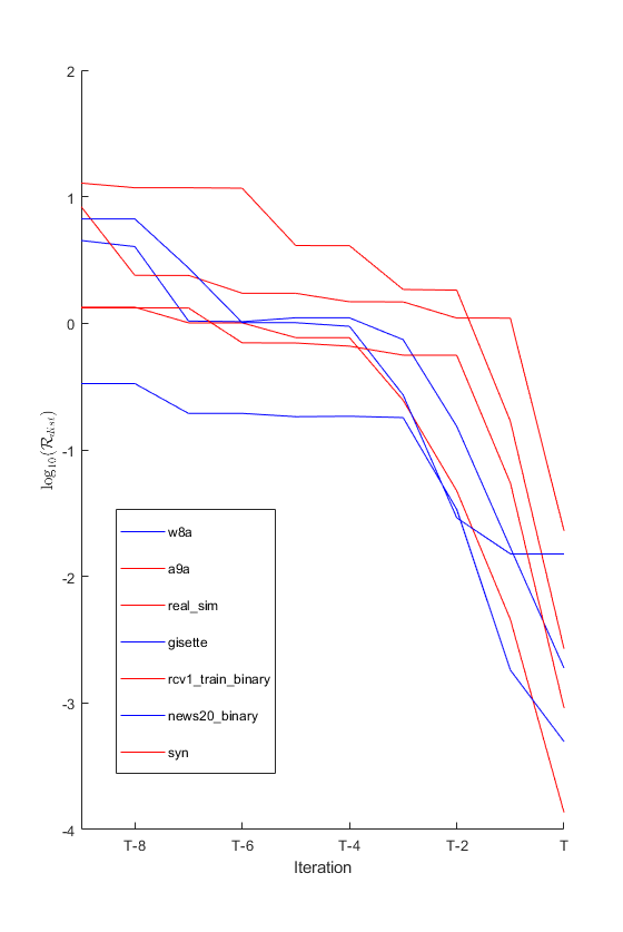
Figure 1: $\log_{10}{\cal R}_{opt}$ for the last ten iterations of SOIR$\ell_{1}$ applied to synthetic instances.

Figure 2: $\log_{10}{\cal R}_{dist}$ for the last ten iterations of SOIR$\ell_{1}$ applied to synthetic instances.

Real world datasets with $p=0.5$

Then we compare SOIR$\ell_{1}$ to the hybrid Newton method HpgSRN and the iteratively reweighted first-order method EPIR$\ell_{1}$ on real-world datasets. We use SOIR$\ell_{1}$-MN to denote the original algorithm Algorithm 1 and SOIR$\ell_{1}$-TR denotes the alternative local subproblem method discussed in Section 5.1. Initially, we standardize parameters across all datasets, setting $\lambda=1$ and $p=0.5$. Our primary focus is on evaluating performance based on CPU time, objective value and the percentage of zeros. To ensure accuracy, we repeat all experiments 10 times, taking the average of these values. For the second-order methods HpgSRN and SOIR$\ell_{1}$, the algorithm is terminated when ${\cal R}_{opt}$ decreases to $10^{-8}$ and $\|\bm{x}^{k}-\bm{x}^{k-1}\|/\|\bm{x}^{k}\|<10^{-9}$ (which is a straight inference for optimality measurement based on Proposition 1 and Lemma 4). For EPIR$\ell_{1}$, considering the trailing effect of first-order methods, we maintain its original termination condition of $\|\bm{x}^{k}-\bm{x}^{k-1}\|/\|\bm{x}^{k}\|<10^{-4}$ in addition to ${\cal R}_{opt}$. We limit EPIR$\ell_{1}$ to a maximum of 5000 iterations and all methods to a maximum time of 500 seconds. The performance of the three methods is shown in Table 3, with the best performance among the three methods highlighted in bold. Here we summarize the performance:

• In general, the second-order methods (SOIR$\ell_{1}$-MN, SOIR$\ell_{1}$-TR, HpgSRN) perform better than the first-order method (EPIR$\ell_{1}$) in terms of CPU time. SOIR$\ell_{1}$-TR requires the least CPU time on gisette and a9a while SOIR$\ell_{1}$-MN requires least on the rest. Compared to HpgSRN, our method consistently shows a marked advantage in computational speed.

• Our methods (SOIR$\ell_{1}$-MN, SOIR$\ell_{1}$-TR) always achieve the lowest or near-lowest objective values, suggesting effectiveness in minimizing the logistic regression problem. In some cases (e.g., w8a), while SOIR$\ell_{1}$ does not always achieve the absolute best objective value, it remains competitive with other algorithms.

• While maintaining low objective values, our methods (SOIR$\ell_{1}$-MN, SOIR$\ell_{1}$-TR) also maintain a sparsity similar to or better than the baseline (e.g., gisette).

Overall, our methods exhibit outstanding time efficiency across all datasets, often by significant margins, and produces a solution with superior objective function values and competitive sparsity.

Table 3: Performance comparison on real-world datasets with $\ell_{p}$-norm regularized logistic regression problem. All datasets are obtained from LIBSVM and the size of the feature matrix is enclosed in parentheses.

dataset	Algorithm	Time (s)	Objective	% of zeros
a9a	SOIR$\ell_{1}$-MN	0.5007	10579.4	45.53%
	SOIR$\ell_{1}$-TR	0.4194	10588.5	46.34%
(32561$\times$123)	HpgSRN	2.9001	10583.3	53.01%
	EPIR$\ell_{1}$	5.9884	10570.5	39.02%
w8a	SOIR$\ell_{1}$-MN	0.6145	5873.8	37.00%
	SOIR$\ell_{1}$-TR	1.3807	5876.9	37.00%
(49749$\times$300)	HpgSRN	2.0102	5856.5	37.00%
	EPIR$\ell_{1}$	13.0460	5865.1	38.00%
gisette	SOIR$\ell_{1}$-MN	35.0693	176.4	97.06%
	SOIR$\ell_{1}$-TR	32.7069	176.2	97.06%
(6000$\times$5000)	HpgSRN	36.5831	177.0	96.92%
	EPIR$\ell_{1}$	326.4776	178.3	97.02%
real sim	SOIR$\ell_{1}$-MN	3.8057	7121.6	93.63%
	SOIR$\ell_{1}$-TR	10.0057	7123.3	93.63%
(72309$\times$20958)	HpgSRN	6.8014	7262.3	94.47%
	EPIR$\ell_{1}$	33.4761	7152.7	93.78%
rcv1.train	SOIR$\ell_{1}$-MN	1.5928	2554.6	99.10%
	SOIR$\ell_{1}$-TR	3.9464	2558.9	99.08%
(20242$\times$47236)	HpgSRN	1.6934	2578.4	99.21%
	EPIR$\ell_{1}$	14.0964	2562.9	99.13%
news20	SOIR$\ell_{1}$-MN	20.0840	4034.5	99.97%
	SOIR$\ell_{1}$-TR	93.5413	3989.7	99.97%
(19996$\times$1355191)	HpgSRN	23.7392	4171.3	99.97%
	EPIR$\ell_{1}$	207.0546	3983.6	99.97%

Different $p$ value

The regularization problem with a small $\ell_{p}$-norm presents a more challenging task due to its stronger nonconvexity, compared to cases with larger $p$ values. To demonstrate our method’s superior performance, we conduct tests with $p=0.3$ on SOIR$\ell_{1}$-MN and HpgSRN for comparison. The problem settings and algorithm configurations were otherwise kept consistent.

For a clearer presentation of our findings, we have summarized the results for CPU times and objective values in Table 4. The CPU time and objective of SOIR$\ell_{1}$-MN are superior to HpgSRN, indicating a more pronounced advantage over HpgSRN compared to the $p=0.5$ scenario. Specifically, for datasets with large feature sizes like real-sim and news20, HpgSRN exhibits a significant increase in CPU time (7 times and 78 times, respectively), while our method performs similarly to the $p=0.5$ scenario. The reasons for this can be summarized as follows: (i) There is no analytical solution for the proximal mapping except for $p=0.5$ and $p=2/3$, so HpgSRN applies a numerical method for $p=0.3$ on the entire index set $\mathbb{R}^{n}$, while we only perform a soft thresholding step on a subset defined in line 13 or 10. (ii) From Theorem 4, we show that our method has a zero components detection scheme based on the $\bm{\epsilon}$ update strategy, which can quickly discard bad indices and force the method to enter the local phase.

Table 4: Comparison against HpgSRN with $p=0.3$.

	Dataset	news20	w8a	a9a	real sim	rcv1.train	gisette
SOIR$\ell_{1}$-MN	Time (s)	60.21	0.80	0.47	9.01	3.86	31.79
	Objective	3019.06	5825.87	10596.93	5669.32	1933.62	165.18
HpgSRN	Time (s)	1871.86	3.29	3.49	50.67	15.73	34.07
	Objective	3696.13	5802.88	10595.47	6099.26	2078.87	186.27

General nonconvex regularizers

To evaluate Algorithm 1 on a generic nonconvex regularization problem, we apply all approximation types listed in Table 1 to the $\ell_{p}$-norm logistic regression problem.

We use a9a as an illustrative example. To promote sparsity, we set $\lambda=1$ and use different values of $p$ for different regularizations. The performance is depicted in Figure 3, where we plot the logarithmic residuals across the last 10 iterations. The residual is defined as

$${\cal R}_{opt}=\|\bm{x}\circ(\nabla f(\bm{x})+\bm{\omega}(\bm{x},\bm{0})\circ\text{sign}(\bm{x}))\|_{\infty}.$$

which serves as an indicator of the optimal condition. Based on the data presented in Figure 3, it is evident that all methods successfully converge to a level of $10^{-8}$.

To further validate the effectiveness of our algorithm, we applied LOG regularization to a range of datasets. We set $p=10^{-2}$ for all datasets. The outcomes of these tests are compiled in Table 5. A straightforward comparison with the results from the $\ell_{p}$-norm regularized problem allows us to ascertain that Algorithm 1 effectively solves the LOG regularization problem across all datasets.

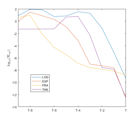
Figure 3: Experiments of four types of nonconvex regularization problem on synthetic dataset with $\lambda=1$. We set $p=10^{-3}$ for LOG, $p=0.05$ for EXP, FRA and $p=0.01$ for TAN.

Datasets	Time (s)	Objective	Sparsity
w8a	5.12	6580.04	53.67%
a9a	0.58	10762.03	64.23%
real sim	8.36	10357.00	96.54%
gisette	18.67	615.17	98.90%
news20	20.93	5488.77	99.98%
rcv1.train	1.34	5792.41	99.72%

Table 5: Experiments of LOG type nonconvex regularization problem on real datasets.

Conclusion

In this paper, we introduce a second-order iteratively reweighted $\ell_{1}$ method for a class of nonconvex sparsity-promoting regularization problems. Our approach, by reformulating nonconvex regularization into weighted $\ell_{1}$ form and incorporating subspace approximate Newton steps with subspace soft-thresholding steps, not only speeds up computation but also ensures algorithmic stability and convergence.

We prove global convergence under Lipschitz continuity and bounded Hessian conditions, achieving local superlinear convergence under KL property framework and local quadratic convergence with a strategic perturbation update. The method also extends to nonconvex and nonsmooth sparsity-driven regularization problems, maintaining similar convergence results. Empirical tests across various model prediction scenarios have demonstrated the method’s efficiency and effectiveness, suggesting its utility for complex optimization challenges in sparsity and nonconvexity contexts.

Appendix

Lemma 6.

Let $d(\mu)={\cal S}_{\mu\bm{\omega}}(\bm{x}-\mu g)-\bm{x}$ for $\mu>0$ where $\bm{x},g\in\mathbb{R}^{n}$ and $w\in\mathbb{R}^{n}_{++}$. It holds that

$$d_{i}(\mu) =\mu d_{i}(1) \text{ if }\ x_{i}=0,$$ (1)

$$|d_{i}(\mu)| \geq\min\{\mu,1\}|d_{i}(1)| \text{ if }\ x_{i}\neq 0.$$ (2)

Moreover, for $\omega_{i}>|g_{i}-x_{i}|$, $d_{i}(\mu)=-x_{i}$.

Proof.

It holds from the soft-thresholding operator that

$$d_{i}(\mu)=\begin{cases}-\mu(g_{i}+\omega_{i}),&\text{if }\mu(g_{i}+\omega_{i})<\bm{x}_{i},\\ -\mu(g_{i}-\omega_{i}),&\text{if }\mu(g_{i}-\omega_{i})>\bm{x}_{i},\\ -\bm{x}_{i},&\text{otherwise.}\end{cases}$$ (3)

If $i\in{\cal I}_{0}(\bm{x})$, $x_{i}=0$. It is obvious that $d_{i}(\mu)=-\mu d_{i}(1)$.

If $i\in{\cal I}(\bm{x})$, $x_{i}\neq 0$. We check the values of $d_{i}(1)$.

If $d_{i}(1)=-(g_{i}+\omega_{i})$, which means

$$g_{i}+\omega_{i}<x_{i}$$ (4)

by the expression of $d_{i}(1)$, we consider the order of $x_{i},\mu(g_{i}+\omega_{i}),\mu(g_{i}-\omega_{i})$.

Case (a): $\mu(g_{i}-\omega_{i})<\mu(g_{i}+\omega_{i})<\bm{x}_{i}$, this belongs to the first case in $d_{i}(\mu)$, meaning $d_{i}(\mu)=-\mu d_{i}(1)$.

Case (b): $\mu(g_{i}-\omega_{i})\leq\bm{x}_{i}\leq\mu(g_{i}+\omega_{i})$, this belongs to the third case in $d_{i}(\mu)$, so that $d_{i}(\mu)=-x_{i}$. It follows from (4) that

$$g_{i}+\omega_{i}<x_{i}<\mu(g_{i}+\omega_{i}),$$ (5)

meaning $0<g_{i}+\omega_{i}<x_{i},\mu>x_{i}/(g_{i}+\omega_{i})>1$ or $g_{i}+\omega_{i}<x_{i}<0,\mu<x_{i}/(g_{i}+\omega_{i})<1$ by noticing (4). In either case, $|x_{i}|>\min(\mu,1)|g_{i}+\omega_{i}|$, meaning $|d_{i}(\mu)|>\min(\mu,1)|d_{i}(1)|$.

Case (c): $\bm{x}_{i}<\mu(g_{i}-\omega_{i})<\mu(g_{i}+\omega_{i})$, this belongs to the second case in $d_{i}(\mu)$, so that $d_{i}(\mu)=-\mu(g_{i}-\omega_{i})$. It follows from (4) that

$$g_{i}+\omega_{i}<\mu(g_{i}-\omega_{i})<\mu(g_{i}+\omega_{i}),$$ (6)

meaning $\nabla_{i}f(\bm{x})+\omega_{i}>0,\mu>1$ or $\nabla_{i}f(\bm{x})+\omega_{i}<0,\mu<1$. In either case, (6) implies that $|\mu(g_{i}-\omega_{i})|>\min(\mu,1)|g_{i}+\omega_{i}|$, indicating $|d_{i}(\mu)|>\min(\mu,1)|d_{i}(1)|$.

If $d_{i}(1)=-(g_{i}-\omega_{i})$, this means $g_{i}+\omega_{i}<x_{i}$. same argument based on the order of we consider the order of $x_{i},\mu(g_{i}+\omega_{i}),\mu(g_{i}-\omega_{i})$ also yields (2)

If $d_{i}(1)=-x_{i}$, this means $g_{i}+\omega_{i}>x_{i}>g_{i}-\omega_{i}$, the same argument based on the order of we consider the order of $x_{i},\mu(g_{i}+\omega_{i}),\mu(g_{i}-\omega_{i})$ also yields (2). ∎

6.3 Proof of Theorem 8

Proof.

The proof follow exactly [18, Theorem 10]. For completeness, we provide the following arguments. By the monotonicity of $\{F(\bm{x}^{k},\bm{\epsilon}^{k})\},k>\hat{k}$, there exist a constant $\nu$ such that $\nu=\lim_{k\to\infty}F(\bm{x}^{k},\bm{\epsilon}^{k})=F(\bm{x}^{*},0)$.

Since $F$ has the KL property at all stationary point $(\bm{x}^{*},0)$, the KL inequality implies that for all $k>\bar{k}$,

$$\phi^{{}^{\prime}}(F(\bm{x}^{k},\bm{\varepsilon}^{k})-\nu)\|\nabla F(\bm{x}^{k},\bm{\varepsilon}^{k})\|\geq 1.$$ (7)

It follows that for any $k>\bar{k}$,

$$[\phi(F(\bm{x}^{k},\bm{\varepsilon}^{k})-\nu)-\phi(F(\bm{x}^{k+1},\bm{\varepsilon}^{k+1})-\nu)]\cdot C_{2}(\|\bm{x}^{k+1}-\bm{x}^{k}\|+\|\bm{\varepsilon}^{k}\|_{1}-\|\bm{\varepsilon}^{k+1}\|_{1})$$ (8)

$$\geq [\phi(F(\bm{x}^{k},\bm{\varepsilon}^{k})-\nu)-\phi(F(\bm{x}^{k+1},\bm{\varepsilon}^{k+1})-\nu)]\cdot\|\nabla F(\bm{x}^{k},\bm{\varepsilon}^{k})\|$$

$$\geq \phi^{{}^{\prime}}(F(\bm{x}^{k},\bm{\varepsilon}^{k})-\nu)\cdot[F(\bm{x}^{k},\bm{\varepsilon}^{k})-F(\bm{x}^{k+1},\bm{\varepsilon}^{k+1})]\cdot\|\nabla F(\bm{x}^{k},\bm{\varepsilon}^{k})\|$$

$$\geq F(\bm{x}^{k},\bm{\varepsilon}^{k})-F(\bm{x}^{k+1},\bm{\varepsilon}^{k+1})$$

$$\geq C_{1}\|\bm{x}^{k+1}-\bm{x}^{k}\|^{2},$$

where the first inequality is by (44), the second inequality is by the concavity of $\phi$, and the third inequality is by (7) and the last inequality is by (38). Rearranging and taking the square root of both sides, and using the inequality of arithmetic and geometric means inequality, we have

$$\|\bm{x}^{k+1}-\bm{x}^{k}\|\leq \sqrt{\frac{2C_{2}}{C_{1}}[\phi(F(\bm{x}^{k},\bm{\varepsilon}^{k})-\nu)-\phi(F(\bm{x}^{k+1},\bm{\varepsilon}^{k+1})-\nu)]}$$ (9)

$$\times\sqrt{\frac{1}{2}\|\bm{x}^{k+1}-\bm{x}^{k}\|+\|\bm{\varepsilon}^{k}\|_{1}-\|\bm{\varepsilon}^{k+1}\|_{1}}$$

$$\leq \frac{C_{2}}{C_{1}}[\phi(F(\bm{x}^{k},\bm{\varepsilon}^{k})-\nu)-\phi(F(\bm{x}^{k+1},\bm{\varepsilon}^{k+1})-\nu)]$$

$$+\frac{1}{4}[\|\bm{x}^{k+1}-\bm{x}^{k}\|+\|\bm{\varepsilon}^{k}\|_{1}-\|\bm{\varepsilon}^{k+1}\|_{1}]$$

Subtracting $\frac{1}{4}\|(\bm{x}^{k+1},\bm{\varepsilon}^{k+1})-(\bm{x}^{k},\bm{\varepsilon}^{k})\|$ from both sides, we have

$$\frac{3}{4}\|\bm{x}^{k+1}-\bm{x}^{k}\|\leq \frac{C_{2}}{C_{1}}[\phi(F(\bm{x}^{k},\bm{\varepsilon}^{k})-\nu)-\phi(F(\bm{x}^{k+1},\bm{\varepsilon}^{k+1})-\nu)$$

$$+\frac{1}{4}[\|\bm{x}^{k+1}-\bm{x}^{k}\|-\|\bm{x}^{k+1}-\bm{x}^{k}\|+\|\bm{\varepsilon}^{k}\|_{1}-\|\bm{\varepsilon}^{k+1}\|_{1}]$$

Summing up both side from $\bar{k}$ to $t$, we have

$$\frac{3}{4}\sum_{k=\bar{k}}^{t}\|\bm{x}^{k+1}-\bm{x}^{k}\|\leq \frac{C_{2}}{C_{1}}[\phi(F(\bm{x}^{\bar{k}},\bm{\varepsilon}^{\bar{k}})-\nu)-\phi(F(\bm{x}^{t+1},\bm{\varepsilon}^{t+1})-\nu)]$$ (10)

$$+\frac{1}{4}[\|\bm{x}^{\bar{k}}-\bm{x}^{\bar{k}-1}\|-\|\bm{x}^{t+1}-\bm{x}^{t}\|+\|\bm{\varepsilon}^{\bar{k}-1}\|_{1}-\|\bm{\varepsilon}^{t}\|_{1}]$$

Now letting $t\to\infty$, we know that $\|\bm{\varepsilon}^{t}\|_{1}\to 0$, $\|\bm{x}^{t+1}-\bm{x}^{t}\|\to 0$, $\phi(F(\bm{x}^{t+1},\bm{\varepsilon}^{t+1})-\nu)\to\phi(\nu-\nu)=0$. Therefore, we have

$$\sum_{k=\bar{k}}^{\infty}\|\bm{x}^{k+1}-\bm{x}^{k}\|\leq\frac{4C_{2}}{3C_{1}}\phi(F(\bm{x}^{\bar{k}},\bm{\varepsilon}^{\bar{k}})-\nu)+\frac{1}{3}(\|\bm{x}^{\bar{k}}-\bm{x}^{\bar{k}-1}\|+\|\bm{\varepsilon}^{\bar{k}-1}\|_{1})<\infty.$$ (11)

Hence $\{\bm{x}^{k}\}$ is a Cauchy sequence, and consequently, it is a convergent sequence

(i) If $\theta=0$, then $\phi(s)=cs$, $\phi^{{}^{\prime}}(s)\equiv c$. We claim that there must exist $k_{0}>0$ such that $F(\bm{x}^{k},\bm{\varepsilon}^{k})=\nu$. Suppose by contradiction that $F(z^{k})>\nu$ for all $k$. The KL inequality implies that for all sufficiently large k,

$$c\|\nabla F(\bm{x}^{k},\bm{\varepsilon}^{k})\|_{2}\geq 1,$$

contradicting $\|\nabla F(\bm{x}^{k},\bm{\varepsilon}^{k})\|\to 0$ by Corollary 1. Therefore, there exists $k_{0}\in\mathbb{N}$ so that $F(\bm{x}^{k},\bm{\varepsilon}^{k})=F(\bm{x}^{k_{0}},\bm{\varepsilon}^{k_{0}})=\nu$ for any $k>k_{0}$. Hence, we conclude from (38) that $\bm{x}^{k+1}=\bm{x}^{k}$ for all $k>k_{0}$, meaning $\bm{x}^{k}\equiv\bm{x}^{*}=\bm{x}^{k_{0}}$ for all $k>k_{0}$.

(ii)-(iii) Next consider $\theta\in(0,1)$. First of all, if there exist $k_{0}\in\mathbb{N}$ such that $F(\bm{x}^{k_{0}},\bm{\varepsilon}^{k_{0}})=\nu$, then by the monotonicity of $\{F(\bm{x}^{k},\bm{\epsilon}^{k})\}$ we can see that $\{\bm{x}^{k}\}$ converges finitely. Thus, we only need to consider the case that $F(\bm{x}^{k},\bm{\epsilon}^{k})>\nu$ for all $k$.

Define $S^{k}=\sum_{l=k}^{\infty}\|\bm{x}^{l+1}-\bm{x}^{l}\|_{2}$. It holds that

$$\|\bm{x}^{k}-\bm{x}^{*}\|_{2}=\|\bm{x}^{k}-\lim_{t\to\infty}\bm{x}^{t}\|=\|\lim_{t\to\infty}\sum_{l=k}^{t}(\bm{x}^{l+1}-\bm{x}^{l})\|_{2}\leq\sum_{l=k}^{\infty}\|\bm{x}^{l+1}-\bm{x}^{l}\|_{2}=S^{k}.$$

Therefore, we only have to prove $S^{k}$ also has the same upper bound as in Equation 36 and Equation 37. To derive the upper bound for $S^{k}$, by KL inequality with $\phi^{{}^{\prime}}(s)=c(1-s)s^{-\theta}$, for $k>\bar{k}$,

$$c(1-\theta)(F(\bm{x}^{k},\bm{\varepsilon}^{k})-\nu)^{-\theta}\|\nabla F(\bm{x}^{k},\bm{\varepsilon}^{k})\|_{2}\geq 1.$$ (12)

On the other hand, using (44) and the definition of $S^{k}$, we see that for all sufficiently large $k$,

$$\|\nabla F(\bm{x}^{k},\bm{\varepsilon}^{k})\|\leq C_{2}(S^{k-1}-S^{k}++\|\bm{\varepsilon}^{k-1}\|_{1}-\|\bm{\varepsilon}^{k}\|_{1}))$$

Combining with (12), we have

$$(F(\bm{x}^{k},\bm{\varepsilon}^{k})-\nu)^{\theta}\leq C_{2}c(1-\theta)(S^{k-1}-S^{k}++\|\bm{\varepsilon}^{k-1}\|_{1}-\|\bm{\varepsilon}^{k}\|_{1}))$$

Taking a power of $(1-\theta)/\theta$ to both sides of the above inequality and scaling both sides by $c$, we obtain that for all $k>\bar{k}$

$$\phi(F(\bm{x}^{k},\bm{\varepsilon}^{k})-\nu) =c(F(\bm{x}^{k},\bm{\varepsilon}^{k})-\nu)^{1-\theta}$$ (13)

$$\leq c[C_{2}c(1-\theta)(S^{k-1}-S^{k}++\|\bm{\varepsilon}^{k-1}\|_{1}-\|\bm{\varepsilon}^{k}\|_{1})]^{\frac{1-\theta}{\theta}}$$

$$\leq c[C_{2}c(1-\theta)(S^{k-1}-S^{k}+\|\bm{\varepsilon}^{k-1}\|)]^{\frac{1-\theta}{\theta}}$$

From (11), we have

$$S^{k}\leq\frac{4C_{2}}{3C_{1}}\phi(F(\bm{x}^{k},\bm{\varepsilon}^{k})-\nu)+\frac{1}{3}(\|\bm{x}^{k}-\bm{x}^{k-1}\|+\|\bm{\varepsilon}^{k-1}\|_{1}).$$ (14)

Combing (13) and (14), we have

$$S^{k} \leq C_{3}[(S^{k-1}-S^{k}+\|\bm{\varepsilon}^{k-1}\|)]^{\frac{1-\theta}{\theta}}+\frac{1}{3}[S^{k-1}-S^{k}+\|\bm{\varepsilon}^{k-1}\|_{1}]$$ (15)

$$\leq C_{3}[(S^{k-2}-S^{k}+\|\bm{\varepsilon}^{k-1}\|)]^{\frac{1-\theta}{\theta}}+\frac{1}{3}[S^{k-2}-S^{k}+\|\bm{\varepsilon}^{k-1}\|_{1}]$$

where $C_{3}:=\frac{4C_{2}c}{3C_{1}}[C_{2}\cdot c(1-\theta)]^{\frac{1-\theta}{\theta}}$. It follows that

$$S^{k}+\frac{\sqrt{\beta}}{1-\beta}\|\bm{\varepsilon}^{k}\|_{1}$$ (16)

$$\leq C_{3}[(S^{k-2}-S^{k}+\|\bm{\varepsilon}^{k-1}\|)]^{\frac{1-\theta}{\theta}}+\frac{1}{3}[S^{k-2}-S^{k}+\|\bm{\varepsilon}^{k-1}\|_{1}]+\frac{\sqrt{\beta}}{1-\beta}\|\bm{\varepsilon}^{k}\|_{1}$$

$$\leq C_{3}[(S^{k-2}-S^{k}+\|\bm{\varepsilon}^{k-1}\|)]^{\frac{1-\theta}{\theta}}+\frac{1}{3}[S^{k-2}-S^{k}+\|\bm{\varepsilon}^{k-1}\|_{1}]+\frac{\beta}{1-\beta}\|\bm{\varepsilon}^{k}\|_{1}$$

$$\leq C_{3}[(S^{k-2}-S^{k}+\|\bm{\varepsilon}^{k-1}\|)]^{\frac{1-\theta}{\theta}}+C_{4}[S^{k-2}-S^{k}+\|\bm{\varepsilon}^{k-1}\|_{1}]$$

with $C_{4}:=\frac{1}{3}+\frac{\beta}{1-\beta}$ and the second inequality is by the update $\bm{\varepsilon}^{k}\leq\sqrt{\beta}\bm{\varepsilon}^{k-1}$.

For part (ii), $\theta\in(0,\frac{1}{2}]$. Notice that

$$\frac{1-\theta}{\theta}\geq 1\text{ and }(S^{k-2}-S^{k}+\|\bm{\varepsilon}^{k-1}\|_{1})\to 0.$$

Hence, there exists sufficient large $k$ such that

$$(S^{k-2}-S^{k}+\|\bm{\varepsilon}^{k-1}\|_{1})^{\frac{1-\theta}{\theta}}\leq S^{k-2}-S^{k}+\|\bm{\varepsilon}^{k-1}\|_{1}$$

we assume the above inequality holds for all $k\geq\bar{k}$. This, combined with (15), yields

$$S^{k}+\frac{\sqrt{\beta}}{1-\beta}\|\bm{\varepsilon}^{k}\|_{1}\leq(C_{3}+C_{4})(S^{k-2}-S^{k}+\|\bm{\varepsilon}^{k-1}\|_{1})$$ (17)

for any $k>\bar{k}$. Using $\varepsilon_{i}^{k}\leq\beta\varepsilon_{i}^{k-1}$, we can show that

$$\varepsilon_{i}^{k-1}\leq\frac{\sqrt{\beta}}{1-\beta}(\varepsilon_{i}^{k-2}-\varepsilon_{i}^{k}).$$ (18)

Combining (17) and (18) gives

$$S^{k}+\frac{\sqrt{\beta}}{1-\beta}\|\bm{\varepsilon}^{k}\|_{1}\leq(C_{3}+C_{4})[(S^{k-2}+\frac{\sqrt{\beta}}{1-\beta}\|\bm{\varepsilon}^{k-2}\|_{1})-(S^{k}+\frac{\sqrt{\beta}}{1-\beta}\|\bm{\varepsilon}^{k}\|_{1})]$$

Rearranging this inequality gives

$$S^{k}+\frac{\sqrt{\beta}}{1-\beta}\|\bm{\varepsilon}^{k}\|_{1} \leq\frac{C_{3}+C_{4}}{1+C_{3}+C_{4}}(S^{k-2}+\frac{\sqrt{\beta}}{1-\beta}\|\bm{\varepsilon}^{k-2}\|_{1})$$

$$\leq(\frac{C_{3}+C_{4}}{1+C_{3}+C_{4}})^{\lfloor\frac{k}{2}\rfloor}(S^{k\text{ mod }2}+\frac{\sqrt{\beta}}{1-\beta}\|\bm{\varepsilon}^{k\text{ mod }2}\|_{1})$$

$$\leq(\frac{C_{3}+C_{4}}{1+C_{3}+C_{4}})^{\frac{k-1}{2}}(S^{0}+\frac{\sqrt{\beta}}{1-\beta}\|\bm{\varepsilon}^{0}\|_{1})$$

Therefore, for any $k>\bar{k}$,

$$\|\bm{x}^{k}-\bm{x}^{*}\|\leq S^{k}+\frac{\sqrt{\beta}}{1-\beta}\|\bm{\varepsilon}^{k}\|_{1}\leq c_{1}\gamma^{k}$$

with

$$c_{1}=(\frac{C_{3}+C_{4}}{1+C_{3}+C_{4}})^{-\frac{1}{2}}(S^{0}+\frac{\sqrt{\beta}}{1-\beta}\|\bm{\varepsilon}^{0}\|)\text{ and }\gamma=(\frac{C_{3}+C_{4}}{1+C_{3}+C_{4}})^{\frac{1}{2}}.$$

which completes the proof of (ii).

For part (iii), $\theta\in(\frac{1}{2},1)$. Notice that

$$\frac{1-\theta}{\theta}\leq 1\text{ and }(S^{k-2}-S^{k}+\|\bm{\varepsilon}^{k-1}\|_{1})\to 0.$$

Hence, there exists sufficient large $k$ such that

$$(S^{k-2}-S^{k}+\|\bm{\varepsilon}^{k-1}\|)^{\frac{1-\theta}{\theta}}\geq S^{k-2}-S^{k}+\|\bm{\varepsilon}^{k-1}\|$$

we assume the above inequality holds for all $k\geq\bar{k}$. This, combined with (15), yields

$$S^{k}+\frac{\sqrt{\beta}}{1-\beta}\|\bm{\varepsilon}^{k}\|_{1} \leq(C_{3}+C_{4}))(S^{k-2}-S^{k}+\|\bm{\varepsilon}^{k-1}\|_{1})^{\frac{1-\theta}{\theta}}$$

This combined with (18), yields

$$S^{k}+\frac{\sqrt{\beta}}{1-\beta}\|\bm{\varepsilon}^{k}\|_{1}\leq(C_{3}+C_{4})[(S^{k-2}+\frac{\sqrt{\beta}}{1-\beta}\|\bm{\varepsilon}^{k-2}\|_{1})-(S^{k}+\frac{\sqrt{\beta}}{1-\beta}\|\bm{\varepsilon}^{k}\|_{1})]^{\frac{1-\theta}{\theta}}$$

Raising to a power of $\frac{\theta}{1-\theta}$ of both sides of the above inequality, we see

$$[S^{k}+\frac{\sqrt{\beta}}{1-\beta}\|\bm{\varepsilon}^{k}\|_{1}]^{\frac{\theta}{1-\theta}}\leq C_{5}[(S^{k-2}+\frac{\sqrt{\beta}}{1-\beta}\|\bm{\varepsilon}^{k-2}\|_{1})-(S^{k}+\frac{\sqrt{\beta}}{1-\beta}\|\bm{\varepsilon}^{k}\|_{1})]$$ (19)

where $C_{5}:=(C_{3}+C_{4})^{\frac{\theta}{1-\theta}}$. Consider the ”even” subsequence of $\{\bar{k},\bar{k}+1\}$ and define $\{\Delta_{t}\}_{t\geq N_{1}}$ with $N_{1}:=\lceil\bar{k}/2\rceil$, and $\Delta_{t}:=S^{2t}+\frac{\sqrt{\beta}}{1-\beta}\|\bm{\varepsilon}^{2t}\|_{1}$. Then for all $t>N_{1}$, we have

$$\Delta_{t}^{\frac{\theta}{1-\theta}}\leq C_{5}(\Delta_{t-1}-\Delta_{t})$$ (20)

The remaining part of our proof is similar to ([18] Theorem 10, [47] Theorem 2). Define $h:(0,+\infty)\rightarrow\mathbb{R}$ by $h(s)=s^{-\frac{\theta}{1-\theta}}$ and let $T\in(1,+\infty)$. Take $k\geq N_{1}$ and consider the case that $h\left(\Delta_{k}\right)\leq Th\left(\Delta_{k-1}\right)$ holds. By rewriting (20) as

$$1\leq C_{5}\left(\Delta_{k-1}-\Delta_{k}\right)\Delta_{k}^{-\frac{\theta}{1-\theta}}$$

we obtain that

$$1 \leq C_{5}\left(\Delta_{k-1}-\Delta_{k}\right)h\left(\Delta_{k}\right)$$

$$\leq TC_{5}\left(\Delta_{k-1}-\Delta_{k}\right)h\left(\Delta_{k-1}\right)$$

$$\leq TC_{5}\int_{\Delta_{k}}^{\Delta_{k-1}}h(s)ds$$

$$\leq TC_{5}\frac{1-\theta}{1-2\theta}\left[\Delta_{k-1}^{\frac{1-2\theta}{1-\theta}}-\Delta_{k}^{\frac{1-2\theta}{1-\theta}}\right]$$

Thus if we set $u=\frac{2\theta-1}{(1-\theta)TC_{5}}>0$ and $\sigma=\frac{1-2\theta}{1-\theta}<0$ one obtains that

$$0<u\leq\Delta_{k}^{\sigma}-\Delta_{k-1}^{\sigma}$$ (21)

Assume now that $h\left(\Delta_{k}\right)>Th\left(\Delta_{k}\right)$ and set $q=\left(\frac{1}{T}\right)^{\frac{1-\theta}{\theta}}\in(0,1)$. It follows immediately that $\Delta_{k}\leq q\Delta_{k-1}$ and furthermore - recalling that $\sigma$ is negative - we have

$$\Delta_{k}^{\sigma}\geq q^{\sigma}\Delta_{k-1}^{\sigma}\quad\text{ and }\quad\Delta_{k}^{\sigma}-\Delta_{k-1}^{\sigma}\geq\left(q^{\sigma}-1\right)\Delta_{k-1}^{\sigma}.$$

Since $q^{\sigma}-1>0$ and $\Delta_{t}\rightarrow 0^{+}$as $t\rightarrow+\infty$, there exists $\bar{u}>0$ such that $\left(q^{\sigma}-1\right)\Delta_{t-1}^{\sigma}>\bar{u}$ for all $t\geq N_{1}$. Therefore we obtain that

$$\Delta_{k}^{\nu}-\Delta_{k-1}^{\nu}\geq\bar{u}$$ (22)

If we set $\hat{u}=\min\{u,\bar{u}\}>0$, one can combine (21) and (22) to obtain that

$$\Delta_{k}^{\nu}-\Delta_{k-1}^{\nu}\geq\hat{u}>0$$

for all $k\geq N_{1}$. By summing those inequalities from $N_{1}$ to some $t$ greater than $N_{1}$ we obtain that $\Delta_{t}^{\nu}-\Delta_{N_{1}}^{\nu}\geq\hat{u}\left(t-N_{1}\right)$, implying

$$\Delta_{t}\leq\left[\Delta_{N_{1}}^{\nu}+\hat{u}\left(t-N_{1}\right)\right]^{1/\nu}\leq C_{6}t^{-\frac{1-\theta}{2\theta-1}}$$ (23)

for some $C_{6}>0$.

As for the ”odd” subsequence of $\{\bar{k},\bar{k}+1,\ldots\}$, we can define $\left\{\Delta_{t}\right\}_{t\geq\lceil\bar{k}/2\rceil}$ with $\Delta_{t}:=S^{2t+1}+$ $\frac{\sqrt{\mu}}{1-\mu}\left\|\bm{\varepsilon}^{2t+1}\right\|_{1}$ and then can still show that (23) holds true.

Therefore, for all sufficiently large and even number $k$,

$$\left\|\bm{x}^{k}-\bm{x}^{*}\right\|_{2}\leq\Delta_{\frac{k}{2}}\leq 2^{\frac{1-\theta}{2\theta-1}}C_{6}k^{-\frac{1-\theta}{2\theta-1}}$$

For all sufficiently large and odd number $k$, there exists $C_{7}>0$ such that

$$\left\|\bm{x}^{k}-\bm{x}^{*}\right\|_{2}\leq\Delta_{\frac{k-1}{2}}\leq 2^{\frac{1-\theta}{2\theta-1}}C_{6}(k-1)^{-\frac{1-\theta}{2\theta-1}}\leq 2^{\frac{1-\theta}{2\theta-1}}C_{7}k^{-\frac{1-\theta}{2\theta-1}}$$

Overall, we have

$$\left\|\bm{x}^{k}-\bm{x}^{*}\right\|_{2}\leq c_{2}k^{-\frac{1-\theta}{2\theta-1}}$$

where

$$c_{2}:=2^{\frac{1-\theta}{2\theta-1}}\max\left(C_{6},C_{7}\right).$$

This completes the proof of (iii). ∎

References

- \bibcommenthead
- Zhang [2010] Zhang, C.-H.: Nearly unbiased variable selection under minimax concave penalty. The Annals of Statistics 38(2), 894–942 (2010)
- Fan and Li [2001] Fan, J., Li, R.: Variable selection via nonconcave penalized likelihood and its oracle properties. Journal of the American Statistical Association 96(456), 1348–1360 (2001)
- Zhang [2010] Zhang, T.: Analysis of multi-stage convex relaxation for sparse regularization. Journal of Machine Learning Research 11(3) (2010)
- Wu and Lange [2008] Wu, T.T., Lange, K.: Coordinate descent algorithms for lasso penalized regression (2008)
- Wright et al. [2009] Wright, S.J., Nowak, R.D., Figueiredo, M.A.: Sparse reconstruction by separable approximation. IEEE Transactions on signal processing 57(7), 2479–2493 (2009)
- Beck and Teboulle [2009] Beck, A., Teboulle, M.: A fast iterative shrinkage-thresholding algorithm for linear inverse problems. SIAM journal on imaging sciences 2(1), 183–202 (2009)
- Chen et al. [2017] Chen, T., Curtis, F.E., Robinson, D.P.: A reduced-space algorithm for minimizing -regularized convex functions. SIAM Journal on Optimization 27(3), 1583–1610 (2017)
- Byrd et al. [2016] Byrd, R.H., Nocedal, J., Oztoprak, F.: An inexact successive quadratic approximation method for l-1 regularized optimization. Mathematical Programming 157(2), 375–396 (2016)
- Yuan et al. [2011] Yuan, G.-X., Ho, C.-H., Lin, C.-J.: An improved glmnet for l1-regularized logistic regression. In: Proceedings of the 17th ACM SIGKDD International Conference on Knowledge Discovery and Data Mining, pp. 33–41 (2011)
- Hu et al. [2017] Hu, Y., Li, C., Meng, K., Qin, J., Yang, X.: Group sparse optimization via regularization. The Journal of Machine Learning Research 18(1), 960–1011 (2017)
- Ge et al. [2011] Ge, D., Jiang, X., Ye, Y.: A note on the complexity of minimization. Mathematical programming 129, 285–299 (2011)
- Gazzola et al. [2021] Gazzola, S., Nagy, J.G., Landman, M.S.: Iteratively reweighted fgmres and flsqr for sparse reconstruction. SIAM Journal on Scientific Computing 43(5), 47–69 (2021)
- Zhou et al. [2021] Zhou, X., Liu, X., Wang, C., Zhai, D., Jiang, J., Ji, X.: Learning with noisy labels via sparse regularization. In: Proceedings of the IEEE/CVF International Conference on Computer Vision, pp. 72–81 (2021)
- Liu et al. [2007] Liu, Z., Jiang, F., Tian, G., Wang, S., Sato, F., Meltzer, S.J., Tan, M.: Sparse logistic regression with lp penalty for biomarker identification. Statistical Applications in Genetics and Molecular Biology 6(1) (2007)
- Candes et al. [2008] Candes, E.J., Wakin, M.B., Boyd, S.P.: Enhancing sparsity by reweighted minimization. Journal of Fourier analysis and applications 14, 877–905 (2008)
- Lu [2014] Lu, Z.: Iterative reweighted minimization methods for regularized unconstrained nonlinear programming. Mathematical Programming 147(1-2), 277–307 (2014)
- Wang et al. [2021] Wang, H., Zeng, H., Wang, J., Wu, Q.: Relating regularization and reweighted regularization. Optimization Letters 15(8), 2639–2660 (2021)
- Wang et al. [2023] Wang, H., Zeng, H., Wang, J.: Convergence rate analysis of proximal iteratively reweighted methods for regularization problems. Optimization Letters 17(2), 413–435 (2023)
- Wang et al. [2022] Wang, H., Zeng, H., Wang, J.: An extrapolated iteratively reweighted method with complexity analysis. Computational Optimization and Applications 83(3), 967–997 (2022)
- Lai et al. [2013] Lai, M.-J., Xu, Y., Yin, W.: Improved iteratively reweighted least squares for unconstrained smoothed minimization. SIAM Journal on Numerical Analysis 51(2), 927–957 (2013)
- Chen et al. [2013] Chen, X., Niu, L., Yuan, Y.: Optimality conditions and a smoothing trust region newton method for nonlipschitz optimization. SIAM Journal on Optimization 23(3), 1528–1552 (2013)
- Chen and Zhou [2014] Chen, X., Zhou, W.: Convergence of the reweighted minimization algorithm for minimization. Computational Optimization and Applications 59(1-2), 47–61 (2014)
- Chen and Zhou [2010] Chen, X., Zhou, W.: Convergence of reweighted minimization algorithms and unique solution of truncated minimization. Department of Applied Mathematics, The Hong Kong Polytechnic University (2010)
- Xu et al. [2012] Xu, Z., Chang, X., Xu, F., Zhang, H.: regularization: A thresholding representation theory and a fast solver. IEEE Transactions on neural networks and learning systems 23(7), 1013–1027 (2012)
- Lai and Wang [2011] Lai, M.-J., Wang, J.: An unconstrained minimization with for sparse solution of underdetermined linear systems. SIAM Journal on Optimization 21(1), 82–101 (2011)
- Yu and Pong [2019] Yu, P., Pong, T.K.: Iteratively reweighted algorithms with extrapolation. Computational Optimization and Applications 73(2), 353–386 (2019)
- Chen et al. [2016] Chen, F., Shen, L., Suter, B.W.: Computing the proximity operator of the norm with . IET Signal Processing 10(5), 557–565 (2016)
- Liu and Lin [2024] Liu, Y., Lin, R.: A bisection method for computing the proximal operator of the -norm for any with application to schatten p-norms. Journal of Computational and Applied Mathematics 447, 115897 (2024)
- Hu et al. [2021] Hu, Y., Li, C., Meng, K., Yang, X.: Linear convergence of inexact descent method and inexact proximal gradient algorithms for lower-order regularization problems. Journal of Global Optimization 79(4), 853–883 (2021)
- Lee et al. [2014] Lee, J.D., Sun, Y., Saunders, M.A.: Proximal newton-type methods for minimizing composite functions. SIAM Journal on Optimization 24(3), 1420–1443 (2014)
- Yue et al. [2019] Yue, M.-C., Zhou, Z., So, A.M.-C.: A family of inexact sqa methods for non-smooth convex minimization with provable convergence guarantees based on the luo–tseng error bound property. Mathematical Programming 174(1), 327–358 (2019)
- Mordukhovich et al. [2023] Mordukhovich, B.S., Yuan, X., Zeng, S., Zhang, J.: A globally convergent proximal newton-type method in nonsmooth convex optimization. Mathematical Programming 198(1), 899–936 (2023)
- Liu et al. [2024] Liu, R., Pan, S., Wu, Y., Yang, X.: An inexact regularized proximal newton method for nonconvex and nonsmooth optimization. Computational Optimization and Applications, 1–39 (2024)
- Burke and Moré [1988] Burke, J.V., Moré, J.J.: On the identification of active constraints. SIAM Journal on Numerical Analysis 25(5), 1197–1211 (1988)
- Liang et al. [2017] Liang, J., Fadili, J., Peyré, G.: Activity identification and local linear convergence of forward–backward-type methods. SIAM Journal on Optimization 27(1), 408–437 (2017)
- Sun et al. [2019] Sun, Y., Jeong, H., Nutini, J., Schmidt, M.: Are we there yet? manifold identification of gradient-related proximal methods. In: The 22nd International Conference on Artificial Intelligence and Statistics, pp. 1110–1119 (2019). PMLR
- Themelis et al. [2018] Themelis, A., Stella, L., Patrinos, P.: Forward-backward envelope for the sum of two nonconvex functions: Further properties and nonmonotone linesearch algorithms. SIAM Journal on Optimization 28(3), 2274–2303 (2018)
- Themelis et al. [2019] Themelis, A., Ahookhosh, M., Patrinos, P.: On the acceleration of forward-backward splitting via an inexact newton method. Splitting Algorithms, Modern Operator Theory, and Applications, 363–412 (2019)
- Bareilles et al. [2023] Bareilles, G., Iutzeler, F., Malick, J.: Newton acceleration on manifolds identified by proximal gradient methods. Mathematical Programming 200(1), 37–70 (2023)
- Wu et al. [2022] Wu, Y., Pan, S., Yang, X.: A globally convergent regularized newton method for -norm composite optimization problems. arXiv preprint arXiv:2203.02957 (2022)
- Attouch et al. [2013] Attouch, H., Bolte, J., Svaiter, B.F.: Convergence of descent methods for semi-algebraic and tame problems: proximal algorithms, forward–backward splitting, and regularized gauss–seidel methods. Mathematical Programming 137(1-2), 91–129 (2013)
- Bolte et al. [2014] Bolte, J., Sabach, S., Teboulle, M.: Proximal alternating linearized minimization for nonconvex and nonsmooth problems. Mathematical Programming 146(1), 459–494 (2014) https://doi.org/10.1007/s10107-013-0701-9
- Luo et al. [1996] Luo, Z.-Q., Pang, J.-S., Ralph, D.: Mathematical Programs with Equilibrium Constraints. Cambridge University Press, Cambridge (1996)
- Wang [2021] Wang, F.: Study on the kurdyka–łojasiewicz exponents of regularization functions (in chinese). PhD thesis, Southwest Jiaotong University (2021)
- Zeng et al. [2016] Zeng, J., Lin, S., Xu, Z.: Sparse regularization: Convergence of iterative jumping thresholding algorithm. IEEE Transactions on Signal Processing 64(19), 5106–5118 (2016)
- Li and Pong [2018] Li, G., Pong, T.K.: Calculus of the exponent of kurdyka-łojasiewicz inequality and its applications to linear convergence of first-order methods. Found. Comput. Math. 18(5), 1199–1232 (2018) https://doi.org/10.1007/s10208-017-9366-8
- Attouch and Bolte [2009] Attouch, H., Bolte, J.: On the convergence of the proximal algorithm for nonsmooth functions involving analytic features. Mathematical Programming 116(1), 5–16 (2009)
- Li and Pong [2018] Li, G., Pong, T.K.: Calculus of the exponent of kurdyka–łojasiewicz inequality and its applications to linear convergence of first-order methods. Foundations of computational mathematics 18(5), 1199–1232 (2018)
- Wen et al. [2018] Wen, B., Chen, X., Pong, T.K.: A proximal difference-of-convex algorithm with extrapolation. Computational optimization and applications 69(2), 297–324 (2018)
- Curtis et al. [2021] Curtis, F.E., Robinson, D.P., Royer, C.W., Wright, S.J.: Trust-region newton-cg with strong second-order complexity guarantees for nonconvex optimization. SIAM Journal on Optimization 31(1), 518–544 (2021)
- Fazel et al. [2003] Fazel, M., Hindi, H., Boyd, S.P.: Log-det heuristic for matrix rank minimization with applications to hankel and euclidean distance matrices. In: Proceedings of the 2003 American Control Conference, 2003., vol. 3, pp. 2156–2162 (2003). IEEE
- Lobo et al. [2007] Lobo, M.S., Fazel, M., Boyd, S.: Portfolio optimization with linear and fixed transaction costs. Annals of Operations Research 152, 341–365 (2007)
- Bradley et al. [1998] Bradley, P.S., Mangasarian, O.L., Street, W.N.: Feature selection via mathematical programming. INFORMS Journal on Computing 10(2), 209–217 (1998)
- Keskar et al. [2016] Keskar, N., Nocedal, J., Öztoprak, F., Waechter, A.: A second-order method for convex 1-regularized optimization with active-set prediction. Optimization Methods and Software 31(3), 605–621 (2016)
- Ueda and Yamashita [2010] Ueda, K., Yamashita, N.: Convergence properties of the regularized newton method for the unconstrained nonconvex optimization. Applied Mathematics and Optimization 62, 27–46 (2010)
- Barzilai and Borwein [1988] Barzilai, J., Borwein, J.M.: Two-point step size gradient methods. IMA journal of numerical analysis 8(1), 141–148 (1988)