Deep Learning Reduced Order Modelling on Parametric and Data driven domains

Abstract

Partial differential equations (PDEs) are extensively utilized for modeling various physical phenomena. These equations often depend on certain parameters, necessitating either the identification of optimal parameters or solving the equation across multiple parameters to understand how a structure might react under different conditions. Performing an exhaustive search over the parameter space requires solving the PDE multiple times, which is generally impractical. To address this challenge, Reduced Order Models (ROMs) are constructed from a snapshot dataset comprising parameter-solution pairs. ROMs facilitate the rapid solving of PDEs for new parameters.

Recently, Deep Learning ROMs (DL-ROMs) have been introduced as a new method to obtain ROM. Additionally, the PDE of interest may depend on the domain, which can be characterized by parameters or measurements and may evolve with the system, requiring parametrization for ROM construction. In this paper, we develop a Deep-ROM capable of extracting and efficiently utilizing domain parametrization. Unlike traditional domain parametrization methods, our approach does not require user-defined control points and can effectively handle domains with varying numbers of components. Moreover, our model can derive meaningful parametrization even when a domain mesh is unavailable, a common scenario in biomedical applications. Our work leverages Deep Neural Networks to effectively reduce the dimensionality of the PDE and the domain characteristic function.

Keywords Reduced Order Modeling  $\cdot$ Deep Learning  $\cdot$ Partial Differential Equations

1 Introduction

Applications such as design optimization and real-world simulation often require solutions to partial differential equations across various parameters [1], [2], [3], [4]. Typically, with given parameters $\bm{\lambda}$ the objective is to find a function $\bm{u}$ such that:

$$\mathcal{L}(\bm{u};\bm{\lambda})=f(\cdot;\bm{\lambda}),\text{ on $\Omega(\bm{\lambda})$}$$ (1)

$$\mathcal{B}(\bm{u};\bm{\lambda})=g(\cdot;\bm{\lambda}),\text{ on $\partial\Omega(\bm{\lambda})$},$$ (2)

where $\mathcal{L}$ and $\mathcal{B}$ are differential operators, $f$ and $g$ are functions and $\Omega$ is the domain, and all of these can depend on the parameter vector $\bm{\lambda}$. This task can be formulated as finding a mapping from parameters to their corresponding solutions. A naive approach would be to just solve PDE for each parameter value we want to examine. This can often be prohibitive due to time and memory constraints. To mitigate this problem, a Reduced Order Model (ROM) is constructed, which relies on the assumption that all solutions for a specified parametric PDE belong to a lower-dimensional space. Classically, the problem of constructing ROM then involves determining the reduced basis [5]. In order to construct the ROM, one needs to obtain a dataset of high-fidelity parameter-solution pairs. This is usually done by employing the Galerkin finite element method (FEM) [6] which approximates solutions within a finite-dimensional space and uses a weak formulation. To solve a single instance of a PDE, the solution is approximated in a finite-dimensional function space. The problem of solving the PDE is then reformulated as the problem of finding the coefficients of the basis functions in that space. This results in a large system of equations and the discretized solution of PDE can be written as a large vector. To solve for many parameter values, one constructs and uses ROM. Its development consists of two phases: offline phase in which the ROM is constructed, and online phase, where the solution for the new parameter is evaluated. To construct ROM, one collects the dataset $(\bm{\lambda},\bm{u}_{i}),i=1,\ldots,N$, where $\bm{\lambda}$ is the i-th vector of parameters and $\bm{u}_{i}$ is the full-order model (FOM) solution corresponding to these parameters. The dataset comes from measurements or high-fidelity numerical solvers. Usually, using this data, linear reduction techniques are used to project solutions and equations into lower-dimensional space to obtain the ROM. To get a solution for the new parameter, it is then only necessary to solve in lower-dimensional space, which is faster than solving the original PDE. However, evaluation still requires solving a smaller system of equations. Furthermore, classical ROMs depend on the quality of the linear projection. This may result in a high number of equations for a reduced model. Because of that, few nonlinear methods were developed [7], [8], [9].

Regarding classical Reduced Order Models (ROMs), constructing ROMs that are effective across different domains presents several challenges. Firstly, to identify the projection onto the appropriate lower-dimensional space, all components of all solutions must have matching locations on the computational domain. This requirement is often unfeasible because irregular domains are discretized differently, making it impossible to ensure that all solutions have the same dimensionality. A common solution to this issue is to create a mapping between a fixed reference domain and the domain of interest, transforming the equation to apply to the fixed reference domain [10]. However, this approach is highly problem-dependent and not universally applicable. Additionally, domains may be derived from measurements, have varying numbers of subdomains or holes, or lack an available mesh. In such cases, it is unclear how to parametrize these domains and construct an appropriate mapping to a reference domain.

In this work, we address these challenges by employing convolutional autoencoder architecture on characteristic functions represented as a bitmap image to extract domain parametrization. This approach works in cases where the mesh is not available, when domains come from measurements, or when we have varying numbers of components or holes. The extracted parametrization is then incorporated into a Deep-ROM architecture. We demonstrate the effectiveness of our approach across various 2D problems.

2 Related work

Recently, there has been an increasing interest in using Deep Learning for Reduced Order Modelling. Since neural networks are universal approximators [11], [12], [13], it follows that they can also approximate the solution map. In this section, various approaches that use deep learning for the construction of the ROM, as well as some classical approaches, are described. Throughout this section, it is assumed that the training set of parameter-solution pairs $(\bm{\lambda}_{i},\bm{u}_{i}),i=1,2,\ldots N$ is obtained via measurements or a numerical method such as the Galerkin finite element method [14].

2.1 Reduced Order Model via Proper orthogonal decomposition

Proper orthogonal decomposition (POD) [15] is a linear reduction technique. The basic assumption is that even though discretized solutions belong to a high-dimensional vector space of dimension $m$, solutions can be well approximated by a lower-dimensional vector space of dimension $k\ll n$. In this setting, all solutions can be vectorized and assembled into a matrix $\mathbf{U}\in\mathbf{M^{mn}}$. To obtain the basis of such a lower-dimensional vector space, SVD decomposition [16] is calculated, which means that orthogonal matrices $\mathbf{\hat{U}}\in\mathbf{M^{m}},\mathbf{\hat{V}}\in\mathbf{M^{n}}$ orthogonal matrices and diagonal $\Sigma\in\mathbf{M^{mn}}$ with non-negative decreasing numbers on its diagonal $\sigma_{1}\geq\sigma_{2}\geq\ldots\geq\sigma_{m}$ are found such that

$$\mathbf{U}=\mathbf{\hat{U}\Sigma\hat{V}}.$$

The matrix of orthogonal basis vector for lower-dimensional vector space $V$ is then defined by extracting the first $k$ columns of matrix $\mathbf{\hat{U}}$.
We can then assume that any solution of this parametric problem can be written as

$$\mathbf{u}=\mathbf{Vx},$$

where $\bm{x}$ is $k$-dimensional vector. Now, instead of finding $\bm{u}$, we have to find $\bm{x}$. Then, when $Vx$ is substituted instead of $\bm{u}$ in the Galerkin FOM formulation, a new system with fewer unknowns is obtained. In Linear PDE, this results in decreasing the number of equations. In non-linear cases, this cannot be trivially done, so techniques such as the Discrete Empirical Interpolation Method (DEIM) [17] are developed. Further difficulties in employing this ROM arise when the domain depends on parameters because all discretized solutions need to have the same dimensionality and each coordinates of all solutions have to correspond to the same points in the domain. To obtain ROM on parametric domains $\Omega(\bm{\lambda})$, equations are mapped on reference domain $\hat{\Omega}$. Mapping $\mathcal{M}(\cdot;\bm{\lambda})$ maps the reference domain into $\Omega(\bm{\lambda})$, so the correspondence of points across different domains is established. To construct such a mapping, one can use free-form deformation (FFD) [18], [19], [20], radial basis function interpolation (RBF) [21], [22], inverse distance weighting interpolation (IDW) [23], [24], [25], or surface registration using currents [26]. Furthermore, domains should be parametrized as well. To get parametrization, a set of control points $\bm{x}_{1},\bm{x}_{2},\ldots,\bm{x}_{c}$ around the domain is selected, and displacements of these points from their corresponding positions on the reference domain are calculated. Control points on each domain have to match the same points in the reference domain through appropriate mappings to get meaningful parameters. Control points have to be chosen carefully so that they capture the shape characteristics well. This imposes difficulties when one wants to obtain one ROM for situations where there are a varying number of components or holes.

2.2 Physical Informed Neural Networks for Reduced Order Model

In [27], the authors use a different approach to construct the ROM. They construct the ROM via POD. The goal of the model is to predict coefficients in the reduced basis from parameter values using Physics-Informed Neural Networks (PINNs) [28]. The loss function is the sum of the mean-squared error between predicted and correct coefficients and the mean-squared error of the equation residual of the reduced system. If not enough high-fidelity solutions are available, the model can be trained to minimize the equation residual loss only.

2.3 Deep ROM (DL-ROM)

N. Franco et al. introduced Deep ROM (DL-ROM) in [29]. The idea is to obtain ROM by exploiting autoencoder architecture [30]. The model consists of three neural networks: an encoder $\Psi_{E}^{S}$, a decoder $\Psi_{D}^{S}$, and a multi-layer perceptron (MLP) [31] $\Phi_{S}$. To obtain ROM, the encoder-decoder pair is trained to minimize reconstruction error:

$$\frac{1}{N}\sum_{i=1}^{n}\|\bm{u}_{i}-\Psi_{D}^{S}(\Psi_{E}^{S}(\bm{u}_{i}))\|^{2}.$$

The encoder for standard DL-ROM $\Psi_{E}^{S}(\bm{u}_{i})$ maps the solution to a lower-dimensional space, called encoding, and the decoder lifts encoding to the original solution size. The autoencoder is then trained to minimize reconstruction error. Finally, $\Phi_{S}$ is trained to minimize the mean-squared error between its output and encoder encoding:

$$\frac{1}{N}\sum_{i=1}^{N}\|\Phi_{S}(\bm{\lambda}_{i})-\Psi_{E}^{S}(\bm{u}_{i})\|^{2}.$$

Solution $\bm{u}$ for a new value of parameter $\bm{\lambda}$ is then:

$$\bm{u}=\Psi_{D}^{S}(\Phi_{S}(\bm{\lambda})).$$ (3)

The whole architecture is shown on Figure 1

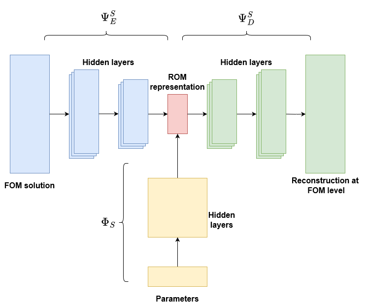
Figure 1: Basic DL-ROM architecture: encoder $\Psi_{E}^{S}$ and decoder $\Psi_{D}^{S}$ are trained to minimize reconstruction error between full order model solution and its reconstruction, After training, encodings of solutions are calculated with encoder $\Psi_{E}^{S}$ and Multilayer perceptron (MLP) $\Phi_{S}$ is trained to map parameters to encoding. To obtain a solution for new parameters $\bm{\lambda}$, parameters are passed through $\Phi_{S}$ and then through the decoder $\Psi_{D}^{S}$.

Notice that getting solutions from this kind of reduced-order model doesn’t require solving any additional equations and can be efficiently done for multiple parameters at the same time, suing GPU parallel computing. In this work, Convolutional Neural Networks (CNN) [32] were used for the encoder and decoder and all domains involved were rectangular.

2.4 Deep Learning Proper Orthogonal Decomposition ROM

Deep Learning Proper Orthogonal Decomposition ROM (POD-DL-ROM) was introduced in [33]. The procedure goes as follows. Solutions $\bm{u}_{i},i=1,\ldots N$ are reshaped into vectors of length $N_{h}$ and assembled into a matrix $\mathbf{A}$ with $N_{h}$ rows and $N$ columns. Columns of matrix $\mathbf{A}$ are $\bm{a}_{i},i=1,2,\ldots N$. The essence of the POD method is to get orthonormal vectors $\bm{\Phi_{i}},i=1,2,\ldots k$, $k\ll N$ vectors that maximize:

$$\frac{1}{N}\sum_{i=1,\ldots N,j=1,\ldots k}|\langle\bm{a}_{i},\bm{\Phi}_{j}\ \rangle|^{2}$$

So, the following approximation hold:

$$\bm{u}\approx\mathbf{V}_{k}\bm{u}_{k}$$

Matrix $\mathbf{V}_{k}$ is usually found using SVD decomposition or randomized SVD (rSVD) [34]. So, the solution $u$ can be approximated with POD basis and represented as $k$-dimensional vector $[\langle\bm{u},\bm{\Phi}_{1}\rangle,\ldots\langle\bm{u},\bm{\Phi}_{k}\rangle]$. Then, similar to the black-box DL-ROM, the model consists of three networks: encoder $\Psi_{E}$, decoder $\Psi_{D}$, and parameter-encoding network $\Phi$. The difference is that the encoder and decoder are trained on POD coefficients, thus reducing the dimension of the problem. For this model to work on multiple domains, POD coefficients at the reference domain and mapping between domain and reference domain are needed.

2.5 Graph convolutional autoencoder approach for DL-ROMs

Following DL-ROM framework, in [35] Graph convolutional autoencoders (GNNs) [36], [37], [38], [39] are used for dimension reduction. Using the proposed autoencoder technique, one can obtain ROM for non-rectangle domains using the GNN autoencoder. In the proposed approach, graph pooling and a fully-connected layer work only when all domains have the same number of nodes and domain parametrization is known as well. In applications, especially in biomedicine, both constraints may not hold.

3 Our method

In this work, we develop an efficient Reduced Order Model (ROM) that operates effectively across different domains, based on a Deep Learning Reduced Order Model (DL-ROM) approach. We refer to our method as Deep Learning domain aware ROM (DL-DA ROM). To achieve this, meaningful parametrization of domains is essential. Domains can be described parametrically, may evolve as part of the system (e.g., moving domains), or can be obtained from measurements.

Since the ROM for given parameters has to predict the domain and values of solutions on that domain, we separate those two tasks. In this work, we assume that the solution is at least continuous and can be interpolated onto rectangular mesh without significant loss of accuracy, see Figure 2. By interpolating in this manner, Convolutional neural networks (CNNs) can be utilized to construct an autoencoder for solutions. This approach is particularly beneficial in scenarios where the domain is derived from measurements and meshing is prohibitively expensive.

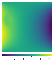
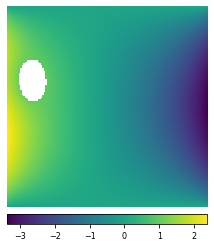
Figure 2: Sample interpolated onto equidistant rectangular grid (on the left). Sample (on the right).

When domains are parametrically described, it is not necessary to assume that each domain has the same number of parameters; they may have varying numbers of subdomains or holes. Our approach assumes that each domain characteristic function can be interpolated onto a rectangular grid, see Figure 3.

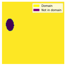
Figure 3: Mesh representation of the domain (left), an image of domain characteristic function (right).

The domain of the problem can be derived either from measurements or parameters. In our proposed method, its characteristic function is described as a bitmap image, with pixels assigned a value of one or zero depending on whether the pixel is inside or outside the domain. A convolutional autoencoder is trained using binary cross-entropy loss [40] to classify each pixel as part of the domain or not which is given by

$$l(x,y)=\frac{1}{nm}\sum_{i=1}^{n}\sum_{j=1}^{m}-y_{ij}\log(x_{ij})-(1-y_{ij})\log(1-x_{ij}),$$

where $\bm{y}$ is target bitmap image with $n$ rows and $m$ columns and $\bm{x}$ is network output image, whose pixels values $x_{ij}$ denote probability that pixel $x_{ij}$ is equal to one. The encoded domains are then used as the parametrization of the domain. The domain autoencoder is inspired by semantic segmentation encoder-decoder models in computer vision [41], [42], with two classes indicating whether a pixel is inside or outside the domain. This approach can be extended to problems with multiple domains, such as fluid-structure interaction problems, providing simultaneous geometric parametrization for the entire system. If domains can be generated synthetically, it is possible to use more samples for the domain autoencoder than for the solution autoencoder.

Domain autoencoder is shown in Figure 4.

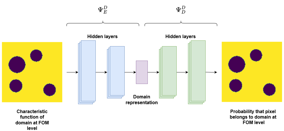
Figure 4: Domain Autoencoder used for domain parametrization. Input to the convolutional neural network is a characteristic function represented as a bitmap image. The output of the autoencoder is a rectangular grid with the probability that a given pixel belongs to the domain. The encoder output is used as domain parametrization.

If the domain is either known from measurements or is parametrized, the encoding of the domain can be used as additional parameters in the network $\Phi$. The model is shown in Figure 5 and all important terms in this work are given in table 1.

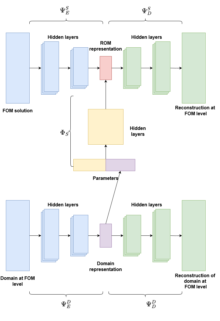
[sca]

Figure 5: Deep ROM for parametric domains: In addition to vanilla Deep ROM, we introduce domain autoencoder, which extracts parameters for the domain. These encodings are then used as additional parameters in Deep ROM.

label meaning $\Omega(\bm{\lambda})$ domain of the problem, in our work, is dependent on parameters $\Psi_{E}^{S}$ solution encoder $\Psi_{D}^{S}$ solution decoder $\Phi_{S}$ neural network that maps parameters into solution encoding $\Psi_{E}^{D}$ domain encoder $\Psi_{D}^{D}$ domain decoder

Table 1: Notation used in this work.

Constructing the ROM, also known as the offline phase, involves gathering the data, either with numerical simulation, measurements, or possibly a combination of both. Domain and solution autoencoders are trained to obtain meaningful low-dimensional encodings. Before training the solution autoencoder training solution data is standardized by applying the following transformation:

$$\bm{u}_{i}=\frac{\bm{u}_{i}-\mu_{s}}{\sigma_{s}},1,\ldots N$$

where $N$ is a number of samples in the training dataset, $\mu_{s}$ and $\sigma_{s}$ are mean and standard deviation of the training dataset After training the solution and domain autoencoders, domain encoding, and other equation parameters are concatenated. Training parameters are standardized by applying the following transformation:

$$\lambda_{ij}=\frac{\lambda{ij}-\mu_{pj}}{\sigma_{pj}},i=1,\ldots N,j=1\ldots k$$

where $k$ is dimension of parameter vector, $N$ number of samples and $\mu_{pj},\sigma_{pj}$ are mean and standard deviation of each parameter separately. Afterward, the network $\Phi_{S}$ is trained to predict solution encodings from parameters.

The procedure is summarized in Algorithm 1. After all data collection and training are completed, solutions for unseen parameters are calculated in the online phase, as detailed in Algorithm 2. For new values of equation parameters and domain, this involves passing the domain through the domain encoder $\Psi_{E}^{D}$ concatenating the resulting encoding with the equation parameters, passing them through the MLP $\Phi_{S}$ and finally through the solution decoder $\Psi_{D}^{S}$ to obtain prediction $\hat{u}$. The final ROM solution is then given by:

$$\bm{u}=\sigma_{s}\bm{u}+\mu_{s}$$

Algorithm 1 Offline phase

Parameter-solution-characteristic function triplets $(\bm{\lambda}_{i},\bm{u}_{i},\bm{c}_{i}),i=1,\ldots N$, hyperparameters for training of networks $\Psi_{E}^{S},\Psi_{D}^{S}$, domain autoencoder $\Psi_{E}^{D},\Psi_{D}^{D}$, and parameter-encoding network $\Phi_{S}$

Trained networks

Standardize solution data

Train solution encoder $\Psi_{E}^{S}$ and decoder $\Psi_{D}^{S}$ to minimize reconstruction loss $\frac{1}{N}\sum_{i=1}^{N}\|\bm{u}_{i}-\Psi_{D}^{S}(\Psi_{E}^{S}(\bm{u}_{i}))\|^{2}$

Evaluate trained $\Psi_{E}^{S}$ on $\bm{u}_{i},i=1,\ldots N$ and get encodings $\bm{e}_{i}=\Psi_{E}^{S}(\bm{u}_{i}),i=1,\ldots N$

Train domain encoder $\Psi_{E}^{D}$ and decoder $\Psi_{D}^{D}$ to minimize binary cross-entropy loss

Evaluate trained $\Psi_{E}^{D}$ and get domain parameters $\bm{d}_{i}=\Psi_{E}^{D}(\bm{c}_{i}),i=1,\ldots N$

Concatenate domain and equation parameters $\bm{d}_{i}$ and $\bm{\lambda}_{i}$ into new parameters $\bm{f}_{i},i=1,\ldots N$

Standardize new parameters $\bm{f}_{i},i=1,\ldots N$

Train $\Phi_{S}$ to minimize reconstruction loss $\frac{1}{N}\sum_{i=1}^{N}\|\Phi_{S}(\bm{f}_{i})-\bm{e}_{i}\|^{2}$

Save all trained networks

Save mean $\mu_{s}$ and standard deviation $\sigma_{s}$ of training dataset and mean $\mu_{p}$ and standard deviation $\sigma_{p}$ of training feature dataset

Algorithm 2 Online phase

: Neural networks $\Psi_{D}^{S},\Psi_{E}^{D}$, and $\Phi_{S}$, values of parameters and/or domains for which we want to evaluate solution $(\bm{\lambda}_{i},\bm{c}_{i}),i=1,\ldots M$, mean and standard deviation of training parameters $\bm{f}_{i}$ $\mu_{p},\sigma_{p}$, mean and standard deviation of solutions $\mu_{s},\sigma_{s}$

Solutions for given parameters and domains $\bm{u}_{i},i=1,\ldots M$

Compute domain parameters $\bm{d}_{i}=\Psi_{E}^{D}(\bm{c}_{i})$

Concatenate $f_{i}=(\bm{\lambda}_{i},\bm{d}_{i}),i=1,\ldots M$

Standardize $\bm{f}_{i}$ based on training mean and standard deviation

Calculate ROM prediction $\bm{\hat{u}}=\Psi_{D}^{S}(\Phi_{S}(\bm{f}_{i}))$

Return solution $\sigma_{s}\bm{\hat{u}}+\mu_{s}$

Experiments and Results

Through this section, we will use relative error to evaluate our approach. The relative error $\epsilon$ for sample $(\bm{\lambda},\bm{u}_{h},\bm{d}_{h})$ is:

$$\epsilon(\bm{u}_{h},\hat{\bm{u}_{h}})=\frac{\sqrt{\sum_{i,j}(u^{i,j}_{h}d^{i,j}_{h}-\hat{u}^{i,j}_{h}d^{i,j}_{h})^{2}}}{\sqrt{\sum_{i,j}(u^{i,j}_{h})^{2}d^{i,j}_{h}}},$$

where $\bm{\lambda}$ is the parameter vector, $\bm{u}_{h}$ solution discretized on a mesh with $n\times m$ points, $\bm{\hat{u_{h}}}$ is DL-ROM prediction and $\bm{d}_{h}$ is an approximation of characteristic functions of the domains on that same mesh.
Relative error at i-th row and j-th column is:

$$\epsilon_{i,j}(u_{k},\hat{u}_{h})=\frac{u_{h}^{i,j}d_{h}^{i,j}-\hat{u}^{i,j}_{h}d^{i,j}_{h}}{\sqrt{\sum_{k,l}(u^{k,l}_{h})^{2}d^{k,l}_{h}}},$$

where $u^{i,j}_{h},\hat{u}^{i,j}_{h},d^{i,j}_{h}$ are discretized solutions, model approximation of the solution, and characteristic function value in i-th row and j-th column.
We use FEM implementation in FreeFEM [43] to obtain solutions and Pytorch [44] for defining and training neural networks. All solutions are projected on a rectangular equidistant mesh, in order to use CNN. In all examples, Leaky ReLU is used as an activation function after convolution. We use batch normalization [45] after each layer, except for the last layers of the encoder and decoder. In all examples, the number of channels per layer in the decoder mirrors the encoder architecture. Upsampling operations are used only in some layers, such that the resolution of outputs in the decoder layers mirrors the resolution of outputs in the encoder layers. For all networks, Adam optimizer [46] with One Cycle Policy scheduling [47] is used that adjusts the learning rate at each training step, with a maximum of 1e-3 for the encoder-decoder network.
All training, test, and validation sets used have $1000$ samples. The batch size for the autoencoder is $50$. Autoencoder network hyperparameters were chosen by trial and error with respect to autoencoder reconstruction, where we searched on latent dimensions $15,20,30$ and the number of channels for each encoder layer (the decoder mirrors the encoder). Tried hyperparameters are shown in Table 2. Autoencoders with more channels per layer had better training and test accuracy, so we picked the best two for further analysis.

Latent dimension	$[15,20,30]$
Nbr. of kernels in encoder	$[4,4,8,8,16,16,16]$, $[4,8,16,32,32,64,64]$ , $[8,16,16,32,64,64,64]$
Learning rate	1e-3
Batch size	50
Kernel size	5

Table 2: Autoencoder grid search hyperparameters. We trained 9 models with varying channel sizes and latent dimension sizes. The number of channels in decoder layers mirrors the encoder number of channels per layer. We have chosen two autoencoders with the smallest reconstruction errors on the test set, both with $8,16,16,32,64,64,64,64$ channels in encoders and dimensions $20$ and $30$ for further analysis.

We have not encountered any overfitting problems by increasing autoencoder capacity. However, neural network $\Phi_{S}$ easily overfits. Since $\Phi_{S}$ is usually small compared to autoencoder and trains fast, we employed grid search to choose the best hyperparameters for $\Phi_{S}$. Hyperparameters are shown in Table 3. The grid search was done for two ROM representations, obtained from solution autoencoders with $8,16,16,32,64,64,64$ channels per layer and latent dimensions equal to $15$ and $30$, respectively. Domain features are obtained from autoencoders trained on $50000$ domains with $32,32,64,64,64,64,64,64$ channels per layer in each layer and strides $1,1,2,2,2,1,1,1$ per layer respectively. For each model, the One Cycle Policy scheduler with Adam optimizer was used. We have trained two different domain autoencoders, one with latent dimension $15$ and one with latent dimension $30$. We choose the best hyperparameters with respect to the mean-squared error between the prediction of $\Phi_{S}$ and ROM representation.

Hyperparameter	Values
Training set size	1000
Number of epochs	1500
Number of layers	1,2,3,4
Neurons per layer	64, 128, 256, 512, 1204, 2048
Dropout rate	0, 0.025, 0.05, 0.1, 0.2
Maximum learning rate	1e-5, 3.16e-5, 1e-4, 3.16e-4, 1e-3, 3.16e-3, 1e-2
Batch size	$8,16,32,64,128$

Table 3: Hyperparameters grid search for $\Phi$ is performed, which results in total $4200$ models.

3.1 Advection-diffusion on different domains

Advection-diffusion equation on parametric domains:

$$\begin{cases}-\Delta u+0.1\mathbf{c}\cdot\nabla u=1&\text{on $\langle 0,1\rangle^{2}$ without elipse}\\ u=1&\text{ on edge of ellipse}\\ u=0&\text{for $y=0$ and $y=1$}\\ \frac{\partial u}{\partial\nu}=\beta&\text{ for $x=0$}\\ \frac{\partial u}{\partial\nu}=-\beta&\text{ for $x=1$}\end{cases}$$ (4)

Parameters are:

• transport angle $\phi\in[0,2\pi]$ which determines vector $\mathbf{c}=(cos(\phi),sin(\phi))$

• center of ellipse $(x_{0},y_{0})\in[0.1,0.9]^{2}$

• angle of major axis of ellipse and x-axis $\alpha\in[0,\pi]$

• $\beta\in[1,10]$

• half-axes for ellipse are then taken randomly from interval depending on the center and angle of the ellipse

In total, there are $7$ parameters.

In this example, we know exact geometric parametrization, so we can obtain DL-ROM performance with calculated and exact parametrization and directly compare those two. For each domain parametrization, we have trained a fully-connected neural network $\Phi_{S}$ with hyperparameters determined by grid search.

Comparison of vanilla DL-ROM and our approach is shown in Table 4. We compare DL-ROM performance when exact ellipse parameters are used with domain parametrization calculated with the autoencoder. In all cases, models with calculated ellipse parameters perform better on the test set than models with exact ellipse parameters. In fact, we report that more than $1300$ models out of $4200$ trained in grid search, performed better on parameters of domain obtained autoencoder than the best model trained on exact domain parameters, for each combination. In this case, it can be seen that vanilla DL-ROM is more sensitive to ROM dimension, than our approach. Results are shown on Figure 6.

test error, ROM encoding dimension 15, domain encoding dimension 20 test error, ROM encoding dimension 15, domain encoding dimension 30 test error, ROM encoding dimension 30, domain encoding dimension 20 test error, ROM encoding dimension 30, domain encoding dimension 30 exact ellipse parameters only 0.0554552 0.0554552 0.0605261 0.0605261 exact and calculated elipse parameters 0.0454250 0.0425800 0.0458577 0.0438216 calculated elipse parameters 0.0465742 0.0452926 0.0451946 0.0449190

Table 4: Comparison of DL-ROM and DL-DA ROM performance: Difference of performance on relative test errors depending on ROM encoding dimension and domain encoding dimension. We differentiate between cases where geometric parameters are exactly known (1st row), when we add domain-encoded features to exact geometric features (2nd row), and when we use only geometric parameters obtained by autoencoder (3rd row). We can see that using autoencoder domain parametrization is beneficial for model performance. We report on the best model for each ROM encoding dimension and domain encoding dimension. Models trained on calculated domain parameters perform better than models trained using only exact domain parameters.

Figure 6: Top row: Exact solution, left, network prediction for a model trained on exact domain parameters (center), network prediction for a model trained on approximated domain parameters. Bottom row: relative error for a model trained on exact domain parameters (left), relative error for a model trained on approximated domain parameters (middle), relative error for a model trained on both exact and calculated domain parameters (right). Results are shown for ellipse with center $(0.76,0.38)$, half-axes $a=0.14,b=0.11$ and angle $\alpha=1.51$, $\beta=6.92$, $\mu=0.29$. All models were trained on $1000$ samples.

3.2 Domains with varying number of parameters

We experiment again on the advection-diffusion equation on parametric domains. In this case, domains can depend on a different number of parameters. Such a domain may be difficult to parametrize by classical techniques. We are investigating domains that are squares with $1$ to $4$ circular holes. Equations are:

$$\begin{cases}-\Delta u+0.1\mathbf{c}\cdot\nabla u=1&\text{on $\langle 0,1\rangle^{2}$ whitout circles}\\ u=2&\text{ on edge of circles}\\ u=0&\text{ for $y=0$ and $y=1$}\\ \frac{\partial u}{\partial\nu}=\beta&\text{ for $x=0$}\\ \frac{\partial u}{\partial\nu}=-\beta&\text{ for $x=1$}\end{cases}$$ (5)

Parameters are:

• transport angle $\phi\in[0,2\pi]$ which determines vector $\mathbf{c}=(cos(\phi),sin(\phi))$

• $m\in[1,4]$ number of circular holes

• centers of holes $(x_{i},y_{i})$, $i=1,\ldots m$.

• circles radii $r_{i}$, $i=1,\ldots m$.

• $\beta\in[1,10]$

To generate domains, first, we randomly choose the number of circles $m$. Then we randomly choose the centers of circles so the distance between the centers and the square boundary is at least $0.1$. Finally, radii are chosen randomly so that the distance between all circles is at least $0.1$ and $r\in[0.05,0.2]$. This procedure ensures that circles do not overlap and that all circles are of reasonable size. We have chosen the same encoder-decoder architectures as in the previous example and after training solution autoencoders, a grid search was performed to obtain $\Phi_{S}$ hyperparameters. Results are shown in Table 5 and Figure 7. A larger ROM dimension mostly does not affect DL-ROM performance, while a smaller domain parametrization encoding dimension is beneficial in this case.

test error, ROM encoding dimension 15, domain encoding dimension 20 test error, ROM encoding dimension 15, domain encoding dimension 30 test error, ROM encoding dimension 30, domain encoding dimension 20 test error, ROM encoding dimension 30, domain encoding dimension 30 calculated domain parameters 0.0239904 0.0264217 0.0209590 0.0267886

Table 5: Difference of performance on relative test errors depending on ROM encoding dimension and domain encoding dimension. In this case, domains have varying numbers of parameters. We use only geometric parameters obtained by the autoencoder. We report on the best model for each ROM encoding dimension and domain encoding dimension.

Figure 7: Exact solutions (left), model prediction (middle), relative error (right) for model trained on $1000$ random samples for parameters $\beta=0.977$, $\mu=0.842$, with centers $(0.23,0.73),(0.57,0.22),(0.25,0.37),(0.79,0.79)$ and radii $0.11,0.10,0.14,0.10$ respectively.

Furthermore, we test how sensitive DL-DA ROM DL-ROM is on small perturbations of the circle boundary. The sensitivity of this model is especially important if we train on synthetically generated data and test only on possibly imprecisely measured domains and parameters. Instead of testing the trained model on a domain with circular holes, we test the model on predicting the correct solution when the domain is a unit square without ellipses. The idea is that these ellipses model slightly deformed circles. The correct solution is again generated using the finite element method. We tested on solutions with parameters $\beta=1.19617,\theta=1.71657$ with $4$ holes, with centers $(0.66555,0.35233),(0.56892,0.71108),(0.25424,0.21219),(0.22812,0.58991)$ and radii of non-deformed circles $0.11191,0.12318,0.10707,0.10653$ respectively. A comparison between FEM and our DL-ROM is shown in Figure 8. We tested how sensitive our model is to perturbations of the boundary. In these cases, instead of circular holes, we have elliptic holes. The relative error for increasing deformation is given in Table 6.

Ratio between small and large half-axis two half-axes in %	$\epsilon$
1	0.0101
0.95	0.0120
0.9	0.0142
0.8	0.0166

Table 6: Relative errors for the same $\beta$, $\theta$ and ellipse centers as in 8 ($\beta=1.19617$, $\theta=1.71657$). Ellipses have centers $(0.66555,0.35233),(0.56892,0.71108),(0.25424,0.21219),(0.22812,0.58991)$, radii of non-deformed circles $0.11191,0.12318,0.10707,0.10653$ respectively and varying rations between small and large half-axis. We can see an increase in relative error with higher deformation of the domain boundary, but the increase is not rapid.

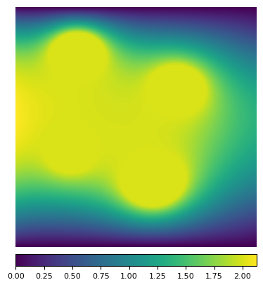
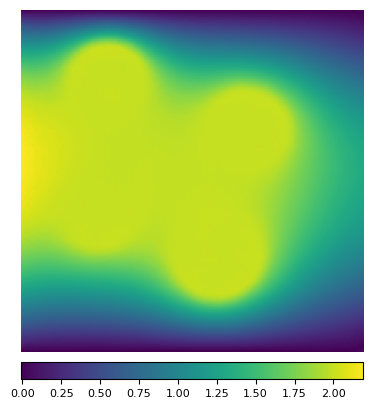
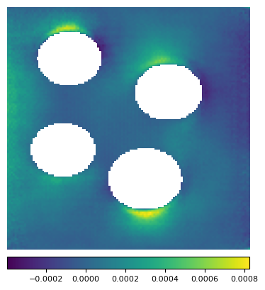
Figure 8: Exact solutions (left) not multiplied by characteristic function, model prediction (middle) not multiplied by characteristic function, relative error (right) multiplied by characteristic function for slightly deformed circles with parameters $\beta=1.19617$, $\theta=1.71657$. Ellipses have centers, $(0.66555,0.35233),(0.56892,0.71108),(0.25424,0.21219)$ and radii of non-deformed circles $0.11191,0.12318,0.10707,0.10653$ respectively. Small half-axes are $20\%$ smaller than large half-axes for each ellipse. Even though the model was not trained on elliptic holes, we can see a small relative error further from the boundary. The error is the largest at the boundary since the solution autoencoder did not capture ellipses in the original training dataset. This demonstrates that the model can work with small perturbations of the boundary.

Conclusion

In this work, we present the extension of DL-ROM to various 2D domains. This approach can be extended to 3D problems. Our algorithm can be used in problems where domains come from measurements. However, this comes at the expense of the main disadvantage of this approach, which is the first step of interpolating into a rectangular domain. In some problems, such as 3D thin pipes with torsion, rectangular data can be much larger than the actual number of nodes required to describe the pipe, which can be a computational bottleneck. In future work, we plan to mitigate this issue as well. We demonstrated that meaningful geometrical parametrization can be obtained using neural networks, which may be useful in other reduced-order model techniques as well.

References

- [1] Patrick LeGresley and Juan Alonso. Airfoil design optimization using reduced order models based on proper orthogonal decomposition. In Fluids 2000 conference and exhibit, page 2545, 2000.
- [2] Claudia Maria Colciago, Simone Deparis, and Alfio Quarteroni. Comparisons between reduced order models and full 3d models for fluid–structure interaction problems in haemodynamics. Journal of Computational and Applied Mathematics, 265:120–138, 2014.
- [3] Daniella E Raveh. Reduced-order models for nonlinear unsteady aerodynamics. AIAA journal, 39(8):1417–1429, 2001.
- [4] José V Aguado, Antonio Huerta, Francisco Chinesta, and Elías Cueto. Real-time monitoring of thermal processes by reduced-order modeling. International Journal for Numerical Methods in Engineering, 102(5):991–1017, 2015.
- [5] Alfio Quarteroni, Andrea Manzoni, and Federico Negri. Reduced basis methods for partial differential equations: an introduction, volume 92. Springer, 2015.
- [6] Alfio Quarteroni and Alberto Valli. Numerical Approximation of Partial Different Equations, volume 23. Springer Berlin, Heidelberg, 01 1994.
- [7] Qian Wang, Jan S Hesthaven, and Deep Ray. Non-intrusive reduced order modeling of unsteady flows using artificial neural networks with application to a combustion problem. Journal of computational physics, 384:289–307, 2019.
- [8] Stefania Fresca, Luca Dede’, and Andrea Manzoni. A comprehensive deep learning-based approach to reduced order modeling of nonlinear time-dependent parametrized pdes. Journal of Scientific Computing, 87:1–36, 2021.
- [9] Kookjin Lee and Kevin T Carlberg. Model reduction of dynamical systems on nonlinear manifolds using deep convolutional autoencoders. Journal of Computational Physics, 404:108973, 2020.
- [10] Peter Benner, Wil Schilders, Stefano Grivet-Talocia, Alfio Quarteroni, Gianluigi Rozza, and Luís Miguel Silveira. Model Order Reduction: Volume 2: Snapshot-Based Methods and Algorithms. De Gruyter, 2020.
- [11] George Cybenko. Approximation by superpositions of a sigmoidal function. Mathematics of control, signals and systems, 2(4):303–314, 1989.
- [12] Kurt Hornik, Maxwell Stinchcombe, and Halbert White. Multilayer feedforward networks are universal approximators. Neural networks, 2(5):359–366, 1989.
- [13] Ingrid Daubechies, Ronald DeVore, Simon Foucart, Boris Hanin, and Guergana Petrova. Nonlinear approximation and (deep) relu networks. Constructive Approximation, 55(1):127–172, 2022.
- [14] Alfio Quarteroni and Alberto Valli. Numerical approximation of partial differential equations, volume 23. Springer Science & Business Media, 2008.
- [15] Anindya Chatterjee. An introduction to the proper orthogonal decomposition. Current science, pages 808–817, 2000.
- [16] Gene H Golub and Christian Reinsch. Singular value decomposition and least squares solutions. In Handbook for Automatic Computation: Volume II: Linear Algebra, pages 134–151. Springer, 1971.
- [17] Saifon Chaturantabut and Danny C Sorensen. Nonlinear model reduction via discrete empirical interpolation. SIAM Journal on Scientific Computing, 32(5):2737–2764, 2010.
- [18] Thomas W Sederberg and Scott R Parry. Free-form deformation of solid geometric models. In Proceedings of the 13th annual conference on Computer graphics and interactive techniques, pages 151–160, 1986.
- [19] Filippo Salmoiraghi, Francesco Ballarin, Giovanni Corsi, Andrea Mola, Marco Tezzele, Gianluigi Rozza, et al. Advances in geometrical parametrization and reduced order models and methods for computational fluid dynamics problems in applied sciences and engineering: overview and perspectives. In Proceedings of the ECCOMAS Congress 2016, 7th European Conference on Computational Methods in Applied Sciences and Engineering, Crete Island, Greece, June 5-10, 2016, volume 1, pages 1013–1031. Institute of Structural Analysis and Antiseismic Research School of Civil …, 2016.
- [20] Gianluigi Rozza, Haris Malik, Nicola Demo, Marco Tezzele, Michele Girfoglio, Giovanni Stabile, and Andrea Mola. Advances in reduced order methods for parametric industrial problems in computational fluid dynamics. arXiv preprint arXiv:1811.08319, 2018.
- [21] Andrea Manzoni, Alfio Quarteroni, and Gianluigi Rozza. Model reduction techniques for fast blood flow simulation in parametrized geometries. International journal for numerical methods in biomedical engineering, 28(6-7):604–625, 2012.
- [22] AM Morris, CB Allen, and TCS Rendall. Cfd-based optimization of aerofoils using radial basis functions for domain element parameterization and mesh deformation. International journal for numerical methods in fluids, 58(8):827–860, 2008.
- [23] Donald Shepard. A two-dimensional interpolation function for irregularly-spaced data. In Proceedings of the 1968 23rd ACM national conference, pages 517–524, 1968.
- [24] Jeroen Witteveen and Hester Bijl. Explicit mesh deformation using inverse distance weighting interpolation. In 19th AIAA Computational Fluid Dynamics, page 3996. 2009.
- [25] Davide Forti and Gianluigi Rozza. Efficient geometrical parametrisation techniques of interfaces for reduced-order modelling: application to fluid–structure interaction coupling problems. International Journal of Computational Fluid Dynamics, 28(3-4):158–169, 2014.
- [26] Dongwei Ye, Valeria Krzhizhanovskaya, and Alfons G Hoekstra. Data-driven reduced-order modelling for blood flow simulations with geometry-informed snapshots. Journal of Computational Physics, 497:112639, 2024.
- [27] Wenqian Chen, Qian Wang, Jan S. Hesthaven, and Chuhua Zhang. Physics-informed machine learning for reduced-order modeling of nonlinear problems. Journal of Computational Physics, 446:110666, 2021.
- [28] M. Raissi, P. Perdikaris, and G.E. Karniadakis. Physics-informed neural networks: A deep learning framework for solving forward and inverse problems involving nonlinear partial differential equations. Journal of Computational Physics, 378:686–707, 2019.
- [29] Nicola Franco, Andrea Manzoni, and Paolo Zunino. A deep learning approach to reduced order modelling of parameter dependent partial differential equations. Mathematics of Computation, 92(340):483–524, nov 2022.
- [30] Geoffrey E Hinton and Ruslan R Salakhutdinov. Reducing the dimensionality of data with neural networks. science, 313(5786):504–507, 2006.
- [31] Simon Haykin. Neural networks: a comprehensive foundation. Prentice Hall PTR, 1998.
- [32] Yann LeCun, Bernhard Boser, John Denker, Donnie Henderson, R. Howard, Wayne Hubbard, and Lawrence Jackel. Handwritten digit recognition with a back-propagation network. In D. Touretzky, editor, Advances in Neural Information Processing Systems, volume 2. Morgan-Kaufmann, 1989.
- [33] Stefania Fresca and Andrea Manzoni. POD-DL-ROM: Enhancing deep learning-based reduced order models for nonlinear parametrized PDEs by proper orthogonal decomposition. Computer Methods in Applied Mechanics and Engineering, 388:114181, jan 2022.
- [34] N. Halko, P. G. Martinsson, and J. A. Tropp. Finding structure with randomness: Probabilistic algorithms for constructing approximate matrix decompositions. SIAM Review, 53(2):217–288, 2011.
- [35] Federico Pichi, Beatriz Moya, and Jan S. Hesthaven. A graph convolutional autoencoder approach to model order reduction for parametrized pdes, 2023.
- [36] Jie Zhou, Ganqu Cui, Shengding Hu, Zhengyan Zhang, Cheng Yang, Zhiyuan Liu, Lifeng Wang, Changcheng Li, and Maosong Sun. Graph neural networks: A review of methods and applications. AI open, 1:57–81, 2020.
- [37] Federico Monti, Davide Boscaini, Jonathan Masci, Emanuele Rodola, Jan Svoboda, and Michael M Bronstein. Geometric deep learning on graphs and manifolds using mixture model cnns. In Proceedings of the IEEE conference on computer vision and pattern recognition, pages 5115–5124, 2017.
- [38] Jiwoong Park, Minsik Lee, Hyung Jin Chang, Kyuewang Lee, and Jin Young Choi. Symmetric graph convolutional autoencoder for unsupervised graph representation learning. In Proceedings of the IEEE/CVF international conference on computer vision, pages 6519–6528, 2019.
- [39] Yi Zhou, Chenglei Wu, Zimo Li, Chen Cao, Yuting Ye, Jason Saragih, Hao Li, and Yaser Sheikh. Fully convolutional mesh autoencoder using efficient spatially varying kernels. Advances in neural information processing systems, 33:9251–9262, 2020.
- [40] Zhilu Zhang and Mert Sabuncu. Generalized cross entropy loss for training deep neural networks with noisy labels. Advances in neural information processing systems, 31, 2018.
- [41] Vijay Badrinarayanan, Alex Kendall, and Roberto Cipolla. Segnet: A deep convolutional encoder-decoder architecture for image segmentation. IEEE transactions on pattern analysis and machine intelligence, 39(12):2481–2495, 2017.
- [42] Hyeonwoo Noh, Seunghoon Hong, and Bohyung Han. Learning deconvolution network for semantic segmentation. In Proceedings of the IEEE international conference on computer vision, pages 1520–1528, 2015.
- [43] F. Hecht. New development in freefem++. J. Numer. Math., 20(3-4):251–265, 2012.
- [44] Adam Paszke, Sam Gross, Francisco Massa, Adam Lerer, James Bradbury, Gregory Chanan, Trevor Killeen, Zeming Lin, Natalia Gimelshein, Luca Antiga, Alban Desmaison, Andreas Kopf, Edward Yang, Zachary DeVito, Martin Raison, Alykhan Tejani, Sasank Chilamkurthy, Benoit Steiner, Lu Fang, Junjie Bai, and Soumith Chintala. Pytorch: An imperative style, high-performance deep learning library. In Advances in Neural Information Processing Systems 32, pages 8024–8035. Curran Associates, Inc., 2019.
- [45] Sergey Ioffe and Christian Szegedy. Batch normalization: Accelerating deep network training by reducing internal covariate shift. In International conference on machine learning, pages 448–456. pmlr, 2015.
- [46] Diederik P Kingma and Jimmy Ba. Adam: A method for stochastic optimization. arXiv preprint arXiv:1412.6980, 2014.
- [47] Leslie N Smith and Nicholay Topin. Super-convergence: Very fast training of neural networks using large learning rates. In Artificial intelligence and machine learning for multi-domain operations applications, volume 11006, pages 369–386. SPIE, 2019.