Bayesian non-linear subspace shrinkage using horseshoe priors

Abstract

When modeling biological responses using Bayesian non-parametric regression, prior information may be available on the shape of the response in the form of non-linear function spaces that define the general shape of the response. To incorporate such information into the analysis, we develop a non-linear functional shrinkage (NLFS) approach that uniformly shrinks the non-parametric fitted function into a non-linear function space while allowing for fits outside of this space when the data suggest alternative shapes. This approach extends existing functional shrinkage approaches into linear subspaces to shrinkage into non-linear function spaces using a Taylor series expansion and corresponding updating of non-linear parameters. We demonstrate this general approach on the Hill model, a popular, biologically motivated model, and show that shrinkage into combined function spaces, i.e., where one has two or more non-linear functions a priori, is straightforward. We demonstrate this approach through synthetic and real data. Computational details on the underlying MCMC sampling are provided with data and analysis available in an online supplement.

1 Introduction

When modeling complex biological systems, mechanistic knowledge about the system under investigation is often available; however, including this information in a statistical model may be impossible due to the system’s complexity in relation to experimental and computational resources [Mesarovic et al., 2004]. Often, simplified models are used in lieu of the true mechanistic model [Šimon, 2005]. When using these simplified models, one expects them to describe the observed data correctly or be mildly misspecified, and in the case of misspecification, the model may still be helpful in describing the response.

When modeling biological systems, an example of this situation is the use of the Hill model. This model, which represents sigmoidal-shaped responses, is a simplification of the complex biochemical process based upon chemical kinetics [Hill, 1910] and is used to model a wide variety of biochemical processes [Goutelle et al., 2008]. Despite its widespread use, it may not always represent the observed response. Non-monotone deviations of the Hill’s functional form may be evident in the data. Additionally, other competing models may also be available, and the modeler might like to include this information to inform the fitting process, too. We develop a framework that allows one to define a subspace over one or more function spaces of interest for Bayesian non-parametric regression.

From the Bayesian perspective, there is a rich literature on approaches incorporating prior knowledge in non-parametric regression. Naively, one may center the non-parametric model on the specified parametric function. When the parametric data-generating mechanism’s mean is the known parametric model, ensuring that estimates do not contain artifactual deviations from that model is difficult, implying that shrinkage to the prior model will not be uniform. Further, using this method, there is no way to create a space based on multiple parametric functions. More sophisticated approaches use shape constraints induced through the prior distribution, which include monotonicity or limits to the number of extrema [Brezger and Steiner, 2008, Shively et al., 2009, Meyer, 2008, Shively et al., 2011, Meyer et al., 2011, Gunn and Dunson, 2005, Köllmann et al., 2014, Wheeler et al., 2017]. Though these approaches are often effective, they do not directly incorporate parametric modeling information on the shape of the model; they force the response to be in the constrained space by putting a prior mass of zero on all responses outside of that space.

Alternatively, one may merge mechanistic prior knowledge into a model is through ordinary differential equations (ODEs) within a Bayesian framework. Parametric Bayesian models include pharmacokinetic/pharmacodynamic modeling, discussed by Lunn et al. [2002], and Huang et al. [2006] present an HIV-modeling example using Bayesian hierarchical models with non-linear differential equations. More flexible non-parametric approaches use differential equations to inform stochastic processes with induced constraints [Golightly and Wilkinson, 2011, Titsias et al., 2012]. While Alvarez et al. [2013] and Wheeler et al. [2014] proposed a Gaussian Process (GP) approach that incorporates mechanistic knowledge defined by differential equations. More recently, Chen et al. [2022] incorporate mechanistic knowledge defined by linear or non-linear partial differential equations (PDE) into a GP framework by selecting PDE points, i.e. pseudo covariate points through which the assumed PDE information is incorporated. Like the shape-constrained approaches, these methods form a Basis expansion consistent with a subspace defined using mechanistic knowledge. Thus, these priors imply that an estimated function is within the given subspace, and they do not allow for deviations outside of this space.

We define a prior distribution over a non-linear subspace - such as the Hill model and power model - that does not require a fitted function to be within that subspace. When the non-linear subspace is correctly specified, shrinkage into it occurs; but, when the true model is outside of the subspace, the approach is unconstrained. We build upon the work of Shin et al. [2020] who introduced the functional horseshoe (fHS) prior for linear spaces. The fHS prior shrinks the non-parametric fit towards a pre-specified, linear subspace. This approach is different from well-known shrinkage approaches such as Ridge, Lasso or Horseshoe [Hoerl and Kennard, 1970, Tibshirani, 1996, Carvalho et al., 2010], which shrink model coefficients in a non-parametric regression towards the origin. The prior of Shin et al. [2020] has the appealing property that the posterior shrinks into the pre-specified subspace f it is consistent with the observed data or, alternatively, is left unconstrained otherwise. The shrinkage occurs at the minimax optimal rate.

In our extension, we use a Taylor expansion to locally linearize the response function, where the derivatives depend on parameters of the non-linear model. The extension allows functional shrinkage into a non-linear function space or adapts the function to be outside of the non-linear space. The relevant non-linear function space is specified a priori using one or more parametric models.

We present our shrinking approach in Section 2. Section 3 then illustrates the approach both for the case of shrinkage into a single function space - shown for the Hill model - and into a combined function space - shown for the Hill and the power models. We compare our method against other parametric and non-parametric approaches in a simulation study in Section 4. We apply our method to a real-world data example of total testosterone levels measured in 9943 males aged between 3 and 85 years in section 5. The computational back-bone of the approach is MCMC sampling combining Gibbs-, Metropolis-Hastings- and Slice-sampling [Brooks et al., 2011, Neal, 2003], detailed in the supplementary material.

2 Model

2.1 Spline Model

Consider the non-parametric regression problem

$$y_{i}=g(x_{i})+\varepsilon_{i},$$ (1)

with unknown mean function $g:\mathbb{R}\rightarrow\mathbb{R}.$ We observe $y=(y_{1},\dots,y_{n})^{\prime}$ corresponding to covariates $x=(x_{1},\dots,x_{n})^{\prime}$ and wish to estimate $g.$ Assuming $\varepsilon_{i}\overset{\text{iid}}{\sim}N(0,\sigma^{2}),$ it is common to approximate $g$ using a B-spline basis expansion [Carl, 2001], i.e.,

$$f(x_{i})=\sum_{m=1}^{k}\phi^{j}_{m}(x_{i})\beta_{m},$$ (2)

or $f(x)=\Phi\beta$. Here, the B-spline basis $\phi_{k}^{j}(x)$ are of order $j$ defined on $k^{*}$ internal knots, where $k=k^{*}+j,$ $\beta=(\beta_{1},\dots,\beta_{k})^{\top}$ denotes the vector of basis coefficients. We consider cubic splines and omit the superscript $j=3$. With a dense knot set, the spline approximation $f$ can be made to be arbitrarily close to any continuous $g,$ allowing one to estimate a large space of functions to arbitrary precision.

2.2 Bayesian Priors for a Non-linear Subspace

For many prior specifications, the expansion in (2) may not place high prior probability on biologically relevant responses. To define a biologically relevant model, we construct a prior distribution that places significant prior mass on the function space defined by the non-linear model, e.g., the space of Hill models, but does not put zero mass outside the function space.

To do this, assume knowledge about the shape of $g$ through a twice differentiable function $h_{\theta}:\mathbb{R}\rightarrow\mathbb{R}$. The function $h_{\theta}$ depends on parameter vector $\theta,$ and defines the function space $\Omega^{\Theta}_{0}=\{h_{\theta}|\theta\in\Theta\}$ for all realizations $\Theta\subseteq\mathbb{R}^{s}$. If the true mean function $g$ happens to be outside $\Omega^{\Theta}_{0}$, shrinkage towards $\Omega^{\Theta}_{0}$ is undesirable. Given a dense knot set, the spline $f$ can approximate $h_{\theta}$ for any $\epsilon-$ball. Consequently, the space of functions represented by the spline contains $\Omega^{\Theta}_{0}.$ We define a prior for (2) that places prior mass on $\Omega^{\Theta}_{0},$ but does not limit responses to be only in $\Omega^{\Theta}_{0}$.

To define this prior, we consider Shin et al. [2020], who defined a projection prior that shrinks into the linear column space defined by the matrix $\Phi_{0}\in\mathbb{R}^{n\times d}$ through

$$p(\beta|\sigma^{2},\tau^{2})\propto(\tau^{2})^{-(k-d_{0})/2}\exp\left(-\frac{1}{2\sigma^{2}\tau^{2}}\beta^{\top}\Phi^{\top}(I-P_{\Phi_{0}})\Phi\beta\right),$$ (3)

where $d_{0}=\text{rank}(\Phi_{0}),$ $\Phi_{0}$ is constructed as a linear space of known covariates, and $P_{\Phi_{0}}$ is the orthogonal projection matrix into the column space of $\Phi_{0}.$ The hyperparameter $,\tau,$ is given a generalized horseshoe (HS) prior with hyperparameters $a$ and $b$ (cf. Shin et al. [2020]). When $a=b=0.5$ the prior is a half-Cauchy distribution, and one arrives at the HS prior [Carvalho et al., 2010].

In (3), one constructs $P_{\Phi_{0}}$ using the linear column space of $\Phi_{0}.$ Given our space is non-linear, there is no direct analogue to $P_{\Phi_{0}}.$ As an approximation, we use a Taylor series approximation of $h_{\theta_{0}},$ $\theta_{0}\in\Theta.$ That is, we linearly approximate $\Omega^{\Theta}_{0}$ at any $\theta_{0}$ using a first-order Taylor expansion

$$h_{\theta}(x)\approx h_{\theta_{0}}(x)+\dot{\text{H}}_{\theta_{0}}(x)(\theta-\theta_{0})$$ (4)

where $\dot{\text{H}}_{\theta_{0}}(x)=\left.\frac{\partial h_{\theta}(x)}{\partial\theta}\right\rvert_{\theta=\theta_{0}}\in\mathbb{R}^{n\times s}$ is the Jacobian containing the partial derivatives of $h_{\theta}$ evaluated at $\theta_{0}$. The column space of $\dot{\text{H}}_{\theta}(x)$ approximates $h_{\theta}(x)$ [Seber and Wild, 2003][p. 130] and we use $\dot{\text{H}}_{\theta}(x)$ to construct $P_{\theta}=P_{\dot{\text{H}}_{\theta}}$. Thus, for any $\theta_{0}$, we project $f(x)$ onto the space locally approximating $h_{\theta_{0}}.$ When there are multiple function spaces to consider, the same approach applies; in this case, operator $P_{\dot{\text{H}}_{\theta}}$ defines the projection into a combined linear space, where $\dot{\text{H}}_{\theta}$ represents the Jacobian across all assumed functions.

We place the prior

$$p(\beta|\sigma^{2},\tau^{2},\theta)\propto(\tau^{2})^{-k/2}\exp\left(-\frac{1}{2\sigma^{2}\tau^{2}}\beta^{\top}\Phi^{\top}(I-P_{\theta})\Phi\beta\right)$$ (5)

over $\beta$ to shrink realizations of (2) into $\Omega^{\Theta}_{0}.$ In (5), $\theta$ is given an appropriate prior to complete the specification. This approach penalizes deviations of $\Phi\beta$ based upon the projection operator $(I-P_{\theta}).$ As we shrink back to a planar approximation given a specific $\theta_{0},$ we require appropriately specified priors for the non-linear parameters in $\Theta$. As $\beta$ is defined conditional on $\theta$ through the linear projection operator $P_{\theta},$ only priors for the non-linear parameters can be learned.

In this formulation, $(\tau^{2})^{-(k-d_{0})/2}$ in (3) becomes $(\tau^{2})^{-k/2}$ because we separately model the intercept (cf. Section 3.1). This change yields proper priors as due to the non-linearity, no linear basis of $\Phi$ is in $(I-P_{\theta})$ and $\Phi^{\top}(I-P_{\theta})\Phi$ has full rank.

3 Non-linear functional shrinkage for single or combined function spaces

3.1 Single function spaces

As an example of non-linear functional shrinkage using a single function, we consider the Hill model. This function is given by

$$h(x,\theta)=\theta_{1}+\theta_{2}\frac{x^{\theta_{4}}}{{\theta_{3}}^{\theta_{4}}+x^{\theta_{4}}},$$ (6)

where $\theta_{1}$ is the background response at $x=0$, $\theta_{2}$ is the maximal change in the response, $\theta_{3}$ is the dose where half of this change is reached and $\theta_{4}$ defines the steepness of the curve. The Jacobian, $\dot{\text{H}}_{\theta},$ is

$$\left.\frac{\partial h(x,\theta)}{\partial\theta}\right\rvert_{\theta=\theta_{0}}=\left.\begin{pmatrix}1&\frac{x^{\theta_{4}}}{x^{\theta_{4}}+{\theta_{3}}^{\theta_{4}}}&\theta_{2}\frac{-\theta_{4}}{\theta_{3}}s(x,\theta_{3},\theta_{4})&\theta_{2}\log(\theta_{3}/x)s(x,\theta_{3},\theta_{4})\end{pmatrix}\right\rvert_{\theta=\theta_{0}},$$ (7)

with $s(x,\theta_{3},\theta_{4})=((x{\theta_{3}}^{-1})^{\theta_{4}}+1)^{-1}((\theta_{3}x^{-1})^{\theta_{4}}+1)^{-1}$. The derivative matrix does not depend upon the linear parameters $\theta_{1}$, but it still depends on $\theta_{2}$. However, $P_{\theta}$ does not depend on $\theta_{1}$ and $\theta_{2}$ (cf. Lemma 1 in the appendix), which gives a direct example of why we do not place a prior over these linear quantities. Of the parameters in (7), parameter $\theta_{3}$ is of particular interest because it represents the value of $x$ that produces a response that is the average of the lower and upper asymptote. Values of the covariate below $\theta_{3}$ correspond to values of the response less than $50\%$ of the maximal response. Further, $\theta_{4}$ corresponds to the steepness of the response and speed of a chemical reaction in a biological substrate. As both quantities have direct interpretation, informative priors can be developed for these quantities accordingly, which in turn informs the subspace the model may shrink into.

To specify the hyperprior over $(\theta_{3},\theta_{4})$, we assume $x\in[0,1],$ and let $E[\theta_{3}]=0.5,$ the midpoint, and for $\theta_{4},$ we center it on $3$, letting the parameter vary within a range that we have often seen in bioassays. In our model, $\theta_{1}$ enters as the intercept, and $\theta_{2}$, the maximal response change, implicitly enters the model through the $\beta$ coefficients. Using the Hill model as a prior to define (5), we complete the prior specification as

$$(y|\beta,\sigma^{2},\theta_{1}) \sim N(\theta_{1}+\Phi\beta,\sigma^{2}I_{n})$$ (8)

$$\theta_{1}\sim N(0,20),\quad\theta_{3} \sim N_{+}(0.5,0.05)\quad\theta_{4}\sim LN(0.95,0.29)$$ (9)

$$\sigma^{2} \sim IG(0.001,0.001),$$ (10)

where $N_{+}(a,b)$ is a truncated normal distribution with mean $a$ and variance $b$ (before truncation), $LN(a,b)$ is a log-normal distribution with log-mean $a$ and log-variance $b,$ and $IG(a,b)$ is an inverse-gamma distribution with shape $a$ and scale $b$. Note that $\theta_{4}\sim LN(0.95,0.29)$ results in $E[\theta_{4}]=3$ and $V[\theta_{4}]=3$.

3.2 Combined function spaces

If one desires multiple functions to define in the function space because of uncertainty in the function space, one can add multiple functions. Here, assume there are $r\in\{1,\dots,R\}=\mathcal{R}$ function spaces $\Omega_{0}^{(r)}=\{h_{\theta}^{(r)}|\theta\in\Theta^{(r)}\}$ of interest; we omit the index $r$ on each $\theta$ for simplicity. For each $\Omega_{0}^{(r)},$ calculate the Jacobian, $\dot{\text{H}}_{\theta}^{(r)},$ i.e.,

$$\dot{\text{H}}_{\theta}^{(\mathcal{R})}=(\dot{\text{H}}_{\theta}^{(1)}\ldots\dot{\text{H}}_{\theta}^{(R)}),$$

and use this to construct $P_{\theta}.$ The Jacobian, $\dot{\text{H}}_{\theta}^{(\mathcal{R})},$ must be full rank without linear bases other than an intercept column for Equ. 5 to hold.

To illustrate the combined subspace shrinkage approach, we use the Hill and power models. The latter function defined as as $h_{\theta}(x)=\theta_{1}+\theta_{2}x^{\theta_{3}},$ which has only one non-linear parameter, $\theta_{3},$ that requires a prior specification. We use $\theta_{3}\sim N(0.5,0.25)$, to center on a concave shape. The partial derivatives of the power model are

$$\frac{\partial h(x,\theta)}{\partial\theta}=\left(1\quad x^{\theta_{3}}\quad\log(x)x^{\theta_{3}}\right)=\dot{\text{H}}_{\theta}^{(1)}.$$ (11)

Prior to combining $\dot{\text{H}}_{\theta}^{(1)}$ of the power model and $\dot{\text{H}}_{\theta}^{(2)}$ of the Hill model (Eq. 7), we remove the intercept from $\dot{\text{H}}_{\theta}^{(1)}$ to obtain a full rank. Shrinkage into the combined subspaces is equivalent to shrinkage into a single subspace.

4 Simulation Study

4.1 Setup

We perform a simulation study and evaluate the performance of the proposed approach against other fitting strategies. Full details of the simulation design are summarized by the ADEMP principle described in Morris et al. [2019] (Table S2). We generate data using three parametric cases: the Hill model, the power model, and a misspecified model (the Hill model with downturn). We look at exposure-response data as, for such data, chemical kinetics of exposure are often approximated by the Hill model, but the results generalize to other domains.

For each data set, we draw $x\in[0,1]$ uniformly for $n\in\{50,100,200,500\}$ observations, where $50$ is a realistic assay size and larger $n$ are chosen to study the large sample behavior. Mean zero normal noise with variance $\sigma^{2}=0.005$ and a larger noise $\sigma^{2}=0.05$ is added. These variances represent a 2-SD spread that is approximately $14\%$ and $45\%$ of the maximal response. In total, $24$ data generating scenarios are used, with $n_{\text{rep}}=1000$ simulations per scenario. For each dataset, we apply the following methods:

4.1.1 Modeling Approaches

Non-linear functional shrinkage (NLFS)

Non-linear functional shrinkage is performed with shrinkage into the Hill space (NLFS(Hill)), power space (NLFS(power)), or a combination (cf. Section 3.2) of both function spaces (NLFS(Hill+power)). Two variations for the shrinkage parameter $\tau^{2}$ are considered. One uses a half Cauchy prior ($a=b=0.5$) and is implemented according to Makalic and Schmidt [2015]; the other, implemented ourselves using slice sampling [Neal, 2003], uses a $\omega\sim\text{Beta}(a,b)$ prior where $a=0.5$ and $b=\exp(-k\log(n)/2)$ as proposed by Shin et al. [2020] and $k$ is the number of knots.

Parametric Model (Param.)

We investigate the performance fitting of the Oracle model using Bayesian parametric regression for the Hill model (Param.(Hill)) or the power model (Param.(power)) (priors in Table S2). Fitting these models allows us to compare the performance of the Oracle NLFS to the Oracle parametric model.

B-splines

Bayesian B-splines with a scaling parameter $\lambda^{2}\sim\text{IG}(0.001,0.001)$ where the spline coefficients are given by the prior $\beta\sim N(0,\sigma^{2}\lambda^{2}\text{diag}(k)).$ This model represents a basis approach without smoothing and is used to compare the performance of the NLFS approach when the shrinkage subspace is misspecified.

P-splines

Penalized Bayesian smoothing splines where $\beta\sim N(0,\sigma^{2}\tau^{2}K^{-1})$ where $K=R^{\top}R$ and $R$ is a second order penalty matrix and $\tau^{2}\sim\text{IG}(1,0.005)$, similar to the hyperparameter choices in Lang and Brezger [2004]. This approach builds upon the B-spline approach, adding a smoothing component, and typically performs better in practice than B-splines

Parametric Model + horseshoe B-spline

We also consider a model that includes the true parametric model plus an additional B-spline to account for model misspecification, i.e., $y=h_{\theta}(x)+\Phi\beta+\varepsilon.$ When $h_{\theta}(x)$ specifies the correct model, one has $\beta=0$; otherwise, $\beta\neq 0$. To shrink the $\beta$ coefficients to zero, we use a horseshoe prior, i.e., $\beta\sim N(0,\sigma^{2}\tau^{2}\text{diag}({\lambda_{1}}^{2},\dots,{\lambda_{k}}^{2}))$ where $\tau\sim C^{+}(0,1)$ and $\lambda_{j}\overset{\text{iid}}{\sim}C^{+}(0,1)$, cf. Makalic and Schmidt [2015]. $C^{+}(0,1)$ denotes a standard Half-Cauchy prior. As in the parametric model case, $h_{\theta}$ is either the parametric Hill (Param.(Hill)+B-spline) or power model (Param.(power)+B-spline). This approach represents a direct competitor to the NLFS approach.

4.1.2 Further Considerations

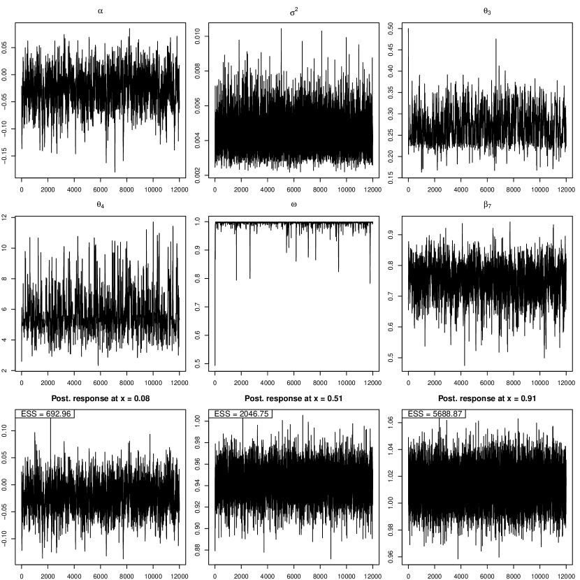
Figure 4: Traceplots of the NLFS(Hill) example fit in Figure 2, pane (a), correct subspace specification. The first 2000 samples were discarded as burn-in. Due to the correct subspace specification, there is strong shrinkage ($\omega=(1+\tau^{2})^{-1}$ close to 1). The effective sample size (ESS) was calculated based on the 10000 draws after discarding the first 2000 burn-in draws using the coda R-package [Plummer et al., 2006].

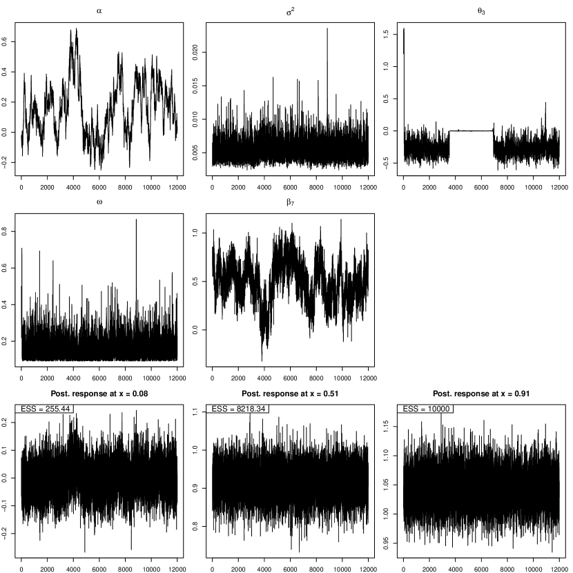
Figure 5: Traceplots of the NLFS(power) example fit in Figure 2, pane (b), subspace misspecification. The first 2000 samples were discarded as burn-in. Due to the subspace misspecification, there is little shrinkage ($\omega=(1+\tau^{2})^{-1}$ close to 0). Further, power exponent $\theta_{3}$ is stuck at 0 for a few thousand draws, and $\theta_{1}$, the intercept, seems highly correlated. Due to the misspecification and effectively no shrinkage, single parameters are not well identifiable and the whole response must be viewed to inspect convergence. The resulting response mixes well (bottom row). The effective sample size (ESS) was calculated based on the 10000 draws after discarding the first 2000 burn-in draws using the coda R-package [Plummer et al., 2006].

For all simulations, we use $k=15$ inner knots for the B-spline basis matrix. When MCMC sampling, we took 10,000 draws from the posterior, discarding the first 2000 samples as burn-in. Initial experiments indicated that this number of samples was adequate to estimate the posterior distribution. For the spline-based approaches (NLFS, B-spline, P-spline), we place a vague prior on the intercept term, $\theta_{1},$ defined in (8). Traceplots, of an NLFS fit with correctly and incorrectly specified subspaces, are given in the supplement (supplemental Figures 4 and 5) and show convergence.

4.2 Results

Figure 1 gives representative results of the simulation, where all results are provided in the supplement. Unsurprisingly, when the Hill model is the truth (Figure 1a), we observe the largest RMSE of 0.151 when fitting the misspecified parametric model (Param.(power)). Unlike the misspecified parametric fits, when the function space is misspecified in the NLFS approach (NLFS(power)), the RMSE is approximately one-third (0.046) that from fitting the misspecified parametric model, indicating the NLFS approach adjusts to the data. In this scenario, the NLFS(power) performance with mean RMSE of 0.046 was similar to that of the B-spline approach with mean RMSE of 0.042.

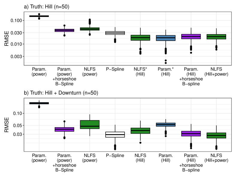
Figure 1: Representative root mean square error (RMSE) results of the simulation for the scenarios where the truth is Hill (a) or Hill + Downturn (b) and a medium noise level. Pane b represents the situation where a deviation of an unknown shape is the truth. All simulation results can be found in Tables S3 and S4. ^∗Correct model used in the model fit.

When the correct function space is assumed for the NLFS prior, the RMSE drops to 0.019 (Figure 1a), as low as that of the 0racle parametric fit. This demonstrates the adaptive shrinkage behavior of the NLFS approach in the case of correct subspace specification. Here, the NLFS approach effectively shrank towards the correctly assumed space for sample sizes as low as $n=50$, and performed similarly to the oracle parametric model fit. The P-spline approach receives no prior model or subspace specification but yields smooth splines. Consequently, its performance was in between the approach with misspecification and correct specification.

When the correct function space is assumed, the NLFS approach tended to outperform the parametric + horseshoe B-spline (PHBspline) approach. The PHBspline approach does not enforce an equally smooth, global shrinkage of all $\beta$ towards zero, especially when there are leverage points far from the observed mean.

When all assumed models or spaces are misspecified (Figure 1b), the NLFS approach was outperformed by the PHBspline approach for the same model misspecification, i.e., NLFS(power) was outperformed by param.(power) + horseshoe B-spline and NLFS(Hill) was outperformed by param.(Hill) + horseshoe B-spline. However, the NLFS approach in general has an advantage in misspecification scenarios due to its inherent flexibility to shrink toward combined function spaces. The NLFS(Hill+power) outperformed all other approaches in this scenario with a mean RMSE of 0.028. Only the P-spline approach came close, showing a slightly weaker performance with a mean RMSE of 0.030.

The NLFS prior appropriately shrinks into the correct space, giving equivalent fits to the parametric Hill model (Figure 2a). Correspondingly, the P-Spline smoothing approach estimate shows various artifactual bumps not evident in the NLFS approach. Even if the true model is the Hill model, the naive PHBspline approach produces an artifactual bump in the asymptote region that does not occur with the NLFS fit (Figure 2d). The NLFS approach and generic B-spline are equivalent when the model is misspecified (i.e., fits a model outside of the assumed space) (Figure 2b). The NLFS(Hill+power) approach fits a model outside of the Hill space (Figure 2c) and illustrates how shrinkage into combined subspaces can reduce misspecification errors involving minor deviations.

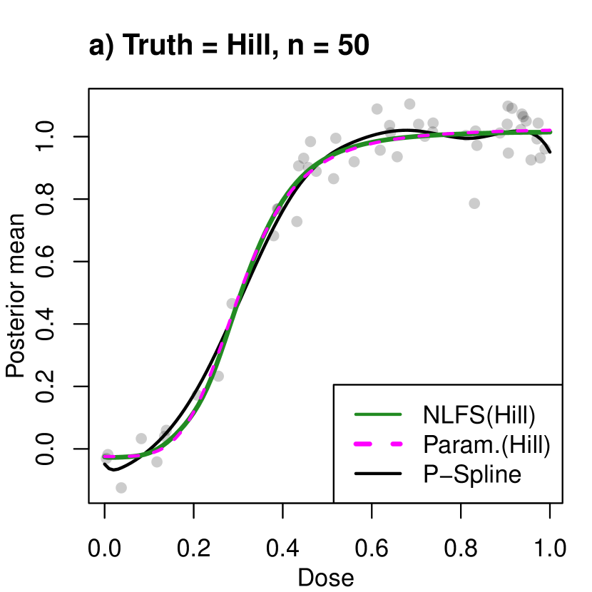
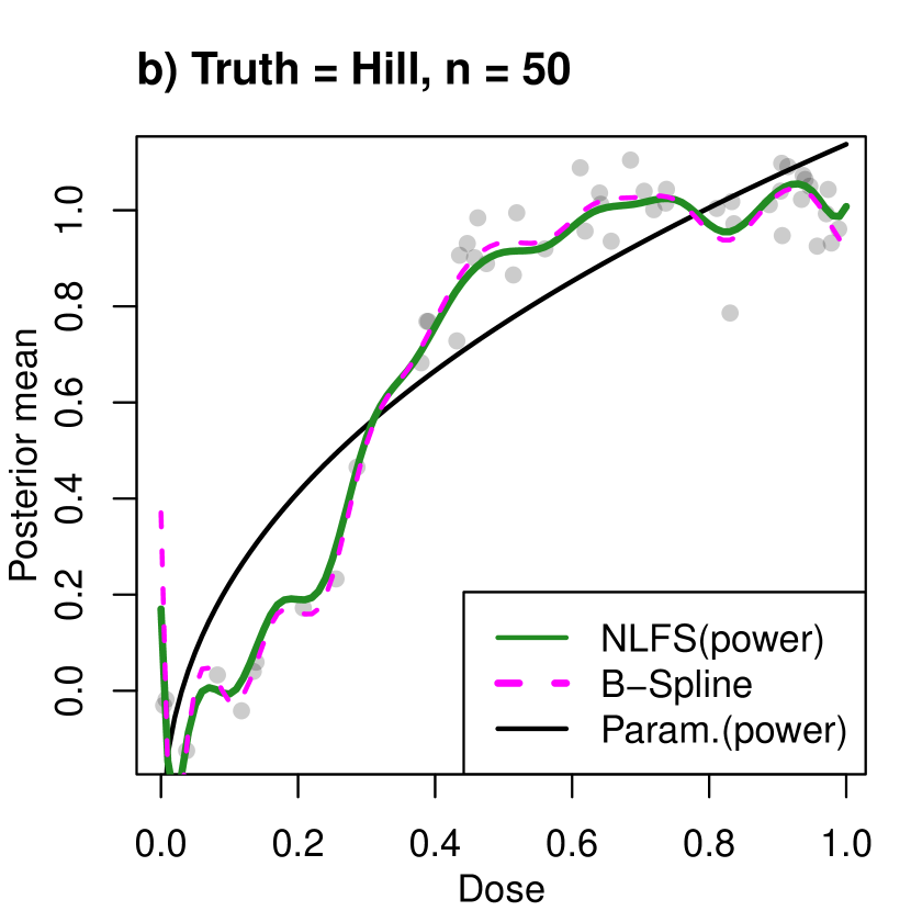
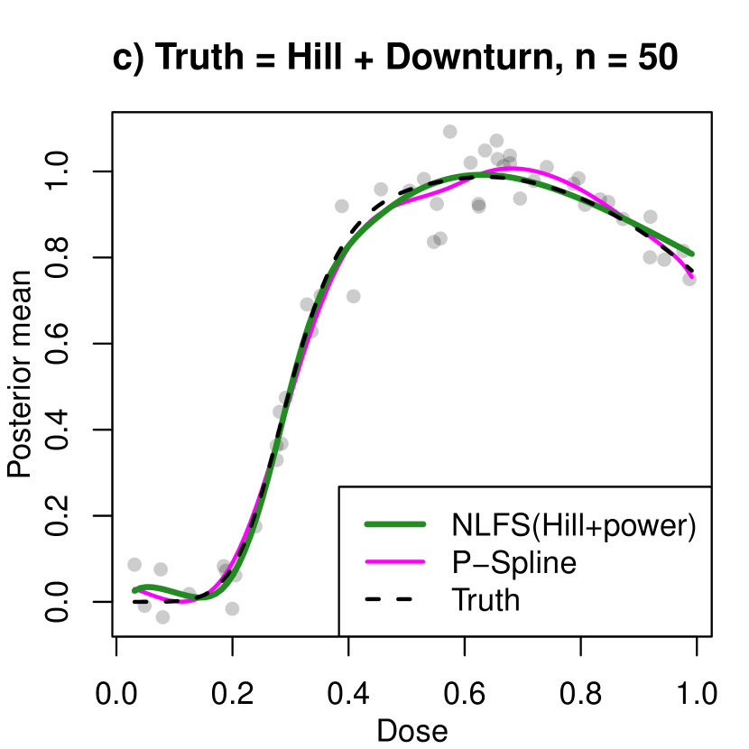
Figure 2: Posterior mean responses (a-d) and credible intervals (d) of representative simulation runs with median noise level ($\sigma^{2}=0.005$): (a) Oracle scenario. (b) misspecification scenario. (c) deviations of unknown shape. Combined subspace shrinkage reduces misspecification errors. (d) Comparison of credible intervals between NLFS and PHBspline in the Oracle scenario.

5 Real Data Example

We applied the proposed method on a testosterone data set collected by Kelsey et al. [2014]. They modeled total testosterone (TT) concentration in male participants dependent on age, to identify normal TT ranges at any age. TT levels are the result of highly complex physiological processes, mechanistic models are not available. TT is expected to increase during puberty, reach a maximum and possibly slowly decline with age, which is a sigmoidal assumption. Consequently, we a priori assume the Hill based shape through the NLFS prior.

Kelsey et al. [2014] collected data from 13 studies on TT by age, yielding $>$10.000 data points; they then fit 330 polynomial models and selected a single best parametric model based on the best $R^{2}$ with 5-fold cross-validation. Due to the large number of data points, spline smoothing approaches tend to produce local artifacts that are biologically unreasonable. The NLFS approach offers an alternative to extensive model comparisons while simultaneously incorporating knowledge on the curves shape.

For the analysis, we set

$$\theta_{3} \sim N(15,4),$$ (12)

$$\theta_{4} \sim LN(2.28,0.05).$$ (13)

Since testosterone levels increase during puberty, a priori we assume TT levels to reach half maximal levels (e.g., $\theta_{3}$) at approximately 15 years with a standard deviation of 2 years. For the steepness parameter, $\theta_{4},$ we set the log-mean to 2.28 and the log-variance to 0.05 implying that the actual mean and variance to be 10 and 5, respectively. We choose these values as we expect TT to increase rapidly upon the onset of puberty.

We fit our model to the slightly reduced data set of men of age 85 or younger (98.5% of original data) because of extreme variability in the approximately 150 observations above 85. To model the noise, we let $\sigma^{2}\sim C^{+}(0,1)$, to account for the large variance in the data.

The NLFS and parametric fit by Kelsey et al. [2014] are roughly sigmoidal (Figure 3). They both show a peak around age 19, followed by a slight descent that eventually plateaus. The NLFS approach notably predicts a larger mean testosterone level than the parametric model. The P-spline fit has a less pronounced peak TT around age 20 and has artifactual bumps that oscillate around the NLFS estimate. For each method, the observed RMSE values were 5.123 (NLFS), 5.154 (parametric), and 5.111 (P-spline) and therefore similar, but the three resulting model fits are visibly distinguishable. Arguably, the NLFS approach more appropriately models the mean than the P-spline due to the latter’s bumpiness. Further, NLFS estimates a higher mean TT level than the parametric model, which suggests there may be some underestimation of the mean TT when using a parametric approach.

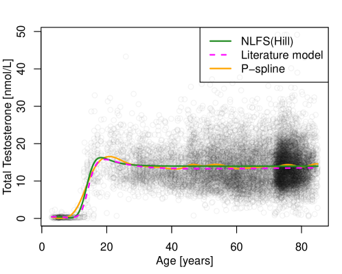
Figure 3: Comparison of the NLFS approach to a P-spline fit and the best parametric model selected by Kelsey et al. [2014]. For the P-spline and NLFS(Hill), the posterior mean is displayed. The parametric model by Kelsey is $\log_{10}(TT+1)=(a+cx+ex^{2}+gx^{3})/(1+bx+dx^{2}+fx^{2})$ with $a=0.04655$, $b=-0.05311$, $c=0.05123$, $-d=0.00793$, $e=-0.01222$, $f=0.00058$ and $g=0.00069$. For display, the model is backtransformed using $\exp(\log_{10}(TT+1)+\hat{\sigma}^{2}/2)$ where $\hat{\sigma}^{2}$ is the estimated residual variance.

6 Discussion

The NLFS prior enables adaptive shrinkage into a pre-specified non-linear function space but does not constrain the resulting function to be in that space if the data are not compatible with that a priori function space. This approach can be applied to function spaces defined by any twice differentiable function. Because such a setting is common, the NLFS approach balances adhering to prior assumptions and accounting for model misspecification.

The NLFS approach can shrink into a combined function space, thereby providing robustness against misspecification. This benefit is supported by simulation results, where NLFS combined function space prior outperformed all other methods under model misspecification. Defining such a prior is straightforward for the NLFS approach. Attempting to account for parametric misspecification by including a spline that shrinks to zero if the model is correctly specified can give artifactual features in the Oracle scenario. As a comparison, the NLFS prior gave slightly better RMSE results under the Oracle scenario, and provided more realistic curve fits without the artifactual features. Though NLFS with a misspecified single subspace performed slightly worse, adding subspaces in NLFS did not lead to a relevant performance loss compared to only including the correct model but also robustified NLFS against misspecification.

When modeling the TT data in Kelsey et al. [2014], the NLFS yielded a plausible non-parametric estimate that did not produce artifactual features. In this regard, NLFS provided equally reasonable mean estimates as the parametric model, while not requiring a model selection procedure on over 300 models.

Simulation results empirically show that NLFS correctly decides to either shrink towards the specified subspace, or remain unconstrained. Though we have not provided a theoretical proof, our simulation results suggest that the optimal, theoretical shrinkage properties given by Shin et al. [2020] approximately hold in the non-linear case. Because it performs similarly to an unsmoothed spline estimate, adding a smoothness penalty similar to the one proposed by Wiemann and Kneib [2021] for linear subspace shrinkage may be a promising extension.

The construction of NLFS assumes the independent variable to be continuously distributed, with a unique covariate value for each observation. In some biological applications, data are generated in a planned experimental setting, with multiple units treated at few distinct exposure levels. For such experiments, the exposure is typically a dose or concentration. Dose-response modeling is often performed in terms of a simple parametric Hill model fit, which can lead to misspecification errors that could be prevented using NLFS. Tailoring NLFS to a such a data structure is necessary. This can be done using a grid that defines the shrinkage locations, such that the shrinkage is independent of the few experimentally selected doses. Precisely, $\Phi_{\theta}$ would be evaluated at a grid instead of the observed exposure levels. This avoids a lack of shrinkage at basis functions that fall between exposure levels. This extension would yield more model parameters related to the construction of the grid. Another extension using a fully specified Gaussian processes is an alternative and would reduce hyperparameter choices on knot sequences and shrinkage grids. Another extension is to account for heteroscedasticity. For non-parametric Bayesian modeling, different methodologies can be applied, e.g. Dirichlet process priors. Other computational challenges in the NLFS approach relate to the derivatives. For example, using the Hill model, derivatives w.r.t. the non-linear parameters can be almost linearly dependent. Careful prior selection or expanding the shrinkage onto additional subspaces might soften this challenge.

Supporting Information

The code and data underlying this article are available on GitLab at
https://gitlab.tu-dortmund.de/functional_shrinkage/nonlinear_shrinkage.

Appendix A Tables

Table 1: Overview of method settings used in the simulation study.

	Algorithm	Assume	Shrinkage (Horseshoe prior)
1	NLFS	Hill	$a=b=0.5$
2	NLFS	Hill	$a=0.5,\,b=\exp(-k\log(n)/2)$
3	NLFS	Hill & power	$a=b=0.5$
4	NLFS	Hill & power	$a=0.5,\,b=\exp(-k\log(n)/2)$
5	NLFS	power	$a=b=0.5$
6	NLFS	power	$a=0.5,\,b=\exp(-k\log(n)/2)$
7	parametric	Hill	-
8	parametric	power	-
9	B-spline	-	-
10	P-spline	-	-
11	Parametric + B-spline	Hill	$a=b=0.5$
12	Parametric + B-spline	power	$a=b=0.5$

Table 2: Simulation setup summarized by the ADEMP principle.

Aim	Comparing proposed approach against existing approaches
Data generation	Dose-response models:
	- Hill: $h_{\theta}(x)=\frac{x^{\theta_{4}}}{\theta_{3}^{\theta_{4}}+x^{\theta_{4}}}$ ($\theta_{3}=0.3,\theta_{4}=6$)
	- Power: $h_{\theta}(x)=\theta_{1}x^{\theta_{2}}$, ($\theta_{2}=0.5$)
	- Hill + Downturn: $h_{\theta}(x)=h_{\theta}^{\text{Hill}}(x)+\mathbbm{1}_{[0.6,\infty)}(x)(-1.5(x-0.6)^{2})$ ($\theta_{3}=0.3,\theta_{4}=6$)
	Doses: Unif$\sim[0,1]$
	Sample sizes: $n\in\{50,100,200,500\}$
	Added noise: $\varepsilon\sim N(0,\sigma^{2})$, $\sigma^{2}\in\{0.005,0.05\}$
Estimand	Mean of posterior dose-response function estimate $f(x)$
Methods	Non-linear functional shrinkage (NLFS) ($\theta_{1}\sim N(0,1),\,\sigma^{2}\sim\text{IG}(0.001,0.001)$)
	- assuming Hill (NLFS (Hill))
	Priors: $\theta_{3}\sim N_{+}(0.5,0.05)$, $\theta_{4}\sim LN$ s.t. $\mathbb{E}(\theta_{4})=3$, $\mathbb{V}ar(\theta_{4})=3$
	- assuming power (NLFS (power))
	Priors: $\theta_{3}\sim N(0.5,0.25)$
	- assuming Hill and power (NLFS (Hill+power))
	Priors: As in NLFS(Hill) and NLFS(power)
	Parametric Bayesian fit (Param.) ($\theta_{1}\sim N(0,1),\,\log(\sigma^{2})\sim N(-1.75,1)$)
	- assuming Hill (Param.(Hill))
	Priors: $\theta_{3}\sim N_{+}(0.5,0.05)$, $\theta_{4}\sim LN$ s.t. $\mathbb{E}(\theta_{4})=3$, $\mathbb{V}ar(\theta_{4})=3$
	- assuming power (Param.(power))
	Priors: $\theta\sim N(0.5,0.25)$
	B-spline
	Priors: $\theta_{1}\sim N(0,1),\,\sigma^{2}\sim\text{IG}(0.001,0.001),\,\lambda^{2}\sim\text{IG}(0.001,0.001)$
	P-spline
	Priors: $\theta_{1}\sim N(0,1),\,\sigma^{2}\sim\text{IG}(0.001,0.001),\,\tau^{2}\sim\text{IG}(1,0.005)$
	Parametric + horseshoe B-spline
	$y=h_{\theta}(x)+\Phi(\beta)+\varepsilon$
	Priors:
	$\beta\sim N(0,\sigma^{2}\tau^{2}\text{diag}(\lambda_{1}^{2},\dots,\lambda_{k}^{2}))$
	$\tau\sim C^{+}(0,1)$, $\lambda_{j}\overset{\text{iid}}{\sim}C^{+}(0,1)$
	$\theta_{1}\sim N(0,1)$, $\theta_{2}\sim N(1.5,2)$ (Scaling)
	- assuming Hill (Param.(Hill) + B-spline))
	Prior: $\theta_{3}\sim N_{+}(0.5,0.05)$, $\theta_{4}\sim LN$ s.t. $\mathbb{E}(\theta_{4})=3$, $\mathbb{V}ar(\theta_{4})=3$
	- assuming power (Param.(power) + B-spline)
	Prior: $\theta\sim N(0.5,0.25)$
Performance	RMSE between posterior mean $\mathbb{E}(f(x)|d_{s}^{i})$ and true $g(x)$ evaluated at drawn doses $x\in[0,1]^{n}$

Table 3: Simulation results for $\sigma^{2}=0.005$ ($2\sigma=14.1\%$ of maximal effect) summarized by mean RMSE and corresponding standard deviation in parenthesis. OS means own slice and refers to setting $a$ and $b$ for the shrinkage parameters as suggested in Shin et al. [2020] whereas HC means Half Cauchy and refers to the standard horseshoe prior with $a=b=0.5$.

		n=50			n=100			n=200			n=500
	Method	Hill	power	Hill+down	Hill	power	Hill+down	Hill	power	Hill+down	Hill	power	Hill+down
1	NLFS(Hill), OS	0.019 (0.007)	0.027 (0.008)	0.037 (0.008)	0.014 (0.005)	0.017 (0.005)	0.028 (0.005)	0.009 (0.003)	0.011 (0.003)	0.024 (0.002)	0.006 (0.002)	0.008 (0.002)	0.017 (0.004)
2	NLFS(power), OS	0.046 (0.013)	0.018 (0.006)	0.053 (0.017)	0.031 (0.005)	0.013 (0.005)	0.031 (0.005)	0.023 (0.004)	0.009 (0.003)	0.022 (0.004)	0.015 (0.002)	0.006 (0.002)	0.015 (0.002)
3	NLFS(Hill+power), OS	0.021 (0.007)	0.022 (0.007)	0.028 (0.006)	0.015 (0.005)	0.015 (0.005)	0.023 (0.004)	0.01 (0.003)	0.011 (0.003)	0.018 (0.003)	0.007 (0.002)	0.007 (0.002)	0.011 (0.003)
4	NLFS(Hill), HC	0.019 (0.007)	0.022 (0.007)	0.033 (0.007)	0.014 (0.005)	0.015 (0.005)	0.027 (0.004)	0.01 (0.003)	0.011 (0.003)	0.024 (0.002)	0.006 (0.002)	0.008 (0.002)	0.015 (0.004)
5	NLFS(power), HC	0.046 (0.015)	0.017 (0.006)	0.054 (0.019)	0.03 (0.005)	0.012 (0.005)	0.03 (0.005)	0.021 (0.004)	0.009 (0.003)	0.022 (0.004)	0.013 (0.002)	0.006 (0.002)	0.013 (0.002)
6	NLFS(Hill&power), HC	0.021 (0.007)	0.021 (0.007)	0.028 (0.006)	0.015 (0.005)	0.015 (0.005)	0.023 (0.004)	0.01 (0.003)	0.011 (0.003)	0.018 (0.003)	0.007 (0.002)	0.007 (0.002)	0.011 (0.002)
7	param(Hill)	0.019 (0.007)	0.023 (0.005)	0.052 (0.008)	0.013 (0.005)	0.019 (0.004)	0.05 (0.005)	0.009 (0.003)	0.016 (0.002)	0.05 (0.003)	0.006 (0.002)	0.012 (0.001)	0.049 (0.002)
8	param(power)	0.151 (0.011)	0.015 (0.006)	0.18 (0.011)	0.152 (0.008)	0.011 (0.005)	0.18 (0.008)	0.154 (0.005)	0.008 (0.003)	0.181 (0.006)	0.154 (0.003)	0.005 (0.002)	0.182 (0.004)
9	bspline	0.042 (0.007)	0.042 (0.008)	0.042 (0.007)	0.032 (0.005)	0.033 (0.005)	0.032 (0.005)	0.023 (0.004)	0.024 (0.004)	0.023 (0.004)	0.014 (0.002)	0.014 (0.002)	0.014 (0.002)
10	pspline	0.03 (0.007)	0.026 (0.006)	0.03 (0.007)	0.022 (0.005)	0.019 (0.004)	0.022 (0.005)	0.016 (0.003)	0.015 (0.003)	0.016 (0.003)	0.011 (0.002)	0.01 (0.002)	0.011 (0.002)
11	param(Hill)+bspline	0.021 (0.007)	0.022 (0.006)	0.031 (0.006)	0.015 (0.005)	0.017 (0.004)	0.024 (0.005)	0.011 (0.003)	0.014 (0.003)	0.018 (0.003)	0.007 (0.002)	0.01 (0.002)	0.012 (0.002)
12	param(power)+bspline	0.038 (0.007)	0.019 (0.007)	0.04 (0.007)	0.029 (0.005)	0.013 (0.005)	0.03 (0.005)	0.021 (0.004)	0.009 (0.003)	0.022 (0.004)	0.013 (0.002)	0.006 (0.002)	0.014 (0.002)

Table 4: Simulation results for $\sigma^{2}=0.05$ ($2\sigma=44.7\%$ of maximal effect) summarized by mean RMSE and corresponding standard deviation in parenthesis. OS means own slice and refers to setting $a$ and $b$ for the shrinkage parameters as suggested in Shin et al. [2020] whereas HC means Half Cauchy and refers to the standard horseshoe prior with $a=b=0.5$.

		n=50			n=100			n=200			n=500
	Method	Hill	power	Hill+down	Hill	power	Hill+down	Hill	power	Hill+down	Hill	power	Hill+down
1	NLFS(Hill), OS	0.059 (0.021)	0.081 (0.021)	0.076 (0.017)	0.043 (0.015)	0.058 (0.015)	0.063 (0.012)	0.03 (0.01)	0.039 (0.011)	0.051 (0.009)	0.019 (0.007)	0.022 (0.007)	0.036 (0.007)
2	NLFS(power), OS	0.137 (0.015)	0.053 (0.019)	0.155 (0.022)	0.107 (0.023)	0.039 (0.014)	0.101 (0.024)	0.066 (0.012)	0.027 (0.011)	0.067 (0.012)	0.042 (0.007)	0.017 (0.007)	0.043 (0.007)
3	NLFS(Hill+power), OS	0.064 (0.021)	0.066 (0.021)	0.072 (0.019)	0.046 (0.015)	0.046 (0.015)	0.055 (0.014)	0.032 (0.01)	0.031 (0.011)	0.041 (0.01)	0.02 (0.007)	0.02 (0.007)	0.03 (0.006)
4	NLFS(Hill), HC	0.057 (0.02)	0.067 (0.02)	0.073 (0.017)	0.042 (0.015)	0.049 (0.015)	0.059 (0.013)	0.03 (0.01)	0.034 (0.011)	0.046 (0.01)	0.02 (0.007)	0.021 (0.007)	0.033 (0.006)
5	NLFS(power), HC	0.133 (0.016)	0.048 (0.02)	0.141 (0.026)	0.098 (0.021)	0.036 (0.015)	0.097 (0.019)	0.066 (0.013)	0.026 (0.011)	0.072 (0.014)	0.042 (0.007)	0.017 (0.007)	0.043 (0.008)
6	NLFS(Hill+power), HC	0.061 (0.02)	0.06 (0.019)	0.068 (0.019)	0.045 (0.015)	0.045 (0.015)	0.053 (0.014)	0.032 (0.01)	0.032 (0.011)	0.041 (0.01)	0.02 (0.007)	0.02 (0.007)	0.03 (0.006)
7	param(Hill)	0.063 (0.021)	0.054 (0.018)	0.082 (0.016)	0.043 (0.016)	0.042 (0.013)	0.066 (0.011)	0.03 (0.011)	0.033 (0.009)	0.058 (0.006)	0.019 (0.007)	0.024 (0.005)	0.053 (0.003)
8	param(power)	0.161 (0.012)	0.043 (0.019)	0.188 (0.012)	0.157 (0.008)	0.032 (0.014)	0.184 (0.009)	0.156 (0.005)	0.024 (0.01)	0.183 (0.006)	0.155 (0.003)	0.016 (0.007)	0.183 (0.004)
9	bspline	0.112 (0.02)	0.107 (0.022)	0.111 (0.02)	0.088 (0.014)	0.084 (0.014)	0.086 (0.014)	0.068 (0.01)	0.067 (0.01)	0.067 (0.01)	0.047 (0.006)	0.048 (0.006)	0.046 (0.006)
10	pspline	0.081 (0.019)	0.063 (0.017)	0.08 (0.019)	0.061 (0.014)	0.048 (0.013)	0.06 (0.013)	0.045 (0.01)	0.037 (0.009)	0.045 (0.01)	0.03 (0.006)	0.026 (0.006)	0.03 (0.006)
11	param(Hill)+bspline, HC	0.072 (0.021)	0.06 (0.02)	0.081 (0.019)	0.05 (0.016)	0.045 (0.014)	0.061 (0.014)	0.034 (0.011)	0.034 (0.01)	0.047 (0.009)	0.022 (0.007)	0.023 (0.006)	0.033 (0.006)
12	param(power)+bspline, HC	0.097 (0.019)	0.053 (0.02)	0.103 (0.019)	0.076 (0.014)	0.039 (0.015)	0.081 (0.014)	0.058 (0.01)	0.028 (0.01)	0.061 (0.01)	0.04 (0.006)	0.019 (0.007)	0.042 (0.006)

Appendix B Figures

Appendix C Proofs

Lemma 1: $P_{\theta}$ does not depend on linear parameters.

Proof.

Let $h(x,\theta)=\theta_{1}+\theta_{2}q(x,\theta_{3})$ be a twice differentiable function with $q$ non-linear in $\theta_{3}$. W.L.o.G. assume that $\theta_{3}\in\mathbb{R}$. Then

$$\dot{\text{H}}_{\theta}=\frac{\partial h(x,\theta)}{\partial\theta}=(1_{n}\quad\underbrace{q(x,\theta_{3})}_{:=c_{1}}\quad\theta_{2}\underbrace{\frac{\partial q(x,\theta_{3})}{\partial\theta_{3}}}_{:=c_{2}})=\underbrace{(1_{n}\quad c_{1}\quad c_{2})}_{:=H_{1}\in\mathbb{R}^{n\times 3}}\underbrace{\begin{pmatrix}1&0&0\\ 0&1&0\\ 0&0&\theta_{2}\end{pmatrix}}_{H_{2}\in\mathbb{R}^{3\times 3}}$$

and

$$P_{\theta} =\dot{\text{H}}_{\theta}(\dot{\text{H}}_{\theta}^{\top}\dot{\text{H}}_{\theta})^{-1}\dot{\text{H}}_{\theta}^{\top}$$

$$=H_{1}H_{2}(H_{2}H_{1}^{\top}H_{1}H_{2})^{-1}H_{2}H_{1}^{\top}$$

$$=H_{1}H_{2}H_{2}^{-1}(H_{1}^{\top}H_{1})^{-1}H_{2}^{-1}H_{2}H_{1}^{\top}$$

$$=H_{1}(H_{1}^{\top}H_{1})^{-1}H_{1}^{\top}$$

and $H_{1}$ does not depend on $\theta_{2}$. ∎∎

Appendix D Computation

The code to reproduce results is available at
https://gitlab.tu-dortmund.de/functional_shrinkage/nonlinear_shrinkage.

The non-linear functional shrinkage (NLFS) approach for the Hill model is implemented using a combination of Gibbs-, Metropolis-Hastings- and Slice sampling [Brooks et al., 2011, Neal, 2003]. We separately model the function intercept $\theta_{1}$.

Given the likelihood and priors

$$Y \sim N(\theta_{1}1_{n}+\Phi\beta,\sigma^{2}I_{n})$$

$$\sigma^{2} \sim\text{IG}(a_{\sigma},b_{\sigma}),\,\theta_{1}\sim N(\mu_{\theta_{1}},\sigma^{2}_{\theta_{1}})$$

$$\beta \sim N(0,\sigma^{2}\tau^{2}(\Phi^{\top}(I-P_{\theta})\Phi)^{-1})$$

$$\theta_{3} \sim N_{+}(\mu_{\theta_{3}},\sigma^{2}_{\theta_{3}}),\,\theta_{4}\sim LN(\mu_{\theta_{4}},\sigma^{2}_{\theta_{4}})$$

$$\omega =1/(1+\tau^{2})\sim\text{Beta}(a_{\omega},b_{\omega}),\,a_{\omega}=0.5,\,b_{\omega}=\exp(-\log(n)/2),$$

the sampler is summarized in Algorithm 1.

Algorithm 1 Non-linear functional shrinkage (NLFS)

1:Initialize: $\beta^{(1)},\sigma^{2(1)},\tau^{(1)},\omega^{(1)},\theta^{(1)}$

2:for $i:\,2\rightarrow B$ do

3:     Calculate $\dot{\text{H}}_{\theta^{(i-1)}}$

4:     Sample $\beta^{(i)}\sim p(\beta|\cdot)$ $\triangleright$ Conjugate

5:     Sample $\theta_{1}^{(i)}\sim p(\theta_{1}|\cdot)$ $\triangleright$ Conjugate

6:     Sample $\sigma^{2(i)}\sim p(\sigma^{2}|\cdot)$ $\triangleright$ Conjugate

7:     Sample $\omega^{(i)}\sim p(\omega|\cdot)$ $\triangleright$ Slice Sampler

8:     Sample Non-linear $\theta^{(i)}\sim p(\theta|\cdot)$ $\triangleright$ MH Sampler

9:end for

10:return All samples

Update $\beta$
We update $\beta$ using the full conditional posterior

$$\beta|\sigma^{2},\tau^{2},\theta,y\sim N(\mu_{\beta}^{\prime},\Sigma_{\beta}^{\prime})$$ (14)

where $\Sigma_{\beta}^{\prime}=\sigma^{2}(\Phi^{\top}\Phi+\tau^{2}\Phi^{\top}(I_{n}-P_{\theta})\Phi)^{-1}$ and $\mu_{\beta}^{\prime}=\sigma^{-2}\Sigma_{\beta}^{\prime}\Phi^{\prime}\tilde{y}$ and $\tilde{y}=y-1_{n}\theta_{1}$.

Update $\theta_{1}$

The intercept $\theta_{1}$ is updated using

$$\theta_{1}|\beta,\sigma^{2},y\sim N(\mu_{\theta_{1}}^{\prime},{\sigma^{2}_{\theta_{1}}}^{\prime})$$ (15)

where ${\sigma^{2}_{\theta_{1}}}^{\prime}=(\sigma^{2}\sigma^{2}_{\theta_{1}})(n\sigma^{2}_{\theta_{1}}+\sigma^{2})$ and $\mu_{\theta_{1}}^{\prime}=\sigma^{-2}{\sigma^{2}_{\theta_{1}}}^{\prime}1_{n}^{\top}(y-\Phi\beta)+\mu_{\theta_{1}}/\sigma^{2}_{\theta_{1}}$.

Update $\sigma^{2}$
The noise variance $\sigma^{2}$ is updated by

$$\sigma^{2}|\beta,\tau^{2},\theta\sim\text{IG}(a_{\sigma}^{\prime},b_{\sigma}^{\prime})$$ (16)

where $a_{\sigma}^{\prime}=(n+k)/2+a_{\sigma}$ and $b_{\sigma}^{\prime}=0.5(\text{RSS}+\tau^{-2}\beta^{\top}(\Phi^{\top}(I_{n}-P_{\theta})\Phi)\beta)+b_{\sigma}$ where $RSS={||y-(\theta_{1}1_{n}+\Phi\beta)||}_{2}^{2}$ is the residual sum of squares and $||.||_{2}$ is the Euclidean norm.

Update $\tau^{2}$
We update $\tau^{2}$ using a slice sampler [Neal, 2003] considering the posterior log likelihood

$$g(\tau)=\log(p(\tau|\beta,\sigma^{2},\theta))= (-k/2+b_{\omega}-0.5)\log(\tau^{2})$$ (17)

$$+(-a_{\omega}-b_{\omega})\log(1+\tau^{2})$$ (18)

$$+\left(-\frac{1}{2\sigma^{2}}\beta^{\top}\Phi^{\top}(I_{n}-P_{\theta})\Phi\beta\right)\tau^{-2}.$$ (19)

Note that we use $-k/2$ and not $-(k-d_{0})/2$ as in Shin et al. [2020] where $d_{0}$ is the rank of the (linear) projection matrix. We omit $-d_{0}$ as for the non-linear approach, there are no linear bases in $\dot{\text{H}}_{\theta}$ that are in $\Phi$ (because there is no intercept in $\Phi$) and hence the prior covariance matrix of $\beta$ is of full rank $k$. For a current $\tau_{0}$, calculate $v=g(\tau_{0}))$. Uniformly draw $\tilde{z}\sim U(0,\exp(v))$. For $z=\log(\tilde{z})$ define the slice $S_{z}=\{x:g(x)<g(z)\}$ and sample the next $\tau_{1}$ uniformly from $S_{z}$. For computational ease, we restrict $\tau^{2}$ to [0.001, 10].

The above sampling for the general $\omega\sim\text{Beta}(a_{\omega},b_{\omega})$ prior was primarily featured and labelled ’own slice’ (OC) in Table 3. We also considered a standard horseshoe (HS) prior ($a=b=0.5$). Details on its implementation are in Makalic and Schmidt [2015].

Update non-linear $\theta$
One only has to update the non-linear parameters of $\theta$, as $P_{\theta}$ only depends on the non-linear parameters. For the Hill model, the non-linear parameters are $\theta_{3}$ and $\theta_{4}$. We assume independence and separately update $\theta_{3}$ and $\theta_{4}$ using a Metropolis-Hastings sampler [Brooks et al., 2011] and explain the sampling for $\theta_{3}$.

Perform the three sampling steps

1. Draw a candidate $\theta_{3}^{(1)}$ from a proposal distribution $p_{\text{prop}}$using $\theta_{3}^{(0)}$

2. Calculate the hastings ratio

   $$\text{HR}=\frac{p(\theta_{3}^{(1)}|\cdot)p_{\text{prop}}(\theta_{3}^{(0)}|\theta_{3}^{(1)})}{p(\theta_{3}^{(0)}|\cdot)p_{\text{prop}}(\theta_{3}^{(1)}|\theta_{3}^{(0)})}.$$

3. Draw $u\sim\text{Unif}[0,1]$. If $\text{HR}>u$, accept $\theta_{3}^{(1)}$ as new draw. Otherwise, reject and consider $\theta_{3}^{(0)}$ as new draw.

For step (1), sample a new candidate $\theta_{3}^{(1)}$ from a proposal distribution, e.g. $N_{+}(\theta_{3}^{(0)},\sigma^{2}_{\text{prop}})$ where $\sigma^{2}_{\text{prop}}$ might be calculated as, e.g. the empirical variance of the latest 100 draws of $\theta_{3}$, or simply as $\sigma^{2}_{\text{prop}}=\sigma^{2}_{\theta_{3}}$. To sample $x$ from a truncated normal distribution with positive support, $x\sim N_{+}(\mu,\sigma^{2})$, calculate $l=P(X<0)$ where $X\sim N(\mu,\sigma^{2})$. Sample $u\sim\text{Unif}[l,1]$ and calculate $x=q_{\mu,\sigma^{2}}(u)$, the corresponding quantile.

For step (2), consider $\log(\text{HR})$ for computational stability:

$$\log(\text{HR})=\log(p(\theta_{3}^{(1)}|\cdot))-\log(p(\theta_{3}^{(0)}|\cdot))+\log(p_{\text{prop}}(\theta_{3}^{(0)}|\theta_{3}^{(1)}))-\log(p_{\text{prop}}(\theta_{3}^{(1)}|\theta_{3}^{(0)})).$$

For the fully conditional log posterior $\log(p(\theta|\cdot))$, we can integrate out $\beta$ to reduce the autocorrelation in the sampling. Since $p(\theta|\cdot)\propto p(y|\theta,\sigma^{2},\tau^{2})p(\theta)$ and

$$y|\theta,\sigma^{2},\tau^{2}\sim N(\mathbb{E}(\Phi\beta+\varepsilon),\text{Cov}(\Phi\beta+\varepsilon)),$$

we use $y|\theta,\sigma^{2},\tau^{2}\sim N(0,\Sigma_{y})$ with $\Sigma_{y}=\sigma^{2}\tau^{2}\Phi(\Phi^{\top}(I-P_{\theta})\Phi)^{-1}\Phi^{\top}+\sigma^{2}I_{n}$.

References

- Alvarez et al. [2013] M. A. Alvarez, D. Luengo, and N. D. Lawrence. Linear latent force models using gaussian processes. IEEE transactions on pattern analysis and machine intelligence, 35(11):2693–2705, 2013.
- Brezger and Steiner [2008] A. Brezger and W. J. Steiner. Monotonic regression based on bayesian p–splines. Journal of Business & Economic Statistics, 26(1):90–104, 2008. doi: 10.1198/073500107000000223. URL https://doi.org/10.1198/073500107000000223.
- Brooks et al. [2011] S. Brooks, A. Gelman, G. Jones, and X.-L. Meng. Handbook of markov chain monte carlo. CRC press, 2011.
- Carl [2001] D. Carl. A practical guide to splines. Springer, 2001.
- Carvalho et al. [2010] C. M. Carvalho, N. G. Polson, and J. G. Scott. The horseshoe estimator for sparse signals. Biometrika, 97(2):465–480, 2010.
- Chen et al. [2022] J. Chen, Z. Chen, C. Zhang, and C. Jeff Wu. Apik: Active physics-informed kriging model with partial differential equations. SIAM/ASA Journal on Uncertainty Quantification, 10(1):481–506, 2022.
- Golightly and Wilkinson [2011] A. Golightly and D. J. Wilkinson. Bayesian parameter inference for stochastic biochemical network models using particle markov chain monte carlo. Interface focus, 1(6):807–820, 2011.
- Goutelle et al. [2008] S. Goutelle, M. Maurin, F. Rougier, X. Barbaut, L. Bourguignon, M. Ducher, and P. Maire. The hill equation: a review of its capabilities in pharmacological modelling. Fundamental & clinical pharmacology, 22(6):633–648, 2008.
- Gunn and Dunson [2005] L. H. Gunn and D. B. Dunson. A transformation approach for incorporating monotone or unimodal constraints. Biostatistics, 6(3):434–449, 2005.
- Hill [1910] A. V. Hill. The possible effects of the aggregation of the molecules of hemoglobin on its dissociation curves. The Journal of Physiology, 40:iv–vii, 1910.
- Hoerl and Kennard [1970] A. E. Hoerl and R. W. Kennard. Ridge regression: Biased estimation for nonorthogonal problems. Technometrics, 12(1):55–67, 1970.
- Huang et al. [2006] Y. Huang, D. Liu, and H. Wu. Hierarchical bayesian methods for estimation of parameters in a longitudinal hiv dynamic system. Biometrics, 62(2):413–423, 2006.
- Kelsey et al. [2014] T. W. Kelsey, L. Q. Li, R. T. Mitchell, A. Whelan, R. A. Anderson, and W. H. B. Wallace. A validated age-related normative model for male total testosterone shows increasing variance but no decline after age 40 years. PloS one, 9(10):e109346, 2014.
- Köllmann et al. [2014] C. Köllmann, B. Bornkamp, and K. Ickstadt. Unimodal regression using bernstein–schoenberg splines and penalties. Biometrics, 70(4):783–793, 2014.
- Lang and Brezger [2004] S. Lang and A. Brezger. Bayesian p-splines. Journal of computational and graphical statistics, 13(1):183–212, 2004.
- Lunn et al. [2002] D. J. Lunn, N. Best, A. Thomas, J. Wakefield, and D. Spiegelhalter. Bayesian analysis of population pk/pd models: general concepts and software. Journal of pharmacokinetics and pharmacodynamics, 29:271–307, 2002.
- Makalic and Schmidt [2015] E. Makalic and D. F. Schmidt. A simple sampler for the horseshoe estimator. IEEE Signal Processing Letters, 23(1):179–182, 2015.
- Mesarovic et al. [2004] D. Mesarovic, Mihajlo, S. Sreenath, and J. Keene. Search for organising principles: understanding in systems biology. Systems biology, 1(1):19–27, 2004.
- Meyer [2008] M. C. Meyer. Inference using shape-restricted regression splines. The Annals of Applied Statistics, 2(3):1013–1033, 2008. ISSN 19326157. URL http://www.jstor.org/stable/30245118.
- Meyer et al. [2011] M. C. Meyer, A. J. Hackstadt, and J. A. Hoeting. Bayesian estimation and inference for generalised partial linear models using shape-restricted splines. Journal of Nonparametric Statistics, 23(4):867–884, 2011.
- Morris et al. [2019] T. P. Morris, I. R. White, and M. J. Crowther. Using simulation studies to evaluate statistical methods. Statistics in medicine, 38(11):2074–2102, 2019.
- Neal [2003] R. M. Neal. Slice sampling. The annals of statistics, 31(3):705–767, 2003.
- Plummer et al. [2006] M. Plummer, N. Best, K. Cowles, and K. Vines. Coda: Convergence diagnosis and output analysis for MCMC. R News, 6(1):7–11, 2006. URL https://journal.r-project.org/archive/.
- Seber and Wild [2003] G. A. Seber and C. J. Wild. Nonlinear regression. hoboken. New Jersey: John Wiley & Sons, 62(63):1238, 2003.
- Shin et al. [2020] M. Shin, A. Bhattacharya, and V. E. Johnson. Functional horseshoe priors for subspace shrinkage. Journal of the American Statistical Association, 115(532):1784–1797, 2020.
- Shively et al. [2009] T. S. Shively, T. W. Sager, and S. G. Walker. A bayesian approach to non-parametric monotone function estimation. Journal of the Royal Statistical Society. Series B (Statistical Methodology), 71(1):159–175, 2009.
- Shively et al. [2011] T. S. Shively, S. G. Walker, and P. Damien. Nonparametric function estimation subject to monotonicity, convexity and other shape constraints. Journal of Econometrics, 161(2):166–181, 2011.
- Šimon [2005] P. Šimon. Considerations on the single-step kinetics approximation. Journal of Thermal Analysis and Calorimetry, 82(3):651–657, 2005.
- Tibshirani [1996] R. Tibshirani. Regression shrinkage and selection via the lasso. Journal of the Royal Statistical Society: Series B (Methodological), 58(1):267–288, 1996.
- Titsias et al. [2012] M. K. Titsias, A. Honkela, N. D. Lawrence, and M. Rattray. Identifying targets of multiple co-regulating transcription factors from expression time-series by bayesian model comparison. BMC systems biology, 6:1–21, 2012.
- Wheeler et al. [2014] M. W. Wheeler, D. B. Dunson, S. P. Pandalai, B. A. Baker, and A. H. Herring. Mechanistic hierarchical gaussian processes. Journal of the American Statistical Association, 109(507):894–904, 2014.
- Wheeler et al. [2017] M. W. Wheeler, D. B. Dunson, and A. H. Herring. Bayesian local extremum splines. Biometrika, 104(4):939–952, 2017.
- Wiemann and Kneib [2021] P. Wiemann and T. Kneib. Adaptive shrinkage of smooth functional effects towards a predefined functional subspace. arXiv preprint arXiv:2101.05630, 2021.