Neural Dueling Bandits

Abstract

Contextual dueling bandit is used to model the bandit problems, where a learner’s goal is to find the best arm for a given context using observed noisy preference feedback over the selected arms for the past contexts. However, existing algorithms assume the reward function is linear, which can be complex and non-linear in many real-life applications like online recommendations or ranking web search results. To overcome this challenge, we use a neural network to estimate the reward function using preference feedback for the previously selected arms. We propose upper confidence bound- and Thompson sampling-based algorithms with sub-linear regret guarantees that efficiently select arms in each round. We then extend our theoretical results to contextual bandit problems with binary feedback, which is in itself a non-trivial contribution. Experimental results on the problem instances derived from synthetic datasets corroborate our theoretical results.

1 Introduction

Contextual dueling bandits (or preference-based bandits) [1, 2, 3] is a sequential decision-making framework that is widely used to model the contextual bandit problems [4, 5, 6, 7, 8] in which a learner’s goal is to find an optimal arm by sequentially selecting a pair of arms (also refers as a duel) and then observing noisy preference feedback (i.e., one arm is preferred over another) for the selected arms. Contextual dueling bandits has many real-life applications, e.g., online recommendation, ranking web search, comparing two text responses generated from LLMs, and rating two restaurants/ movies, especially in the applications where it is easier to observe preference between two arms than knowing the absolute reward for the selected arm. The preference feedback between two arms is often assumed to follow the Bradley-Terry-Luce (BTL) model [2, 10, 11] in which the probability of preferring an arm is proportional to the exponential of its reward.

Since the number of contexts (e.g., users of online platforms) and arms (e.g., movies/search results to recommend) can be very large (or infinite), the reward of an arm is assumed to be parameterized by an unknown function, e.g., a linear function [1, 2, 3]. However, the reward function may not always be linear in practice. To overcome this challenge, this paper parameterizes the reward function via a non-linear function, which needs to be estimated using the available preference feedback for selected arms. To achieve this, we can estimate the non-linear function by using either a Gaussian processes [12, 13, 14] or a neural network [7, 8]. However, due to the limited expressive power of the Gaussian processes, it fails when optimizing highly complex functions. In contrast, neural networks (NNs) possess strong expressive power and can model highly complex functions [15, 16].

In this paper, we first introduce the problem setting of neural dueling bandits, in which we use a neural network to model the unknown reward function in contextual dueling bandits. As compared to the existing work on neural contextual bandits [7, 8], we have to use cross-entropy loss due to binary preference feedback. We then propose the first two neural dueling bandit algorithms based on, respectively, upper confidence bound (UCB) [4, 5, 7, 17, 18, 19] and Thompson sampling (TS) [8, 14, 20, 21] (in Section 3.1). Under mild assumptions, we derive an upper bound on the estimation error of the difference between the reward values of any pair of arms (1), which is valid as long as the neural network is sufficiently wide. This result provides a theoretical assurance of the quality of our trained neural network using the preference feedback. Based on the theoretical guarantee on the estimation error, we derive upper bounds on the cumulative regret of both of our algorithms (2 and 3), which are sub-linear under some mild conditions. Our regret upper bounds lead to a number of interesting and novel insights (more details in Section 3.2).

Interestingly, our theoretical results provide novel theoretical insights regarding the reinforcement learning with human feedback (RLHF) algorithm (Section 4). Specifically, our 1 naturally provides a theoretical guarantee on the quality of the learned reward model in terms of its accuracy in estimating the reward differences between pairs of responses. As a special case, we extend our results to neural contextual bandit problems with binary feedback in Section 5, which is itself of independent interest. Finally, we empirically validate the different performance aspects of our proposed algorithms in Section 6 using problem instances derived from synthetic datasets.

Related work.  Learning from pairwise or $K$-wise comparisons has been thoroughly explored in the literature. In the context of dueling bandits, the focus is on minimizing regret using preference feedback [22, 23, 24, 25, 26, 27, 28, 29, 30, 31, 32, 33, 34]. We refer the readers to [35] for a detailed survey on dueling bandits. The closest work to ours is contextual dueling bandits [1, 2, 3, 36, 37], but they only consider the linear reward function, which we extend to the non-linear reward functions.

2 Problem Setting

Contextual dueling bandits.  We consider a contextual dueling bandit problem in which a learner selects two arms (also refers as a duel) for a given context and observes preference feedback over arms. The learner’s goal is to find the best arm for each context. Let $\mathcal{C}\subset\mathbb{R}^{d_{c}}$ be the context set and $\mathcal{A}\subset\mathbb{R}^{d_{a}}$ be finite arm set, where $d_{c}\geq 1$ and $d_{a}\geq 1$. At the beginning of round $t$, the environment generates a context $c_{t}\in\mathcal{C}$ and the learner selects two arms (i.e., $a_{t,1}$, and $a_{t,2}$) from the finite arm set $\mathcal{A}$. After selecting two arms, the learner observes stochastic preference feedback $y_{t}$ for the selected arms, where $y_{t}=1$ implies the arm $a_{t,1}$ is preferred over arm $a_{t,2}$ and $y_{t}=0$ otherwise. We assume that the preference feedback depends on an unknown non-linear reward function $f:\mathcal{C}\times\mathcal{A}\rightarrow\mathbb{R}$. For brevity, we denote the set of all context-arm feature vectors in the round $t$ by $\mathcal{X}_{t}\subset\mathbb{R}^{d}$ and use $x_{t}^{a}$ to represent the context-arm feature vector for context $c_{t}$ and an arm $a$.

Stochastic preference model.  We assume the preference has a Bernoulli distribution that follows the Bradley-Terry-Luce (BTL) model [10, 11], which is commonly used in the dueling bandits [1, 2, 3]. Under BTL preference model, the probability that the first selected arm $(x_{t,1})$ is preferred over the second selected arm $(x_{t,2})$ for the given reward function $f$ is given by

$$\mathbb{P}\left\{x_{t,1}\succ x_{t,2}\right\}=\mathbb{P}\left\{y_{t}=1|x_{t,1},x_{t,2}\right\}=\frac{\exp\left(f(x_{t,1})\right)}{\exp\left(f(x_{t,1})\right)+\exp\left(f(x_{t,2})\right)}=\mu\left(f(x_{t,1})-f(x_{t,2})\right).$$

where $x_{1}\succ x_{2}$ denotes that $x_{t,1}$ is preferred over $x_{t,2}$, $\mu(x)=1/(1+\mathrm{e}^{-x})$ is the logistic function, and $f(x_{t,i})$ is the latent reward of the $i$-th selected arm for the given context $c_{t}$. We need the following standard assumptions on function $\mu$ (also known as a link function in the literature [2, 19]):

Assumption 1.

• $\kappa_{\mu}\doteq\inf_{x,x^{\prime}\in\mathcal{X}}\dot{\mu}(f(x)-f(x^{\prime}))>0$ for all pairs of context-arm.

• The link function $\mu:\mathbb{R}\rightarrow[0,1]$ is continuously differentiable and Lipschitz with constant $L_{\mu}$. For logistic function, $L_{\mu}\leq 1/4$.

Performance measure.  After selecting two arms, denoted by $x_{t,1}$ and $x_{t,2}$, in round $t$, the learner incurs an instantaneous regret. There are two common notions of instantaneous regret in the dueling bandits setting, i.e., average instantaneous regret: $r_{t}^{a}\doteq f(x_{t}^{\star})-\left({f(x_{t,1})+f(x_{t,2})}\right)/{2}$, and weak instantaneous regret: $r_{t}^{w}\doteq f(x_{t}^{\star})-\max\left\{f(x_{t,1}),f(x_{t,2})\right\}$, where $x_{t}^{\star}=\arg\!\max_{x\in\mathcal{X}_{t}}f(x)$ denotes the best arm for a given context that maximizes the value of the underlying reward function. After observing preference feedback for $T$ pairs of arms, the cumulative regret (or regret, in short) of a sequential policy is given by $\mathfrak{R}_{T}^{\tau}=\sum_{t=1}^{T}r_{t}^{\tau},$ where $\tau\doteq\{a,w\}$. Any good policy should have sub-linear regret, i.e., $\lim_{T\to\infty}{\mathfrak{R}_{T}^{\tau}}/T=0.$ A policy with a sub-linear regret implies that the policy will eventually find the best arm and recommend only the best arm in the duel for the given contexts.

3 Neural Dueling Bandits

Having a good reward function estimator is the key for any contextual bandit algorithm to achieve good performance, i.e., smaller regret. As the underlying reward function is complex and non-linear, we use fully connected neural networks [7, 8] to estimate the reward function only using the preference feedback. Using this estimated reward function, we propose two algorithms based on the upper confidence bound and Thomson sampling with sub-linear regret guarantees.

Reward function estimation using neural network.

To estimate the unknown reward function $f$, we use a fully connected neural network (NN) with depth $L\geq 2$, the width of hidden layer $m$, and ReLU activations as done in [7] and [8]. Let $h(x;\theta)$ represent the output of a full-connected neural network with parameters $\theta$ for context-arm feature vector $x$, which is defined as follows:

$$h(x;\theta)=\boldsymbol{W}_{L}\text{ReLU}\left(\boldsymbol{W}_{L-1}\text{ReLU}\left(\cdots\text{ReLU}\left(\boldsymbol{W}_{1}x\right)\right)\right),$$

where $\text{ReLU}(x)\doteq\max\{x,0\}$, $\boldsymbol{W}_{1}\in\mathbb{R}^{m\times d}$, $\boldsymbol{W}_{l}\in\mathbb{R}^{m\times m}$ for $2\leq l<L$, $\boldsymbol{W}_{L}\in\mathbb{R}^{m\times 1}$. We denote the parameters of NN by $\theta=\left(\text{vec}\left(\boldsymbol{W}_{1}\right);\cdots\text{vec}\left(\boldsymbol{W}_{L}\right)\right)$, where $\text{vec}\left(A\right)$ converts a $M\times N$ matrix $A$ into a $MN$-dimensional vector. We use $m$ to denote the width of every layer of the NN, use $p$ to represent the total number of NN parameters, i.e., $p=dm+m^{2}(L-1)+m$, and use $g(x;\theta)$ to denote the gradient of $h(x;\theta)$ with respect to $\theta$.

The arms selected by the learner for context received in round $s$ is denoted by $x_{s,1},x_{s,2}\in\mathcal{X}_{s}$ and the observed stochastic preference feedback is denoted by $y_{s}=\mathbbmss{1}{\left(x_{s,1}\succ x_{s,2}\right)}$, which is equal to $1$ if the arm $x_{s,1}$ is preferred over the arm $x_{s,2}$ and $0$ otherwise. At the beginning of round $t$, we use the current history of observations $\left\{(x_{s,1},x_{s,2},y_{s})\right\}_{s=1}^{t-1}$ to train the neural network (NN) using gradient descent to minimize the following loss function:

$$\mathcal{L}_{t}(\theta)=-\frac{1}{m}\sum^{t-1}_{s=1}\Big{[}\log\mu\left((-1)^{1-y_{s}}\left[h(x_{s,1};\theta)-h(x_{s,2};\theta)\right]\right)\Big{]}+\frac{1}{2}\lambda\left\|\theta-\theta_{0}\right\|^{2}_{2},$$ (1)

Here $\theta_{0}$ represents the initial parameters of the NN, and we initialize $\theta_{0}$ following the standard practice of neural bandits [7, 8] (refer to Algorithm 1 in [8] for details). Here, minimizing the first term in the loss function (i.e., the term involving the summation from $t-1$ terms) corresponds to the maximum log likelihood estimate (MLE) of the parameters $\theta$. Next, we develop algorithms that use the trained NN with parameter $\theta_{t}$ to select the best arms (duel) for each context.

3.1 Neural dueling bandit algorithms

With the trained NN as an estimate for the unknown reward function, the learner has to decide which two arms (or duel) must be selected for the subsequent contexts. We use UCB- and TS-based algorithms that handle the exploration-exploitation trade-off efficiently.

UCB-based algorithm.  Using upper confidence bound for dealing with the exploration-exploitation trade-off is common in many sequential decision-making problems [2, 7, 17]. We propose a UCB-based algorithm named NDB-UCB, which works as follows: At the beginning of the round $t$, the algorithm trains the NN using available observations. After receiving the context, it selects the first arm greedily (i.e., by maximizing the output of the trained NN with parameter $\theta_{t}$) as follows:

$$x_{t,1}=\arg\max_{x\in\mathcal{X}_{t}}h(x;\theta_{t}).$$ (2)

NDB-UCB Algorithm for Neural Dueling Bandit based on Upper Confidence Bound

1:  Tuning parameters: $\delta\in(0,1)$, $\lambda>0$, and $m>0$

2:  for $t=1,\ldots,T$ do

3:     Train the NN using $\left\{(x_{s,1},x_{s,2},y_{s})\right\}_{s=1}^{t-1}$ by minimizing the loss function defined in Eq. 1

4:     Receive a context and $\mathcal{X}_{t}$ denotes the corresponding context-arm feature vectors

5:     Select $x_{t,1}=\arg\max_{x\in\mathcal{X}_{t}}h(x;\theta_{t})$ as given in Eq. 2)

6:     Select $x_{t,2}=\arg\max_{x\in\mathcal{X}_{t}}\left[h(x;\theta_{t})+\nu_{T}\sigma_{t-1}(x,x_{t,1})\right]$ (as given in Eq. 3)

7:     Observe preference feedback $y_{t}=\mathds{1}_{\left\{x_{t,1}\succ x_{t,2}\right\}}$

8:  end for

Next, the second arm $x_{t,2}$ is selected optimistically, i.e., by maximizing the UCB value:

$$x_{t,2}=\arg\max_{x\in\mathcal{X}_{t}}\left[h(x;\theta_{t})+\nu_{T}\sigma_{t-1}(x,x_{t,1})\right],$$ (3)

where $\nu_{T}\doteq(\beta_{T}+B\sqrt{\lambda/\kappa_{\mu}}+1)\sqrt{\kappa_{\mu}/\lambda}$ in which $\beta_{T}\doteq\frac{1}{\kappa_{\mu}}\sqrt{\widetilde{d}+2\log(1/\delta)}$ and $\widetilde{d}$ is the effective dimension. We define the effective dimension in Section 3.2 (see Eq. 4). We define

$$\sigma_{t-1}^{2}(x_{1},x_{2})\doteq\frac{\lambda}{\kappa_{\mu}}\left\|\frac{1}{\sqrt{m}}(\varphi(x_{1})-\varphi(x_{2}))\right\|^{2}_{V_{t-1}^{-1}},$$

where $V_{t}\doteq\sum_{s=1}^{t}\varphi^{\prime}(x_{s})\varphi^{\prime}(x_{s})^{\top}\frac{1}{m}+\frac{\lambda}{\kappa_{\mu}}\mathbf{I}$. Here, $\varphi^{\prime}(x_{s})\doteq\varphi(x_{s,1})-\varphi(x_{s,2})=g(x_{s,1};\theta_{0})-g(x_{s,2};\theta_{0})$ and $g(x;\theta_{0})/\sqrt{m}$ is used as the random features approximation for context-arm feature vector $x$. Intuitively, after the first arm $x_{t,1}$ is selected, a larger $\sigma_{t-1}^{2}(x,x_{t,1})$ indicates that $x$ is very different from $x_{t,1}$ given the information of the previously selected pairs of arms. Hence, the second term in Eq. 3 encourages the second selected arm to be different from the first arm.

TS-based algorithm.

Thompson sampling [3, 21] selects an arm according to its probability of being the best. Many works [3, 14, 21, 38] have shown that TS is empirically superior than to its counterpart UCB-based bandit algorithms. Therefore, in addition, we also propose another algorithm based on TS named NDB-TS, which works similarly to NDB-UCB except that the second arm $x_{t,2}$ is selected differently. To select the second arm $x_{t,2}$, for every arm $x\in\mathcal{X}_{t}$, it firstly samples a reward $r_{t}(x)\sim\mathcal{N}\left(h(x;\theta_{t})-h(x_{t,1};\theta_{t}),\nu_{T}^{2}\sigma_{t-1}^{2}(x,x_{t,1})\right)$ and then selects the second arm as $x_{t,2}={\arg\max}_{x\in\mathcal{X}_{t}}{r}_{t}(x)$.

3.2 Regret analysis

Let $K$ denote the finite number of available arms in each round, $\mathbf{H}$ denote the NTK matrix for all $T\times K$ context-arm feature vectors in the $T$ rounds, and $h=\left(f(x_{1}^{1}),\ldots,f(x_{T}^{K})\right)$. The NTK matrix $\mathbf{H}$ definition is adapted to our setting from Definition 4.1 of [7]. We now introduce the assumptions needed for our regret analysis, all of which are standard assumptions in neural bandits [7, 8].

Assumption 2.

Without loss of generality, we assume that

• the reward function is bounded: $|f(x)|\leq 1,\forall x\in\mathcal{X}_{t},t\in[T]$,

• there exists $\lambda_{0}>0$ s.t. $\mathbf{H}\succeq\lambda_{0}I$, and

• all context-arm feature vectors satisfy $\left\|x\right\|_{2}=1$ and $[x]_{j}=[x]_{j+d/2}$, $\forall x\in\mathcal{X}_{t},\forall t\in[T]$.

The last assumption in 2 above, together with the way we initialize $\theta_{0}$ (i.e., following standard practice in neural bandits [7, 8]), ensures that $h(x;\theta_{0})=0,\forall x\in\mathcal{X}_{t},\forall t\in[T]$.

Let $\mathbf{H}^{\prime}\doteq\sum_{s=1}^{T}\sum_{(i,j)\in C^{K}_{2}}z^{i}_{j}(s)z^{i}_{j}(s)^{\top}\frac{1}{m}$, in which $z^{i}_{j}(s)=\varphi(x_{s,i})-\varphi(x_{s,j})$ and $C^{K}_{2}$ denotes all pairwise combinations of $K$ arms. We now define the effective dimension as follows:

$$\widetilde{d}=\log\det\left(\frac{\kappa_{\mu}}{\lambda}\mathbf{H}^{\prime}+\mathbf{I}\right).$$ (4)

Compared to the previous works on neural bandits, our definition of $\widetilde{d}$ features extra dependencies on $\kappa_{\mu}$. Moreover, our $\mathbf{H}^{\prime}$ contains $T\times K\times(K-1)$ contexts, which is more than the $T\times K$ contexts of [7] and [8]. Hence, our $\widetilde{d}$ is expected to be generally larger than their standard effective dimension.

Note that placing an assumption on $\widetilde{d}$ above is analogous to the assumption on the eigenvalue of the matrix $M_{t}$ in the work on linear dueling bandits [2]. For example, in order for our final regret bound to be sub-linear, we only need to assume that $\widetilde{d}=\widetilde{O}(\sqrt{T})$, which is analogous to the assumption from [2]: $\sum^{T}_{t=\tau+1}\lambda_{\min}^{-1/2}(M_{t})\leq c\sqrt{T}$.

A key step in our proof is that minimizing the loss function Eq. 1 allows us to achieve the following:

$$\frac{1}{m}\sum_{s=1}^{t-1}\left(\mu\left(h(x_{s,1};\theta_{t})-h(x_{s,2};\theta_{t})\right)-y_{s}\right)(g(x_{s,1};\theta_{t})-g(x_{s,2};\theta_{t}))+\lambda(\theta_{t}-\theta_{0})=0.$$ (5)

We use the above fact to prove our following result, which is equivalent to the confidence ellipsoid results used in the existing bandit algorithms [19].

Theorem 1.

Let $\delta\in(0,1)$, $\varepsilon^{\prime}_{m,t}\doteq C_{2}m^{-1/6}\sqrt{\log m}L^{3}\left(\frac{t}{\lambda}\right)^{4/3}$ for some absolute constant $C_{2}>0$. As long as $m\geq\text{poly}(T,L,K,1/\kappa_{\mu},L_{\mu},1/\lambda_{0},1/\lambda,\log(1/\delta))$, then with probability of at least $1-\delta$,

$$|\left[f(x)-f(x^{\prime})\right]-\left[h(x;\theta_{t})-h(x^{\prime};\theta_{t})\right]|\leq\nu_{T}\sigma_{t-1}(x,x^{\prime})+2\varepsilon^{\prime}_{m,t},$$

for all $x,x^{\prime}\in\mathcal{X}_{t},t\in[T]$.

The detailed proof of 1 and all other missing proofs are given in the Appendix. Note that as long as the width $m$ of the NN is large enough (i.e., if the conditions on $m$ in (10) are satisfied), we have that $\varepsilon^{\prime}_{m,t}=\mathcal{O}(1/T)$. 1 ensures that when using our trained NN $h$ to estimate the latent reward function $f$, the estimation error of the reward difference between any pair of arms is upper-bounded. Of note, it is reasonable that our confidence ellipsoid in 1 is in terms of the difference between reward values, because the only observations we receive are pairwise comparisons. Now, we state the regret upper bounds of our proposed algorithms.

Theorem 2 (NDB-UCB).

Let $\lambda>\kappa_{\mu}$, $B$ be a constant such that $\sqrt{2\mathbf{h}^{\top}\mathbf{H}^{-1}\mathbf{h}}\leq B$, and $c_{0}>0$ be an absolute constant such that $\frac{1}{m}\left\|\varphi(x)-\varphi(x^{\prime})\right\|_{2}^{2}\leq c_{0},\forall x,x^{\prime}\in\mathcal{X}_{t},t\in[T]$. For $m\geq\text{poly}(T,L,K,1/\kappa_{\mu},L_{\mu},1/\lambda_{0},1/\lambda,\log(1/\delta))$, then with probability of at least $1-\delta$, we have

$$\mathfrak{R}_{T}\leq\frac{3}{\sqrt{2}}\left(\beta_{T}+B\sqrt{\frac{\lambda}{\kappa_{\mu}}}+1\right)\sqrt{c_{0}T\widetilde{d}}+1=\widetilde{O}\left(\left(\frac{\sqrt{\widetilde{d}}}{\kappa_{\mu}}+B\sqrt{\frac{\lambda}{\kappa_{\mu}}}\right)\sqrt{T\widetilde{d}}\right).$$

The detailed requirements on the width $m$ of the NN are given by Eq. 10 in Appendix A.

Theorem 3 (NDB-TS).

Under the same conditions as those in 2, then with probability of at least $1-\delta$, we have

$$\mathfrak{R}_{T}=\widetilde{O}\left(\left(\frac{\sqrt{\widetilde{d}}}{\kappa_{\mu}}+B\sqrt{\frac{\lambda}{\kappa_{\mu}}}\right)\sqrt{T\widetilde{d}}\right).$$

Note that in terms of asymptotic dependencies (ignoring the log factors), our UCB- and TS- algorithms have the same growth rates.

As we have discussed above, if we place an assumption on the effective dimension $\widetilde{d}=\widetilde{O}(\sqrt{T})$ (which is analogous to the assumption on the minimum eigenvalue from [2]), then the regret upper bounds for both NDB-UCB and NDB-TS are sub-linear. The dependence of our regret bounds on $\frac{1}{\kappa_{\mu}}$ and $L_{\mu}$ (i.e., the parameters of the link function defined in 1) are consistent with the previous works on generalized linear bandits [19] and linear dueling bandits [2].

As we have discussed above, compared with the regret upper bounds of NeuralUCB [7] and NeuralTS [8], the effective dimension $\widetilde{d}$ in 2 and 3 are expected to be larger than the effective dimension $\widetilde{d}^{\prime}$ from [7, 8] because our $\widetilde{d}$ results from the summation of a significantly larger number of contexts. Therefore, our regret upper bounds (2 and 3) are expected to be worse than that of [7, 8]: $\widetilde{O}(\widetilde{d}^{\prime}\sqrt{T})$. This downside can be attributed to the difficulty of our neural dueling bandits setting, in which we can only access preference feedback.

4 Theoretical Insights for Reinforcement Learning with Human Feedback

Our algorithms and theoretical results can also provide insights on the celebrated reinforcement learning with human feedback (RLHF) algorithm [39], which has been the most widely used method for the alignment of large language models (LLMs). In RLHF, we are given a dataset of user preferences, in which every data point consists of a prompt and a pair of responses generated by the LLM, as well as a binary observation indicating which response is preferred by the user. Following our notations in Section 2, the action $x_{t,1}$ (resp. $x_{t,2}$) corresponds to the concatenation of the prompt and the first response (resp. second response). Of note, RLHF is also based on the assumption that the user preference over a pair of responses is governed by the BTL model (Section 2). That is, the binary observation $y_{t}$ is sampled from a Bernoulli distribution, in which the probability that the first response is preferred over the second response is given by $\mathbb{P}\left\{x_{t,1}\succ x_{t,2}\right\}=\mu\left(f(x_{t,1})-f(x_{t,2})\right)$. Here $f$ is often referred to as the reward function, which is equivalent to the latent utility function $f$ in our setting (Section 2).

Typically, RLHF consists of two steps: (a) learning a reward model using the dataset of user preferences and (b) fine-tuning the LLM to maximize the learned reward model using reinforcement learning. In step (a), same as our algorithms, RLHF also uses an NN $h$ (which takes as input the embedding from a pre-trained LLM) to learn the reward model by minimizing the loss function (1). The accuracy of the learned reward model is crucial for the success of RLHF [39]. Importantly, our 1 provides a theoretical guarantee on the quality of the learned reward model $h$, i.e., an upper bound on the estimation error of the estimated reward differences between any pair of responses. Therefore, our 1 provides a theoretically principled measure of the accuracy of the learned reward model in RLHF, which can potentially be used to evaluate the quality of the learned reward model.

In addition, some recent works have proposed the paradigm of online/iterative RLHF [40, 41, 42, 43, 44] to further improve the alignment of LLMs. In online RLHF, the RLHF procedure is repeated multiple times. Specifically, after an LLM is fine-tuned to maximize the learned reward model, it is then used to generate pairs of responses to be used to query the user for preference feedback; then, the newly collected preference data is added to the preference dataset to be used to train a new reward model, which is again used to fine-tune the LLM. In this case, as the alignment of the LLM is improved after every round, the newly generated responses by the improved LLM are expected to achieve progressively higher reward values, which have been shown to lead to better alignment of LLMs [40, 41, 42, 43, 44]. In every round, we can let the LLM generate a large number of responses (i.e., the actions in our setting, see Section 2), from which we can use our algorithms to select two responses $x_{t,1}$ and $x_{t,2}$ to be shown to the user for preference feedback. In addition, our algorithm can also potentially be used to select the prompts shown to the user, which correspond to the contexts in our problem setting (Section 2). Our theoretical results guarantee that our algorithms can help select responses with high reward values (2 and 3). Therefore, our algorithms can be used to improve the efficiency of online RLHF.

5 Neural Contextual Bandits with Binary Feedback

We now extend our results to the neural contextual bandit problem in which a learner only observes binary feedback for the selected arms (note that the learner only selects one arm in every iteration). Observing binary feedback is very common in many real-life applications, e.g., click or not in online recommendation and treatment working or not in clinical trials [19, 45, 46].

Contextual bandits with binary feedback.

We consider a contextual bandit problem with binary feedback. In this setting, we assume that the action set is denoted by $\mathcal{A}$. Let $\mathcal{X}_{t}\subset\mathbb{R}^{d}$ denote the set of all context-arm feature vectors in the round $t$ and $x_{t,a}$ represent the context-arm feature vector for context $c_{t}$ and an arm $a\in\mathcal{A}$. At the beginning of round $t$, the environment generates context-arm feature vectors $\{x_{t,a}\}_{a\in\mathcal{A}}$ and the learner selects an arm $a_{t}$, whose corresponding context-arm feature vector is given by $x_{t,a}$. After selecting the arm, the learner observes a stochastic binary feedback $y_{t}\in\{0,1\}$ for the selected arm. We assume the binary feedback follows a Bernoulli distribution, where the probability of $y_{t}=1$ for context-arm feature vector $x_{t,a}$ is given by $\mathbb{P}\left\{y_{t}=1|x_{t,a}\right\}=\mu\left(f(x_{t,a})\right),$ where $\mu:\mathbb{R}\rightarrow[0,1]$ is a continuously differentiable and Lipschitz with constant $L_{\mu}$, e.g., logistic function, i.e., $\mu(x)=1/(1+\mathrm{e}^{-x})$. The link function must also satisfy $\kappa_{\mu}\doteq\inf_{x\in\mathcal{X}}\dot{\mu}(f(x))>0$ for all arms.

Performance measure.

The learner’s goal is to select the best arm for each context, denoted by $x_{t}^{\star}=\arg\!\max_{x\in\mathcal{X}_{t}}f(x)$. Since the reward function $f$ is unknown, the learner uses available observations $\{x_{s,a},y_{s}\}_{s=1}^{t-1}$ to estimate the function $f$ and then use the estimated function to select the arm $a_{t}$ for context $x_{t}$. After selecting the arm $a_{t}$, the learner incurs an instantaneous regret, $r_{t}=\mu\left(f(x_{t}^{\star})\right)-\mu\left(f(x_{t,a})\right)$. For $T$ contexts, the (cumulative) regret of a policy that selects action $a_{t}$ for a context observed in round $t$ is given by $\mathfrak{R}_{T}=\sum_{t=1}^{T}r_{t}=\sum_{t=1}^{T}\left[\mu\left(f(x_{t}^{\star})\right)-\mu\left(f(x_{t,a})\right)\right].$ Any good policy should have sub-linear regret, i.e., $\lim_{T\to\infty}{\mathfrak{R}_{T}}/T=0.$ Having sub-linear regret implies that the policy will eventually select the best arm for the given contexts.

5.1 Reward function estimation using neural network and our algorithms

To estimate the unknown reward function $f$, we use a fully connected neural network (NN) with parameters $\theta$ as used in the Section 3. The context-arm feature vector selected by the learner in round $s$ is denoted by $x_{s,a}\in\mathcal{X}_{s}$, and the observed stochastic binary feedback is denoted by $y_{s}$. At the beginning of round $t$, we use the current history of observations $\left\{(x_{s,a},y_{s})\right\}_{s=1}^{t-1}$ and use it to train the neural network (NN) by minimizing the following loss function (using gradient descent):

$$\mathcal{L}_{t}(\theta)=-\frac{1}{m}\sum^{t-1}_{s=1}\Big{[}y_{s}\log\mu\left(h(x_{s,a};\theta)\right)+(1-y_{s})\log\left(1-\mu\left(h(x_{s,a};\theta)\right)\right)\Big{]}+\frac{\lambda\left\|\theta-\theta_{0}\right\|^{2}_{2}}{2},$$ (6)

where $\theta_{0}$ represents the initial parameters of the NN. With the trained NN, we use UCB- and TS-based algorithms that handle the exploration-exploitation trade-off efficiently.

UCB-based algorithm.

We propose a UCB-based algorithm named NCBF-UCB, which works as follows: At the beginning of the round $t$, it trains the NN using available observations. After receiving a context, the algorithm selects the arm optimistically as follows:

$$x_{t,a}=\arg\max_{x\in\mathcal{X}_{t}}\left[h(x;\theta_{t})+\nu_{T}\sigma_{t-1}(x)\right],$$ (7)

where $\sigma_{t-1}^{2}(x)\doteq\frac{\lambda}{\kappa_{\mu}}\left\|\frac{g(x;\theta_{0})}{\sqrt{m}}\right\|^{2}_{V_{t-1}^{-1}},$ in which $V_{t}\doteq\sum_{s=1}^{t}g(x;\theta_{0})g(x;\theta_{0})^{\top}\frac{1}{m}+\frac{\lambda}{\kappa_{\mu}}\mathbf{I}$, $\nu_{T}\doteq(\beta_{T}+B\sqrt{\lambda/\kappa_{\mu}}+1)\sqrt{\kappa_{\mu}/\lambda}$ in which $\beta_{T}\doteq\frac{1}{\kappa_{\mu}}\sqrt{\widetilde{d}_{b}+2\log(1/\delta)}$ and $\widetilde{d}_{b}$ is the effective dimension. We define the effective dimension later in this section (see Eq. 8), which is different from Eq. 4.

NCBF-UCB Algorithm for Neural Contextual Bandits with Binary Feedback based on UCB

1:  Tuning parameters: $\delta\in(0,1)$ and $\lambda>0$

2:  for $t=1,\ldots,T$ do

3:     Train the NN using $\left\{(x_{s,a},y_{s})\right\}_{s=1}^{t-1}$ by minimizing the loss function defined in Eq. 6

4:     Receive a context and $\mathcal{X}_{t}$ denotes the corresponding context-arm feature vectors

5:     Select $x_{t,a}=\arg\max_{x\in\mathcal{X}_{t}}\left[h(x;\theta_{t})+\nu_{T}\sigma_{t-1}(x)\right]$ (as given in Eq. 7)

6:     Observe preference feedback binary $y_{t}$

7:  end for

TS-based algorithm.

We also propose TS-based algorithm named NCBF-TS, which is similar to NCBF-UCB except to select the arm $x_{t,a}$, it firstly samples a reward $r_{t}(x)\sim\mathcal{N}\left(h(x;\theta_{t}),\nu_{T}^{2}\sigma_{t-1}^{2}(x)\right)$ for every arm $x\in\mathcal{X}_{t}$ and then selects the arm $x_{t,a}={\arg\max}_{x\in\mathcal{X}_{t}}{r}_{t}(x)$.

Regret analysis.

Let $K$ denote the finite number of available arms. Our analysis here makes use of the same assumptions as the analysis in Section 3 (i.e., 1 and 2). Let $\mathbf{H}_{b}\doteq\sum_{s=1}^{T}\sum^{K}_{i=1}g(x_{s,i};\theta_{0})g(x_{s,i};\theta_{0})^{\top}\frac{1}{m}$. We now define the effective dimension as follows:

$$\widetilde{d}_{b}=\log\det\left(\frac{\kappa_{\mu}}{\lambda}\mathbf{H}_{b}+\mathbf{I}\right).$$ (8)

Compared to $\mathbf{H}^{\prime}$ defined in Section 3.2, $\mathbf{H}_{b}$ contains only $T\times K$ contexts, which is less than the $T\times K\times(K-1)$ contexts in $\mathbf{H}^{\prime}$. Therefore, our $\widetilde{d}_{b}$ is expected to be generally smaller than in the neural dueling bandit feedback, as binary reward is more informative than preference feedback. A key step in our proof is that minimizing the loss function Eq. 1 allows us to achieve the following:

$$\frac{1}{m}\sum_{s=1}^{t-1}\left[\mu\left(h(x_{s,a};\theta_{t})\right)-y_{s}\right]g(x_{s,a};\theta_{t})+\lambda(\theta_{t}-\theta_{0})=0.$$ (9)

We use the above fact to prove the following confidence ellipsoid result as done in linear reward function [19, 45, 46].

Theorem 4.

Let $\delta\in(0,1)$, $\varepsilon^{\prime}_{m,t}\doteq C_{2}m^{-1/6}\sqrt{\log m}L^{3}\left(\frac{t}{\lambda}\right)^{4/3}$ for some absolute constant $C_{2}>0$. As long as $m\geq\text{poly}(T,L,K,1/\kappa_{\mu},L_{\mu},1/\lambda_{0},1/\lambda,\log(1/\delta))$, then with probability of at least $1-\delta$, we have

$$|f(x)-h(x;\theta_{t})|\leq\nu_{T}\sigma_{t-1}(x)+\varepsilon^{\prime}_{m,t},$$

for all $x\in\mathcal{X}_{t},t\in[T]$.

Similar to 1, as long as the NN is wide enough (i.e., if the conditions on $m$ in Eq. 10 are satisfied. More details are in Appendix A), we have that $\varepsilon^{\prime}_{m,t}=\mathcal{O}(1/T)$. Also note that in contrast to 1 whose confidence ellipsoid is in terms of reward differences, our confidence ellipsoid in 4 is in terms of the value of the reward function. This is because in contrast to neural dueling bandits (Section 3), here we get to collect an observation for every selected arm.

In the following results, we state the regret upper bounds of our proposed algorithms for neural contextual bandits with binary feedback.

Theorem 5 (NCBF-UCB).

Let $\lambda>\kappa_{\mu}$, $B$ be a constant such that $\sqrt{2\mathbf{h}^{\top}\mathbf{H}^{-1}\mathbf{h}}\leq B$, and $c_{0}>0$ be an absolute constant such that $\frac{1}{m}\left\|g(x_{s,i};\theta_{0})\right\|_{2}^{2}\leq c_{0},\forall x\in\mathcal{X}_{t},t\in[T]$. For $m\geq\text{poly}(T,L,K,1/\kappa_{\mu},L_{\mu},1/\lambda_{0},1/\lambda,\log(1/\delta))$, then with probability of at least $1-\delta$, we have

$$\mathfrak{R}_{T}\leq 2\sqrt{2}\left(\beta_{T}+B\sqrt{\frac{\lambda}{\kappa_{\mu}}}+1\right)\sqrt{c_{0}T\widetilde{d}_{b}}+1=\widetilde{O}\left(\left(\frac{\sqrt{\widetilde{d}_{b}}}{\kappa_{\mu}}+B\sqrt{\frac{\lambda}{\kappa_{\mu}}}\right)\sqrt{T\widetilde{d}_{b}}\right)$$

Theorem 6 (NCBF-TS).

Under the conditions as those in 5 holds, then with probability of at least $1-\delta$, we have

$$\mathfrak{R}_{T}=\widetilde{O}\left(\left(\frac{\sqrt{\widetilde{d}_{b}}}{\kappa_{\mu}}+B\sqrt{\frac{\lambda}{\kappa_{\mu}}}\right)\sqrt{T\widetilde{d}_{b}}\right).$$

Note that in terms of asymptotic dependencies (ignoring the log factors), our UCB- and TS- algorithms have similar growth rates. All missing proofs and additional details are in Appendix C.

Comparison with Neural Bandits. The regret upper bounds of our NCBF-UCB and NCBF-TS algorithms are worse than the regret of NeuralUCB [7] and NeuralTS [8]: $\widetilde{O}(\widetilde{d}_{b}\sqrt{T})$ (with $\kappa_{\mu}=1$) because of our extra dependency on $\kappa_{\mu}$ and $L_{\mu}$. Specifically, note that $\kappa_{\mu}<1$, therefore, the regret bounds in 5 and 6 are increased as a result of the dependency on $\kappa_{\mu}$. In addition, the dependency on $L_{\mu}$ also places an extra requirement on the width $m$ of the NN. Therefore, our regret bounds are worse than that of standard neural bandit algorithms that do not depend on $\kappa_{\mu}$ and $L_{\mu}$. This can be attributed to the additional difficulty of our problem setting, i.e., we only have access to binary feedback, whereas standard neural bandits [7, 8] can use continuous observations.

Also note that our regret upper bounds here (5 and 6) are expected to be smaller than those of neural dueling bandits (2 and 3), because $\widetilde{d}_{b}$ here is likely to be smaller than $\widetilde{d}$ from 2 and 3. This may be attributed to the extra difficulty in the feedback in neural dueling bandits, i.e., only pairwise comparisons are available.

6 Experiments

To corroborate our theoretical results, we empirically demonstrate the performance of our algorithms on different synthetic reward functions. We adopt the following two synthetic functions from earlier work on neural bandits [7, 8, 15]: $f(x)=10(x^{\top}\theta)^{2}$ (Square) and $f(x)=\cos(3x^{\top}\theta)$ (Cosine). We repeat all our experiments 20 times and show the average and weak cumulative regret with a 95% confidence interval (represented by the vertical line on each curve) Due to space constraints, more details of the following experiments and additional results are given in the Appendix.

Regret comparison with baselines.  We compare regret (average/weak of our proposed algorithms with three baselines: LinDB-UCB (adapted from [1]), LinDB-TS, and CoLSTIM [2]. LinDB-UCB and LinDB-TS can be treated as variants of NDB-UCB and NDB-TS, respectively, in which a linear function approximates the reward function. As expected, NDB-UCB and NDB-TS outperform all linear baselines as these algorithms cannot estimate the non-linear reward function and hence incur linear regret. For a fair comparison, we used the best hyperparameters of LinDB-UCB and LinDB-TS (see Fig. 3) for NDB-UCB and NDB-TS. We observe the same trend for different non-linear reward functions (see Fig. 5 and Fig. 6) and also for NCBF-UCB and NCBF-TS (see Fig. 7).

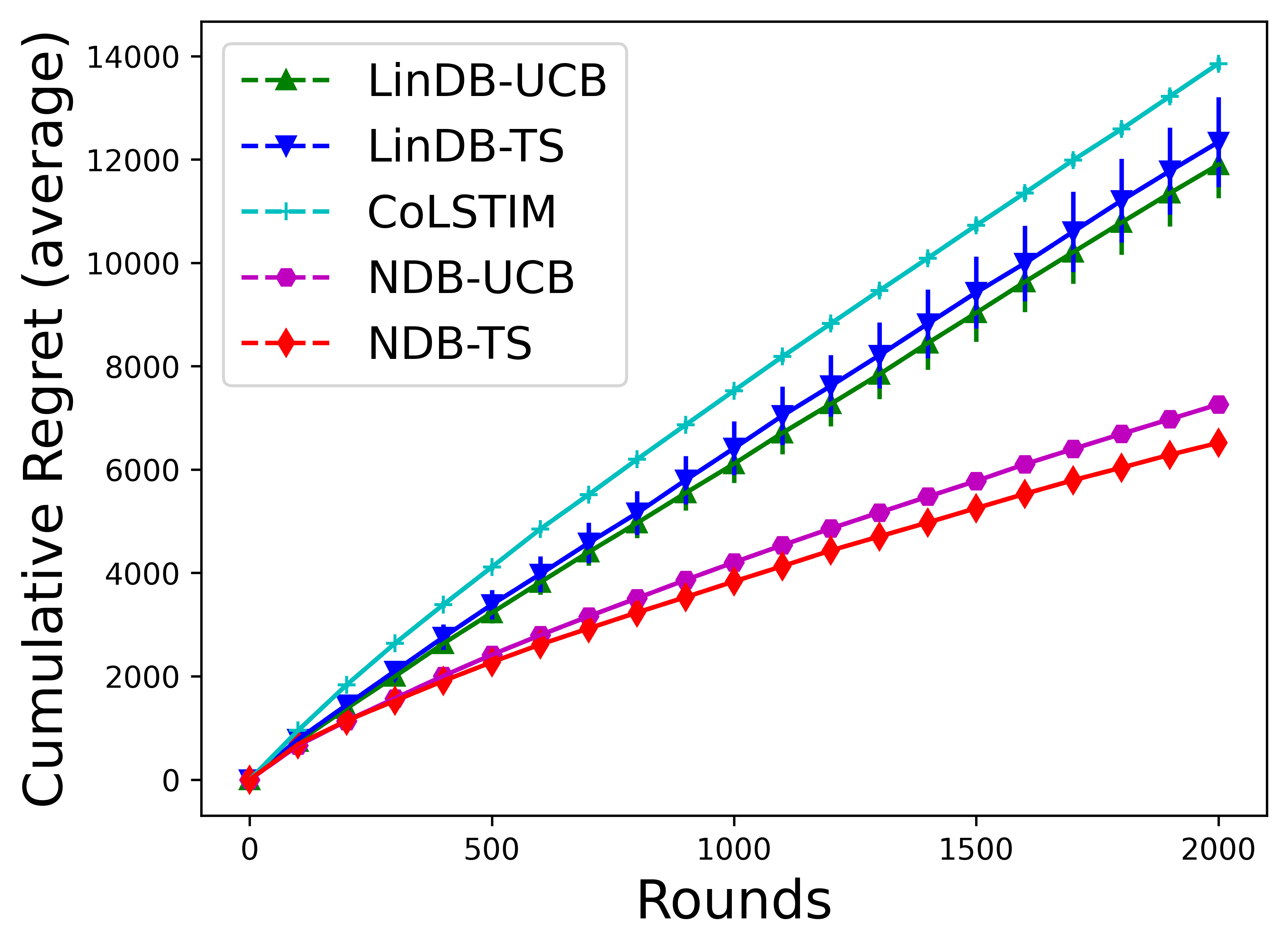
(a) Square (Average)

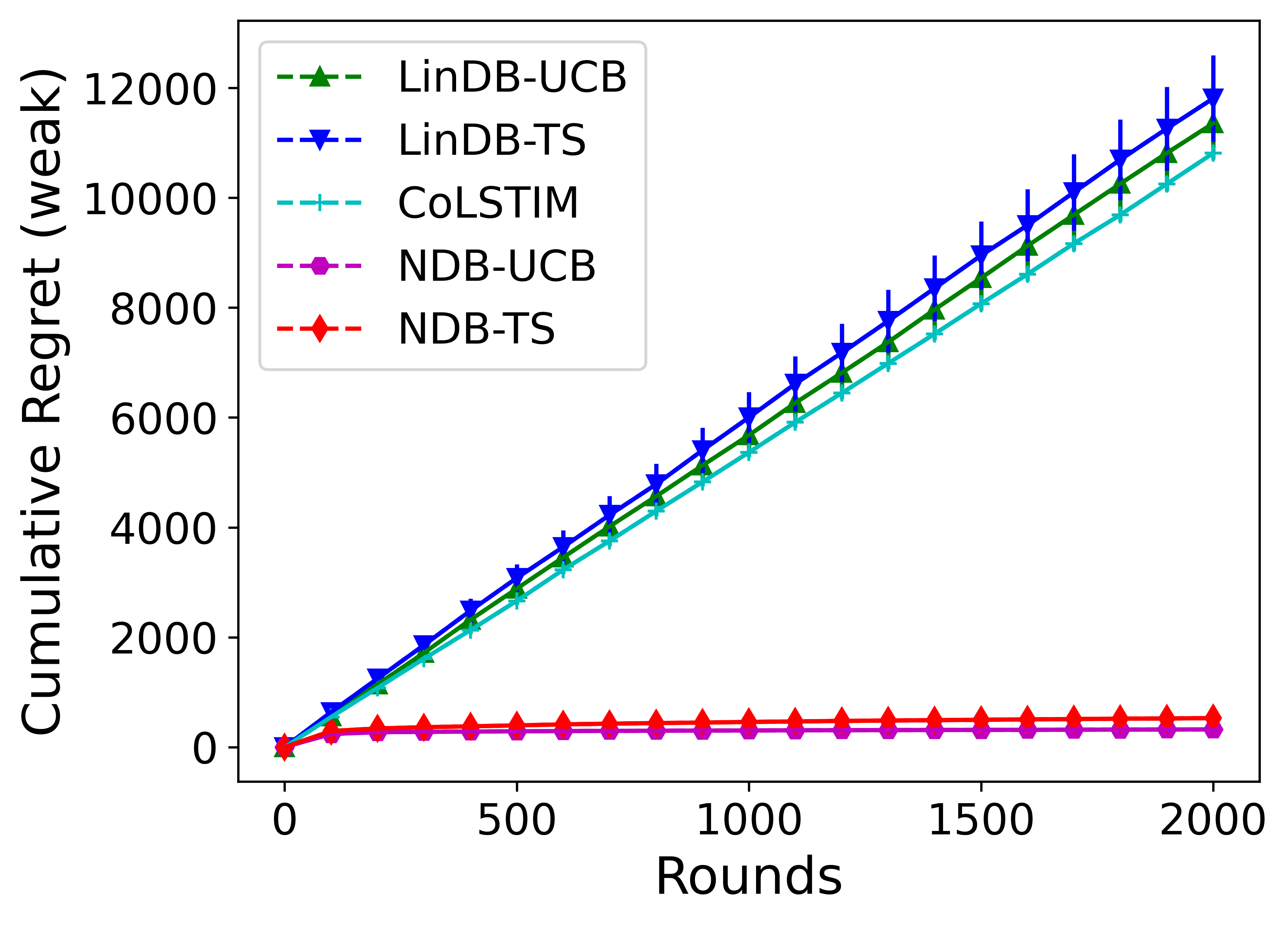
(b) Square (Weak)

(c) Cosine (Average)

(d) Cosine (Weak)

Figure 1: Comparisons of cumulative regret (average and weak) of different dueling bandits algorithms for non-linear reward functions: Square $(10(x^{\top}\theta)^{2})$ and Cosine $(cos(3x^{\top}\theta))$.

Varying dimension and arms vs. regret  Increasing the number of arms ($K$) and the dimension of the context-arm feature vectors $(d)$ makes the problem more difficult. To see how increasing $K$ and $d$ affects the regret of our proposed algorithms, we vary the $K=\{5,10,15,20,25\}$ and $d=\{5,10,15,20,25\}$ while keeping the other problem parameters constant. As expected, the regret of NDB-UCB increases with increase in $K$ and $d$ as shown in Fig. 2. We also observe the same behavior for NDB-TS as shown Fig. 4. All missing figures from this section are in the Appendix D.

(a) Varying $K$ (Average)

(b) Varying $K$ (Weak)

(c) Varying $d$ (Average)

(d) Varying $d$ (Weak)

Figure 2: Cumulative regret (average and weak) of NDB-UCB vs. different number of arms $(K)$ and dimension of the context-arm feature vector $(d)$ for Square reward function $(i.e.,10(x^{\top}\theta)^{2})$.

7 Conclusion

Due to their prevalence in many real-life applications, from online recommendations to ranking web search results, we consider contextual dueling bandit problems that can have a complex and non-linear reward function. We used a neural network to estimate this reward function using preference feedback observed for the previously selected arms. We proposed upper confidence bound- and Thompson sampling-based algorithms with sub-linear regret guarantees for contextual dueling bandits. Experimental results using synthetic functions corroborate our theoretical results. Our algorithms and theoretical results can also provide insights into the celebrated reinforcement learning with human feedback (RLHF) algorithm, such as a theoretical guarantee on the quality of the learned reward model. We also extend our results to contextual bandit problems with binary feedback, which is in itself a non-trivial contribution. A limitation of our work is that we currently do not account for problems where multiple arms are selected simultaneously (multi-way preference), which is an interesting future direction. Another future topic is to apply our algorithms to important real-world problems involving preference or binary feedback, e.g., LLM alignment using human feedback.

Appendix A Theoretical Analysis for NDB-UCB

Here, we first list the specific conditions we need for the width $m$ of the NN:

$$\begin{split}&m\geq CT^{4}K^{4}L^{6}\log(T^{2}K^{2}L/\delta)/\lambda_{0}^{4},\\ &m(\log m)^{-3}\geq C\kappa_{\mu}^{-3}T^{8}L^{21}\lambda^{-5},\\ &m(\log m)^{-3}\geq C\kappa_{\mu}^{-3}T^{14}L^{21}\lambda^{-11}L_{\mu}^{6},\\ &m(\log m)^{-3}\geq CT^{14}L^{18}\lambda^{-8},\end{split}$$ (10)

for some absolute constant $C>0$. To ease exposition, we express these conditions above as $m\geq\text{poly}(T,L,K,1/\kappa_{\mu},L_{\mu},1/\lambda_{0},1/\lambda,\log(1/\delta))$.

To simplify exposition, we use an error probability of $\delta$ for all probabilistic statements. Our final results hold naturally by taking a union bound over all required $\delta$’s. The lemma below shows that the ground-truth utility function $f$ can be expressed as a linear function.

Lemma 1 (Lemma B.3 of [8]).

As long as the width $m$ of the NN is wide enough:

$$m\geq C_{0}T^{4}K^{4}L^{6}\log(T^{2}K^{2}L/\delta)/\lambda_{0}^{4},$$

then with probability of at least $1-\delta$, there exits a $\theta_{f}$ such that

$$f(x)=\langle g(x;\theta_{0}),\theta_{f}-\theta_{0}\rangle,\sqrt{m}\left\|\theta_{f}-\theta_{0}\right\|_{2}\leq\sqrt{2\mathbf{h}^{\top}\mathbf{H}^{-1}\mathbf{h}}\leq B.$$

for all $x\in\mathcal{X}_{t},\forall t\in[T]$.

Let $y_{s}=\mathbbm{1}(x_{s,1}\succ x_{s,2})$, then we can write $\mathbb{P}\left(y_{s}=1\right)=\mu\left(h(x_{s,1};\theta)-h(x_{s,2};\theta)\right)$ and $\mathbb{P}\left(y_{s}=0\right)=1-\mu\left(h(x_{s,1};\theta)-h(x_{s,2};\theta)\right)=\mu\left(h(x_{s,2};\theta)-h(x_{s,1};\theta)\right)$.

A.1 Theoretical Guarantee about the Neural Network

The following lemma gives an upper bound on the distance between $\theta_{t}$ and $\theta_{0}$:

Lemma 2.

We have that $\left\|\theta_{t}-\theta_{0}\right\|_{2}\leq 2\sqrt{\frac{t}{m\lambda}},\forall t\in[T]$.

Proof.

As $\mu(\cdot)\in[0,1]$, then using Eq. 1 gives us

$$\frac{1}{2}\lambda\left\|\theta_{t}-\theta_{0}\right\|^{2}_{2} \leq\mathcal{L}_{t}(\theta_{t})\leq\mathcal{L}_{t}(\theta_{0})$$

$$=-\frac{1}{m}\sum^{t-1}_{s=1}\Big{[}\mathbbm{1}_{x_{t,1}\succ x_{t,2}}\log\mu\left(h(x_{s,1};\theta_{0})-h(x_{s,2};\theta_{0})\right)+$$

$$\qquad(1-\mathbbm{1}_{x_{t,1}\succ x_{t,2}})\log\mu\left(h(x_{s,2};\theta_{0})-h(x_{s,1};\theta_{0})\right)\Big{]}+\frac{1}{2}\lambda\left\|\theta_{0}-\theta_{0}\right\|^{2}_{2}$$

$$\stackrel{{\scriptstyle(a)}}{{=}}-\frac{1}{m}\sum^{t-1}_{s=1}\Big{[}\mathbbm{1}_{x_{t,1}\succ x_{t,2}}\log\mu\left(0\right)+(1-\mathbbm{1}_{x_{t,1}\succ x_{t,2}})\log\mu\left(0\right)\Big{]}$$

$$=-\frac{1}{m}\sum^{t-1}_{s=1}\log 0.5$$

$$\leq\frac{1}{m}t(-\log 0.5)$$

$$\stackrel{{\scriptstyle(b)}}{{\leq}}\frac{t}{m}.$$

Step $(a)$ follow because $h(x;\theta_{0})=0,\forall x\in\mathcal{X},t\in[T]$ which is ensured by 2, step $(b)$ follows because $-\log 0.5<1$. Therefore, we have that $\left\|\theta_{t}-\theta_{0}\right\|_{2}\leq\sqrt{2\frac{t}{m\lambda}}\leq 2\sqrt{\frac{t}{m\lambda}}$. ∎

Now, 2 allows us to obtain the following lemmas regarding the gradients of the NN.

Lemma 3.

Let $\tau=2\sqrt{\frac{t}{m\lambda}}$. Then for absolute constants $C_{3},C_{1}>0$, with probability of at least $1-\delta$,

$$\left\|g(x;\theta_{t})\right\|_{2}\leq C_{3}\sqrt{mL},$$

$$\left\|g(x;\theta_{0})-g(x;\theta_{t})\right\|_{2}\leq C_{1}\sqrt{m\log m}\tau^{1/3}L^{7/2}=C_{1}m^{1/3}\sqrt{\log m}\left(\frac{t}{\lambda}\right)^{1/3}L^{7/2},$$

for all $x\in\mathcal{X}_{t},t\in[T]$.

Proof.

It can be easily verified that our $\tau=2\sqrt{\frac{t}{m\lambda}}$ satisfies the requirement on $\tau$ specified in Lemmas B.5 and B.6 from [8]. Therefore, the results from Lemmas B.5 and B.6 from [8] are applicable for $\theta_{t}$ because our 2 guarantees that $\left\|\theta_{t}-\theta_{0}\right\|_{2}\leq\tau$. ∎

In addition, Lemmas B.4 from [7] allows us to obtain the following lemma, which shows that the output of the NN can be approximated by its linearization.

Lemma 4.

Let $\tau\triangleq 2\sqrt{\frac{t}{m\lambda}}$. Let $\varepsilon^{\prime}_{m,t}\triangleq C_{2}m^{-1/6}\sqrt{\log m}L^{3}\left(\frac{t}{\lambda}\right)^{4/3}$. Then for some absolute constant $C_{2}>0$, with probability of at least $1-\delta$,

$$|h(x;\theta_{t})-\langle\theta_{t}-\theta_{0},g(x;\theta_{0})\rangle|\leq C_{2}\tau^{4/3}L^{3}\sqrt{m\log m} =C_{2}m^{-1/6}\sqrt{\log m}L^{3}\left(\frac{t}{\lambda}\right)^{4/3}$$

$$=\varepsilon^{\prime}_{m,t},$$

for all $x\in\mathcal{X}_{t},t\in[T]$.

An immediate consequence of 4 is the following lemma.

Lemma 5.

For all $t\in[T]$, we have for all $x,x^{\prime}\in\mathcal{X}_{t}$ that

$$|\langle\varphi(x)-\varphi(x^{\prime}),\theta_{t}-\theta_{0}\rangle-(h(x;\theta_{t})-h(x^{\prime};\theta_{t}))|\leq 2\varepsilon^{\prime}_{m,t}.$$

Proof.

By re-arranging the left-hand side and then using 4, we get

$$\begin{split}|\langle\varphi(x)&-\varphi(x^{\prime}),\theta_{t}-\theta_{0}\rangle-(h(x;\theta_{t})-h(x^{\prime};\theta_{t}))|\\ &=|\langle\varphi(x),\theta_{t}-\theta_{0}\rangle-h(x;\theta_{t})+h(x^{\prime};\theta_{t})-\langle\varphi(x^{\prime}),\theta_{t}-\theta_{0}\rangle|\\ &\leq|\langle\varphi(x),\theta_{t}-\theta_{0}\rangle-h(x;\theta_{t})|+|h(x^{\prime};\theta_{t})-\langle\varphi(x^{\prime}),\theta_{t}-\theta_{0}\rangle|\\ &\leq 2C_{2}m^{-1/6}\sqrt{\log m}L^{3}\left(\frac{t}{\lambda}\right)^{4/3}\\ &=2\varepsilon^{\prime}_{m,t}.\qed\end{split}$$ (11)

A.2 Proof of Confidence Ellipsoid

In our next proofs, we denote $\varphi^{\prime}_{s}\triangleq g(x_{s,1};\theta_{0})-g(x_{s,2};\theta_{0})$, $\widetilde{\varphi}^{\prime}_{s}\triangleq g(x_{s,1};\theta_{t})-g(x_{s,2};\theta_{t})$, and $\widetilde{h}_{s,t}\triangleq h(x_{s,1};\theta_{t})-h(x_{s,2};\theta_{t})$. Recall that $p$ is the total number of parameters of the NN. We next prove the confidence ellipsoid for our algorithm, including 6 and 1 below.

Lemma 6.

Let $\beta_{T}\triangleq\frac{1}{\kappa_{\mu}}\sqrt{\widetilde{d}+2\log(1/\delta)}$. Assuming that the conditions on $m$ from Eq. 10 are satisfied. With probability of at least $1-\delta$, we have that

$$\sqrt{m}\left\|\theta_{f}-\theta_{t}\right\|_{V_{t-1}}\leq\beta_{T}+B\sqrt{\frac{\lambda}{\kappa_{\mu}}}+1,\qquad\forall t\in[T].$$

A.2.1 Proof of 6

For any $\theta_{f^{\prime}}\in\mathbb{R}^{p}$, define

$$G_{t}(\theta_{f^{\prime}})\triangleq\frac{1}{m}\sum_{s=1}^{t-1}\Big{[}\mu\left(\langle\theta_{f^{\prime}}-\theta_{0},\varphi^{\prime}_{s}\rangle\right)-\mu\left(\langle\theta_{f}-\theta_{0},\varphi^{\prime}_{s}\rangle\right)\Big{]}\varphi^{\prime}_{s}+\lambda(\theta_{f^{\prime}}-\theta_{0}).$$ (12)

We start by decomposing $\left\|\theta_{f}-\theta_{t}\right\|_{V_{t-1}}$ in terms of $G_{t}$ in the following lemma.

Lemma 7.

Choose $\lambda>0$ such that $\lambda/\kappa_{\mu}>1$. Define $V_{t-1}\triangleq\sum_{s=1}^{t-1}\varphi^{\prime}_{s}{\varphi^{\prime}}_{s}^{\top}\frac{1}{m}+\frac{\lambda}{\kappa_{\mu}}\mathbf{I}$.

$$\left\|\theta_{f}-\theta_{t}\right\|_{V_{t-1}}\leq\frac{1}{\kappa_{\mu}}\left\|G_{t}(\theta_{t})\right\|_{V_{t-1}^{-1}}+\sqrt{\frac{\lambda}{\kappa_{\mu}}}\frac{B}{\sqrt{m}}.$$

Proof.

Let $\lambda^{\prime}\in(0,1)$. For any $\theta_{f^{\prime}_{1}},\theta_{f^{\prime}_{2}}\in\mathbb{R}^{p}$, setting $\theta_{\bar{f}}=\lambda^{\prime}\theta_{f^{\prime}_{1}}+(1-\lambda^{\prime})\theta_{f^{\prime}_{2}}$ and using mean-value theorem, we get:

$$G_{t}(\theta_{f^{\prime}_{1}})-G_{t}(\theta_{f^{\prime}_{2}}) =\left[\sum_{s=1}^{t-1}\frac{1}{m}\dot{\mu}(\langle\theta_{\bar{f}}-\theta_{0},\varphi^{\prime}_{s}\rangle)\varphi^{\prime}_{s}{\varphi^{\prime}}_{s}^{\top}+\lambda\mathbf{I}_{p}\right](\theta_{f^{\prime}_{1}}-\theta_{f^{\prime}_{2}})$$

$$\geq\kappa_{\mu}\left[\sum_{s=1}^{t-1}\varphi^{\prime}_{s}{\varphi^{\prime}}_{s}^{\top}\frac{1}{m}+\frac{\lambda}{\kappa_{\mu}}\mathbf{I}_{p}\right](\theta_{f^{\prime}_{1}}-\theta_{f^{\prime}_{2}})$$

$$=\kappa_{\mu}V_{t-1}(\theta_{f^{\prime}_{1}}-\theta_{f^{\prime}_{2}}).$$

Note that $G_{t}(\theta_{f})=\lambda(\theta_{f}-\theta_{0})$. Let $f_{t}$ be the estimate of $f$ at the beginning of the iteration $t$ and $f_{t,s}=\langle\theta_{t}-\theta_{0},\varphi^{\prime}_{s}\rangle$. Now using the equation above,

$$\left\|G_{t}(\theta_{t})-\lambda(\theta_{f}-\theta_{0})\right\|_{V_{t-1}^{-1}}^{2} =\left\|G_{t}(\theta_{f})-G_{t}(\theta_{t})\right\|_{V_{t-1}^{-1}}^{2}$$

$$\geq(\kappa_{\mu}V_{t-1}(\theta_{f}-\theta_{t}))^{\top}V_{t-1}^{-1}\kappa_{\mu}V_{t-1}(\theta_{f}-\theta_{t})$$

$$=\kappa_{\mu}^{2}(\theta_{f}-\theta_{t})^{\top}V_{t-1}V_{t-1}^{-1}V_{t-1}(\theta_{f}-\theta_{t})$$

$$=\kappa_{\mu}^{2}\left\|\theta_{f}-\theta_{t}\right\|^{2}_{V_{t-1}}.$$

This allows us to show that

$$\left\|\theta_{f}-\theta_{t}\right\|_{V_{t-1}} \leq\frac{1}{\kappa_{\mu}}\left\|G_{t}(\theta_{t})-\lambda(\theta_{f}-\theta_{0})\right\|_{V_{t-1}^{-1}}\leq\frac{1}{\kappa_{\mu}}\left\|G_{t}(\theta_{t})\right\|_{V_{t-1}^{-1}}+\frac{1}{\kappa_{\mu}}\left\|\lambda(\theta_{f}-\theta_{0})\right\|_{V_{t-1}^{-1}},$$ (13)

in which we have made use of the triangle inequality.

Note that we choose $\lambda$ such that $\frac{\lambda}{\kappa_{\mu}}>1$. This allows us to show that $V_{t-1}\succeq\frac{\lambda}{\kappa_{\mu}}I$ and hence $V_{t-1}^{-1}\preceq\frac{\kappa_{\mu}}{\lambda}I$. Recall that 1 tells us that $\left\|\theta_{f}-\theta_{0}\right\|_{2}\leq\frac{B}{\sqrt{m}}$, which tells us that

$$\begin{split}\frac{1}{\kappa_{\mu}}\left\|\lambda(\theta_{f}-\theta_{0})\right\|_{V_{t-1}^{-1}}&=\frac{\lambda}{\kappa_{\mu}}\sqrt{(\theta_{f}-\theta_{0})^{\top}V_{t-1}^{-1}(\theta_{f}-\theta_{0})}\\ &\leq\frac{\lambda}{\kappa_{\mu}}\sqrt{(\theta_{f}-\theta_{0})^{\top}\frac{\kappa_{\mu}}{\lambda}(\theta_{f}-\theta_{0})}\\ &\leq\sqrt{\frac{\lambda}{\kappa_{\mu}}}\left\|\theta_{f}-\theta_{0}\right\|_{2}\\ &\leq\sqrt{\frac{\lambda}{\kappa_{\mu}}}\frac{B}{\sqrt{m}}.\end{split}$$ (14)

Plugging Eq. 14 into Eq. 13 completes the proof. ∎

Recall that we denote $y_{s}=\mu(f(x_{s,1})-f(x_{s,2}))+\varepsilon_{s}$, in which $y_{s}$ is a binary observation and $\varepsilon_{s}$ can be seen as the observation noise. Next, we derive an upper bound on the first term from 7:

$$\begin{split}\frac{1}{\kappa_{\mu}}\left\|G_{t}(\theta_{t})\right\|_{V_{t-1}^{-1}}&=\frac{1}{\kappa_{\mu}}\left\|\frac{1}{m}\sum_{s=1}^{t-1}\Big{[}\mu(\langle\theta_{t}-\theta_{0},\varphi^{\prime}_{s}\rangle)-\mu(\langle\theta_{f}-\theta_{0},\varphi^{\prime}_{s}\rangle)\Big{]}\varphi^{\prime}_{s}+\lambda(\theta_{t}-\theta_{0})\right\|_{V_{t-1}^{-1}}\\ &=\frac{1}{\kappa_{\mu}}\left\|\frac{1}{m}\sum_{s=1}^{t-1}(\mu(f_{t,s})-\mu\left(f(x_{s,1})-f(x_{s,2})\right))\varphi^{\prime}_{s}+\lambda(\theta_{t}-\theta_{0})\right\|_{V_{t-1}^{-1}}\\ &=\frac{1}{\kappa_{\mu}}\left\|\frac{1}{m}\sum_{s=1}^{t-1}\left(\mu(f_{t,s})-(y_{s}-\varepsilon_{s})\right)\varphi^{\prime}_{s}+\lambda(\theta_{t}-\theta_{0})\right\|_{V_{t-1}^{-1}}\\ &=\frac{1}{\kappa_{\mu}}\left\|\frac{1}{m}\sum_{s=1}^{t-1}(\mu(f_{t,s})-y_{s})\varphi^{\prime}_{s}+\frac{1}{m}\sum_{s=1}^{t-1}\varepsilon_{s}\varphi^{\prime}_{s}+\lambda(\theta_{t}-\theta_{0})\right\|_{V_{t-1}^{-1}}\\ &\leq\frac{1}{\kappa_{\mu}}\left\|\frac{1}{m}\sum_{s=1}^{t-1}(\mu(f_{t,s})-y_{s})\varphi^{\prime}_{s}+\lambda(\theta_{t}-\theta_{0})\right\|_{V_{t-1}^{-1}}+\frac{1}{\kappa_{\mu}}\left\|\frac{1}{m}\sum_{s=1}^{t-1}\varepsilon_{s}\varphi^{\prime}_{s}\right\|_{V_{t-1}^{-1}}.\end{split}$$ (15)

Next, we derive an upper bound on the first term in Eq. 15. To simplify exposition, we define

$$A_{1}\triangleq\frac{1}{m}\sum_{s=1}^{t-1}\Big{(}\mu(f_{t,s})-y_{s}\Big{)}\Big{(}\varphi^{\prime}_{s}-\widetilde{\varphi}^{\prime}_{s}\Big{)},\qquad A_{2}\triangleq\frac{1}{m}\sum_{s=1}^{t-1}\Big{(}\mu(f_{t,s})-\mu(\widetilde{h}_{s,t})\Big{)}\widetilde{\varphi}^{\prime}_{s}.$$ (16)

Now the first term in Eq. 15 can be decomposed as:

$$\begin{split}\Big{|}\Big{|}\frac{1}{m}&\sum_{s=1}^{t-1}\Big{(}\mu(f_{t,s})-y_{s}\Big{)}\varphi^{\prime}_{s}+\lambda(\theta_{t}-\theta_{0})\Big{|}\Big{|}_{V_{t-1}^{-1}}\\ &=\Big{|}\Big{|}\frac{1}{m}\sum_{s=1}^{t-1}\Big{(}\mu(f_{t,s})-y_{s}\Big{)}\Big{(}\varphi^{\prime}_{s}+\widetilde{\varphi}^{\prime}_{s}-\widetilde{\varphi}^{\prime}_{s}\Big{)}+\lambda(\theta_{t}-\theta_{0})\Big{|}\Big{|}_{V_{t-1}^{-1}}\\ &=\Big{|}\Big{|}\frac{1}{m}\sum_{s=1}^{t-1}\Big{(}\mu(f_{t,s})-y_{s}\Big{)}\widetilde{\varphi}^{\prime}_{s}+\lambda(\theta_{t}-\theta_{0})+A_{1}\Big{|}\Big{|}_{V_{t-1}^{-1}}\\ &=\Big{|}\Big{|}\frac{1}{m}\sum_{s=1}^{t-1}\Big{(}\mu(f_{t,s})+\mu(\widetilde{h}_{s,t})-\mu(\widetilde{h}_{s,t})-y_{s}\Big{)}\widetilde{\varphi}^{\prime}_{s}+\lambda(\theta_{t}-\theta_{0})+A_{1}\Big{|}\Big{|}_{V_{t-1}^{-1}}\\ &=\Big{|}\Big{|}\frac{1}{m}\sum_{s=1}^{t-1}\Big{(}\mu(\widetilde{h}_{s,t})-y_{s}\Big{)}\widetilde{\varphi}^{\prime}_{s}+\lambda(\theta_{t}-\theta_{0})+A_{2}+A_{1}\Big{|}\Big{|}_{V_{t-1}^{-1}}\\ &\stackrel{{\scriptstyle(a)}}{{=}}\Big{|}\Big{|}A_{2}+A_{1}\Big{|}\Big{|}_{V_{t-1}^{-1}}\\ &\leq\left\|A_{2}\right\|_{V_{t-1}^{-1}}+\left\|A_{1}\right\|_{V_{t-1}^{-1}}\\ &\leq\sqrt{\frac{\kappa_{\mu}}{\lambda}}\left\|A_{2}\right\|_{2}+\sqrt{\frac{\kappa_{\mu}}{\lambda}}\left\|A_{1}\right\|_{2}.\end{split}$$ (17)

Note that step $(a)$ above follows because

$$\begin{split}\frac{1}{m}\sum_{s=1}^{t-1}&\Big{(}\mu(\widetilde{h}_{s,t})-y_{s}\Big{)}\widetilde{\varphi}^{\prime}_{s}+\lambda(\theta_{t}-\theta_{0})\\ &\qquad=\frac{1}{m}\sum_{s=1}^{t-1}\Big{(}\mu(h(x_{s,1};\theta_{t})-h(x_{s,2};\theta_{t}))-y_{s}\Big{)}(g(x_{s,1};\theta_{t})-g(x_{s,2};\theta_{t}))+\lambda(\theta_{t}-\theta_{0})\\ &\qquad=0,\end{split}$$ (18)

which is ensured by the way in which we train our NN (see Eq. 5). Next, we derive an upper bound on the norm of $A_{1}$. To begin with, we have that

$$\left\|\varphi^{\prime}_{s}-\widetilde{\varphi}^{\prime}_{s}\right\|_{2} =\left\|g(x_{s,1};\theta_{0})-g(x_{s,2};\theta_{0})-g(x_{s,1};\theta_{t})+g(x_{s,2};\theta_{t})\right\|_{2}$$

$$\leq\left\|g(x_{s,1};\theta_{0})-g(x_{s,1};\theta_{t})\right\|_{2}+\left\|g(x_{s,2};\theta_{0})-g(x_{s,2};\theta_{t})\right\|_{2}$$

$$\leq 2C_{1}m^{1/3}\sqrt{\log m}\left(\frac{Ct}{\lambda}\right)^{1/3}L^{7/2},$$

in which the last inequality follows from 3. Now the norm of $A_{1}$ can be bounded as:

$$\begin{split}\left\|A_{1}\right\|_{2}&=\left\|\frac{1}{m}\sum_{s=1}^{t-1}\Big{(}\mu(f_{t,s})-y_{s}\Big{)}\Big{(}\varphi^{\prime}_{s}-\widetilde{\varphi}^{\prime}_{s}\Big{)}\right\|_{2}\\ &\leq\frac{1}{m}\sum_{s=1}^{t-1}\left\|\Big{(}\mu(f_{t,s})-y_{s}\Big{)}\Big{(}\varphi^{\prime}_{s}-\widetilde{\varphi}^{\prime}_{s}\Big{)}\right\|_{2}\\ &=\frac{1}{m}\sum_{s=1}^{t-1}|\mu(f_{t,s})-y_{s}|\left\|\varphi^{\prime}_{s}-\widetilde{\varphi}^{\prime}_{s}\right\|_{2}\\ &\leq\frac{1}{m}\sum_{s=1}^{t-1}\left\|\varphi^{\prime}_{s}-\widetilde{\varphi}^{\prime}_{s}\right\|_{2}\\ &\leq\frac{1}{m}\sum_{s=1}^{t-1}2C_{1}m^{1/3}\sqrt{\log m}\left(\frac{t}{\lambda}\right)^{1/3}L^{7/2}\\ &=m^{-2/3}\sqrt{\log m}t^{4/3}2C_{1}\lambda^{-1/3}L^{7/2}.\end{split}$$ (19)

Next, we proceed to bound the norm of $A_{2}$. Let $\lambda^{\prime}\in(0,1)$, and let $a_{t,s}=\lambda^{\prime}f_{t,s}+(1-\lambda^{\prime})\widetilde{h}_{s,t}$. Following the mean-value theorem, we have for some $\lambda^{\prime}$ that

$$\mu(f_{t,s})-\mu(\widetilde{h}_{s,t})=(f_{t,s}-\widetilde{h}_{s,t})\dot{\mu}(a_{t,s}).$$

Note that $\dot{\mu}(a_{t,s})\leq L_{\mu}$ which follows from our 1. This allows us to show that

$$|\mu(f_{t,s}) -\mu(\widetilde{h}_{s,t})|=|(f_{t,s}-\widetilde{h}_{s,t})\dot{\mu}(a_{t,s})|$$

$$=|f_{t,s}-\widetilde{h}_{s,t}||\dot{\mu}(a_{t,s})|$$

$$\leq L_{\mu}|f_{t,s}-\widetilde{h}_{s,t}|$$

$$=L_{\mu}\big{|}\langle\theta_{t}-\theta_{0},g(x_{s,1};\theta_{0})\rangle-\langle\theta_{t}-\theta_{0},g(x_{s,2};\theta_{0})\rangle-(h(x_{s,1};\theta_{t})-h(x_{s,2};\theta_{t}))\big{|}$$

$$\leq L_{\mu}\left(\big{|}\langle\theta_{t}-\theta_{0},g(x_{s,1};\theta_{0})\rangle-h(x_{s,1};\theta_{t})\big{|}+\big{|}h(x_{s,2};\theta_{t})-\langle\theta_{t}-\theta_{0},g(x_{s,2};\theta_{0})\rangle\big{|}\right)$$

$$\leq L_{\mu}\times 2\times C_{2}m^{-1/6}\sqrt{\log m}L^{3}\left(\frac{t}{\lambda}\right)^{4/3}$$

$$=2L_{\mu}C_{2}m^{-1/6}\sqrt{\log m}L^{3}\left(\frac{t}{\lambda}\right)^{4/3}$$

in which we have used 4 in the last inequality. Also, 3 allows us to show that $\left\|\widetilde{\varphi}^{\prime}_{s}\right\|_{2}=\left\|g(x_{s,1};\theta_{t})-g(x_{s,2};\theta_{t})\right\|_{2}\leq\left\|g(x_{s,1};\theta_{t})\right\|_{2}+\left\|g(x_{s,2};\theta_{t})\right\|_{2}\leq 2C_{3}\sqrt{mL}$.

Now we can derive an upper bound on the norm of $A_{2}$:

$$\begin{split}\left\|A_{2}\right\|_{2}&=\left\|\frac{1}{m}\sum_{s=1}^{t-1}\Big{(}\mu(f_{t,s})-\mu(\widetilde{h}_{s,t})\Big{)}\widetilde{\varphi}^{\prime}_{s}\right\|_{2}\\ &\leq\frac{1}{m}\sum_{s=1}^{t-1}\left\|\big{(}\mu(f_{t,s})-\mu(\widetilde{h}_{s,t})\big{)}\widetilde{\varphi}^{\prime}_{s}\right\|_{2}\\ &=\frac{1}{m}\sum_{s=1}^{t-1}|\mu(f_{t,s})-\mu(\widetilde{h}_{s,t})|\left\|\widetilde{\varphi}^{\prime}_{s}\right\|_{2}\\ &\leq\frac{1}{m}\sum_{s=1}^{t-1}2L_{\mu}C_{2}m^{-1/6}\sqrt{\log m}L^{3}\left(\frac{t}{\lambda}\right)^{4/3}\times 2C_{3}\sqrt{mL}\\ &\leq 4L_{\mu}C_{2}C_{3}m^{-2/3}\sqrt{\log m}t^{7/3}L^{7/2}\lambda^{-4/3}.\end{split}$$ (20)

Lastly, plugging Eq. 19 and Eq. 20 into Eq. 17, we can derive an upper bound on the first term in Eq. 15:

$$\begin{split}\frac{1}{\kappa_{\mu}}&\left\|\frac{1}{m}\sum_{s=1}^{t-1}(\mu(f_{t,s})-y_{s})\varphi^{\prime}_{s}+\lambda(\theta_{t}-\theta_{0})\right\|_{V_{t-1}^{-1}}\\ &\leq\frac{1}{\sqrt{\kappa_{\mu}\lambda}}m^{-2/3}\sqrt{\log m}t^{4/3}2C_{1}\lambda^{-1/3}L^{7/2}+\\ &\qquad\qquad\qquad\frac{1}{\sqrt{\kappa_{\mu}\lambda}}4L_{\mu}C_{2}C_{3}m^{-2/3}\sqrt{\log m}t^{7/3}L^{7/2}\lambda^{-4/3}.\end{split}$$ (21)

Next, plugging equation Eq. 21 into equation Eq. 15, and plugging the results into 7, we have that

$$\left\|\theta_{f}-\theta_{t}\right\|_{V_{t-1}}$$

$$\qquad\leq\frac{1}{\kappa_{\mu}\sqrt{m}}\left\|\sum_{s=1}^{t-1}\varepsilon_{s}\varphi^{\prime}_{s}\frac{1}{\sqrt{m}}\right\|_{V_{t-1}^{-1}}+\sqrt{\frac{\lambda}{\kappa_{\mu}}}\frac{B}{\sqrt{m}}+\frac{1}{\sqrt{\kappa_{\mu}\lambda}}m^{-2/3}\sqrt{\log m}t^{4/3}2C_{1}\lambda^{-1/3}L^{7/2}+$$

$$\qquad\qquad\qquad\frac{1}{\sqrt{\kappa_{\mu}\lambda}}4L_{\mu}C_{2}C_{3}m^{-2/3}\sqrt{\log m}t^{7/3}L^{7/2}\lambda^{-4/3}.$$

Here we define

$$\begin{split}\varepsilon_{m,t}&\triangleq B\sqrt{\frac{\lambda}{\kappa_{\mu}}}+\frac{1}{\sqrt{\kappa_{\mu}\lambda}}m^{-1/6}\sqrt{\log m}t^{4/3}2C_{1}\lambda^{-1/3}L^{7/2}+\\ &\qquad\frac{1}{\sqrt{\kappa_{\mu}\lambda}}4L_{\mu}C_{2}C_{3}m^{-1/6}\sqrt{\log m}t^{7/3}L^{7/2}\lambda^{-4/3}.\end{split}$$ (22)

It is easy to verify that as long as the conditions on $m$ from Eq. 10 are satisfied (i.e., the width $m$ of the NN is large enough), we have that $\varepsilon_{m,t}\leq B\sqrt{\frac{\lambda}{\kappa_{\mu}}}+1$.

This allows us to show that

$$\begin{split}\sqrt{m}\left\|\theta_{f}-\theta_{t}\right\|_{V_{t-1}}&\leq\frac{1}{\kappa_{\mu}}\left\|\sum_{s=1}^{t-1}\varepsilon_{s}\varphi^{\prime}_{s}\frac{1}{\sqrt{m}}\right\|_{V_{t-1}^{-1}}+\varepsilon_{m,t}\\ &\leq\frac{1}{\kappa_{\mu}}\left\|\sum_{s=1}^{t-1}\varepsilon_{s}\varphi^{\prime}_{s}\frac{1}{\sqrt{m}}\right\|_{V_{t-1}^{-1}}+B\sqrt{\frac{\lambda}{\kappa_{\mu}}}+1.\end{split}$$ (23)

Finally, in the next lemma, we derive an upper bound on the first term in Eq. 23.

Lemma 8.

Let $\beta_{T}\triangleq\frac{1}{\kappa_{\mu}}\sqrt{\widetilde{d}+2\log(1/\delta)}$. With probability of at least $1-\delta$, we have that

$$\frac{1}{\kappa_{\mu}}\left\|\sum_{s=1}^{t-1}\varepsilon_{s}\varphi^{\prime}_{s}\frac{1}{\sqrt{m}}\right\|_{V_{t-1}^{-1}}\leq\beta_{T}.$$

Proof.

To begin with, we derive an upper bound on the log determinant of the matrix $V_{t}\triangleq\sum_{s=1}^{t}\varphi^{\prime}_{s}{\varphi^{\prime}}_{s}^{\top}\frac{1}{m}+\frac{\lambda}{\kappa_{\mu}}\mathbf{I}$. Here we use $C^{K}_{2}$ to denote all possible pairwise combinations of the indices of $K$ arms. Here we denote $z^{i}_{j}(s)\triangleq\varphi(x_{s,i})-\varphi(x_{s,j})$. Also recall we have defined in the main text that $\mathbf{H}^{\prime}\triangleq\sum_{s=1}^{T}\sum_{(i,j)\in C^{K}_{2}}z^{i}_{j}(s)z^{i}_{j}(s)^{\top}\frac{1}{m}$. Now the determinant of $V_{t}$ can be upper-bounded as

$$\begin{split}\det(V_{t})&=\det\left(\sum_{s=1}^{t}\left(\varphi(x_{s,1})-\varphi(x_{s,2})\right)\left(\varphi(x_{s,1})-\varphi(x_{s,2})\right)^{\top}\frac{1}{m}+\frac{\lambda}{\kappa_{\mu}}\mathbf{I}\right)\\ &\leq\det\left(\sum_{s=1}^{T}\left(\varphi(x_{s,1})-\varphi(x_{s,2})\right)\left(\varphi(x_{s,1})-\varphi(x_{s,2})\right)^{\top}\frac{1}{m}+\frac{\lambda}{\kappa_{\mu}}\mathbf{I}\right)\\ &\leq\det\left(\sum_{s=1}^{T}\sum_{(i,j)\in C^{K}_{2}}z^{i}_{j}(s)z^{i}_{j}(s)^{\top}\frac{1}{m}+\frac{\lambda}{\kappa_{\mu}}\mathbf{I}\right)\\ &=\det\left(\mathbf{H}^{\prime}+\frac{\lambda}{\kappa_{\mu}}\mathbf{I}\right).\end{split}$$ (24)

Recall that in our algorithm, we have set $V_{0}=\frac{\lambda}{\kappa_{\mu}}\mathbf{I}_{p}$. This leads to

$$\begin{split}\log\frac{\det V_{t}}{\det V_{0}}&\leq\log\frac{\det\left(\mathbf{H}^{\prime}+\frac{\lambda}{\kappa_{\mu}}\mathbf{I}\right)}{\det V_{0}}\\ &=\log\frac{(\lambda/\kappa_{\mu})^{p}\det\left(\frac{\kappa_{\mu}}{\lambda}\mathbf{H}^{\prime}+\mathbf{I}\right)}{(\lambda/\kappa_{\mu})^{p}}\\ &=\log\det\left(\frac{\kappa_{\mu}}{\lambda}\mathbf{H}^{\prime}+\mathbf{I}\right).\end{split}$$ (25)

We use $\varepsilon_{s}$ to denote the observation noise in iteration $s\in[T]$: $y_{s}=\mu(f(x_{s,1})-f(x_{s,2}))+\varepsilon_{s}$. Let $\mathcal{F}_{t-1}$ denote the sigma algebra generated by history $\{\left(x_{s,1},x_{s,2},\varepsilon_{s}\right)_{s\in[t-1]},x_{t,1},x_{t,2}\}$. Here we justify that the sequence of noise $\{\varepsilon_{s}\}_{s=1,\ldots,T}$ is conditionally $1$-sub-Gaussian conditioned on $\mathcal{F}_{t-1}$.

Note that the observation $y_{t}$ is equal to $1$ if $x_{t,1}$ is preferred over $x_{t,2}$ and $0$ otherwise. Therefore, the noise $\varepsilon_{t}$ can be expressed as

$$\varepsilon_{t}=\begin{cases}1-\mu(f(x_{t,1})-f(x_{t,2})),&\text{w.p. }\mu(f(x_{t,1})-f(x_{t,2}))\\ -\mu(f(x_{t,1})-f(x_{t,2})),&\text{w.p. }1-\mu(f(x_{t,1})-f(x_{t,2})),\end{cases}$$

It can be easily seen that $\varepsilon_{s}$ is $\mathcal{F}_{t}$-measurable. Next, if can be easily verified that that conditioned on $\mathcal{F}_{t-1}$ (i.e., given $x_{t,1}$ and $x_{t,2}$), we have that $\mathbb{E}\left[\varepsilon_{t}|\mathcal{F}_{t-1}\right]=0$. Also note that the absolute value of $\varepsilon_{t}$ is bounded: $|\varepsilon_{t}|\leq 1$. Therefore, we can infer that $\varepsilon_{t}$ is conditionally $1$-sub-Gaussian, i.e.,

$$\mathbb{E}\left[\exp(\lambda\varepsilon_{t})|\mathcal{F}_{t}\right]\leq\exp\left(\frac{\lambda^{2}\sigma^{2}}{2}\right),\hskip 5.69054pt\forall\lambda\in\mathbb{R}.$$

with $\sigma=1$.

Next, making use of the $1$-sub-sub-Gaussianity of the sequence of noise $\{\varepsilon_{s}\}$ and Theorem 1 from [18], we can show that with probability of at least $1-\delta$,

$$\left\|\sum_{s=1}^{t-1}\varepsilon_{s}\varphi^{\prime}_{s}\frac{1}{\sqrt{m}}\right\|_{V_{t-1}^{-1}} \leq\sqrt{\log\left(\frac{\det V_{t-1}}{\det V_{0}}\right)+2\log(1/\delta)}$$

$$\leq\sqrt{\log\det\left(\frac{\kappa_{\mu}}{\lambda}\mathbf{H}^{\prime}+\mathbf{I}\right)+2\log(1/\delta)}$$

$$\leq\sqrt{\widetilde{d}+2\log(1/\delta)},$$

in which we have made use of the definition of the effective dimension $\widetilde{d}=\log\det\left(\frac{\kappa_{\mu}}{\lambda}\mathbf{H}^{\prime}+\mathbf{I}\right)$. This completes the proof. ∎

Finally, we plug 8 into equation Eq. 23 to complete the proof of 6:

$$\sqrt{m}\left\|\theta_{f}-\theta_{t}\right\|_{V_{t-1}}\leq\beta_{T}+B\sqrt{\frac{\lambda}{\kappa_{\mu}}}+1,\qquad\forall t\in[T].$$

A.2.2 Proof of 1

See 1

Proof.

Denote $\varphi(x)=g(x;\theta_{0})$. Recall that 1 tells us that $f(x)=\langle g(x;\theta_{0}),\theta_{f}-\theta_{0}\rangle=\langle\varphi(x),\theta_{f}-\theta_{0}\rangle$ for all $x\in\mathcal{X}_{t},t\in[T]$. To begin with, for all $x,x^{\prime}\in\mathcal{X}_{t},t\in[T]$ we have that

$$\begin{split}|&f(x)-f(x^{\prime})-\langle\varphi(x)-\varphi(x^{\prime}),\theta_{t}-\theta_{0}\rangle|\\ &=|\langle\varphi(x)-\varphi(x^{\prime}),\theta_{f}-\theta_{0}\rangle-\langle\varphi(x)-\varphi(x^{\prime}),\theta_{t}-\theta_{0}\rangle|\\ &=|\langle\varphi(x)-\varphi(x^{\prime}),\theta_{f}-\theta_{t}\rangle\rangle|\\ &=|\langle\frac{1}{\sqrt{m}}\varphi(x)-\varphi(x^{\prime}),\sqrt{m}\left(\theta_{f}-\theta_{t}\right)\rangle|\\ &\leq\left\|\frac{1}{\sqrt{m}}\left(\varphi(x)-\varphi(x^{\prime})\right)\right\|_{V_{t-1}^{-1}}\sqrt{m}\left\|\theta_{f}-\theta_{t}\right\|_{V_{t-1}}\\ &\leq\left\|\frac{1}{\sqrt{m}}\left(\varphi(x)-\varphi(x^{\prime})\right)\right\|_{V_{t-1}^{-1}}\left(\beta_{T}+B\sqrt{\frac{\lambda}{\kappa_{\mu}}}+1\right),\end{split}$$ (26)

in which we have used 6 in the last inequality. Now making use of the equation above and 5, we have that

$$|f(x)-f(x^{\prime}) -(h(x;\theta_{t})-h(x^{\prime};\theta_{t}))|$$

$$=|f(x)-f(x^{\prime})-\langle\varphi(x)-\varphi(x^{\prime}),\theta_{t}-\theta_{0}\rangle$$

$$\qquad\qquad\qquad+\langle\varphi(x)-\varphi(x^{\prime}),\theta_{t}-\theta_{0}\rangle-(h(x;\theta_{t})-h(x^{\prime};\theta_{t}))|$$

$$\leq|(f(x)-f(x^{\prime}))-\langle\varphi(x)-\varphi(x^{\prime}),\theta_{t}-\theta_{0}\rangle|$$

$$\qquad\qquad\qquad+|\langle\varphi(x)-\varphi(x^{\prime}),\theta_{t}-\theta_{0}\rangle-(h(x;\theta_{t})-h(x^{\prime};\theta_{t}))|$$

$$\leq\left\|\frac{1}{\sqrt{m}}\left(\varphi(x)-\varphi(x^{\prime})\right)\right\|_{V_{t-1}^{-1}}\left(\beta_{T}+B\sqrt{\frac{\lambda}{\kappa_{\mu}}}+1\right)+2\varepsilon^{\prime}_{m,t}.$$

This completes the proof of 1. ∎

A.3 Regret Analysis

Now we can analyze the instantaneous regret. To begin with, we have

$$2r_{t} =f(x_{t}^{*})-f(x_{t,1})+f(x_{t}^{*})-f(x_{t,2})$$

$$\stackrel{{\scriptstyle(a)}}{{\leq}}\langle\varphi(x^{*}_{t})-\varphi(x_{t,1}),\theta_{t}-\theta_{0}\rangle+\left\|\frac{1}{\sqrt{m}}\left(\varphi(x^{*}_{t})-\varphi(x_{t,1})\right)\right\|_{V_{t-1}^{-1}}\left(\beta_{T}+B\sqrt{\lambda/\kappa_{\mu}}+1\right)$$

$$\qquad+\langle\varphi(x^{*}_{t})-\varphi(x_{t,2}),\theta_{t}-\theta_{0}\rangle+\left\|\frac{1}{\sqrt{m}}\left(\varphi(x^{*}_{t})-\varphi(x_{t,2})\right)\right\|_{V_{t-1}^{-1}}\left(\beta_{T}+B\sqrt{\lambda/\kappa_{\mu}}+1\right)$$

$$=\langle\varphi(x^{*}_{t})-\varphi(x_{t,1}),\theta_{t}-\theta_{0}\rangle+\left\|\frac{1}{\sqrt{m}}\left(\varphi(x^{*}_{t})-\varphi(x_{t,1})\right)\right\|_{V_{t-1}^{-1}}\left(\beta_{T}+B\sqrt{\lambda/\kappa_{\mu}}+1\right)$$

$$\qquad+\langle\varphi(x^{*}_{t})-\varphi(x_{t,1}),\theta_{t}-\theta_{0}\rangle+\langle\varphi(x_{t,1})-\varphi(x_{t,2}),\theta_{t}-\theta_{0}\rangle$$

$$\qquad+\left\|\frac{1}{\sqrt{m}}\left(\varphi(x^{*}_{t})-\varphi(x_{t,1})+\varphi(x_{t,1})-\varphi(x_{t,2})\right)\right\|_{V_{t-1}^{-1}}\left(\beta_{T}+B\sqrt{\lambda/\kappa_{\mu}}+1\right)$$

$$\leq 2\langle\varphi(x^{*}_{t})-\varphi(x_{t,1}),\theta_{t}-\theta_{0}\rangle+2\left\|\frac{1}{\sqrt{m}}\left(\varphi(x^{*}_{t})-\varphi(x_{t,1})\right)\right\|_{V_{t-1}^{-1}}\left(\beta_{T}+B\sqrt{\lambda/\kappa_{\mu}}+1\right)$$

$$\quad+\langle\varphi(x_{t,1})-\varphi(x_{t,2}),\theta_{t}-\theta_{0}\rangle+\left\|\frac{1}{\sqrt{m}}\left(\varphi(x_{t,1})-\varphi(x_{t,2})\right)\right\|_{V_{t-1}^{-1}}\left(\beta_{T}+B\sqrt{\lambda/\kappa_{\mu}}+1\right)$$

$$\stackrel{{\scriptstyle(b)}}{{\leq}}2h(x^{*}_{t};\theta_{t})-2h(x_{t,1};\theta_{t})+4\varepsilon^{\prime}_{m,t}+2\left\|\frac{1}{\sqrt{m}}\left(\varphi(x^{*}_{t})-\varphi(x_{t,1})\right)\right\|_{V_{t-1}^{-1}}\left(\beta_{T}+B\sqrt{\lambda/\kappa_{\mu}}+1\right)$$

$$\quad+h(x_{t,1};\theta_{t})-h(x_{t,2};\theta_{t})+2\varepsilon^{\prime}_{m,t}+\left\|\frac{1}{\sqrt{m}}\left(\varphi(x_{t,1})-\varphi(x_{t,2})\right)\right\|_{V_{t-1}^{-1}}\left(\beta_{T}+B\sqrt{\lambda/\kappa_{\mu}}+1\right)$$

$$\stackrel{{\scriptstyle(c)}}{{\leq}}2h(x_{t,2};\theta_{t})-2h(x_{t,1};\theta_{t})+2\left\|\frac{1}{\sqrt{m}}\left(\varphi(x_{t,2})-\varphi(x_{t,1})\right)\right\|_{V_{t-1}^{-1}}\left(\beta_{T}+B\sqrt{\lambda/\kappa_{\mu}}+1\right)$$

$$\quad+h(x_{t,1};\theta_{t})-h(x_{t,2};\theta_{t})+6\varepsilon^{\prime}_{m,t}+\left\|\frac{1}{\sqrt{m}}\left(\varphi(x_{t,1})-\varphi(x_{t,2})\right)\right\|_{V_{t-1}^{-1}}\left(\beta_{T}+B\sqrt{\lambda/\kappa_{\mu}}+1\right)$$

$$=h(x_{t,2};\theta_{t})-h(x_{t,1};\theta_{t})+3\left\|\frac{1}{\sqrt{m}}\left(\varphi(x_{t,1})-\varphi(x_{t,2})\right)\right\|_{V_{t-1}^{-1}}\left(\beta_{T}+B\sqrt{\lambda/\kappa_{\mu}}+1\right)+6\varepsilon^{\prime}_{m,t}$$

$$\stackrel{{\scriptstyle(d)}}{{\leq}}3\left(\beta_{T}+B\sqrt{\lambda/\kappa_{\mu}}+1\right)\left\|\frac{1}{\sqrt{m}}\left(\varphi(x_{t,1})-\varphi(x_{t,2})\right)\right\|_{V_{t-1}^{-1}}+6\varepsilon^{\prime}_{m,t}.$$

Step $(a)$ follows from Eq. 26, step $(b)$ results from 5, step $(c)$ follows from the way in which $x_{t,2}$ is selected: $x_{t,2}=\arg\max_{x\in\mathcal{X}_{t}}\left(h(x;\theta_{t})+\left\|\frac{1}{\sqrt{m}}\left(\varphi(x)-\varphi(x_{t,1})\right)\right\|_{V_{t-1}^{-1}}\left(\beta_{T}+B\sqrt{\frac{\lambda}{\kappa_{\mu}}}+1\right)\right)$, and step $(d)$ follows from the way in which $x_{t,1}$ is selected: $x_{t,1}=\arg\max_{x\in\mathcal{X}_{t}}h(x;\theta_{t})$.

Now denote $\sigma_{t-1}^{2}(x_{t,1},x_{t,2})\doteq\frac{\lambda}{\kappa_{\mu}}\left\|\frac{1}{\sqrt{m}}(\varphi(x_{t,1})-\varphi(x_{t,2}))\right\|^{2}_{V_{t-1}^{-1}}$. Of note, $\sigma_{t-1}^{2}(x_{t,1},x_{t,2})$ can be interpreted as the Gaussian process posterior variance with the kernel defined as $k\big{(}(x_{1},x_{2}),(x^{\prime}_{1},x^{\prime}_{2})\big{)}=\langle\frac{1}{\sqrt{m}}\left(\varphi(x_{1})-\varphi(x_{2})\right),(\frac{1}{\sqrt{m}}(\varphi(x^{\prime}_{1})-\varphi(x^{\prime}_{2}))\rangle$, and with a noise variance of $\frac{\lambda}{\kappa_{\mu}}$. It is easy to see that the kernel is positive semi-definite and is hence a valid kernel. Following the derivations of the Gaussian process posterior variance, it is easy to verify that

$$\sigma_{t-1}^{2}(x_{t,1},x_{t,2}) \leq(\varphi(x_{t,1})-\varphi(x_{t,2}))^{\top}(\varphi(x_{t,1})-\varphi(x_{t,2}))\frac{1}{m}$$

$$=\left\|\left(\varphi(x_{t,1})-\varphi(x_{t,2})\right)\frac{1}{\sqrt{m}}\right\|_{2}^{2}$$

$$=\frac{1}{m}\left\|\varphi(x_{t,1})-\varphi(x_{t,2})\right\|_{2}^{2}\leq c_{0},$$

in which we have denoted $c_{0}>0$ as an absolute constant such that $\frac{1}{m}\left\|\varphi(x)-\varphi(x^{\prime})\right\|_{2}^{2}\leq c_{0},\forall x,x^{\prime}\in\mathcal{X}_{t},t\in[T]$. Note that this is similar to the standard assumption in the literature that the value of the NTK is upper-bounded by a constant [47]. Therefore, this implies that $\sigma_{t-1}^{2}(x_{t,1},x_{t,2})/c_{0}\leq 1$ for some constant $c_{0}\geq 1$. Recall that we choose $\lambda$ such that $\lambda/\kappa_{\mu}\geq 1$. Note that for any $\alpha\in[0,1]$, we have that $\alpha/2\leq\log(1+\alpha)$. With these, we have that

$$\frac{1}{2}\left(\frac{\lambda}{\kappa_{\mu}}\right)^{-1}\frac{\sigma_{t-1}^{2}(x_{t,1},x_{t,2})}{c_{0}} \leq\log\left(1+\left(\frac{\lambda}{\kappa_{\mu}}\right)^{-1}\frac{\sigma_{t-1}^{2}(x_{t,1},x_{t,2})}{c_{0}}\right)$$

$$\leq\log\left(1+\left(\frac{\lambda}{\kappa_{\mu}}\right)^{-1}\sigma_{t-1}^{2}(x_{t,1},x_{t,2})\right),$$

which leads to

$$\sigma_{t-1}^{2}(x_{t,1},x_{t,2})\leq 2c_{0}\frac{\lambda}{\kappa_{\mu}}\log\left(1+\frac{\kappa_{\mu}}{\lambda}\sigma_{t-1}^{2}(x_{t,1},x_{t,2})\right).$$ (27)

Following the analysis of [14] and using the chain rule of conditional information gain, we can show that

$$\sum^{t}_{s=1}\log\left(1+\frac{\kappa_{\mu}}{\lambda}\sigma_{s-1}^{2}(x_{s,1},x_{s,2})\right)=\log\det\left(\mathbf{I}+\frac{\kappa_{\mu}}{\lambda}\mathbf{K}_{t}\right),$$

in which $\mathbf{K}_{t}$ is a $t\times t$ matrix in which every element is $\mathbf{K}_{t}[i,j]=\frac{1}{m}(\varphi(x_{i,1})-\varphi(x_{i,2}))^{\top}(\varphi(x_{j,1})-\varphi(x_{j,2}))$. Define the $p\times t$ matrix $\mathbf{J}_{t}=[\frac{1}{\sqrt{m}}\left(\varphi(x_{i,1})-\varphi(x_{i,2})\right)]_{i=1,\ldots,t}$. Then we have that $\mathbf{K}_{t}=\mathbf{J}_{t}^{\top}\mathbf{J}_{t}$. This allows us to show that

$$\begin{split}\sum^{t}_{s=1}&\log\left(1+\frac{\kappa_{\mu}}{\lambda}\sigma_{s-1}^{2}(x_{s,1},x_{s,2})\right)=\log\det\left(\mathbf{I}+\frac{\kappa_{\mu}}{\lambda}\mathbf{K}_{t}\right)\\ &=\log\det\left(\mathbf{I}+\frac{\kappa_{\mu}}{\lambda}\mathbf{J}_{t}^{\top}\mathbf{J}_{t}\right)\\ &=\log\det\left(\mathbf{I}+\frac{\kappa_{\mu}}{\lambda}\mathbf{J}_{t}\mathbf{J}_{t}^{\top}\right)\\ &=\log\det\left(\mathbf{I}+\frac{\kappa_{\mu}}{\lambda}\sum_{s=1}^{t}\left(\varphi(x_{s,1})-\varphi(x_{s,2})\right)\left(\varphi(x_{s,1})-\varphi(x_{s,2})\right)^{\top}\frac{1}{m}\right)\\ &\leq\log\det\left(\frac{\kappa_{\mu}}{\lambda}\mathbf{H}^{\prime}+\mathbf{I}\right)\\ &=\widetilde{d}\end{split}$$ (28)

in which we have followed the same line of analysis as Eq. 24 and Eq. 25 in the second last inequality.

Combining the results from Eq. 27 and Eq. 28, we have that

$$\sum^{T}_{t=1}\sigma_{t-1}^{2}(x_{t,1},x_{t,2}) \leq 2c_{0}\frac{\lambda}{\kappa_{\mu}}\sum^{T}_{t=1}\log\left(1+\frac{\kappa_{\mu}}{\lambda}\sigma_{t-1}^{2}(x_{t,1},x_{t,2})\right)$$

$$\leq 2c_{0}\frac{\lambda}{\kappa_{\mu}}\widetilde{d}.$$

Finally, we can derive an upper bound on the cumulative regret:

$$\mathfrak{R}_{T} =\sum^{T}_{t=1}r_{t}\leq\sum^{T}_{t=1}\frac{1}{2}\left(3\left(\beta_{T}+B\sqrt{\frac{\lambda}{\kappa_{\mu}}}+1\right)\sqrt{\frac{\kappa_{\mu}}{\lambda}}\sigma_{t-1}(x_{t,1},x_{t,2})+6\varepsilon^{\prime}_{m,t}\right)$$

$$\leq\frac{3}{2}\left(\beta_{T}+B\sqrt{\frac{\lambda}{\kappa_{\mu}}}+1\right)\sqrt{\frac{\kappa_{\mu}}{\lambda}}\sum^{T}_{t=1}\sigma_{t-1}(x_{t,1},x_{t,2})+6T\varepsilon^{\prime}_{m,T}$$

$$\leq\frac{3}{2}\left(\beta_{T}+B\sqrt{\frac{\lambda}{\kappa_{\mu}}}+1\right)\sqrt{\frac{\kappa_{\mu}}{\lambda}}\sqrt{T\sum^{T}_{t=1}\sigma^{2}_{t-1}(x_{t,1},x_{t,2})}+6T\varepsilon^{\prime}_{m,T}$$

$$\leq\frac{3}{2}\left(\beta_{T}+B\sqrt{\frac{\lambda}{\kappa_{\mu}}}+1\right)\sqrt{\frac{\kappa_{\mu}}{\lambda}}\sqrt{T2c_{0}\frac{\lambda}{\kappa_{\mu}}\widetilde{d}}+6T\varepsilon^{\prime}_{m,T}.$$

$$\leq\frac{3}{2}\left(\beta_{T}+B\sqrt{\frac{\lambda}{\kappa_{\mu}}}+1\right)\sqrt{T2c_{0}\widetilde{d}}+6T\varepsilon^{\prime}_{m,T}.$$

Recall that $\varepsilon^{\prime}_{m,t}=C_{2}m^{-1/6}\sqrt{\log m}L^{3}\left(\frac{t}{\lambda}\right)^{4/3}$. It can be easily verified that as long as the conditions on $m$ specified in Eq. 10 are satisfied (i.e., as long as the NN is wide enough), we have that $6T\varepsilon^{\prime}_{m,T}\leq 1$. Recall that $\beta_{T}=\widetilde{\mathcal{O}}(\frac{1}{\kappa_{\mu}}\sqrt{\widetilde{d}})$. This allows us to simplify the regret upper bound to be

$$\mathfrak{R}_{T} \leq\frac{3}{2}\left(\beta_{T}+B\sqrt{\frac{\lambda}{\kappa_{\mu}}}+1\right)\sqrt{T2c_{0}\widetilde{d}}+1$$

$$=\widetilde{\mathcal{O}}\left(\left(\frac{\sqrt{\widetilde{d}}}{\kappa_{\mu}}+B\sqrt{\frac{\lambda}{\kappa_{\mu}}}\right)\sqrt{\widetilde{d}T}\right).$$

Appendix B Theoretical Analysis for NDB-TS

Denote $\nu_{T}\triangleq\left(\beta_{T}+B\sqrt{\lambda/\kappa_{\mu}}+1\right)\sqrt{\kappa_{\mu}/\lambda}$, $c_{t}\triangleq\nu_{T}(1+\sqrt{2\log(Kt^{2})})$, and $\sigma_{t-1}^{2}(x_{1},x_{2})\triangleq\frac{\lambda}{\kappa_{\mu}}\left\|\frac{1}{\sqrt{m}}(\varphi(x_{1})-\varphi(x_{2}))\right\|^{2}_{V_{t-1}^{-1}}$. Here we use $\mathcal{F}_{t-1}$ to denote the filtration containing the history of selected inputs and observations up to iteration $t-1$. To use Thompson sampling (TS) to select the second arm $x_{t,2}$, firstly, for each arm $x\in\mathcal{X}_{t}$, we sample a reward value $\widetilde{r}_{t}(x)$ from the normal distribution $\mathcal{N}\left(h(x;\theta_{t})-h(x_{t,1};\theta_{t}),\nu_{T}^{2}\sigma_{t-1}^{2}(x,x_{t,1})\right)$. Then, we choose the second arm as $x_{t,2}={\arg\max}_{x\in\mathcal{X}_{t}}\widetilde{r}_{t}(x)$.

Lemma 9.

Let $\delta\in(0,1)$. Define $E^{f}(t)$ as the following event:

$$|\left[f(x)-f(x_{t,1})\right]-\left[h(x;\theta_{t})-h(x_{t,1};\theta_{t})\right]|\leq\nu_{T}\sigma_{t-1}(x,x_{t,1})+2\varepsilon^{\prime}_{m,t}.$$

According to 1, we have that the event $E^{f}(t)$ holds with probability of at least $1-\delta$.

Lemma 10.

Define $E^{f_{t}}(t)$ as the following event

$$|\widetilde{r}_{t}(x)-\left[h(x;\theta_{t})-h(x_{t,1};\theta_{t})\right]|\leq\nu_{T}\sqrt{2\log(Kt^{2})}\sigma_{t-1}(x,x_{t,1}).$$

We have that $\mathbb{P}\left[E^{f_{t}}(t)|\mathcal{F}_{t-1}\right]\geq 1-1/t^{2}$ for any possible filtration $\mathcal{F}_{t-1}$.

Definition 1.

In iteration $t$, define the set of saturated points as

$$S_{t}=\{x\in\mathcal{X}_{t}:\Delta(x)>c_{t}\sigma_{t-1}(x,x_{t,1})+4\varepsilon^{\prime}_{m,t}\},$$

where $\Delta(x)=f(x^{*}_{t})-f(x)$ and $x^{*}_{t}\in\arg\max_{x\in\mathcal{X}_{t}}f(x)$.

Note that according to this definition, $x^{*}_{t}$ is always unsaturated.

Lemma 11.

For any filtration $\mathcal{F}_{t-1}$, conditioned on the event $E^{f}(t)$, we have that $\forall x\in\mathcal{Q}$,

$$\mathbb{P}\left(\widetilde{r}_{t}(x)+2\varepsilon^{\prime}_{m,t}>f(x)-f(x_{t,1})|\mathcal{F}_{t-1}\right)\geq p,$$

where $p=\frac{1}{4e\sqrt{\pi}}$.

Proof.

Adding and subtracting $\frac{\mu_{t-1}(x)}{\nu_{t}\sigma_{t-1}(x)}$ both sides of $\mathbb{P}\left(f_{t}(x)>\rho_{m}f(x)|\mathcal{F}_{t-1}\right)$, we get

$$\mathbb{P}\left\{\widetilde{r}_{t}(x)+2\varepsilon^{\prime}_{m,t}>f(x)-f(x_{t,1})|\mathcal{F}_{t-1}\right\}$$

$$=\mathbb{P}\left\{\frac{\widetilde{r}_{t}(x)+2\varepsilon^{\prime}_{m,t}-\left[h(x;\theta_{t})-h(x_{t,1};\theta_{t})\right]}{\nu_{T}\sigma_{t-1}(x,x_{t,1})}>\frac{f(x)-f(x_{t,1})-\left[h(x;\theta_{t})-h(x_{t,1};\theta_{t})\right]}{\nu_{T}\sigma_{t-1}(x,x_{t,1})}|\mathcal{F}_{t-1}\right\}$$

$$\geq\mathbb{P}\left\{\frac{\widetilde{r}_{t}(x)+2\varepsilon^{\prime}_{m,t}-\left[h(x;\theta_{t})-h(x_{t,1};\theta_{t})\right]}{\nu_{T}\sigma_{t-1}(x,x_{t,1})}>\frac{|f(x)-f(x_{t,1})-\left[h(x;\theta_{t})-h(x_{t,1};\theta_{t})\right]|}{\nu_{T}\sigma_{t-1}(x,x_{t,1})}|\mathcal{F}_{t-1}\right\}$$

$$\geq\mathbb{P}\left\{\frac{\widetilde{r}_{t}(x)-\left[h(x;\theta_{t})-h(x_{t,1};\theta_{t})\right]}{\nu_{T}\sigma_{t-1}(x,x_{t,1})}>\frac{|f(x)-f(x_{t,1})-\left[h(x;\theta_{t})-h(x_{t,1};\theta_{t})\right]|-2\varepsilon^{\prime}_{m,t}}{\nu_{T}\sigma_{t-1}(x,x_{t,1})}|\mathcal{F}_{t-1}\right\}$$

$$\geq\mathbb{P}\left\{\frac{\widetilde{r}_{t}(x)-\left[h(x;\theta_{t})-h(x_{t,1};\theta_{t})\right]}{\nu_{T}\sigma_{t-1}(x,x_{t,1})}>1|\mathcal{F}_{t-1}\right\}$$

$$\geq\frac{1}{4e\sqrt{\pi}},$$

in which the third inequality makes use of 9 (note that we have conditioned on the event $E^{f}(t)$ here), and the last inequality follows from the Gaussian anti-concentration inequality: $\mathbb{P}(z>a)\geq\exp(-a^{2})/(4\sqrt{\pi}a)$ where $z\sim\mathcal{N}(0,1)$. ∎

The next lemma proves a lower bound on the probability that the selected input $x_{t,2}$ is unsaturated.

Lemma 12.

For any filtration $\mathcal{F}_{t-1}$, conditioned on the event $E^{f}(t)$, we have that,

$$\mathbb{P}\left(x_{t,2}\in\mathcal{X}_{t}\setminus S_{t}|\mathcal{F}_{t-1}\right)\geq p-1/t^{2}.$$

Proof.

To begin with, we have that

$$\mathbb{P}\left(x_{t,2}\in\mathcal{X}_{t}\setminus S_{t}|\mathcal{F}_{t-1}\right)\geq\mathbb{P}\left(\widetilde{r}_{t}(x^{*}_{t})>\widetilde{r}_{t}(x),\forall x\in S_{t}|\mathcal{F}_{t-1}\right).$$ (29)

This inequality can be justified because the event on the right hand side implies the event on the left hand side. Specifically, according to 1, $x^{*}_{t}$ is always unsaturated. Therefore, because $x_{t,2}$ is selected by $x_{t,2}={\arg\max}_{x\in\mathcal{X}_{t}}\widetilde{r}_{t}(x)$, we have that if $\widetilde{r}_{t}(x^{*}_{t})>\widetilde{r}_{t}(x),\forall x\in S_{t}$, then the selected $x_{t,2}$ is guaranteed to be unsaturated. Now conditioning on both events $E^{f}(t)$ and $E^{f_{t}}(t)$, for all $x\in S_{t}$, we have that

$$\begin{split}\widetilde{r}_{t}(x)&\leq f(x)-f(x_{t,1})+c_{t}\sigma_{t-1}(x,x_{t,1})+2\varepsilon^{\prime}_{m,t}\\ &=f(x)-f(x_{t,1})+c_{t}\sigma_{t-1}(x,x_{t,1})+4\varepsilon^{\prime}_{m,t}-2\varepsilon^{\prime}_{m,t}\\ &\leq f(x)-f(x_{t,1})+\Delta(x)-2\varepsilon^{\prime}_{m,t}\\ &=f(x)-f(x_{t,1})+f(x_{t}^{*})-f(x)-2\varepsilon^{\prime}_{m,t}\\ &=f(x_{t}^{*})-f(x_{t,1})-2\varepsilon^{\prime}_{m,t}\\ \end{split}$$ (30)

in which the first inequality follows from 9 and 10 and the second inequality makes use of 1. Next, separately considering the cases where the event $E^{f_{t}}(t)$ holds or not and making use of Eq. 29 and Eq. 30, we have that

$$\mathbb{P}\left(x_{t,2}\in\mathcal{X}_{t}\setminus S_{t}|\mathcal{F}_{t-1}\right) \geq\mathbb{P}\left(\widetilde{r}_{t}(x^{*}_{t})>\widetilde{r}_{t}(x),\forall x\in S_{t}|\mathcal{F}_{t-1}\right)$$

$$\geq\mathbb{P}\left(\widetilde{r}_{t}(x^{*}_{t})>f(x_{t}^{*})-f(x_{t,1})-2\varepsilon^{\prime}_{m,t}|\mathcal{F}_{t-1}\right)-\mathbb{P}\left(\overline{E^{f_{t}}(t)}|\mathcal{F}_{t-1}\right)$$

$$\geq p-1/t^{2},$$

in which the last inequality has made use of 10 and 11. ∎

Next, we use the following lemma to derive an upper bound on the expected instantaneous regret.

Lemma 13.

For any filtration $\mathcal{F}_{t-1}$, conditioned on the event $E^{f}(t)$, we have that,

$$\mathbb{E}[2r_{t}|\mathcal{F}_{t-1}]\leq\frac{23c_{t}}{p}\mathbb{E}\left[\sigma_{t-1}(x_{t,2},x_{t,1})|\mathcal{F}_{t-1}\right]+18\varepsilon^{\prime}_{m,t}+\frac{4}{t^{2}}.$$

Proof.

To begin with, define $\overline{x}_{t}$ as the unsaturated input with the smallest $\sigma_{t-1}(x,x_{t,1})$:

$$\overline{x}_{t}={\arg\min}_{x\in\mathcal{X}_{t}\setminus S_{t}}\sigma_{t-1}(x,x_{t,1}).$$

This definition gives us:

$$\begin{split}\mathbb{E}\left[\sigma_{t-1}(x_{t,2},x_{t,1})|\mathcal{F}_{t-1}\right]&\geq\mathbb{E}\left[\sigma_{t-1}(x_{t,2},x_{t,1})|\mathcal{F}_{t-1},x_{t}\in\mathcal{X}_{t}\setminus S_{t}\right]\mathbb{P}\left(x_{t,2}\in\mathcal{X}_{t}\setminus S_{t}|\mathcal{F}_{t-1}\right)\\ &\geq\sigma_{t-1}(\overline{x}_{t},x_{t,1})(p-1/t^{2}),\end{split}$$ (31)

in which the second inequality makes use of 12, as well as the definition of $\overline{x}_{t}$.

Next, conditioned on both events $E^{f}(t)$ and $E^{f_{t}}(t)$, we can decompose the instantaneous regret as

$$\begin{split}2r_{t}&=f(x_{t}^{*})-f(x_{t,1})+f(x_{t}^{*})-f(x_{t,2})\\ &=f(x_{t}^{*})-f(x_{t,2})+f(x_{t,2})-f(x_{t,1})+f(x_{t}^{*})-f(x_{t,2})\\ &=2\left[f(x_{t}^{*})-f(x_{t,2})\right]+f(x_{t,2})-f(x_{t,1}).\end{split}$$ (32)

Next, we separately analyze the two terms above. Firstly, we have that

$$\begin{split}f(x_{t}^{*})&-f(x_{t,2})=f(x_{t}^{*})-f(\overline{x}_{t})+f(\overline{x}_{t})-f(x_{t,2})\\ &=\Delta(\overline{x}_{t})+\left[f(\overline{x}_{t})-f(x_{t,1})\right]-\left[f(x_{t,2})-f(x_{t,1})\right]\\ &\leq\Delta(\overline{x}_{t})+\widetilde{r}_{t}(\overline{x}_{t})+c_{t}\sigma_{t-1}(\overline{x}_{t},x_{t,1})+2\varepsilon^{\prime}_{m,t}-\widetilde{r}_{t}(x_{t,2})+c_{t}\sigma_{t-1}(x_{t,2},x_{t,1})+2\varepsilon^{\prime}_{m,t}\\ &\leq\Delta(\overline{x}_{t})+c_{t}\sigma_{t-1}(\overline{x}_{t},x_{t,1})+c_{t}\sigma_{t-1}(x_{t,2},x_{t,1})+4\varepsilon^{\prime}_{m,t}\\ &\leq c_{t}\sigma_{t-1}(\overline{x}_{t},x_{t,1})+4\varepsilon^{\prime}_{m,t}+c_{t}\sigma_{t-1}(\overline{x}_{t},x_{t,1})+c_{t}\sigma_{t-1}(x_{t,2},x_{t,1})+4\varepsilon^{\prime}_{m,t}\\ &\leq 2c_{t}\sigma_{t-1}(\overline{x}_{t},x_{t,1})+c_{t}\sigma_{t-1}(x_{t,2},x_{t,1})+8\varepsilon^{\prime}_{m,t},\end{split}$$ (33)

in which the first inequality follows from 9 and 10, the second inequality follows from the way in which $x_{t,2}$ is selected: $x_{t,2}={\arg\max}_{x\in\mathcal{X}_{t}}\widetilde{r}_{t}(x)$ which guarantees that $\widetilde{r}_{t}(\overline{x}_{t})\leq\widetilde{r}_{t}(x_{t,2})$. The third inequality follows because $\overline{x}_{t}$ is unsaturated. Next, we analyze the second term from Eq. 32.

$$\begin{split}f(x_{t,2})-f(x_{t,1})&=h(x_{t,2};\theta_{t})-h(x_{t,1};\theta_{t})+\nu_{T}\sigma_{t-1}(x_{t,2},x_{t,1})+2\varepsilon^{\prime}_{m,t}\\ &\leq\nu_{T}\sigma_{t-1}(x_{t,2},x_{t,1})+2\varepsilon^{\prime}_{m,t}\\ &\leq c_{t}\sigma_{t-1}(x_{t,2},x_{t,1})+2\varepsilon^{\prime}_{m,t},\end{split}$$ (34)

in which the first inequality follows from 9, and the second inequality follows because $\nu_{T}\leq c_{t}$ by definition. Now we can plug Eq. 33 and Eq. 34 into Eq. 32:

$$\begin{split}2r_{t}&\leq 2\left(2c_{t}\sigma_{t-1}(\overline{x}_{t},x_{t,1})+c_{t}\sigma_{t-1}(x_{t,2},x_{t,1})+8\varepsilon^{\prime}_{m,t}\right)+c_{t}\sigma_{t-1}(x_{t,2},x_{t,1})+2\varepsilon^{\prime}_{m,t}\\ &\leq 4c_{t}\sigma_{t-1}(\overline{x}_{t},x_{t,1})+3c_{t}\sigma_{t-1}(x_{t,2},x_{t,1})+18\varepsilon^{\prime}_{m,t}.\end{split}$$ (35)

Next, by separately considering the cases where the event $E^{f_{t}}(t)$ holds and otherwise, we are ready to upper-bound the expected instantaneous regret:

$$\mathbb{E}[2r_{t}|\mathcal{F}_{t-1}] \leq\mathbb{E}[4c_{t}\sigma_{t-1}(\overline{x}_{t},x_{t,1})+3c_{t}\sigma_{t-1}(x_{t,2},x_{t,1})+18\varepsilon^{\prime}_{m,t}|\mathcal{F}_{t-1}]+\frac{4}{t^{2}}$$

$$\leq\mathbb{E}\left[4c_{t}\sigma_{t-1}(x_{t,2},x_{t,1})\frac{1}{p-1/t^{2}}+3c_{t}\sigma_{t-1}(x_{t,2},x_{t,1})+18\varepsilon^{\prime}_{m,t}|\mathcal{F}_{t-1}\right]+\frac{4}{t^{2}}$$

$$=c_{t}\left(\frac{4}{p-1/t^{2}}+3\right)\mathbb{E}\left[\sigma_{t-1}(x_{t,2},x_{t,1})|\mathcal{F}_{t-1}\right]+18\varepsilon^{\prime}_{m,t}+\frac{4}{t^{2}}$$

$$\leq c_{t}\frac{23}{p}\mathbb{E}\left[\sigma_{t-1}(x_{t,2},x_{t,1})|\mathcal{F}_{t-1}\right]+18\varepsilon^{\prime}_{m,t}+\frac{4}{t^{2}}$$

in which the first inequality have made use of Eq. 35, the second inequality results from Eq. 31, and the last inequality follows because $\frac{1}{p-1/t^{2}}\leq 5/p$ and $1\leq 1/p$. ∎

Next, we define the following stochastic process $(Y_{t}:t=0,\ldots,T)$, which we prove is a super-martingale in the subsequent lemma by making use of 13.

Definition 2.

Define $Y_{0}=0$, and for all $t=1,\ldots,T$,

$$\overline{r}_{t}=r_{t}\mathbb{I}\{E^{f}(t)\},\quad X_{t}=\overline{r}_{t}-\frac{23c_{t}}{2p}\sigma_{t-1}(x_{t,2},x_{t,1})-9\varepsilon^{\prime}_{m,t}-\frac{2}{t^{2}},\text{ and }\quad Y_{t}=\sum^{t}_{s=1}X_{s}.$$

Lemma 14.

$(Y_{t}:t=0,\ldots,T)$ is a super-martingale with respect to the filtration $\mathcal{F}_{t}$.

Proof.

As $X_{t}=Y_{t}-Y_{t-1}$, we have

$$\mathbb{E}\left[Y_{t}-Y_{t-1}|\mathcal{F}_{t-1}\right] =\mathbb{E}\left[X_{t}|\mathcal{F}_{t-1}\right]$$

$$=\mathbb{E}\left[\overline{r}_{t}-\frac{23c_{t}}{2p}\sigma_{t-1}(x_{t,2},x_{t,1})-9\varepsilon^{\prime}_{m,t}-\frac{2}{t^{2}}|\mathcal{F}_{t-1}\right]$$

$$=\mathbb{E}\left[\overline{r}_{t}|\mathcal{F}_{t-1}\right]-\left[\frac{23c_{t}}{2p}\mathbb{E}\left[\sigma_{t-1}(x_{t,2},x_{t,1})|\mathcal{F}_{t-1}\right]+9\varepsilon^{\prime}_{m,t}+\frac{2}{t^{2}}\right]$$

$$\leq 0.$$

When the event $E^{f}(t)$ holds, the last inequality follows from 13; when $E^{f}(t)$ is false, $\overline{r}_{t}=0$ and hence the inequality trivially holds. ∎

Lastly, we are ready to prove the upper bound on the cumulative regret of ou algorithm by applying the Azuma-Hoeffding Inequality to the stochastic process defined above.

Proof.

To begin with, we derive an upper bound on $|Y_{t}-Y_{t-1}|$:

$$|Y_{t}-Y_{t-1}| =|X_{t}|\leq|\overline{r}_{t}|+\frac{23c_{t}}{2p}\sigma_{t-1}(x_{t,2},x_{t,1})+9\varepsilon^{\prime}_{m,t}+\frac{2}{t^{2}}$$

$$\leq 2+\frac{23c_{t}}{2p}c_{0}+9\varepsilon^{\prime}_{m,t}+2$$

$$\leq\frac{1}{p}\left(4+12c_{t}c_{0}+9\varepsilon^{\prime}_{m,t}\right),$$

where the second inequality follows because $\sigma_{t-1}(x_{t,2},x_{t,1})\leq c_{0}$, and the last inequality follows since $\frac{1}{p}\geq 1$. Now we are ready to apply the Azuma-Hoeffding Inequality to $(Y_{t}:t=0,\ldots,T)$ with an error probability of $\delta$:

$$\begin{split}\sum^{T}_{t=1}\overline{r}_{t}&\leq\sum^{T}_{t=1}\frac{23c_{t}}{2p}\sigma_{t-1}(x_{t,2},x_{t,1})+\sum^{T}_{t=1}9\varepsilon^{\prime}_{m,t}+\sum^{T}_{t=1}\frac{2}{t^{2}}\\ &\qquad\qquad\qquad+\sqrt{2\log(1/\delta)\sum^{T}_{t=1}\left(\frac{1}{p}\left(4+12c_{t}c_{0}+9\varepsilon^{\prime}_{m,t}\right)\right)^{2}}\\ &\leq 12c_{T}\sum^{T}_{t=1}\sigma_{t-1}(x_{t,2},x_{t,1})+9T\varepsilon^{\prime}_{m,T}+2\sum^{T}_{t=1}1/t^{2}\\ &\qquad\qquad\qquad+\left(\frac{1}{p}\left(4+12c_{T}c_{0}+9\varepsilon^{\prime}_{m,T}\right)\right)\sqrt{2T\log(1/\delta)}\\ &\leq 12c_{T}\sqrt{T2c_{0}\frac{\lambda}{\kappa_{\mu}}\widetilde{d}}+9T\varepsilon^{\prime}_{m,T}+\frac{\pi^{2}}{3}+\frac{4+12c_{T}c_{0}+9\varepsilon^{\prime}_{m,T}}{p}\sqrt{2T\log(1/\delta)}.\end{split}$$

The second inequality makes use of the fact that $c_{t}$ and $\varepsilon^{\prime}_{m,t}$ are both monotonically increasing in $t$. The last inequality follows because $\sum^{T}_{t=1}\sigma_{t-1}(x_{t,1},x_{t,2})\leq\sqrt{T2c_{0}\frac{\lambda}{\kappa_{\mu}}\widetilde{d}}$ which we have shown in the proof of the UCB algorithm, and $\sum^{T}_{t=1}1/t^{2}\leq\pi^{2}/6$. Note that Appendix B holds with probability $\geq 1-\delta$. Also note that $\overline{r}_{t}=r_{t}$ with probability of $\geq 1-\delta$ because the event $E^{f}(t)$ holds with probability of $\geq 1-\delta$ (9). Therefore, replacing $\delta$ by $\delta/2$, the upper bound from Appendix B is an upper bound on $\mathfrak{R}_{T}=\sum^{T}_{t=1}r_{t}$ with probability of $1-\delta$.

Lastly, recall we have defined that $\nu_{T}\doteq\left(\beta_{T}+B\sqrt{\lambda/\kappa_{\mu}}+1\right)\sqrt{\kappa_{\mu}/\lambda}$, $c_{t}\triangleq\nu_{T}(1+\sqrt{2\log(Kt^{2})})$, and $\beta_{T}=\widetilde{\mathcal{O}}(\frac{1}{\kappa_{\mu}}\sqrt{\widetilde{d}})$. This implies that $c_{T}=\widetilde{O}\left(\left(\frac{1}{\kappa_{\mu}}\sqrt{\widetilde{d}}+B\sqrt{\lambda/\kappa_{\mu}}\right)\sqrt{\kappa_{\mu}/\lambda}\right)=\widetilde{O}\left(\sqrt{\frac{\widetilde{d}}{\kappa_{\mu}\lambda}}+B\right)$. Also recall that as long as the conditions on $m$ specified in Eq. 10 are satisfied (i.e., as long as the NN is wide enough), we can ensure that $9T\varepsilon^{\prime}_{m,T}\leq 1$. Therefore, the final regret upper bound can be expressed as:

$$\mathfrak{R}_{T} =\widetilde{O}\left(\left(\sqrt{\frac{\widetilde{d}}{\kappa_{\mu}\lambda}}+B\right)\sqrt{T\frac{\lambda}{\kappa_{\mu}}\widetilde{d}}+\left(\sqrt{\frac{\widetilde{d}}{\kappa_{\mu}\lambda}}+B\right)\sqrt{T}\right)$$

$$=\widetilde{O}\left(\left(\sqrt{\frac{\widetilde{d}}{\kappa_{\mu}\lambda}}+B\right)\sqrt{T\frac{\lambda}{\kappa_{\mu}}\widetilde{d}}\right)$$

$$=\widetilde{O}\left(\left(\frac{\sqrt{\widetilde{d}}}{\kappa_{\mu}}+B\sqrt{\frac{\lambda}{\kappa_{\mu}}}\right)\sqrt{T\widetilde{d}}\right).$$

This completes the proof. As we can see, our TS algorithm enjoys the same asymptotic regret upper bound as our UCB algorithm, ignoring the log factors. ∎

Appendix C Theoretical Analysis for Neural Contextual Bandits with Binary Feedback (Section 5)

In this section, we show the proof of 5 and 6 for neural contextual bandits with binary feedback (Section 5). We can largely reuse the proof from Appendix A, and here we will only highlight the changes we need to make to the proof in Appendix A.

To begin with, in our analysis here, we adopt the same requirement on the width of the NN specified in Eq. 10. First of all, 1 still holds in this case, which allows us to approximate the unknown utility function $f$ using a linear function. It is also easy to verify that 2 still holds. As a consequence, 3 and 4 both hold naturally.

C.1 Proof of Confidence Ellipsoid

Similar to the our proof in Section A.2, in iteration $s$, we denote $\varphi^{\prime}_{s}\triangleq g(x_{s};\theta_{0})$, $\widetilde{\varphi}^{\prime}_{s}\triangleq g(x_{s};\theta_{t})$, and $\widetilde{h}_{s,t}\triangleq h(x_{s};\theta_{t})$. Here we show how the proof of 6 should be modified. For any $\theta_{f^{\prime}}\in\mathbb{R}^{p}$, define

$$G_{t}(\theta_{f^{\prime}})\triangleq\frac{1}{m}\sum_{s=1}^{t-1}\Big{[}\mu\left(\langle\theta_{f^{\prime}}-\theta_{0},\varphi^{\prime}_{s}\rangle\right)-\mu\left(\langle\theta_{f}-\theta_{0},\varphi^{\prime}_{s}\rangle\right)\Big{]}\varphi^{\prime}_{s}+\lambda(\theta_{f^{\prime}}-\theta_{0}).$$ (36)

Note that the definition of $G_{t}$ in Eq. 36 is exactly the same as that in Eq. 12, except that here we use a modified definition of $\varphi^{\prime}_{s}$. Note that here $V_{t}$ is defined as $V_{t}\doteq\sum_{s=1}^{t}g(x_{s};\theta_{0})g(x_{s};\theta_{0})^{\top}\frac{1}{m}+\frac{\lambda}{\kappa_{\mu}}\mathbf{I}=\sum_{s=1}^{t}\varphi^{\prime}_{s}{\varphi^{\prime}_{s}}^{\top}\frac{1}{m}+\frac{\lambda}{\kappa_{\mu}}\mathbf{I}$. In addition, the definition of $f_{t,s}$ remains: $f_{t,s}=\langle\theta_{t}-\theta_{0},\varphi^{\prime}_{s}\rangle$. With the modified definitions of $V_{t-1}$, we can easily show that 7 remains valid. Note that here the binary observation can be expressed as $y_{s}=\mu(f(x_{s}))+\varepsilon_{s}$, in which $\varepsilon_{s}$ is the observation noise. It is easy to verify that the decomposition in Eq. 15 remains valid.

Next, defining $A_{1}$ and $A_{2}$ in the same way as Eq. 16, it is easy to verify that Eq. 17 is still valid. Note that during the proof of Eq. 17, we have made use of Eq. 9, which allows us to ensure the validity of $\frac{1}{m}\sum_{s=1}^{t-1}\Big{(}\mu(\widetilde{h}_{s,t})-y_{s}\Big{)}\widetilde{\varphi}^{\prime}_{s}+\lambda(\theta_{t}-\theta_{0})=0$ in Eq. 18. This is ensured by the way we train our neural network with the binary observations. Next, we derive an upper bound on the norm of $A_{1}$. To begin with, we have that

$$\left\|\varphi^{\prime}_{s}-\widetilde{\varphi}^{\prime}_{s}\right\|_{2} =\left\|g(x_{s};\theta_{0})-g(x_{s};\theta_{t})\right\|_{2}$$

$$\leq C_{1}m^{1/3}\sqrt{\log m}\left(\frac{Ct}{\lambda}\right)^{1/3}L^{7/2},$$

in which the inequality follows from 3. Then, the proof in Eq. 19 can be reused to show that

$$\left\|A_{1}\right\|_{2}=\left\|\frac{1}{m}\sum_{s=1}^{t-1}\Big{(}\mu(f_{t,s})-y_{s}\Big{)}\Big{(}\varphi^{\prime}_{s}-\widetilde{\varphi}^{\prime}_{s}\Big{)}\right\|_{2}\leq m^{-2/3}\sqrt{\log m}t^{4/3}C_{1}{\widetilde{C}}^{1/3}\lambda^{-1/3}L^{7/2}.$$

Note that the upper bound above is smaller than that from Eq. 19 by a factor of $2$. Similarly, we can follow the proof of Eq. 20 to derive an upper bound on the norm of $A_{2}$:

$$\left\|A_{2}\right\|_{2} =\left\|\frac{1}{m}\sum_{s=1}^{t-1}\Big{(}\mu(f_{t,s})-\mu(\widetilde{h}_{s,t})\Big{)}\widetilde{\varphi}^{\prime}_{s}\right\|_{2}\leq 2L_{\mu}C_{2}C_{3}{\widetilde{C}}^{4/3}m^{-2/3}\sqrt{\log m}t^{7/3}L^{7/2}\lambda^{-4/3},$$

in which the upper bound is also smaller than that from Eq. 20 by a factor of $2$. As a result, defining $\varepsilon_{m,t}$ in the same way as Eq. 22 (except that the second and third terms in $\varepsilon_{m,t}$ are reduced by a factor of $2$), we can show that Eq. 23 is still valid:

$$\begin{split}\sqrt{m}\left\|\theta_{f}-\theta_{t}\right\|_{V_{t-1}}&\leq\frac{1}{\kappa_{\mu}}\left\|\sum_{s=1}^{t-1}\varepsilon_{s}\varphi^{\prime}_{s}\frac{1}{\sqrt{m}}\right\|_{V_{t-1}^{-1}}+B\sqrt{\frac{\lambda}{\kappa_{\mu}}}+1.\end{split}$$ (37)

Now we derive an upper bound on the first term in Eq. 37 in the next lemma, which is proved by modifying the proof of 8.

Lemma 15.

Let $\beta_{T}\doteq\frac{1}{\kappa_{\mu}}\sqrt{\widetilde{d}_{b}+2\log(1/\delta)}$. With probability of at least $1-\delta$, we have that

$$\frac{1}{\kappa_{\mu}}\left\|\sum_{s=1}^{t-1}\varepsilon_{s}\varphi^{\prime}_{s}\frac{1}{\sqrt{m}}\right\|_{V_{t-1}^{-1}}\leq\beta_{T}.$$

Proof.

Note that in the main text, we have the following modified definitions: $\mathbf{H}_{b}\doteq\sum_{s=1}^{T}\sum_{i\in K}g(x_{s,i};\theta_{0})g(x_{s,i};\theta_{0})^{\top}\frac{1}{m}$, and $\widetilde{d}_{b}=\log\det\left(\frac{\kappa_{\mu}}{\lambda}\mathbf{H}_{b}+\mathbf{I}\right)$.

To begin with, we derive an upper bound on the log determinant of the matrix $V_{t}\doteq\sum_{s=1}^{t}g(x_{s};\theta_{0})g(x_{s};\theta_{0})^{\top}\frac{1}{m}+\frac{\lambda}{\kappa_{\mu}}\mathbf{I}$. Now the determinant of $V_{t}$ can be upper-bounded as

$$\det(V_{t}) =\det\left(\sum_{s=1}^{t}g(x_{s};\theta_{0})g(x_{s};\theta_{0})^{\top}\frac{1}{m}+\frac{\lambda}{\kappa_{\mu}}\mathbf{I}\right)$$

$$\leq\det\left(\sum_{s=1}^{T}\sum_{i\in K}g(x_{s,i};\theta_{0})g(x_{s,i};\theta_{0})^{\top}\frac{1}{m}+\frac{\lambda}{\kappa_{\mu}}\mathbf{I}\right)$$

$$=\det\left(\mathbf{H}_{b}+\frac{\lambda}{\kappa_{\mu}}\mathbf{I}\right).$$

Recall that in our algorithm, we have set $V_{0}=\frac{\lambda}{\kappa_{\mu}}\mathbf{I}_{p}$. This leads to

$$\log\frac{\det V_{t}}{\det V_{0}} \leq\log\frac{\det\left(\mathbf{H}_{b}+\frac{\lambda}{\kappa_{\mu}}\mathbf{I}\right)}{\det V_{0}}$$

$$=\log\frac{(\lambda/\kappa_{\mu})^{p}\det\left(\frac{\kappa_{\mu}}{\lambda}\mathbf{H}_{b}+\mathbf{I}\right)}{(\lambda/\kappa_{\mu})^{p}}$$

$$=\log\det\left(\frac{\kappa_{\mu}}{\lambda}\mathbf{H}_{b}+\mathbf{I}\right).$$

Next, following the same line of argument in the proof of 8 about the observation noise $\varepsilon$, we can easily show that in this case of neural contextual bandits with binary observation, the sequence of noise $\{\varepsilon_{s}\}$ is also conditionally 1-sub-Gaussian.

Next, making use of the $1$-sub-sub-Gaussianity of the sequence of noise $\{\varepsilon_{s}\}$ and Theorem 1 from [18], we can show that with probability of at least $1-\delta$,

$$\left\|\sum_{s=1}^{t-1}\varepsilon_{s}\varphi^{\prime}_{s}\frac{1}{\sqrt{m}}\right\|_{V_{t-1}^{-1}} \leq\sqrt{\log\left(\frac{\det V_{t-1}}{\det V_{0}}\right)+2\log(1/\delta)}$$

$$\leq\sqrt{\log\det\left(\frac{\kappa_{\mu}}{\lambda}\mathbf{H}_{b}+\mathbf{I}\right)+2\log(1/\delta)}$$

$$\leq\sqrt{\widetilde{d}_{b}+2\log(1/\delta)},$$

in which we have made use of the definition of the effective dimension $\widetilde{d}_{b}=\log\det\left(\frac{\kappa_{\mu}}{\lambda}\mathbf{H}_{b}+\mathbf{I}\right)$. This completes the proof. ∎

Finally, plugging 15 into Eq. 37 allows us to show that 6 remains valid:

$$\sqrt{m}\left\|\theta_{f}-\theta_{t}\right\|_{V_{t-1}}\leq\beta_{T}+B\sqrt{\frac{\lambda}{\kappa_{\mu}}}+1,\qquad\forall t\in[T].$$ (38)

Now we can prove the confidence ellipsoid in 4: See 4

Proof.

Denote $\varphi(x)=g(x;\theta_{0})$. Recall that 1 tells us that $f(x)=\langle g(x;\theta_{0}),\theta_{f}-\theta_{0}\rangle=\langle\varphi(x),\theta_{f}-\theta_{0}\rangle$ for all $x\in\mathcal{X}_{t},t\in[T]$. To begin with, for all $x\in\mathcal{X}_{t},t\in[T]$ we have that

$$\begin{split}|&f(x)-\langle\varphi(x),\theta_{t}-\theta_{0}\rangle|=|\langle\varphi(x),\theta_{f}-\theta_{0}\rangle-\langle\varphi(x),\theta_{t}-\theta_{0}\rangle|\\ &=|\langle\varphi(x),\theta_{f}-\theta_{t}\rangle\rangle|\\ &=|\langle\frac{1}{\sqrt{m}}\varphi(x),\sqrt{m}\left(\theta_{f}-\theta_{t}\right)\rangle|\\ &\leq\left\|\frac{1}{\sqrt{m}}\varphi(x)\right\|_{V_{t-1}^{-1}}\sqrt{m}\left\|\theta_{f}-\theta_{t}\right\|_{V_{t-1}}\\ &\leq\left\|\frac{1}{\sqrt{m}}\varphi(x)\right\|_{V_{t-1}^{-1}}\left(\beta_{T}+B\sqrt{\frac{\lambda}{\kappa_{\mu}}}+1\right),\end{split}$$ (39)

in which we have used 6 (reproduced in Eq. 38) in the last inequality. Now making use of the equation above and 4, we have that

$$| f(x)-h(x;\theta_{t})|$$

$$=|f(x)-\langle\varphi(x),\theta_{t}-\theta_{0}\rangle+\langle\varphi(x),\theta_{t}-\theta_{0}\rangle-h(x;\theta_{t})|$$

$$\leq|f(x)-\langle\varphi(x),\theta_{t}-\theta_{0}\rangle|+|\langle\varphi(x),\theta_{t}-\theta_{0}\rangle-h(x;\theta_{t})|$$

$$\leq\left\|\frac{1}{\sqrt{m}}\varphi(x)\right\|_{V_{t-1}^{-1}}\left(\beta_{T}+B\sqrt{\frac{\lambda}{\kappa_{\mu}}}+1\right)+\varepsilon^{\prime}_{m,t},$$

in which the last inequality follows from Eq. 39 and 4.

Recall that we have defined in the paper $\sigma_{t-1}^{2}(x)\doteq\frac{\lambda}{\kappa_{\mu}}\left\|\frac{g(x;\theta_{0})}{\sqrt{m}}\right\|^{2}_{V_{t-1}^{-1}}$, and $\nu_{T}\doteq(\beta_{T}+B\sqrt{\lambda/\kappa_{\mu}}+1)\sqrt{\kappa_{\mu}/\lambda}$ in which $\beta_{T}\doteq\frac{1}{\kappa_{\mu}}\sqrt{\widetilde{d}_{b}+2\log(1/\delta)}$. This completes the proof of 4. ∎

C.2 Regret Analysis

Now we can analyze the instantaneous regret:

$$r_{t} =f(x_{t}^{*})-f(x_{t})$$

$$\leq h(x_{t}^{*};\theta_{t})+\nu_{T}\sigma_{t-1}(x^{*}_{t})+\varepsilon^{\prime}_{m,t}-h(x_{t};\theta_{t})+\nu_{T}\sigma_{t-1}(x_{t})+\varepsilon^{\prime}_{m,t}$$

$$\leq h(x_{t};\theta_{t})+\nu_{T}\sigma_{t-1}(x_{t})-h(x_{t};\theta_{t})+\nu_{T}\sigma_{t-1}(x_{t})+2\varepsilon^{\prime}_{m,t}$$

$$=2\nu_{T}\sigma_{t-1}(x_{t})+2\varepsilon^{\prime}_{m,t}.$$

Next, the subsequent analysis in Section A.3 follows by replacing $\sigma_{t-1}(x_{t,1},x_{t,2})$ by $\sigma_{t-1}(x_{t})$, which allows us to show that

$$\sum^{T}_{t=1}\sigma_{t-1}^{2}(x_{t})\leq 2c_{0}\frac{\lambda}{\kappa_{\mu}}\widetilde{d}_{b}.$$

Finally, we can derive an upper bound on the cumulative regret:

$$\mathfrak{R}_{T} =\sum^{T}_{t=1}r_{t}\leq\sum^{T}_{t=1}\left(2\nu_{T}\sigma_{t-1}(x_{t})+2\varepsilon^{\prime}_{m,t}\right)$$

$$\leq 2\sum^{T}_{t=1}\nu_{T}\sigma_{t-1}(x_{t})+2\sum^{T}_{t=1}\varepsilon^{\prime}_{m,t}$$

$$\leq 2\nu_{T}\sqrt{T\sum^{T}_{t=1}\sigma^{2}_{t-1}(x_{t})}+2T\varepsilon^{\prime}_{m,T}$$

$$\leq 2\nu_{T}\sqrt{T2c_{0}\frac{\lambda}{\kappa_{\mu}}\widetilde{d}_{b}}+2T\varepsilon^{\prime}_{m,T}.$$

Again it can be easily verified that as long as the conditions on $m$ specified in Eq. 10 are satisfied (i.e., as long as the NN is wide enough), we have that $2T\varepsilon^{\prime}_{m,T}\leq 1$. Also recall that $\beta_{T}=\widetilde{\mathcal{O}}(\frac{1}{\kappa_{\mu}}\sqrt{\widetilde{d}_{b}})$, and $\nu_{T}\doteq(\beta_{T}+B\sqrt{\lambda/\kappa_{\mu}}+1)\sqrt{\kappa_{\mu}/\lambda}=\widetilde{O}(\frac{1}{\sqrt{\kappa_{\mu}}}\sqrt{\widetilde{d}_{b}}+B+\sqrt{\kappa_{\mu}/\lambda})$. This allows us to simplify the regret upper bound to be

$$\mathfrak{R}_{T} \leq 2\nu_{T}\sqrt{T2c_{0}\frac{\lambda}{\kappa_{\mu}}\widetilde{d}_{b}}+1$$

$$=\widetilde{\mathcal{O}}\left(\left(\frac{\sqrt{\widetilde{d}_{b}}}{\kappa_{\mu}}+B\sqrt{\frac{\lambda}{\kappa_{\mu}}}\right)\sqrt{\widetilde{d}_{b}T}\right).$$

The proof for the Thompson sampling algorithm follows a similar spirit, which we omit here.

Appendix D Leftover details from Section 6

To demonstrate the different performance aspects of our proposed algorithms, we have used different synthetic rewards functions, mainly, $f(x)=10(x^{\top}\theta)^{2}$ (Square) and $f(x)=\cos(3x^{\top}\theta)$. The details of our experiments are as follows: We use a $d$-dimensional space to generate the sample features of each context-arm pair. We denote the context-arm feature vector for context $c_{t}$ and arm $a$ by $x_{t}^{a}$, where $x_{t}^{a}=\left(x_{t,1}^{a},\ldots,x_{t,d}^{a}\right),~{}\forall~{}t\geq 1$. The value of $i$-the element of $x_{t}^{a}$ vector is sampled uniformly at random from $\left(-1,1\right)$. Note that the number of arms remains the same across the rounds, i.e., $K$. We then select a $d$-dimensional vector $\theta$ by sampling uniformly at random from $(-1,1)^{d}$. In all our experiments, the binary preference feedback about $x_{1}$ being preferred over $x_{2}$ (or binary feedback in Section 5) is sampled from a Bernoulli distribution with parameter $p=\mu\left(f(x_{1})-f(x_{2})\right)$).

In all our experiments, we use NN with $2$ hidden layers with width $50$, $\lambda=1.0$, $\delta=0.05$, $d=5$, $K=5$, and fixed value of $\nu_{T}=\nu=1.0$. For having a fair comparison, We choose the value of $\nu$ after doing a hyperparameter search over set $\{10.0,5.0,1.0,0.1,0.01,0.001,0.0\}$ for linear baselines, i.e., LinDB-UCB and LinDB-TS. As shown in Fig. 3, the average cumulative regret is minimum for $\nu=1.0$. Note that we did not perform any hyperparameter search for NDB-UCB and NDB-TS, whose performance can be further improved by doing the hyperparameter search.

As supported by the neural tangent kernel (NTK) theory, we can substitute the initial gradient $g(x;\theta_{0})$ for the original feature vector $x$ as $g(x;\theta_{0})$ represents the random Fourier features for the NTK [48]. In this paper, we use the feature vectors $g(x;\theta_{t})$ instead of $g(x;\theta_{0})$ and recompute all $g(x;\theta_{t})$ in each round for all past context-arm pairs. Additionally, compared to NTK theory, we have designed our algorithm to be more practical by adhering to the common practices in neural bandits [7, 8]. Specifically, in the loss function for training our NN (as defined in Eq. 1), we replaced the theoretical regularization parameter $\frac{1}{2}m\lambda\left\|\theta-\theta_{0}\right\|^{2}_{2}$ (where $m$ is the width of the NN) with the simpler $\lambda\left\|\theta\right\|^{2}_{2}$. Similarly, for the random features of the NTK, we replaced the theoretical $\frac{1}{\sqrt{m}}g(x;\theta_{t})$ with $g(x;\theta_{t})$.

Computational resources.

All the experiments are run on a server with AMD EPYC 7543 32-Core Processor, 256GB RAM, and 8 GeForce RTX 3080.

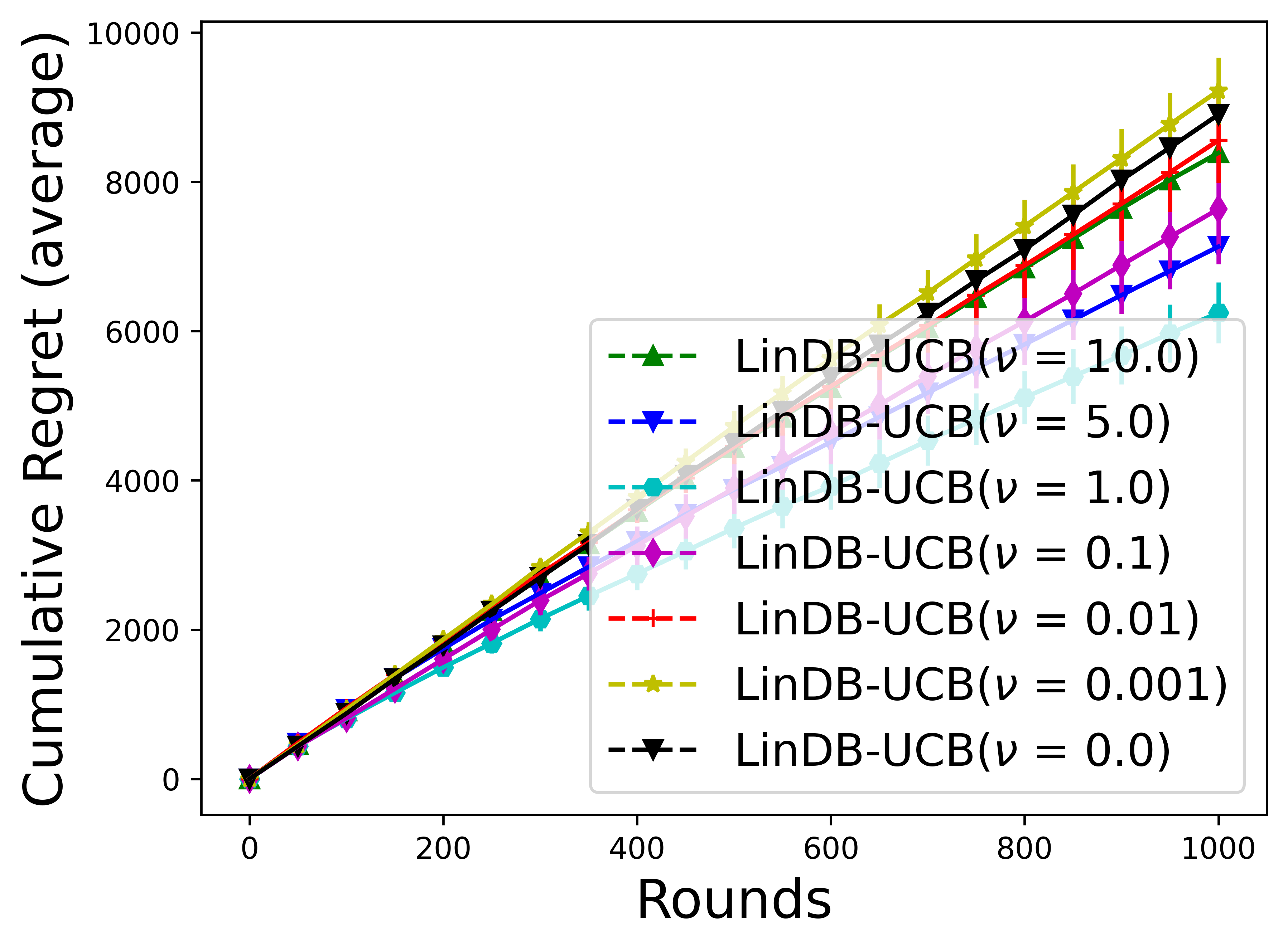
(a) Square (UCB)

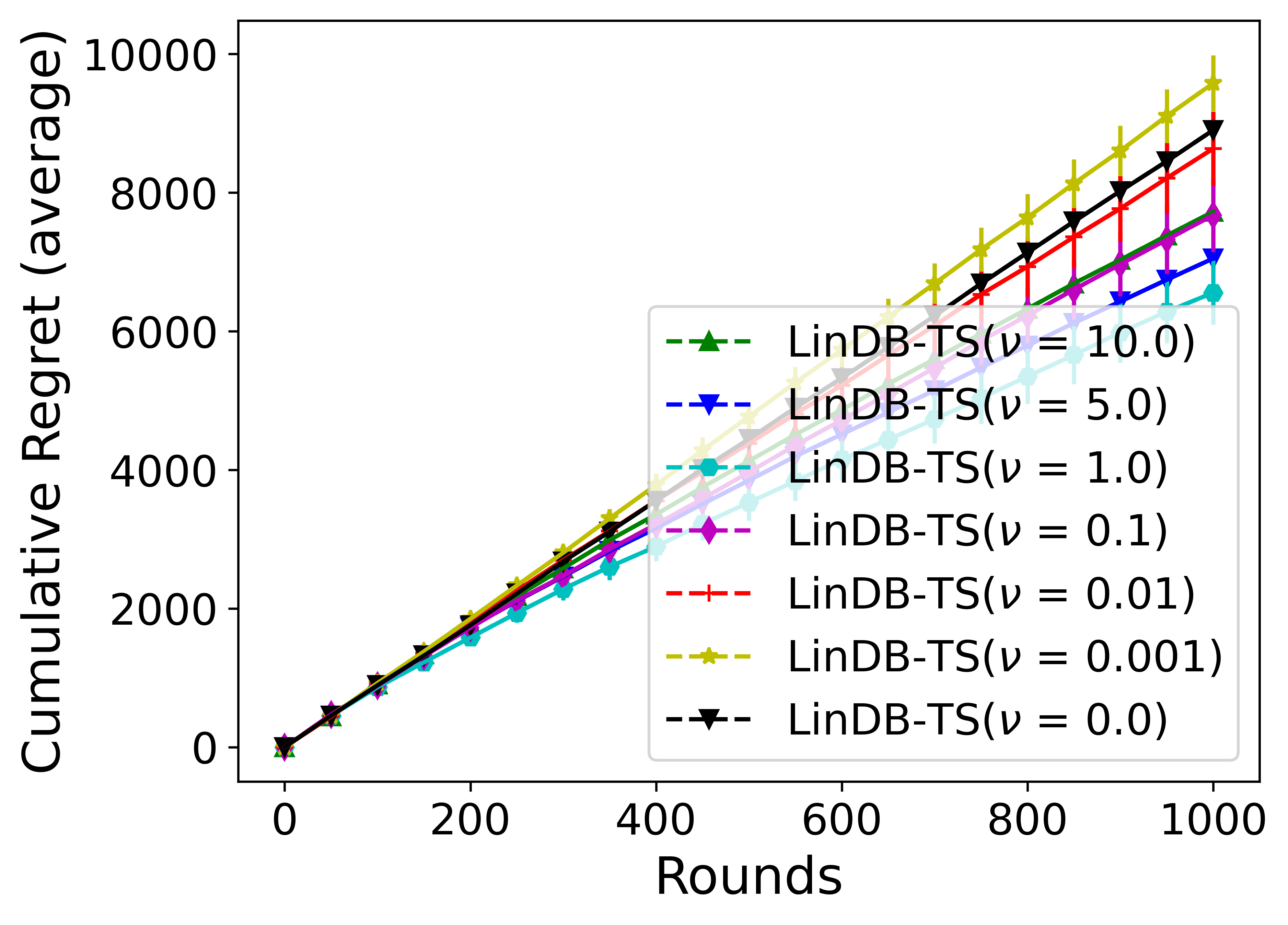
(b) Square (TS)

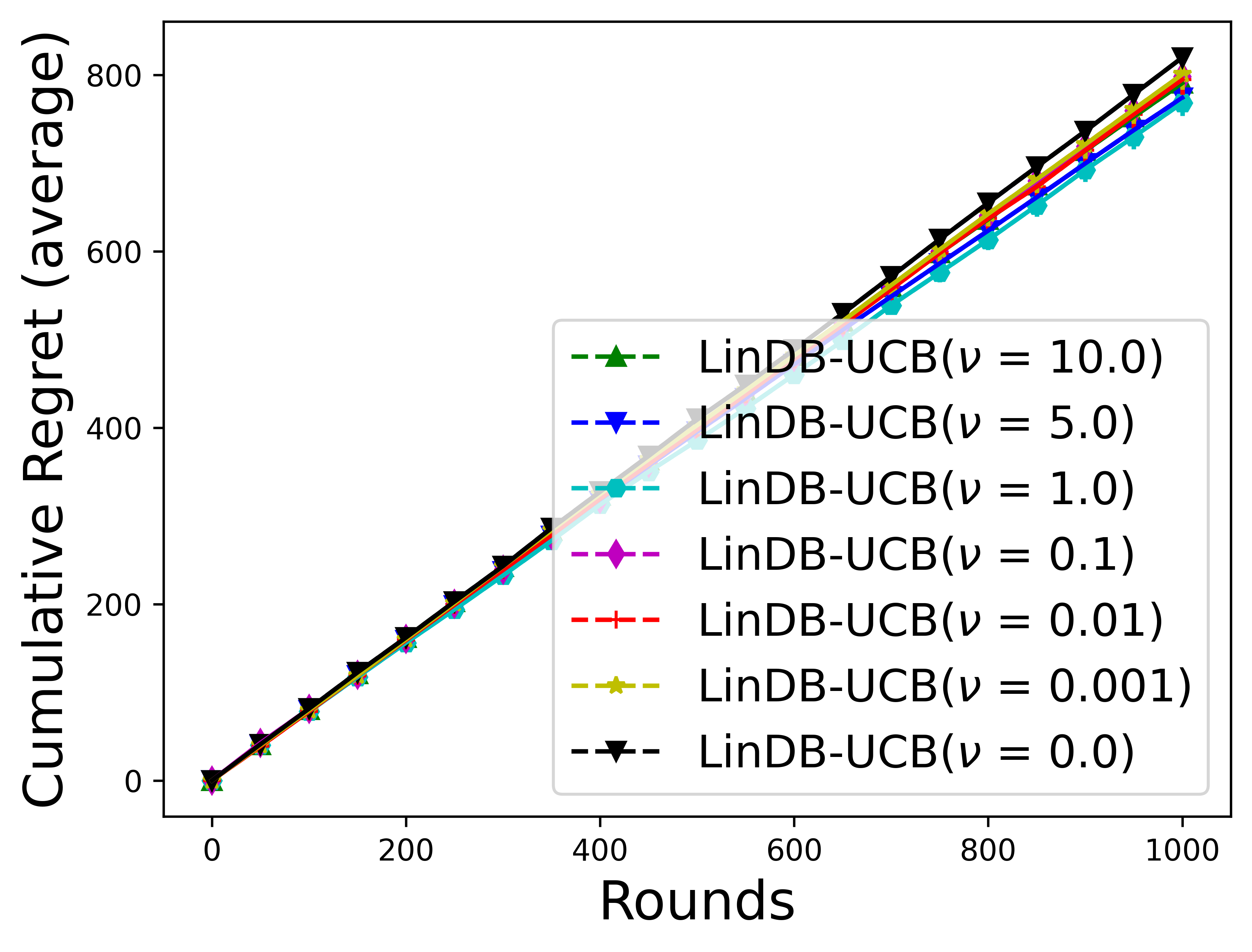
(c) Cosine (UCB)

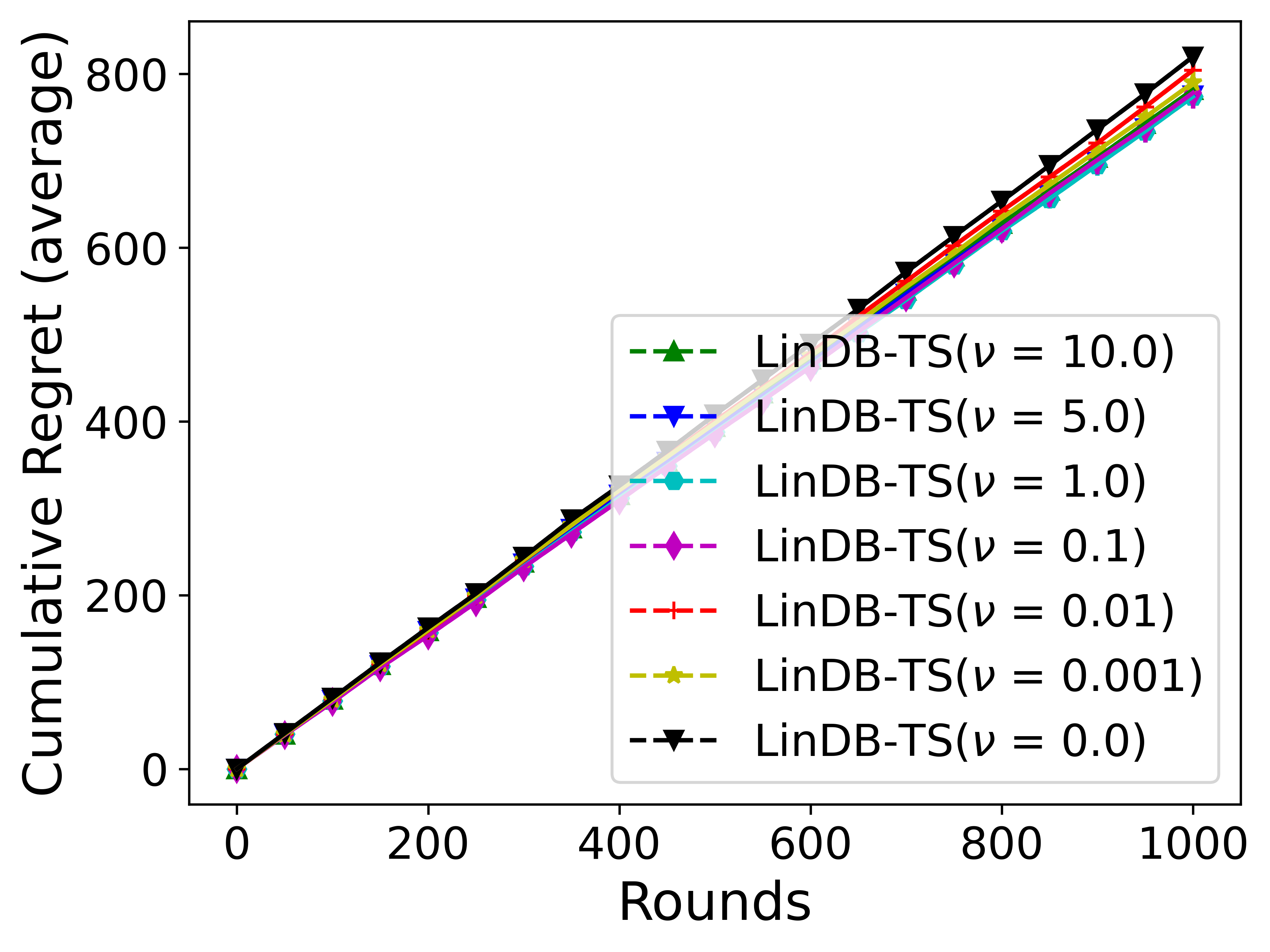
(d) Cosine (TS)

Figure 3: Average cumulative regret of LinDB-UCB and LinDB-TS vs. different values of $\nu$ for Square reward function $(i.e.,10(x^{\top}\theta)^{2})$.

(a) Varying $d$ (Average)

(b) Varying $d$ (Weak)

(c) Varying $K$ (Average)

(d) Varying $K$ (Weak)

Figure 4: Cumulative regret (average and weak) of NDB-TS vs. different number of arms $(K)$ and dimension of the context-arm feature vector $(d)$ for Square reward function $(i.e.,10(x^{\top}\theta)^{2})$.

(a) $10(x^{\top}\theta)^{2}$ (Average)

(b) $10(x^{\top}\theta)^{2}$ (Weak)

(c) $20(x^{\top}\theta)^{2}$ (Average)

(d) $20(x^{\top}\theta)^{2}$ (Weak)

(e) $30(x^{\top}\theta)^{2}$ (Average)

(f) $30(x^{\top}\theta)^{2}$ (Weak)

(g) $40(x^{\top}\theta)^{2}$ (Average)

(h) $40(x^{\top}\theta)^{2}$ (Weak)

Figure 5: Comparisons of cumulative regret (average and weak) of different dueling bandits algorithms for non-linear reward functions.

(a) $cos(3x^{\top}\theta)$ (Average)

(b) $cos(3x^{\top}\theta)$ (Weak)

(c) $3cos(x^{\top}\theta)$ (Average)

(d) $3cos(x^{\top}\theta)$ (Weak)

(e) $5cos(x^{\top}\theta)$ (Average)

(f) $5cos(x^{\top}\theta)$ (Weak)

(g) $10cos(x^{\top}\theta)$ (Average)

(h) $10cos(x^{\top}\theta)$ (Weak)

Figure 6: Comparisons of cumulative regret (average and weak) of different dueling bandits algorithms for non-linear reward functions.

(a) $10(x^{\top}\theta)^{2}$

(b) $40(x^{\top}\theta)^{2}$

(c) $cos(3x^{\top}\theta)$

(d) $10cos(x^{\top}\theta)$

Figure 7: Comparing cumulative regret of GLM bandits algorithms for non-linear reward functions.

(a) Varying $d$ (UCB)

(b) Varying $K$ (UCB)

(c) Varying $d$ (TS)

(d) Varying $K$ (TS)

Figure 8: Cumulative regret of Algorithm NCBF-UCB and NCBF-TS vs. different number of arms $(K)$ and dimension of the context-arm feature vector $(d)$ for Square reward function $(i.e.,10(x^{\top}\theta)^{2})$.

Appendix E Broader Impacts

The contributions of our work are primarily theoretical. Therefore, we do not foresee any immediate negative societal impact in the short term. Regarding our longer-term impacts, as discussed in Section 4, our algorithms can be potentially adopted to improve online RLHF. On the positive side, our work can lead to better and more efficient alignment of LLMs through improved online RLHF, which could benefit society. On the other hand, the potential negative societal impacts arising from RLHF may also apply to our work. On the other hand, potential mitigation measures to prevent the misuse of RLHF would also help safeguard the potential misuse of our algorithms.

References

- [1] Aadirupa Saha. Optimal algorithms for stochastic contextual preference bandits. In Proc. NeurIPS, pages 30050–30062, 2021.
- [2] Viktor Bengs, Aadirupa Saha, and Eyke Hüllermeier. Stochastic contextual dueling bandits under linear stochastic transitivity models. In Proc. ICML, pages 1764–1786, 2022.
- [3] Xuheng Li, Heyang Zhao, and Quanquan Gu. Feel-good thompson sampling for contextual dueling bandits. arXiv:2404.06013, 2024.
- [4] Lihong Li, Wei Chu, John Langford, and Robert E Schapire. A contextual-bandit approach to personalized news article recommendation. In Proc. WWW, pages 661–670, 2010.
- [5] Wei Chu, Lihong Li, Lev Reyzin, and Robert E Schapire. Contextual bandits with linear payoff functions. In Proc. AISTATS, pages 208–214, 2011.
- [6] Andreas Krause and Cheng S Ong. Contextual gaussian process bandit optimization. In Proc. NeurIPS, pages 2447–2455, 2011.
- [7] Dongruo Zhou, Lihong Li, and Quanquan Gu. Neural contextual bandits with UCB-based exploration. In Proc. ICML, pages 11492–11502, 2020.
- [8] Weitong Zhang, Dongruo Zhou, Lihong Li, and Quanquan Gu. Neural Thompson sampling. In Proc. ICLR, 2021.
- [9] Hossein Azari Soufiani, David Parkes, and Lirong Xia. Computing parametric ranking models via rank-breaking. In Proc. ICML, pages 360–368, 2014.
- [10] David R Hunter. Mm algorithms for generalized bradley-terry models. Annals of Statistics, pages 384–406, 2004.
- [11] R Duncan Luce. Individual choice behavior: A theoretical analysis. Courier Corporation, 2005.
- [12] Christopher KI Williams and Carl Edward Rasmussen. Gaussian Processes for Machine Learning. MIT press, 2006.
- [13] Niranjan Srinivas, Andreas Krause, Sham Kakade, and Matthias Seeger. Gaussian process optimization in the bandit setting: No regret and experimental design. In Proc. ICML, page 1015–1022, 2010.
- [14] Sayak Ray Chowdhury and Aditya Gopalan. On kernelized multi-armed bandits. In Proc. ICML, pages 844–853, 2017.
- [15] Zhongxiang Dai, Yao Shu, Arun Verma, Flint Xiaofeng Fan, Bryan Kian Hsiang Low, and Patrick Jaillet. Federated neural bandits. In Proc. ICLR, 2023.
- [16] Xiaoqiang Lin, Zhaoxuan Wu, Zhongxiang Dai, Wenyang Hu, Yao Shu, See-Kiong Ng, Patrick Jaillet, and Bryan Kian Hsiang Low. Use your instinct: Instruction optimization using neural bandits coupled with transformers. arXiv:2310.02905, 2023.
- [17] Peter Auer, Nicolo Cesa-Bianchi, and Paul Fischer. Finite-time analysis of the multiarmed bandit problem. Machine Learning, pages 235–256, 2002.
- [18] Yasin Abbasi-Yadkori, Dávid Pál, and Csaba Szepesvári. Improved algorithms for linear stochastic bandits. In Proc. NeurIPS, pages 2312–2320, 2011.
- [19] Lihong Li, Yu Lu, and Dengyong Zhou. Provably optimal algorithms for generalized linear contextual bandits. In Proc. ICML, pages 2071–2080, 2017.
- [20] Shipra Agrawal and Navin Goyal. Further optimal regret bounds for thompson sampling. In Proc. AISTATS, pages 99–107, 2013.
- [21] Shipra Agrawal and Navin Goyal. Thompson sampling for contextual bandits with linear payoffs. In Proc. ICML, pages 127–135, 2013.
- [22] Yisong Yue and Thorsten Joachims. Interactively optimizing information retrieval systems as a dueling bandits problem. In Proc. ICML, pages 1201–1208, 2009.
- [23] Yisong Yue and Thorsten Joachims. Beat the mean bandit. In Proc. ICML, pages 241–248, 2011.
- [24] Yisong Yue, Josef Broder, Robert Kleinberg, and Thorsten Joachims. The k-armed dueling bandits problem. Journal of Computer and System Sciences, pages 1538–1556, 2012.
- [25] Masrour Zoghi, Shimon A Whiteson, Maarten De Rijke, and Remi Munos. Relative confidence sampling for efficient on-line ranker evaluation. In Proc. WSDM, pages 73–82, 2014.
- [26] Nir Ailon, Zohar Karnin, and Thorsten Joachims. Reducing dueling bandits to cardinal bandits. In Proc. ICML, pages 856–864, 2014.
- [27] Masrour Zoghi, Shimon Whiteson, Remi Munos, and Maarten Rijke. Relative upper confidence bound for the k-armed dueling bandit problem. In Proc. ICML, pages 10–18, 2014.
- [28] Junpei Komiyama, Junya Honda, Hisashi Kashima, and Hiroshi Nakagawa. Regret lower bound and optimal algorithm in dueling bandit problem. In Proc. COLT, pages 1141–1154, 2015.
- [29] Pratik Gajane, Tanguy Urvoy, and Fabrice Clérot. A relative exponential weighing algorithm for adversarial utility-based dueling bandits. In Proc. ICML, pages 218–227, 2015.
- [30] Aadirupa Saha and Aditya Gopalan. Battle of bandits. In Proc. UAI, pages 805–814, 2018.
- [31] Aadirupa Saha and Aditya Gopalan. Active ranking with subset-wise preferences. In Proc. AISTATS, pages 3312–3321, 2019.
- [32] Aadirupa Saha and Aditya Gopalan. Pac battling bandits in the plackett-luce model. In Proc. ALT, pages 700–737, 2019.
- [33] Aadirupa Saha and Suprovat Ghoshal. Exploiting correlation to achieve faster learning rates in low-rank preference bandits. In Proc. AISTATS, pages 456–482, 2022.
- [34] Banghua Zhu, Michael Jordan, and Jiantao Jiao. Principled reinforcement learning with human feedback from pairwise or k-wise comparisons. In Proc. ICML, pages 43037–43067, 2023.
- [35] Viktor Bengs, Róbert Busa-Fekete, Adil El Mesaoudi-Paul, and Eyke Hüllermeier. Preference-based online learning with dueling bandits: A survey. Journal of Machine Learning Research, pages 1–108, 2021.
- [36] Aadirupa Saha and Akshay Krishnamurthy. Efficient and optimal algorithms for contextual dueling bandits under realizability. In Proc. ALT, pages 968–994, 2022.
- [37] Qiwei Di, Tao Jin, Yue Wu, Heyang Zhao, Farzad Farnoud, and Quanquan Gu. Variance-aware regret bounds for stochastic contextual dueling bandits. arXiv:2310.00968, 2023.
- [38] Olivier Chapelle and Lihong Li. An empirical evaluation of thompson sampling. In Proc. NeurIPS, pages 2249–2257, 2011.
- [39] Shreyas Chaudhari, Pranjal Aggarwal, Vishvak Murahari, Tanmay Rajpurohit, Ashwin Kalyan, Karthik Narasimhan, Ameet Deshpande, and Bruno Castro da Silva. Rlhf deciphered: A critical analysis of reinforcement learning from human feedback for llms. arXiv:2404.08555, 2024.
- [40] Yuntao Bai, Andy Jones, Kamal Ndousse, Amanda Askell, Anna Chen, Nova DasSarma, Dawn Drain, Stanislav Fort, Deep Ganguli, Tom Henighan, et al. Training a helpful and harmless assistant with reinforcement learning from human feedback. arXiv:2204.05862, 2022.
- [41] Jacob Menick, Maja Trebacz, Vladimir Mikulik, John Aslanides, Francis Song, Martin Chadwick, Mia Glaese, Susannah Young, Lucy Campbell-Gillingham, Geoffrey Irving, et al. Teaching language models to support answers with verified quotes. arXiv:2203.11147, 2022.
- [42] Viraj Mehta, Vikramjeet Das, Ojash Neopane, Yijia Dai, Ilija Bogunovic, Jeff Schneider, and Willie Neiswanger. Sample efficient reinforcement learning from human feedback via active exploration. arXiv:2312.00267, 2023.
- [43] Kaixuan Ji, Jiafan He, and Quanquan Gu. Reinforcement learning from human feedback with active queries. arXiv:2402.09401, 2024.
- [44] Nirjhar Das, Souradip Chakraborty, Aldo Pacchiano, and Sayak Ray Chowdhury. Provably sample efficient rlhf via active preference optimization. arXiv:2402.10500, 2024.
- [45] Kwang-Sung Jun, Aniruddha Bhargava, Robert Nowak, and Rebecca Willett. Scalable generalized linear bandits: Online computation and hashing. In Proc. NeurIPS, pages 99–109, 2017.
- [46] Louis Faury, Marc Abeille, Clément Calauzènes, and Olivier Fercoq. Improved optimistic algorithms for logistic bandits. In Proc. ICML, pages 3052–3060, 2020.
- [47] Parnian Kassraie and Andreas Krause. Neural contextual bandits without regret. In Proc. AISTATS, pages 240–278, 2022.
- [48] Arthur Jacot, Franck Gabriel, and Clément Hongler. Neural tangent kernel: Convergence and generalization in neural networks. Proc. NeurIPS, pages 8580–8589, 2018.