Covering a Graph with Dense Subgraph Families, via Triangle-Rich Sets

Abstract.

Graphs are a fundamental data structure used to represent relationships in domains as diverse as the social sciences, bioinformatics, cybersecurity, the Internet, and more. One of the central observations in network science is that real-world graphs are globally sparse, yet contains numerous “pockets" of high edge density. A fundamental task in graph mining is to discover these dense subgraphs. Most common formulations of the problem involve finding a single (or a few) “optimally" dense subsets. But in most real applications, one does not care for the optimality. Instead, we want to find a large collection of dense subsets that covers a significant fraction of the input graph.

We give a mathematical formulation of this problem, using a new definition of regularly triangle-rich (RTR) families. These families capture the notion of dense subgraphs that contain many triangles and have degrees comparable to the subgraph size. We design a provable algorithm, RTRExtractor, that can discover RTR families that approximately cover any RTR set. The algorithm is efficient and is inspired by recent results that use triangle counts for community testing and clustering.

We show that RTRExtractor has excellent behavior on a large variety of real-world datasets. It is able to process graphs with hundreds of millions of edges within minutes. Across many datasets, RTRExtractor achieves high coverage using high edge density datasets. For example, the output covers a quarter of the vertices with subgraphs of edge density more than (say) $0.5$, for datasets with 10M+ edges. We show an example of how the output of RTRExtractor correlates with meaningful sets of similar vertices in a citation network, demonstrating the utility of RTRExtractor for unsupervised graph discovery tasks.

1. Introduction

Coverage

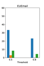
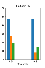
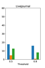
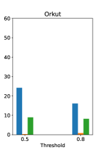
Figure 1. Coverage of RTRExtractor compared to the two best performing competitors in a variety of networks of different sizes: from thousands to millions of vertices. For each method, we compute the fraction of vertices in sets of 5 vertices or more, and of density more than 0.5 and 0.8. RTRExtractor consistently covers significantly higher percentages in dense clusters.

Graphs are a fundamental data structure used to represent relationships in domains as diverse as the social sciences, bioinformatics, cybersecurity, the Internet, and more. One of the central observations in network science is that real-world graphs are globally sparse, yet contains numerous “pockets" of density. A fundamental task in graph mining is to discover these dense subgraphs (Lee et al., 2010).

Dense subgraph discovery has a rich set of applications. It has been used for finding cohesive social groups (Beal et al., 2003; Forsyth, 2010), spam link farms in web graphs (Kumar et al., 1999; Dourisboure et al., 2007; Gibson et al., 2005), graph visualization (Alvarez-hamelin et al., 2005), real-time story identification (Angel et al., 2012), DNA motif detection in biological networks (Fratkin et al., 2006), finding correlated genes (Zhang and Horvath, 2005), epilepsy prediction (Iasemidis et al., 2003), finding price value motifs in financial data (Du et al., 2009), graph compression (Buehrer and Chellapilla, 2008), distance query indexing (Jin et al., 2009), and increasing the throughput of social networking site servers (Gionis et al., 2013). Dense subgraph discovery is a typical unsupervised machine learning task and a central tool for knowledge/structure discovery in large networks.

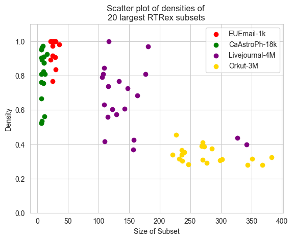
Figure 2. The largest 20 RTRExtractor subsets produced on some datasets. and their respective densities. We note that even for the largest subsets, which in some cases may have hundreds of vertices, density is still remarkably high.

There are numerous challenges in designing algorithms in the context of the above applications. Consider the input graph $G=(V,E)$. The density of a subset $S\subset V$ is $E(S)/{|S|\choose 2}$, where $E(S)$ is the number of edges inside $S$. The density has a maximum value of $1$, when $S$ is a clique. The typical density of a real-world (say) social network with millions of vertices is less than $10^{-5}$, but there are often sets of size (say) $20$ with density above $0.5$. Our aim is to find sufficiently large sets that are sufficiently dense (in practice, tens to few hundreds of vertices and density $0.3$ or above).

Most of the algorithms and data mining literature phrase this as an optimization problem (Goldberg, 1984), either finding the largest set above a given density, or finding the densest set above or below a given size (Andersen and Chellapilla, 2009). Another popular variant is related to the notion of correlation clustering (Bansal et al., 2004), which has received a lot of theoretical attention in recent years. Typical formulations are NP-hard (Håstad, 1999; Feige, 2002; Khot, 2006), and most practical procedures use heuristics and approximation algorithms (Charikar, 2000; Andersen and Chellapilla, 2009; Boob et al., 2020; Tsourakakis, 2015, 2014; Konar and Sidiropoulos, 2022; Danisch et al., 2017; Chekuri et al., [n.d.]). In the past decade, the problem of finding one or many dense subgraphs has been approached in various forms by the data mining community (Bonchi et al., 2021; Sotirov, 2020; Gibson et al., 2005; Shin et al., 2016); we refer the reader to the recent survey by Lanciano et al. for a more comprehensive list (Lanciano et al., 2023). From the viewpoint of applications and as an unsupervised ML technique, this formulation has shortcomings for real-world networks. The vanilla densest-subgraph variant is prone to extracting massive subgraphs, the work on $k$-way cuts asks for a specific, prescribed $k$ as the number of partitions, and $k$-densest subgraphs ask for a lower bound on the size of each partition (and the best known approximation factors are quite poor). One rarely cares about the exact (or even approximate) optimum. Since data has noise, it is possible that a worse solution is still meaningful. Moreover, applications require finding many possible solutions. From a knowledge discovery perspective, if a dense set of vertices indicates special structure, we would like to find many such sets. Even if we do not capture the single optimal dense set exactly, we would like to learn about as many dense sets as possible. Often each dense set represents some "information" or structure to be discovered, so we want a large disjoint collection of such sets. Dense subgraphs (Alsentzer et al., 2020; Frasca et al., 2022) are used as primitives for downstream ML-tasks, so the ability to cover more vertices in dense subgraphs would be an obvious benefit.

Our goal for this paper is the following. Can we design algorithms that cover a significant portion of the graph, using disjoint large, high density subgraphs? From an empirical standpoint, we want an algorithm that can scale to graphs with hundreds of millions of edges, and can find many dense subgraphs in real data. Towards this goal, we would like a theoretical framework that leads to practical and provable algorithms. Can we give a formal setup, where many dense subgraphs can be found tractably?

1.1. Our Contributions

We give a new theoretical setup for dense subgraph discovery, accounting for triangle density. We design an algorithm, RTRExtractor, that is a provable (approximation) algorithm for this version of dense subgraph discovery. We show that an implementation of RTRExtractor is extremely successful at finding many dense subgraphs in a variety of real-world datasets.

$|T|\geq$	EUEmail	Hamsterster	CaAstroPh	Epinions	DBLP	Youtube	Skitter	Wiki	LJ	Orkut
10	0.82	0.97	0.99	0.87	1.0	0.89	0.74	0.76	0.89	0.85

Table 1. Mean edge density in RTRExtractor output sets of size at least 10. Amazon has no output sets with $10$ vertices.

Formulation through triangle-rich sets.

Inspired by many results that exploit triangles to find dense subgraphs, we define the notion of “regularly triangle-rich" (RTR) sets. These are subsets of vertices of comparable degree that contain many triangles. These sets are significantly more restrictive than high edge density sets. The utility of this definition is that we can prove strong theoretical guarantees on algorithms. Our actual empirical goal is not recovering RTR sets, but we discover that it is a good guide for getting practical dense subgraph discovery algorithms.

Theoretical algorithm and analysis.

We can prove a strong "recovery" guarantee, using the RTR framework. We design an algorithm, RTRExtractor, that outputs a disjoint family of RTR sets. A constant fraction of every RTR set is contained in the family. Under some stronger conditions on the RTR set, a constant fraction of the set is actually contained in a single output of RTRExtractor. We borrow tools from theoretical work on triangle-dense decompositions of graphs to design RTRExtractor (Gupta et al., 2014).

Fast implementation of RTRExtractor.

We give a practical implementation of RTRExtractor, with some heuristics to improve the coverage. (The code is available at (rtr, 2024).) As stated earlier, our aim is to cover a large portion of the graph with dense subgraphs. We experiment on a large collection of real-world, publicly available datasets. RTRExtractor runs extremely fast on large graphs and outputs a large collection of dense subgraphs on real-world graphs.

High coverage in practice.

For example, on a large Orkut social network with more than a hundred million edges, RTRExtractor covers a quarter of the graph with subgraph of density more than $0.5$. We consistently observe this behavior across many datasets we experiment with. We compare RTRExtractor against a number of state of the art dense subgraph discovery algorithms and community detection procedures (the Louvain algorithm (Blondel et al., 2008), iterated Flowless (Boob et al., 2020), iterated greedy (Charikar, 2000), and the nucleus decomposition (Sariyuce et al., 2015)). Nucleus decompositions are the only algorithm specifically tailored to finding large families of dense subgraphs. (We discuss more in §2.) In Fig. 1, we compare the number of vertices covered by each method, using sets of more than a given density. Across almost all datasets, RTRExtractor gets higher coverage of dense subgraphs compared to all these algorithms.

Finding many large dense subgraphs.

In Fig. 2, we show the size and density of the 20 largest sets output by RTRExtractor on various datasets. In all datasets, we see that RTRExtractor can get numerous, large, dense sets. On the Orkut social network with 3M vertices, we get more than 20 sets of size more than 200, with edge density more than 0.3. In Tab. 1, we give the mean density of output sets of size at least 10 vertices. We see the extremely high densities; in the case of the DBLP dataset, almost every output set is a clique (density of 0.1).

Qualitative examination of subsets.

We also demonstrate the semantic significance of the output family. RTRExtractor is able to output sets of similar vertices in labelled networks without any knowledge of the labels. For a DBLP citation network dataset (Tang et al., 2008), RTRExtractor outputs a family of sets of papers. We manually inspect these sets and see that they are always on a single subtopic. These results reinforce the need to have dense subgraph discovery algorithms that output many sets.

2. Related Work

Finding the densest subgraph is a problem that has attracted a lot of attraction from both theoretical and applied researchers. It is of theoretical interest because most formulations are NP hard, and a lot of research has gone into approximation algorithms; indeed, there exist linear time approximation algorithms due to Asahiro (Asahiro et al., 2002), Charikar (Charikar, 2000) and Tsourakakis (Tsourakakis, 2014) that have received a lot of attention. Other efficient algorithms in practice include more recent work in data mining  (Tsourakakis, 2015; Boob et al., 2020) leveraging cliques, quasi-cliques, as well as approaches based on cores and trusses  (Andersen and Chellapilla, 2009; Wang et al., 2010; Wang and Cheng, 2012; Huang and Lakshmanan, 2017; Xu et al., 2023). A growing group of results use triangle information for algorithmic purposes (Sariyuce et al., 2015; Tsourakakis, 2015; Benson et al., 2016; Tsourakakis et al., [n.d.]; Veldt et al., [n.d.]). We point the readers to a number of surveys on dense subgraph discovery  (Lee et al., 2010; Lanciano et al., 2023; Fang et al., 2020).

A distinct but related problem is the one of community detection. While definitions of communities vary, it is widely accepted that dense subgraphs are closely related to real world communities in networks (Leskovec et al., 2008; Chen and Saad, 2012). One of the most celebrated algorithms in this field is the Louvain algorithm (Blondel et al., 2008), which does a local maximization of the modularity metric due to Newman and Girvan (Girvan and Newman, 2002). The recent work of Miyauchi and Kawase (Miyauchi and Kawase, 2015), and the later work of Miyauchi and Kakimura (Miyauchi and Kakimura, 2018) use metrics related to modularity to find dense subgraphs in networks. Other popular methods include Infomap (Rosvall and Bergstrom, 2008) and other approaches based on the map equation (Rosvall et al., 2009), the Leiden algorithm,  (Traag et al., 2019), label propagation (Raghavan et al., 2007). The survey by Jin et al. (Jin et al., 2021) takes a detailed look at different community detection methods from statistical modelling to the more recent deep learning based methods.

Most relevant to our work is the result of Gupta, Roughgarden, and Seshadhri (Gupta et al., 2014). They prove a decomposition theorem for triangle-rich graphs, as measured by graph transitivity. Their main result shows that a triangle-dense graph can be clustered into dense clusters. In a recent result, a spectral connection to this was found in the work of Basu, Bera and Seshadhri (Basu et al., 2023), which involved generalizations of their proof technique using the normalized adjacency matrix. Our main insight is that the algorithm of Gupta et al can adapted to extract our stronger notion of RTR sets. Moreover, we can prove explicit approximation guarantees on the output. We also note that while we present a scalable implementation,  (Gupta et al., 2014) only give a theoretical algorithm and no implementation.

3. The main problem

Consider an input simple graph $G=(V,E)$. Our high level objective is to output many sets that are “dense". We need to define our density objective.

The typical notion of density of a subset $S\subseteq V$ of vertices is the edge density $E(S)/{|S|\choose 2}$, where $E(S)$ the number of edges contained in $S$. Note that this definition is interesting only when $|S|$ is large, and hence algorithms finding useful dense subgraphs also need to optimize for size. Another less common notion of density is $E(S)/|S|$, the average degree inside $S$. While it is easy to optimize for this notion, the output often has poor edge density and consists of extremely large sets. As we discuss in §7, practical algorithms that optimize for these quantities give poor results (even in terms of edge density).

Our starting point is that the best possible dense subgraph is an isolated clique. For example, a (say) clique of size 15 formed by vertices of degree (say) 1000 is not an ideal dense subgraph. We want our definitions to account for the degrees of the vertices involved in the dense set. While edge density captures the desired objective in practice, it is not mathematically ideal. First, the isolated edge is an optimum. Moreover, suppose $S$ was (internally) a dense bipartite graph. It could have edge density as high as $0.5$, but does not really conform with our usual notion of dense substructure. We would like high internal clustering coefficients as well. The intuition is repeatedly observed, where using triangles leads to better density/community/clustering outcomes in practice  (Sariyuce et al., 2015; Tsourakakis, 2015; Benson et al., 2016; Tsourakakis et al., [n.d.]).

Obviously, an isolated clique of vertices is the best possible dense subgraph. We want our dense subgraphs to share the characteristics of an isolated clique, as much as possible. These considerations motivate our definition of regularly triangle-rich sets.

First, we give the standard definition of triangle density.

Definition 3.1.

The triangle density of a set $S$ of vertices is the number of triangles contained in $S$ divided by ${|S|\choose 3}$.

The next definition is the central notion of this paper.

Definition 3.2.

Let $\alpha\in[0,1]$. A set $S$ of vertices is called $\alpha$-regularly triangle-rich if (i) all vertices in $S$ have (total) degree in $[\alpha|S|,|S|/\alpha]$, and (ii) the triangle density of $S$ is at least $\alpha$.

We note that triangle density implies edge density due to Túran-type theorems, so an $\alpha$-regularly triangle-rich set also has edge density $\alpha$. Observe that the degree in the above definition refers to degree in the original graph, not just in the set $S$. Thus, the total degrees are comparable to set size itself. A $1$-regularly triangle-rich set $S$ is necessarily an isolated clique, the perfect dense subgraph. One can think of $\alpha$ as a measure of how close a set $S$ is to being an isolated clique, where we account for both internal triangle density and the degree regularity. Our focus is on the setting when $\alpha$ is a constant, like (say) $0.5$ or $0.8$. For the sake of mathematical analysis, we will use the (standard) terminology $\Omega(1)$-regularly triangle-rich to denote “constant"-regularly triangle-rich sets.

The primary utility of this definition is shown by our algorithmic results. The results give guarantees on the output of RTRExtractor, our main procedure given in Alg. 1. RTRExtractor outputs a family $\mathcal{T}$ of disjoint sets. RTRExtractor can “weakly discover" all $\Omega(1)$-regularly triangle-rich sets in a graph.

Theorem 3.3.

Consider an input graph $G=(V,E)$. For any constant $\alpha$, there exists input parameters for the algorithm RTRExtractor with the following guarantees. (i) RTRExtractor outputs a disjoint family of sets $\mathcal{T}$, such that each set is $\Omega(1)$-regularly triangle-rich. (ii) For any $S$ that is $\alpha$-regularly triangle-rich, a least a constant fraction of $S$ is contained in $\mathcal{T}$. (All constants have polynomial dependencies on $\alpha$.)

(The running time of RTRExtractor is, up to constant factors, the time taken to list all triangles of $G$.)

This is a strong guarantee, since every $\Omega(1)$-regularly triangle-rich set $S$ is approximately captured by the output $\mathcal{T}$. The output itself is a disjoint family of $\Omega(1)$-regularly triangle-rich sets. Note that we do not (and cannot) guarantee that $S$ is approximately captured by a single (or few) sets of $\mathcal{T}$. This is because regularly triangle-rich sets can be overlapping, and for a disjoint family $\mathcal{T}$ of regularly triangle-rich sets, some other $\Omega(1)$-rtr set is split among many sets of $\mathcal{T}$.

Here are some examples showing these situations. Consider a graph formed by as follows. We first take $k$ disjoint $k$-cliques. Then, we take a single vertex from each of these cliques, and form a $k$-clique $C$ inside it. There are now $(k+1)$ $k$-cliques, and each of them is $1/2$-regularly triangle-rich. (The $1/2$ is because the degrees are either $k-1$ or $2(k-1)$.) A perfectly reasonable $\mathcal{T}$ is to output the set of $k$ disjoint $k$-cliques. But then $C$ would be split among different sets in $\mathcal{T}$. Theorem 3.3 asserts that, regardless of the graph structure, every $\Omega(1)$-regularly triangle-rich set has a constant factor of its vertices in $\mathcal{T}$, which is itself a family of $\Omega(1)$-regularly triangle-rich sets.

It is natural to ask if there are stronger assumptions under which an $\Omega(1)$-regularly triangle-rich set is roughly contained in one (or $O(1)$) sets in $\mathcal{T}$.

Definition 3.4.

Let $\alpha>\beta$. An $\alpha$-regularly triangle-rich $S$ is called $\beta$-well separated if: for all edges $(u,v)$ containing at least one vertex in $S$, the edge contains at most $\beta|S|$ triangles where the third vertex is outside $S$.

So edges contained in a well-separated regularly triangle-rich set have few triangles “leaving" $S$. This is similar to a triangle cut constraint, used in previous work  (Tsourakakis et al., [n.d.]; Benson et al., 2016). For any well separated regularly triangle-rich set $S$, we can prove a stronger condition: there exists an output set $\mathcal{T}$ (of RTRExtractor) that contains a constant fraction of $S$.

Theorem 3.5.

Consider any $\alpha$-regularly triangle-rich set $S$ that is $\beta$-well separated, for constants $\alpha,\beta$, where $\beta$ is sufficiently small (compared to $\alpha$). Then, there exist input parameters for the algorithm RTRExtractor such that the output $\mathcal{T}$ has a set that contains an $\Omega(1)$-fraction of $S$.

Connection to coverage.

As said earlier, in practice, we care for the coverage. Theorem 3.3 and Theorem 3.5 do not explicitly give coverage guarantees, but there are implicitly implied. Suppose a large portion of the graph $G$ can be covered by disjoint $\Omega(1)$-regularly triangle-rich sets. A constant fraction of each of these sets is present in the output of RTRExtractor, so the output will have good coverage. (And each output set is regularly triangle-rich, so the graph is covered with dense sets.) The "real" validation is done through our experiments in §7.

4. The Main Ideas Behind RTRExtractor

We describe the main procedure, RTRExtractor. The inspiration for RTRExtractor is the theoretical decomposition results of Gupta, Roughgarden, and Seshadhri (Gupta et al., 2014). (We stress that (Gupta et al., 2014) is purely theoretical and has no empirical results.) The main idea, which is itself present in numerous results, is to use the triangles to guide a local extraction of a dense “cluster" (Sariyuce et al., 2015; Tsourakakis, 2015; Benson et al., 2016; Tsourakakis et al., [n.d.]).

We use $d_{v}$ to denote the degree of $v$ in the input graph $G$.

Algorithm 1 RTRExtractor$(G,\varepsilon,\beta)$: (We use $d_{v}$ to denote the degree of $v$ in the input graph $G$.)

1:Initialize an empty family $\mathcal{T}$.

2:Initialize subgraph $H$ to $G$.

3:while $H$ is non-empty do

4:     while there is edge $e=(u,v)$ in $<\varepsilon(d_{u}+d_{v})$ triangles in $H$ do

5:         Delete $e$ from $H$.

6:     end while

7:     Delete all isolated vertices from $H$.

8:     Pick a vertex $v$ in $H$ with lowest $d_{v}$.

9:     Construct $N$, the neighborhood of $v$ in $H$.

10:     Let set $T=\{v\}\cup N$.

11:     for every vertex $u$ that is a neighbor of $N$ do

12:         Let $t_{u}$ be the number of triangles (in $H$) from $u$ to $N$.

13:         If $t_{u}>\beta d^{2}_{v}$ , add $u$ to $T$.

14:     end for

15:     Delete $T$ from the subgraph $H$.

16:     Add set $T$ to output family $\mathcal{T}$.

17:end while

18:Output $\mathcal{T}$.

The procedure RTRExtractor takes two arguments $\varepsilon,\beta$ that are thresholds used at two separate steps. In the theorems, these (constant) parameters are chosen appropriate for the analysis. In practice, we set these to simple fixed values. Also, the practical implementation differs somewhat from the theoretical description, but that is mostly for convenience. We discuss these practical aspects in §6. In this section, our focus is on the theoretical aspects and intuition for RTRExtractor.

RTRExtractor goes through an iterated extraction process. First, there is a “cleaning" step (Step 5) that removes edges in few triangles, yielding subgraph $H$. The main work is finding an regularly triangle-rich set $T$ in $H$. This set is removed from $H$. The resulting $H$ is again cleaned, the next regularly triangle-rich set is found, and so on. We refer to the process of each output set $T$ being removed as an extraction.

The cleaning operation of Step 5 removes edges that are present in too few triangles. Intuitively, these are edges that may “distract" the subsequent extraction, so we delete them. The parameter $\varepsilon$ is used to determine this threshold. Observe that $d_{u}+d_{v}$ is an upper bound on the number of triangles that the edge $(u,v)$ participates in. Step 5 computes the fraction of triangles that $(u,v)$ participates in with respect to this simple upper bound. That fraction is used as a threshold. Note that the total number of triangles that $(u,v)$ participates in is at most $\min(d_{u},d_{v})$, so this step automatically removes edges between vertices of disparate degrees.

The cleaning of Step 5, while quite simple, is an immensely useful algorithmic (and practical) idea. In a cleaned graph, the neighborhood of a vertex is automatically rich in triangles. So a simple BFS based algorithm can extract out dense (and triangle-rich) sets. While this idea has appeared in theory and some practical results  (Satuluri et al., [n.d.]), it has been underutilized as a technique for dense subgraph discovery.

After cleaning, RTRExtractor takes the lowest degree vertex $v$ in the current subgraph $H$, and start a “seeded" extraction from $v$. At this point, all edges participate in sufficiently many triangles. So the neighborhood $N$ of $v$ also contains enough triangles, and we set $T$ as $\{v\}\cup N$. If we simply extract $T$ as a set, we run the risk of destroying too many triangle-rich sets. The main insight is that we need to extract sets of radius $2$.

We give a simple justification. Suppose $G$ is a regular complete tripartite graph, so the vertices are partitioned into three equal sized sets $V_{1},V_{2},V_{3}$, with all edges between sets. If $v\in V_{1}$, then $\{v\}\cup N$ essentially consists of $V_{2}\cup V_{3}$. Removing this set would destroy all the edges (and triangles) incident to $V_{1}\setminus\{v\}$. All vertices in $V_{1}$ would become singletons, which is a bad output. More generally, dense subgraphs (like dense Erdős-Rényi graphs) often have radius $2$. If $G$ was just a single uniformly dense random graph, extracting neighborhoods would not suffice.

So RTRExtractor looks at the neighbors of $N$, the two-hop neighborhood from $v$. The key insight is to find vertices in the two-hop neighborhood that form sufficiently many triangles with the neighborhood $N$. The argument $\beta$ is used as a threshold to determine which vertices are added to $T$. This parameter is critical to get two-hope neighborhoods that are triangle-rich. Vertices not assigned to any output set $T$ are considered singletons.

4.1. Challenges in the analysis

There are two parts to the analysis. The first part shows that the output of RTRExtractor is a family of regularly triangle-rich sets. The second part shows that a given regularly triangle-rich set $S$ is approximately captured, either in weak sense of Theorem 3.3 or the stronger sense of Theorem 3.5. There is a tension between these goals. To output regularly triangle-rich sets, the cleaning of Step 5 needs to be aggressive enough to delete edges that reduce triangle density. Also, Step 13 adds vertices to a set that is already triangle-rich, and hence we want it to be stringent. But these are exactly the opposite of what is needed to preserve an existing triangle-rich set $S$. The clean operation could delete edges from $S$, making vertices in $S$ disconnected in $H$. Moreover, we would need Step 13 to add in many vertices, to preserve as much of $S$. The main point of the analysis is to prove that this tension can be resolved, with the right arguments $\varepsilon$ and $\beta$.

One of the insights of this analysis is that an accounting in terms of triangles is more powerful than keeping track of edges and density. As we described earlier, Step 5 is a central operation to ensure that the output is triangle-rich (and hence dense). Iterated with extraction steps, it might destroy an existing regularly triangle-rich $S$. As various extractions proceeds, they may remove a few vertices of $S$. These removals affect the internal structure in $S$ by deleting triangles. Hence, subsequent cleaning operations could end up deleting large portions of $S$, affecting the desired guarantees of Theorem 3.3 and Theorem 3.5.

We prove that the regularly triangle-rich definition ensures that there is a “core" of $S$ that is not affected by deletions of vertices outside the core. The only way that RTRExtractor can delete the core is by extracting vertices into the output sets $T$. Moreover, using the well-separated condition of Definition 3.4, we can show any extraction that removes even a single vertex of the core must remove a constant fraction of $S$. These arguments crucially use Step 13 to ensure that extractions that (say) seeded in $S$ must cover a significant fraction of $S$.

5. Analysis

The first step in the analysis is to show that every set output by RTRExtractoris $\Omega(1)$-regularly triangle-rich. For convenience, we think of the input arguments $\varepsilon,\beta$ to constants, so we use $\Omega(1)$ notation to suppress dependencies on these values. We also consider the $\alpha$ parameter (in Definition 3.2) to be a constant. All constants will have at most polynomial dependencies on each other. We do not try to optimize these dependencies, so our mathematical analysis is focused on the asymptotics. In practice, we set these parameters to be $0.1,0.3,0.5$, etc. So assuming they are constant is consistent with our experiments. (The true “test" of RTRExtractor is the strong experimental results.)

Lemma 5.1.

Every $T$ output by RTRExtractor$(\varepsilon,\beta)$ is $\Omega(\mathrm{poly}(\varepsilon,\beta))$-regularly triangle-rich. Hence, if $\varepsilon,\beta=\Omega(1)$, then every $T$ output is $\Omega(1)$-regularly triangle-rich.

Proof.

Consider some output set $T$. Suppose it is removed from subgraph $H$, starting from a seed vertex $v$. In all calculations that follow, we are considering the properties of the subgraph $H$. A crucial property is that every edge $(x,y)$ in $H$ participates in at least $\varepsilon(d_{x}+d_{y})$ triangles. Moreover, all degrees are at least $d_{v}$.

Since $v$ has non-zero degree in $H$, there is some edge $(u,v)$ in $H$. The edge $(u,v)$ participates in at least $\varepsilon(d_{u}+d_{v})$ triangles in $H$. Observe that the number of triangles is at most $\min(d_{u},d_{v})=d_{v}$. Thus, $\varepsilon(d_{u}+d_{v})\leq d_{v}$, implying $d_{u}\leq d_{v}/\varepsilon$. In general, for any edge $(x,y)$ in $H$, $d_{x}=\Theta(d_{y})$. For any arbitrary vertex in the two-hop neighborhood, the degree is at most $d_{v}/\varepsilon^{2}$.

Since $(u,v)$ participates in more than $\varepsilon d_{v}$ triangles in $H$, $v$ must have at least $\varepsilon d_{v}$ neighbors in $H$. Moreover, every edge $(u^{\prime},v)$ participates in at least $\varepsilon d_{v}$ triangles. Thus, $v$ participates in at least $\varepsilon^{2}d^{2}_{v}/2$ triangles ($\varepsilon d_{v}$ triangles along every edge $(u^{\prime},v)$, and each triangle is counted at most twice). Every triangle incident to $v$ corresponds to an edge in the neighborhood $N$ of $v$. So $N$ contains $\varepsilon^{2}d^{2}_{v}/2$ edges. Every edge participates in at least $\varepsilon d_{v}$ triangles. Hence, there are at least $\varepsilon^{3}d^{3}_{v}/2$ triangles with at least two vertices in $N$.

Hence, $\sum_{u}t_{u}\geq\varepsilon^{3}d^{3}_{v}/2$. For every $u$, let $b_{u}$ be the number of neighbors of $u$ in $N$. Observe that $t_{u}\leq b^{2}_{u}$, since every triangle that $u$ forms with $N$ is made by a pair of neighbors in $N$. Thus, $\sum_{u}\sqrt{t_{u}}\leq\sum_{u}b_{u}$. The term $\sum_{u}b_{u}$ counts the number of edges incident to $N$. The size of $N$ is at most $d_{v}$, and each vertex in $N$ has degree at most $d_{v}/\varepsilon$ (as shown earlier). So $\sum_{u}\sqrt{t_{u}}\leq\sum_{u}b_{u}\leq d^{2}_{v}/\varepsilon$.

Consider the sum $\sum_{u:t_{u}<\varepsilon^{8}d^{2}_{v}/9}t_{u}$. We can bound this as follows:

$$\sum_{u:t_{u}<\varepsilon^{8}d^{2}_{v}/9}t_{u}=\sum_{u:t_{u}<\varepsilon^{8}d^{2}_{v}/9}\sqrt{t_{u}}\sqrt{t_{u}} \leq (\varepsilon^{4}/3)d_{v}\sum_{u}\sqrt{t_{u}}$$

$$\leq (\varepsilon^{4}/3)d_{v}\cdot d^{2}_{v}/\varepsilon=\varepsilon^{3}d^{3}_{v}/3$$

Thus, for $\beta=\varepsilon^{8}/9$, we get that $\sum_{u:t_{u}\geq\beta d^{2}_{v}}t_{u}\geq\varepsilon^{3}d^{3}_{v}/2-\varepsilon^{3}d^{3}_{v}/3=\Omega(d^{3}_{v})$. Hence, Step 13 picks up $\Omega(d^{3}_{v})$ triangles inside the set $S$. To bound the triangle density of $S$, we need to upper bound to size $S$. The size of $N$ is at most $d_{v}$. Each vertex in $N$ has degree $\Theta(d_{v})$, so there are $\Theta(d^{3}_{v})$ triangles incident to $N$. Hence, $\sum_{u}t_{u}=O(d^{3}_{v})$. Each $u$ added to $S$ has $t_{u}=\Omega(d^{2}_{v})$, so at most $O(d_{v})$ such vertices are added to $S$ by Step 13. We conclude that $S$ has $O(d_{v})$ vertices, so the triangle density of $S$ is $\Omega(1)$.

Finally, we bound the degrees in $S$. All vertices are within distance $2$ of the seed vertex $v$. As proven above, for any pair of neighboring vertices, their degrees are within constant factors of each other. Hence, all degrees in $S$ are $\Theta(d_{v})$ and $S$ has size $O(d_{v})$. So $S$ is $\Theta(1)$-regularly triangle-rich. ∎

We have proved the first part of Theorem 3.3. For the second part, we need to show that a constant fraction of any $\Omega(1)$-regularly triangle-rich set is contained in $\mathcal{T}$.

Lemma 5.2.

Consider any $\alpha$-regularly triangle-rich set $S$. Then, there exists a setting of $\varepsilon,\beta$ as $\mathrm{poly}(\alpha)$, such that an $\Omega(\alpha)$ fraction of vertices of $S$ is present in the family $\mathcal{T}$. (Where $\mathcal{T}$ is the output of RTRExtractor$(\varepsilon,\beta)$.)

Proof.

Edges from $G$ are removed in two steps. First, in $H$, Step 5 removes edges. Second, when a vertex is put into an output cluster, all incident edges are removed. Suppose $S$ is $\alpha$-regularly triangle-rich. Assume, for contradiction’s sake, that at most $\alpha|S|/8$ vertices of $S$ are put in output clusters. Let $s$ denote the size of $S$; note that all degrees of vertices in $S$ lie in $[\alpha s,s/\alpha]$. We will set $\varepsilon$ to be (anything) $\leq\alpha^{2}/8$.

Instead of accounting for vertices, we will look at the triangles contained in $S$ (call these $S$-triangles). A triangle gets removed if any of its vertices is removed. Let us count the number of $S$-triangles removed by edge deletions in Step 5. When such an edge $(u,v)$ is removed, it participates in at most $\varepsilon(d_{u}+d_{v})\leq\alpha^{2}/8\cdot s/\alpha=$ $\alpha d/4$ triangles. There are at most $s^{2}/2$ edges in $S$, so all these operations remove at most $s^{2}/2\times\alpha s/4=\alpha ds^{2}/8$ triangles.

Now, we bound the number of $S$-triangles removed when vertices are put into output clusters. By assumption, there are at most $\alpha s/8$ such vertices. Each vertex participates in at most $s^{2}/2$ $S$-triangles. So there are at most $\alpha s^{3}/16$ triangles. In total, at most $(1/8+1/16)\alpha s^{3}$ triangles are removed.

On the other hand, since $S$ is $\alpha$-triangle rich, there are at least $\alpha{s\choose 3}\geq\alpha s^{3}/6$ triangles. This is more than the number of triangles removed by RTRExtractor. Observe that all triangles are removed by the end of RTRExtractor, so this is a contradiction. Hence, at least an $\Omega(\alpha)$ fraction of vertices of $S$ must be put in output clusters. ∎

The previous two lemmas prove Theorem 3.3. We show that the output of RTRExtractor is $\Omega(1)$-regularly triangle-rich, and that a constant fraction of every $\Omega(1)$-regularly triangle-rich set $S$ is contained in the output.

5.1. The well separated case

As argued earlier, we need some stronger conditions that prove that a single output set contains a constant fraction of $S$. This stronger condition is that of well-separated, given in Definition 3.4, and the corresponding theorem is Theorem 3.5.

This proof of Theorem 3.5 is more complicated, since we need to argue that there is an extraction step that takes out a constant fraction of $S$. The proof of Lemma 5.2 shows that there are extractions that remove a constant fraction of $S$. For Theorem 3.5, we need to argue that there is a single extraction that does the above. This requires a careful analysis of how vertices in $S$ get deleted from the current subgraph $H$. The parameter $\beta$ plays an important role in the proof. The threshold in Step 13 is used to prevent many vertices of $S$ ending up in other extractions. Roughly speaking, only an extraction seeded inside $S$ can remove a significant part of $S$.

We encapsulate the analysis as the following lemma. From the lemma, Theorem 3.5 follows directly.

Lemma 5.3.

Consider any $\alpha$-regularly triangle-rich set $S$ that is $\delta$-well separated, where $\delta$ is sufficiently smaller than $\alpha$. Then, there exists a setting of $\varepsilon,\beta$ as $\mathrm{poly}(\alpha)$, such that an $\Omega(\mathrm{poly}(\alpha))$ fraction of vertices of $S$ is present in the family $\mathcal{T}$. (All constants are polynomially related to each other.)

Proof.

(of Theorem 3.5) By Lemma 5.2, a non-zero number of vertices of $S$ are present in output clusters. Consider the first vertex of the any output set $T$ that intersects $S$. (There must exist some such set.) Following the notation in RTRExtractor, $v$ denotes the seed vertex of this output set. Then there are three possibilities: either $v\in S$, or $N(v)\cap S\neq\varnothing,$ or a vertex from $S$ is added to $T$ in Step 13. We handle each case separately. We assume that $\delta<\alpha^{2}/4$, for a sufficiently large constant $c$. We set $\varepsilon=\alpha^{2}$ and $\beta$.

Case 1, $v\in S$: At this stage, $v$ has non-zero degree in $H$. So there is an edge $(u,v)$ containing at least $\varepsilon d_{v}$ triangles in $H$. Since $S$ is $\delta$-well separated, there are at most $\delta d$ triangles (containing $u,v$) with a third vertex outside $S$. Thus, in $H$, there are at least $(\varepsilon-\delta)d\geq\varepsilon d/2$ triangles (containing $u,v$) whose third vertex is inside $S$ for all $k\geq 3$. (Recall, we set $\varepsilon=\alpha^{2}$ and $\delta<\alpha^{2}/4$.) All of these “third vertices" are obviously neighbors of $v$. Hence, the neighborhood $N$ of $v$ will contain at least $\Omega(\varepsilon d_{v})$ vertices of $S$. The output cluster contains all of these vertices. Since $S$ is $\alpha$-regularly triangle-rich, $d_{v}\geq\alpha|S|$. Hence, the neighborhood $N$ contains $\Omega(\mathrm{poly}(\alpha)|S|)$ vertices of $S$.

Case 2, a neighbor of $v$ is in $S$: Suppose this neighbor is $u$. The edge $(v,u)$ is in $H$. By the same argument as the previous case, this edge has at least $\Omega(\varepsilon d_{v})$ triangles in $H$ with the third vertex in $S$. All of these vertices are neighbors of $v$, and will be part of the output cluster.

Case 3, Step 13 removes a vertex from $S$: We can assume that neither Case 1 or 2 holds. Hence, $v\cup N$ lies outside $S$. Suppose $u\in S$ is added to the output cluster. The vertex $u$ must participate in at least $\beta d^{2}_{v}$ triangles whose other vertices are in $N$. Obviously, each of these triangles participates in an edge $(u,w)$ (for $w\in N$). Since $S$ is well-separated, each such edge $(u,w)$ can be in at most $\delta|S|$ triangles whose third vertex is outside $S$.

Since the size of $N$ is at most $d_{v}$, there are at most $\delta d_{v}|S|$ triangles that $u$ can form with two vertices in $N$. Note that $d_{u}\leq d_{v}/\varepsilon^{2}$ (since $u$ is distance two away from $v$ after cleaning), and $|S|\leq d_{u}/\alpha$ ($S$ is $\alpha$-regularly triangle-rich and $u\in S$). Thus, $\delta d_{v}|S|\leq(\delta/(\alpha\varepsilon^{2}))d^{2}_{v}$. Since we set $\beta=\alpha^{c}$ for sufficiently large constant $c$, we get that $\delta d_{v}|S|<\beta d^{2}_{v}$.

So $u$ does not participate in enough triangles to be selected in Step 13. This case cannot happen. In other words, Step 13 cannot remove a vertex from $S$. We conclude that Case 3 cannot happen. ∎

5.2. Running time

We provide an upper bound on the running time of the algorithm as presented in Alg. 1. The most expensive step is a triangle enumeration step to initialize data structures. The best known practical method for triangle enumeration is the classic algorithm of Chiba-Nishizeki (Chiba and Nishizeki, 1985), and variants by Schank-Wagener (Schank and Wagner, 2005). The running time of the Chiba-Nishizeki algorithm is $O(m\alpha)$, where $\alpha$ is the graph degeneracy (Sec 2.4 of (Seshadhri, 2023)). In practice, graph degeneracies are small and this algorithm is extremely efficient (Seshadhri, 2023).

Theorem 5.4.

The running time of RTRExtractor is $O(t+(m+n)\log n)$, where $t$ is the running time of triangle enumeration.

Proof.

Assume that $G$ is given as an adjacency list. Each adjacency list is stored as a dictionary data structure, for convenience. At every iteration, we maintain the following data structures about our current subgraph $H$.

• A list of triangles $T_{H}$ that are contained in $H$, indexed by edge. So for each edge $e$, we have a dictionary data structure containing all the triangles in $H$ that contain $e$.

• A list of bad edges $B$ that do not satisfy the criterion in Step 5.

• A min priority queue of all vertices keyed by degree.

The time to initialize these data structures is $O(t+m)$. We perform a triangle enumeration in $G$ to get the number of triangles on each edge ($T_{G}$). The list $B$ can be initialized by looping over all edges.

Consider the removal of edge $(u,v)$ in Step 5. For every triangle of the form $(u,v,w)$ that it participates in, we must remove this triangle from the corresponding list in $T_{H}$ of every edge $e^{\prime}$ in it ($e^{\prime}$ is of the form $(u,w)$ or $(v,w)$). On performing the removal, we check if $e^{\prime}$ is now a bad edge, to add to $B$. If the removal causes $u$ or $v$ to not have any neighbors in $H$, then we remove the vertex from the priority queue. Deletion/addition in a priority queue takes time $O(\log n)$. Besides that, we have a constant number of operations in the number of triangles on the bad edge $e$. All removals due to Step 5 and isolated vertex deletions take time $O(t+n\log n)$.

The next step is to pick the lowest degree vertex $v$ from our priority queue. Constructing $N$, the neighborhood of $v$, takes $O(d_{v})$ time by traversing the adjacency list. Consider the set of edges contained in $\{v\}\cup N$. For each edge, we look up the triangles incident on it via $T_{H}$ and consider these vertices. The number of distinct triangle-forming vertices is at most the number of triangles in $H$ with two vertices in $\{v\}\cup N$. We can then check the Step 13 condition for each such vertex, and add the required vertices to our output set. We now remove the output set $T$ from the subgraph $H$. This requires changes to the adjacency list, the list of bad edges, and our priority queue. These are all implemented by deleting from $H$ all the remaining edges incident to every vertex in $T$. The number of vertices removed from the priority queue is $|T|$, and the number of changes to the data structures is at most $O(\sum_{u\in T}d_{u})$, the number of edges incident to vertices in $T$. Each deletion operation takes time at most $O(\log n)$. Combined over all output sets, the running time of all of these operations is at most $O(\sum_{T}\sum_{u\in T}d_{u}\log n+n\log n)=O(m+n)\log n$. The total running time, including the data structure initialization, is $O(t+(m+n)\log n)$. ∎

6. Running RTRExtractor on Real Networks

In this section, we discuss aspects of the implementation of RTRExtractor. These are a collection of heuristics and parameter settings to improve empirical performance.

The growing heuristic:

Recall that the output of RTRExtractor is a collection $\mathcal{T}$ of disjoint regularly triangle-rich sets. There are vertices that are not captured in any of these sets, and lead to a loss of coverage. We take inspiration from the proof of Theorem 3.5 to design a simple growing heuristic. In the proof of Theorem 3.5, observe that Case 3 can never happen. For a given well separated set $S$, there is a set $T$ that contains a constant fraction of $S$, such that the seed vertex for $T$ is either in $S$ or a neighbor (it cannot be at distance $2$). Intuitively, we might expect that most of $S$ is present within distance $1$ of $T$. Towards that, we perform the following growing heuristic that takes a parameter $k$. for every $v$ unassigned to a set in $\mathcal{T}$, add $v$ to a $T$ such that $v$ has at least $k$ neighbors in $T$. (If there are multiple, choose the set with the most neighbors.) This heuristic increases the coverage of the output, at the cost of reducing the edge density. In practice, we see a negligible reduction in density and increased coverage. For all our experimental results, we use this heuristic on top of RTRExtractor, setting $k$ to be $10$.

The choice of $\varepsilon$:

The parameter $\varepsilon$ used in Step 5 plays a central role in the algorithm. In practice, we set $\varepsilon=0.1$ for all datasets. We do not see significant differences in varying $\varepsilon$ between $0.05$ and $0.3$.

Doing away with $\beta$ by a greedy sweep:

Recall that $\beta$ is used to set the threshold in Step 13. In practice, we follow a greedy heuristic to pick the two-hop vertices added to $T$. This heuristic is inspired by the proof of Lemma 5.1. In the analysis for the two-hop vertices, we use partial sums based on thresholding by $t_{u}$, the number of triangles $u$ forms with $N$. In our implementation of RTRExtractor, we first sort the vertices outside $N$ in decreasing order of the number of triangles. We add the vertices to $N$ in order, and keep track of the current edge density. Finally, we pick the prefix of (the sorted) vertices whose addition maximizes the edge density.

Improving the space complexity with triangle recomputation:

This is an implementation trick that improves on the proof of Theorem 5.4. As stated, the proof requires a storage of all the triangles. We do away with this data structure by only storing the triangle counts on edges. Every time we need to list of triangles on an edge, we simple recompute these triangles. On a careful look at the implementation, we can observe that this recomputation is only required a constant number of times per edge. So we only lose a constant factor on the running time, but improve storage to $O(m)$. This leads to significant improvements in practical running time.

7. Experimental results

Network	$|V|$	$|E|$	$\#T$	$\overline{d}$	ED	#Sets
EUEmail	1k	16k	105k	16	3.2e${-2}$	161
Hamsterster	2.4k	16.6k	53k	7	5.6e${-3}$	271
CaAstroPh	18.7k	198k	1.4M	11	1.1e${-3}$	2k
Epinions	76k	406k	1.6M	5	1.4e${-4}$	1.2k
Amazon	335k	926k	667k	3	1.7e${-5}$	38k
DBLP	317k	1M	2.2M	3	2.1e${-5}$	57k
Youtube	1.1M	3M	3M	3	4.6e${-6}$	15k
Skitter	1.7M	11M	29M	7	7.7e${-6}$	40k
Wikipedia	1.8M	25M	51M	14	1.6e${-6}$	31k
Livejournal	4M	35M	178M	9	4.3e${-6}$	188k
Orkut	3M	117M	628M	38	2.5e${-5}$	57k

Table 2. A summary of all the datasets used in our evaluation. We list, respectively, the number of vertices, edges, triangles, average degree, and edge density of the network. In the last column, we list the number of sets output by RTRExtractor.

Coverage: Percentage of vertices in sets of size $\geq 5$ with density above a threshold
Threshold	0.5						0.8
Network	RTREx	Louvain	$k$-Truss	$k$-Core	Greedy	Flowless	RTREx	Louvain	$k$-Truss	$k$-Core	Greedy	Flowless
EUEmail	33.40%	2.99%	8.46%	9.05%	2.99%	0.00%	23.20%	0.00%	4.48%	0.00%	0.00%	0.00%
Hamsterster	45.20%	32.80%	24.90%	6.63%	1.36%	4.49%	43.50%	14.00%	21.60%	6.43%	0.87%	1.90%
CaAstroPh	47.16%	27.78%	19.23%	1.75%	0.64%	3.59%	46.82%	8.35%	14.87%	1.04%	0.60%	2.09%
Epinions	2.87%	1.74%	3.03%	0.00%	0.17%	0.79%	2.57%	0.11%	1.55%	0.00%	0.00%	0.21%
Amazon	42.70%	43.80%	45.50%	4.76%	0.00%	DNF	40.70%	14.52%	28.04%	2.50%	0.00%	DNF
DBLP	10.00%	27.30%	34.40%	1.74%	0.21%	DNF	9.98%	7.03%	25.20%	1.61%	0.20%	DNF
Youtube	0.48%	1.37%	2.37%	0.02%	0.00%	DNF	0.44%	0.04%	0.82%	0.02%	0.00%	DNF
Skitter	2.57%	1.79%	3.11%	0.00%	0.00%	DNF	1.56%	0.07%	0.67%	0.00%	0.00%	DNF
Wikipedia	5.38%	0.28%	1.00%	0.00%	0.00%	DNF	4.21%	0.11%	0.59%	0.00%	0.00%	DNF
Livejournal	17.80%	4.86%	12.70%	0.38%	0.02%	DNF	16.04%	0.87%	8.21%	0.35%	0.02%	DNF
Orkut	24.20%	0.34%	8.98%	0.00%	0.00%	DNF	16.10%	0.04%	5.68%	0.00%	0.00%	DNF

Table 3. For each dataset, we look at the sets/clusters output by each method, and their coverage at different densities. Coverage at 0.5 (respectively 0.8) is the percentage of the vertex set of the graph that is contained in output sets of density more than 0.5 (respectively 0.8). We restrict our attention to sets with more than 5 vertices. Only Louvain and $k$-truss do well. In cases where they are ahead, the difference is typically small (except DBLP). At the higher threshold, RTRExtractor usually has a significant advantage. The numbers in bold are the highest coverage figures at each threshold. DNF denotes the method did not finish.

We perform a detailed empirical evaluation of RTRExtractor, by running it on a large variety of publicly available datasets. We also compare with a number of state of the art procedures. We simply use the term “density" to denote edge density. Our aim is to get a large collection of dense sets.

Implementation details:

Our code for RTRExtractor is at https://github.com/amazon-science/amazon-RTRExtractor/tree/main. All code is written in C++17, and run on a PC with an Intel i7-10750H. When running RTRExtractor, the value of $\varepsilon$ is set to $0.1$ and the parameter of growing heuristic is set to $10$. For our experiments, the networks have been taken from the SNAP database (Leskovec and Krevl, 2014), with the exception of the labelled DBLP citation network (V2) taken from aminer.org (Tang et al., 2008). We summarize the datasets, important statistics of the networks, and some primary features of our results in Tab. 2. Our implementation of RTRExtractor is fast. Even in the largest network in our dataset, RTRExtractor runs in minutes on a laptop.

Comparisons with other algorithms:

There is no explicit algorithm that tries to maximize coverage and edge density. Nevertheless, as discussed in §2, there are numerous procedures that find dense subgraphs. Each procedure outputs a family (or hierarchy) of sets. We do not experiment with methods that cannot scale to graphs with hundreds of millions of edges. We compare RTRExtractor with four state of the art procedures.

• The $k$-core decomposition: a linear $(O(m))$ time decomposition algorithm  (Matula and Beck, 1983) that creates a hierarchical clustering of vertices by iteratively removing vertices of degree less than $k$.

• The $(2,3)$-nucleus decomposition (Sariyuce et al., 2015): This is an important algorithm that finds a large set of dense subgraphs and is arguably the closest to our objective. We choose the (2,3)-nucleus, which is exactly the $k$-truss decomposition (Cohen, 2008). The decomposition is a hierarchy, so it does not give an explicit disjoint collection. So, to analyze density $\gamma$, we take the highest sets in the hierarchy with density more than $\gamma$. We note that sibling nuclei can share vertices, but are edge disjoint. We refer to this as $k$-truss.

• The Louvain algorithm (Blondel et al., 2008): While community detection methods do not try to optimize for edge density, it is instructive to compare with arguably the most famous community detection method. Despite the plethora of such methods, the Louvain algorithm is still one of the most scalable procedures that usually does well.

• Iterated Charikar’s greedy peeling algorithm (Charikar, 2000): This greedy heuristic is a method to get a set with large average degree, and has been used as the basis of many dense subgraph discovery algorithms  (Tsourakakis, 2014, 2015; Boob et al., 2020; Chekuri et al., [n.d.]). The output is only a single set, so we apply it repeatedly to get a collection of dense subgraphs. We denote this algorithm as Greedy.

• Iterated Flowless (Boob et al., 2020): The Flowless algorithm optimizes the average degree of a subgraph as well. We iterate repeatedly to get a collection of sets and refer to the procedure as Flowless.

If an algorithm does not finish in twelve hours, we terminate it and note DNF in our results. We note that Flowless does not scale well, and times out for large instances.

Measuring coverage:

For any family of disjoint sets, we will often measure the coverage at a density. This means, for a given density $\gamma$, we look at the total number of vertices in sets of size at least 5 and density at least $\gamma$. In Tab. 3 we take a detailed look at coverage for all our datasets. In Fig. 1, for all the methods, we remove sets of extremely small size ($\leq 5$ vertices). This thresholding helps remove trivial outputs and disconnected components. The other metric of importance is the density of the top (say) 20 sets: we look at this in Fig. 2. We now list out the major experimental findings.

Network	RTRExtractor		Louvain		Greedy		Flowless
	Size	ED	Size	ED	Size	ED	Size	ED
EUEmail	16	0.93	143	0.14	227	0.24	244	0.22
Hamsterster	17	1.00	143	0.10	435	2.5e-3	254	0.04
CaAstroPh	36	0.98	1.1k	0.02	2.7k	3.5e-3	1.2k	0.01
Epinions	40	0.69	11k	1.4e-3	24k	5.8e-5	9.1k	1.5e-4
Amazon	7	1.00	318	0.02	60k	2.3e-5	DNF	DNF
DBLP	59	1.00	7k	1.1e-3	64k	1.9e-5	DNF	DNF
Youtube	22	0.79	95k	9.5e-5	377k	3.9e-6	DNF	DNF
Skitter	102	0.23	114k	1.3e-4	379k	3.5e-6	DNF	DNF
Wikipedia	341	0.20	181k	1.1e-4	253k	5.6e-6	DNF	DNF
Livejournal	342	0.40	508k	2.7e-5	655k	2.1e-6	DNF	DNF
Orkut	383	0.32	543k	7.2e-5	454k	1.0e-4	DNF	DNF

Largest output set and their densities

Network	RTREx	Louvain	$k$-Truss
EUEmail	0.08	0.03	1.53
Hamsterster	0.05	0.02	2.01
CaAstroPh	0.56	0.20	7.65
Epinions	2.16	0.58	5.21
Amazon	1.67	2.66	1.88
DBLP	1.74	5.16	10.30
Youtube	10.07	11.67	13.70
Skitter	33.52	28.03	77.37
Wikipedia	144.06	108.16	239.03
Livejournal	147.12	322.50	438.48
Orkut	1008.08	983.59	3063.54

Time (seconds)

Table 4. Left: Largest output clusters and their respective densities. Louvain and Greedy tend to output abnormally large clusters with poor density. For almost half of the networks, the largest set output by RTRExtractor is above 0.9, and even in the worst case, this density is above 0.2. Output sets are never more than a few hundred vertices in size. Right: Time taken by each of the well-performing methods. Typically, RTRExtractor is the fastest, and $k$-truss is the slowest.

RTRExtractor gives significantly higher coverage at high densities than any of the competing methods. In Tab. 3, we provide the coverage for densities $0.5$ and $0.8$, across all the methods. For most instances, RTRExtractor gets significantly more coverage at high density. In Tab. 3, we look at this restricted to sets with at least 5 vertices. For example, in EUEmail, coverage for Louvain and Nucleus are in single digits, whereas RTRExtractor coverage is 33% at 0.5 and 23% at 0.8. Similarly, for Livejournal, we have 18% and 16% respectively, and for our largest dataset, the Orkut social network, RTRExtractor gets 24% and 16%, higher than the other methods. For a comprehensive analysis, we include some datasets where other methods outperform RTRExtractor: typically, these are graphs with lower clustering coefficients. We lag in DBLP noticeably, but observe that many vertices are contained in smaller sets; a common feature of collaboration networks where a small group of authors frequently write with each other. For DBLP, RTRExtractor covers over 62% vertices at both thresholds when including sets with fewer than 5 vertices, where as coverage is in the fifties for the others at 0.5, and Louvain drops to 27% at 0.8. Greedy consistently performs the worst.

Many sets of high density:

RTRExtractor outputs dense, reasonably sized sets with around tens to a few hundred vertices. Other methods give larger and sparse clusters with even half a million vertices. In Fig. 2, we plot the size and density of the largest 20 sets output by RTRExtractor. For example, for the largest LiveJournal and Orkut datasets, we see all sets with hundreds of vertices, with densities $0.3$ or higher. In contrast, the largest sets output by other methods typically have low density (in Tab. 4). In general, both Greedy and Flowless output large sets of low edge density. We do not give numbers of the nucleus decomposition, since it does not output a disjoint collection of sets. (The largest sets would simply cover the entire graph, and most of the leaves have size three or four.) For Louvain, some outputs have half a million vertices and very poor density. In Tab. 2, we give the number of sets output by RTRExtractor: they almost always have high density (Tab. 1).

Variation in coverage thresholds:

RTRExtractor coverage is high across different thresholds. Competing methods exhibit sharp drops in coverage at higher thresholds. A good example of this is Livejournal, where RTRExtractor has coverage of 25% at 0.5 and 23% at 0.8 (an 8% drop in coverage); for Louvain, these are 13% and 6% (an 55% drop in coverage) and for Nucleus, these are 21% and 17% (a 20% drop in coverage). This trend holds across all datasets.

Title	Year	Venue
Top-k Spatial Joins	2005	IEEE Transactions on Knowledge and Data Engineering
Spatial hash-joins	1996	ACM SIGMOD Record
Partition based spatial-merge join	1996	ACM SIGMOD Record
Multiway spatial joins	2001	ACM Transactions on Database Systems
Efficient processing of spatial joins using R-trees	1993	International Conference on Management of Data
Spatial Joins Using R-trees: Breadth-First Traversal with Global Optimizations	1997	Very Large Data Bases
Spatial Join Indices	1991	International Conference on Data Engineering
Scalable Sweeping-Based Spatial Join	1998	Very Large Data Bases
Size separation spatial join	1997	International Conference on Management of Data
Slot Index Spatial Join	2003	IEEE Transactions on Knowledge and Data Engineering
Spatial join techniques	2007	ACM Transactions on Database Systems

Table 5. An example of a cluster of 11 vertices from the DBLP citation network, with an edge density of 0.96. Despite having no knowledge of the labels, our algorithm is able to extract a dense network of papers on spatial joins from the network. The first row (in bold) is the first vertex.

The largest set output:

We do further quantitative evaluation of the output in Tab. 4. Here, we look at the largest set output by each method, and the corresponding densities. Grouping vertices in absurdly large sets with hundreds and thousands of vertices fails to capture the essence of dense subgraph discovery. Even when we look at the largest sets output by RTRExtractor, it is at most a few hundred vertices. Moreover, densities are remarkably high: over 0.9 in five of the eleven networks we look at, and above 0.2 in all cases. However, Greedy, Flowless, and even Louvian assign vertices to much larger and sparser assets. This is especially notable in the larger datasets, where both Louvain and Greedy output sets as large as half a million vertices; Louvain being a bit better than Greedy in most cases. Owing to the nature of the hierarchical clusters of Nucleus, where most leaves are clusters of size 3 or 5, we do not do this comparison with that method.

Note that the greedy method optimizes for $D(H)=2E(H)/V(H)$ over all subgraphs $H\subseteq G$; thus hoping to maximize average degree. This implicitly penalizes edge density. In real networks, edge density is high only in small pockets of vertices that form dense subgraphs. Imagine a clique $K$ of size $50$; such a clique has 1225 edges, and the objective value $D(K)$ for the greedy algorithm for this clique is 49. For our goals, this is an excellent set with edge density 1, and we would like to recover. However, if $K$ is contained in a larger subgraph $L$ with 1k vertices and 50k induced edges, then $D(L)=50>D(K)$, but edge density is just 0.1, and will be favored by the greedy algorithm. Larger and larger subgraphs with poor edge density can have high average degree. Thus the classic greedy objective is a bad one if we want to maximize edge density.

Title	Year	Venue
Redesigning with traits: the Nile stream trait-based library	2007	International Conference on Dynamic languages /International Smalltalk Joint Conference
Traits at work: The design of a new trait-based stream library	2009	Computer Languages, Systems and Structures
Automatic inheritance hierarchy restructuring and method refactoring	1996	ACM SIGPLAN conference on Object-oriented programming et al.
On automatic class insertion with overloading	1996	ACM SIGPLAN Notices
Back to the future: the story of Squeak, a practical Smalltalk written in itself	1997	ACM SIGPLAN conference on Object oriented programming et al.
Design of class hierarchies based on concept (Galois) lattices	1998	Theory and Practice of Object Systems
Refactoring class hierarchies with KABA	2004	ACM SIGPLAN conference on Object oriented programming et al.
Interfaces and specifications for the Smalltalk-80 collection classes	1992	Conference proceedings on Object oriented programming systems et al.
Identifying traits with formal concept analysis	2005	Automated Software Engineering
Traits: A mechanism for fine-grained reuse	2006	ACM Transactions on Programming Languages and Systems (TOPLAS)

Table 6. An example of a cluster of 10 vertices from the DBLP citation network, with an edge density of 0.58. This cluster broadly focuses on object oriented programming, with a focus on traits. The first row (in bold) is the first vertex.

7.1. A case study

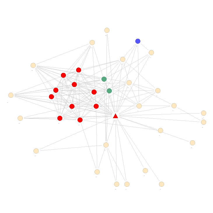
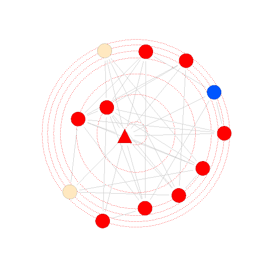
Figure 3. On the left we have the subgraphs from Tab. 5, and on the right from Tab. 6. In both cases, we first draw a Fruchterman Reingold forced drawing of the subgraph, and then a radial illustration of vertices by closeness centrality. The lowest degree vertex is denoted by a triangle. In the first case, the lowest degree vertex induces a one hop neighborhood that is much larger than the cluster, and has many low degree vertices; the vast majority (20 of 35) of these are cleaned away as singletons, marked in pale yellow. The red vertices form our cluster. The blue and green vertices belong to some other non trivial clusters. In terms of closeness centrality, vertices in the cluster are much closer to the ‘central’ (lowest degree) vertex. To the contrary, in the second cluster, the cluster is almost all of the one hop neighborhood, which has very few stray vertices. Only two of the vertices are peeled away as singletons.

As an additional experiment, we look at a citation network of computer science papers taken from a bunch of sources including DBLP, ACM, and the Microsoft Academic Graph; hosted on AMiner (Tang et al., 2008). We use version 2 from the source: this network has 660k vertices and 3M edges. Our algorithm extracted 15k non-trivial clusters. In Tab. 5, we look at an example of such a cluster: it has 11 vertices, and an edge density of 0.96. Without any information about the semantic features of the network, our algorithm is able to extract a cluster of papers on spatial joins published in similar venues such as SIGMOD, TODS and VLDB in the rough span of a decade. As another example, let us pick a sparser cluster. For this, we pick a cluster of 10 vertices with an edge density of 0.58 in Tab. 6. Here, we see a group of papers on object oriented programming focusing on traits, all from venues like TOPLAS and OOPSLA. We get thousands of such clusters, underscoring the potential for RTRExtractor for unsupervised knowledge discovery.

As an illustrative example, let us examine how these sets are extracted from our network. Recall that Alg. 1 always picks a vertex of minimal degree after passing Step 5. In both cases, the extracted sets lie entirely in the one-hop neighborhood of this lowest-degree vertex. We direct the reader to Fig. 3 (on page 12), where we provide visual descriptions of these sets. We include two images for each set: a Fruchterman-Reingold drawing (Fruchterman and Reingold, 1991), a method of forced graph drawing, and an arrangement of the same set radially by closeness centrality (Golbeck, 2013). Each image is of the immediate neighborhood of the first vertex in the network. The red vertices are the ones extracted by RTRExtractor, with the triangle being the lowest degree first vertex, and we look at the subgraph induced by this vertex and its immediate neighbors.

Our sets are formed of a tightly knit set of vertices around the lowest degree vertex: the rest are either cleaned away as singletons (marked in beige) or participate in other clusters (vertices marked in other colors). In the second case, while our subgraph is sparser, most of the neighboring vertices have a similar induced degree inside the neighborhood, and almost all of them are retained by our algorithm. In contrast, the subset in our first example is denser, but the one-hop neighborhood of the first vertex has vertices with significant variation in the induced degree. The vertices that form few (or no) triangles in the induced subgraph are all cleared away. In the closeness centrality figures, we note that the selected vertices are usually much closer to the first vertex. This is especially noticeable in the first set, where a lot of the other neighbors are peeled away as singletons.

What is excluded from the sets?

The above examples show that everything RTRExtractor includes is relevant to the set as a whole. It is natural to ask how good RTRExtractor is at not excluding relevant vertices. To examine this we look at the set of papers in the neighborhood of the first vertices that are not included in our output sets. We can confirm that this is indeed the case! This is especially true for the set in Tab. 5: of the twenty-five neighbors of the first vertex excluded from the set, only four are on spatial joins. For the set in Tab. 6, the papers are somewhat more similar (as exhibited in Fig. 3, and they all concern object hierarchies. However, the venues are significantly different, and only one of them is about traits.

8. Conclusion and Future Directions

We present the algorithm RTRExtractor and show that it succeeds at efficiently extracting sets of densely connected vertices by leveraging triangle rich-sets. Our investigation opens several doors, which we propose as future research questions.

• Cleaning: The broader principle behind the cleaning procedure in Step 5 is the removal of ‘bad’ edges with low participation in dense sets. For the extraction of dense sets, triangles are a good measure, and our proposed procedure does well. However, we believe that the idea of cleaning has rich applications as a sparsification procedure for a multitude of downstream tasks. To this end, a generalized cleaning procedure; or showing that this procedure works well for other tasks, would be a great direction for future research.

• Hierarchies: The two well-performing algorithms we compare to, the Louvain algorithm and the Nucleus algorithm, are both hierarchical clustering algorithms. This leads to the question: is there a natural setup to organize the output sets of RTRExtractor to give a hierarchy of clusters?

- (1)
- rtr (2024) 2024. https://github.com/amazon-science/amazon-RTRExtractor.
- Alsentzer et al. (2020) Emily Alsentzer, Samuel G. Finlayson, Michelle M. Li, and Marinka Zitnik. 2020. Subgraph Neural Networks. In NeurIPS 2020.
- Alvarez-hamelin et al. (2005) J. Alvarez-hamelin, Luca Dall' asta, Alain Barrat, and Alessandro Vespignani. 2005. Large scale networks fingerprinting and visualization using the k-core decomposition. In Advances in Neural Information Processing Systems, Vol. 18.
- Andersen and Chellapilla (2009) Reid Andersen and Kumar Chellapilla. 2009. Finding Dense Subgraphs with Size Bounds. In Algorithms and Models for the Web-Graph. 25–37.
- Angel et al. (2012) Albert Angel, Nikos Sarkas, Nick Koudas, and Divesh Srivastava. 2012. Dense subgraph maintenance under streaming edge weight updates for real-time story identification. Proc. VLDB Endow. 5, 6 (2012), 574–585.
- Asahiro et al. (2002) Yuichi Asahiro, Refael Hassin, and Kazuo Iwama. 2002. Complexity of finding dense subgraphs. Discrete Applied Mathematics 121, 1 (2002), 15–26.
- Bansal et al. (2004) Nikhil Bansal, Avrim Blum, and Shuchi Chawla. 2004. Correlation Clustering. Machine Learning 56, 1 (01 Jul 2004), 89–113.
- Basu et al. (2023) Sabyasachi Basu, Suman K. Bera, and C. Seshadhri. 2023. A spectral theorem on the cluster structure of real world graphs. https://tr.soe.ucsc.edu/research/technical-reports/UCSC-SOE-23-09
- Beal et al. (2003) Daniel Judson Beal, Robin R. Cohen, Michael J. Burke, and Christy L McLendon. 2003. Cohesion and performance in groups: a meta-analytic clarification of construct relations. The Journal of applied psychology 88 6 (2003), 989–1004.
- Benson et al. (2016) A. Benson, D. F. Gleich, and J. Leskovec. 2016. Higher-order organization of complex networks. Science 353, 6295 (2016), 163–166.
- Blondel et al. (2008) Vincent D Blondel, Jean-Loup Guillaume, Renaud Lambiotte, and Etienne Lefebvre. 2008. Fast unfolding of communities in large networks. Journal of Statistical Mechanics: Theory and Experiment 2008, 10 (oct 2008), P10008.
- Bonchi et al. (2021) Francesco Bonchi, David García-Soriano, Atsushi Miyauchi, and Charalampos E. Tsourakakis. 2021. Finding densest -connected subgraphs. Discrete Applied Mathematics 305 (Dec. 2021), 34–47.
- Boob et al. (2020) Digvijay Boob, Yu Gao, Richard Peng, Saurabh Sawlani, Charalampos Tsourakakis, Di Wang, and Junxing Wang. 2020. Flowless: Extracting Densest Subgraphs Without Flow Computations. In Proceedings of The Web Conference 2020 (WWW ’20). Association for Computing Machinery, 573–583.
- Buehrer and Chellapilla (2008) Gregory Buehrer and Kumar Chellapilla. 2008. A scalable pattern mining approach to web graph compression with communities (WSDM ’08). 95–106.
- Charikar (2000) Moses Charikar. 2000. Greedy Approximation Algorithms for Finding Dense Components in a Graph. In Approximation Algorithms for Combinatorial Optimization. 84–95.
- Chekuri et al. ([n.d.]) Chandra Chekuri, Kent Quanrud, and Manuel R. Torres. [n.d.]. Densest Subgraph: Supermodularity, Iterative Peeling, and Flow. 1531–1555.
- Chen and Saad (2012) Jie Chen and Yousef Saad. 2012. Dense Subgraph Extraction with Application to Community Detection. IEEE Transactions on Knowledge and Data Engineering 24, 7 (2012), 1216–1230.
- Chiba and Nishizeki (1985) Norishige Chiba and Takao Nishizeki. 1985. Arboricity and Subgraph Listing Algorithms. SIAM J. Comput. 14, 1 (1985), 210–223.
- Cohen (2008) J. Cohen. 2008. Trusses: Cohesive subgraphs for social network analysis. In Technical report, National Security Agency.
- Danisch et al. (2017) Maximilien Danisch, T.-H. Hubert Chan, and Mauro Sozio. 2017. Large Scale Density-friendly Graph Decomposition via Convex Programming (WWW ’17). 233–242.
- Dourisboure et al. (2007) Yon Dourisboure, Filippo Geraci, and Marco Pellegrini. 2007. Extraction and classification of dense communities in the web. In Proceedings of the 16th International Conference on World Wide Web (WWW ’07). 461–470.
- Du et al. (2009) Xiaoxi Du, Ruoming Jin, Liang Ding, Victor E. Lee, and John H. Thornton. 2009. Migration motif: a spatial - temporal pattern mining approach for financial markets. In Proceedings of the 15th ACM SIGKDD International Conference on Knowledge Discovery and Data Mining (KDD ’09). 1135–1144.
- Fang et al. (2020) Yixiang Fang, Xin Huang, Lu Qin, Ying Zhang, Wenjie Zhang, Reynold Cheng, and Xuemin Lin. 2020. A survey of community search over big graphs. The VLDB Journal 29, 1 (2020), 353–392.
- Feige (2002) Uriel Feige. 2002. Relations between average case complexity and approximation complexity (STOC ’02). 534–543.
- Forsyth (2010) D.R. Forsyth. 2010. Group Dynamics. Wadsworth.
- Frasca et al. (2022) Fabrizio Frasca, Beatrice Bevilacqua, Michael M. Bronstein, and Haggai Maron. 2022. Understanding and Extending Subgraph GNNs by Rethinking Their Symmetries. arXiv:2206.11140 [cs.LG]
- Fratkin et al. (2006) Eugene Fratkin, Brian T Naughton, Douglas L Brutlag, and Serafim Batzoglou. 2006. MotifCut: regulatory motifs finding with maximum density subgraphs. Bioinformatics (Oxford, England) 22, 14 (2006), e150—7.
- Fruchterman and Reingold (1991) Thomas M. J. Fruchterman and Edward M. Reingold. 1991. Graph drawing by force-directed placement. Software: Practice and Experience 21, 11 (1991), 1129–1164.
- Gibson et al. (2005) David Gibson, Ravi Kumar, and Andrew Tomkins. 2005. Discovering large dense subgraphs in massive graphs. In Proceedings of the 31st International Conference on Very Large Data Bases (VLDB ’05). 721–732.
- Gionis et al. (2013) Aristides Gionis, Flavio Junqueira, Vincent Leroy, Marco Serafini, and Ingmar Weber. 2013. Piggybacking on social networks. Proc. VLDB Endow. 6, 6 (2013), 409–420.
- Girvan and Newman (2002) M. Girvan and M. Newman. 2002. Community structure in social and biological networks. Proceedings of the National Academy of Sciences 99, 12 (2002), 7821–7826.
- Golbeck (2013) Jennifer Golbeck. 2013. Chapter 3 - Network Structure and Measures. In Analyzing the Social Web. 25–44.
- Goldberg (1984) A. V. Goldberg. 1984. Finding a Maximum Density Subgraph. Technical Report. USA.
- Gupta et al. (2014) Rishi Gupta, Tim Roughgarden, and C. Seshadhri. 2014. Decompositions of Triangle-Dense Graphs. Innovations in Theoretical Computer Science (2014), 471–482.
- Håstad (1999) Johan Håstad. 1999. Clique is hard to approximate within 1-. Acta Mathematica 182, 1 (01 Mar 1999), 105–142.
- Huang and Lakshmanan (2017) Xin Huang and Laks V. S. Lakshmanan. 2017. Attribute-driven community search. Proceedings of the VLDB Endowment 10, 9 (2017), 949–960.
- Iasemidis et al. (2003) Leonidas D. Iasemidis, Deng-Shan Shiau, Wanpracha Art Chaovalitwongse, J. Chris Sackellares, Panos M. Pardalos, José C. Príncipe, Paul R. Carney, Awadhesh Prasad, Balaji Veeramani, and Kostas Tsakalis. 2003. Adaptive epileptic seizure prediction system. IEEE Trans. Biomed. Eng. 50, 5 (2003), 616–627.
- Jin et al. (2021) Di Jin, Zhizhi Yu, Pengfei Jiao, Shirui Pan, Dongxiao He, Jia Wu, Philip Yu, and Weixiong Zhang. 2021. A Survey of Community Detection Approaches: From Statistical Modeling to Deep Learning. IEEE Transactions on Knowledge and Data Engineering (2021), 1–1.
- Jin et al. (2009) Ruoming Jin, Yang Xiang, Ning Ruan, and David Fuhry. 2009. 3-HOP: a high-compression indexing scheme for reachability query. In Proceedings of the 2009 ACM SIGMOD International Conference on Management of Data (SIGMOD ’09). 813–826.
- Khot (2006) Subhash Khot. 2006. Ruling Out PTAS for Graph Min-Bisection, Dense k-Subgraph, and Bipartite Clique. SIAM J. Comput. 36, 4 (2006), 1025–1071.
- Konar and Sidiropoulos (2022) Aritra Konar and Nicholas D. Sidiropoulos. 2022. The Triangle-Densest-K-Subgraph Problem: Hardness, Lovász Extension, and Application to Document Summarization. Proceedings of the AAAI Conference on Artificial Intelligence 36, 4 (Jun. 2022), 4075–4082.
- Kumar et al. (1999) Ravi Kumar, Prabhakar Raghavan, Sridhar Rajagopalan, and Andrew Tomkins. 1999. Trawling the Web for emerging cyber-communities. Computer Networks 31, 11 (1999), 1481–1493.
- Lanciano et al. (2023) Tommaso Lanciano, Atsushi Miyauchi, Adriano Fazzone, and Francesco Bonchi. 2023. A Survey on the Densest Subgraph Problem and its Variants. arXiv:2303.14467 [cs.DS]
- Lee et al. (2010) Victor E. Lee, Ning Ruan, Ruoming Jin, and Charu Aggarwal. 2010. A Survey of Algorithms for Dense Subgraph Discovery. Springer US, 303–336.
- Leskovec and Krevl (2014) Jure Leskovec and Andrej Krevl. 2014. SNAP Datasets: Stanford Large Network Dataset Collection. http://snap.stanford.edu/data.
- Leskovec et al. (2008) Jure Leskovec, Kevin J. Lang, Anirban Dasgupta, and Michael W. Mahoney. 2008. Statistical Properties of Community Structure in Large Social and Information Networks. In Proceedings of the 17th International Conference on World Wide Web (WWW ’08). 695–704.
- Matula and Beck (1983) David W. Matula and Leland L. Beck. 1983. Smallest-last ordering and clustering and graph coloring algorithms. J. ACM 30, 3 (jul 1983), 417–427. https://doi.org/10.1145/2402.322385
- Miyauchi and Kakimura (2018) Atsushi Miyauchi and Naonori Kakimura. 2018. Finding a Dense Subgraph with Sparse Cut (CIKM ’18). 547–556.
- Miyauchi and Kawase (2015) Atsushi Miyauchi and Yasushi Kawase. 2015. What Is a Network Community? A Novel Quality Function and Detection Algorithms (CIKM ’15). 1471–1480.
- Raghavan et al. (2007) Usha Nandini Raghavan, Réka Albert, and Soundar Kumara. 2007. Near linear time algorithm to detect community structures in large-scale networks. Phys. Rev. E 76 (Sep 2007), 036106. Issue 3.
- Rosvall et al. (2009) M. Rosvall, D. Axelsson, and C. T. Bergstrom. 2009. The map equation. The European Physical Journal Special Topics 178, 1 (Nov. 2009), 13–23.
- Rosvall and Bergstrom (2008) Martin Rosvall and Carl T. Bergstrom. 2008. Maps of random walks on complex networks reveal community structure. Proceedings of the National Academy of Sciences 105, 4 (2008), 1118–1123.
- Sariyuce et al. (2015) A. Erdem Sariyuce, C. Seshadhri, A. Pinar, and U. Catalyurek. 2015. Finding the Hierarchy of Dense Subgraphs using Nucleus Decompositions. In World Wide Web (WWW). 927–937.
- Satuluri et al. ([n.d.]) Venu Satuluri, Srinivasan Parthasarathy, and Yiye Ruan. [n.d.]. Local graph sparsification for scalable clustering (SIGMOD ’11). 721–732.
- Schank and Wagner (2005) Thomas Schank and Dorothea Wagner. 2005. Finding, Counting and Listing All Triangles in Large Graphs, an Experimental Study. In Experimental and Efficient Algorithms. Springer Berlin / Heidelberg, 606–609.
- Seshadhri (2023) C. Seshadhri. 2023. Some Vignettes on Subgraph Counting Using Graph Orientations. In International Conference on Database Theory (ICDT 2023), Vol. 255. 3:1–3:10.
- Shin et al. (2016) Kijung Shin, Tina Eliassi-Rad, and Christos Faloutsos. 2016. CoreScope: Graph Mining Using k-Core Analysis — Patterns, Anomalies and Algorithms (ICDM ’16). 469–478.
- Sotirov (2020) Renata Sotirov. 2020. On solving the densest k-subgraph problem on large graphs. Optimization Methods and Software 35, 6 (2020), 1160–1178.
- Tang et al. (2008) Jie Tang, Jing Zhang, Limin Yao, Juanzi Li, Li Zhang, and Zhong Su. 2008. ArnetMiner: Extraction and Mining of Academic Social Networks. SIGKDD Conference on Knowledge Discovery and Data Mining (KDD) (2008), 990–998.
- Traag et al. (2019) V.A. Traag, L. Waltman, and N.J. van Eck. 2019. From Louvain to Leiden: guaranteeing well-connected communities. Scientific Reports 9, 5233 (2019).
- Tsourakakis (2014) Charalampos E. Tsourakakis. 2014. A Novel Approach to Finding Near-Cliques: The Triangle-Densest Subgraph Problem. CoRR abs/1405.1477 (2014).
- Tsourakakis (2015) Charalampos E. Tsourakakis. 2015. The K-clique Densest Subgraph Problem. In Proceedings of the 24th International Conference on World Wide Web. 1122–1132.
- Tsourakakis et al. ([n.d.]) Charalampos E. Tsourakakis, Jakub Pachocki, and Michael Mitzenmacher. [n.d.]. Scalable Motif-aware Graph Clustering (WWW ’17). 1451–1460.
- Veldt et al. ([n.d.]) Nate Veldt, David F. Gleich, and Anthony Wirth. [n.d.]. A Correlation Clustering Framework for Community Detection (WWW ’18). 439–448.
- Wang and Cheng (2012) Jia Wang and James Cheng. 2012. Truss decomposition in massive networks. Proc. VLDB Endow. 5, 9 (2012), 812–823.
- Wang et al. (2010) Nan Wang, Jingbo Zhang, Kian-Lee Tan, and Anthony K. H. Tung. 2010. On triangulation-based dense neighborhood graph discovery. Proc. VLDB Endow. 4, 2 (2010), 58–68.
- Xu et al. (2023) Yichen Xu, Chenhao Ma, Yixiang Fang, and Zhifeng Bao. 2023. Efficient and Effective Algorithms for Generalized Densest Subgraph Discovery. Proc. ACM Manag. Data 1, 2, Article 169 (2023).
- Zhang and Horvath (2005) Bin Zhang and Steve Horvath. 2005. A general framework for weighted gene co-expression network analysis. Statistical applications in genetics and molecular biology 4 (2005), Article17.