Automated modal analysis of entanglement with bipartite self-configuring optics

Abstract

Entanglement is a unique feature of quantum mechanics. In coupled systems of light and matter, entanglement manifests itself in the linear superposition of multipartite quantum states (e.g., parametrized by the multiple spatial, spectral, or temporal degrees of freedom of a light field). In bipartite systems, the Schmidt decomposition provides a modal decomposition of the entanglement structure over independent, separable states. Although ubiquitous as a tool to describe and measure entanglement, there exists no general method to decompose a bipartite quantum state onto its Schmidt modes. Here, we propose a method that relies on bipartite self-configuring optics that automatically “learns” the Schmidt decomposition of an arbitrary pure quantum state. Our method is agnostic to the degrees of freedom over which quantum entanglement is distributed and can reconstruct the Schmidt modes and values by variational optimization of the network’s output powers or coincidences. We illustrate our method with numerical examples of spectral entanglement analysis for biphotons generated via spontaneous parametric down conversion and provide experimental guidelines for its realization, including the influence of losses and impurities. Our method provides a versatile and scalable way of analyzing entanglement in bipartite integrated quantum photonic systems.

Entanglement is a fundamental property of quantum mechanical systems horodecki2009quantum , underpinning quantum computing algorithms shor1999polynomial , cryptography yin2020entanglement , teleportation protocols bouwmeester1997experimental , and tests of non-local realism aspect1982experimental ; groblacher2007experimental . Optics is a prime platform for the generation and manipulation of entanglement between the many degrees of freedom of light and matter systems raimond2001manipulating ; o2009photonic ; wineland2013nobel ; erhard2020advances . A paradigmatic example of bipartite entangled states in optics are photon pairs generated via spontaneous parametric down conversion (SPDC), which have been the workhorse of quantum photonic logic, computing, and simulations carolan2015universal ; zhong2020quantum ; bogdanov2004qutrit ; zhang2024entanglement . There has been a growing interest in controlling entanglement of photon pairs with engineered pumps and nonlinear crystals burlakov1999polarization ; fedorov2008spontaneous ; fedorov2011entanglement ; hurvitz2023frequency ; shukhin2024two . Such engineered quantum sources may be used to shape separable biphoton wavefunctions for heralding dosseva2016shaping ; meyer2017limits ; graffitti2018design and for quantum information processing graffitti2020direct ; morrison2022frequency ; shukhin2024two .

A successful implementation of quantum computing and simulation protocols entails an accurate description and characterization of entanglement. In pure bipartite quantum systems, measures of entanglement are provided by the Schmidt number and the von Neumann entropy horodecki2009quantum . Generally, the Schmidt decomposition of a pure bipartite state provides a convenient modal description of entanglement (as a linear superposition of separable and orthogonal “Schmidt modes”) fedorov2014schmidt ; sharapova2015schmidt . When the Hilbert space of photon pairs is low-dimensional, the quantum state and its underlying entanglement can be unveiled with a finite set of projective measurements toninelli2019concepts . However, when the Hilbert space becomes large and even continuous, as in the case of spatial and spectral correlations just2013transverse ; sharapova2015schmidt ; graffitti2020direct ; morrison2022frequency ; shukhin2024two , methods to experimentally measure the Schmidt modes are more challenging to implement. Such methods have been implemented for photon pairs with a priori knowledge of the mode shape straupe2011angular . Despite the ubiquity and usefulness of Schmidt modes in describing multimode entanglement, there is no general method to experimentally determine the Schmidt decomposition of a pure biphoton state.

Programmable networks of Mach-Zehnder interferometers (MZIs) bogaerts_programmable_2020 ; harris2018linear are an ideal platform for integrated quantum photonics o2009photonic . They have enabled the realization of quantum key distribution sibson2017chip , variational quantum algorithms peruzzo2014variational ; carolan2020variational , multidimensional and multiphoton entanglement processing matthews2009manipulation ; wang2018multidimensional , and quantum walk simulators harris2017quantum . In these demonstrations, the enabling feature of programmable MZI networks is that they can impart arbitrary unitary operators on spatial modes of quantum optical states miller2013self ; miller2013self2 ; carolan2015universal .

Self-configuring programmable network architectures miller2013self ; miller2013self2 ; miller2019waves ; seyedinnavadeh_determining_2023 ; MillerAnalyze2020 ; milanizadeh2021coherent ; pai2023experimentally ; miller2015perfect ; miller2013establishing ; roques2024measuring additionally offer simple and progressive configuration of the MZIs based only on power minimizations or maximizations, adapting automatically to the problem of interest, sometimes even without calculations. They can learn modal representations of (quantum) optical fields (e.g., communication modes miller2013establishing ; miller2019waves ; seyedinnavadeh_determining_2023 and natural modes of partially coherent light roques2024measuring ). However, their potential in the modal analysis of entanglement in bipartite quantum optical systems has not been explored thus far.

Here, we propose a general method to automatically analyze entanglement in bipartite quantum optical systems using self-configuring optics. Our approach relies on bipartite self-configuring networks (BSCN) composed of MZI meshes that impart unitary transformations to the two subspaces of the bipartite system. The average power or coincidence counts at the output of the BSCN are sequentially optimized, which results in the network having “learned” the Schmidt decomposition of an input state. Then, the Schmidt number can be directly measured at the output (as the number of ports with non-zero average power/coincidence), and the Schmidt modes of the system can be deduced directly from the network’s settings. Our approach thus automatically discovers the Schmidt modes without presuming any prior knowledge about these modes.

We illustrate our method with numerical examples of photon pairs generated via SPDC in various phase-matching settings. We show that our method can automatically measure Schmidt modes of photon pairs while being robust to single photon losses. Since our method allows us to automatically learn a modal decomposition of entanglement in the system, we also discuss potential applications in modal shaping of separable light and generation of states with controlled entanglement. Our method paves the way to full characterization, processing, and generation of entanglement in quantum optical states in a robust, scalable, and tunable manner. We envision that our approach could form a building block in integrated quantum optical architectures for computing and simulation where entanglement measurement and control plays an essential role.

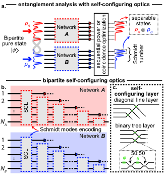
Figure 1: Automatic Schmidt decomposition of bipartite quantum optical systems with self-configuring optics. a. Conceptual schematic of automatic Schmidt decomposition enabled by bipartite self-configuring optics. A bipartite pure state $\ket{\psi_{\text{in}}}$ is input to two networks $A$ and $B$ acting upon Hilbert spaces $H_{A}$ and $H_{B}$, respectively. Their outputs (either power or coincidence counts) are sequentially optimized. The resulting output is a linear superposition of orthogonal separable states (Schmidt decomposition), and the Schmidt number can be read off as the number of non-zero outputs. b. Bipartite self-configuring network (BSCN) architecture. Each network consists of a cascade of self-configuring layers (SCLs). Each such SCL separates one mode to its output port (here, the top one in each layer), passing the remaining field to the next layer. c. SCL architecture, consisting of, e.g., a diagonal line or binary tree layer MillerAnalyze2020 . Each node corresponds to a 2 by 2 Mach-Zehnder interferometer (MZI) parametrized by phases $(\varphi,\theta)$.

Automatic Schmidt decomposition and entanglement analysis of bipartite quantum optical systems with self-configuring optics

We consider a pure state input $\ket{\psi_{\text{in}}}$ to the BSCN of Figure 1 (later, we shall consider photonic losses that might impair the state’s purity). The input state is bipartite and is defined over the tensor product of two Hilbert spaces $H_{A}$ and $H_{B}$, with dimensions $N_{A}$ and $N_{B}$, respectively. These dimensions can be large, and even cover the (discretized) case of a continuous Hilbert space, e.g., as in spectral-bin encoding morrison2022frequency ; lu2023frequency . A concrete example of this model consists of two single photons propagating over spatial modes of integrated networks $A$ (red) and $B$ (blue). We can decompose the state over an orthogonal basis $\ket{x_{j}}_{A}\ket{x_{k}}_{B}$ of $H_{A}\otimes H_{B}$ and write its Schmidt decomposition as:

$$\ket{\psi_{\text{in}}} =\sum_{jk}G_{jk}\ket{x_{j}}_{A}\ket{x_{k}}_{B}$$ (1)

$$=\sum_{i=1}^{r}\lambda_{i}\ket{y_{i}}_{A}\ket{y_{i}}_{B},$$ (2)

where $G$ is a $N_{A}\times N_{B}$ state matrix whose singular value decomposition $G=UDV^{\dagger}$ maps to the input state’s Schmidt decomposition nielsen2010quantum as $\ket{y_{i}}_{A}=\sum_{j}U_{ji}\ket{x_{j}}_{A}$, $\ket{y_{i}}_{B}=\sum_{j}V^{*}_{ki}\ket{x_{k}}_{B}$, and $D_{ii}=\lambda_{i}$ are the $r$ singular values of $G$ (ordered by decreasing value $\lambda_{1}\geq\ldots\geq\lambda_{r}>0)$. As can be seen from Equation (2), the Schmidt decomposition provides a modal description of entanglement as a linear superposition of mutually orthogonal and separable states. The Schmidt number $r$, which quantifies the amount of entanglement in the state, corresponds to the number of non-zero $\lambda_{i}$’s. The Schmidt decomposition directly yields the von Neumann entropy of the input state: $S=-\sum_{k}\lambda_{k}^{2}\log(\lambda_{k}^{2})$.

The network shown in Figure 1 can automatically perform Schmidt decomposition of an input state $\ket{\psi_{\text{in}}}$ by simultaneous diagonalization of the reduced density operators of each subspace. The network is made of two cascades of self-configuring layers (SCLs) that form networks $A$ and $B$ (see Figure 1(b)). SCL architectures can be defined topologically  MillerAnalyze2020 ; each SCL has a single output that is connected to each input by only one path through the MZI blocks .

These SCL cascades operate on spaces $H_{A}$ and $H_{B}$, respectively, transforming their reduced density matrices as $\rho^{A}\rightarrow U^{A}\rho^{A}(U^{A})^{\dagger}$ and $\rho^{B}\rightarrow U^{B}\rho^{B}(U^{B})^{\dagger}$ where $U^{A}$ and $U^{B}$ are reconfigurable unitary matrices imparted by networks $A$ and $B$, respectively. This SCL architecture allows for the implementation of sequential, layer-by-layer optimization methods miller2013self ; miller2013self2 ; roques2024measuring . Example SCL architectures include diagonal lines or binary trees of MZIs MillerAnalyze2020 , as shown in Figure 1(c). These sequential, layer-by-layer optimizations over parameters of the BSCN can be realized by dithering milanizadeh2021coherent ; seyedinnavadeh_determining_2023 or in situ back-propagation hughes2018training ; pai2023experimentally .

We now show how the BSCN of Figure 1 can learn the Schmidt decomposition of the input state $\ket{\psi_{\text{in}}}$. Sequential optimization of the average output powers measured at port $k$ $\braket{P^{A}_{k}}$ ($k=1,\ldots,N_{A}$) and $\braket{P^{B}_{k}}$ ($k=1,\ldots,N_{B}$) maps to a variational definition of the eigendecomposition of $GG^{\dagger}$ and $(G^{\dagger}G)^{T}$ (see Supplementary Materials (SM), Sections S1 and S2):

$$\underset{\tau^{A}_{k}}{\text{max}}\braket{P^{A}_{k}} =\underset{u_{k}^{A}}{\text{max}}~{}(u_{k}^{A})^{\dagger}(GG^{\dagger})u_{k}^{A}=\lambda_{k}^{2},$$ (3)

$$\underset{\tau^{B}_{k}}{\text{max}}\braket{P^{B}_{k}} =\underset{u_{k}^{B}}{\text{max}}~{}(u_{k}^{B})^{\dagger}(G^{\dagger}G)^{T}u_{k}^{B}=\lambda_{k}^{2},$$ (4)

where $\tau^{A}_{k}$ (resp., $\tau^{B}_{k}$) are the parameters of the $k$-th self-configuring layer of network $A$ (resp., $B$), and $u_{k}^{A}$ (resp. $u_{k}^{B}$) the $k$-th column of $(U^{A})^{\dagger}$ (resp., $(U^{B})^{T}$). One can see from Equations (3, 4) that tracing out subspace $B$ (resp., $A$) allows for the variational definition of the left (resp., right) singular vectors of $G$ and their respective singular values.

Alternatively, sequential optimization of the single-photon coincidence counts between output ports $k$ of networks $A$ and $B$ (where $k=1,\ldots,\text{min}(N_{A},N_{B})$) directly maps to a singular value decomposition of $G$ (see SM, Section S2):

$$\underset{\tau^{A}_{k},\tau^{B}_{k}}{\text{max}}\braket{C_{kk}}=\underset{u_{k}^{A},u_{k}^{B}}{\text{max}}|(u^{A}_{k})^{\dagger}Gu^{B}_{k}|^{2}=\lambda_{k}^{2},$$ (5)

where the optimization runs over the $k$-th self-configuring layers of $A$ and $B$ simultaneously. Both optimization methods will result in setting the network parameters to that of the Schmidt modes, corresponding to the singular value decomposition of $G$, such that $U^{A}=U^{\dagger}$ and $U^{B}=V^{T}$.

Both sequential optimization methods provide an automatic way to find the Schmidt decomposition of the input state $\ket{\psi_{\text{in}}}$. The resulting settings of the BSCN allow one to “read” the Schmidt modes (corresponding, for instance, to the decomposition of the complex joint spectral amplitude (JSA) of a biphoton state), and the Schmidt number corresponds to half the number of output ports with non-zero average power, or the number of output port pairs of same index with non-zero coincidence. When considering two output ports sharing the same index $k$, $\ket{x_{k}}_{A}\ket{x_{k}}_{B}$, their joint output state is separable and corresponds to the amplitude of the Schmidt mode with singular value $\lambda_{k}$. Individual Schmidt modes can be physically generated by feeding their corresponding output ports (while blocking the rest) as inputs to a pair of complementary networks applying $U_{A}^{\dagger}$ and $U_{B}^{\dagger}$ (as shown in Figure 4). A detailed derivation and description of the sequential optimization methods can be found in the SM, Sections S1 and S2.

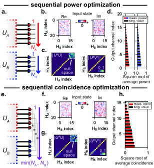
Figure 2: Sequential optimization methods for entanglement analysis in self-configuring optics. a-d. Sequential power optimization. a. Power optimization sequence: from $1$ to $N_{A}$ (on outputs of network $A$), then from $1$ to $N_{B}$ (on outputs of network $B$). b. Random matrix input example. c. Resulting eigenvector reconstruction from power optimization. d. Resulting simulated square roots of power outputs (meas. power) and singular values (sing. values) at the outputs of network $A$ (red) and $B$ (blue). e-h. Sequential coincidence counts optimization. e. Coincidence counts optimization sequence: from $1$ to $\text{min}(N_{A},N_{B})$ (on pairs of outputs ports from networks $A$ and $B$). f. Random matrix input example. g. Resulting eigenvector reconstruction from coincidence optimization. h. Resulting simulated square roots of coincidence counts (meas. coinc.) and singular values (sing. values).

In the following, we turn to numerical examples illustrating our method, first with random matrices, to show the generality of this approach, and then the experimentally-relevant case of photon pairs generated via SPDC.

In this first numerical example, we consider the performance of the two sequential optimization methods mentioned in the previous section. In both cases, gradients are calculated via automatic differentiation and optimization is performed via stochastic gradient descent kingma2014adam . The power optimization method (Figure 2(a)) runs over output ports $k$ of network $A$ for $k=1,\ldots,N_{A}$ and then $k$ of network $B$ for $k=1,\ldots,N_{B}$. We simulate the performance of the sequential power optimization over the outputs of the BSCN on a random matrix (shown in Figure 2(b)). First, the network learns the singular vectors of the state matrix $G$: this can be seen by plotting $U^{A}U$ and $U^{B}V^{*}$, which are equal to the identity matrix (except on the null space, see Figure 2(c)). The corresponding singular values can be read as the square root of the average power on the output ports of networks $A$ and $B$, as shown in Figure 2(d). The performance of the sequential coincidence maximization is shown on a similar random matrix $G$ in Figure 2(e-h), where similar performance is achieved, and the singular values can be measured as the square root of the average coincidence between ports $\ket{x_{k}}_{A}$ and $\ket{x_{k}}_{B}$. In these examples, the BSCN accurately identifies the Schmidt modes and values.

If single photons in either subspace are lost (e.g., absorbed or scattered), the output mixes with the vacuum state, which might result in errors in the average power measured. We show in the SM, Section S3 that, when modeling detection or scattering losses as coupling each output waveguide to a reservoir, the influence of losses can be calibrated out by measuring the average power transmission at each output port. Large losses may however result in reducing the number of counts on the detector and slow down the training process. Other MZI mesh architectures may also alleviate the influence of losses and imperfections burgwal2017using ; miller2015perfect . This intrinsic robustness to single photon losses provides further motivation to investigate the performance of our method in experimentally-relevant settings.

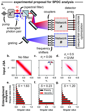
Figure 3: Automatic entanglement analysis of spontaneous parametric down-converted (SPDC) photons. a. Proposed experimental setup to automatically analyze entanglement of photon pairs generated via non-degenerate SPDC. A laser at frequency $\omega_{p}$ is pumping a second-order nonlinear crystal spontaneously generating entangled photon pairs at idler and signal frequencies $(\omega_{i},\omega_{s})$, separated by a polarization beam splitter (PBS). Different frequency components are routed to different input ports of two self-configuring networks (SCN) denoted $A$ ($\omega_{i}$) and $B$ ($\omega_{s}$). The SCN perform sequential coincidence counts maximization to automatically perform the Schmidt decomposition of the photon pair. b-d. Input joint spectral amplitude (JSA). e-g. Entanglement analysis with BSCN. $S$ denotes the von Neumann entropy. b, e. Numerical results for an unfiltered SPDC experiment ($\sigma_{f}\rightarrow\infty$, as defined in SM, Section S4). c, f. Same as b, e., but with a filter applied to the signal and idler modes ($\sigma_{f}=0.09$). d, g. Same as b, e., but with a filter ($\sigma_{f}=0.2$) and group velocity mismatch (GVM) corrections. All frequencies are normalized to frequency range of interest: pump bandwidth is $\sigma=0.1$ for (b-c.) and $\sigma=0.5$ for (d.).

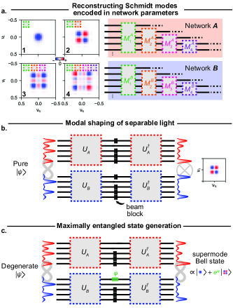
Figure 4: Schmidt mode reconstruction and entangled light processing with bipartite self-configuring optics. a. Left: First four Schmidt modes reconstructed from BSCN parameters in the SPDC example of Figure 3d,g.. Right: BSCN architecture for reference, where each self-configuring layer is highlighted in a different color. The self-configuring layers used to reconstruct the Schmidt modes on the left are represented by the number and color of gray squares as insets. b. Once trained, BSCN can be used to generate separable light with of a given modal shape by blocking all output ports except the two ports corresponding to that mode index (in networks $A$ and $B$) and feeding them as input to networks applying the inverse transformation. c. If trained on a highly degenerate input state (such that two singular values are approximately equal), BSCN can also be used to generate supermode Bell states (by blocking all output ports except the four ports corresponding to degenerate singular values in each network). An additional phase shifter can be added on one of the output ports to control the relative phase between the two terms of the pair.

Analyzing and processing entanglement in spontaneously down-converted photon pairs

We now investigate the performance of our method in the analysis of entangled photon pairs generated via SPDC. As noted in the previous section, our method is naturally suited for the analysis of spatial mode entanglement. To further generalize the applicability of our approach, we consider below the case of frequency bin entanglement. This concept could be readily generalized to other high-dimensional Hilbert spaces, e.g., correlations in spatial modes such as orbital angular momentum mair2001entanglement ; erhard2018twisted ; kovlakov2018quantum . The proposed experimental setup that we model is shown in Figure 3(a). We consider a second-order nonlinear crystal pumped by a laser at frequency $\omega_{p}$ and spontaneously generating photon pairs at frequencies $\omega_{s}$ (signal) and $\omega_{i}$ (idler). The SPDC photons then go through an optional spectral filter to shape the joint spectral density (width $\sigma_{f}$) and a polarizing beam splitter to split signal and idler beams. Gratings are then used to diffract spectral modes of the idler (signal) photons, occupying equidistant frequency bins centered around $\omega_{i(s),j}=\omega_{i(s),0}+j\Omega$, into corresponding spatial input modes $x_{j}$ (which couple to the network with a grating coupler). The frequency bins, now occupying different spatial modes, are then shifted to a common frequency $\omega_{i(s),0}$ (see SM section S5). This can be done by an array of (on-chip) electro-optic frequency shifters hu2021chip ; zhu2022spectral ; lingaraju2022bell ; lu2023frequency driven by corresponding $\Omega$ harmonics .

In the absence of losses and spectral mixing by the gratings, the resulting input state to the BSCN is:

$$\ket{\psi_{\text{in}}}=\sum_{j,k}f(\nu_{s,j},\nu_{i,k})\ket{x_{j}}_{A}\ket{x_{k}}_{B},$$ (6)

where $f(\nu_{s},\nu_{i})$ is the JSA of the photon pair at frequency $(\nu_{s},\nu_{i})$, and $\nu_{s,j}=\omega_{s,j}-\omega_{s,0}$ and $\nu_{i,k}=\omega_{i,k}-\omega_{i,0}$ correspond to the discrete frequency bins around the central frequencies. The JSA can be controlled by shaping the incident pump spectrum werner1995ultrashort ; arzani2018versatile , the nonlinear crystal poling pattern graffitti2020direct ; morrison2022frequency ; shukhin2024two , via dispersion engineering u2006generation ; CHRIST2013351 , or adiabatic frequency conversion presutti2024highly . Below, we shall focus on the ubiquitous scenarios of spectral filtering and group velocity mismatch between the pump, signal, and idler (Figure 3(d,g)). Further details on our experimental model can be found in SM, Section S4.

Several phase-matching settings are shown in Figures 3(b-d), as well as the BSCN output after convergence in Figures 3(e-g). In all cases, the BSCN learns the Schmidt decomposition of the input state, and we can use the average coincidence counts to calculate the input state’s von Neumann entropy (with negligible error compared to ground truth value $<1\%$). The addition of a spectral filter in Figure 3(c,f) reduces the entanglement by removing spectral components of the photon pair, namely making the state “more separable.” In general, group velocity mismatch is present (Figure 3(d,g)), resulting in anti-correlated side lobes in the JSA. Several methods have been proposed to further shape the joint spectral density with engineered crystals hurvitz2023frequency and pumps boucher2021engineering and the BSCN could be also applied to perform modal analysis of entanglement in these cases as well. We note that the experimental proposal from Figure 3 might be generalized to a fully integrated setup. This could be achieved by leveraging on-chip biphoton sources luo2017chip ; chapman2024chip and would avoid coupling losses due to grating couplers.

A distinctive feature of our method is that the Schmidt modes (including their phases) are directly encoded into the parameters of the network after it has converged. Specifically, the $k$-th Schmidt mode is encoded in the network parameters (e.g., the phase shifts for various waveguide segments of MZIs) of layers $1,\ldots,k$ of both networks $A$ and $B$. We can therefore reconstruct the Schmidt modes (of the SPDC example from Figure 3(d)) as shown in Figure 4(a). The self-configuring layers used for the reconstruction of each mode are indicated with dashed square boxes in each panel.

By automatically performing modal decomposition of the entanglement structure of the input state, the BSCN offers other possibilities in modal shaping and generation of entanglement states. Namely, by blocking all output ports except the ones corresponding to a given biphoton mode, and using them as inputs for a pair of inverse networks (or even by reflecting them back through the output ports of the original networks), one can generate separable states with known shape (e.g., in spectral or spatial domain), as shown in Figure 4(b). Additionally, if one inputs a degenerate quantum state (such that $\lambda_{1}\approx\lambda_{2}$, as can be done with broadband phase-matching zielnicki2018joint or engineered nonlinear crystals hurvitz2023frequency ), a “supermode Bell state” can be generated by considering the output of the first two ports of both networks: $\ket{\psi_{\text{out}}}\propto\lambda_{1}(\ket{x_{1}}_{A}\ket{x_{1}}_{B}+e^{i\varphi}\ket{x_{2}}_{A}\ket{x_{2}}_{B})$, where an additional phase $\varphi$ can be imparted by a phase shifter on one of the output ports.

Discussion

We further discuss potential applications of our method and experimental considerations for their realization.

Our methods could be applied to entanglement analysis in other quantum systems, such as temporal entanglement in atom-photon coupling bogdanov2006schmidt and macroscopic quantum states of light, such as bright squeezed vacuum sharapova2015schmidt ; sharapova2018bright . In both cases, multimodal entanglement over temporal, spatial, or spectral degrees of freedom can be described on the Schmidt basis which reveals the fundamental mechanisms of entanglement generation. Many of these systems, including photon pairs from SPDC, rely on several control parameters of light or matter, which can be dynamically optimized to shape or maximize entanglement. Since the BSCN automatically learns the Schmidt decomposition of the input state, it could also serve as a form of feedback on the system’s control parameters to learn their influence of the entanglement structure of the input state. In particular, well established techniques for shaping photon pairs u2006generation ; dosseva2016shaping ; meyer2017limits ; graffitti2020direct ; morrison2022frequency ; hurvitz2023frequency ; shukhin2024two are often sensitive to experimental parameters such as beam alignment, poling fabrication, and even temperature. Our proposal could thus allow for robustness and tunability even in the presence of experimental imperfections.

The automatic learning of the input state’s Schmidt decomposition entails a pure input state of the network $\ket{\psi_{\text{in}}}$. Several sources of noise and imperfections may result in impurity of the quantum state. First, stochastic losses through the network yield a mixture of pure states with different photon numbers. With the above-mentioned loss model, we show that post-selection on a given number state (e.g., by performing coincidence or single photon counts) mitigates the influence of this impurity on the performance of our algorithm (see SM, Section S5). Second, the input state might be mixed with other (random) states, resulting in a statistical mixture. In general, this would result in the emergence of cross-coincidence counts between output ports $\ket{x_{j}}_{A}$ and $\ket{x_{k}}_{B}$ where $j\neq k$ after diagonalization of the reduced density matrices performed by the BSCN (see SM, Section S5). Practically, this means that the BSCN might also be used to “detect” impurities in the input quantum state in this more general setting.

In conclusion, we have presented a general and versatile method to automatically analyze the entanglement of a multimode quantum optical state. Our method relies on a variational definition of the Schmidt decomposition performed by a BSCN. The methods presented in this work could be applied to a wide range of quantum optical systems where the engineering and shaping of entanglement plays an essential role.

I Competing interests

The authors declare no potential competing financial interests.

II Data and code availability statement

The data and codes that support the plots within this paper and other findings of this study are available from the corresponding authors upon reasonable request. Correspondence and requests for materials should be addressed to C. R.-C. (chrc@stanford.edu) and A. K. (karnieli@stanford.edu).

III Acknowledgements

The authors would like to thank Carson Valdez, Annie Kroo, Anna Miller, and Olav Solgaard for stimulating conversations. C. R.-C. is supported by a Stanford Science Fellowship. A.K. is supported by the VATAT-Quantum fellowship by the Israel Council for Higher Education; the Urbanek-Chodorow postdoctoral fellowship by the Department of Applied Physics at Stanford University; the Zuckerman STEM leadership postdoctoral program; and the Viterbi fellowship by the Technion. S. F. and D.A.B. M. acknowledge support by the Air Force Office of Scientific Research (AFOSR, grant FA9550-21-1-0312). D.A.B.M. also acknowledges support by the Air Force Office of Scientific Research (AFOSR, grant FA9550-23-1-0307).

References

- (1) R. Horodecki, P. Horodecki, M. Horodecki, and K. Horodecki, “Quantum entanglement,” Reviews of modern physics, vol. 81, no. 2, p. 865, 2009.
- (2) P. W. Shor, “Polynomial-time algorithms for prime factorization and discrete logarithms on a quantum computer,” SIAM review, vol. 41, no. 2, pp. 303–332, 1999.
- (3) J. Yin, Y.-H. Li, S.-K. Liao, M. Yang, Y. Cao, L. Zhang, J.-G. Ren, W.-Q. Cai, W.-Y. Liu, S.-L. Li, et al., “Entanglement-based secure quantum cryptography over 1,120 kilometres,” Nature, vol. 582, no. 7813, pp. 501–505, 2020.
- (4) D. Bouwmeester, J.-W. Pan, K. Mattle, M. Eibl, H. Weinfurter, and A. Zeilinger, “Experimental quantum teleportation,” Nature, vol. 390, no. 6660, pp. 575–579, 1997.
- (5) A. Aspect, J. Dalibard, and G. Roger, “Experimental test of bell’s inequalities using time-varying analyzers,” Physical review letters, vol. 49, no. 25, p. 1804, 1982.
- (6) S. Gröblacher, T. Paterek, R. Kaltenbaek, Č. Brukner, M. Żukowski, M. Aspelmeyer, and A. Zeilinger, “An experimental test of non-local realism,” Nature, vol. 446, no. 7138, pp. 871–875, 2007.
- (7) J.-M. Raimond, M. Brune, and S. Haroche, “Manipulating quantum entanglement with atoms and photons in a cavity,” Reviews of Modern Physics, vol. 73, no. 3, p. 565, 2001.
- (8) J. L. O’brien, A. Furusawa, and J. Vučković, “Photonic quantum technologies,” Nature photonics, vol. 3, no. 12, pp. 687–695, 2009.
- (9) D. J. Wineland, “Nobel lecture: Superposition, entanglement, and raising schrödinger’s cat,” Reviews of Modern Physics, vol. 85, no. 3, p. 1103, 2013.
- (10) M. Erhard, M. Krenn, and A. Zeilinger, “Advances in high-dimensional quantum entanglement,” Nature Reviews Physics, vol. 2, no. 7, pp. 365–381, 2020.
- (11) J. Carolan, C. Harrold, C. Sparrow, E. Martín-López, N. J. Russell, J. W. Silverstone, P. J. Shadbolt, N. Matsuda, M. Oguma, M. Itoh, et al., “Universal linear optics,” Science, vol. 349, no. 6249, pp. 711–716, 2015.
- (12) H.-S. Zhong, H. Wang, Y.-H. Deng, M.-C. Chen, L.-C. Peng, Y.-H. Luo, J. Qin, D. Wu, X. Ding, Y. Hu, et al., “Quantum computational advantage using photons,” Science, vol. 370, no. 6523, pp. 1460–1463, 2020.
- (13) Y. I. Bogdanov, M. Chekhova, S. Kulik, G. Maslennikov, A. Zhukov, C. Oh, and M. Tey, “Qutrit state engineering with biphotons,” Physical review letters, vol. 93, no. 23, p. 230503, 2004.
- (14) Z. Zhang, C. You, O. S. Magaña-Loaiza, R. Fickler, R. d. J. León-Montiel, J. P. Torres, T. S. Humble, S. Liu, Y. Xia, and Q. Zhuang, “Entanglement-based quantum information technology: a tutorial,” Advances in Optics and Photonics, vol. 16, no. 1, pp. 60–162, 2024.
- (15) A. Burlakov, M. Chekhova, O. Karabutova, D. Klyshko, and S. Kulik, “Polarization state of a biphoton: Quantum ternary logic,” Physical Review A, vol. 60, no. 6, p. R4209, 1999.
- (16) M. Fedorov, M. Efremov, P. Volkov, E. Moreva, S. Straupe, and S. Kulik, “Spontaneous parametric down-conversion: Anisotropical and anomalously strong narrowing of biphoton momentum correlation distributions,” Physical Review A, vol. 77, no. 3, p. 032336, 2008.
- (17) M. Fedorov, P. Volkov, J. M. Mikhailova, S. Straupe, and S. Kulik, “Entanglement of biphoton states: qutrits and ququarts,” New Journal of Physics, vol. 13, no. 8, p. 083004, 2011.
- (18) I. Hurvitz, A. Karnieli, and A. Arie, “Frequency-domain engineering of bright squeezed vacuum for continuous-variable quantum information,” Optics Express, vol. 31, no. 12, pp. 20387–20397, 2023.
- (19) A. Shukhin, I. Hurvitz, S. Trajtenberg-Mills, A. Arie, and H. Eisenberg, “Two-dimensional control of a biphoton joint spectrum,” Optics Express, vol. 32, no. 6, pp. 10158–10174, 2024.
- (20) A. Dosseva, Ł. Cincio, and A. M. Brańczyk, “Shaping the joint spectrum of down-converted photons through optimized custom poling,” Physical Review A, vol. 93, no. 1, p. 013801, 2016.
- (21) E. Meyer-Scott, N. Montaut, J. Tiedau, L. Sansoni, H. Herrmann, T. J. Bartley, and C. Silberhorn, “Limits on the heralding efficiencies and spectral purities of spectrally filtered single photons from photon-pair sources,” Physical Review A, vol. 95, no. 6, p. 061803, 2017.
- (22) F. Graffitti, J. Kelly-Massicotte, A. Fedrizzi, and A. M. Brańczyk, “Design considerations for high-purity heralded single-photon sources,” Physical Review A, vol. 98, no. 5, p. 053811, 2018.
- (23) F. Graffitti, P. Barrow, A. Pickston, A. M. Brańczyk, and A. Fedrizzi, “Direct generation of tailored pulse-mode entanglement,” Physical Review Letters, vol. 124, no. 5, p. 053603, 2020.
- (24) C. L. Morrison, F. Graffitti, P. Barrow, A. Pickston, J. Ho, and A. Fedrizzi, “Frequency-bin entanglement from domain-engineered down-conversion,” APL Photonics, vol. 7, no. 6, 2022.
- (25) M. Fedorov and N. Miklin, “Schmidt modes and entanglement,” Contemporary Physics, vol. 55, no. 2, pp. 94–109, 2014.
- (26) P. Sharapova, A. M. Pérez, O. V. Tikhonova, and M. V. Chekhova, “Schmidt modes in the angular spectrum of bright squeezed vacuum,” Physical Review A, vol. 91, no. 4, p. 043816, 2015.
- (27) E. Toninelli, B. Ndagano, A. Vallés, B. Sephton, I. Nape, A. Ambrosio, F. Capasso, M. J. Padgett, and A. Forbes, “Concepts in quantum state tomography and classical implementation with intense light: a tutorial,” Advances in Optics and Photonics, vol. 11, no. 1, pp. 67–134, 2019.
- (28) F. Just, A. Cavanna, M. V. Chekhova, and G. Leuchs, “Transverse entanglement of biphotons,” New Journal of Physics, vol. 15, no. 8, p. 083015, 2013.
- (29) S. Straupe, D. Ivanov, A. Kalinkin, I. Bobrov, and S. Kulik, “Angular schmidt modes in spontaneous parametric down-conversion,” Physical Review A, vol. 83, no. 6, p. 060302, 2011.
- (30) W. Bogaerts, D. Pérez, J. Capmany, D. A. B. Miller, J. Poon, D. Englund, F. Morichetti, and A. Melloni, “Programmable photonic circuits,” Nature, vol. 586, no. 7828, pp. 207–216, 2020.
- (31) N. C. Harris, J. Carolan, D. Bunandar, M. Prabhu, M. Hochberg, T. Baehr-Jones, M. L. Fanto, A. M. Smith, C. C. Tison, P. M. Alsing, et al., “Linear programmable nanophotonic processors,” Optica, vol. 5, no. 12, pp. 1623–1631, 2018.
- (32) P. Sibson, C. Erven, M. Godfrey, S. Miki, T. Yamashita, M. Fujiwara, M. Sasaki, H. Terai, M. G. Tanner, C. M. Natarajan, et al., “Chip-based quantum key distribution,” Nature communications, vol. 8, no. 1, p. 13984, 2017.
- (33) A. Peruzzo, J. McClean, P. Shadbolt, M.-H. Yung, X.-Q. Zhou, P. J. Love, A. Aspuru-Guzik, and J. L. O’brien, “A variational eigenvalue solver on a photonic quantum processor,” Nature communications, vol. 5, no. 1, p. 4213, 2014.
- (34) J. Carolan, M. Mohseni, J. P. Olson, M. Prabhu, C. Chen, D. Bunandar, M. Y. Niu, N. C. Harris, F. N. Wong, M. Hochberg, et al., “Variational quantum unsampling on a quantum photonic processor,” Nature Physics, vol. 16, no. 3, pp. 322–327, 2020.
- (35) J. C. Matthews, A. Politi, A. Stefanov, and J. L. O’brien, “Manipulation of multiphoton entanglement in waveguide quantum circuits,” Nature Photonics, vol. 3, no. 6, pp. 346–350, 2009.
- (36) J. Wang, S. Paesani, Y. Ding, R. Santagati, P. Skrzypczyk, A. Salavrakos, J. Tura, R. Augusiak, L. Mančinska, D. Bacco, et al., “Multidimensional quantum entanglement with large-scale integrated optics,” Science, vol. 360, no. 6386, pp. 285–291, 2018.
- (37) N. C. Harris, G. R. Steinbrecher, M. Prabhu, Y. Lahini, J. Mower, D. Bunandar, C. Chen, F. N. Wong, T. Baehr-Jones, M. Hochberg, et al., “Quantum transport simulations in a programmable nanophotonic processor,” Nature Photonics, vol. 11, no. 7, pp. 447–452, 2017.
- (38) D. A. B. Miller, “Self-configuring universal linear optical component,” Photonics Research, vol. 1, no. 1, pp. 1–15, 2013.
- (39) D. A. B. Miller, “Self-aligning universal beam coupler,” Optics express, vol. 21, no. 5, pp. 6360–6370, 2013.
- (40) D. A. Miller, “Waves, modes, communications, and optics: a tutorial,” Advances in Optics and Photonics, vol. 11, no. 3, pp. 679–825, 2019.
- (41) S. SeyedinNavadeh, M. Milanizadeh, F. Zanetto, G. Ferrari, M. Sampietro, M. Sorel, D. A. B. Miller, A. Melloni, and F. Morichetti, “Determining the optimal communication channels of arbitrary optical systems using integrated photonic processors,” Nature Photonics, pp. 1–7, 2023.
- (42) D. A. B. Miller, “Analyzing and generating multimode optical fields using self-configuring networks,” Optica, vol. 7, pp. 794–801, 2020.
- (43) M. Milanizadeh, F. Toso, G. Ferrari, T. Jonuzi, D. A. B. Miller, A. Melloni, and F. Morichetti, “Coherent self-control of free-space optical beams with integrated silicon photonic meshes,” Photonics Research, vol. 9, no. 11, pp. 2196–2204, 2021.
- (44) S. Pai, Z. Sun, T. W. Hughes, T. Park, B. Bartlett, I. A. Williamson, M. Minkov, M. Milanizadeh, N. Abebe, F. Morichetti, et al., “Experimentally realized in situ backpropagation for deep learning in photonic neural networks,” Science, vol. 380, no. 6643, pp. 398–404, 2023.
- (45) D. A. B. Miller, “Perfect optics with imperfect components,” Optica, vol. 2, no. 8, pp. 747–750, 2015.
- (46) D. A. B. Miller, “Establishing optimal wave communication channels automatically,” Journal of Lightwave Technology, vol. 31, no. 24, pp. 3987–3994, 2013.
- (47) C. Roques-Carmes, S. Fan, and D. Miller, “Measuring, processing, and generating partially coherent light with self-configuring optics,” arXiv preprint arXiv:2402.00704, 2024.
- (48) H.-H. Lu, M. Liscidini, A. L. Gaeta, A. M. Weiner, and J. M. Lukens, “Frequency-bin photonic quantum information,” Optica, vol. 10, no. 12, pp. 1655–1671, 2023.
- (49) M. A. Nielsen and I. L. Chuang, Quantum computation and quantum information. Cambridge university press, 2010.
- (50) T. W. Hughes, M. Minkov, Y. Shi, and S. Fan, “Training of photonic neural networks through in situ backpropagation and gradient measurement,” Optica, vol. 5, no. 7, pp. 864–871, 2018.
- (51) D. P. Kingma and J. Ba, “Adam: A method for stochastic optimization.” arXiv preprint arXiv:1412.6980, 2014.
- (52) R. Burgwal, W. R. Clements, D. H. Smith, J. C. Gates, W. S. Kolthammer, J. J. Renema, and I. A. Walmsley, “Using an imperfect photonic network to implement random unitaries,” Optics Express, vol. 25, no. 23, pp. 28236–28245, 2017.
- (53) A. Mair, A. Vaziri, G. Weihs, and A. Zeilinger, “Entanglement of the orbital angular momentum states of photons,” Nature, vol. 412, no. 6844, pp. 313–316, 2001.
- (54) M. Erhard, R. Fickler, M. Krenn, and A. Zeilinger, “Twisted photons: new quantum perspectives in high dimensions,” Light: Science & Applications, vol. 7, no. 3, pp. 17146–17146, 2018.
- (55) E. Kovlakov, S. Straupe, and S. Kulik, “Quantum state engineering with twisted photons via adaptive shaping of the pump beam,” Physical Review A, vol. 98, no. 6, p. 060301, 2018.
- (56) Y. Hu, M. Yu, D. Zhu, N. Sinclair, A. Shams-Ansari, L. Shao, J. Holzgrafe, E. Puma, M. Zhang, and M. Lončar, “On-chip electro-optic frequency shifters and beam splitters,” Nature, vol. 599, no. 7886, pp. 587–593, 2021.
- (57) D. Zhu, C. Chen, M. Yu, L. Shao, Y. Hu, C. Xin, M. Yeh, S. Ghosh, L. He, C. Reimer, et al., “Spectral control of nonclassical light pulses using an integrated thin-film lithium niobate modulator,” Light: Science & Applications, vol. 11, no. 1, p. 327, 2022.
- (58) N. B. Lingaraju, H.-H. Lu, D. E. Leaird, S. Estrella, J. M. Lukens, and A. M. Weiner, “Bell state analyzer for spectrally distinct photons,” Optica, vol. 9, no. 3, pp. 280–283, 2022.
- (59) M. Werner, M. Raymer, M. Beck, and P. Drummond, “Ultrashort pulsed squeezing by optical parametric amplification,” Physical Review A, vol. 52, no. 5, p. 4202, 1995.
- (60) F. Arzani, C. Fabre, and N. Treps, “Versatile engineering of multimode squeezed states by optimizing the pump spectral profile in spontaneous parametric down-conversion,” Physical Review A, vol. 97, no. 3, p. 033808, 2018.
- (61) A. B. U’Ren, C. Silberhorn, R. Erdmann, K. Banaszek, W. P. Grice, I. A. Walmsley, and M. G. Raymer, “Generation of pure-state single-photon wavepackets by conditional preparation based on spontaneous parametric downconversion,” arXiv preprint quant-ph/0611019, 2006.
- (62) A. Christ, A. Fedrizzi, H. Hübel, T. Jennewein, and C. Silberhorn, “Chapter 11 - parametric down-conversion,” in Single-Photon Generation and Detection (A. Migdall, S. V. Polyakov, J. Fan, and J. C. Bienfang, eds.), vol. 45 of Experimental Methods in the Physical Sciences, pp. 351–410, Academic Press, 2013.
- (63) F. Presutti, L. G. Wright, S.-Y. Ma, T. Wang, B. K. Malia, T. Onodera, and P. L. McMahon, “Highly multimode visible squeezed light with programmable spectral correlations through broadband up-conversion,” arXiv preprint arXiv:2401.06119, 2024.
- (64) P. Boucher, H. Defienne, and S. Gigan, “Engineering spatial correlations of entangled photon pairs by pump beam shaping,” Optics Letters, vol. 46, no. 17, pp. 4200–4203, 2021.
- (65) R. Luo, H. Jiang, S. Rogers, H. Liang, Y. He, and Q. Lin, “On-chip second-harmonic generation and broadband parametric down-conversion in a lithium niobate microresonator,” Optics express, vol. 25, no. 20, pp. 24531–24539, 2017.
- (66) R. J. Chapman, T. Kuttner, J. Kellner, A. Sabatti, A. Maeder, G. Finco, F. Kaufmann, and R. Grange, “On-chip quantum interference between independent lithium niobate-on-insulator photon-pair sources,” arXiv preprint arXiv:2404.08378, 2024.
- (67) K. Zielnicki, K. Garay-Palmett, D. Cruz-Delgado, H. Cruz-Ramirez, M. F. O’Boyle, B. Fang, V. O. Lorenz, A. B. U’Ren, and P. G. Kwiat, “Joint spectral characterization of photon-pair sources,” Journal of Modern Optics, vol. 65, no. 10, pp. 1141–1160, 2018.
- (68) A. Y. Bogdanov, Y. I. Bogdanov, and K. Valiev, “Schmidt modes and entanglement in continuous-variable quantum systems,” Russian Microelectronics, vol. 35, pp. 7–20, 2006.
- (69) P. Sharapova, O. Tikhonova, S. Lemieux, R. Boyd, and M. Chekhova, “Bright squeezed vacuum in a nonlinear interferometer: Frequency and temporal schmidt-mode description,” Physical Review A, vol. 97, no. 5, p. 053827, 2018.
- (70) R. Fickler, R. Lapkiewicz, M. Huber, M. P. Lavery, M. J. Padgett, and A. Zeilinger, “Interface between path and orbital angular momentum entanglement for high-dimensional photonic quantum information,” Nature communications, vol. 5, no. 1, p. 4502, 2014.
- (71) S. Lightman, G. Hurvitz, R. Gvishi, and A. Arie, “Miniature wide-spectrum mode sorter for vortex beams produced by 3d laser printing,” Optica, vol. 4, no. 6, pp. 605–610, 2017.