Non-peer reviewed preprint submitted for consideration
Non-linear stability analysis of slip in a single-degree-of-freedom elastic system with frictional evolution laws spanning aging to slip
Abstract
We present a non-linear stability analysis of quasi-static slip in a spring-block model. The sliding interface is governed by rate- and state-dependent friction, with an intermediate state evolution law that spans between aging and slip laws using a dimensionless parameter . Our results extend and generalize previous findings of Gu et al., (1984) and Ranjith and Rice, (1999) that considered slip and aging laws, respectively. We examine the robustness of these prior results to changes in the evolution law, including the finding of unconditional stability of the aging law for spring stiffnesses above a critical value. Our analysis provides analytical trajectories of slip motion in a phase plane as function of dimensionless governing parameters. We investigate two scenarios: a spring-block model with stationary and non-stationary point loading rate. When the loading point is stationary, we find that deviations from the aging law lead to only conditional stability of the slider for spring stiffnesses above a critical value: finite perturbations can trigger instability, consistent with prior results for the slip law. We quantify these critical perturbations as a function of the governing parameters. We find that, for a given supercritical stiffness, the size of the perturbation required to induce instability grows as the state evolution law approaches the aging law. In contrast, when the point loading rate is stationary, our results suggest that there exists a maximum critical stiffness above which an instability can never develop, for any perturbation size. This critical stiffness is -dependent and vanishes as the slip law is approached : conditional stability is then expected in the slip law limit. For a limited extension of the results found for a spring-slider to continuum faults, we derive relations for an effective spring stiffness as a function of the elastic moduli and a characteristic fault dimension or a characteristic perturbation wavelength.
Keywords: Rate- and state-dependent friction, stability and bifurcation, spring-slider model
Keypoints
-
•
We examine the motion and stability of a single-degree-of-freedom elastic system with a rate- and state-dependent friction.
-
•
We allow for the state evolution law to differ from two previously considered laws, allowing to test the robustness of prior results.
-
•
We find that unconditional stability of the aging law for large stiffnesses is specific only to that law.
-
•
Extending our results to a continuous fault, our results suggest that nucleation size for a dynamic instability can generally be expected to be dependent on the strength of the perturbation.
1 Introduction
1.1 Motivation
Stability of slip on frictional interfaces in response to external perturbations continues to pose a significant research challenge. The conditions dictating the transition between stable and unstable frictional sliding remain elusive for a range of realistic descriptions of frictional strength.
Given the laboratory evidence that shows the dependence of friction on both sliding velocity and time of nominally stationary contact (e.g., Dieterich, , 1979; Ruina, , 1983), rate- and state-dependent frictional models have emerged as a preferred framework for theoretical investigations of slip stability. However, these investigations have been mostly limited to specific state evolutions laws. Here, we perform a non-linear stability analysis of quasi-static slip using a simplified spring-block elastic model where frictional strength is parametrized to encompass a range of possible frictional evolution laws, and quantify the conditions that trigger a slip instability, addressing questions regarding the generality of prior results.
The non-linear coupling between friction and elasticity along a slipping interface gives rise to elasto-frictional length-scales that scale critical dimensions, determining slip dynamics. Theoretical models of a fault in an elastic continuum with rate-and-state friction and the so-called aging-law state evolution demonstrated the emergence of a quasi-static nucleation phase in which slip unstably accelerates within a compact nucleation distance along the fault, after which inertia inhibits further acceleration in this region, leading to outward dynamic rupture (Dieterich, , 1992; Rubin and Ampuero, , 2005; Viesca, 2016b, ; Viesca, 2016a, ). Several laboratory experiments of frictional instabilities tend to support such a nucleation process e.g. (Okubo and Dieterich, , 1984; Ohnaka and Shen, , 1999; Nielsen et al., , 2010; Latour et al., , 2013; Passelègue et al., , 2017; McLaskey, , 2019; Gvirtzman and Fineberg, , 2021; Marty et al., , 2023). However, other theoretical models based on a different state evolution law, the slip law (which is known to give a different frictional behavior in response to changes in slip rates that seems to best reproduce laboratory observations (Bhattacharya et al., , 2022)) revealed that this critical dimension for dynamic slip nucleation is not uniquely defined. Also, using a fault in an elastic continuum model, Ampuero and Rubin, (2008) demonstrated that under the slip law, the nucleation zone is comparatively smaller, continually shrinking as slip unstably accelerates. More recently, Viesca, (2023) further showed that this nucleation zone can vanish for slip-law frictional response, implying that a point-wise divergence of slip rate can theoretically take place. These results are consistent with previous findings obtained by Gu et al., (1984) using a spring-block model with rate-and-state friction and the same state evolution law. Their research highlighted that a slip instability can be triggered at any value of spring stiffness (which inversely correlates with the dimension of a finite slipping fault, to be demonstrated in sub-section 1.4), provided that a sufficiently large perturbation is applied to the elastic system.
Perturbations in loading rate can be localized in space, hence in the form of rapid fluid injection in a fault or in the form of creep converging on a stuck brittle asperity, or can be more distributed but instantaneous in time, for instance as a result of elastic stress transfer onto one fault due to the sudden slip of another fault nearby. The question whether the nucleation process of a dynamic instability is sensitive to the applied loading rate has been the subject of many laboratory studies. Injection-induced rupture initiation and propagation on laboratory faults have consistently revealed that fast injection rates lead to dynamic rupture nucleation over spatial scales much smaller than the quasi-static theoretical estimates of nucleation sizes (Gori et al., , 2021; Ji et al., , 2022). Similar results have also been obtained on large-scale laboratory faults when subjected to sufficiently fast background loading rates (Xu et al., , 2018; Guérin-Marthe et al., , 2019), or when “kicked” by a rapid increase of loading rate after a hold period (as opposed to the spontaneous nucleation upon an increasing of loading rate with no healing period) (McLaskey and Yamashita, , 2017; McLaskey, , 2019). This sensitivity of nucleation size on loading rate is consistent with theoretical and numerical models of continuum faults obeying the slip law (e.g, see (Kaneko et al., , 2016; Garagash, , 2021; Cattania, , 2023)).
Among the questions we look to address is how general is such loading-rate sensitivity? Do spring-block models indicate that a critical nucleation length is uniquely defined when frictional state deviates, even slightly, from the aging law? Can we quantify the critical perturbation in loading that can trigger a dynamic instability for different frictional strength evolution laws? We use the simplest model to study slip motion on frictional interfaces of compliant bodies, i.e. the single-degree-of-freedom spring-slider elastic system depicted in Figure 1. We investigate slip stability in response to sudden, finite-strength perturbations in either the slider’s displacement or point loading rate. A family of state evolution laws is considered using a so-called intermediate law that ranges between the slip law to the aging law. We draw analogies between the spring-block model and faults in continua and discuss the extent to which results may be extrapolated from the former to the latter. Given these analogies of a discrete elastic model and a continuum fault model, here presented in details for some particular configurations, the findings of this study have application to continuous frictional interfaces.
1.2 Rate-and-state friction
Rate-and-state friction, originally proposed by Dieterich, (1978, 1979); Ruina, (1983), has been widely used to study stick-slip instabilities resulting from elastic bodies in frictional contact. Driven by laboratory friction experiments of stick-slip motion that were thought to be analogous to earthquake ruptures in geological faults, rate-and-state friction law has been developed based on some experimental observations: i) the evolution of the friction coefficient from a “static” value when no slip occurs, down to a “dynamic” value when slip (or slip rate) is non-zero (Byerlee, , 1970), ii) the dependence of “static” friction stress on time of nominally stationary contact, iii) the dependence of friction resistance on instantaneous slip rate, iv) the dependence of friction on recent slip and finally v) the steady-state feature of friction stress associated with any uniform slip (Ruina, , 1983). The phenomenological description of all these phenomena has led to the so-called rate-and-state friction law, in which the friction coefficient depends on both sliding velocity and state variable . Mathematically, this law reads
| (1) |
where and are two phenomenological constants of often inferred to be order 0.01, is a characteristic slip distance, and finally and are the value of friction coefficient and slip rate at reference steady-state for which . Here is a Mohr-Coulomb friction coefficient relating the interfacial shear stress to the interfacial normal stress as . The phenomenological evolution equation for can be generally casted in the following form (Ruina, , 1983)
| (2) |
where the function is assumed to be such that the state variable evolves towards a steady-state value after sufficient time or displacement, satisfying at constant slip rate . By considering the state variable as the weighted average of some function of the recent history of slip rate (with being a given dimensionless constant), Ruina, (1983) proposed different state evolution laws in his seminal work. If the function being averaged is the slowness , the state variable varies in time even at null slip rates and its corresponding time evolution follows the so-called “aging” law (Dieterich, , 1978, 1979; Ruina, , 1983):
| (3) |
Alternatively, if , the state variable evolves solely with slip and its time evolution follows the so-called “slip” law:
| (4) |
Over the past few decades, the aging law (3) has been the law of choice in many frictional-related theoretical and numerical studies, partly because of the inability of slip law (4) to account for the time-dependent healing of frictional surface during stationary contact. More recent analysis of laboratory data, however, suggests the friction coefficient is more sensitive to slip than elapsed time, even at nearly null slip velocities, implying that the description that best reproduces observations is one in which slip is required for frictional strength to evolve (Bhattacharya et al., , 2017, 2022).
Both of these laws are asymptotically identical (to leading order) in the vicinity of steady-state conditions, during which and hence . Away from steady-state, these two laws will differ, and, for example, are known to lead to different frictional behavior in response to sudden increases or decreases of slip velocity. Under the slip law a symmetric response to velocity changes occurs, while the corresponding response under the aging law is asymmetric (see for instance Figure 3). The transition between these two different responses can be captured using an intermediate state evolution law that bridges the slip and aging laws. For example, if is considered as an average of a power of , i.e. with being a dimensionless parameter, the time evolution of the state variable follows
| (5) |
with the end-member aging (3) and slip (4) laws retrieved respectively with and . This intermediate state evolution law was also proposed by Ruina, (1983), but has received little attention until recently (Viesca, , 2023; Noda and Chang, , 2023).
1.3 Prior linear and non-linear stability analyses
Using a single-degree-of-freedom spring-slider elastic system, such as the one depicted in Figure 1-left, and the previously described rate-and-state description of frictional sliding, many efforts have been devoted to study frictional slip in response to external perturbations and the conditions that govern stable and unstable frictional sliding (e.g Rice and Tse, , 1986; Gu and Wong, , 1991; Helmstetter and Shaw, , 2009).
Ruina, (1983) used linear stability analysis to show that the response to small perturbations about steady-state sliding is unstable provided that the spring stiffness is lower than a critical value defined as
| (6) |
This condition holds with both slip and aging law (as well as with the intermediate law), owing to their common linearization about steady state. When the frictional non-linearity becomes important following the growth of small perturbations, the form of the evolution law impacts the subsequent development of the instability (Gu et al., , 1984; Ranjith and Rice, , 1999; Ampuero and Rubin, , 2008; Viesca, , 2023). Using a spring-slider model with the slip law (4), Gu et al., (1984) showed that an no inertia instability can nucleate with any value of spring stiffness , provided that sufficiently large perturbations are applied to the system (with larger finite-strength perturbations needed for values of increasing above ). This lies in contrast to the results of a subsequent non-linear stability analysis using the aging law (3), in which unconditional stability was found for (Ranjith and Rice, , 1999).
Given the simplifications inherent in assuming a single state variable description, in addition to the assumption that a particular form of that description is correct, one is left to wonder whether either of these results (unconditional or conditional stability) are robust to perturbations of the friction law itself. To test this, we extend the non-linear stability analysis done for the aging (3) and slip (4) laws to the intervening family of laws captured by the intermediate law (5). Although here we use a simple single-degree-of-freedom frictional model, our results have extensions to a frictional interface of continuous, deformable bodies, provided that mappings from a discrete spring-slider to a continuum interface model are known. In the following sub-section we provide a concise description of these mappings.
1.4 Mapping a spring-block model to a continuous frictional interface
The spring-block model can be considered as an idealization of a continuous interface model, approximating the latter model with its infinite degrees of freedom to one with a single degree of freedom.
On a continuous fault, we may decompose the shear stress as
| (7) |
where, for quasi-static motion, is the instantaneous change in shear stress along the fault owed to a continuous distribution of slip and is determined by a linear operator acting on the spatial component of
| (8) |
and is the shear stress on the surface in the absence of slip that may be considered as an external forcing term. To find an equivalent stiffness for the continuum fault, we consider an idealized scenario where slip evolves as
| (9) |
and subsequently look to find a stiffness satisfying , in analogy to a spring force . Given that the operator has the property that , finding this stiffness reduces to the solution of the eigenvalue problem
| (10) |
with values of representing eigenstiffnesses with corresponding mode shapes . The operator depends of the mode of rupture. For some particular configurations the eigenvalue problem (10) can be solved analytically, but for others it can only be solved numerically or by asymptotic approximation. In Table 1 we include a few cases, for each of which the corresponding expressions of the elastic operator and the normalized stiffness are reported. Figure 2 shows the corresponding schematics of the continuum configurations, including the problem domain (bounded or unbounded), the mode of slip (in-plane, anti-plane, or mixed-mode), and presence or not of a free surface. For details on how the values of are obtained, we refer the reader to Appendix B.
| Continuous configuration | Elastic operator | Characteristic stiffness | |
|---|---|---|---|
| (A) Infinite interface between two unbounded elastic half-spaces | |||
| (B) Finite-length interface in an unbounded elastic medium | (Smallest) | ||
| (C) Infinite interface near and parallel to a free-surface of an unbounded half-space | |||
| (D) Finite-length interface near and parallel to a free-surface of an unbounded half-space | (Smallest) | ||
| (E) Circular interface in an unbounded elastic medium () | (Smallest) |
In Table 1, we note that on unbounded frictional interfaces the stiffness is inversely related to the applied perturbation wavelength . In this case, the eigenvalues are continuous and thus the stiffness varies continuously with . For example, for in-plane or anti-plane slip at interface of two unbounded half-spaces, the stiffness reads
| (11) |
where is an effective slip-mode-dependent shear modulus: in mode II and in mode III, with being the Poisson’s ratio. In contrast, for finite-sized interfaces, the stiffness varies inversely with the surface length (here half-length or radius ). Moreover, the finite problem domain leads to discrete, but countably infinite eigenvalues. For example, for in-plane or anti-plane slip along an interface of length embedded within a continuum, we may write the discrete set of eigenstiffness as
| (12) |
where is the leading eigenvalue. As we are concerned with the lowest possible stiffness of a system with given and (or ), to compare against the critical stiffness , the leading eigenvalue is the salient one. The presence of a critical stiffness in a spring-block elastic system, for which slip is always unstable when regardless of the strength of the perturbation applied (Ruina, , 1983; Gu et al., , 1984; Ranjith and Rice, , 1999), therefore suggests that in a continuum model there exists a critical wavelength, or a critical fault dimension, above which small perturbations to uniform steady-state sliding grow in time. These latter can be determined by equating the expression for (6) with the values of reported in Table 1, obtaining for each scenario a critical dimension
| (13) | ||||
where and are two elasto-frictional length scales (with in scenario (E)).
As a final note, we point out the caveat that decomposing the response of a continuum model into independent eigenmodes is only asymptotically correct in the linear regime. Once frictional non-linearities are no longer negligible, coupling of modes occurs, and a distinct analysis of instability in continuous faults is required (e.g Rubin and Ampuero, , 2005; Viesca, 2016b, ; Viesca, 2016a, ; Viesca, , 2023).
2 Equations of motion for spring-slider elastic system
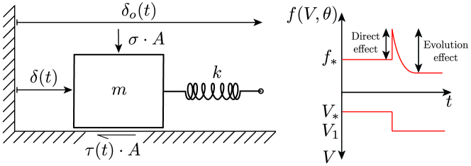
We consider the single-degree-of-freedom spring-slider elastic system depicted in Figure 1 that undergoes frictional slip. The slider is in contact with an elastic body and moves at a velocity , pulled by a point loading rate imposed at one extremity of the spring. The spring is characterized by a stiffness (per unit area of sliding contact) whose magnitude modulates the elastic force transmitted to the slider during slip motion. Normal stress and frictional law constitutive parameters and are assumed to remain constant on the contact interface. Motion is assumed to be quasi-static and the block’s inertia is neglected: i.e. the product is neglected, with being the block mass.
The equation of motion of the single-degree-of-freedom elastic system is given by the following equilibrium equation
| (14) |
where is taken to be the elastic force due to slip defined as such the single-degree of freedom counterpart to in the continuum model, is the external force proportional to the imposed displacement and likewise the single-degree of freedom counterpart to , and is the frictional force along the interface, which can be expressed, assuming a unit base area, as the product of rate- and state-dependent friction coefficient (1) and applied normal stress :
| (15) |
In rate form, Equation (14) reads
| (16) |
As stated beforehand, the frictional state variable evolves following the evolution law (5). The dimensionless parameter ranges between : i.e. between the slip and aging-law end-members. Figure 3 shows the analytical prediction of change of frictional stress in response to sudden increases or decreases of the sliding rate, for different values of . The changes are calculated for a block sliding at velocity at steady-state , until a sudden jump in velocity is imposed and eventually the new steady-state value is achieved. In this case, Equation (5) can be integrated analytically and the resulting expression can be substituted into Eq. (15) to obtain the normalised change of frictional stress between two consecutive steady states:
| (17) |
where is the slip accumulated since the velocity jump. As displayed in Figure 3 for a range of velocity jumps , a clear asymmetric behavior with the sign of the velocity jump is obtained for large values of parameter, with a slip length-scale over which stress evolves to a new steady state that depends on the magnitude of the jump itself (as predicted by aging law, yet inconsistent with laboratory friction experiments (Tullis and Weeks, , 1986; Blanpied et al., , 1998; Marone, , 1998)). On the contrary, low values of parameter lead to a more symmetric frictional response and a velocity jump-independent evolution length-scale.
At steady state, the block moves at the same speed of that of the load point, and
| (18) |
where and the subscript ss refers to steady state. If , the logarithmic dependence of the steady state shear stress (or friction coefficient) on the slip rate is negative . Hence, an increase in slip rate leads to a negative change of steady state shear stress after sufficiently slip accumulation, a condition that is commonly referred as rate-weakening condition. Vice-versa, a rate-strengthening interface experiences a positive change of steady-state shear stress upon an increase in slip rate. Since rate-strengthening interfaces are unconditionally stable, in this contribution we restrict ourselves to rate-weakening conditions, i.e. is always greater than 1.
Equations (1), (5) and (15-16) comprise a non-linear system governing the motion of the slider. Before studying the stability of such a motion in response to perturbations, we introduce characteristic scales and non-dimensionalize the governing equations to identify the key parameters that govern the motion. Similar to Ranjith and Rice, (1999), we introduce the dimensionless quantities:
| (19) |
We then combine equations (1) and (15) with (16) and (5) to eliminate the state variable and using the characteristic scales in (19), we arrive to the dimensionless autonomous system of non-linear, first-order differential equations
| (20) | |||
| (21) |
where the evolution of both normalized shear stress (or friction coefficient) and logarithmic of slip velocity (relative to the reference value ) is only function of the following dimensionless parameters: spring stiffness , rate-weakening ratio , point loading rate and finally the frictional state evolution parameter .
At steady state, equation (18) can be rewritten in dimensionless form as
| (22) |
3 Non-linear stability analysis with different frictional evolution laws
Following the work of Gu et al., (1984) and Ranjith and Rice, (1999) for the slip and aging laws, we commence the non-linear stability analysis in the phase plane by eliminating from Equations (20) and (21) and write
| (23) |
where
| (24) | |||
| (25) |
The differential form in (23) is imperfect, but we may seek a perfect differential by introducing an integrating factor , where remains to be determined. In this case, requiring
| (26) |
to be exact implies , hence
| (27) |
Substituting Equations (24) and (25) into (27) we obtain the equation that must satisfy
| (28) |
which does not lend itself to a general solution. However, for some particular cases, can be readily obtained and hence the function . Contours of provide solutions to the system since , and tangents to the contours are . If an analytical solution cannot be found, the non-linear system of equations (20-21) can be solved numerically with initial conditions.
4 Non-stationary load point (arbitrary )
4.1 Case of
We start by investigating the non-linear stability of slip for the particular case when the load point is non-stationary () and the spring stiffness is equal to the critical value obtained from linear stability analysis (6), which in dimensionless form reads
| (29) |
Owing to the mapping between spring stiffness and an equivalent stiffness of a continuum fault discussed in sub-section 1.4, we are considering either that the dimension of a finite fault is equal to its critical value predicted by linear stability analysis, or, for an unbounded fault, that the wavelength of the applied perturbation is equal to its critical value. Ruina, (1983); Rice and Ruina, (1983) showed that when infinitesimal perturbations to steady-state sliding lead to a stable and periodic slip motion with both slip and aging law: i.e., harmonic oscillations of frictional stress and sliding velocity, as shown for example in Figure 12 of Appendix A. In the non-linear regime, however, the elasto-frictional response is more complex and such a well-defined critical stiffness may not exist: systems may be linearly stable, but non-linearly unstable, and the critical stiffness may depend upon perturbation amplitude and type. In the following, we will derive analytical insights on stability and quantify critical finite perturbations that initiate unstable sliding as function of the dimensionless problem parameters.
When and , it can be shown that the solution to Equation (28) is
| (30) |
which can be used to integrate (26) and obtain the trajectories in the phase plane in the form
| (31) |

Note that the analytical trajectories (31) are valid in the slip law limit as well as for any intermediate state evolution law, except in the aging law limit for which a singularity appears. Nevertheless, one can integrate (26) using the specific solution (30) with and retrieve the aging-law trajectories of Ranjith and Rice, (1999) in the form
| (32) |
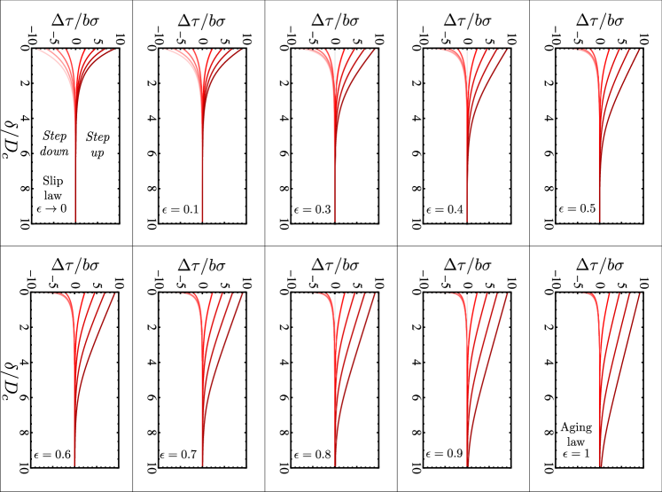
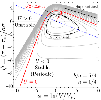
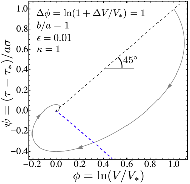
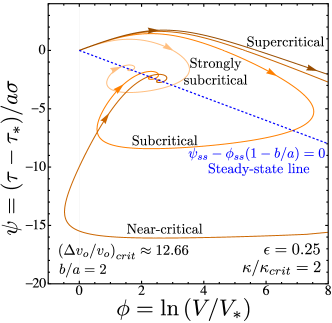
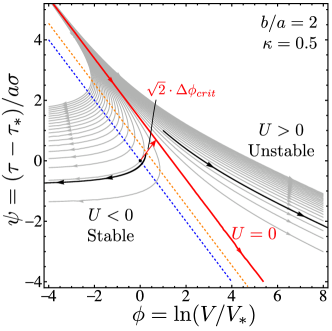
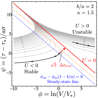
Figure 4 displays examples of constant- trajectories in the phase plane , for a given value of rate-weakening ratio , spring stiffness and different values of .
While the trajectories provide a complete solution, we may go on to focus on particular scenarios. For example, consider a block initially sliding at steady-state with the same velocity as the load point, i.e. and hence and . The initial state of the system in the phase plane reduces to a point on the steady-state line defined by Equation (22) and depicted by blue dashed lines in Figure 4. Since the reference constant velocity may be chosen arbitrary, without loss of generality here we assume that is equal to the initial loading point velocity (i.e. ), implying that the initial steady-state in the phase plane finally reduces to the origin point . When a perturbation in the form of an increase of slip rate that occurs too quickly for appreciable state evolution is introduced, the corresponding perturbation in the phase plane has changes of and of the same amount (), owing to the constant frictional state during the velocity jump Such a jump follows a direction in the phase plane oriented at from the horizontal.
From panels (a-d) in Fig. 4 we can observe that when sufficiently small perturbations to steady state are applied to the system, the state in the phase plane always jumps to a closed orbit, regardless of the value of the state evolution parameter . Closed orbits in the phase plane are stable and characterized by . To prove this, let us consider for instance orbits in the slip law limit. For a given value of and (positive or negative), Equation (31) in the limit of can be rewritten as
| (33) |
where the constant in right-hand side is always negative. From a graphical construction, it can be easily seen that there are either two or no values of that satisfy the above equation. Similarly, for specified values of , and , we can rewrite (31) in the slip law limit as
| (34) |
which shows again that it can be satisfied by either two or no values of . Since for a given value of a phase variable there exist two solutions that satisfy (31), the corresponding orbit in the phase plane must be necessarily closed. Using a similar approach, one can further show that this is valid for any values of , including the aging law limit . In this limit, however, equation (32) must be used (see also Ranjith and Rice, (1999) for more details in this case). Since closed orbits are periodic (as further highlighted by the gray arrow in Fig. 4 indicating the direction of periodic motion on closed orbits), a stable (bounded) and periodic slip motion is thus expected.
If the perturbation from an initial steady-state is sufficiently large, however, the state in the phase plane may jump from the origin point to an unstable trajectory for , i.e. an open trajectory characterized by , for which slip velocity becomes unbounded in finite time: when , it follows from (31) that
| (35) |
and, using this inequality in (21), it can be shown that
| (36) |
implies a finite-time instability, since the right-hand side of (36) is strictly positive and finite for and , and since is always bounded. Although this behavior was known to exist in the slip law limit (Gu et al., , 1984), here we find it also occurs for any , excluding the aging law limit from this interval of .
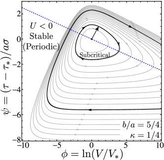
When , indeed, the trajectories form only closed orbits in the phase plane (Ranjith and Rice, , 1999), as shown in Fig. 4-d. This can be easily proved by rewriting Equation (32) as (Ranjith and Rice, , 1999)
| (37) |
where the left-hand side is constant for given values of , , , and . Therefore, like before, graphical construction of the left- and right-hand side reveals that there are either two or no values of that satisfy (37). A graphical construction of the function on the right-hand side of Equation (37) indeed resembles a parabola. When , the value of the function is . The minimum of the function instead occurs for , for which the value of the function is . Similarly, for given values of , and , Eq. (32) can be re-expressed as
| (38) |
which is satisfied by either two or no values of . A dynamic instability, therefore, can never be triggered if the frictional state evolution law follows strictly the aging law: perturbations of any size always lead to periodic oscillations, albeit with amplitudes that increase with those of the perturbations. On the contrary, when the state evolution deviates, even slightly, from the aging law, there exists a critical trajectory that separates stable (periodic) and unstable orbits, with its distance to steady state decreasing with the parameter (reaching a minimum value in the slip law limit ). This critical trajectory, represented in panels (a-c) of Figure (4) by red solid lines, corresponds to and is the curve given by, for ,
| (39) |
with its expression that further simplifies in the slip law limit () as
| (40) |
The critical trajectory is still open: given a value of , and in (39), one would get only a single value of .
We may derive the rate of divergence, since when , the inequalities (35) and (36) turn into equalities. Along the critical orbit, the variation of frictional shear stress with respect to a change in slip velocity is given by
| (41) |
whose right-hand side is always negative for any value , , and . Therefore, the above equation indicates that a continuous loss of frictional stress is expected as the slip rate diverges.
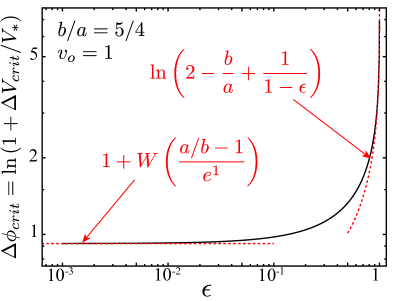
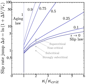
Now, a question that arises is the following: can we determine the size of the perturbation necessary to bring a system initially, say, at steady-state, to instability? Let us take, for example, a perturbation in the form of a sudden, step change in slip velocity from an initial steady state () to a new value (where may be positive or negative). The change is assumed to be too rapid for any appreciable evolution of state at that instant. Can we quantify the critical jump in slip velocity (or equivalently ) that would precipitate unstable slip? Since the jump in the phase plane occurs at constant state , at the instant of perturbation, meaning the trajectory in the phase space lies along a line , where if initially at steady-state. Thus is determined by the intersection of this line with the curve , (39): i.e., replacing the left-hand side of (39) by and solving the implicit equation for , the solution of which we dub . This solution depends on the evolution-law parameter and rate-weakening ratio . We solved numerically for using different values of in the interval , keeping the same input parameters previously reported (i.e. , and ), and limiting the solutions to those for which (i.e. neglecting the other branch of solutions for which velocity decreases lead to instability). The numerical results are displayed in the log-log plot of Figure 5-a (black solid line).
As expected, a singularity appears when : i.e. when the state tends to follow the aging (slowness) law, unconditional stability is retrieved. An asymptotic expansion of Equation (31) allows to obtain analytical solutions in terms of critical velocity jump in the limits of (aging) and (slip). With , we obtain respectively
| (42) |
in the aging law limit and
| (43) |
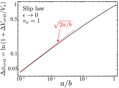
in the slip law limit, where is the Lambert -function. As shown in Figure 5-a, these analytical expressions (red dashed lines) agree with the numerical solution in the two limits: a mild singularity exists as and an -independent value of critical velocity jump occurs in the slip law limit to leading order. These results imply that a critical perturbation always exists when the frictional state evolution deviates from the aging law and . Furthermore, as , and an instability is less likely to be induced and the response to insufficient perturbation is periodic. For decreasing values of , a smaller jump in velocity is needed to trigger unstable slip, with the lowest value achieved in the slip law limit and defined in (43). Additionally, in the slip law limit, the lower is the ratio , i.e. the more pronounced is the rate-weakening condition, the lower is or : the critical perturbation that triggers an instability becomes vanishingly small (see the log-log plot in Figure 5-b), with an asymptotic scaling that follows in that limit (see red dashed line). Note also that this does not apply with rate-neutral frictional condition (see exclusion circle in Fig. 5-b). Indeed, when , the critical spring stiffness (6) is null, and is the spring stiffness due to the assumption that . In this specific case, therefore, slip stability analysis would become irrelevant. It is worth mentioning, however, that when the spring stiffness is not equal to and , the elasto-frictional coupling emerging from spring reaction and friction at the sliding interface remains. In this case, if a perturbation in the form of an instantaneous step change in slip velocity is applied to the system, the frictional stress as well as the sliding velocity experience a transient evolution from their initial (and equal) values and respectively, to the values assumed before the velocity jump, i.e. the reference steady-state values . A typical response is shown in Figure 6 which displays the trajectory in the phase plane obtained with , , and imposed initial velocity jump . The shear stress and sliding velocity spiral towards their reference steady-state values , and this is valid regardless of the perturbation strength as well as of the frictional state parameter . A dynamic instability thus can never develop with rate-neutral frictional condition and (unconditional stability).
4.2 Case of
Now, we move on to investigate the general elastic system response when the spring stiffness is not necessarily equal to the critical value obtained from linear stability analysis (29), still keeping the point loading rate non-stationary () as well as the rate weakening ratio . Under these specific conditions, we do not find the integrating factor that satisfies Equation (28) analytically. Instead, we solve the non-linear system of first-order ordinary differential equations (20-21) numerically and investigate the stability of slip subjected to sudden perturbations in slip rate and in point loading rate.
Perturbation in slip rate at fixed state
We first present the results of slip motion stability when the applied perturbation is in the form of an instantaneous jump in slip rate by an amount . Similar to what discussed in section 4.1, the normalized slip rate experiences an instantaneous increase from an initial steady-state value to a new larger value . Since the slip rate jump occurs at fixed state, the scaled shear stress increases by the same amount from its initial value . We examine the response assuming a rate-weakening ratio and a point loading rate equal to . The condition provides the constraint for the initial dimensionless slip rate and shear stress at time . We integrate numerically the governing equations (20-21) with different values of dimensionless spring stiffness and frictional state evolution parameter , and solve for the evolution of and with dimensionless time since the velocity jump. A critical jump in normalized slip rate (or in shear stress) is then identified by the jump magnitude necessary for slip motion to become unstable.
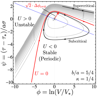
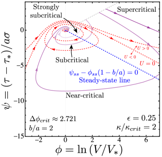
The numerical results are summarized in the stability diagram reported in Figure 7-a, which shows whether slip motion is stable or unstable upon a given slip rate jump, depending on the spring stiffness ratio and the frictional state evolution law. The blue shaded lines identify the critical jumps in slip rate for different values of parameter, with shades darkening towards the slip law limit. For a given value of and , perturbations to slip rate below the critical value do not trigger a dynamic instability, and slip rate jumps above the critical value lead to a dynamic slip motion. In Fig. 7-a, we observe that the lower is the value of , the wider is the interval of in which a dynamic instability may be triggered (for a given slip rate perturbation). The opposite occurs when the frictional state evolution tends to the aging law. In this limit, the boundary line becomes vertical and centered at (Ranjith and Rice, , 1999). When , perturbations to steady-state sliding always lead to a dynamic instability, regardless of their strength. Conditional stability, instead, occurs when .
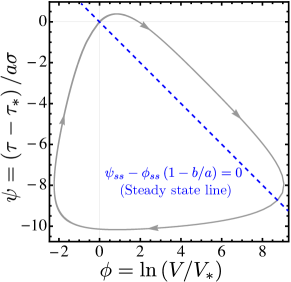
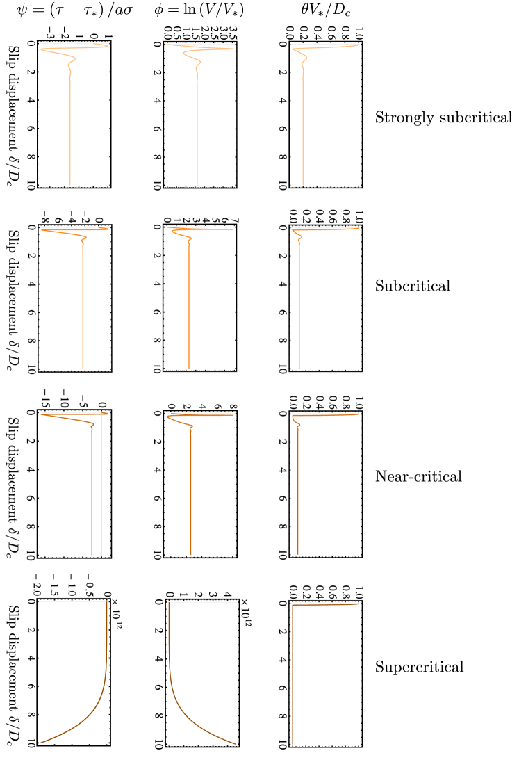
To support these results, we showcase examples of slider response in the phase plane when sub-critical, near-critical and supercritical perturbations are applied to the system (corresponding respectively to slip rate jumps below, near and above the critical value ). We fix the ratio , with , and assume the frictional state evolves following an intermediate state evolution law with (see Figure 7-a). Under these conditions, the critical jump in slip rate that initiates a dynamic instability is . Figure 7-b displays the system response in the phase plane . All trajectories (solid lines) start from direction originated from steady-state condition (see black dashed line) and, if the perturbation applied is sufficiently weak, they return to the initial steady-state condition (, ) (see strongly sub-critical, sub-critical or near-critical trajectories) or may diverge to infinity (see supercritical trajectory). Steady-state creep is thus expected following a few decaying oscillations of slip rate and shear stress on sub-critical/near-critical trajectories, as opposed to supercritical trajectories where unstable slip motion is expected. Finally, we note the function obtained for and mathematically given by (31) can be regarded as a Liapunov function for this particular case, similarly to what Gu et al., (1984) obtained for the slip law. A Liapunov function in the phase plane can be used to verify the basin of an attraction of an equilibrium state of a non-linear dynamical system: it indicates how close solutions need to be to equilibrium to be drawn to it. As shown in Fig. 7-b, the solid trajectories crossing the red dashed orbit (i.e. the strongly sub-critical, sub-critical and near-critical trajectories) and hence entering in the region of where closed dashed orbits lie, are drawn towards the steady-state point at which reaches its minimum value. The supercritical trajectory, instead, diverges from the orbit and never crosses the closed curves: unstable behavior is then expected.
Perturbation in point loading rate
We also investigate slip motion stability when the applied perturbation is not in the form of a slip rate jump, but is in the form of a jump in the point loading rate. Let us assume that initially the block slides steadily at velocity , leading to the following initial conditions for the variables and : and at time . Let us impose then a sudden perturbation to the rate of the load point displacement, increasing instantaneously its initial value from to at time . We fix the rate-weakening ratio to and, for a given arbitrary value of and , we integrate numerically the governing equations (20-21) and solve for the evolution of and with dimensionless time since the jump in loading rate (that is equivalent to solve for slip accumulated since ). A critical loading rate jump from steady-state condition is then identified, in correspondence of which slip motion becomes unstable and frictional strength rapidly decrease.
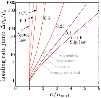
The numerical results are summarized in the plots reported in Figure 8. Although the stability diagram on the left-hand side looks qualitatively similar to the one obtained for perturbations in slip rate, the response of spring-slider in the phase plane differs. Plot (b) of Fig. 8 shows the trajectories in the phase plane obtained with the same input parameters of the previous case, i.e. , and . We observe that all the trajectories start from the initial conditions of steady-state sliding and, depending on the strength of the perturbation applied, the response evolves following different trajectories. Given that the change in load point velocity occurs at fixed state, all the trajectories share a common initial tangent. For loading rate jumps below or near the critical value, the trajectories spiral towards a new steady-state at a sliding rate of (see strongly subcritical, subcritical and near-critical trajectories in Fig. 8-b). Conversely, when the loading rate jump is above the critical value (supercritical condition), the response is characterized by a rapid and continuous loss in frictional strength and, consequently, a diverging slip rate. Slip histories of , and for those cases are shown in Figure 13 of Appendix A.
5 Stationary load point ()
Here, we investigate the stability of the slider under no active loading, i.e. a stationary load point. We set in Eq. (28) and look for the integrating factor that satisfies Equation (27) for any . It can be shown that the factor that satisfies (27) is
| (44) |
which can be used to integrate (26) and define the corresponding trajectories in the phase plane in the form
| (45) |
Note that, unlike the non-stationary case presented in section 4, here the analytical trajectories represented by (45) are valid for any intermediate state evolution law, including the end-member slip and aging laws.
Similarly to the results of the previous section 4, unstable orbits are those for which . From (45) it follows that when
| (46) |
which can be replaced into (21) along with the condition to obtain
| (47) |
Interestingly, the inequality (47) is the same found by Ranjith and Rice, (1999) for the non-linear stability analysis of the spring-slider elastic system with the aging law (3) (see their Eq. (35)). Since the right-hand side of (47) is strictly positive and finite for (with bounded), then it is clear that slip velocity becomes unbounded in finite time on positive- trajectories.
Conversely, slip motion on trajectories characterized by is always stable. To demonstrate this expectation, let us rewrite Equation (45) as
| (48) |
Since the right-hand side of the above equation tends to when , for any , (slip law limit excluded), and , there exists no value of that satisfies equation (48). Therefore, a complete loss of frictional strength never occurs on negative- trajectories when frictional state evolution deviates from the slip law (and hence instability can never take place). Rather, approaches a constant value only when and does not vanish. Indeed, the left-hand side of (48) vanishes when and , and thus the limiting shear stress value achieved at very small slip velocities (for which or is much smaller than 1) is given by
| (49) |
where in the aging law limit we retrieve the previous finding of Bhattacharya et al., (2017). However, unlimited weakening does occur in the limit of small slip velocities for the slip law (). To show this, Equation (45) can be rewritten as
| (50) |
whose right-hand side also tends to when (for , and any ). The only possible behavior that satisfies (50) is that for which , which means that also when slip is stable, and a constant minimum value of is never achieved at very small velocities.
The stability boundary that divides stable and unstable motion is the trajectory for which ,
| (51) |
The critical trajectories in this case are straight lines in the phase plane, with the ratio governing their slopes and the frictional state evolution parameter affecting solely their shift from the steady state line (22). exists if and only if
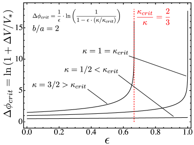
| (52) |
When this condition is violated, all the trajectories tend towards and are stable. This suggests there exists a stiffness above which an instability can never develop. This stiffness, however, increases with decreasing values of , and diverges as . In the slip law limit, therefore, perturbations to the elasto-frictional system may potentially initiate a dynamic instability, provided that their magnitudes drive the system to cross the threshold defined in (51) for the limit : . For a given value of and spring stiffness , the condition (52) also defines a critical value of above which slip motion is unconditionally stable
| (53) |
or, similarly, a critical value of above which does not exist (for a given and stiffness ), i.e.
| (54) |
When the condition (52) is violated, slip motion is always stable. However, the spring-slider elastic system may undergo a transient of self-driven slip acceleration in response to perturbations. Indeed, following from (21) and the definition of normalized state variable
| (55) |
for which the phase variables are related to it via , slip acceleration occurs when the state evolution
| (56) |
Since in this case, the limit condition for slip acceleration reduces to
| (57) |
which, with the help of (5), leads to the following condition for the dimensionless state variable
| (58) |
Now, since the dimensionless frictional stress and slip velocity jump are related to each others via , we can obtain a critical acceleration line in the phase plane that reads
| (59) |
The acceleration line in the phase plane - when it exists - is parallel to both the steady state line (22) and the critical trajectory (51). Moreover, its intersection with trajectories in the phase plane occurs at points on trajectories whose local tangent line is vertical (see for instance Figures 9 and 10).
The necessary condition for transient acceleration is
| (60) |
or, written dimensionally, when . When , we retrieve the results of Helmstetter and Shaw, (2009) for the aging law. Equation (60) implies the existence of a minimum fault dimension (or perturbation wavelength) below which a transient of self-driven slip acceleration can never develop. Again, such a minimum dimension (or wavelength) decreases with decreasing values of parameter, vanishing in the limit of . In the slip law limit, therefore, any perturbations that make the frictional stress exceed the value defined in (59), simply given by when , induce a transient slip acceleration.
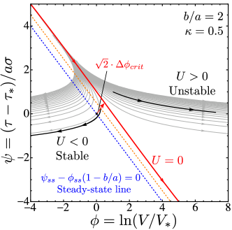
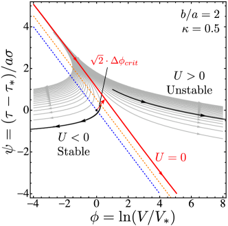
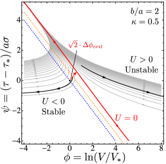
Now, similarly to section 4, imagine that an external perturbation alters suddenly the motion of the slider, bringing instantaneously its slip velocity from the steady velocity to a new, larger value . If the change in slip rate occurs faster than any appreciable state evolution can occur, then the dimensionless frictional stress increases by the same amount as that of the dimensionless slip velocity . We can identify the critical velocity perturbation as and determine its value as the distance between the origin (if we presume initial steady-state conditions) to the critical line , given by (51), along a incline. Unlike the case of a non-stationary load point, here we are able to get an analytical expression for that is valid for any and reads
| (61) |
with its existence that still depends on the condition (52) determining whether exists at all.
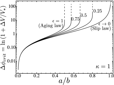
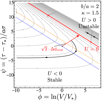
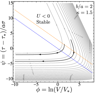
When , a dynamic instability can be triggered for any value of frictional state evolution parameter , with a critical jump in velocity that is always lower compared to any case when (for the same frictional conditions). Furthermore, the minimum value of is achieved in the slip law limit and is given by , while the maximum value of is reached in the aging law limit, for which . Figure 11-a displays how evolves as a function of , for a given rate-weakening ratio and three values of spring stiffness : lower, larger, and equal to the critical value . Examples of constant- trajectories in Figure 9 obtained with confirm the above considerations. A critical trajectory that divides stable and unstable slip motion can be clearly distinguished for any (see red solid lines in Fig. 9 or in Fig. 2 of Suppl. Material where more results with intermediate state evolution laws are included). Moreover, the critical jump from the steady-state origin (denoted by the black point along the dashed blue line) slightly increases for increasing values of , as highlighted by the length of the red arrows in panels (a-d). Finally, we can also observe that the minimum “kick” needed to induce slip acceleration is very similar for all the state evolution laws, although slightly larger finite-strength perturbations are needed in the aging law compared to the slip law. Both the critical trajectory and the acceleration line (orange dashed line) shift away from the steady state line as ; the region in the phase plane in which slip accelerates upon perturbation is wider for the aging law.
When the spring stiffness , the variation of the critical velocity jump with parameter is very similar to the non-stationary load point scenario (see Fig. 5): a singularity appears in the aging law limit. When , therefore, a dynamic instability can never be triggered regardless of the strength of the applied perturbation. Or, in other words, for slipping patches whose strength deviates from the aging law, there always exists a critical perturbation that can initiate a dynamic rupture regardless of whether the load point is stationary. The strength of such a perturbation decreases with decreasing values of , reaching its minimum value in the slip law limit. The trajectories in the phase plane depicted in Figure 3 of Supplementary Material again illustrate these considerations.
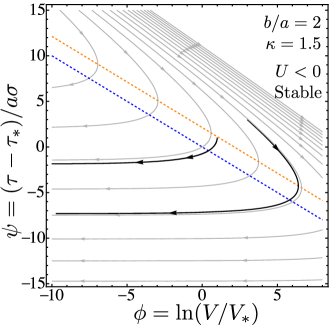
Finally, when , Figure 11-a shows that the singularity in the critical velocity jump deviates from the aging law limit and is now centered at defined by Eq. (53). This implies that there exists a range of frictional state evolution laws for which slip motion is unconditionally stable. The larger the spring stiffness is relative to the critical value , the wider is the stable interval. To illustrate this, we show in Figure 10 how the trajectories in the phase plane change with different values of , chosen to be below and above . We set and , such that . As an aside note also that with these input parameters, the necessary condition for transient slip acceleration along stable trajectories (60) is satisfied for any . From Figure 10 we can readily observe a change in elasto-frictional response when the parameter is below or above . In panels (a) and (b), which show trajectories associated with and respectively, there exists a critical line that divides stable and unstable slip motion (see the red solid line), with a jump from steady state that considerably increases as tends to (see also Fig. 4 in Suppl. Material). The region in the phase plane in which stable slip accelerates transiently is larger when (from below), and the shift of the acceleration line from steady state increases with increasing value of (see Eq. (59)). On the other hand, when (see panels (c) and (d)), there are no unstable trajectories. All the orbits in the phase plane are characterized by and hence slip motion is always stable regardless of the magnitude of the jump from steady state. Large enough perturbations, therefore, can only induce transient slip acceleration in this case. Note, however, that if a stiffer spring is considered, the acceleration condition (60) may not be satisfied for all . In Figure 5 of Supplementary Material, we present trajectories obtained with the same input parameters as above, but now the spring stiffness is larger and equal to . We can observe that when , the spring-slider motion is always stable and transient slip acceleration can only be induced when (see panels (c-d)).
So far, we have presented how the critical jump in slip velocity in response to perturbation varies with different state evolution laws and spring stiffnesses, while keeping constant the rate-weakening ratio (or its inverse). Frictional interfaces, however, exhibit different values of the parameter and depending on various factors, such as type of material of the two bodies in contact, temperature or values of effective normal stress on the interface (e.g., Blanpied et al., (1998)). It is interesting to know, therefore, how changes with the ratio for a particular state evolution law and spring stiffness. From Figure 11-b, we observe that decreases for more pronounced rate-weakening interfaces and that the state evolution law does not play a role when . All the curves, indeed, collapsed into one curve that asymptotically goes to 0 when approaches to 0. An instability can thus be triggered with small perturbations in slip motion in that limit. On the contrary, for increasing values of , increases for any . However, a particular state evolution law defines the range of in which such evolution occurs, with the maximum asymptotic value given by (54) (for a given and spring stiffness ). With the aging law, therefore, there exists an interval of for which slip motion is unconditionally stable. This interval, however, vanishes in the slip law limit: a sufficiently large perturbation can trigger an instability for any value of . Note that when , i.e. on rate-neutral interfaces an instability can never develop regardless of the strength of the perturbation applied.
6 Equivalence between the intermediate and Nagata state evolution laws
Following a series of “stress-step” experiments using a double direct shear apparatus with pre-cut granite samples, Nagata et al., (2012) proposed a revised version of rate-and-state friction law that includes a dependence on stressing rate in the form
| (62) | ||||
where the subscript N distinguishes the Nagata parameters from those of classical rate-and-state friction law presented in sub-section 1.2. If , the Nagata law reduces to the aging law (3).
The Nagata evolution law is equivalent to the intermediate law (5). Specifically, the parameters of the intermediate law are uniquely determined by the choice of the Nagata law parameters :
| (63) | ||||
This equivalency was independently recognized by Hiroyuki Noda (personal communication, 2018) and further discussed by Noda and Chang, (2023).
7 Conclusion
We have studied non-linear slip motion stability analysis of a single-degree-of-freedom elastic system with different frictional state evolution laws. Using the evolution law (5) and its parametrization via a dimensionless parameter , originally proposed by Ruina, (1983), we have investigated analytically and numerically the elastic response of the spring-slider system in the parameter space identified by scaling analysis. Our results extend and generalize those of Gu et al., (1984) and Ranjith and Rice, (1999), valid respectively only for the slip and aging laws, and provide a complete picture of slip motion stability in the non-linear regime for a range of realistic frictional state evolutions.
We have demonstrated that the critical stiffness (and by analogy to continuum faults, the nucleation length) for slip instability is not well-defined for a wide range of friction descriptions and quantified the conditions that initiate an instability as function of the governing dimensionless parameters. Remarkably, our results show that slipping patches whose state evolve following the slip law are more susceptible to transient states of self-driven slip accelerations or dynamic instabilities than those whose state evolves in an aging-law-like fashion. Moreover, a dynamic instability can nucleate on smaller faults, provided that sufficiently large perturbations are applied to the system and frictional state deviates, even slightly, from the aging law. This loading rate dependency on the nucleation process agrees with experimental observations on spatially extended frictional interfaces in which reduced dynamic-rupture nucleation lengths have been attributed to sudden, localized increases in loading rate associated with local strength heterogeneities along the frictional interface or with anthropogenic fluid injection (McLaskey and Yamashita, , 2017; Xu et al., , 2018; McLaskey, , 2019; Guérin-Marthe et al., , 2019; Gori et al., , 2021; Ji et al., , 2022). Despite the model simplicity and the simplifying assumptions, the analytical results presented here may provide support to observations of laboratory earthquake experiments and numerical findings obtained with more complex continuum models.
CrediT authorship contribution statement
Federico Ciardo: Formal analysis, Investigation, Software, Methodology, Visualization, Writing - original draft, Writing - review & editing.
Robert C. Viesca: Formal analysis, Conceptualization, Funding acquisition, Writing - review & editing, Supervision.
Declaration of competing interest
The authors declare that they have no known competing financial interests or personal relationships that could have appeared to influence the work reported in this paper.
Data availability
No data were used for the research described in this article.
Acknowledgments
This work was supported by the National Science Foundation (grant EAR-1834696).
Appendix A Appendix: Elasto-frictional response of spring-slider system subjected to finite perturbations
: periodic response
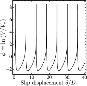
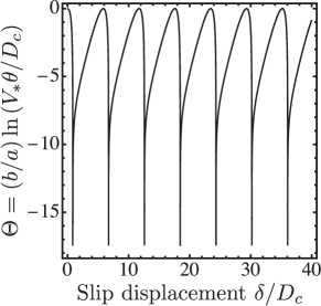
Results from linear stability analysis, valid for both slip and aging law, showed that at neutral stability the elastic response remains quasi-static and periodic upon small perturbations in slip motion (Ruina, , 1983; Rice and Ruina, , 1983). Here, we show that this is also valid in the non-linear regime with an intermediate state evolution law, provided that the applied perturbation is not large enough to trigger a dynamic instability (as discussed in sub-section 4.1).
We consider the single-degree-of-freedom spring-slider elastic system depicted in Figure (1) that slides on a rate weakening interface characterized by , with frictional state evolution that follows an intermediate law (). We assume that the spring stiffness is equal to the critical value and consider small perturbation in the form of a sudden increase of load point rate from steady-state value. Specifically, we assume a velocity jump perturbation of that is slightly below the critical value needed to initiate a dynamic instability (see Figure 8-a). Using as initial conditions the steady state conditions prior the velocity jump, i.e. and , we integrate numerically Equations (20-21) for the evolution of normalized shear stress and log of slip velocity (relative to steady state), in function of slip displacement since velocity jump.
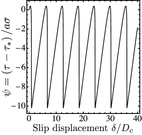
Numerical results are displayed in Figure 12. Panels (a), (b) and (c) display clear periodic oscillations of shear stress , slip velocity and normalized frictional state with slip accumulation respectively. The corresponding trajectory in the phase plane forms a closed contour (see panel (d)).
: non-periodic response
Finally, we present similar responses of spring-slider system subjected to finite perturbations in point loading rate, but now the spring stiffness is not equal to the critical value . As discussed in subsection 4.2, in this condition the elastic response is never periodic, but can be stable (with decaying oscillations amplitude) or unstable (with diverging slip rate) depending on the strength of the applied perturbation (see stability diagram in Figure 8-a). Referring to the specific scenario reported in Figure 8-b, which shows the elastic response in the phase plane when subcritical, near-critical and supercritical perturbations are applied to the system, we present in Figure 13 the corresponding evolution of , and as function of slip displacement . Consistently with the trajectories of Fig. 8-b, we can observe that shear stress, the slip velocity as well as the frictional state evolve toward new steady state values after sufficiently slip displacement, when subcritical or near-critical velocity jumps are applied to the elastic system. Conversely, a supercritical perturbation leads to a rapid and continuous loss of frictional strength and - as a result - a diverging slip rate. A new steady state condition is thus never achieved.
Appendix B Appendix: Equivalent stiffness in a continuum deformable interface
Here we provide details on how an effective stiffness can be determined for a continuum frictional interface via the solution of an associated eigenvalue problem. The eigenvalues and corresponding eigenmodes are determined by the geometry of the interface and the manner of loading. The eigenvalues correspond to the effective stiffness of each eigenmode, and may take on a discrete or continuous range of values, according to the geometry considered. Generally, when the interface is unbounded, these stiffnesses will be continuous; when the interface is finite, these will be a discrete set.
Case (A): Infinite interface between two unbounded elastic half-spaces
Let us consider an infinitely-long planar interface that divides two linear-elastic half-spaces characterized by shear modulus and Poisson’s ratio (see sketch in Figure (2)). The linear operator that determines the elastic change in shear stress in response to a given slip distribution in this case is
| (64) |
where is an equivalent shear modulus that depends on the mode of deformation: in mode II (in-plane) and in mode III (anti-plane). Using shorthand notation, we can write this as
| (65) |
where is the Hilbert transform convolution for the operator (64). We may write an eigenequation in the form of (10) as
| (66) |
where is an eigenvalue (eigenstiffness) that has units of stress per unit distance.
Given that the Hilbert transform has the property that , we may rewrite (66) as
| (67) |
In taking the derivative of (67) and using (66), we can re-express the eigenvalue problem as
| (68) |
which has solutions . Relating the wavenumber to a wavelength as , we may alternatively express the eigenstiffness as
| (69) |
which continuously varies with the choice of .
Case (B): Finite-length interface in an unbounded elastic medium
Let us consider now a similar scenario to the previous one, with the only difference being that the sliding interface is now finite in one direction and characterized by a half-length (see Figure 2, case (B)). The corresponding elastic operator now is not defined over the infinite line, but it operates over the finite interface via the following boundary integral
| (70) |
Upon scaling the spatial coordinates by and rearranging a few terms, the eigenequation (10) reads
| (71) |
where spatial coordinates are implicitly scaled by . The eigenvalue problem (71) is exactly that resulting from an instability analysis on a slip-weakening fault under plane-strain condition, and whose solution has already been obtained numerically by Uenishi and Rice, (2003). Here, we solve this eigenproblem semi-analytically using a Gauss-Chebishev quadrature with 500 integration points (see e.g. (Viesca and Garagash, , 2018)). The calculated smallest eigenvalue is
| (72) |
with the associated eigenmode that is plotted in Figure 2, case (B) (see red curve).
Case (C): Infinite interface near and parallel to a free-surface of an unbounded elastic half-space
Unlike the last two scenarios, here we consider an infinitely-long planar interface that is parallel to a free-surface of an unbounded linear-elastic half-space (see Figure 2, case (C)). We further assume that its offset from the free-surface is much smaller than the lengthscales associated with variations in distance, such that this model reduces to that of a one-dimensional compressible slab sliding on a rigid base. The elastic operator in this case reads (see supplementary materials of Viesca, 2016b )
| (73) |
where is an equivalent modulus that depends on deformation mode ( in mode II and in mode III) and spans the interval . In this particular case, the eigenequation (10) reduces to
| (74) |
which has solutions , and again, relating the wavenumber of this solution to the wavelength via , we may rewrite the eigenstiffness as
| (75) |
Case (D): Finite-length interface near and parallel to a free-surface of an unbounded elastic half-space
Perturbing the previous scenario, let the frictional interface be finite and characterized by a half-length . The elastic operator remains (73), as well as the eigenequation (74), except that now the slipping coordinate spans a finite interval . Here, however, unlike to the infinite interface case, the finiteness of the slipping region requires boundary conditions for . An appropriate choice of boundary conditions is that eigenmodes vanish at the endpoints: . Considering that solutions to (74) can be decomposed into eigenmodes that are symmetric or antisymmetric about the origin, or , imposing the boundary conditions amounts to requiring that , with being an integer. The smallest eigenstiffness is hence
| (76) |
Case (E): Circular interface in an unbounded elastic medium
Finally, we present the case of a circular interface with radius embedded in a three-dimensional linear-elastic unbounded domain. The operator in this particular scenario reads
| (77) |
where and are the complete elliptic integrals of second and first kind respectively, and . This representation is valid for a Poisson ratio , but can be considered as a leading-order approximation for a case where . Upon mapping the above integral from to using the following coordinate transformations
| (78) |
and scaling slip with a characteristic scale , the eigenequation (10) reduces to
| (79) |
which can be readily solved for the eigenvalues and the associated eigenmodes . We use Gauss-Chebyshev quadrature for the above integral representation, considering a discretization on a primary and a complimentary sets of nodes that correspond to the roots of the Chebyshev polynomials of third and fourth kind respectively, and solve the eigenvalue problem semi-analytically (Viesca and Garagash, , 2018). It is worth noting that the elastic kernel in (79) or (77) is to the leading order of Cauchy type. However, we acknowledge the presence of a weaker log singularity that compromise the accuracy of the numerical solution if not appropriately taken care of. To improve the accuracy of the quadrature, we follow a similar approach proposed by Liu et al., (2019) to regularize the logarithmic singularity. Using 500 Gauss-Chebyshev points, the smallest eigenvalue in this case is
| (80) |
Bibliography
- Ampuero and Rubin, (2008) Ampuero, J.-P. and Rubin, A. M. (2008). Earthquake nucleation on rate and state faults – aging and slip laws. Journal of Geophysical Research: Solid Earth, 113(B1). https://doi.org/10.1029/2007JB005082.
- Bhattacharya et al., (2017) Bhattacharya, P., Rubin, A. M., and Beeler, N. M. (2017). Does fault strengthening in laboratory friction experiments really depend primarily upon time and not slip? Journal of Geophysical Research, 122:6389–6430. https://doi.org/10.1002/2017JB013936.
- Bhattacharya et al., (2022) Bhattacharya, P., Rubin, A. M., Tullis, T. E., Beeler, N. M., and Okazaki, K. (2022). The evolution of rock friction is more sensitive to slip that elasped time, even at near-zero slip rates. Earth, Atmospheric, and Planetary Science, 119(30). https://doi.org/10.1073/pnas.2119462119.
- Blanpied et al., (1998) Blanpied, M. L., Marone, C. J., Lockner, D. A., Byerlee, J. D., and King, D. P. (1998). Quantitative measure of the variation in fault rheology due to fluid-rock interactions. Journal of Geophysical Research, 103(B5):9691–9712. https://doi.org/10.1029/98JB00162.
- Byerlee, (1970) Byerlee, J. D. (1970). The mechanics of stick-slip. Tectonophysics, 9:475–486. https://doi.org/10.1016/0040-1951(70)90059-4.
- Cattania, (2023) Cattania, C. (2023). A source model for earthquakes near nucleation dimension. Bull. Seism. Soc. Am., 113(3). https://doi.org/10.1785/0120220045.
- Dieterich, (1978) Dieterich, J. H. (1978). Time-dependent friction and the mechanics of stick-slip. Pure and Applied Geophysics, 116(4-5):790–806. https://doi.org/10.1007/BF00876539.
- Dieterich, (1979) Dieterich, J. H. (1979). Modeling of rock friction: 1. experimental results and constitutive equations. Journal of Geophysical Research: Solid Earth, 84(B5):2161–2168. https://doi.org/10.1029/JB084iB05p02161.
- Dieterich, (1992) Dieterich, J. H. (1992). Earthquake nucleation on faults with rate-and-state-dependent strength. Tectonophysics, 211:115–134. https://doi.org/10.1016/0040-1951(92)90055-B.
- Garagash, (2021) Garagash, D. I. (2021). Fracture mechanics of rate-and-state faults and fluid injection induced slip. Phil. Trans. R. Soc. A, 379. https://doi.org/10.1098/rsta.2020.0129.
- Gori et al., (2021) Gori, M., Rubino, V., Rosakis, A. J., and Lapusta, N. (2021). Dynamic rupture initiation and propagation in a fluid-injection laboratory setup with diagnostics across multiple temporal scales. Earth, Atmospheric, and Planetary Science, 118(51). https://doi.org/10.1073/pnas.2023433118.
- Gu et al., (1984) Gu, J.-C., Rice, J. R., Ruina, A. L., and Tse, S. T. (1984). Slip motion and stability of a single degree of freedom elastic system with rate and state dependent friction. Journal of the Mechanics and Physics of Solids, 32(3):167–196. https://doi.org/10.1016/0022-5096(84)90007-3.
- Gu and Wong, (1991) Gu, Y. and Wong, T.-F. (1991). Effects of loading velocity, stiffness, and inertia on the dynamics of a single degree of freedom spring-slider system. Journal of Geophysical Research: Solid Earth, 96(B13):21677–21691. https://doi.org/10.1029/91JB02271.
- Guérin-Marthe et al., (2019) Guérin-Marthe, S., Nielsen, S., Bird, R., Giani, S., and Di Toro, G. (2019). Earthquake nucleation size: evidence of loading rate dependence in laboratory faults. Journal of Geophysical Research, 124(689-708). https://doi.org/10.1029/2018JB016803.
- Gvirtzman and Fineberg, (2021) Gvirtzman, S. and Fineberg, J. (2021). Nucleation fronts ignite the interface rupture that initiates frictional motion. Nature Physics, 17:1037–1042. https://doi.org/10.1038/s41567-021-01299-9.
- Helmstetter and Shaw, (2009) Helmstetter, A. and Shaw, B. E. (2009). Afterslip and aftershocks in the rate-and-state friction law. Journal of Geophysical Research, 114(B01308). https://doi.org/10.1029/2007JB005077.
- Ji et al., (2022) Ji, Y., Wang, L., Hofmann, H., Kwiatek, G., and Dresen, G. (2022). High-rate fluid injection reduces the nucleation length of laboratory earthquakes on critically stressed faults in granite. Geophys. Res. Letters, 49. https://doi.org/10.1029/2022GL100418.
- Kaneko et al., (2016) Kaneko, Y., Nielsen, S., and Carpenter, B. M. (2016). The onset of laboratory earthquakes explained by nucleating rupture on a rate-and-state fault. Journal of Geophysical Research, 121(8):6071–6091. https://doi.org/10.1002/2016JB013143.
- Latour et al., (2013) Latour, S., Schubnel, A., Nielsen, S., Madariaga, R., and Vinciguerra, S. (2013). Characterization of nucleation during laboratory earthquakes. Geophys. Res. Letters, 40:5064–5069. https://doi.org/10.1002/grl.50974.
- Liu et al., (2019) Liu, D., Lecampion, B., and Garagash, D. I. (2019). Propagation of a fluid-driven fracture with fracture-length dependent apparent toughness. Engineering Fracture Mechanics, 220:106616. https://doi.org/10.1016/j.engfracmech.2019.106616.
- Marone, (1998) Marone, C. (1998). Laboratory-derived friction laws and their application to seismic faulting. Annu. Rev. Earth Planet. Sci., 26:643–696. https://doi.org/10.1146/annurev.earth.26.1.643.
- Marty et al., (2023) Marty, S., Schubnel, A., Bhat, H. S., Fukuyama, E., Latour, S., Nielsen, S., and Madariaga, R. (2023). Nucleation of laboratory earthquakes: quantitative analysis and scalings. Journal of Geophysical Research, 128(3). https://doi.org/10.1029/2022JB026294.
- McLaskey, (2019) McLaskey, G. C. (2019). Earthquake initiation from laboratory observations and implicaitons for foreshocks. Journal of Geophysical Research: Solid Earth, 124(12):12882–12904. https://doi.org/10.1029/2019JB018363.
- McLaskey and Yamashita, (2017) McLaskey, G. C. and Yamashita, F. (2017). Slow and fast ruptures on a laboratory fault controlled by loading characteristics. Journal of Geophysical Research: Solid Earth, 122:3719–3738. https://doi.org/10.1002/2016JB013681.
- Nagata et al., (2012) Nagata, K., Nakatani, M., and Yoshida, S. (2012). A revised rate- and state-dependent friction law obtained by constraining constitutive and evolution laws separately with laboratory data. Journal of Geophysical Research, 117(B02314). https://doi.org/10.1029/2011JB008818.
- Nielsen et al., (2010) Nielsen, S., Taddeucci, J., and Vinciguerra, S. (2010). Experimental observations of stick-slip instability fronts. Geophys. J. Int., 180:697–702. https://doi.org/10.1111/j.1365-246X.2009.04444.x.
- Noda and Chang, (2023) Noda, H. and Chang, C. (2023). Tertiary creep behvior for various rate- and state-dependent friction laws. Earth and Planetary Science Letters, 619(118314). https://doi.org/10.1016/j.epsl.2023.118314.
- Ohnaka and Shen, (1999) Ohnaka, M. and Shen, L.-F. (1999). Scaling of the shear rupture process from nucleation to dynamic propagation: Implications of geometric irregularity of the rupturing surfaces. Journal of Geophysical Research, 104(B1):817–844. https://doi.org/10.1029/1998JB900007.
- Okubo and Dieterich, (1984) Okubo, P. G. and Dieterich, J. H. (1984). Effects of physical fault properties on frictional instabilities produced on simulated faults. Journal of Geophysical Research, 89(B7):5817–5827. https://doi.org/10.1029/JB089iB07p05817.
- Passelègue et al., (2017) Passelègue, F. X., Latour, S., Schubnel, A., Nielsen, S., Bhat, H. S., and Madariaga, R. (2017). Influence of fault strength on precursory processes during laboratory earthquakes. In Thomas, M. Y., Mitchell, T. M., and Bhat, H. S., editors, Fault Zone Dynamic Processes: Evolution of Fault Properties During Seismic Rupture. https://doi.org/10.1002/9781119156895.ch12.
- Ranjith and Rice, (1999) Ranjith, K. and Rice, J. R. (1999). Stability of quasi-static slip in a single degree of freedom elastic system with rate and state dependent friction. Journal of the Mechanics and Physics of Solids, 47:1207–1218. https://doi.org/10.1016/S0022-5096(98)00113-6.
- Rice and Ruina, (1983) Rice, J. and Ruina, A. L. (1983). Stability of steady frictional slipping. Journal of applied mechanics, 50(2):343–349. https://doi.org/10.1115/1.3167042.
- Rice and Tse, (1986) Rice, J. R. and Tse, S. T. (1986). Dynamic motion of a single degree of freedom system following a rate and state dependent friction law. Journal of Geophysical Research, 91(B1):521–530. https://doi.org/10.1029/JB091iB01p00521.
- Rubin and Ampuero, (2005) Rubin, A. M. and Ampuero, J.-P. (2005). Earthquake nucleation on (aging) rate and state faults. Journal of Geophysical Research: Solid Earth, 110(B11). https://doi.org/10.1029/2005JB003686.
- Ruina, (1983) Ruina, A. (1983). Slip instability and state variable friction laws. Journal of Geophysical Research: Solid Earth, 88(B12):10359–10370. https://doi.org/10.1029/JB088iB12p10359.
- Tullis and Weeks, (1986) Tullis, T. E. and Weeks, J. D. (1986). Constitutive behavior and stabilty of frictional sliding of granite. Pure Appl. Geophys., 124(3):383–414. https://doi.org/10.1007/BF00877209.
- Uenishi and Rice, (2003) Uenishi, K. and Rice, J. R. (2003). Universal nucleation length for slip-weakening rupture instability under nonuniform fault loading. Journal of Geophysical Research: Solid Earth, 108(B1). https://doi.org/10.1029/2001JB001681.
- (38) Viesca, R. C. (2016a). Self-similar slip instability on interfaces with rate-and state-dependent friction. Proc. Roy. Soc. Lond. A, 472(2192):20160254. https://doi.org/10.1098/rspa.2016.0254.
- (39) Viesca, R. C. (2016b). Stable and unstable development of an interfacial sliding instability. Physical Review E, 93(6):060202. https://link.aps.org/doi/10.1103/PhysRevE.93.060202.
- Viesca, (2023) Viesca, R. C. (2023). Frictional state evolution laws and the non-linear nucleation of dynamic shear rupture. Journal of the Mechanics and Physics of Solids, 173(105221). https://doi.org/10.1016/j.jmps.2023.105221.
- Viesca and Garagash, (2018) Viesca, R. C. and Garagash, D. I. (2018). Numerical methods for coupled fracture problems. Journal of the Mechanics and Physics of Solids, 113:13–34. https://doi.org/10.1016/j.jmps.2018.01.008.
- Xu et al., (2018) Xu, S., Fukuyama, E., Yamashita, F., Mizoguchi, K., Takizawa, S., and Kawakata, H. (2018). Strain rate effect on fault slip and rupture evolution: Insigth from meter-scale rock friction experiments. Tectonophysics, 733:209–231. https://doi.org/10.1016/j.tecto.2017.11.039.