The mass effect – Variations of masses and their impact on cosmology

Abstract

We summarize and explain the current status of variations of fundamental masses in cosmology, with a particular focus on variations of the electron mass. We show that electron mass variations not only allow for significant easing of the Hubble tension but are also preferred at a decent level of significance using the latest DESI data (between $2\sigma$ and $3.6\sigma$ depending on the model and the data). This extreme success of the model is neither tightly constrained from light element abundances generated during big bang nucleosynthesis nor from post-recombination observations using quasars and atomic clocks, though future data is expected to give strong evidence in favor of or against this model. Models of baryon mass variations, on the other hand, are shown to generally not be cosmologically interesting.

1 Introduction

Our current understanding of cosmology relies heavily on our most fundamental theories of nature: quantum field theory (QFT) and general relativity (GR), describing particle physics and the gravitational interaction respectively. The outstanding accuracy at which the cosmological $\Lambda$CDM model fits our observational data thus provides a powerful validation that our most fundamental theories of physics – designed to describe local phenomena on earth and nearby astrophysical objects – can be extended as far as the very birth of our Universe.

However, the recent accumulation of theoretical and observational puzzles leaves no doubt that QFT and GR and in particular the $\Lambda$CDM cosmological standard model are not the end of the story we are trying to tell. Keeping only some of the most stringent examples, our model of particle physics will undoubtedly have to be extended in order to include the observed neutrino masses as well as very likely the dark matter, while GR will have to be extended to a quantum theory in order to describe extreme phenomena as black holes or the primordial singularity.

The $\Lambda$CDM standard model does not only inherit these theoretical challenges (such as the nature of the cold dark matter or the cosmological constant), but is also plagued by increasing observational tensions in the cosmological parameters, such as the $H_{0}$ tension that has recently risen beyond $5\sigma$ significance [1, 2, 3]. These shortcomings directly point towards the possible necessity to add to or modify the fundamental building blocks of our model [4].

Within this big picture, fundamental constants arguably play a crucial and unique role, as keystones of our theoretical constructions. They indeed set the relative magnitudes of all fundamental processes. Moreover, as they can not be computed but only measured, the constants clearly draw the borders of the predictive power of our models. Indeed, representing the limit of our theoretical understanding, they provide natural starting places to begin the search for extensions of our prevalent models. As such, looking for their possible variations in space and time gives a powerful and model independent probe of new physics. Furthermore, most of the promising theories beyond our standard models, as string theories and grand unified theories (GUTs), predict a space-time variation of the fundamental constants. The measurement of their values at different space-time points are thus a rare and privileged observable to constrain these theories.

We show in Table 2 the fundamental constants that are in principle required to describe GR and the standard model of particle physics (without neutrino masses), noting that out of the 19 constants, 2 are Higgs couplings and 9 of them are Yukawa couplings. This means that more than half of our constants are dedicated to giving particles their masses. This can be taken as an indication that our understanding of the generation of particle masses has yet to be furthered.

Due to the intricate way in which they appear within the standard model, it can be very challenging to implement variations of the masses of particles in a consistent way from first principles. It is, for example, much easier to investigate possible space-time variations of gauge couplings, such as the fine-structure constant $\alpha$. However, recent claims from cosmological observations seem to indicate that a variation of the particle’s masses in the early Universe, and more specifically the one of the electron, could significantly alleviate the $H_{0}$ tension, providing one of the most compelling models to date in that direction [5, 6, 7, 8]. This direction is further aided by the inclusion of curvature, a fact we explain in Section 2.1. As such, the variation of masses is of high importance to cosmology currently and deserves to be re-evaluated. In this work, we intend to present an updated review of the status of particle masses in this discussion in regard of the latest cosmological and local datasets.

In Section 2 we discuss constant shifts of the electron mass and its various phenomenological impacts and observational constraints, highlighting a preference for such a shift with current data. In Section 3 we dive into the topic of how such variations can in principle be derived from a more fundamental model. In Section 4 we discuss the impact of other masses in cosmology, and in Section 5 we conclude.

Before diving into the specifics of mass variations, let us make a few general notes. In this work we are not concerned with spatial variation of electron mass variations. Such spatial variations are expected to give similar effects to the ones of the fine-structure constant discussed in [9], but we leave a precise investigation for future work. Additionally, any space-time variation (including only temporal) of any fundamental constant would lead to a violation of Einstein equivalence principle (EEP), one of the cornerstones of the general theory of relativity (we comment on this point in Appendix B).

In such a case, one would be forced to introduce new fundamental forces and/or describe gravity with a non-metric theory. As such, fundamental constants can provide a powerful bridge between particle physics and gravity. Finally, when looking at mass variations, we always consider an evolution of the mass such that $m(z)/m_{0}\neq 1$ where $m_{0}=m(z=0)$ is the mass measurable in laboratory experiments today. We discuss the theoretical background of the variations of such dimensionful quantities in Appendix A.

2 Constant shift of the electron mass on cosmological scales

The simplest model for the time-variation of a particle’s mass is given by a constant offset in the early universe followed by an instantaneous transition during a time at which such a transition is difficult or impossible to observe. This simplest model allows us to study the first order effect of such mass variations without being too concerned about the actual theoretical foundations of how such mass shifts would be accomplished. As such, by design, these models are phenomenological in nature but still give valuable insights as they allow tracking the most direct impact of such a quantity on all of the relevant cosmological observables.

Of particular interest to cosmology is the shift of the electron mass. In the standard $\Lambda$CDM model the only massive particles that have a large impact on the early universe physics are the electrons, protons, and neutrons. While we discuss the status of the latter two in Section 4, we focus here on time-variations of the electron mass. During the cosmological evolution of our Universe, it is possible to identify three separate epochs at which the value of the electron mass can be relevant for observations, which are discussed in Sections 2.1, 2.2 and 2.3. Below, we detail why these three eras are especially impacted by a change of the electron mass.

Shortly after the primordial singularity the ambient kinetic energy of the propagating particles is much higher than the electron mass, making the electron effectively massless for all reactions at this time.

This soon changes during BBN, as the universe undergoes the decoupling of weak interactions (around $T\sim 1\mathrm{MeV}$, $z\sim 10^{9}$). This decoupling and the subsequent $\beta^{-}$ decay of the neutrons is tightly related to the relation between the neutron mass excess and the electron mass. The heavier the electron is, the more constrained is also the final phase-space of decays, and thus the more unlikely is the decay. This suppression of the decay rate for higher electron masses directly corresponds to a higher neutron abundance and thus leads to observably higher yields of Helium nuclei compared to hydrogen nuclei. These impacts of the electron mass on BBN through modifications of nuclear rates are detailed in Section 2.2.

After BBN, the electrons can essentially be seen as non-relativistic. However, they still partake in Compton scattering with photons (or Thompson scattering at these low energies). The threshold of where such scatterings are efficient or inefficient directly relates to the photo-ionization energies of the first atoms. The electron mass appears as a fundamental scale in most atomic transitions, dictating the binding energy and energy levels of all atoms, including most importantly for cosmology also hydrogen. As such, it directly scales the temperature scale at which recombination can take place. Indeed, this is why such a variation has a major impact on observables which rely on how long acoustic oscillations had to propagate before recombination, such as the cosmic microwave background (CMB) or the baryon acoustic oscillations (BAO). We discuss this impact in Section 2.1.

At even later times until redshift $z\gtrsim 10$ we find the cosmic dark ages during which we currently have no precise electromagnetic observations (though this might change in the distant future with 21cm mapping [10, 11, 12]), giving us no strong handle on electron mass variations during this time.

Shifts of the electron mass at the latest times are typically disfavored through high-redshift observations of electromagnetic transitions such as in quasars, as well as through current-day high-precision observations from atomic clocks and the weak equivalence principle. We comment on all of these later time probes in Section 2.3. We also comment on exceptions to such constraints in Section 4.1. As such, it is typically assumed that the electron mass has returned to its current-day value already at a redshift before such observations, for example during the dark ages.

2.1 Electron mass and the CMB

2.1.1 Theoretical background

The primary effect of the electron mass on the CMB is the effect on the parameters of recombination, such as the hydrogen binding energy or the Thompson scattering rate. The former effect is directly related to the sound horizon and the Hubble tension, while the latter is important for the CMB damping envelope.

The impact of an electron mass variation on recombination can simply be estimated by assuming chemical equilibrium (the so-called Saha equilibrium). Using $\mu_{x}$ to denote the chemical potential of species $x$ this implies $\mu_{e^{-}}+\mu_{p^{+}}=\mu_{H}$ . Using then for each particle the non-relativistic abundance

$$n_{x}=g_{x}(m_{x}T/2\pi)^{3/2}\exp[-(m_{x}-\mu_{x})/T]~{},$$ (2.1)

with mass $m_{x}$ and multiplicity $g_{x}$ for each species, one can then find that the ratio $n_{e}n_{p}/n_{H}$ does not depend on the chemical potential. Defining $x_{e}=n_{e}/n_{H}=n_{p}/n_{H}$ (assuming charge neutrality) then gives the Saha equation:

$$\frac{x_{e}^{2}}{1-x_{e}}=\left(\frac{\Omega_{b}h^{2}}{0.022}\right)^{-1}t^{3/2} \left(\frac{m_{H}}{1.00784\mathrm{amu}}\right)\left(\frac{1-Y_{\mathrm{He}}}{1-0.245}\right)\left(\frac{1+z}{1400}\right)^{-3/2}$$

$$\cdot\exp\left[41.5-41.4\left(\frac{1+z}{1400}\right)^{-1}\cdot t^{-1}\left(\frac{m_{e}}{511\mathrm{keV}}\right)(137\alpha)^{2}\right]~{},$$ (2.2)

with $t=T_{\mathrm{cmb}}/(2.7255\mathrm{K})\simeq 1$. Here we have made the dependence on all cosmological variables (including $m_{e}$) explicit. Looking at the term in the exponent we find that the redshift of recombination is $z_{*}\sim 1400$, which approximately captures the true numerically determined redshift at which the process starts. Note that in reality the reactions quickly depart from the chemical Saha equilibrium, but this simple derivation can still give us a quick intuition on the scaling of the recombination time with the electron mass. Explicitly, we see that $z_{*}\propto m_{e}$. As such, a shift of the electron mass directly shifts the recombination redshift.

It has been recently noticed in [13, 14] that a varying electron mass can also impact the sound horizon $r_{s}$ defined as

$$r_{s}=\int_{0}^{\eta_{*}}c_{s}\mathrm{d}\eta=\int_{z_{*}}^{\infty}\frac{c_{s}\mathrm{d}z^{\prime}}{H}~{},$$ (2.3)

with $\eta_{*}$ being the conformal time corresponding to $z_{*}$ , $c_{s}$ the sound speed of acoustic waves, and $H$ the Hubble parameter. Increasing the electron mass thus increases the redshift of recombination and decreases the sound horizon. This sound horizon is observable under the acoustic angle

$$\theta_{s}=\frac{r_{s}}{r_{A}}=(1+z_{*})\frac{H_{0}r_{s}}{\int_{0}^{z_{*}}\mathrm{d}z^{\prime}~{}1/E(z^{\prime})}~{},$$ (2.4)

where $E(z)=H(z)/H_{0}$ is the relative expansion rate. Since this angle is tightly constrained by observations [2], the decrease in the sound horizon perfectly compensates an increase in the Hubble constant while remaining in agreement with observations. The authors of [15] showed additionally that the angular damping scale will only be left invariant for electron mass variations (as compared to variations in $\alpha$), which heightens this degeneracy even further. Indeed, all the fundamental scales of the CMB remain intact when properly scaling the parameters $\Omega_{b}h^{2}$, $\Omega_{m}h^{2}$, and $m_{e}$ . If all fundamental scales are scaled equally, the CMB becomes almost entirely insensitive to electron mass variations. Using $\Delta_{x}$ as the fractional variation of a given parameter, we can force the three most important physical scales to equally change, enforcing

$$\Delta_{r_{s}}=\Delta_{r_{D}}=\Delta_{r_{\mathrm{eq}}}=\Delta_{z_{*}}~{}.$$ (2.5)

Here $r_{s}$ is the acoustic scale (sound horizon), $r_{D}$ the damping scale, and $r_{\mathrm{eq}}$ the equality scale. The scaling found in [15] requires

$$\Delta_{\Omega_{b}h^{2}}=\Delta_{\Omega_{m}h^{2}}=\Delta_{z_{*}}=\Delta_{m_{e}}$$ (2.6)

in terms of the underlying parameters to attain Eq. 2.5. In order to preserve the angular scales (which are the ones finally measured in the CMB), one then only needs to scale the angular diameter scale in the same way, enforcing

$$\Delta_{r_{A}}=\Delta_{z_{*}}~{}.$$ (2.7)

For this scaling, the authors of [15] find that

$$\Delta_{h}=3.23\Delta_{z_{*}}=3.23\Delta_{m_{e}}$$ (2.8)

is required in terms of the underlying parameters. If Eqs. 2.5 and 2.7 are obeyed together by using Eqs. 2.6 and 2.8, the angular scales of the CMB are barely changed and thus the variations are only very weakly constrained by CMB anisotropy data. Additionally, Eq. 2.8 implies that in this case the Hubble parameter can be increased, opening the possibility of resolving the Hubble tension without any negative observational consequences.

However, the scalings of Eqs. 2.6 and 2.8 imply

$$\Delta_{\Omega_{m}}=-5.46\Delta_{m_{e}}=-1.69\Delta_{h}~{}.$$ (2.9)

As such, solutions to the Hubble tension based on electron mass variations typically result in lower values of $\Omega_{m}$ , which has been shown in [8, 16] to be a potentially critical issue for these models. Indeed, very low values of $\Omega_{m}$ are in principle incompatible with supernovae and BAO data. However, there are two reasons for not immediately discarding this model as a solution to the Hubble tension.

First, it turns out that some new BAO observations from DESI [17] prefer mildly lower values of $\Omega_{m}$ ($\Omega_{m}=0.295\pm 0.015$). While supernovae typically prefer higher values (PantheonPLUS has $\Omega_{m}=0.334\pm 0.018$, Union3 has $\Omega_{m}=0.356\pm 0.027$, and DESY5 has $\Omega_{m}=0.352\pm 0.017$), we show below that at least for PantheonPLUS supernovae the constraint is apparently not tight enough to compete with BAO data in order to exclude such variations. Investigations of the impact of the other supernovae datasets is left to future work.

Second, there are simple modifications of the baseline model that diffuse such late-time constraints. For example, solutions have been proposed in [5, 18], in which the inclusion of additional curvature $\Omega_{k}$ weakens the constraining power of these additional probes on $\Omega_{m}$ . Below, we show that a dynamical dark energy (using the CPL model with $w=w_{0}+w_{a}(1-a)$) shows the same kind of behavior, albeit it is more susceptible to be strongly excluded with tight supernovae data.

2.1.2 Current status of measurements

As detailed in the previous subsection, a constant shift of the value of the electron mass provides a tempting path towards alleviating the Hubble tension. As such, this scenario has been frequently investigated in the literature, using different datasets and different combinations of additional parameters. The current status of measurements of the electron mass from the CMB and BAO (without BBN) is summarized in Table 1 and our contributions are shown in Fig. 1. The constraints are typically at the level of a few times $10^{-2}$ without BAO data, while they increase to a little less than $10^{-2}$ with BAO data. However, this tighter constraint can be alleviated by including additional curvature or additional dynamical variation of dark energy. We note that the latter is more sensitive to Pantheon supernovae data, as we show in table Table 1 and in Fig. 1.

We also note that each case supports a positive variation of the electron mass anywhere between 1$\sigma$ and 3$\sigma$ significance, even without adding any prior on the Hubble parameter. We note that this preference appears to at least partially be driven by the DESI BAO data with its preference for a lower $\Omega_{m}$ value, which predicts a larger electron mass from Eq. 2.9. We show evidence for this trend in Fig. 2, which presents an evident shift in the variation of the electron mass from $0.0061\pm 0.0068$ ($<1\sigma$ preference) for SDSS BAO to $0.0121\pm 0.0063$ ($\sim 2\sigma$ preference) for DESI BAO. The highest significance is found for the $m_{e}+\Omega_{k}$ model with Planck, DESI, and PantheonPLUS data at a level of $0.0188\pm 0.0052$, which prefers a variation in the electron mass at the 3.6$\sigma$ level of significance.

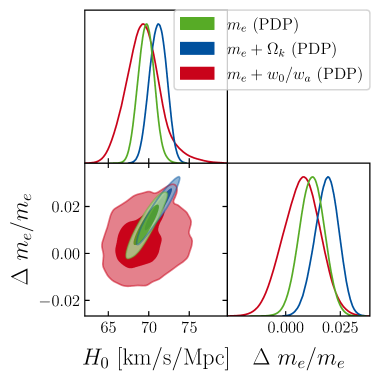
Figure 1: Constraints on variations of the electron mass ($m_{e}$), also with additional variation of curvature ($\Omega_{k}$) or CPL-dark energy ($w_{0}/w_{a}$). We show the 68% and 95% confidence contours an marginalized posteriors for P18+DESI data (PD) and also PanPLUS data (PDP), see Table 1 for references.

Model	Data	$10^{2}\Delta m_{e}/m_{e}$	$H_{0}$ [km/s/Mpc]	GT	Reference
$\Delta m_{e}/m_{e,0}$	P15	$-3.9^{+4.6}_{-7.2}$	$60^{+8}_{-16}$	1.6	[19]
$\Delta m_{e}/m_{e,0}$	P15 + SDSS	$0.39^{+0.74}_{-0.74}$	$68.1\pm 1.3$	3.0	[19]
$\Delta m_{e}/m_{e,0}$ + $\Delta\alpha/\alpha$	P15 + SDSS	$0.56\pm 0.80$	$68.1\pm 1.3$	3.0	[19]
$\Delta m_{e}/m_{e,0}$	P18	$-11.2\pm 5.9$	$46^{+9}_{-10}$	3.0	[20]
$\Delta m_{e}/m_{e,0}$	P18 + SDSS	$0.47\pm 0.66$	$68.46\pm 1.26$	2.8	[5], see also [20]
$\Delta m_{e}/m_{e,0}$ + $\Omega_{k}$	P18 + SDSS	$1.5\pm 1.8$	$69.29\pm 2.11$	1.6	[5], see also [21]
$\Delta m_{e}/m_{e,0}$	SPT+P18+SDSS+Pan	$0.3\pm 0.6$	$68.0\pm 1.1$	3.3	[18]
$\Delta m_{e}/m_{e,0}$ + $\Omega_{k}$	SPT+P18+SDSS+Pan	$0.35\pm 1.64$	$68.2\pm 1.6$	2.5	[18]
$\Delta m_{e}/m_{e,0}$ + $\Omega_{k}$ + $m_{\nu}$	SPT+P18+SDSS+Pan	$3\pm 3$	$69.8^{+1.8}_{-2.9}$	1.6	[18]
$\Delta m_{e}/m_{e,0}$	P18+DESI+SDSS+Pan	$0.92\pm 0.55$	$69.44\pm 0.84$	2.7	[22]
$\Delta m_{e}/m_{e,0}+\Omega_{k}$	P18+DESI+SDSS+Pan	$1.3\pm 1.4$	$69.7\pm 1.4$	1.9	[22]
$\Delta m_{e}/m_{e,0}$	P18+DESI	$1.21\pm 0.63$	$70.03\pm 1.06$	2.0	this work
$\Delta m_{e}/m_{e,0}+\Omega_{k}$	P18+DESI	$2.52\pm 1.85$	$70.94\pm 1.23$	1.3	this work
$\Delta m_{e}/m_{e,0}+\Omega_{k}$	P18+DESI+PanPLUS	$1.88\pm 0.52$	$71.61\pm 1.00$	1.0	this work
$\Delta m_{e}/m_{e,0}+w_{0}/w_{a}$	P18+DESI	$1.53\pm 0.63$	$70.30\pm 1.34$	1.6	this work
$\Delta m_{e}/m_{e,0}+w_{0}/w_{a}$	P18+DESI+PanPLUS	$0.72\pm 0.84$	$69.38\pm 2.17$	1.5	this work

Table 1: Review of literature constraints on the simplest implementations of a constant cosmological shift of the electron mass as well as our own contributions of Fig. 1. P15 refers to Planck 2015 CMB data (see [23]), while P18 refers to Planck 2018 CMB data (see [24]). SDSS refers to BAO during the BOSS/eBOSS era (before DESI) from the SDSS, such as DR12 LRG [25], DR14 QSO/Ly$\alpha$ [26, 27], and DR7 MGS [28], as well as small redshift BAO from 6dFGS [29]. Pan refers to Pantheon uncalibrated supernovae from [30] and PanPLUS to PantheonPLUS uncalibrated supernovae from [31]. Finally, DESI denotes data from [32, 33]. GT refers to the Gaussian tension with [3] (as a rough relative indicator).

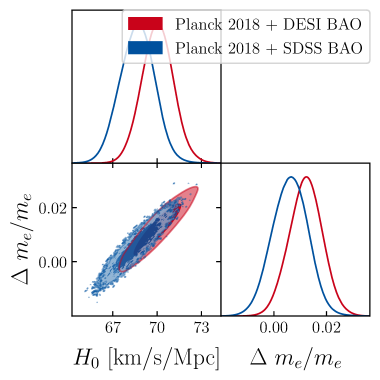
Figure 2: 68% and 95% confidence contours an marginalized posteriors for variations of the electron mass, comparing the older SDSS BAO data to the newer DESI BAO data, see Table 1 for references.

2.2 Electron mass and BBN

2.2.1 Theoretical background

It is well established that elements with higher atomic numbers have to be sequentially constructed from lighter elements, as multi-particle fusions are disfavored by the extremely small baryon-to-photon ratio $\eta_{b}\simeq 6.1\cdot 10^{-10}$. Correspondingly, the creation of the lightest heavy nucleus (Deuterium) is a Bottleneck for the creation of further heavier elements. Similar to Section 2.1.1 we can also create simplified prediction for the Deuterium generation in chemical equilibrium as

$$\frac{x_{D}}{x_{p}x_{n}}= \left(\frac{\eta_{b}}{6.1\cdot 10^{-10}}\right)\,\,t^{3/2}\,\mathfrak{m}^{3/2}\,\left(\frac{1+z}{2.74\cdot 10^{8}}\right)^{3/2}$$

$$~{}\mbox{}\quad~{}\cdot\exp\left[-34.55+t^{-1}\cdot 34.55\left(\frac{1+z}{2.74\cdot 10^{8}}\right)^{-1}\left(\frac{B_{D}}{2.22452\mathrm{MeV}}\right)\right]~{},$$ (2.10)

which predicts a redshift of $z\simeq 2.74\cdot 10^{8}$, corresponding to a photon temperature of 64keV, not far from the roughly 70keV commonly cited. Here too we have kept all constants as above and have defined for convenience

$$\mathfrak{m}=\left(\frac{m_{D}}{931.494\mathrm{MeV}}\right)\cdot\left(\frac{m_{p}}{938.272\mathrm{MeV}}\right)^{-1}\cdot\left(\frac{m_{n}}{939.565\mathrm{MeV}}\right)^{-1}~{}.$$ (2.11)

We observe that the time at which the Deuterium bottleneck is overcome is strongly dependent on the binding energy of Deuterium, which is mostly a quantity depending on strong nuclear forces, and therefore almost entirely independent of the electron mass.

However, as mentioned in the introduction of Section 2, the crucial process to consider here is $\beta^{-}$ decay. Since the weak scatterings have frozen out at BBN ($70$keV $\ll$ 1 MeV), the neutron number is essentially fixed up to $\beta^{-}$ decay. As such, there can only be as much Helium produced as there are available neutrons. Indeed, the efficiency of Helium fusion is so great that to first order it can be directly estimated from the abundance of neutrons, namely $Y_{p}=4n_{\mathrm{He}}/n_{b}\simeq 2n_{n}/(n_{n}+n_{p})$. The neutron-to-proton ratio is easily estimated using their initial abundance at the freezeout of weak interactions multiplied by the subsequent decay. Both the weak rate that determines their initial abundance and the decay rate are dependent on the electron mass. The rates can be expressed as a (complicated) function of $(m_{n}-m_{p})/m_{e}$ multiplied by an overall prefactor of $m_{e}^{5}$ [10, 34]. An increase of the electron mass results (for constant neutron-proton mass difference) overall in a decrease of the decay rate (the $m_{e}^{5}$ prefactor is overcome by the function of $(m_{n}-m_{p})/m_{e}$), thus more neutrons at the Deuterium bottleneck, leading therefore to an overall higher Helium abundance.

2.2.2 Current status of measurements

Overall, [34] argues that the BBN constraint on the variation of the electron mass should be negligible compared to Planck CMB constraints in the standard model without curvature or dynamical dark energy, but they do not show constraints from BBN alone. Here we derive the constraints from BBN using the following approach:

1. We modify the publicly available Prymordial code to accept the nuclear rates from the Parthenope code – In principle the computations could have been performed with any set of nuclear rates, but for the purpose of comparison with the rates used by default in class, we chose this set of rates (see also [35]).

2. We modify the $m_{e}$ (and later $m_{p}$/$m_{n}$) input parameters of the code, making sure to set the flag to recompute the weak rates for each computation. Since this significantly slows down the code, we chose to build an emulator (see below) to accelerate inference.

3. We evaluate a random sampling in $\{\eta_{b}\,,\Delta m_{e}/m_{e}\}$ and record the predicted element abundances and the baryon fraction for each parameter point.

4. With these predictions we build a linear interpolator in the two-dimensional parameter space that achieves an average emulation accuracy around $\sim 0.1\%$ for a range of test cases.

5. We write a likelihood using that emulator in order to compare observed element abundances with emulated/predicted ones.

The data we use are the PDG recommended abundances for $Y_{\mathrm{He}}$ and $D/H$ from [36] – $Y_{\mathrm{He}}=0.2450\pm 0.0030$ and $D/H=(2.547\pm 0.029)\cdot 10^{-5}$. We find the constraints as summarized in Fig. 3. With only BBN data the constraint on $\Delta m_{e}/m_{e}$ is very wide, up to 5% variation are allowed (whereas current 68% CL constraints from the CMB are closer to around $\sim 1\%$), in qualitative agreement with the arguments of [34]. This loose constraint persists once BAO data are added, as these do not further measure the impact of an electron mass shift beyond a change in the sound horizon. As such, through the usual calibration of the sound horizon the combination of BAO and BBN leads to constraints on $H_{0}$ , at the level of $H_{0}=67.0\pm 2.2$ km/s/Mpc.

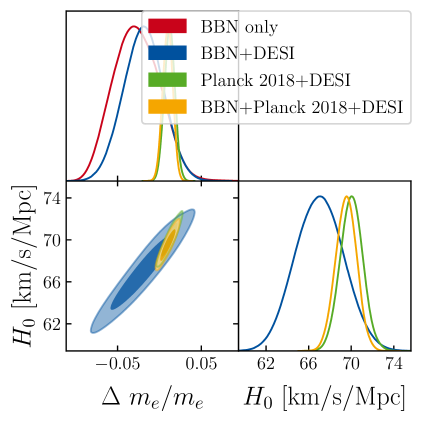
Figure 3: Same as Fig. 2, but involving data combinations with and without BBN.

Once CMB data are added back, the constraint becomes much tighter, though as before, non-zero values of the electron mass variation are preferred. The BBN does not add a lot of information beyond the Planck CMB constraints in this case, and only marginally shifts the constraint on $H_{0}$ .

We also show additional model variations in Fig. 4. BBN can slightly help constraining these more exotic variations. For example for the case of curvature $\Omega_{k}$ it reduces the constraint from $0.0252\pm 0.0185$ without BBN to $0.0150\pm 0.0055$ with BBN, which still shows an almost $3\sigma$ preference for an early electron mass variation. However, the largest range of $H_{0}$ with this data combination including BBN is given by the case of $w_{0}/w_{a}$ CPL dark energy with $H_{0}=69.3\pm 1.7$ km/s/Mpc.

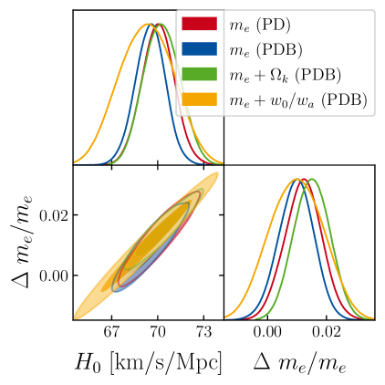
Figure 4: Same as Fig. 3, involving various models and data sets, with the same notation as in Fig. 1 and PDB including Planck2018 CMB data, DESI BAO data, and BBN abundances from [36].

Given the clear picture that neither BBN nor CMB can strongly constrain the electron mass variation, and that there even is a preference for electron mass shifts in the data, a fundamental question arises about other constraints on the variation of the electron mass.

2.3 Electron mass and the post-recombination Universe

2.3.1 Theoretical background

There are mainly two post-recombination types of measurements currently considered for constraining mass variations: astrophysical and laboratory-based. The first type of experiment measures the spectra of astrophysical objects at finite redshift. Typically, one would be interested in the absorption lines generated by cold and low density clouds surrounding bright and distant quasi stellar objects (QSO). Since the redshift of such objects is typically determined using spectral features, this measurement compares frequencies of different atomic lines. As such, the immediate dependence on the overall electron mass cancels out. For example, the Lyman-$\alpha$ transition compared to the Lyman-$\gamma$ transition always have a precise frequency ratio of $4/5$.

Instead, one uses the fact that additional corrections to energy levels, such as from rotation, vibrational, and electronic degrees of freedom (mostly for molecules) depend on ratios that are (fractional) powers of $\mu\equiv m_{p}/m_{e}$ [37, 38, 39, 40]. For example, vibrational modes typically scale as $\mu^{-1/2}$ and rotational modes as $\mu^{-1}$ [37, 41]. As such, the comparison of different types of lines allow for constraints on the mass ratio $\mu$. The precise lines used are optimized such that their dependence on the mass ratio is enhanced. For example, if two different types of energy levels are very nearby for the standard value of $\mu$, their transition frequency will be substantially more sensitive to mass variations. For example, if an electronic and the $n$-th vibrational energy levels are approximately equal, the mass-dependence of their transition is enhanced by the inverse of the small remaining transition frequency [38].

The second type of measurements are performed locally in laboratory environments using atomic clocks. It is possible to compare optical transitions with those of a hyperfine baseline. Given that the hyperfine transition depends on $\mu$ while the optical transition does not, a drift in their relative rate during a long-time laboratory experiment would signal a possible shift in $\mu$. Similar to the high-redshift measurements, different combinations of different kinds of transitions can provide different sensitivities to shifts in the mass ratio. However, many of the used transition frequencies also depend on the proton gyromagnetic ratio ($g_{p}$), which can either be assumed to be fixed to the standard model value or conservatively marginalized over.

Finally, the study of the universality of free fall can provide stringent bounds on possible mass variations, but the translation of the measurements into bounds on mass variations is not trivial. We discuss constraints from free-fall experiments in Appendix B.

2.3.2 Current status of measurements

The current status of late time measurements of possible shifts in the proton-electron mass-ratio $\mu$ using QSO can be found in [40, Tab. 2], and are typically of the order of around $10^{-6}$ to $10^{-5}$ for $z\in[0.685,4.224]$ hinting at a possible variation with a small ($\sim 1\sigma$) level of significancy [40, Eqs. (16) and (17)]. Since the highest observed redshift is around $4.2$, this means that any transition of the electron mass occurring in the dark ages would not be sensitively picked up by current experiments.

Beyond these quasar constraints there are also tight laboratory constraints on the variation of the electron mass from optical atomic clock transitions, comparing an atomic transition ($\mu^{0}$) with a hyperfine Cs137 transition ($\mu^{-1}$), which is also used for the definition of the second, see the discussion in Appendix A. We explicitly use the clocks from [40, Tab. 3] (i.e. [42, 43, 44, 45, 46, 47, 48, 49, 50]) as well as additionally [51, 52].

The resulting posteriors distributions of the time drifts of $\{\alpha,\mu,g_{p}\}$ are shown in Fig. 5, leading to constraints of a few times $10^{-7}$ in $\mathrm{d}\ln m_{e}/\mathrm{d}z$ after marginalization. While very tight, the constraint is measured at $z=0$ and therefore inapplicable to probe a cosmological transition occurring in the dark ages.

As such, the constraints that we discussed are in principle not directly applicable to the electron mass bounds above, as long as the near-instantaneous transition is kept outside of the electromagnetically observable range. However, one can wonder how to physically realize such a transition and therefore the study of these constraints will be vital in the context of our arguments on physical models in Sections 3 and 4.

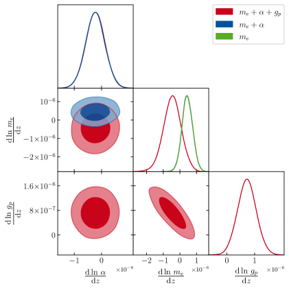
Figure 5: 68% and 95% confidence contours an marginalized posteriors for atomic clock constraints (data described in main text) on the variation of rates for a few models with different variations of underlying parameters. Note that the scale of the axis for ${\rm d}\ln\alpha/{\rm d}z$ is two orders of magnitude smaller than for ${\rm d}\ln m_{e}/{\rm d}z$.

2.4 Summarizing the viability of constant shifts of the electron mass

We recognize that the data does not disfavor constant shifts of the electron mass with a near-instantaneous transition in the dark ages. Instead, we find a slight preference for models involving such a transition typically at the $\sim 2\sigma$ level with DESI data. Especially models that feature additional late-time components such as curvature allow for a $\sim 3.6\sigma$ preference, which is robust to supernovae data and is not strongly constrained from BBN, which can only put approximate bounds at the level of $\sim 5\%$. However, beyond this purely phenomenological study, the important question arises if such a model can be realized in a consistent theory or if such a theory brings with it additional constraints that make the model unworkable.

3 Physical models: scalar fields and electron mass variation

It is apparent that an instantaneous transition of the value of the electron mass is hard to realize in any dynamical framework. However, the question of how fast a variation of the electron mass can proceed is of high importance for studying such models. If it can be shown that such a variation can not proceed fast enough, it could exclude variations of the electron mass as viable cosmological models altogether.

A more consistent implementation of varying constants must be done at the Lagrangian level. In our current understanding it is the only viable path in order to preserve consistency of the theory and conservation of all the relevant quantities and symmetries. The simplest implementations of varying masses involve one or several scalar fields. Depending on the Lagrangian implementation and its motivation, one or several constants can vary in coupled ways, typically one would expect a coupled variation of all constants within a theoretical framework motivated by GUTs or string theories [53, 54, 55].

The simplest phenomenological model one can propose is to promote $m_{e}/m_{e,0}$ itself – and thus $\mu$ – to a scalar field. A canonical Lagrangian $\mathcal{L}=\partial_{\mu}\partial^{\mu}\phi/2-V(\phi)$ can be associated to the field, which enters in the Dirac equation for fermions through $m_{e}/m_{e,0}=e^{\phi}$. Such a model, proposed by [56], generalizes the so-called Bekenstein models in which the electron charge $e/e_{0}$ is promoted to a scalar field driving variations of $\alpha$ [57, 58, 59]. To our best knowledge, the latest constraints on this model can be found in [60]. A coupled variation of both $\alpha$ and $\mu$ in this framework is discussed in [61]. From a high energy physics perspective, a more motivated approach is to add some dynamics in the Higgs sector. [62] proposed that the cosmological evolution of the Higgs field itself could lead to a dynamics of its vacuum expectation value $v$, leading to a variation of all the particle’s masses. However, as $v$ contributes almost entirely to $m_{e}$ but not as much to $m_{p}$ (see also our discussion in Section 4), such a model can be mostly understood as a varying electron mass model. Recent constraints can be found in [64]. Another option is to introduce a variation of the Yukawa couplings or to couple a new field through Yukawa-like interactions with the fermions fields. This scenario is for example possible through the Randall-Sundrum mechanism where a Goldberger-Wise scalar field couples to the fermions [65].

More generally, any GUTs attempting to unify the gauge forces at high energy or any quantum gravity theory involving extra dimensions as string theory should witness a coupled variation of all the gauge couplings and particle masses. A canonical example of this is the unavoidable presence of the dilaton field in string theory, a scalar partner of the graviton which induces a space-time variation of all the masses and gauge couplings [55, 66].

Finally, as suggested by [67], a field could be coupled to fermions through Yukawa couplings associated to a screening mechanism which makes the masses variations dependent on the local density. As such, these models could completely avoid local measurements performed on earth and allow for a significant shift of the constants during recombination in the low-density universe. The viability of such a model based on a symmetron field as a possible solution to the $H_{0}$ tension was further discussed in [68]. We will however not further discuss such mechanisms in this work.

Overall, most of the proposed models share a similar structure by involving a canonical scalar field with a specific potential and a given function relating the field to the variation of the mass $\Delta m_{e}/m_{e,0}=B_{m_{e}}(\phi)$. Witnessing that the variations of $m_{e}/m_{e,0}$ are necessarily constrained by local data to be small today, one can assume in full generality that $m_{e}/m_{e,0}\simeq 1+\zeta(\phi-\phi_{0})$, where $\phi_{0}$ is today’s value of the field and $\zeta=\partial_{\phi}B_{m_{e}}|_{\phi=\phi_{0}}$ . As such, similar arguments on the speed of the dark ages transition as the ones of [69] for $\alpha$-varying models can be applied to single field models.

3.1 Single-field constraints

Assuming that the variation of the electron mass is driven by a coupling to a single scalar field, it is necessarily subject to constraints stemming from the allowed speed of variation for such a scalar field – essentially the field cannot typically decelerate faster than through Hubble friction except in fine-tuned circumstances. These have been extensively discussed in [69], and we apply the corresponding formalism here, keeping in mind that the same caveats outlined in that work apply identically. The argument proceeds roughly as follows:

• To reach a cosmologically relevant $\Delta\mu/\mu$ at CMB times but to have a vanishing speed $\mathrm{d}\ln\mu/\mathrm{d}z$ today – as is required from Section 2.3 – the field needs to rapidly decelerate.

• The primary mechanism of deceleration is through Hubble drag, which can only proceed as $\dot{\phi}\propto a^{-3}$, and thus $\mathrm{d}\phi/\mathrm{d}\ln a\propto a^{-3}/H$.

• Since there are only three decades in redshift (most of which is during matter domination, with $H\propto a^{-3/2}$ approximately), one only finds roughly $3\cdot(3-3/2)=4.5$ orders of magnitude that the logarithmic field velocity can decrease. A more detailed calculation gives a factor around ${\sim 50\,000}$ [69].

• If a percent-level impact at recombination is desired (to give cosmological impact, see for example Sections 2.1 and 2.2), then this means that the variation of constants today could be at most $10^{-2}/50\,000\simeq 2\cdot 10^{-7}$.

For fine-structure data this kind of constraint results immediately in an almost-no-go-theorem outlined in [69], since the constraint from atomic clocks is $\mathrm{d}\ln\alpha/\mathrm{d}\ln a=(-2.3\pm 3.5)\cdot 10^{-9}$ (from Fig. 5), excluding cosmologically relevant $\alpha$ variations at the CMB times.

For variations in the electron mass, the cut is not quite as clear. This is because the constraints on the electron mass alone are at the level $\mathrm{d}\ln m_{e}/\mathrm{d}\ln a=(-4.5\pm 3.2)\cdot 10^{-7}$, degrading even further to $\mathrm{d}\ln m_{e}/\mathrm{d}\ln a=(+4.5\pm 5.4)\cdot 10^{-7}$ once marginalization over variations of the proton gyromagnetic ratio $g_{p}$ is preformed. This is at the same level as the $2\cdot 10^{-7}$ computed above. As such, in either case the constraint at CMB times through this argument remains at a few times $10^{-2}$, roughly at the limit of current CMB/BBN constraining power.

For example, the constraint without marginalization over $g_{p}$ results in a constraint on the electron mass $\left|(\Delta m_{e}/m_{e})_{z_{\mathrm{CMB}}}\right|\lesssim(2.3\pm 1.6)\%$, which according to Table 1 is about half to a third of the constraining power of Planck CMB + BAO. As such, these constraints are not yet strong enough to exclude such models (or provide another almost-no-go-theorem), though we expect future atomic clock measurements to be tightly constricting this parameter space (or lead to the detection of an ongoing drift). Already a factor of 10 in constraining power would be enough to provide an almost-no-go-theorem as in [69] for variations of the fine structure constant. It is yet unclear how much the future atomic clock measurements will be improved, as they face intrinsic noise limitation [71]. However, new concepts have been proposed which might allow to further increase the precision reached [72].

There are a few minor complications to the story. For example, one could assume that the $1.6\%$ level constraint discussed above would be quite helpful in further restricting variations of the electron mass that involve curvature or neutrino mass variations (see Table 1), but in this case the presence of curvature can actually cause a small additional deceleration of the logarithmic field speed (as the Hubble parameter will decrease more slowly compared to matter domination). While in most data combinations the curvature is constrained to have a negligible impact, if only supernovae data are used, for example, the constraint can degrade to a slowdown factor of $70\,000-90\,000$ (former: BAO, latter: Pantheon supernovae) between recombination and now, allowing even higher variations at the CMB by a factor of almost 2. However, we expect that at least the constraints presented for the model involving a shift in the electron mass, curvature, and a non-minimal neutrino mass (see Table 1, a $3\%$ level constraint) could be constrained using this method, though we leave a more detailed investigation of this exact case for future work.

Beyond this, there are the intrinsic caveats to this method, which relate to potentially fine-tuned shapes of the underlying scalar field potential or the field initial conditions, a very non-trivial coupling, or additional screening mechanisms. See [69] for a discussion of these method-inherent caveats.

3.2 Coupled case

We observe that imposing the electron mass shift to be generated at the Lagrangian level through scalar field puts generous constraints on its shift at CMB times. However, this is not the only way in which a more realistic model might impose additional constraints on the variation of the electron mass. As discussed in Section 3, many realistic models of variations of fundamental couplings (based on strings or GUTs) also impose a coupling of the fine-structure constant. For a review on this topic, see [40]. In that review, the author follows [54] and introduces a simple relationship between electron mass and fine-structure variations

$$\frac{\Delta m_{e}}{m_{e,0}}=\frac{1+S}{2}\frac{\Delta\alpha}{\alpha_{0}}~{},$$ (3.1)

where the coupling $S$ is different for most theories, and $S\to\infty$ would be the completely uncoupled theory that has been discussed so far. Cases with $S\simeq 160$ and $S=0$ have been considered so far [54, 76, 77]. It is immediately evident that any model with $S\sim\mathcal{O}(1)$ is subject to constraints of the electron mass variation coming from the fine structure constant variation. With the previous discussion of Section 3.1 we would expect such models to be generically excluded from having a large cosmological impact through their electron mass variation.

However, here too constraints can be avoided by following the limit of $S\to\infty$, in which case a given electron mass variation would cause infinitesimally small fine structure constant variations (hence recovering the independent case). Already with $S\sim 80$ the constraints from the fine structure constant and the electron mass variation would be equivalent, and for $S\gtrsim 80$ the original electron mass variation constraints would dominate. Very roughly one can approximate the final level of constraint as

$$\Delta m_{e}/m_{e}|_{z_{\mathrm{CMB}}}\sim\min\left(2\%,\frac{1+S}{2}\cdot 0.05\%\right)~{}.$$ (3.2)

As an illustration, considering the two cases studied in [77], GUTs models with $S\sim 160$ as the ones studied in [54] would still leave a lot of room for electron mass variations to solve the Hubble tension, while strongly coupled string dilaton models discussed in [78, 66, 76] with $S\sim 0$ are already too highly constrained to generate strong variations at recombination (with some additional constraints on their parameter space coming from the universality of free fall data as illustrated in [79]).

4 What about the baryon masses?

At this point, one remaining question remains to be answered. Why consider only variations of the electron mass, and not of the proton or neutron, for example? The answer can be divided into a few components, each showing an interesting angle on the answer:

• First and foremost, the variation of the electron mass is much simpler to accomplish theoretically than the variation of the baryon masses. For the former it suffices to change the Higgs vacuum or the electron Yukawa coupling. For the latter, the mass of the proton and neutron are dominated by the strong nuclear binding energy of the sea of quarks and gluons contained within, not the inherent mass of the three valence quarks. Therefore, mass variations for the baryons typically involve adjustments to the strong coupling scales, which have other far-reaching consequences.

• As such, the influence on BBN quantities is not trivial to estimate. For example, we would naively simultaneously rescale the proton and neutron masses by a similar amount at first order. However, the comparatively smaller variation of their difference is also important, as shown in [80]. As far as BBN is concerned, this difference as well as the overall mass scales are fundamental for most reactions. With an aforementioned adjustment of the strong coupling scale in general, the effect is in principle non-trivial to compute. [81] give sensitivity coefficients based on the computations of [80, 82], which for a given specific model allow computations of the primordial abundances, but are not generically interpretable independently of an underlying model that causes such a variation.

• Apart from BBN, the impact of such a variation is typically not well measurably by cosmological observables. This is because the other later processes depend primarily on electromagnetic scales, and are thus dominantly guided by $m_{e}$ or $\alpha$. Instead, the baryon mass only appears in the conversion between the baryon energy density ($\rho_{b}$) and the number count ($n_{b}$), which obeys

  $$\frac{3(H_{0}/h)^{2}}{8\pi G}\Omega_{b}h^{2}=\rho_{b}(z=0)\approx n_{b}(z=0)\cdot m_{b}=\frac{\pi^{2}}{15}T_{\mathrm{cmb}}^{4}\cdot\eta_{b}\cdot m_{b}~{}.$$ (4.1)

  While this could in principle have a large cosmological impact, in practice the baryon number count is mostly only important in comparison to the photon number count, compared to which it is already a tiny number (around $\eta_{b}\simeq 6\cdot 10^{-10}$). Changing this number by a factor of a few does change recombination, see for example Section 2.1.1, but only has a logarithmic impact. A 5% variation of the baryon mass would result in only a $0.1\%$ shift of the Saha equilibrium value, for example. Instead, the dominant effect comes from the corresponding change in the Thomson scattering rate, which results in an overall effective rescaling of the scattering rates that define the visibility function. We have

  $$\frac{\mathrm{d}\kappa}{\mathrm{d}\eta}=an_{H}x_{e}\sigma_{T}\approx\frac{3(H_{0}/h)^{2}}{8\pi G}\Omega_{b}h^{2}\cdot(1-Y_{p})\cdot\frac{1}{m_{p}}\cdot x_{e}\sigma_{T}~{}.$$ (4.2)

  This rescaling allows the CMB to put 5% level constraints on the baryon mass variation. However, it is important to note that this is only true for a somewhat fixed value of the Helium abundance $Y_{p}$ , which has a very similar re-scaling effect on the scattering rate as is evident from Eq. 4.2. As the Helium abundance is intrinsically linked to BBN, and we have seen above that BBN abundances are not generically predictable, whether there would be sensitivity to proton mass variations is difficult to answer in general.

• Even ignoring the above points, the impact on the CMB power spectrum induced by a simple rescaling of $\mathrm{d}\kappa/\mathrm{d}\eta$ is not strongly degenerate with any of the $\Lambda$CDM cosmological parameters, and therefore is not of a direct interest to the topic of cosmological tensions from the CMB (unlike the variation of the electron mass, which is degenerate with the Hubble constant, see Section 2.1).

As such, because of the different mechanism that generates the baryon masses, the strength of the impact on BBN and the CMB are hard to compute in general, and for the latter it is mostly irrelevant with regards to other degeneracies.

4.1 Simultaneous mass variations

There is a somewhat interesting artificial subcase of the mass variation parameter space in which by pure chance (or some deeper underlying theory) one has $\Delta\mu/\mu=0$ despite both $\Delta m_{e}/m_{e}\neq 0$ and $\Delta m_{p}/m_{p}\neq 0$. In this case the constraints from any local measurements (relying on comparisons of two different spectral line frequencies) can be completely circumvented, leaving only the constraints from the CMB or BBN. In practice we find that no interesting new degeneracy directions are opened up, as can be seen in Fig. 6 (note that these runs are without Helium predictions from BBN). The model with baryon mass variations ($m_{p}$) is relatively tightly constrained at the $(0.4\pm 1.4)\%$ level, while the model with both baryon and electron mass variation ($m_{p}$+$m_{e}$) is constrained at the $(-0.6\pm 3.7)\%$ level for the proton mass and the $(0.48\pm 0.81)\%$ level for the electron mass (with a long non-Gaussian tail towards higher values) without any degeneracy between the two. Finally, the solution for $\Delta\mu/\mu=0$ exhibits no additional cosmologically interesting behavior and is roughly equivalent to the case of varying only the electron mass. Note that these runs do not use Helium predictions from BBN, and as such even tighter constraints are definitely possible. However, they suffice to show that this degeneracy currently does not appear to be an interesting direction to explore beyond being a small curiosity.

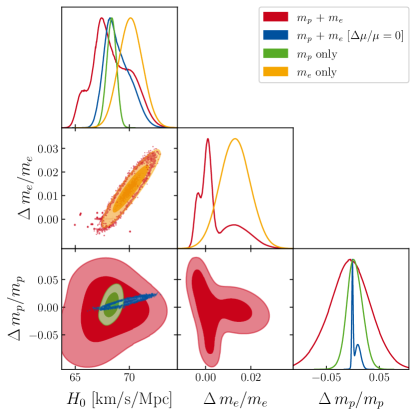
Figure 6: Same as Fig. 1 but involving models with proton mass variation as well. The used data sets are PD (Planck 2018+DESI).

5 Discussion and Conclusions

We have summarized and explained the current status of variations of the fundamental masses in cosmology, with a particular focus on the variation of the electron mass. We have shown that the simplest model of a constant shift of the electron mass results in phenomenologically interesting consequences regarding the sound horizon and the Hubble tension. We find values as high as $H_{0}=(71.61\pm 1.00)$ km/s/Mpc (see Table 1), nicely easing the Hubble tension.

We argue that these models generically suffer from a somewhat lower value of $\Omega_{m}$ . Interestingly, such a lower value of $\Omega_{m}$ appears to be favored by current BAO data (such as from DESI). We find a tantalizing $2\sigma$ preference in the baseline model for Planck+DESI BAO, and $3.6\sigma$ preference when curvature is added (when also adding the PantheonPLUS supernovae sample). A similar preference is also found when including CPL dynamical dark energy in addition to the electron mass variation. We also find that such variations are typically not strongly constrained from light element abundance measurements as the impact of electron mass variations on BBN is rather minute, confirming earlier indications by [34]. Finally, constraints from local observations have to be connected to these shifts using more realistic models. In this work we put first constraints on electron mass variations in single-field models and show that they provide only very mild direct constraints and are not yet at a level to give sufficient constraining power to restrict this solution to the Hubble tension. We note that models including screening mechanisms could avoid these bounds altogether.

Overall we summarize that electron mass variations are still an interesting solution to the Hubble tension and especially now with a tantalizing hint from DESI data. We find no evidence that the cosmologically interesting parameter space can be tightly constrained using current observations. The baryon mass variations, on the other hand, are cosmologically mostly uninteresting and hard to model generically.

Looking forward, we expect several advancements in observations to allow for more definite conclusions on this matter. First, more precise CMB data are expected shortly from ACT, SPT, Simon’s observatory, CMB-S4 and LiteBIRD [83, 84, 85, 86] along with more precise BAO data from DESI and Euclid [87, 88] and more precise post-recombination measurements [89]. Any of these upcoming measurements is expected to find either evidence for or against cosmologically relevant mass variations, giving a bright future for the mass effect.

Appendix A Mass variations and their physicality

In this section we discuss the physicality of considering variations in individual masses (as opposed to the ratios of two different masses) in Section A.2 as well as arguing about variations of physical constants more generally in Section A.3. We begin with a foreword on mass variations more generally in Section A.1

A.1 Foreword about mass variations

As displayed in Table 2, our standard model of particle physics and general relativity contains 19 fundamental constants (excluding neutrino mass parameters and unit defining constants). The masses of the fundamental particles $m_{x}$ are not considered as part of this list, but can be derived from the combination of the Yukawa couplings $h_{x}$ and the Higgs vacuum expectation value $v$ as $m_{x}=h_{x}v/2$. On the other hand, the masses of composite particles, such as all hadrons, is mostly set by the energy of the interaction between its constituents and involve the value of the gauge couplings – Effectively the masses of protons and neutrons, for example, is given by the interaction strength of the strong nuclear force with only minor corrections from the lightest quark masses.

Therefore, the particle masses are always the byproduct of interactions between more fundamental fields. Nevertheless, our standard model predicts that all masses are constant over cosmological timescales. As such, they can be seen as direct proxies of the other fundamental constants contained in Table 2 while having a more easily measurable and interpretable impact on the majority of the cosmological observables. A variation of these masses, or something mimicking this effect, would be a direct signature of new physics, implying the existence of yet unknown phenomena at play in the Higgs sector or within the gauge interactions. We discuss such models in Section 3.

A.2 Individual mass variations

The topic of what kind of constants can be considered as fundamental, and for which of these a theory of variation even makes sense, has been the topic of debate for quite a while [90, 91, 92, 39, 93]. It appears that mostly agreement has been established that the variation of dimensionless constants (such as the fine-structure constant $\alpha$) are reasonable to consider. The argument for dimensionful constants like the Higgs vacuum expectation value (VEV) or the Gravitational constant is a little more complicated, and we expand on this topic in Section A.3. For identical reasons that one would want to look at gauge invariant quantities in field theories, dimensionless ratios are indeed independent of any choice of unit and are expected to provide absolute scales to quantify the intensity of physical phenomena.

Instead, particle masses are dimensional quantities. As such, past literature typically preferred dimensionless ratios between different particle masses, such as the proton to electron mass ratio

$$\mu=\frac{m_{p}}{m_{e}}$$ (A.1)

indeed because it is also commonly appearing in considerations of atomic energy levels, such as the amplitude of the fine-structure splitting. Despite this historical prevalence we argue that variations of the individual masses are indeed reasonable to consider for two reasons:

• The varied mass can be expressed through a more fundamental unitless ratio. For example, this could be accomplished as $m_{x}/m_{\mathrm{Planck}}=m_{x}/\sqrt{\hbar c/G}$ or $m_{x}/m_{\mathrm{QCD}}=m_{x}/(\Lambda_{\mathrm{QCD}}/c^{2})$ (e.g. [94]), though we will prefer the use of $m_{x}/m_{\mathrm{hyper}}=m_{x}/(\Delta\nu_{\mathrm{Cs}}\hbar/c^{2})$. Doing so is equivalent to expressing all masses with respect to a specific mass standard ($m_{\mathrm{Planck}}$, $m_{\mathrm{QCD}}$, or $m_{\mathrm{hyper}}$) considered as fixed.

• Not only can a number of dimensionless ratios be defined, but also the way in which the different masses act to give cosmological consequences is typically through such dimensionless ratios. For the electron mass, for example, the fundamental ratio of interest is the ratio between the atomic energy levels and the ambient photon energies, which can be expressed through $m_{e}c^{2}/(k_{B}T_{\gamma})$, where the photon energy is connected to the present day CMB temperature measurement $T_{\gamma}=(1+z)T_{\mathrm{CMB}}$. Instead, the proton mass rescales the scattering rate, and therefore enters as $m_{p}/(c\rho_{b}\sigma_{T}/H)$. As such, meaningful dimensionless ratios can also be abstracted from the physical consequences of the mass variations, which are importantly different for the two masses. In such a sense, by investigating the impact of $m_{x}/m_{x,0}$ in the present work, we could have equivalently considered the impact of a variation of these dimensionless ratios.

Given their different impacts on cosmological observables and the fundamentally different way in which such mass variations are theoretically founded (Electron Yukawa+Higgs for $m_{e}$ and strong coupling+Quark Yukawa+Higgs for $m_{p}$), we argue that considering their separate variation is interesting to cosmology in principle – though as we see through the investigations within this work, only the electron mass variations can lead to interesting observable consequences.

A.3 Unit-defining constants

Compared to mass variations, we do not argue about unit-defining constants, which are also listed in Table 2 for completeness. Not only can arbitrary new units be defined using new constants (e.g. candela) but their variation is intrinsically not measurable [91, 39]. This is also evident by the lack of an uncertainty to their definition in Table 2. Therefore, variations in these unit-defining constants per-se are just unit-redefinitions and as such unphysical.

However, it is important to stress that the associated concepts could be changed instead – for the gravitational constant one can change the laws of gravitational coupling (e.g. scalar-tensor theories and especially Brans-Dicke theories [95]) or for the speed of light the physics of light-propagation, see for example [92] for an excellent description of the different concepts that usually coincide as the “speed of light” (hence our Table 2 lists the fundamental concept as a “spacetime constant” instead) and [96] for a review of consistent varying speed of light models.

Constant	Symbol	Value	Uncertainty
True constants
Strong coupling constant* – $SU(3)$	$\alpha_{s}$	0.1183	0.0009
Electromagnetic coupling constant – $SU(2)$+ $U(1)$	$\alpha_{\mathrm{EM}}^{-1}$	137.035999084	0.000000021
Weinberg angle* – $SU(2)$+ $U(1)$	$\sin^{2}(\theta_{W})$	0.23120	0.00015
Higgs VEV	$v$	246.21964GeV	0.00006GeV
Higgs mass	$m_{\mathrm{Higgs}}$	125.22GeV	0.14GeV
Electron Yukawa	$h_{e}$	$2.94\times 10^{-6}$	$7\cdot 10^{-13}$
Muon Yukawa	$h_{\mu}$	$6.07\cdot 10^{-4}$	$1.3\cdot 10^{-11}$
Tau Yukawa	$h_{\tau}$	0.01020617	0.00000052
Down Yukawa	$h_{d}$	$2.70\cdot 10^{-5}$	$4.0\cdot 10^{-7}$
Up Yukawa	$h_{u}$	$1.24\cdot 10^{-5}$	$4.0\cdot 10^{-7}$
Strange Yukawa	$h_{s}$	$5.37\cdot 10^{-4}$	$4.6\cdot 10^{-6}$
Charm Yukawa	$h_{c}$	$7.31\cdot 10^{-3}$	$2.64\cdot 10^{-6}$
Bottom Yukawa	$h_{b}$	0.024	$4.0\cdot 10^{-5}$
Top Yukawa	$h_{t}$	$0.991$	$0.002$
Quark CKM	$\sin\theta_{12}$	0.22501	0.00068
Quark CKM	$\sin\theta_{23}$	0.04183	${}^{+0.00079}_{-0.00069}$
Quark CKM	$\sin\theta_{13}$	0.003732	0.000087
Quark CKM phase	$\delta_{\mathrm{CKM}}$	1.147	0.026
Neutrino PMNS§	$\sin^{2}\theta_{12}$	0.30	0.01
Neutrino PMNS§	$\sin^{2}\theta_{23}$	0.57	0.02
Neutrino PMNS§	$\sin^{2}\theta_{13}$	0.220	0.006
Neutrino PMNS phase§	$\delta_{\mathrm{CP}}$	197∘	${}^{+42}_{-25}$∘
Neutrino mass§	$\Delta m^{2}_{\mathrm{sol}}$	$7.41\cdot 10^{-5}eV^{2}$	$0.20\cdot 10^{-5}eV^{2}$
Neutrino mass§	$\Delta m^{2}_{\mathrm{atm}}$	$2.437\cdot 10^{-3}eV^{2}$	$0.028\cdot 10^{-3}eV^{2}$
Lightest Neutrino mass§	$m_{\mathrm{lightest}}$	Not yet measured	Not yet measured
Gravitational constant	$G$	6.6743 $\cdot 10^{-11}$ $\mathrm{kg}^{-1}\mathrm{m}^{3}\mathrm{s}^{-2}$	1.5 $\cdot 10^{-15}$ $\mathrm{kg}^{-1}\mathrm{m}^{3}\mathrm{s}^{-2}$
Unit definitions
Cs hyperfine frequency	$\Delta\nu_{\mathrm{Cs}}$	9192631770 Hz	—
Elementary charge	$e$	1.602176634 $\cdot 10^{-19}$ C	—
Boltzmann constant	$k_{B}$	1.380649 $\cdot 10^{-23}$ J/K	—
Spacetime constant	$c$	299792458 m/s	—
Planck constant	$h$	6.62607015 $10^{-34}$ J/Hz	—
…	…	…	—

Table 2: All values except for the strong coupling constant (which is from [97]) are from [98]. One can also rephrase the weak ($SU(2)+U(1)$) constants through the equivalent set of $g\sim 0.65$ for $SU(2)$ and $g^{\prime}\sim 0.35$ for $U(1)$, which are related by $\sin(\theta_{W})=g^{\prime}/\sqrt{g^{\prime 2}+g^{2}}$ and $\alpha_{\mathrm{EM}}^{-1}(E=M_{Z})=g^{2}\cdot\sin(\theta_{W})$, where $\alpha_{\mathrm{EM}}^{-1}$ and $\alpha_{\mathrm{EM}}^{-1}(E=M_{Z})\simeq 127.918\pm 0.018$ are related through the usual renormalization group equations. We also have the Fermi constant $G_{F}=1/(\sqrt{2}v^{2})$ and the Higgs constants are $m_{\mathrm{Higgs}}=\sqrt{-\mu_{\mathrm{Higgs}}^{2}/2}$ and $v=m_{\mathrm{Higgs}}\sqrt{2/\lambda_{\mathrm{Higgs}}}$ with $\mu_{\mathrm{Higgs}}^{2}$ being the quadratic and $\lambda_{\mathrm{Higgs}}$ the quartic Higgs coupling. It is worth mentioning that the only dimensionful constants are the Higgs VEV ($v$, the mass is related through a dimensionless factor) and the gravitational constant, which means that the numerical value for these both are tightly related to the hyperfine frequency $\Delta\nu_{\mathrm{Cs}}$ used to define the second. All Fermion masses are simply $m_{x}=h_{x}v/\sqrt{2}$. For the neutrino properties, it is possible that the number of parameters can change depending on a future improved understanding of the origin of their oscillations.

• Measured at the Z-boson mass-equivalent energy of $M_{Z}=91.2$GeV.

• These quantities relating to the neutrino sector are not usually included in the
  standard model of particle physics. We present the fit values for normal ordering,
  see [98] for other values.

Appendix B Masses and the universality of free fall

The deviation to the universality of free fall is quantified by the Eötvos parameter comparing the acceleration of two free falling bodies $A$ and $B$:

$$\eta(A,B)=2\frac{a_{A}-a_{B}}{a_{A}+a_{B}}~{}.$$ (B.1)

Within general relativity, the Einstein Equivalence Principle (EEP) is true as an elementary axiom, hence $a_{A}=a_{B}$ and $\eta(A,B)=0\,\forall A,B$. However, this relationship can be broken in extended theories of gravity or theories of varying fundamental constants. This is because variations of fundamental constants can induce time-dependent changes of the inertial mass.

Greatly simplifying, since ${\rm d}\vec{p}/{\rm d}t=m(t)\vec{g}$ with $\vec{p}=m(t)\vec{v}$, one obtains

$$\frac{{\rm d}\ln(m)}{{\rm d}t}v+a=g~{},$$ (B.2)

and we observe that there is an additional effective force from mass variations. The mass of test atoms $A$ and $B$ is given in general by

$$m_{i}=(A_{i}-Z_{i})m_{n}+Z_{i}m_{p}+Z_{i}m_{e}-E_{B}^{\mathrm{nuclear}}-E_{B}^{\mathrm{atomic}}~{},$$ (B.3)

where $i\in\{A,B\}$, $A_{i}$ is the atomic mass number, $Z_{i}$ is the proton number, and $E_{B}$ is the binding energy (nuclear or atomic).

Therefore, when considering exclusively a time variation of $m_{e}$ (no other coupled constant variations)

$$\frac{{\rm d}\ln\left(m_{i}\right)}{{\rm d}t}=\frac{Z_{i}-\mathrm{d}(E_{i,B}^{\mathrm{atomic}})/\mathrm{d}m_{e}}{m_{i}}\,\frac{{\rm d}m_{e}}{{\rm d}t}~{},$$ (B.4)

which shows that in principle such electron mass variations would induce a non-universal free-fall for non-ionized atoms.

In principle, it is not unfeasible to compute the dependence of the atomic binding energies of common elements used in free-fall experiments (such as MICROSCOPE [99], which uses Ti and Pt) and achieves $\eta({\rm Ti},{\rm Pt})=\left(-1.5\pm 2.3(\,{\rm stat})\pm 1.5(\,{\rm syst})\right)\times 10^{-15}$.

One can estimate roughly what order of magnitude such constraints should translate to. Approximating $\mathrm{d}\ln m_{i}/\mathrm{d}t\approx\mathrm{const}$ during the timescales relevant for the experiment, we find that the $\eta\propto\Delta\mathrm{d}\ln m_{i}/\mathrm{d}t\cdot\Delta t$, where $\Delta t$ is the duration of the experiment. In that case, we would approximate that for a $\mathcal{O}(\mathrm{year})$-long duration of MICROSCOPE, one would have constraints on $\Delta\mathrm{d}\ln m_{i}/\mathrm{d}\ln a\sim 10^{-5}$. Now neglecting for the rough approximation the $\mathrm{d}E_{i,B}^{\mathrm{atomic}}/\mathrm{d}m_{e}$ term, we get $\Delta\mathrm{d}\ln m_{i}/\mathrm{d}\ln a\sim\Delta(Z_{i}/m_{i})\cdot m_{e}\cdot\mathrm{d}\ln m_{e}/\mathrm{d}\ln a$ (and $Z_{\mathrm{Ti}}=22$, $m_{\mathrm{Ti}}=47.9\,\mathrm{amu}$, $Z_{\mathrm{Pt}}=78$, $m_{\mathrm{Pt}}=195.1\,\mathrm{amu}$, which gives $\Delta(Z_{i}/m_{i})\cdot m_{e}\simeq 3\cdot 10^{-5}$), we can translate this into a bound on $\mathrm{d}\ln m_{e}/\mathrm{d}\ln a$ of the order $\mathcal{O}(1)$, which would not be competitive with atomic clock bounds, which are at the level $10^{-7}$. More typically, coupled variations of the constants will be present in a given model and thus the bound will have to be derived within the context of that given specific model (leading to much more competitive bounds). A more detailed discussion on how universality of free fall bounds can be applied to specific models can be found in [100, 55, 101]. Due to this model-dependence we do not use these bounds in the main work.

References

- [1] L. Verde, N. Schöneberg and H. Gil-Marín, A tale of many , arXiv e-prints (2023) arXiv:2311.13305 [2311.13305].
- [2] Planck collaboration, Planck 2018 results. VI. Cosmological parameters, Astron. Astrophys. 641 (2020) A6 [1807.06209].
- [3] A.G. Riess, W. Yuan, L.M. Macri, D. Scolnic, D. Brout, S. Casertano et al., A Comprehensive Measurement of the Local Value of the Hubble Constant with 1 km s-1 Mpc-1 Uncertainty from the Hubble Space Telescope and the SH0ES Team, The Astrophysical Journal Letters 934 (2022) L7 [2112.04510].
- [4] E. Di Valentino, O. Mena, S. Pan, L. Visinelli, W. Yang, A. Melchiorri et al., In the realm of the Hubble tension—a review of solutions, Class. Quant. Grav. 38 (2021) 153001 [2103.01183].
- [5] N. Schöneberg, G.F. Abellán, A. Pérez Sánchez, S.J. Witte, V. Poulin and J. Lesgourgues, The Olympics: A fair ranking of proposed models, arXiv e-prints (2021) arXiv:2107.10291 [2107.10291].
- [6] L. Hart and J. Chluba, Varying fundamental constants principal component analysis: additional hints about the Hubble tension, Mon. Not. Roy. Astron. Soc. 510 (2022) 2206 [2107.12465].
- [7] J. Chluba and L. Hart, Varying fundamental constants meet Hubble, arXiv e-prints (2023) arXiv:2309.12083 [2309.12083].
- [8] N. Lee, Y. Ali-Haïmoud, N. Schöneberg and V. Poulin, What It Takes to Solve the Hubble Tension through Modifications of Cosmological Recombination, Physical Review Letters 130 (2023) 161003 [2212.04494].
- [9] T.L. Smith, D. Grin, D. Robinson and D. Qi, Probing spatial variation of the fine-structure constant using the CMB, Phys. Rev. D 99 (2019) 043531 [1808.07486].
- [10] J. Burns, G. Hallinan, T.-C. Chang, M. Anderson, J. Bowman, R. Bradley et al., A Lunar Farside Low Radio Frequency Array for Dark Ages 21-cm Cosmology, arXiv e-prints (2021) arXiv:2103.08623 [2103.08623].
- [11] A. Mesinger, S. Furlanetto and R. Cen, 21CMFAST: a fast, seminumerical simulation of the high-redshift 21-cm signal, Monthly Notices of the Royal Astronomical Society 411 (2011) 955 [1003.3878].
- [12] A. Parsons, J.E. Aguirre, A.P. Beardsley, G. Bernardi, J.D. Bowman, P. Bull et al., A Roadmap for Astrophysics and Cosmology with High-Redshift 21 cm Intensity Mapping, in Bulletin of the American Astronomical Society, vol. 51, p. 241, Sept., 2019, DOI [1907.06440].
- [13] C.-T. Chiang and A. Slosar, Inferences of in presence of a non-standard recombination, 1811.03624.
- [14] T. Sekiguchi and T. Takahashi, Early recombination as a solution to the tension, Phys. Rev. D 103 (2021) 083507 [2007.03381].
- [15] T. Sekiguchi and T. Takahashi, Early recombination as a solution to the H0 tension, Phys. Rev. D. 103 (2021) 083507 [2007.03381].
- [16] G.P. Lynch, L. Knox and J. Chluba, Reconstructing the recombination history by combining early and late cosmological probes, arXiv e-prints (2024) arXiv:2404.05715 [2404.05715].
- [17] DESI Collaboration, A.G. Adame, J. Aguilar, S. Ahlen, S. Alam, D.M. Alexander et al., DESI 2024 VI: Cosmological Constraints from the Measurements of Baryon Acoustic Oscillations, arXiv e-prints (2024) arXiv:2404.03002 [2404.03002].
- [18] A.R. Khalife, M.B. Zanjani, S. Galli, S. Günther, J. Lesgourgues and K. Benabed, Review of Hubble tension solutions with new SH0ES and SPT-3G data, J. Cosmology Astropart. Phys. 2024 (2024) 059 [2312.09814].
- [19] L. Hart and J. Chluba, New constraints on time-dependent variations of fundamental constants using Planck data, Mon. Not. Roy. Astron. Soc. 474 (2018) 1850 [1705.03925].
- [20] L. Hart and J. Chluba, Updated fundamental constant constraints from Planck 2018 data and possible relations to the Hubble tension, Mon. Not. Roy. Astron. Soc. 493 (2020) 3255 [1912.03986].
- [21] Y. Toda, W. Giarè, E. Özülker, E. Di Valentino and S. Vagnozzi, Combining pre- and post-recombination new physics to address cosmological tensions: case study with varying electron mass and a sign-switching cosmological constant, 2407.01173.
- [22] O. Seto and Y. Toda, DESI constraints on varying electron mass model and axion-like early dark energy, arXiv e-prints (2024) arXiv:2405.11869 [2405.11869].
- [23] Planck collaboration, Planck 2015 results. XIV. Dark energy and modified gravity, Astron. Astrophys. 594 (2016) A14 [1502.01590].
- [24] Planck Collaboration, N. Aghanim, Y. Akrami, M. Ashdown, J. Aumont, C. Baccigalupi et al., Planck 2018 results. V. CMB power spectra and likelihoods, Astronomy and Astrophysics 641 (2020) A5 [1907.12875].
- [25] BOSS collaboration, The clustering of galaxies in the completed SDSS-III Baryon Oscillation Spectroscopic Survey: cosmological analysis of the DR12 galaxy sample, Mon. Not. Roy. Astron. Soc. 470 (2017) 2617 [1607.03155].
- [26] eBOSS collaboration, Baryon acoustic oscillations from the cross-correlation of Ly absorption and quasars in eBOSS DR14, Astron. Astrophys. 629 (2019) A86 [1904.03430].
- [27] eBOSS collaboration, Baryon acoustic oscillations at z = 2.34 from the correlations of Ly absorption in eBOSS DR14, Astron. Astrophys. 629 (2019) A85 [1904.03400].
- [28] A.J. Ross, L. Samushia, C. Howlett, W.J. Percival, A. Burden and M. Manera, The clustering of the SDSS DR7 main Galaxy sample – I. A 4 per cent distance measure at , Mon. Not. Roy. Astron. Soc. 449 (2015) 835 [1409.3242].
- [29] F. Beutler, C. Blake, M. Colless, D.H. Jones, L. Staveley-Smith, L. Campbell et al., The 6dF Galaxy Survey: baryon acoustic oscillations and the local Hubble constant, Monthly Notices of the Royal Astronomical Society 416 (2011) 3017 [1106.3366].
- [30] D.M. Scolnic, D.O. Jones, A. Rest, Y.C. Pan, R. Chornock, R.J. Foley et al., The Complete Light-curve Sample of Spectroscopically Confirmed SNe Ia from Pan-STARRS1 and Cosmological Constraints from the Combined Pantheon Sample, The Astrophysical Journal 859 (2018) 101 [1710.00845].
- [31] D. Scolnic et al., The Pantheon+ Analysis: The Full Data Set and Light-curve Release, Astrophys. J. 938 (2022) 113 [2112.03863].
- [32] DESI collaboration, DESI 2024 III: Baryon Acoustic Oscillations from Galaxies and Quasars, 2404.03000.
- [33] DESI collaboration, DESI 2024 IV: Baryon Acoustic Oscillations from the Lyman Alpha Forest, 2404.03001.
- [34] O. Seto and Y. Toda, Big bang nucleosynthesis constraints on varying electron mass solution to the Hubble tension, Phys. Rev. D. 107 (2023) 083512 [2206.13209].
- [35] N. Schöneberg, The 2024 BBN baryon abundance update, JCAP 06 (2024) 006 [2401.15054].
- [36] Particle Data Group collaboration, Review of Particle Physics, PTEP 2022 (2022) 083C01.
- [37] P. Jansen, H.L. Bethlem and W. Ubachs, Perspective: Tipping the scales - search for drifting constants from molecular spectra, J. Chem. Phys. 140 (2014) 010901 [1312.1875].
- [38] W. Ubachs, R. Buning, K.S.E. Eikema and E. Reinhold, On a possible variation of the proton-to-electron mass ratio: H2 spectra in the line of sight of high-redshift quasars and in the laboratory, Journal of Molecular Spectroscopy 241 (2007) 155.
- [39] J.-P. Uzan, Varying Constants, Gravitation and Cosmology, Living Reviews in Relativity 14 (2011) 2 [1009.5514].
- [40] C.J.A.P. Martins, The status of varying constants: a review of the physics, searches and implications, Reports on Progress in Physics 80 (2017) 126902 [1709.02923].
- [41] S.G. Karshenboim, Some possibilities for laboratory searches for variations of fundamental constants, Can. J. Phys. 78 (2000) 639 [physics/0008051].
- [42] T. Rosenband, D.B. Hume, P.O. Schmidt, C.W. Chou, A. Brusch, L. Lorini et al., Frequency ratio of al¡sup¿+¡/sup¿ and hg¡sup¿+¡/sup¿ single-ion optical clocks; metrology at the 17th decimal place, Science 319 (2008) 1808 [https://www.science.org/doi/pdf/10.1126/science.1154622].
- [43] N. Leefer, C.T.M. Weber, A. Cingöz, J.R. Torgerson and D. Budker, New Limits on Variation of the Fine-Structure Constant Using Atomic Dysprosium, Physical Review Letters 111 (2013) 060801 [1304.6940].
- [44] A. Shelkovnikov, R.J. Butcher, C. Chardonnet and A. Amy-Klein, Stability of the proton-to-electron mass ratio, Phys. Rev. Lett. 100 (2008) 150801 [0803.1829].
- [45] M. Fischer, N. Kolachevsky, M. Zimmermann, R. Holzwarth, T. Udem, T.W. Hansch et al., Precision Spectroscopy of Atomic Hydrogen and Variations of Fundamental Constants, in Astrophysics, Clocks and Fundamental Constants, S.G. Karshenboim and E. Peik, eds., vol. 648, pp. 209–227 (2004), DOI.
- [46] M. Abgrall, B. Chupin, L. De Sarlo, J. Guéna, P. Laurent, Y. Le Coq et al., Atomic fountains and optical clocks at SYRTE: Status and perspectives, Comptes Rendus Physique 16 (2015) 461 [1507.04623].
- [47] T.M. Fortier et al., Precision atomic spectroscopy for improved limits on variation of the fine structure constant and local position invariance, Phys. Rev. Lett. 98 (2007) 070801.
- [48] C. Tamm, N. Huntemann, B. Lipphardt, V. Gerginov, N. Nemitz, M. Kazda et al., Cs-based optical frequency measurement using cross-linked optical and microwave oscillators, Phys. Rev. A. 89 (2014) 023820 [1310.8190].
- [49] N. Huntemann, B. Lipphardt, C. Tamm, V. Gerginov, S. Weyers and E. Peik, Improved Limit on a Temporal Variation of mp/me from Comparisons of Yb+ and Cs Atomic Clocks, Physical Review Letters 113 (2014) 210802 [1407.4408].
- [50] J. Guéna et al., First international comparison of fountain primary frequency standards via a long distance optical fiber link, Metrologia 54 (2017) 348 [1703.02892].
- [51] R. Lange, N. Huntemann, J.M. Rahm, C. Sanner, H. Shao, B. Lipphardt et al., Improved limits for violations of local position invariance from atomic clock comparisons, Phys. Rev. Lett. 126 (2021) 011102 [2010.06620].
- [52] M. Filzinger, S. Dörscher, R. Lange, J. Klose, M. Steinel, E. Benkler et al., Improved Limits on the Coupling of Ultralight Bosonic Dark Matter to Photons from Optical Atomic Clock Comparisons, Phys. Rev. Lett. 130 (2023) 253001 [2301.03433].
- [53] B.A. Campbell and K.A. Olive, Nucleosynthesis and the time dependence of fundamental couplings, Physics Letters B 345 (1995) 429 [hep-ph/9411272].
- [54] A. Coc, N.J. Nunes, K.A. Olive, J.-P. Uzan and E. Vangioni, Coupled Variations of Fundamental Couplings and Primordial Nucleosynthesis, Phys. Rev. D 76 (2007) 023511 [astro-ph/0610733].
- [55] T. Damour and A.M. Polyakov, The string dilation and a least coupling principle, Nuclear Physics B 423 (1994) 532 [hep-th/9401069].
- [56] J.D. Barrow and J. Magueijo, Cosmological constraints on a dynamical electron mass, Phys. Rev. D 72 (2005) 043521 [astro-ph/0503222].
- [57] J.D. Bekenstein, Fine-structure constant: Is it really a constant?, Phys. Rev. D. 25 (1982) 1527.
- [58] H.B. Sandvik, J.D. Barrow and J. Magueijo, A Simple Cosmology with a Varying Fine Structure Constant, Physical Review Letters 88 (2002) 031302 [astro-ph/0107512].
- [59] K.A. Olive and M. Pospelov, Evolution of the fine structure constant driven by dark matter and the cosmological constant, Phys. Rev. D. 65 (2002) 085044 [hep-ph/0110377].
- [60] C.G. Scóccola, M.E. Mosquera, S.J. Landau and H. Vucetich, Time variation of the electron mass in the early universe and the barrow-magueijo model, The Astrophysical Journal 681 (2008) 737.
- [61] P.P. Avelino, Cosmological evolution of and and the dynamics of dark energy, Phys. Rev. D. 78 (2008) 043516 [0804.3394].
- [62] X. Calmet, Cosmological evolution of the Higgs boson’s vacuum expectation value, European Physical Journal C 77 (2017) 729 [1707.06922].
- [63] L.W.H. Fung, L. Li, T. Liu, H.N. Luu, Y.-C. Qiu and S.H.H. Tye, Axi-Higgs cosmology, J. Cosmology Astropart. Phys. 2021 (2021) 057 [2102.11257].
- [64] S. Chakrabarti, Cosmic variation of proton-to-electron mass ratio with an interacting Higgs scalar field, Monthly Notices of the Royal Astronomical Society 506 (2021) 2518 [2107.00543].
- [65] B. von Harling and G. Servant, Cosmological evolution of Yukawa couplings: the 5D perspective, Journal of High Energy Physics 2017 (2017) 77 [1612.02447].
- [66] T. Chiba, T. Kobayashi, M. Yamaguchi and J. Yokoyama, Time variation of the proton-electron mass ratio and the fine structure constant with a runaway dilaton, Phys. Rev. D. 75 (2007) 043516 [hep-ph/0610027].
- [67] K.A. Olive and M. Pospelov, Environmental dependence of masses and coupling constants, Phys. Rev. D. 77 (2008) 043524 [0709.3825].
- [68] R. Solomon, G. Agarwal and D. Stojkovic, Environment dependent electron mass and the Hubble constant tension, Phys. Rev. D. 105 (2022) 103536 [2201.03127].
- [69] L. Vacher and N. Schöneberg, Incompatibility of fine-structure constant variations at recombination with local observations, Phys. Rev. D. 109 (2024) 103520 [2403.02256].
- [70] M. Filzinger, S. Dörscher, R. Lange, J. Klose, M. Steinel, E. Benkler et al., Improved limits on the coupling of ultralight bosonic dark matter to photons from optical atomic clock comparisons, arXiv e-prints (2023) arXiv:2301.03433 [2301.03433].
- [71] A.D. Ludlow, M.M. Boyd, J. Ye, E. Peik and P.O. Schmidt, Optical atomic clocks, Reviews of Modern Physics 87 (2015) 637 [1407.3493].
- [72] J.M. Robinson, M. Miklos, Y.M. Tso, C.J. Kennedy, T. Bothwell, D. Kedar et al., Direct comparison of two spin-squeezed optical clock ensembles at the 10-17 level, Nature Phys. 20 (2024) 208 [2211.08621].
- [73] E. Peik and C. Tamm, Nuclear laser spectroscopy of the 3.5 ev transition in th-229, Europhysics Letters 61 (2003) 181.
- [74] V.V. Flambaum, Enhanced effect of temporal variation of the fine structure constant and strong interaction in Th-229, Phys. Rev. A 73 (2006) 034101 [physics/0604188].
- [75] P. Fadeev, J.C. Berengut and V.V. Flambaum, Sensitivity of nuclear clock transition to variation of the fine-structure constant, Phys. Rev. A 102 (2020) 052833.
- [76] M. Nakashima, K. Ichikawa, R. Nagata and J. Yokoyama, Constraining the time variation of the coupling constants from cosmic microwave background: effect of QCD, J. Cosmology Astropart. Phys. 2010 (2010) 030 [0910.0742].
- [77] C.J.A.P. Martins, Primordial nucleosynthesis with varying fundamental constants. Degeneracies with cosmological parameters, Astronomy and Astrophysics 646 (2021) A47 [2012.10505].
- [78] T. Damour, F. Piazza and G. Veneziano, Violations of the equivalence principle in a dilaton-runaway scenario, Phys. Rev. D. 66 (2002) 046007 [hep-th/0205111].
- [79] L. Vacher, N. Schöneberg, J.D.F. Dias, C.J.A.P. Martins and F. Pimenta, Runaway dilaton models: Improved constraints from the full cosmological evolution, Phys. Rev. D. 107 (2023) 104002 [2301.13500].
- [80] A. Coc, N.J. Nunes, K.A. Olive, J.-P. Uzan and E. Vangioni, Coupled variations of fundamental couplings and primordial nucleosynthesis, Phys. Rev. D. 76 (2007) 023511 [astro-ph/0610733].
- [81] M.T. Clara and C.J.A.P. Martins, Primordial nucleosynthesis with varying fundamental constants. Improved constraints and a possible solution to the lithium problem, Astronomy and Astrophysics 633 (2020) L11 [2001.01787].
- [82] T. Dent, S. Stern and C. Wetterich, Primordial nucleosynthesis as a probe of fundamental physics parameters, Phys. Rev. D. 76 (2007) 063513 [0705.0696].
- [83] S. Aiola, E. Calabrese, L. Maurin, S. Naess, B.L. Schmitt, M.H. Abitbol et al., The Atacama Cosmology Telescope: DR4 maps and cosmological parameters, J. Cosmology Astropart. Phys. 2020 (2020) 047 [2007.07288].
- [84] J.T. Sayre, C.L. Reichardt, J.W. Henning, P.A.R. Ade, A.J. Anderson, J.E. Austermann et al., Measurements of B -mode polarization of the cosmic microwave background from 500 square degrees of SPTpol data, Phys. Rev. D. 101 (2020) 122003 [1910.05748].
- [85] The Simons Observatory collaboration, The Simons Observatory, in BAAS, vol. 51, p. 147, Sept., 2019 [1907.08284].
- [86] LiteBIRD Collaboration, E. Allys, K. Arnold, J. Aumont, R. Aurlien, S. Azzoni et al., Probing cosmic inflation with the LiteBIRD cosmic microwave background polarization survey, Progress of Theoretical and Experimental Physics 2023 (2023) 042F01 [2202.02773].
- [87] A. Dey, D.J. Schlegel, D. Lang, R. Blum, K. Burleigh, X. Fan et al., Overview of the desi legacy imaging surveys, The Astronomical Journal 157 (2019) 168.
- [88] Euclid Collaboration, Y. Mellier, Abdurro’uf, J.A. Acevedo Barroso, A. Achúcarro, J. Adamek et al., Euclid. I. Overview of the Euclid mission, arXiv e-prints (2024) arXiv:2405.13491 [2405.13491].
- [89] J. Liske, G. Bono, J. Cepa et al., Top Level Requirements For ELT-HIRES, Tech. Rep. Document ESO 204697 Version 1 (2014).
- [90] M.J. Duff, L.B. Okun and G. Veneziano, Trialogue on the number of fundamental constants, Journal of High Energy Physics 2002 (2002) 023 [physics/0110060].
- [91] M.J. Duff, Comment on time-variation of fundamental constants, arXiv e-prints (2002) hep [hep-th/0208093].
- [92] G.F.R. Ellis and J.-P. Uzan, c is the speed of light, isn’t it?, American Journal of Physics 73 (2005) 240 [gr-qc/0305099].
- [93] M.J. Duff, How fundamental are fundamental constants?, Contemporary Physics 56 (2015) 35 [1412.2040].
- [94] T. Kobayashi, A. Takamizawa, D. Akamatsu, A. Kawasaki, A. Nishiyama, K. Hosaka et al., Search for Ultralight Dark Matter from Long-Term Frequency Comparisons of Optical and Microwave Atomic Clocks, Physical Review Letters 129 (2022) 241301 [2212.05721].
- [95] C. Brans and R.H. Dicke, Mach’s principle and a relativistic theory of gravitation, Phys. Rev. 124 (1961) 925.
- [96] J. Magueijo, New varying speed of light theories, Reports on Progress in Physics 66 (2003) 2025 [astro-ph/0305457].
- [97] ATLAS collaboration, A precise determination of the strong-coupling constant from the recoil of bosons with the ATLAS experiment at TeV, 2309.12986.
- [98] Particle Data Group collaboration, S. Navas et al., Review of Particle Physics [to be published], 2024.
- [99] P. Touboul, G. Métris, M. Rodrigues, J. Bergé, A. Robert, Q. Baghi et al., M I C R O S C O P E Mission: Final Results of the Test of the Equivalence Principle, Physical Review Letters 129 (2022) 121102 [2209.15487].
- [100] T. Dent, Composition-dependent long range forces from varying mp/me, J. Cosmology Astropart. Phys. 2007 (2007) 013 [hep-ph/0608067].
- [101] J. Bergé, Microscope’s view at gravitation, Reports on Progress in Physics 86 (2023) 066901.