Constraints on scalar and vector dark matter admixed neutron stars with linear and quadratic couplings

Abstract

We study the effect of dark matter scalar and vector-mediated interactions on dark matter admixed neutron stars. In particular, we exploit the two-fluid formalism of Tolman-Oppenheimer-Volkoff equations as generic framework for dark matter admixed neutron stars. The fluids couple to each other only by gravity. In particular, the baryonic sector is described by the BSk22 equation of state, whereas we employ a relativistic mean field model for the dark matter, where we include the interaction of dark massive fermions with light dark scalar and vector mediators. We consider both the linear and the quadratic scalar interactions with the dark fermion. In the quadratic scalar scenario, we take into account a quartic self-interaction that significantly affects the stellar properties. Interestingly, in both cases, the effect of the scalar coupling is smaller than that of the vector, though quantitative differences arise. We also compute the sound speed of DM, finding that the scalar and quadratic couplings have an important influence on it. We compare our results with GW1708017, GW190425 and NICER data and constrain DM couplings and mass.

I Introduction

Dark Matter (DM) constitutes a fundamental component of our universe, with an energy density roughly five times greater than that of visible matter Planck:2018vyg . Its presence has been confirmed from the galactic scale to the cosmological scale Catena:2009mf ; Sofue:2000jx ; Markevitch:2003at ; Liddle:1993fq . DM is primarily cold and non-relativistic, playing a crucial role in the formation of cosmic structures. It is established that DM interacts only through gravitational forces. Nevertheless, if DM interacts with Standard Model (SM) particles, such interactions can be constrained by various laboratories, and astrophysical and cosmological experiments. The mass of DM spans a wide range, from as low as $10^{-22}~{}\mathrm{eV}$ (fuzzy dark matter) Hu:2000ke ; Hui:2016ltb to about a fraction of the mass of the Sun (primordial black hole) Carr:2016drx . Given that DM only exhibits gravitational interactions, highly compact astrophysical objects serve as great probes for studying DM Bramante:2023djs .

Neutron Stars (NS) are excellent cosmic laboratories for investigating DM Raffelt:1996wa . The internal structure of NSs remains largely unknown, and several Equations of State (EOSs) have been developed to explore NS properties such as mass, radius, tidal deformability, sound speed, and cooling rates. These EOSs are constructed from the characteristics of the interactions among the fundamental constituents, which influence the pressure and the energy density within the NS. The pressure and density gradients are described by the Tolman-Oppenheimer-Volkoff (TOV) equations Oppenheimer:1939ne ; Rutherford:2022xeb . The stress-energy tensor of the baryonic fluid inside a NS varies with different EOSs. The presence of DM within NSs can alter the stellar structure. This can be modeled by formulating a similar set of TOV equations for the DM fluid.

Gravitational wave (GW) observations, including events like GW170817 LIGOScientific:2017vwq , GW190814 LIGOScientific:2020zkf , and GW190425 LIGOScientific:2020aai from LIGO/Virgo data, provide insights into the measurements of NS masses and radii. X-ray observations from NICER Miller:2019cac ; Miller:2021qha ; Riley:2019yda ; Riley:2021pdl ; Raaijmakers:2019dks , along with optical Romani:2021xmb and radio Antoniadis:2013pzd ; Fonseca:2021wxt measurements of rotating pulsars further constrain the internal properties of these stars. The presence of DM within NSs can influence their mass-radius relationship, and parameters related to DM can be constrained using these observational data.

In addition to the mass-radius relationship of NSs, tidal deformability is a crucial parameter that can be affected by the presence of DM. In binary systems, tidal deformability measures how much a star deforms due to the gravitational field of its companion Binnington:2009bb . A lower tidal deformability indicates that the NS is more compact and experiences less deformation. The tidal field induces a quadrupole moment, quantifying the distortion from spherical symmetry. When DM is present as a halo or a core, it acts like an additional tidal field, influencing the measurements of tidal deformability.

Another important quantity is the sound speed in a NS, which measures the velocity at which linear perturbations propagate in a uniform fluid Rezzolla:2013dea and can be computed as the derivative of the pressure with respect to the energy density. Near the core, the pressure increases sharply with density, resulting in a stiff equation of state (EOS) and a high sound speed. On the contrary, at the star’s surface, the sound speed decreases due to lower density. To satisfy the causality condition, the sound speed must remain below the speed of light. The presence of DM within the NS alters the pressure and density, thereby affecting the sound speed.

The typical mass of a NS ranges from $1.4$ to $2.5~{}M_{\odot}$ and its radius can vary between $10$ and $15~{}\mathrm{km}$ Nattila:2022evn . The tidal deformability of a NS generally falls within $100$ to $1000$. However, these values are highly dependent on the choice of the EOS. The GW event GW170817 places a limit on the tidal deformability parameter for a $1.4~{}M_{\odot}$ NS at $\Lambda=190^{+390}_{-120}$ LIGOScientific:2018cki . Another event, GW190425, sets an upper bound on the effective deformability parameter for the binary system at $\Lambda=600$ and $\Lambda=1100$, depending on the initial spin prior and masses LIGOScientific:2020aai . The maximum TOV mass of a NS is important in understanding the EOS. Several multimessenger observations predict the maximum TOV mass is around $2.49-2.52~{}M_{\odot}$ Ai:2023ykc . NICER data provides the radius of PSR J0740-6620 as $12.39^{+1.30}_{-0.98}~{}\mathrm{km}$ Riley:2021pdl and for PSR J0030+0451, the radius is $12.71^{+1.14}_{-1.19}~{}\mathrm{km}$ Riley:2019yda . Since the imprint of $\Lambda$ is encoded in the GW emission Zhao:2018nyf , the measurement of the tidal deformability can be useful to infer the properties of the NS Raithel:2018ncd ; Bose:2017jvk and to put constraints on the EOS Baiotti:2019sew .

Depending on its mass, relative abundance, and self-interaction, DM within a NS can either accumulate to form a core or behave as a halo around the star. If DM forms a core, the radius of the DM-admixed NS is smaller compared to that of a star composed purely of baryonic matter, resulting in a softened EOS. Conversely, if DM forms a halo around the star, the radius, gravitational mass, and tidal deformability can increase, leading to a stiffer EOS. This happens because in absence of DM, all the BM contributes to the pressure in the NS. However, in a DM admixed NS, the fraction of DM does not contribute to the pressure. Hence NS with only BM exerts more pressure that can support greater mass compared to the scenario where a DM admixed NS is formed.

The DM within a NS can be symmetric Kouvaris:2007ay ; Perez-Garcia:2011tqq , asymmetric Shelton:2010ta ; Petraki:2013wwa ; Kouvaris:2015rea , and can be either bosonic Giangrandi:2022wht ; RafieiKarkevandi:2021hcc ; Karkevandi:2021ygv or fermionic Narain:2006kx ; Goldman:2013qla . Inside the NS, DM particles can annihilate with each other, affecting the star’s temperature. By measuring the surface temperature of the star, one can constrain such DM interactions Kouvaris:2007ay ; Kouvaris:2010vv ; deLavallaz:2010wp ; Giannotti:2015kwo . This annihilation can also impact the star’s kinematic properties. Additionally, ultralight DM particles may be radiated from the stars, influencing their spindown and orbital period and these effects can be constrained through GW radiation observations Hook:2017psm ; KumarPoddar:2019ceq ; KumarPoddar:2019jxe ; Seymour:2019tir ; Dror:2021wrl ; Lambiase:2024dqe . The decay of neutrons in NSs into DM particles can alter the mass-radius relationship of the NSs, which has been extensively studied in Cline:2018ami ; Husain:2022bxl ; Husain:2022brl .

In this work, we study DM admixed NS where the BM is coupled to DM only by gravity. To do that, one has to model both the BM and the DM with a proper EOS. Many EOSs have been proposed for the baryonic side (Burgio:2021vgk for a review). These models are strictly constrained from nuclear and astrophysical observations, so they have the same qualitative behaviour. As a consequence, different BM EOSs provide slightly different properties of DM admixed NS when in combination with the same DM model. On the contrary, the nature of DM and its EOS are entirely unknown. Several studies have been done for DM admixed NS with very different approaches describing DM. Leung et al. Leung:2011zz and Ivanytskyi et al. Ivanytskyi:2019wxd have assumed DM as a free Fermi gas; Ellis et al. Ellis:2018bkr studied both self-interacting bosonic DM (forming a Bose-Einstein condensate) and asymmetric fermionic DM; bosonic and fermionic DM have also been studied by Liu et al. Liu:2023ecz ; Liu:2024rix ; ultralight DM has been investigated by Diedrichs et al. Diedrichs:2023trk ; mirror DM by Kain Kain:2021hpk and fuzzy DM by Rezaei Rezaei:2023iif . In our work we extend the analysis of DM admixed NS with fermionic DM, treated within a relativistic mean field model. In particular, we model the BM by BSk22 EOS, whereas we assume that DM is composed of fermions that interact with each others by exchanging dark mediators. We consider a vector mediator as well as a scalar mediator whose interaction term can be either linear or quadratic. The scalar linear interaction has sometimes been considered Das:2020ecp ; Routaray:2023spb , though rarely in combination with realistic EOS for BM (as BSk22 EOS). The quadratic scalar case is instead a new scenario that we consider to further explore the influence of the interaction among DM fermions mediated by dark scalars. By solving the corresponding 2-fluid TOV equations, we aim to investigate the effects of such interactions on the main stellar properties, such as the M-R and the $\Lambda$-M relations. Finally, we compare our results with the latest experimental constraints from isolated or binary NSs. This allows validating our models and/or to put constraints on the DM parameters.

The paper is structured as follows. In Section II, we provide a numerical setup of the general relativistic formalism used to solve the stellar structure of DM admixed NS. We also outline the formalism for calculating the tidal deformability of a general compact star. In Section III, we describe the EOS for both BM and DM. Within the Lagrangian approach, we introduce linear and quadratic couplings of dark scalars with DM fermions and use the BSk22 EOS for the baryonic sector to calculate the total density and pressure. We follow the Relativistic Mean Field (RMF) prescription to calculate observables and to constrain the DM model parameters. In Section IV, we present the mass-radius and tidal deformability-mass relations for a DM admixed NS and derive constraints on DM parameters from GW170817, as well as NICER observations of PSR J0740+6620 and PSR J0030+0451. Additionally, we examine how the sound speed is affected by linear and quadratic interactions of DM in Section V. Finally, in Section VI, we conclude and discuss our findings.

We use $c=\hbar=G=1$ and choose signature of the metric $\mathrm{diag}(-1,+1,+1,+1)$ unless stated otherwise.

II Numerical Setup

The general relativistic metric describing a static and spherically symmetric spacetime is given as

$$ds^{2}=-e^{\nu(r)}dt^{2}+\frac{dr^{2}}{1-2m(r)/r}+r^{2}(d\theta^{2}+sin^{2}\theta d\phi^{2})\,,$$ (1)

where $m(r)$ is the enclosed mass within a stellar volume of radius $r$ and $\nu(r)$ is the metric function which decouples for the static scenario. To study the properties of DM admixed NS, we assume both BM and DM are perfect fluids, and they have only the gravitational interaction between them. The stress-energy tensors of BM and DM are given as

$$T_{BM}^{\mu\nu} =(\rho_{BM}+P_{BM})u^{\mu}u^{\nu}+P_{BM}\eta^{\mu\nu}\,,$$ (2)

$$T_{DM}^{\mu\nu} =(\rho_{DM}+P_{DM})u^{\mu}u^{\nu}+P_{DM}\eta^{\mu\nu}\,,$$ (3)

where $\rho_{i}$ and $P_{i}$ ($i=BM,DM$) are the energy densities and the pressures of the two fluids respectively. We add Eqs. 2 and 3 to obtain the total stress-energy tensor of the DM admixed NS as $T_{tot}^{\mu\nu}=T_{BM}^{\mu\nu}+T_{DM}^{\mu\nu}$. The conservation law separately holds for each fluid, i.e. $\nabla_{\mu}T_{i}^{\mu\nu}=0$. One can obtain the coupled TOV equations by solving the Einstein field equations for the metric, given in Eq. 1. The TOV equations describing the hydrostatic equilibrium of a single, non-rotating NS composed of two gravitationally interacting fluids are

$$\frac{dP_{i}}{dr}=-(P_{i}+\rho_{i})\frac{4\pi r^{3}P_{tot}+m(r)}{r(r-2m(r))}\,,$$ (4)

$$\frac{dm(r)}{dr}=4\pi\rho_{tot}r^{2}\,,$$ (5)

where $P_{tot}=P_{BM}+P_{DM}$, $\rho_{tot}=\rho_{BM}+\rho_{DM}$ are the total pressure and energy density respectively. We also introduce an EOS $P_{i}=P_{i}(\rho_{i})$ in the barotropic approximation Bauswein:2012ya to solve the TOV equations. The three equations have to be solved numerically by first fixing the central density $(\rho_{c})$ of the star. The equations (Eqs. 4 and 5) are then integrated from the center of the star up to the surface, which is defined as the locus of points where $P_{tot}(r=R)=0$.

For our analysis, we adapt the public Python code Collier:2022cpr to study the properties of DM admixed NS. As Collier et al. Collier:2022cpr , we consider BSk22 EOS for the baryonic sector. However, we generalize the DM EOS by including scalar and vector-mediated interactions between DM fermions. Furthermore, we study what happens if a quadratic scalar interaction replaces the linear one. It is worth noting that, in principle, one can also choose different BM EOSs such as APR, BPAL, SLy4 etc. for similar studies. We also define the dimensional tidal deformability parameter of a single NS as Hinderer:2007mb

$$\lambda=\frac{2}{3}k_{2}\left(\frac{R}{M}\right)^{5}\,,$$ (6)

where $k_{2}$ is the $\ell=2$ tidal Love number Flanagan:2007ix ; Damour:2009vw with a typical range from $0.05$ to $0.15$ Hinderer:2009ca ; Postnikov:2010yn . The Love number is computed as

$$k_{2} = \frac{8C^{5}}{5}(1-2C)^{2}[2+2C(y_{R}-1)-y_{R}]\Big{\{}2C(6-3y_{R}+3C(5y_{R}-8))+4C^{3}\big{[}13-11y_{R}+$$ (7)

$$+C(3y_{R}-2)+2C^{2}(1+y_{R})\big{]}+3(1-2C)^{2}\big{[}2-y_{R}+2C(y_{R}-1)\big{]}\mathrm{\ln}(1-2C)\Big{\}}^{-1}\,,$$

where $C=M/R$ is the compactness parameter and $y_{R}\equiv y(r=R)$ is the solution of the two-fluid differential equation given as

$$r\frac{dy(r)}{dr}+y(r)^{2}+y(r)F(r)+r^{2}Q(r)=0\,,$$ (8)

where

$$F(r) =\frac{r-4\pi r^{3}(\rho_{tot}-P_{tot})}{r-2m(r)}\,,$$ (9)

$$Q(r) =\frac{4\pi r[5\rho_{tot}+9P_{tot}+\sum_{i}\frac{\rho_{i}+P_{i}}{\partial P_{i}/\partial\rho_{i}}-\frac{6}{4\pi r^{2}}}{r-2m(r)}-4\left[\frac{m(r)+4\pi r^{3}P_{tot}}{r^{2}(\-2m(r)/r)}\right]^{2}\,.$$ (10)

Eqs. 9 and 10 include the presence of the DM fluid. This is true within the stellar volume, whereas the evolution of $y_{R}$ (Eq. 8) is not altered outside it.

III Equations of state

In this Section, we describe the EOSs for BM and DM to solve the TOV equations. The EOS fully characterizes the NS, but the current state-of-the-art does not allow identifying a unique EOS. Starting from several different formulations Burgio:2021bzy , many models have been proposed to describe the behaviour of matter at super-nuclear densities $n>n_{\mathrm{nuc}}=0.16\;\mathrm{fm^{-3}}$. In the following, we describe the EOSs for the two coexisting fluids.

III.1 Baryonic Matter

As mentioned in Section II, we adopt the Brussels-Montreal functional BSk22 EOS Goriely:2013xba ; Pearson:2018tkr for the BM sector, whose parameters are determined from the 2016 Atomic Mass Evaluation Wang:2021xhn . The BSk22 EOS is quite stiff, providing a NS with maximum mass $M=2.26~{}M_{\odot}$ and the corresponding radius of about $11$ km. To gain faster convergence, we exploit the analytical fit given in Potekhin:2013qqa to implement BSk22 EOS in the code. This treatment slightly smooths the EOS. However, the effect is small and negligible. We indeed estimate the difference in the maximum mass between the original formulation and the analytical fit to be only $\sim 0.03~{}M_{\odot}$.

III.2 Dark Matter

For the DM sector, we consider the existence of self-interacting dark fermions similar to nucleons which interact with each others by exchanging dark mediators, namely a scalar $\phi(x)$ and a vector $V_{\mu}(x)$. In what follows, we describe the Lagrangian and get the field values in the RMF approximation. In addition, we consider scenarios where the scalar field mediator couples linearly and quadratically with the dark fermion.

III.2.1 Scalar linear coupling

In the linear coupling scenario we consider a rather universal model according to the covariance principle for the DM Lagrangian. In particular, a neutral scalar meson couples to the DM fermion $\bar{\Psi}$ through $g_{s_{1}}\phi\bar{\Psi}\Psi$ and a neutral vector meson couples to the conserved DM current through $g_{v}\bar{\Psi}\gamma_{\mu}\Psi V^{\mu}$. Here, $g_{s_{1}}$ and $g_{v}$ denote the scalar and vector coupling strengths with the dark fermion, respectively. The exchange of mesons is such that an effective Yukawa potential arises

$$V(r)=\frac{g_{v}^{2}}{4\pi}\frac{e^{-m_{v}r}}{r}-\frac{g_{s_{1}}^{2}}{4\pi}\frac{e^{-m_{s_{1}}r}}{r}\,.$$ (11)

Here, $m_{s_{1}}$ and $m_{v}$ denote the masses of the dark scalar and vector mesons respectively. The behaviour of the potential at small/large distances depends on the couplings $g_{i}$ and the masses $m_{i}$ of the dark mediators ($i=s_{1},v$). In principle, there is not a unique way to choose these values. This happens because the DM Lagrangian yields an EOS which only depends on the ratios $c_{i}=g_{i}/m_{i}$. Previous works Xiang:2013xwa ; Das:2020ecp have selected $c_{i}\sim\mathcal{O}(1-10\;\mathrm{GeV^{-1}})$ with $c_{s_{1}}\lesssim c_{v}$. Given the relative freedom on the masses, we may assume a nucleon-like DM fermion ($M_{D}=1$ GeV), an ultralight dark scalar mediator ($m_{s_{1}}=10^{-14}$ eV) and a light dark vector mediator ($m_{v}=10^{-6}$ eV). The choice $m_{s_{1}}<<m_{v}$ is aimed at obtaining a potential which is attractive at large distances and repulsive at short distances (as in Xiang:2013xwa ). Furthermore, the values of the couplings that we pick to compute the M-R and $\Lambda$-M relations (see Sec. IV.1 for details) are such that we consistently obtain $c_{i}\sim\mathcal{O}(10\,\mathrm{GeV^{-1}})$.

The complete Lagrangian for the DM sector is given as Xiang:2013xwa

$$\mathcal{L} = \bar{\Psi}(x)\left[\gamma_{\mu}\left(i\partial^{\mu}-g_{v}V^{\mu}(x)\right)-\left(M_{D}-g_{s_{1}}\phi(x)\right)\right]\Psi(x)+\frac{1}{2}\big{(}\partial_{\mu}\phi(x)\partial^{\mu}\phi(x)-m_{s_{1}}^{2}\phi^{2}(x)\big{)}-$$ (12)

$$-\frac{1}{4}V_{\mu\nu}V^{\mu\nu}+\frac{1}{2}m_{v}^{2}V_{\mu}(x)V^{\mu}(x),$$

where $V_{\mu\nu}=\partial_{\mu}V_{\nu}(x)-\partial_{\nu}V_{\mu}(x)$ and $M_{D}$ denotes the dark fermion mass. We redefine the vector and the scalar couplings as

$$g_{v}=\frac{d_{v}M_{D}}{M_{p}},\hskip 14.22636ptg_{s_{1}}=\frac{d_{s_{1}}M_{D}}{M_{p}}\,,$$ (13)

where both $d_{v}$ and $d_{s_{1}}$ are dimensionless. In what follows, we vary $d_{v}$ and $d_{s_{1}}$ rather than $g_{v}$ and $g_{s_{1}}$.

We recall the most important steps that allow getting the EOS within the relativistic mean field approach Shen:1998gq ; Diener:2008bj . We obtain the equations of motion of the dark fields from Eq. 12 as

$$\partial_{\mu}\partial^{\mu}\phi(x)+m_{s_{1}}^{2}\phi(x)\, =\,g_{s_{1}}\bar{\Psi}(x)\Psi(x)\,,$$ (14)

$$\partial_{\nu}V^{\mu\nu}(x)+m_{v}^{2}V^{\mu}(x) =g_{v}\bar{\Psi}(x)\gamma^{\mu}\Psi(x)\,,$$ (15)

$$\left[\gamma_{\mu}\big{(}i\partial^{\mu}-g_{v}V^{\mu}(x)\big{)}-\big{(}M_{D}-g_{s_{1}}\phi(x)\big{)}\right]\Psi(x) =0.$$ (16)

In the RMF prescription, the mediator field operators are replaced by their ground state expectation values as $\left\langle\phi(x)\right\rangle=\phi_{0}$, $\left\langle V_{\mu}(x)\right\rangle=V_{0}$ and can be computed using Eqs. 14, 15, and 16 as

$$\phi_{0} =\frac{g_{s_{1}}}{m_{s_{1}}^{2}}\frac{{M_{D}^{*}}^{3}}{\pi^{2}}\frac{1}{2}\left(x\sqrt{1+x^{2}}-\mathrm{ln}(x+\sqrt{1+x^{2}})\right)\,,$$ (17)

$$V_{0} =\frac{g_{v}}{m_{v}^{2}}\frac{{M_{D}^{*}}^{3}x^{3}}{3\pi^{2}}\,,$$ (18)

where $x=k_{f}/M^{*}_{D}$ is the dimensionless Fermi momentum and the effective mass of the DM fermion reduces due to the scalar coupling as

$$M_{D}^{*}=M_{D}-g_{s_{1}}\phi_{0}.$$ (19)

The approximations in Eqs. 17, 18 and 19 along with the stress-energy tensor ($\alpha$ runs over all the fields)

$$T^{\mu\nu}=\sum_{\alpha}\frac{\partial\mathcal{L}}{\partial(\partial_{\mu}\phi_{\alpha})}\partial^{\nu}\phi_{\alpha}-\mathcal{L}\eta^{\mu\nu},$$ (20)

allow computing the energy density and the pressure analytically as

$$\rho_{DM} =\frac{{M_{D}^{*}}^{4}}{\pi^{2}}\frac{1}{8}\left(x\sqrt{1+x^{2}}(1+2x^{2})-\mathrm{ln}(x+\sqrt{1+x^{2}})\right)+\frac{g_{v}^{2}}{2m_{v}^{2}}\langle\Psi^{\dagger}\Psi\rangle^{2}+\frac{g_{s_{1}}^{2}}{2m_{s_{1}}^{2}}\langle\bar{\Psi}\Psi\rangle^{2}\,,$$ (21)

$$P_{DM} =\frac{{M_{D}^{*}}^{4}}{3\pi^{2}}\frac{1}{8}\left(x\sqrt{1+x^{2}}(-3+2x^{2})+3\,\mathrm{ln}(x+\sqrt{1+x^{2}})\right)+\frac{g_{v}^{2}}{2m_{v}^{2}}\langle\Psi^{\dagger}\Psi\rangle^{2}-\frac{g_{s_{1}}^{2}}{2m_{s_{1}}^{2}}\langle\bar{\Psi}\Psi\rangle^{2}.$$ (22)

The above equations Eqs. 21 and 22 represent the DM EOS in the scalar linear coupling scenario for our study. We have five parameters in our model, the three masses $M_{D},m_{v},m_{s_{1}}$ and the two couplings $g_{v},g_{s_{1}}$. Since we want to focus on the role of the interactions, we fix the masses and compute the outcomes by varying both $d_{v}$ and $d_{s_{1}}$.

III.2.2 Scalar quadratic coupling

In the quadratic coupling scenario, we keep the same interaction term for the dark vector mediator, i.e. the current $g_{v}\overline{\Psi}\gamma_{\mu}\Psi V^{\mu}$ already taken into account in Eq. 12. However, differently from the Lagrangian in Eq. 12 where we considered a linear scalar interaction, here we assume a quadratic interaction of the scalar mediator with the dark fermion of the form $g_{s_{2}}\phi^{2}\overline{\Psi}\Psi$ (see Eq. 23 below). Furthermore, we include a quartic potential $\propto\lambda^{4}\,\phi(x)^{4}$ in the Lagrangian. Such a choice is justified for the following reasons. The expressions of the mean-field would be trivial without a quartic term. We notice the effect of the quadratic coupling $d_{s_{2}}$ would be smaller than that of $d_{s_{1}}$ and it becomes appreciable only in combination with $\lambda$. There are well-established physical reasons and consequences to suppose scalar DM is characterized by a pure quartic self-interaction. We refer to Magana:2012ph for a review, to Peebles:1999se for a study on cosmological inflation, and to Lesgourgues:2002hk ; Arbey:2003sj where scalar DM is assumed to be in the central halos of galaxies. From the perspective of Effective Field Theory (EFT), linear coupling typically plays a dominant role in phenomenology. Nonetheless, the quadratic coupling can contribute significantly to the ultralight DM (ULDM) mass. There are, however, some technically natural models where the linear coupling is suppressed, allowing the quadratic coupling to become dominant. If an additional approximate discrete $Z^{\phi}_{2}$ symmetry is present, it protects the quadratic coupling, causing it to dominate over the linear coupling. Models such as the relaxed relaxion and the clockwork models are capable of producing dominant quadratic couplings. Therefore, the Lagrangian incorporating the quadratic interaction is given as

$$\mathcal{L} = \bar{\Psi}(x)\left[\gamma_{\mu}\left(i\partial^{\mu}-g_{v}V^{\mu}(x)\right)-\left(M_{D}-g_{s_{2}}\phi^{2}(x)\right)\right]\Psi(x)+\frac{1}{2}\big{(}\partial_{\mu}\phi(x)\partial^{\mu}\phi(x)-m_{s_{2}}^{2}\phi^{2}(x)\big{)}$$ (23)

$$-\frac{\lambda}{4!}\phi^{4}(x)-\frac{1}{4}V_{\mu\nu}V^{\mu\nu}+\frac{1}{2}m_{v}^{2}V_{\mu}(x)V^{\mu}(x)\,,$$

where the quantities have the same meaning as of Eq. 12. The vector coupling $g_{v}$ is still given by Eq. 13, whereas the scalar coupling $g_{s_{2}}$ is rescaled as

$$g_{s_{2}}=\frac{d_{s_{2}}M_{D}}{M_{p}^{2}}.$$ (24)

Differently from Eq. 12, the Lagrangian in Eq. 23 with a scalar quadratic interaction has not been tested comprehensively when studying DM admixed NSs.

Since only the scalar interaction is modified in Eq. 23 compared to the linear coupling scenario, Eqs. 15 and 16 continue to hold for $V_{\mu}(x)$ and $\Psi(x)$ respectively. The equation of motion for $\phi(x)$ instead becomes

$$\partial_{\mu}\partial^{\mu}\phi(x)+m_{s_{1}}^{2}\phi(x)+\frac{\lambda}{6}\phi^{3}(x)=2g_{s_{2}}\bar{\Psi}(x)\phi(x)\Psi(x)\,.$$ (25)

In the RMF approximation, the expectation value of the scalar field can be written as

$$\phi_{0}=\sqrt{\frac{6}{\lambda}\left[2g_{s_{2}}\langle\bar{\Psi}\Psi\rangle-m_{s_{2}}^{2}\right]}=\sqrt{\frac{6}{\lambda}\left[2g_{s_{2}}\left(\frac{1}{\pi^{2}}\int_{0}^{k_{f}}dk\,\frac{k^{2}\,M_{D}^{*}}{\sqrt{k^{2}+{M_{D}^{*}}^{2}}}\right)-m_{s_{2}}^{2}\right]}\,,$$ (26)

where the effective mass is

$$M_{D}^{*}=M_{D}-g_{s_{2}}\phi_{0}^{2}\,.$$ (27)

Note the computation of the ground state mean value of the dark vector mediator is the same as Eq. 18.

The EOS is computed by assuming the DM inside a NS as a perfect fluid, whose stress-energy tensor is given in Eq. 20. The quartic term modifies the density and pressure as

$$\rho_{DM}=\rho_{f}+\frac{1}{2}m_{v}^{2}V_{0}^{2}+\frac{1}{2}m_{s_{2}}^{2}\phi_{0}^{2}+\frac{\lambda}{4!}\phi_{0}^{4}\,,$$ (28)

$$P_{DM}=P_{f}+\frac{1}{2}m_{v}^{2}V_{0}^{2}-\frac{1}{2}m_{s_{2}}^{2}\phi_{0}^{2}-\frac{\lambda}{4!}\phi_{0}^{4}\,,$$ (29)

where the free terms $\rho_{f}$ and $p_{f}$ are the same as the first terms in the right-hand sides of Eqs. 21 and 22 and $\phi_{0}$ is substituted from Eq. 26.

IV Mass-radius and tidal deformability-mass relations

In this Section, we obtain the mass-radius and the tidal deformability-mass relations for the DM admixed NS configurations by solving the two fluid TOV equations (Eqs. 4 and 5). We consider both the linear and quadratic dark scalar couplings and explain how they affect the stellar properties. The parameters are chosen in such a way to get appreciable effects on the stellar properties. If the vector and the scalar couplings are too large, then the EOS will become unphysical. In particular, for the linear scenario, $c_{s_{1}}$ that we introduced in Sec. III.2.1 should not be much larger than $\sim 10~{}\mathrm{GeV^{-1}}$. Otherwise, the corresponding pressure in Eq. 22 eventually becomes negative. At the same time, if the couplings are too small, then the interactions would not be effective.

IV.1 Linear coupling

Table 1: A summary of DM admixed NS configurations with the chosen sets of parameters for the scalar linear coupling scenario. From the Lagrangian in Eq. 12 $M_{D}$, $m_{s_{1}}$, $m_{v}$ represent the mass of the fermionic DM, dark scalar mediator and dark vector mediator respectively. The scalar and vector couplings are $d_{s_{1}}$ and $d_{v}$ respectively. We report the DM fraction, the maximum mass and the corresponding radius obtained by solving the 2-fluid TOV equations (Eq. 4) and how the DM is distributed into the DM admixed NSs.

.

$M_{D}$ [MeV]	$m_{s_{1}}$ [eV]	$m_{v}$ [eV]	$d_{s_{1}}$	$d_{v}$	Ratio	$M_{\mathrm{TOV}}$ [$M_{\odot}$]	$R_{\mathrm{TOV}}$ [km]	Dark Matter distribution
$1000$	$10^{-14}$	$10^{-6}$	$10^{-4}$	0 $1\times 10^{5}$ $3\times 10^{5}$ $5\times 10^{5}$	$0.05$	2.1230 2.1318 2.1543 2.1778	10.596 10.652 10.652 10.713	Core Core Core Core / Halo
$1000$	$10^{-14}$	$10^{-6}$	$10^{-4}$	0 $1\times 10^{5}$ $3\times 10^{5}$ $5\times 10^{5}$	$0.20$	1.6816 1.8507 2.0196 2.1856	10.446 9.891 10.958 17.387	Core Core Core / Halo Halo
$1000$	$10^{-14}$	$10^{-6}$	$3.5\times 10^{-3}$ $3.7\times 10^{-3}$ $3.8\times 10^{-3}$ $3.9\times 10^{-3}$	$3\times 10^{5}$	$0.05$	2.1312 2.1354 2.1399 2.1477	10.653 10.650 10.658 10.662	Core Core Core / Halo Core / Halo
$1000$	$10^{-14}$	$10^{-6}$	$3.5\times 10^{-3}$ $3.7\times 10^{-3}$ $3.8\times 10^{-3}$ $3.9\times 10^{-3}$	$3\times 10^{5}$	$0.20$	1.8368 1.8691 1.9010 1.9545	9.9148 9.9236 10.019 10.234	Core / Halo Core / Halo Core / Halo Core / Halo

In the linear coupling scenario, we recall the DM Lagrangian (Eq. 12) has five parameters. As we mentioned in Sec. III.2.1, we fix the masses of the involved particles, $M_{D}=1$ GeV, $m_{s_{1}}=10^{-14}$ eV, $m_{v}=10^{-6}$ eV to focus on the effects of the couplings. In other words, we consider a nucleon-like DM fermion interacting by exchanging light mediators. Also, we consider different fractions of DM within the stellar volume to determine how its amount affects the DM admixed NS properties. As we will demonstrate, the DM can form either a core, a halo, or both along the entire mass-radius (M-R) curve, depending on the specific parameters. TABLE 1 provides a comprehensive summary of our chosen setup and the main results.

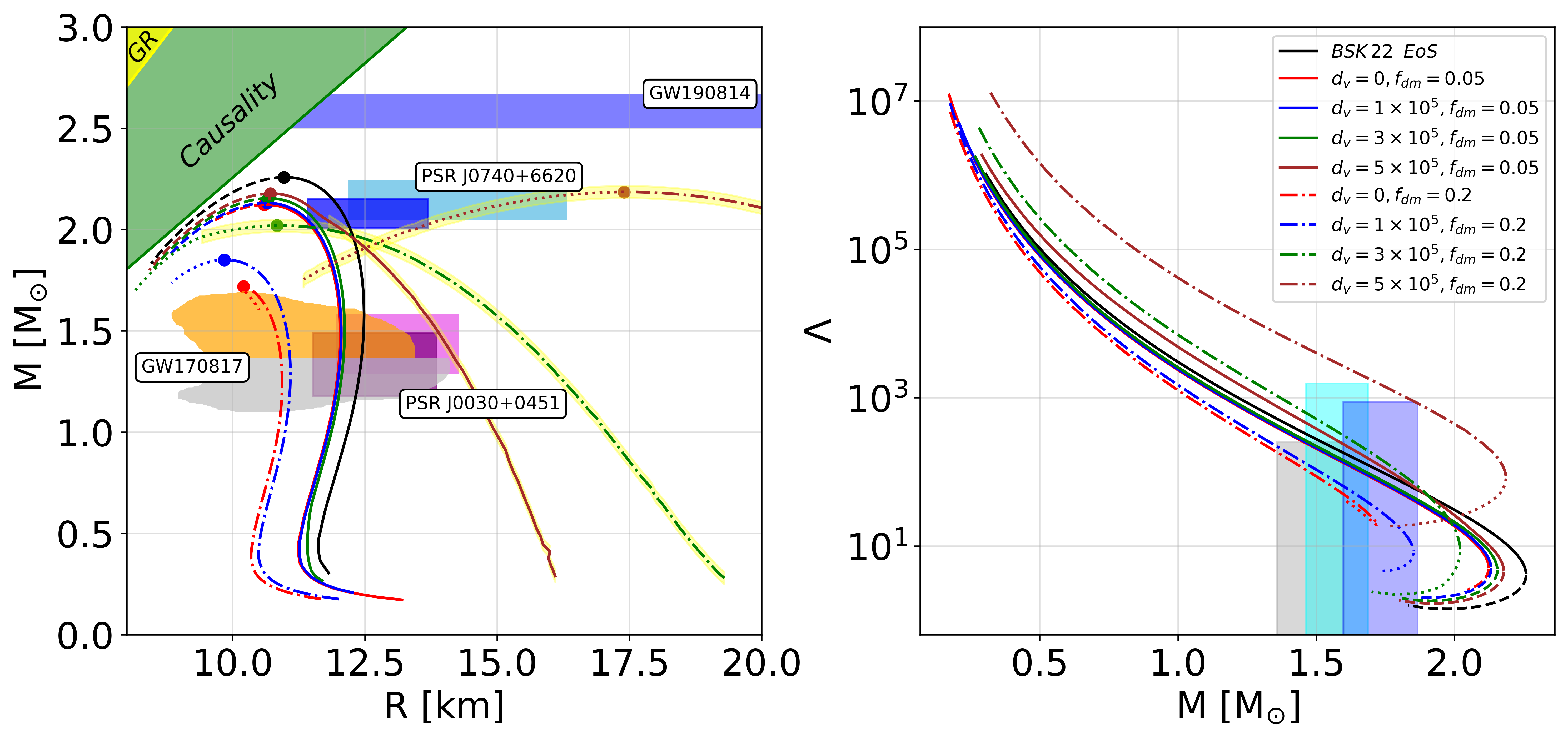
Figure 1: Mass-Radius relations (left panel) and $\Lambda$-Mass relations (right panel) for DM admixed NSs with: $M_{D}=1$ GeV, $m_{s_{1}}=10^{-14}$ eV, $m_{v}=10^{-6}$ eV, $d_{s_{1}}=10^{-4}$. We report the experimental constraints coming from the observations as well as the GR and causality bounds. The black curve corresponds to the M-R relation for BSk22 EOS, i.e. only BM ($f_{DM}=0$). The coloured curves have been obtained with different values of $d_{v}$ and DM fraction $f_{DM}=0.05$ (solid lines) and $f_{DM}=0.2$ (dash-dotted lines). These are the stable configurations. Dotted $(f_{DM}=0.2)$ and dashed lines $(f_{DM}=0.05)$ represent unstable configurations, respectively. If a point/line is highlighted in yellow, it represents a DM admixed NS with a DM halo; if not, a DM core is formed.

In FIG 1 we obtain the M-R relations by fixing $d_{s_{1}}=10^{-4}$ and considering different $d_{v}$. The value of the scalar coupling is relatively small, so that all variations with respect to the Fermi gas should be ascribed to the vector. The black solid curve represents the M-R relation for BSk22 EOS alone, namely without DM. Then we select two characteristic DM fractions: solid curves correspond to $f_{DM}=5\%$ and dash-dotted ones to $f_{DM}=20\%$. These are the stable configurations. The unstable configurations are shown with $f_{DM}=0.05$ (dashed lines) and $f_{DM}=0.2$ (dotted lines) respectively. We compare our findings with the existing theoretical/experimental constraints. In the left panel of FIG. 1, the yellow region in the upper left corner is excluded by the GR constraint $R>2GM/c^{2}$ and the green one is excluded by causality condition, $R>3GM/c^{2}$ Paerels:2009pz ; Lattimer:2012nd . Furthermore, we include the bounds on the mass and the radius obtained from the 2019 NICER data. In particular, the magenta and purple regions come from the 2019 NICER data of PSR J0030+0451 Miller:2019cac , Riley:2019yda ; the dark and light blue regions represent the 2021 NICER data with X-ray Multi-Mirror observations of PSR J0740+6620 Miller:2021qha ; Riley:2021pdl . Constraints from NS-NS merger events are also shown. The upper blue strip is from GW190814 LIGOScientific:2020zkf , while the filled orange and grey regions correspond to the estimates from GW170817 of the masses of the two NSs involved in the coalescence LIGOScientific:2018cki .

The red lines are obtained with $d_{v}=0$ and they represent a DM admixed NS where DM is basically treated as a free Fermi gas Narain:2006kx . As the DM fraction $f_{DM}$ increases, we get DM admixed NSs with smaller radii and masses. This is the typical behaviour of a DM core being accreted inside a NS Kain:2021hpk . As DM accumulates within the stellar volume, the gravitational self-attraction of the star increases. At the same time, because DM does not interact with BM, it does not significantly increase the degeneracy pressure that counteracts the contraction. Although being fermionic, the DM particles interact weakly and so they are not as densely packed as BM in NSs. The resulting degeneracy pressure adds a negligible contribution to the BM. Consequently, the outward pressure can support a lower mass, leading to DM admixed NSs that are less massive and more compact.

However, when we increase the vector coupling, the interaction strength between DM particles also increases. Eq. 22 shows that the interaction with the dark vector increases the pressure in an additive manner. This effect becomes substantial when $d_{v}$ nears $10^{5}$, which serves as a threshold value. In other words, below this threshold, there are no appreciable effects of the vector interaction. Therefore, DM admixed NS with $d_{v}=10^{5}$ (green curve) are characterized by more pressure than configurations where $d_{v}=0$ (red curves). The greater pressure manifests in a larger maximum TOV mass as well as a larger radius. Note a DM core is still formed, so the mass remains smaller than NSs without DM (black curve). This effect is barely noticeable with $f_{DM}=5$%, but it becomes more pronounced with $f_{DM}=20$ %. However, if $d_{v}$ is increased further (up to $3\times 10^{5}$), we observe much larger radii, whereas the maximum mass only increases slightly. This occurs because the DM no longer concentrates in the neutron star’s core but instead forms a halo around it Kain:2021hpk . Our DM admixed NS configurations feature a DM core if $R_{DM}<R_{BM}$; otherwise if $R_{DM}>R_{BM}$, a DM halo surrounds the star. In the left panel in FIG. 1, we highlight with a yellow shadow of the points on the M-R relations where a DM halo forms. This occurs with $d_{v}=5\times 10^{5}$ for both DM fractions and with $d_{v}=3\times 10^{5}$ at $f_{DM}=20$% (see also TABLE 1).

We find that most of the curves are compatible with the GW170817 event, and several DM-admixed NS configurations at different $f_{DM}$ values also agree with PSR J0030+0451. Interestingly, as we have shown that less massive DM admixed NSs form with an increasing DM fraction, this could potentially allow for setting constraints on the abundance and properties of DM, at least when it influences the physics of compact objects. On the other hand, PSR J0740+6620 and especially GW190814 require more mass than is likely achievable within our models.

In the right panel of FIG. 1, we present the tidal deformabilities compared with experimental constraints: the grey region represents the $90\%$ confidence upper bound from GW170817 LIGOScientific:2017vwq ; the light and dark blue regions indicate the same bounds for the primary and secondary compact objects, assuming low-spin priors for GW190425 Yang:2022ees ; LIGOScientific:2020aai . Similar to star mass, the tidal deformability also increases monotonically with a larger vector coupling. All models appear reasonable and could be constrained through NS-NS merger events.

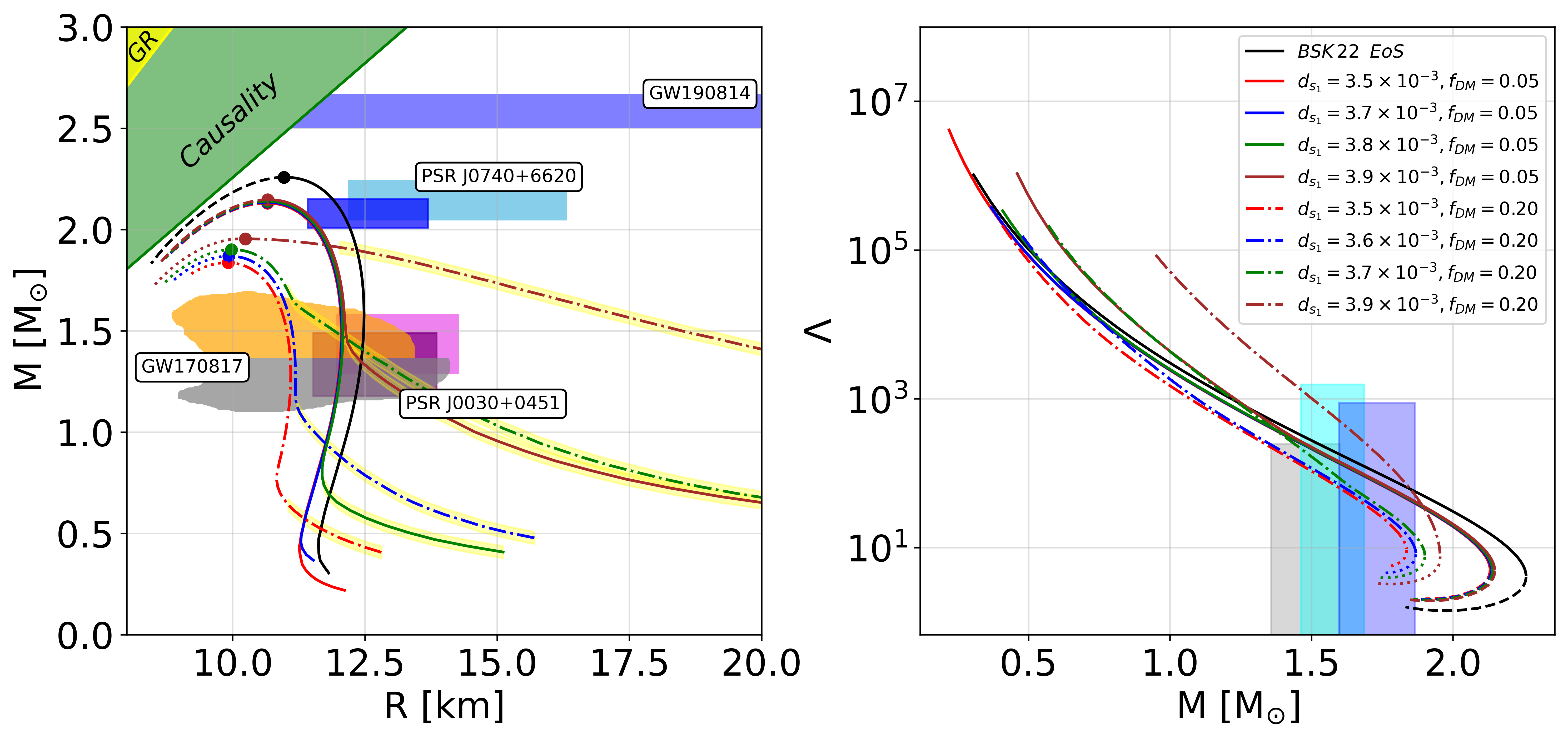
Figure 2: Mass-Radius relations (left panel) and $\Lambda$-Mass relations (right panel) for DM admixed NSs with: $M_{D}=1$ GeV, $m_{sd}=10^{-14}$ eV, $d_{v}=3\times 10^{5}$. The black curve corresponds to the M-R relation for BSk22 EOS, i.e. only BM ($f_{DM}=0$). In the right panel, the coloured curves have been obtained with different values of $d_{s_{1}}$ and $f_{DM}=0.05$ (solid lines) and $f_{DM}=0.2$ (dash-dotted lines). The yellow points and experimental constraints have the same meanings as of FIG. 1.

Having established the impact of the vector coupling, we now turn to the role of the dark scalar. In FIG. 2, we present the same M-R, $\Lambda$-M curves, this time fixing $d_{v}=3\times 10^{5}$ and varying $d_{s_{1}}$. We chose an intermediate value for $d_{v}$ (from those tested earlier) to ensure the scalar’s effects are significant. A key point in our work is that the scalar contribution becomes relevant only in combination with the vector.

In comparison with FIG 1, an even smaller variation of the coupling leads to a significant change in the M-R relations. Moreover, the stellar mass increases monotonically with increasing $d_{s_{1}}$. The similar effects of $d_{s_{1}}$ and $d_{v}$ on the DM admixed NS properties are expected because both the scalar and the vector terms in the EOS (21)-(22) have the same forms and are additive. The monotonic trend occurs because both $\epsilon$ and $P$ depend on the ratios $d_{s_{i}}/m_{i}$. In the next subsection, we show that such a behaviour does not hold when varying the self-interaction term $\lambda$ for the scalar quadratic coupling. In agreement with earlier works Nelson:2018xtr ; Kouvaris:2015rea , we find even smaller values of $d_{s_{1}}$ leave the DM settled in the core of the NS. However, here it is clear that as soon as DM forms a halo rather than a core, the mass of the DM admixed NS is not significantly affected, but the radius increases a lot. We obtain that a DM halo is not formed in only two configurations, those with relatively small couplings ($d_{s_{1}}=[3.5-3.7]\times 10^{-3}$) and $f_{DM}=5$ %. In all the other curves, there is a quite sharp transition occurring when DM is no longer confined within the stellar volume. Hence, most of the M-R relations are characterized by an evident point marking that DM extends outside the star. In other words, for these configurations the solution of the 2-fluid TOV equations (Eqs. 4 and 5) with a large central density provides a DM halo.

IV.2 Quadratic coupling

Table 2: A summary of our DM admixed NS configurations with the chosen sets of parameters for the scalar quadratic coupling scenario. From the Lagrangian in Eq. 23, $M_{D}$, $m_{s_{2}}$, $m_{v}$ represent the mass of the fermionic DM, the dark scalar mediator and the dark vector mediator, respectively. $d_{s_{2}}$, $d_{v}$ and $\lambda$ are the strength of the couplings. We report the DM fraction, the maximum mass and the corresponding radius obtained by solving the 2-fluid TOV equations (Eq. 4) and how the DM is distributed into the DM admixed NSs.

$M_{D}$ [MeV]	$m_{s_{2}}$ [keV]	$m_{v}$ [eV]	$d_{s_{2}}$	$d_{v}$	$\lambda$	Ratio	$M_{\mathrm{TOV}}$ [$M_{\odot}$]	$R_{\mathrm{TOV}}$ [km]	Dark Matter distribution
$1000$	$1$	$10^{-6}$	$10^{35}$	$3\times 10^{5}$	$5\times 10^{-2}$ $3\times 10^{-2}$ $1\times 10^{-2}$ $7\times 10^{-3}$ $5\times 10^{-3}$	$0.05$	2.1545 2.1547 2.2264 2.1396 2.1207	10.670 10.668 16.407 10.652 10.575	Core Core Halo Core Core
$1000$	$1$	$10^{-6}$	$10^{35}$	$3\times 10^{5}$	$5\times 10^{-2}$ $3\times 10^{-2}$ $1\times 10^{-2}$ $7\times 10^{-3}$ $5\times 10^{-3}$	$0.20$	2.020 2.022 2.4339 1.9139 1.7410	10.970 11.023 42.489 9.9062 9.8982	Core / Halo Core / Halo Halo Core Core
$1000$	$1$	$10^{-6}$	$1\times 10^{35}$ $3\times 10^{35}$ $5\times 10^{35}$ $7\times 10^{35}$	$3\times 10^{5}$	$5\times 10^{-2}$	$0.05$	2.1545 2.1545 2.1598 2.1750	10.670 10.662 10.706 10.722	Core Core Core / Halo Core / Halo
$1000$	$1$	$10^{-6}$	$1\times 10^{35}$ $3\times 10^{35}$ $5\times 10^{35}$ $7\times 10^{35}$	$3\times 10^{5}$	$5\times 10^{-2}$	$0.20$	2.020 2.0274 2.0592 2.1661	10.970 11.167 12.231 16.937	Core / Halo Core / Halo Core / Halo Halo

Figure 3: Mass-Radius relations (left panel) and $\Lambda$-Mass relations (right panel) for DM admixed NS with: $M_{D}=1$ GeV, $m_{s_{2}}=1$ keV, $m_{v}=10^{-6}$ eV, $d_{v}=3\times 10^{5}$, $\lambda=5\times 10^{-2}$. The black curve corresponds to the M-R relation for BSk22 EOS, i.e. only BM ($f_{DM}=0$). The coloured curves have been obtained with different values of $d_{s_{2}}$ and $f_{DM}=0.05$ (solid lines) and $f_{DM}=0.2$ (dash-dotted lines). The yellow points and experimental constraints have the same meaning of FIGs. 1 and 2.

In this Section, we examine the M-R and $\Lambda$-M relations for the scalar quadratic coupling scenario described in Section III.2.2. Similar to our approach in FIG. 2, we fix the vector coupling at $d_{v}=3\times 10^{5}$. Moreover, while in the linear scenario (Sec. III.2.1) we considered an ultralight dark scalar mediator, here we assume a massive scalar mediator with a mass of 1 keV. Indeed, a lighter scalar mediator would not significantly contribute to the scalar field expectation value (see Eq. 26). In FIG. 3, we illustrate the dependence of $d_{s_{2}}$ on the M-R and $\Lambda$-M relations. The value of $d_{s_{2}}$ can be greater than $d_{s_{1}}$ if $\phi$ respects $Z_{2}$ symmetry Banerjee:2022sqg . For a small DM fraction $(f_{DM}\sim 0.05)$ and $d_{s_{2}}\lesssim 5\times 10^{35}$, , we observe a slight increase in the radius for low-mass ($M\lesssim 1~{}M_{\odot}$) DM-admixed NS. As the scalar coupling increases further and/or more DM is accreted into the NS, a DM halo forms. Similar to the linear coupling scenario, the halo forms for comparable masses but with larger radii. Overall, the effect of $d_{s_{2}}$ is similar to that of $d_{s_{1}}$ as expected. However, a notable difference is that we do not find configurations with a DM core for $f_{DM}=20$ %. These configurations fail to meet the experimental constraints from NICER and merger events. Consequently, it appears unlikely that DM-admixed NSs can be characterized by a large DM fraction and effectively a halo if the scalar interaction is quadratic.

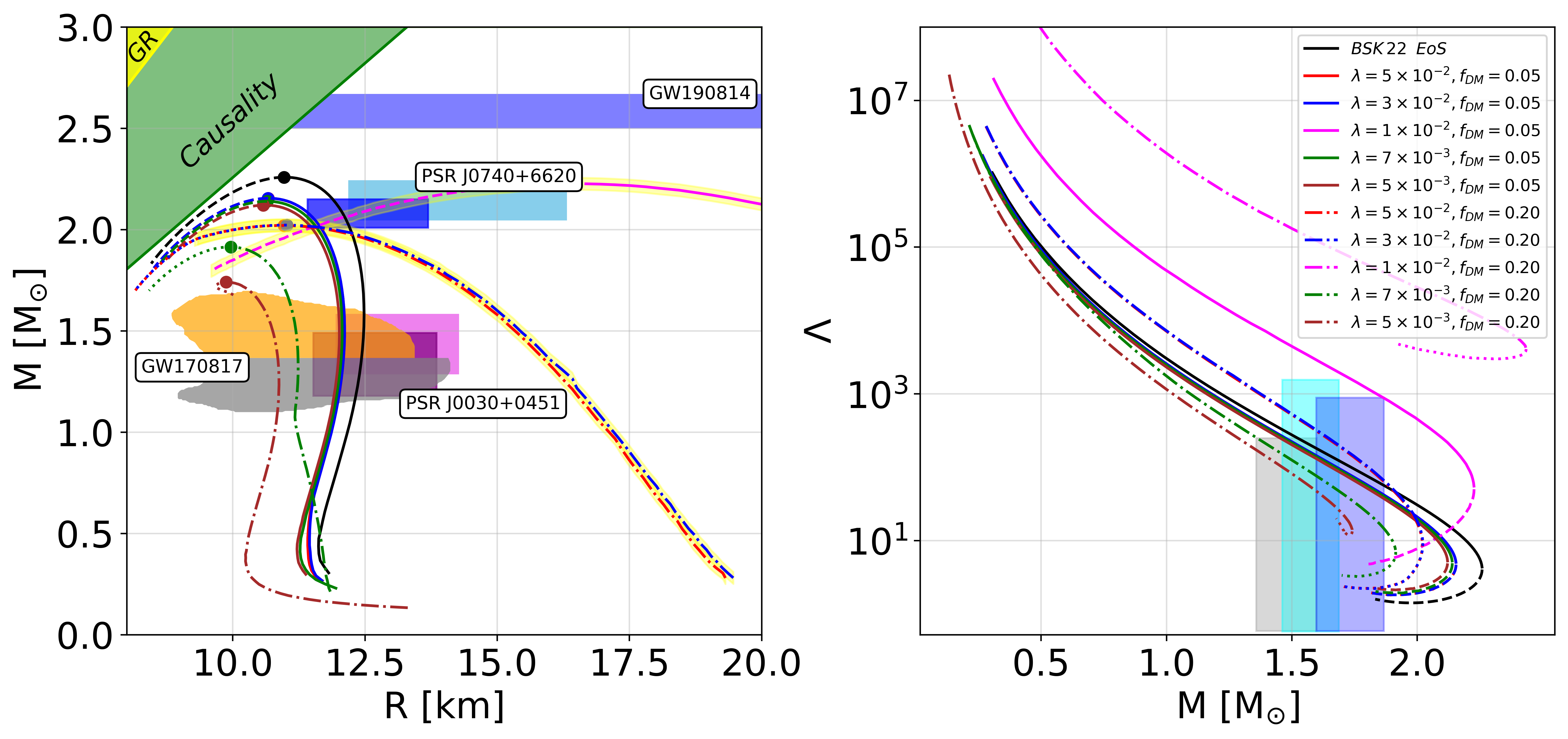
Figure 4: Mass-Radius relations (left panel) and $\Lambda$-Mass relations (right panel) for DM admixed NS with: $M_{D}=1$ GeV, $m_{s_{2}}=1$ keV, $m_{v}=10^{-6}$ eV, $d_{v}=3\times 10^{5}$, $d_{s_{2}}=1\times 10^{35}$. The black curve corresponds to the M-R relation for BSk22 EOS, i.e., only BM ($f_{DM}=0$). The coloured curves have been obtained with different values of $\lambda$ and $f_{DM}=0.05$ (solid lines) and $f_{DM}=0.2$ (dash-dotted lines). The yellow points and experimental constraints have the same meaning as of FIGs. 1 and 2

.

The Lagrangian Eq. 23 has the additional parameter $\lambda$ accounting for the quartic self-interaction. It is therefore worth investigating how it affects DM admixed NS properties. FIG. 4 shows the changes in the stellar relations with decreasing $\lambda$. The non-trivial dependence of $\lambda$ in the EOSs (Eqs. 26, 27, 28, 29) results in interesting features. For $f_{DM}=5$%, the magenta line is the only configuration where a DM halo is formed. Despite the other curves have been obtained with $\lambda>1\times 10^{-3}$ (solid red and blue) and $\lambda<1\times 10^{-3}$ (solid green and brown), none of them support halos as they almost overlap with each other. Hence, the impact of the scalar self-interaction is negligible, unless $\lambda\sim 1\times 10^{-3}$. Close to this value of $\lambda$, the energy density and the pressure (Eqs. 28 and 29) become very large, resulting in equally larger masses and radii of the corresponding DM admixed NSs. For $f_{DM}=20$%, $\lambda=5\times 10^{-2}$ provides a DM halo. The latter still forms until $\lambda$ is decreased down to $1\times 10^{-3}$. Also with $f_{DM}=20$ % we have both the M-R and $\Lambda$-M curves become very large in correspondence of $\lambda=1\times 10^{-3}$. In addition, this configuration (dash-dotted magenta line) provides $M_{TOV}=2.4339\;M_{\odot}$ and $R_{TOV}\sim 40$ km that are larger than those of BSk22 EOS alone. The off-scale value of the radius is the reason why this curve is only shown in the right panel (see TABLE 2 for details). If now $\lambda$ is decreased even more (green and brown dash-dotted curves), we obtain again configurations with smaller masses and radii. Also, a DM core is formed rather than a halo as happened for $f_{DM}=5$ %. From this discussion, we observe that increasing $\lambda$ favours the formation of a DM halo. This is similar to the effects of increasing $d_{s_{1}}$ and $d_{s_{2}}$; but we also have one crucial difference. The EOS (Eqs. 26, 27, 28, 29) in the scalar quadratic scenario longer depends only on the ratios $d_{i}/m_{i}$ (as in Eq. 12). Rather, the combination of the effects of the three couplings ($d_{v}$, $d_{s_{2}}$ and $\lambda$ in Eq. 23) is more subtle and harder to identify. This results in the fact that we observe a small interval where the effect of $\lambda$ becomes extraordinarily important. For our models, this interval is centered at $\lambda=1\times 10^{-3}$. The consequent behaviour of the mass and the radius of the DM admixed NSs in correspondence of this particular value of $\lambda$ is worth investigating further. However, it is also true it seems hard to be verified by direct observations since the resulting DM admixed NS do not fulfill the experimental constraints we select. Despite that, what we consider significant is that a similar feature may arise from a quite simple DM model when in combination with a realistic BM EOS.

V Sound speed for dark matter equation of state

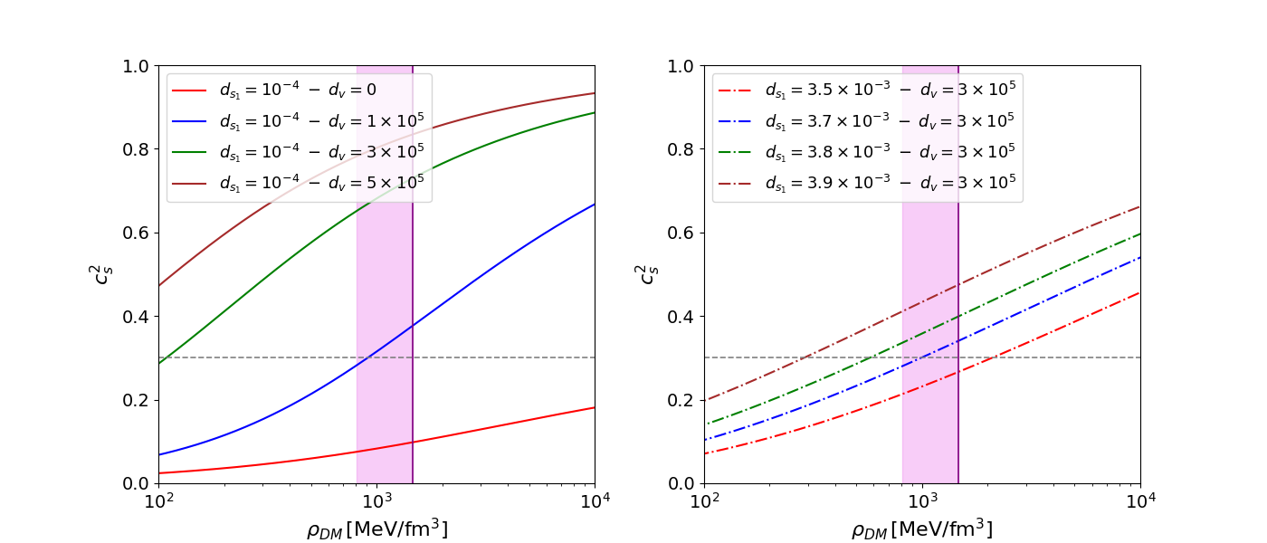
Figure 5: The sound speed $c_{s}^{2}$ as a function of energy density $\rho_{DM}$ is depicted for the scalar linear coupling scenario. The purple vertical strip represents the 95% range estimation of the larger central density inside an NS. The grey dashed line represents the conformal limit which corresponds to $c^{2}/3$. Left panel: $c_{s}^{2}$ profiles obtained by fixing all parameters but the vector coupling. The greater $d_{v}$, the larger the sound speed in the characteristic interval. Right panel: $c_{s}^{2}$ obtained by fixing all parameters but the scalar coupling. The sound speed is larger as $d_{s_{1}}$ increases but the dependence is smoother.

To characterize the DM EOS, we calculate the adiabatic sound speed Rezzolla:2013dea ; Ecker:2022xxj . The sound speed of DM at a constant entropy per baryon $S$ is expressed as

$$c_{s}^{2}:=\left(\frac{\partial P_{DM}}{\partial\rho_{DM}}\right)_{S}\,.$$ (30)

It is worth stressing that the definition 30 holds for the speed of sound within a region where only DM exists. In other words we compute $c_{s}^{2}$ of the DM fluid and not that of the whole star. Hence, we do not aim to evaluate the sound speed of the DM admixed NS. Rather, we first validate our DM EOSs by showing that they do not violate causality (i.e. $c_{s}^{2}<c^{2}(=1)$ in all our models, where $c$ is the speed of light); then we analyse the influence of the couplings $d_{v}$, $d_{s_{1}}$ and $d_{s_{2}}$ on the DM sound speed.

In FIG 5, we illustrate the variation of the sound speed with energy density for the same set of parameters used in Section IV.1. The purple band indicates the 95% confidence range for the larger central energy density inside a NS Altiparmak:2022bke . The left panel shows the dependence of $c^{2}_{s}$ on $\rho_{DM}$ for different values of $d_{v}$, while the right panel depicts similar variations for different values of $d_{s_{1}}$. Since $d_{s_{1}}$ is so small to be negligible, the red solid line (left panel) represents the sound speed for a free Fermi gas, which asymptotically approaches $1/3$ at high densities Zhou:2023ndi . When scalar and vector interactions become significant, the sound speed increases substantially beyond 1/3. This increase occurs in both panels, whether by increasing $d_{s_{1}}$ or $d_{v}$. However, the impact of $d_{v}$ on the sound speed is more pronounced, at least within the intervals considered. Even a small change in the scalar and vector couplings within these intervals results in a significant change in the sound speed.

We find that, as long as the interactions become important, $c_{s}^{2}$ consistently remains subluminar, though exceeding the QCD conformal limit $c^{2}/3$ (represented by the grey dashed line in FIG. 5) at both intermediate and large densities. The conformal limit represents the upper limit of the speed of sound inside a NS at large densities. It arises because in this regime the conformal symmetry of QCD is restored Rezzolla:2013dea . As a consequence, the sound speed approaches the value $c_{s}^{2}/3$ of conformal field theory which is realized in ultrarelativistic fluids (whose EOS takes the simplified form $P=\rho/3$). At lower densities, some works Bedaque:2014sqa ; Roy:2022nwy (and references therein) argued that the conformal limit may not be strictly valid since particles are non-relativistic. This would also be the case of cold DM. To verify whether the conformal limit holds when DM is accreted into NSs, one should compute the sound speed of the whole DM admixed NS. This will be object of our future works. Nevertheless, from the above discussion, it might be possible that in a region where only DM exists, $c_{s}^{2}$ exceeds the conformal limit. Furthermore our findings (in FIGs. 5 and 6) confirm those of Das et. al Das:2021yny and He et al. He:2022yrk , where Lagrangians similar to ours (Eqs. 12 and 23) provide sound speeds that asymptotically approach $c$ at very large densities.

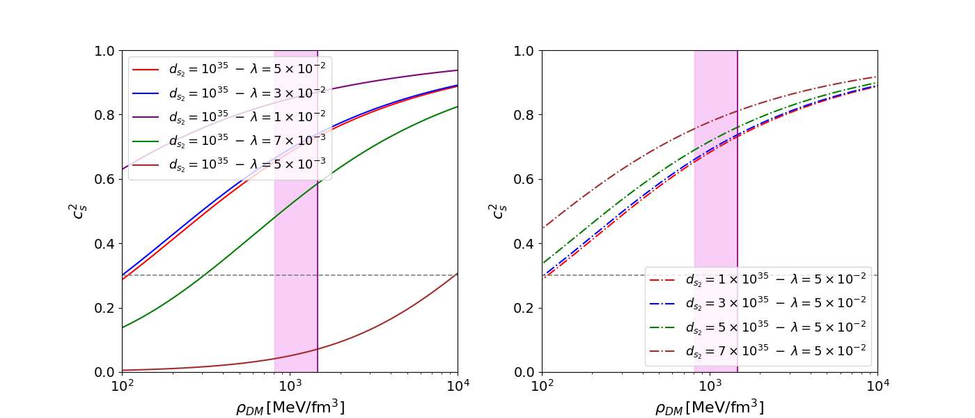
Figure 6: The sound speed $c_{s}^{2}$ as a function of energy density $\rho_{DM}$ is depicted for the scalar quadratic coupling scenario. The purple strip and grey dashed line have the same meaning as in FIG. 5. In the left panel, $c_{s}^{2}$ profiles are shown with all parameters fixed except $\lambda$. The sound speed increases as $\lambda$ decreases, reaching a peak at $\lambda=0.01$ (purple curve). For values of $\lambda$ smaller than $0.01$, $c_{s}^{2}$ starts to decrease and eventually falls below its initial value at $\lambda=0.05$. In the right panel, $c_{s}^{2}$ is displayed with all parameters fixed except $d_{s_{2}}$. The sound speed rises as the coupling $d_{s_{2}}$ increases.

The sound speed for the DM EOS in the scalar quadratic coupling scenario is shown in FIG. 6. Similar to the linear scenario, we keep the masses fixed to observe how $c_{s}^{2}$ varies with respect to $\lambda$ (left panel) and $d_{s_{2}}$ (right panel). In the right panel, we see that increasing $d_{s_{2}}$ results in a higher sound speed. The effect of the coupling $d_{s_{2}}$ is similar to that of $d_{s_{1}}$ in FIG. 5. However, the impact of $\lambda$ in the left panel is more nuanced. The sound speed increases as $\lambda$ decreases from $0.05$ to $0.01$. If $\lambda$ is reduced further, $c_{s}^{2}$ drops significantly, falling below its initial value at $\lambda=0.05$. The influence of $\lambda$ in Eqs. 26, 27, 28, 29 is complex, making the effect of the scalar self-interaction on the EOS highly dependent on the numerical values of the quartic coupling. Finally, in all models except for the brown solid curve, the sound speed exceeds $c^{2}/3$ at characteristic density regimes in NSs.

VI Conclusions and discussions

NSs serve as one of the finest astrophysical laboratories to search for DM. The direct detection of GWs from LIGO/Virgo and several X-ray spectroscopic studies of pulsars serve as a great opportunity to search for new physics. In this paper, we obtain the mass-radius and tidal deformability-mass relations of DM admixed NS, considering DM has both vector and scalar couplings. We also discuss how the stellar properties change due to the effects of linear and and quadratic dark scalar couplings with the DM fermions. We consider BSk22 EOS for modelling the baryonic sector. The DM EOS is a generalization of the free Fermi gas treatment obtained by including interactions between dark fermions with both a dark scalar and a dark vector. For the quadratic scalar coupling with the DM fermion, we need the quartic self-interaction of dark scalars to obtain realistic pressure and density for the DM sector. Depending on the coupling parameters, the DM can either form a core with a smaller effective radius or it can form a halo with a larger radius. We also derive the variations in sound speed for the DM EOS, examining the impact of vector and scalar (both linear and quadratic) couplings on the sound speed. We obtain for certain choice of DM coupling parameters, the DM sound speed exceeds the causal limit namely $c^{2}/3$, which is consistent from other existing studies, especially in the higher density environments.

In the scenario of linear coupling, when DM is accreted into a NS, the gravitational attraction increases without being balanced by additional pressure as the DM does not interact with the BM. Consequently, the higher the fraction of DM, the less massive the DM admixed NSs that form. However, with a fixed DM fraction, as one of the coupling parameters is increased, both the mass and radius of the DM admixed NSs increase monotonically. If the coupling strengths remain moderate, the DM is confined within the stellar volume, causing the DM admixed NS radius to correspond closely to that of BM, with only a slight increase.

Nevertheless, most mass-radius (M-R) curves show a point where dark matter forms a halo around the DM admixed NS instead of a core. As a result, the radius must be defined based on the halo’s extension, and the M-R curve becomes significantly smoother. This effect is more pronounced with increasing $d_{s_{1}}$, which requires a smaller change compared to $d_{v}$ to produce noticeable effects. However, the impact of scalar interaction becomes significant only when combined with the vector interaction.

For the quadratic scalar interactions, we add the quartic dark scalar self-interaction terms to obtain a self-consistent DM EOS. As anticipated, the new coupling $g_{s_{2}}$ produces a similar effect. DM admixed NSs generally have lower masses and smaller radii compared to NSs without DM. However, as $g_{s_{2}}$ is increased, both the radius and mass of the DM admixed NSs increase monotonically.

When the scalar coupling is fixed, varying $\lambda$ results in different behaviour. Specifically, the trend is no longer monotonic. Instead, the DM distribution forms a significantly extended halo as $\lambda$ initially decreases, and then becomes confined to a small core if $\lambda$ is reduced further.

The DM sound speed shows interesting behaviour for different values of linear and quadratic scalar couplings and quartic self-interactions as well. The causality condition $c_{s}^{2}<c^{2}$ is respected in all DM admixed NS configurations. This secures the consistency of our DM EOSs. In absence of the scalar, vector and quartic couplings, the sound speed reaches the conformal limit $c^{2}/3$ because the DM fluid behaves as a free Fermi gas. However, with the increase of the scalar (linear and quadratic) and vector couplings, the DM sound speed increases beyond $c^{2}/3$. However, the causal limit is not very strict at higher density and our results are consistent with other similar existing studies. The DM sound speed increases with decreasing $\lambda$. However, for $\lambda\lesssim 0.01$ the sound speed decreases further.

Our findings are consistent with the experimental bounds provided by NICER observations and detected NS merger events such as GW170817, GW190425, in terms of both M-R and $\Lambda-R$ relations. This consistency offers hope for testing and constraining new particle sector models through astrophysical observations.

References

- (1) Planck Collaboration, N. Aghanim et al., “Planck 2018 results. VI. Cosmological parameters,” Astron. Astrophys. 641 (2020) A6, arXiv:1807.06209 [astro-ph.CO]. [Erratum: Astron.Astrophys. 652, C4 (2021)].
- (2) R. Catena and P. Ullio, “A novel determination of the local dark matter density,” JCAP 08 (2010) 004, arXiv:0907.0018 [astro-ph.CO].
- (3) Y. Sofue and V. Rubin, “Rotation curves of spiral galaxies,” Ann. Rev. Astron. Astrophys. 39 (2001) 137–174, arXiv:astro-ph/0010594.
- (4) M. Markevitch, A. H. Gonzalez, D. Clowe, A. Vikhlinin, L. David, W. Forman, C. Jones, S. Murray, and W. Tucker, “Direct constraints on the dark matter self-interaction cross-section from the merging galaxy cluster 1E0657-56,” Astrophys. J. 606 (2004) 819–824, arXiv:astro-ph/0309303.
- (5) A. R. Liddle and D. H. Lyth, “The Cold dark matter density perturbation,” Phys. Rept. 231 (1993) 1–105, arXiv:astro-ph/9303019.
- (6) W. Hu, R. Barkana, and A. Gruzinov, “Cold and fuzzy dark matter,” Phys. Rev. Lett. 85 (2000) 1158–1161, arXiv:astro-ph/0003365.
- (7) L. Hui, J. P. Ostriker, S. Tremaine, and E. Witten, “Ultralight scalars as cosmological dark matter,” Phys. Rev. D 95 no. 4, (2017) 043541, arXiv:1610.08297 [astro-ph.CO].
- (8) B. Carr, F. Kuhnel, and M. Sandstad, “Primordial Black Holes as Dark Matter,” Phys. Rev. D 94 no. 8, (2016) 083504, arXiv:1607.06077 [astro-ph.CO].
- (9) J. Bramante and N. Raj, “Dark matter in compact stars,” Phys. Rept. 1052 (2024) 1–48, arXiv:2307.14435 [hep-ph].
- (10) G. G. Raffelt, Stars as laboratories for fundamental physics: The astrophysics of neutrinos, axions, and other weakly interacting particles. 5, 1996.
- (11) J. R. Oppenheimer and G. M. Volkoff, “On massive neutron cores,” Phys. Rev. 55 (1939) 374–381.
- (12) N. Rutherford, G. Raaijmakers, C. Prescod-Weinstein, and A. Watts, “Constraining bosonic asymmetric dark matter with neutron star mass-radius measurements,” Phys. Rev. D 107 no. 10, (2023) 103051, arXiv:2208.03282 [astro-ph.HE].
- (13) LIGO Scientific, Virgo Collaboration, B. P. Abbott et al., “GW170817: Observation of Gravitational Waves from a Binary Neutron Star Inspiral,” Phys. Rev. Lett. 119 no. 16, (2017) 161101, arXiv:1710.05832 [gr-qc].
- (14) LIGO Scientific, Virgo Collaboration, R. Abbott et al., “GW190814: Gravitational Waves from the Coalescence of a 23 Solar Mass Black Hole with a 2.6 Solar Mass Compact Object,” Astrophys. J. Lett. 896 no. 2, (2020) L44, arXiv:2006.12611 [astro-ph.HE].
- (15) LIGO Scientific, Virgo Collaboration, B. P. Abbott et al., “GW190425: Observation of a Compact Binary Coalescence with Total Mass ,” Astrophys. J. Lett. 892 no. 1, (2020) L3, arXiv:2001.01761 [astro-ph.HE].
- (16) M. C. Miller et al., “PSR J0030+0451 Mass and Radius from Data and Implications for the Properties of Neutron Star Matter,” Astrophys. J. Lett. 887 no. 1, (2019) L24, arXiv:1912.05705 [astro-ph.HE].
- (17) M. C. Miller et al., “The Radius of PSR J0740+6620 from NICER and XMM-Newton Data,” Astrophys. J. Lett. 918 no. 2, (2021) L28, arXiv:2105.06979 [astro-ph.HE].
- (18) T. E. Riley et al., “A View of PSR J0030+0451: Millisecond Pulsar Parameter Estimation,” Astrophys. J. Lett. 887 no. 1, (2019) L21, arXiv:1912.05702 [astro-ph.HE].
- (19) T. E. Riley et al., “A NICER View of the Massive Pulsar PSR J0740+6620 Informed by Radio Timing and XMM-Newton Spectroscopy,” Astrophys. J. Lett. 918 no. 2, (2021) L27, arXiv:2105.06980 [astro-ph.HE].
- (20) G. Raaijmakers et al., “Constraining the dense matter equation of state with joint analysis of NICER and LIGO/Virgo measurements,” Astrophys. J. Lett. 893 no. 1, (2020) L21, arXiv:1912.11031 [astro-ph.HE].
- (21) R. W. Romani, D. Kandel, A. V. Filippenko, T. G. Brink, and W. Zheng, “PSR J1810+1744: Companion Darkening and a Precise High Neutron Star Mass,” Astrophys. J. Lett. 908 no. 2, (2021) L46, arXiv:2101.09822 [astro-ph.HE].
- (22) J. Antoniadis et al., “A Massive Pulsar in a Compact Relativistic Binary,” Science 340 (2013) 6131, arXiv:1304.6875 [astro-ph.HE].
- (23) E. Fonseca et al., “Refined Mass and Geometric Measurements of the High-mass PSR J0740+6620,” Astrophys. J. Lett. 915 no. 1, (2021) L12, arXiv:2104.00880 [astro-ph.HE].
- (24) T. Binnington and E. Poisson, “Relativistic theory of tidal Love numbers,” Phys. Rev. D 80 (2009) 084018, arXiv:0906.1366 [gr-qc].
- (25) L. Rezzolla and O. Zanotti, Relativistic Hydrodynamics. Oxford University Press, 9, 2013.
- (26) J. Nättilä and J. J. E. Kajava, Fundamental physics with neutron stars. 11, 2022. arXiv:2211.15721 [astro-ph.HE].
- (27) LIGO Scientific, Virgo Collaboration, B. P. Abbott et al., “GW170817: Measurements of neutron star radii and equation of state,” Phys. Rev. Lett. 121 no. 16, (2018) 161101, arXiv:1805.11581 [gr-qc].
- (28) S. Ai, H. Gao, Y. Yuan, B. Zhang, and L. Lan, “What constraints can one pose on the maximum mass of neutron stars from multimessenger observations?,” Mon. Not. Roy. Astron. Soc. 526 no. 4, (2023) 6260–6273, arXiv:2310.07133 [astro-ph.HE].
- (29) T. Zhao and J. M. Lattimer, “Tidal Deformabilities and Neutron Star Mergers,” Phys. Rev. D 98 no. 6, (2018) 063020, arXiv:1808.02858 [astro-ph.HE].
- (30) C. Raithel, F. Özel, and D. Psaltis, “Tidal deformability from GW170817 as a direct probe of the neutron star radius,” Astrophys. J. Lett. 857 no. 2, (2018) L23, arXiv:1803.07687 [astro-ph.HE].
- (31) S. Bose, K. Chakravarti, L. Rezzolla, B. S. Sathyaprakash, and K. Takami, “Neutron-star Radius from a Population of Binary Neutron Star Mergers,” Phys. Rev. Lett. 120 no. 3, (2018) 031102, arXiv:1705.10850 [gr-qc].
- (32) L. Baiotti, “Gravitational waves from neutron star mergers and their relation to the nuclear equation of state,” Prog. Part. Nucl. Phys. 109 (2019) 103714, arXiv:1907.08534 [astro-ph.HE].
- (33) C. Kouvaris, “WIMP Annihilation and Cooling of Neutron Stars,” Phys. Rev. D 77 (2008) 023006, arXiv:0708.2362 [astro-ph].
- (34) M. A. Perez-Garcia and J. Silk, “Dark matter seeding and the kinematics and rotation of neutron stars,” Phys. Lett. B 711 (2012) 6–9, arXiv:1111.2275 [astro-ph.CO].
- (35) J. Shelton and K. M. Zurek, “Darkogenesis: A baryon asymmetry from the dark matter sector,” Phys. Rev. D 82 (2010) 123512, arXiv:1008.1997 [hep-ph].
- (36) K. Petraki and R. R. Volkas, “Review of asymmetric dark matter,” Int. J. Mod. Phys. A 28 (2013) 1330028, arXiv:1305.4939 [hep-ph].
- (37) C. Kouvaris and N. G. Nielsen, “Asymmetric Dark Matter Stars,” Phys. Rev. D 92 no. 6, (2015) 063526, arXiv:1507.00959 [hep-ph].
- (38) E. Giangrandi, V. Sagun, O. Ivanytskyi, C. Providência, and T. Dietrich, “The Effects of Self-interacting Bosonic Dark Matter on Neutron Star Properties,” Astrophys. J. 953 no. 1, (2023) 115, arXiv:2209.10905 [astro-ph.HE].
- (39) D. Rafiei Karkevandi, S. Shakeri, V. Sagun, and O. Ivanytskyi, “Tidal deformability as a probe of dark matter in neutron stars,” in 16th Marcel Grossmann Meeting on Recent Developments in Theoretical and Experimental General Relativity, Astrophysics and Relativistic Field Theories. 12, 2021. arXiv:2112.14231 [astro-ph.HE].
- (40) D. R. Karkevandi, S. Shakeri, V. Sagun, and O. Ivanytskyi, “Bosonic dark matter in neutron stars and its effect on gravitational wave signal,” Phys. Rev. D 105 no. 2, (2022) 023001, arXiv:2109.03801 [astro-ph.HE].
- (41) G. Narain, J. Schaffner-Bielich, and I. N. Mishustin, “Compact stars made of fermionic dark matter,” Phys. Rev. D 74 (2006) 063003, arXiv:astro-ph/0605724.
- (42) I. Goldman, R. N. Mohapatra, S. Nussinov, D. Rosenbaum, and V. Teplitz, “Possible Implications of Asymmetric Fermionic Dark Matter for Neutron Stars,” Phys. Lett. B 725 (2013) 200–207, arXiv:1305.6908 [astro-ph.CO].
- (43) C. Kouvaris and P. Tinyakov, “Can Neutron stars constrain Dark Matter?,” Phys. Rev. D 82 (2010) 063531, arXiv:1004.0586 [astro-ph.GA].
- (44) A. de Lavallaz and M. Fairbairn, “Neutron Stars as Dark Matter Probes,” Phys. Rev. D 81 (2010) 123521, arXiv:1004.0629 [astro-ph.GA].
- (45) M. Giannotti, I. Irastorza, J. Redondo, and A. Ringwald, “Cool WISPs for stellar cooling excesses,” JCAP 05 (2016) 057, arXiv:1512.08108 [astro-ph.HE].
- (46) A. Hook and J. Huang, “Probing axions with neutron star inspirals and other stellar processes,” JHEP 06 (2018) 036, arXiv:1708.08464 [hep-ph].
- (47) T. Kumar Poddar, S. Mohanty, and S. Jana, “Vector gauge boson radiation from compact binary systems in a gauged scenario,” Phys. Rev. D 100 no. 12, (2019) 123023, arXiv:1908.09732 [hep-ph].
- (48) T. Kumar Poddar, S. Mohanty, and S. Jana, “Constraints on ultralight axions from compact binary systems,” Phys. Rev. D 101 no. 8, (2020) 083007, arXiv:1906.00666 [hep-ph].
- (49) B. C. Seymour and K. Yagi, “Probing Massive Scalar Fields from a Pulsar in a Stellar Triple System,” Class. Quant. Grav. 37 no. 14, (2020) 145008, arXiv:1908.03353 [gr-qc].
- (50) J. A. Dror, B. V. Lehmann, H. H. Patel, and S. Profumo, “Discovering new forces with gravitational waves from supermassive black holes,” Phys. Rev. D 104 no. 8, (2021) 083021, arXiv:2105.04559 [astro-ph.CO].
- (51) G. Lambiase and T. K. Poddar, “Electrophilic scalar hair from rotating magnetized stars and effects of cosmic neutrino background,” arXiv:2404.18309 [hep-ph].
- (52) J. M. Cline and J. M. Cornell, “Dark decay of the neutron,” JHEP 07 (2018) 081, arXiv:1803.04961 [hep-ph].
- (53) W. Husain, T. F. Motta, and A. W. Thomas, “Consequences of neutron decay inside neutron stars,” JCAP 10 (2022) 028, arXiv:2203.02758 [hep-ph].
- (54) W. Husain and A. W. Thomas, “Novel neutron decay mode inside neutron stars,” J. Phys. G 50 no. 1, (2023) 015202, arXiv:2206.11262 [hep-ph].
- (55) G. F. Burgio, H. J. Schulze, I. Vidana, and J. B. Wei, “Neutron stars and the nuclear equation of state,” Prog. Part. Nucl. Phys. 120 (2021) 103879, arXiv:2105.03747 [nucl-th].
- (56) S. C. Leung, M. C. Chu, and L. M. Lin, “Dark-matter admixed neutron stars,” Phys. Rev. D 84 (2011) 107301, arXiv:1111.1787 [astro-ph.CO].
- (57) O. Ivanytskyi, V. Sagun, and I. Lopes, “Neutron stars: New constraints on asymmetric dark matter,” Phys. Rev. D 102 no. 6, (2020) 063028, arXiv:1910.09925 [astro-ph.HE].
- (58) J. Ellis, G. Hütsi, K. Kannike, L. Marzola, M. Raidal, and V. Vaskonen, “Dark Matter Effects On Neutron Star Properties,” Phys. Rev. D 97 no. 12, (2018) 123007, arXiv:1804.01418 [astro-ph.CO].
- (59) H.-M. Liu, J.-B. Wei, Z.-H. Li, G. F. Burgio, and H. J. Schulze, “Dark matter effects on the properties of neutron stars: Optical radii,” Phys. Dark Univ. 42 (2023) 101338, arXiv:2307.11313 [nucl-th].
- (60) H.-M. Liu, J.-B. Wei, Z.-H. Li, G. F. Burgio, H. C. Das, and H. J. Schulze, “Dark matter effects on the properties of neutron stars: compactness and tidal deformability,” arXiv:2403.17024 [nucl-th].
- (61) R. F. Diedrichs, N. Becker, C. Jockel, J.-E. Christian, L. Sagunski, and J. Schaffner-Bielich, “Tidal deformability of fermion-boson stars: Neutron stars admixed with ultralight dark matter,” Phys. Rev. D 108 no. 6, (2023) 064009, arXiv:2303.04089 [gr-qc].
- (62) B. Kain, “Dark matter admixed neutron stars,” Phys. Rev. D 103 no. 4, (2021) 043009, arXiv:2102.08257 [gr-qc].
- (63) Z. Rezaei, “Fuzzy dark matter in relativistic stars,” Mon. Not. Roy. Astron. Soc. 524 no. 2, (2023) 2015–2024, arXiv:2306.17665 [astro-ph.HE].
- (64) A. Das, T. Malik, and A. C. Nayak, “Dark matter admixed neutron star properties in light of gravitational wave observations: A two fluid approach,” Phys. Rev. D 105 no. 12, (2022) 123034, arXiv:2011.01318 [nucl-th].
- (65) P. Routaray, S. R. Mohanty, H. C. Das, S. Ghosh, P. J. Kalita, V. Parmar, and B. Kumar, “Investigating dark matter-admixed neutron stars with NITR equation of state in light of PSR J0952-0607,” JCAP 10 (2023) 073, arXiv:2304.05100 [nucl-th].
- (66) A. Bauswein, H. T. Janka, K. Hebeler, and A. Schwenk, “Equation-of-state dependence of the gravitational-wave signal from the ring-down phase of neutron-star mergers,” Phys. Rev. D 86 (2012) 063001, arXiv:1204.1888 [astro-ph.SR].
- (67) M. Collier, D. Croon, and R. K. Leane, “Tidal Love numbers of novel and admixed celestial objects,” Phys. Rev. D 106 no. 12, (2022) 123027, arXiv:2205.15337 [gr-qc].
- (68) T. Hinderer, “Tidal Love numbers of neutron stars,” Astrophys. J. 677 (2008) 1216–1220, arXiv:0711.2420 [astro-ph]. [Erratum: Astrophys.J. 697, 964 (2009)].
- (69) E. E. Flanagan and T. Hinderer, “Constraining neutron star tidal Love numbers with gravitational wave detectors,” Phys. Rev. D 77 (2008) 021502, arXiv:0709.1915 [astro-ph].
- (70) T. Damour and A. Nagar, “Relativistic tidal properties of neutron stars,” Phys. Rev. D 80 (2009) 084035, arXiv:0906.0096 [gr-qc].
- (71) T. Hinderer, B. D. Lackey, R. N. Lang, and J. S. Read, “Tidal deformability of neutron stars with realistic equations of state and their gravitational wave signatures in binary inspiral,” Phys. Rev. D 81 (2010) 123016, arXiv:0911.3535 [astro-ph.HE].
- (72) S. Postnikov, M. Prakash, and J. M. Lattimer, “Tidal Love Numbers of Neutron and Self-Bound Quark Stars,” Phys. Rev. D 82 (2010) 024016, arXiv:1004.5098 [astro-ph.SR].
- (73) G. F. Burgio, H.-J. Schulze, I. Vidaña, and J.-B. Wei, “A Modern View of the Equation of State in Nuclear and Neutron Star Matter,” Symmetry 13 no. 3, (2021) 400.
- (74) S. Goriely, N. Chamel, and J. M. Pearson, “Further explorations of Skyrme-Hartree-Fock-Bogoliubov mass formulas. 13. The 2012 atomic mass evaluation and the symmetry coefficient,” Phys. Rev. C 88 no. 2, (2013) 024308.
- (75) J. M. Pearson, N. Chamel, A. Y. Potekhin, A. F. Fantina, C. Ducoin, A. K. Dutta, and S. Goriely, “Unified equations of state for cold non-accreting neutron stars with Brussels–Montreal functionals – I. Role of symmetry energy,” Mon. Not. Roy. Astron. Soc. 481 no. 3, (2018) 2994–3026, arXiv:1903.04981 [astro-ph.HE]. [Erratum: Mon.Not.Roy.Astron.Soc. 486, 768 (2019)].
- (76) M. Wang, W. J. Huang, F. G. Kondev, G. Audi, and S. Naimi, “The AME 2020 atomic mass evaluation (II). Tables, graphs and references,” Chin. Phys. C 45 no. 3, (2021) 030003.
- (77) A. Y. Potekhin, A. F. Fantina, N. Chamel, J. M. Pearson, and S. Goriely, “Analytical representations of unified equations of state for neutron-star matter,” Astron. Astrophys. 560 (2013) A48, arXiv:1310.0049 [astro-ph.SR].
- (78) Q.-F. Xiang, W.-Z. Jiang, D.-R. Zhang, and R.-Y. Yang, “Effects of fermionic dark matter on properties of neutron stars,” Phys. Rev. C 89 no. 2, (2014) 025803, arXiv:1305.7354 [astro-ph.SR].
- (79) H. Shen, H. Toki, K. Oyamatsu, and K. Sumiyoshi, “Relativistic equation of state of nuclear matter for supernova and neutron star,” Nucl. Phys. A 637 (1998) 435–450, arXiv:nucl-th/9805035.
- (80) J. P. W. Diener, “Relativistic mean-field theory applied to the study of neutron star properties,” Master’s thesis, 2008.
- (81) J. Magana and T. Matos, “A brief Review of the Scalar Field Dark Matter model,” J. Phys. Conf. Ser. 378 (2012) 012012, arXiv:1201.6107 [astro-ph.CO].
- (82) P. J. E. Peebles, “Dynamics of a dark matter field with a quartic selfinteraction potential,” Phys. Rev. D 62 (2000) 023502, arXiv:astro-ph/9910350.
- (83) J. Lesgourgues, A. Arbey, and P. Salati, “A light scalar field at the origin of galaxy rotation curves,” New Astron. Rev. 46 (2002) 791–799.
- (84) A. Arbey, J. Lesgourgues, and P. Salati, “Galactic halos of fluid dark matter,” Phys. Rev. D 68 (2003) 023511, arXiv:astro-ph/0301533.
- (85) F. Paerels et al., “The Behavior of Matter under Extreme Conditions,” arXiv:0904.0435 [astro-ph.HE].
- (86) J. M. Lattimer, “The nuclear equation of state and neutron star masses,” Ann. Rev. Nucl. Part. Sci. 62 (2012) 485–515, arXiv:1305.3510 [nucl-th].
- (87) R.-X. Yang, F. Xie, and D.-J. Liu, “Tidal Deformability of Neutron Stars in Unimodular Gravity,” Universe 8 no. 11, (2022) 576, arXiv:2211.00278 [gr-qc].
- (88) A. Nelson, S. Reddy, and D. Zhou, “Dark halos around neutron stars and gravitational waves,” JCAP 07 (2019) 012, arXiv:1803.03266 [hep-ph].
- (89) A. Banerjee, G. Perez, M. Safronova, I. Savoray, and A. Shalit, “The phenomenology of quadratically coupled ultra light dark matter,” JHEP 10 (2023) 042, arXiv:2211.05174 [hep-ph].
- (90) C. Ecker and L. Rezzolla, “A General, Scale-independent Description of the Sound Speed in Neutron Stars,” Astrophys. J. Lett. 939 no. 2, (2022) L35, arXiv:2207.04417 [gr-qc].
- (91) S. Altiparmak, C. Ecker, and L. Rezzolla, “On the Sound Speed in Neutron Stars,” Astrophys. J. Lett. 939 no. 2, (2022) L34, arXiv:2203.14974 [astro-ph.HE].
- (92) D. Zhou, “Neutron Star Constraints on Neutron Dark Decays,” Universe 9 no. 11, (2023) 484.
- (93) P. Bedaque and A. W. Steiner, “Sound velocity bound and neutron stars,” Phys. Rev. Lett. 114 no. 3, (2015) 031103, arXiv:1408.5116 [nucl-th].
- (94) S. Roy and T. Suyama, “On the sound velocity bound in neutron stars,” Results Phys. 61 (2024) 107757, arXiv:2211.07874 [astro-ph.HE].
- (95) H. C. Das, A. Kumar, and S. K. Patra, “Dark matter admixed neutron star as a possible compact component in the GW190814 merger event,” Phys. Rev. D 104 no. 6, (2021) 063028, arXiv:2109.01853 [astro-ph.HE].
- (96) W.-b. He, G.-y. Shao, and C.-l. Xie, “Speed of sound and liquid-gas phase transition in nuclear matter,” Phys. Rev. C 107 no. 1, (2023) 014903, arXiv:2212.08263 [nucl-th].