Towards QCD at Five Loops

Abstract

We report on recent progress on five-loop calculations in perturbative QCD. We discuss the computation of the perturbative quark condensate, decoupling in QCD, and the precision determination of charm and bottom quark masses. For the latter, we give some first results from a gauge-invariant subset of five-loop diagrams.

1 Introduction

A cursory inspection of publications over the last two decades suggests that the first five-loop QCD calculation was completed as early as in 2005 [1], with more five-loop QCD results coming out over the following years [2, 3, 4, 5, 6, 7], culminating in a flurry of activity in 2016 and 2017 [8, 9, 10, 11, 12, 13, 14, 15, 16], and further work afterwards [17, 18]. However, a second look reveals that almost all of these works use techniques like asymptotic expansion [19, 20, 21, 22] or the R* operation [23, 24, 25, 26, 27] to reduce the number of loops to at most four. The only exception is a series of works [9, 11, 14] introducing an unphysical auxiliary mass [28, 29, 30], which means that the theory is arguably no longer QCD. It can therefore be argued that there are no genuine five-loop QCD results to date.

What could we hope to learn from a five-loop QCD calculation? The works cited above give us a first idea about the type of quantities that should be within reach soon. Order $\alpha_{s}^{5}$ corrections to the Adler function and to total hadronic decay widths, e.g. of the $\tau$ or of the Z boson, are in principle desirable for determinations of the strong coupling. However, in general better data will be needed for a significant increase in precision. Next, the energy dependence of the strong coupling and the quark masses could be determined to formally six-loop order. This would include decoupling of heavy flavours at five loops. Another example is the calculation of five-loop moments of the total cross section for heavy hadroproduction at lepton colliders, which would greatly benefit charm- and bottom quark mass determinations.

Aside from the general interest in the precise knowledge of fundamental parameters, the masses of the charm and the bottom quark have to be known with high precision for applications in flavour physics and for future Higgs coupling measurements. Projections for the HL-LHC suggest that the strength of the Yukawa coupling to the bottom quark will be measured with statistical and systematic experimental uncertainties of about one per cent [31]. At a high-energy lepton collider, the overall uncertainty could be improved by at least a factor of two and per cent level precision is within reach for the charm Yukawa coupling [32]. In order to draw conclusions about the Higgs sector, this precision has to be matched by the Standard Model prediction. This means that the bottom-quark mass has to be known to within half a per cent and the charm quark mass to within one per cent.

Whether this level of precision has already been reached with present quark mass determinations depends on the way errors are assessed and propagated when evolving the quark masses from the scale at which they are determined up to the Higgs boson mass. Following the original four-loop determination [33, 34], the perturbative uncertainty amounts to $3\,$MeV for the bottom quark and $2\,$MeV for the charm quark and is therefore negligible. However, this viewpoint has been challenged in [35, 36], where the theory uncertainties are estimated at $10\,$MeV for the bottom quark and $21\,$MeV for the charm quark. A five-loop quark mass determination would resolve this disagreement and ensure that future Higgs coupling measurements are not limited by theory.

2 Massive QCD at Five Loops

The most promising candidates for the first genuine five-loop QCD calculations are quantities depending on a single scale, which can be factored out from all Feynman integrals. If this scale is an external momentum, one arrives at massless propagator-type Feynman diagrams. For this class of diagrams, a range of dedicated methods have been developed. For example, integration-by-parts reduction can be systematised for specific diagram topologies exploiting the triangle [37] and the diamond [38] rule. Diagrams can be simplified — sometimes even reduced to trivial base cases — with the help of graphical functions [39]. Thanks to the glue-and-cut method [40], all 281 master integrals are known [41]. Still, the fact that there are 64 diagram families with 15 propagators and 20 possible scalar products poses a considerable combinatorial challenge.

An alternative is to consider problems with a single non-zero internal quark mass and vanishing external momenta. If all external particles are massless, there are 34 families of massive five-loop vacuum diagrams, with 12 propagators and 15 possible scalar products. While there are only 156 master integrals, most of them remain unknown. In the following we will focus on this scenario.

2.1 General Setup

Our calculational setup is based on the standard steps of a multiloop calculation. Diagrams are generated with QGRAF [42]. Their families are identified using custom code [43] based on nauty and Traces [44]. We use FORM [45] for inserting the Feynman rules and simplifying the resulting expressions. The resulting scalar integrals are reduced to master integrals using integration-by-parts reduction [37] via Laporta’s algorithm [46]. To this end, we use crusher [47] with tinbox [48] for reduction over finite fields [49, 50, 51, 52, 53].

2.2 The Quark Condensate

The heavy quark condensate $\langle\bar{\psi}\psi\rangle$ appears in the leading non-analytic contribution of the Operator Product Expansion [54], or equivalently, in the asymptotic small-mass expansion. It has been suggested that its non-perturbative value can be obtained from a perturbative evaluation via renormalisation group optimised perturbation theory [55, 56, 57, 58, 59]. Its anomalous dimension is proportional to the vacuum anomalous dimension $\gamma_{0}$ [60], viz.

$$\mu^{2}\frac{d}{d\mu^{2}}m\langle\bar{\psi}\psi\rangle=-4m^{4}\gamma_{0},$$ (1)

which provides a powerful cross check of the five-loop result for $\gamma_{0}$ [16].

The first two orders of the perturbative expansion of the quark condensate correspond to the sum of only two vacuum diagrams:

$$\langle\bar{\psi}\psi\rangle=\ \vbox{\hbox{\includegraphics[width=40.0pt]{qq_1L}}}\ +\ \vbox{\hbox{\includegraphics[width=40.0pt]{qq_2L}}}\ +\ \mathcal{O}(\alpha_{s}^{2}).$$ (2)

At five loops, 3451 diagrams contribute. After inserting the Feynman rules, we obtain approximately 400 000 scalar vacuum integrals with up to 4 dots (i.e. propagators raised by one power) and 4 powers of scalar products in the numerator. We consider different approaches for the numerical evaluation of the resulting 156 master integrals.

2.3 Numerical Evaluation of Master Integrals

Using FIESTA [61] for numerical sector decomposition [62], we obtain

$$\begin{split}\langle\bar{\psi}\psi\rangle\Big{|}_{\left(\frac{\alpha_{s}}{\pi}\right)^{4}}={}\frac{m^{3}}{16\pi^{2}}&\Biggl{[}\frac{(-3.5\pm 3.0)\times 10^{{-8}}}{\epsilon^{11}}+\frac{(-2.1\pm 7.6)\times 10^{{-6}}}{\epsilon^{10}}\\ &+\frac{(0.2\pm 2.1)\times 10^{{-4}}}{\epsilon^{9}}+\frac{(-0.5\pm 7.5)\times 10^{{-2}}}{\epsilon^{8}}+\mathcal{O}(\epsilon^{-7})\Biggr{]},\end{split}$$ (3)

in $d=4-2\epsilon$ dimensions, concluding that this approach alone is insufficient to obtain a meaningful result. We observe a loss of approximately two significant digits per order in the dimensional regulator $\epsilon$, which suggests that master integrals have to be known with better than double precision. We have not found any significant improvement using quasi-Monte Carlo methods [63], a quasi-finite basis [64], tropical integration [65], or pySecDec [66].

To obtain high-precision results for the master integrals, we use two approaches. In the first approach, we raise one propagator power in the master integrals to a symbolic power $x$ and obtain a coupled set of difference equations via integration-by-parts reduction. This system is solved numerically through a truncated factorial series ansatz inserting recursively determined boundary conditions for $x\to\infty$ [46, 67], where the integrals reduce to lower loops.

Alternatively, we evaluate the master integrals via numeric integration over a loop momentum, where the integrand is a propagator-type integral. It is then straightforward to evaluate the angular integral. The momentum routing can always be chosen such that the loop momentum flows through a massive line. Since all fermion lines are closed, this means that the propagator-type integrand has no massless cuts and is therefore infrared finite. Defining the loop integral measure as $[dq]\equiv\frac{d^{d}q}{i\pi^{d/2}}$, one arrives at the symbolic form

$$T=-\int_{0}^{-\infty}\frac{dq^{2}}{\Gamma(2-\epsilon)}\frac{(-q^{2})^{1-\epsilon}}{(m^{2}-q^{2})^{a}}P_{0}(q^{2})\,,$$ (4)

where $T$ denotes the original vacuum integral, $a$ the power of the propagator with momentum $q$, and $P_{0}$ the remaining propagator-type integral after removing said propagator. The integrand can be made ultraviolet finite by either introducing a suitable subtraction term or by choosing $a$ sufficiently large. In the latter case, the corresponding master integral (where typically $a=1$) can be computed from $T$ via integration-by-parts reduction.

To compute the integrand $P_{0}$ we derive a set of differential equations for the propagator-type master integrals $P_{i}$ [68, 69], which we solve for $q^{2}\to 0$ and $q^{2}\to-\infty$ with generalised power series ansätze

$$P_{i}={} \sum_{k=0}^{N-1}c_{ik}q^{2k}+\mathcal{O}(q^{2N}),$$ (5)

$$P_{i}={} \sum_{n=0}^{\#\text{loops}}\sum_{k=k_{0}}^{N-1}d_{ikn}\left(-\frac{1}{q^{2}}\right)^{k+n\epsilon}+\mathcal{O}\left(\frac{1}{(-q^{2})^{N}}\right).$$ (6)

The boundary conditions $b_{i,0}$ and $b_{i,k_{0},n}$ correspond to products of known massive vacuum diagrams [70, 71] and massless propagators [40, 72] with at most four loops. After subtracting the logarithmic high-energy contribution and performing a conformal mapping $q^{2}\to\frac{4\omega}{(1+\omega)^{2}}m^{2}$ we construct a high-precision Padé approximation from the expansion coefficients [73, 74, 75]. A similar procedure was originally proposed in [76].

As an example, we consider the following vacuum diagram, routing the numerical integration momentum through the bottom-most line:

$$\vbox{\hbox{\includegraphics[width=40.0pt]{T5L10lF12}}}=-\int\limits_{0}^{-\infty}\frac{dq^{2}}{\Gamma(2-\epsilon)}\ (-q^{2})^{1-\epsilon}\quad\vbox{\hbox{\includegraphics[width=40.0pt]{prop_orange}}}\quad\times\quad\vbox{\hbox{\includegraphics[width=80.0pt]{prop_4l}}}$$ (7)

We derive the differential equations for the four-loop propagator in the integrand and insert the ansätze in equations (5), (6). For $N=20$ we obtain the Padé approximations shown in figure 1.

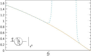
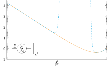
Figure 1: Padé approximations for the leading two coefficients in an expansion around $d=4$ dimensions for a four-loop propagator-type diagram.

Numerical integration then yields

$$\vbox{\hbox{\includegraphics[width=20.0pt]{T5L10lF12}}}\times e^{5\gamma_{E}\epsilon}={}5.8125309358416596949-31.572349480122869826\epsilon+\mathcal{O}(\epsilon^{2}).$$ (8)

Changing the integration contour in equation (4) to the line from $0$ to $-i\infty$ changes the result by less than $10^{-19}+2\times 10^{-18}\epsilon$. Using $N=25$ expansion terms reproduces the result within this uncertainty. We also find good agreement with a numerical evaluation using FIESTA, which yields $5.81409-31.58070(87)\epsilon$.

2.4 Decoupling

The presence of heavy quarks in virtual corrections is problematic in perturbative QCD in calculations where all other energy scales are much smaller than the heavy quark mass. On the purely practical level, diagrams with massive internal lines are notoriously hard to calculate. What is more, potentially large logarithms $\ln\frac{E}{m_{Q}}$, where $m_{Q}$ is the heavy quark mass and $E$ a typical energy for the process, can spoil the perturbative convergence in the $\overline{\text{MS}}$ scheme. The solution is to integrate out the heavy quark, i.e. to construct an effective $n_{l}$ flavour theory, where $n_{f}=n_{l}+1$ is the original number of quark flavours. The couplings can be related via

$$\alpha_{s}^{(n_{l})}=\alpha_{s}^{(n_{f})}\frac{\Delta_{cgg}}{\Pi_{c}^{2}\Pi_{g}},$$ (9)

where $\Pi_{c}$ and $\Pi_{g}$ are the (scalar) ghost and gluon polarisation functions. $\Delta_{cgg}$ is the quantum correction to the truncated 1PI ghost-gluon vertex $\Gamma_{cgg}$, viz.

$$\Gamma_{cgg}=\Gamma^{(0)}_{cgg}(1+\Delta_{cgg}),$$ (10)

where $\Gamma^{(0)}_{cgg}$ is the tree-level vertex. All Green functions are evaluated for vanishing external momentum and vanishing light quark masses. This decoupling relation is known to four-loop order [77].

At five-loop order, we obtain 131 860 803 scalar vacuum integrals with up to 7 dots and 6 scalar products. The reduction is currently ongoing, with 31 out of 34 integral families completed.

2.5 Heavy Quark Masses

The currently most precise determinations of heavy quark masses are based on sum rules. Let us define (inverse) moments $\mathcal{M}_{n}$ of the ratio $R_{Q}(s)=\frac{\sigma(e^{+}e^{-}\to Q\bar{Q})}{\sigma(e^{+}e^{-}\to\mu^{+}\mu^{-})}$ as

$$\mathcal{M}_{n}=\int^{\infty}_{s_{0}}ds\,\frac{R_{Q}(s)}{s^{n+1}}=\frac{12\pi^{2}}{n!}\left[\left(\frac{d}{dq^{2}}\right)^{n}\Pi_{Q}(q^{2})\right]_{q^{2}=0},$$ (11)

where the proportionality to a derivative of the heavy-quark contribution $\Pi_{Q}$ to the vacuum polarisation follows from a dispersion relation. These derivatives at vanishing external momentum can be evaluated perturbatively in terms of massive vacuum diagrams. The quark mass can then be extracted by comparing the calculated moments to moments obtained from the experimentally measured $R_{Q}$ ratio or moments simulated on the lattice.

We have evaluated a gauge-independent subset of the five-loop contribution to the first moment. Concretely, for $n_{h}$ degenerate massive quarks and $n_{l}$ massless quarks, we have determined the contributions proportional to $n_{h}^{4},n_{h}^{3}n_{l}$, as well as the contribution from all diagrams with two or three massless quark loops. Using the setup outlined in section 2.1 we arrive at a result expressed in terms of the master integrals depicted in figure 2.

Figure 2: Master integrals originating from vacuum diagrams with at least two massless or at least three massive quark loops.

Evaluating the master integrals with sector decomposition yields

$$\begin{split}{\cal M}_{1}^{5\text{ loop}}={}\frac{3\pi^{2}}{m_{Q}^{2}}\left(\frac{\alpha_{s}}{\pi}\right)^{4}n_{h}C_{F}\Big{[}&0.6\,T_{F}^{3}n_{l}^{3}+1.2\,T_{F}^{3}n_{l}^{2}n_{h}+0.9\,T_{F}^{3}n_{l}n_{h}^{2}\\ &+0.2\,T_{F}^{3}n_{h}^{3}+(C_{F}-5C_{A})T_{F}^{2}n_{l}^{2}+\dots\Big{]}.\end{split}$$ (12)

3 Conclusions

While there is no complete genuine five-loop QCD result so far, a number of calculations are well underway. There is steady progress towards five-loop determinations of the heavy quark condensate, the decoupling coefficients, and the masses of charm and bottom quarks from sum rules.

The biggest remaining challenge seems to be a numerical high-precision evaluation of the master integrals corresponding to massive vacuum diagrams. Here, we use a combination of sector decomposition, recurrence equations, and direct integration over one loop momentum.

References

- [1] P. A. Baikov, K. G. Chetyrkin and J. H. Kühn, Scalar correlator at O(alpha(s)**4), Higgs decay into b-quarks and bounds on the light quark masses, Phys. Rev. Lett. 96 (2006) 012003 [hep-ph/0511063].
- [2] M. Schreck and M. Steinhauser, Higgs Decay to Gluons at NNLO, Phys. Lett. B 655 (2007) 148 [0708.0916].
- [3] P. A. Baikov, K. G. Chetyrkin and J. H. Kühn, Order alpha**4(s) QCD Corrections to Z and tau Decays, Phys. Rev. Lett. 101 (2008) 012002 [0801.1821].
- [4] P. A. Baikov, K. G. Chetyrkin and J. H. Kühn, Adler Function, Bjorken Sum Rule, and the Crewther Relation to Order in a General Gauge Theory, Phys. Rev. Lett. 104 (2010) 132004 [1001.3606].
- [5] P. A. Baikov, K. G. Chetyrkin, J. H. Kühn and J. Rittinger, Complete QCD Corrections to Hadronic -Decays, Phys. Rev. Lett. 108 (2012) 222003 [1201.5804].
- [6] P. A. Baikov, K. G. Chetyrkin, J. H. Kühn and J. Rittinger, Adler Function, Sum Rules and Crewther Relation of Order : the Singlet Case, Phys. Lett. B 714 (2012) 62 [1206.1288].
- [7] P. A. Baikov, K. G. Chetyrkin and J. H. Kühn, Quark Mass and Field Anomalous Dimensions to , JHEP 10 (2014) 076 [1402.6611].
- [8] P. A. Baikov, K. G. Chetyrkin and J. H. Kühn, Five-Loop Running of the QCD coupling constant, Phys. Rev. Lett. 118 (2017) 082002 [1606.08659].
- [9] T. Luthe, A. Maier, P. Marquard and Y. Schröder, Five-loop quark mass and field anomalous dimensions for a general gauge group, JHEP 01 (2017) 081 [1612.05512].
- [10] F. Herzog, B. Ruijl, T. Ueda, J. A. M. Vermaseren and A. Vogt, The five-loop beta function of Yang-Mills theory with fermions, JHEP 02 (2017) 090 [1701.01404].
- [11] T. Luthe, A. Maier, P. Marquard and Y. Schröder, Complete renormalization of QCD at five loops, JHEP 03 (2017) 020 [1701.07068].
- [12] P. A. Baikov, K. G. Chetyrkin and J. H. Kühn, Five-loop fermion anomalous dimension for a general gauge group from four-loop massless propagators, JHEP 04 (2017) 119 [1702.01458].
- [13] F. Herzog, B. Ruijl, T. Ueda, J. A. M. Vermaseren and A. Vogt, On Higgs decays to hadrons and the R-ratio at N4LO, JHEP 08 (2017) 113 [1707.01044].
- [14] T. Luthe, A. Maier, P. Marquard and Y. Schröder, The five-loop Beta function for a general gauge group and anomalous dimensions beyond Feynman gauge, JHEP 10 (2017) 166 [1709.07718].
- [15] K. G. Chetyrkin, G. Falcioni, F. Herzog and J. A. M. Vermaseren, Five-loop renormalisation of QCD in covariant gauges, JHEP 10 (2017) 179 [1709.08541].
- [16] P. A. Baikov and K. G. Chetyrkin, QCD vacuum energy in 5 loops, PoS RADCOR2017 (2018) 025.
- [17] F. Herzog, S. Moch, B. Ruijl, T. Ueda, J. A. M. Vermaseren and A. Vogt, Five-loop contributions to low-N non-singlet anomalous dimensions in QCD, Phys. Lett. B 790 (2019) 436 [1812.11818].
- [18] M. Fael, K. Schönwald and M. Steinhauser, A first glance to the kinematic moments of B → Xc at third order, JHEP 08 (2022) 039 [2205.03410].
- [19] K. G. Chetyrkin, Operator Expansions in the Minimal Subtraction Scheme. 1: The Gluing Method, Theor. Math. Phys. 75 (1988) 346.
- [20] K. G. Chetyrkin, Operator Expansions in the Minimal Subtraction Scheme. 2: Explicit Formulas for Coefficient Functions, Theor. Math. Phys. 76 (1988) 809.
- [21] V. A. Smirnov, Asymptotic expansions in limits of large momenta and masses, Commun. Math. Phys. 134 (1990) 109.
- [22] M. Beneke and V. A. Smirnov, Asymptotic expansion of Feynman integrals near threshold, Nucl. Phys. B 522 (1998) 321 [hep-ph/9711391].
- [23] K. G. Chetyrkin and F. V. Tkachov, Infrared r operation and ultraviolet counterterms in the ms scheme, Phys. Lett. B 114 (1982) 340.
- [24] K. G. Chetyrkin and V. A. Smirnov, R* operation corrected, Phys. Lett. B 144 (1984) 419.
- [25] V. A. Smirnov and K. G. Chetyrkin, R* Operation in the Minimal Subtraction Scheme, Theor. Math. Phys. 63 (1985) 462.
- [26] K. G. Chetyrkin, Combinatorics of -, -, and -operations and asymptotic expansions of feynman integrals in the limit of large momenta and masses, 1701.08627.
- [27] F. Herzog and B. Ruijl, The R∗-operation for Feynman graphs with generic numerators, JHEP 05 (2017) 037 [1703.03776].
- [28] M. Misiak and M. Münz, Two loop mixing of dimension five flavor changing operators, Phys. Lett. B 344 (1995) 308 [hep-ph/9409454].
- [29] T. van Ritbergen, J. A. M. Vermaseren and S. A. Larin, The Four loop beta function in quantum chromodynamics, Phys. Lett. B 400 (1997) 379 [hep-ph/9701390].
- [30] K. G. Chetyrkin, M. Misiak and M. Münz, Beta functions and anomalous dimensions up to three loops, Nucl. Phys. B 518 (1998) 473 [hep-ph/9711266].
- [31] M. Cepeda et al., Report from Working Group 2: Higgs Physics at the HL-LHC and HE-LHC, CERN Yellow Rep. Monogr. 7 (2019) 221 [1902.00134].
- [32] K. Fujii et al., Physics Case for the International Linear Collider, 1506.05992.
- [33] K. G. Chetyrkin, J. H. Kühn, A. Maier, P. Maierhöfer, P. Marquard, M. Steinhauser et al., Charm and Bottom Quark Masses: An Update, Phys. Rev. D 80 (2009) 074010 [0907.2110].
- [34] K. G. Chetyrkin, J. H. Kühn, A. Maier, P. Maierhöfer, P. Marquard, M. Steinhauser et al., Addendum to “Charm and bottom quark masses: An update”, 1710.04249.
- [35] B. Dehnadi, A. H. Hoang, V. Mateu and S. M. Zebarjad, Charm Mass Determination from QCD Charmonium Sum Rules at Order , JHEP 09 (2013) 103 [1102.2264].
- [36] B. Dehnadi, A. H. Hoang and V. Mateu, Bottom and Charm Mass Determinations with a Convergence Test, JHEP 08 (2015) 155 [1504.07638].
- [37] K. G. Chetyrkin and F. V. Tkachov, Integration by parts: The algorithm to calculate -functions in 4 loops, Nucl. Phys. B 192 (1981) 159.
- [38] B. Ruijl, T. Ueda and J. Vermaseren, The diamond rule for multi-loop Feynman diagrams, Phys. Lett. B 746 (2015) 347 [1504.08258].
- [39] O. Schnetz, Graphical functions and single-valued multiple polylogarithms, Commun. Num. Theor. Phys. 08 (2014) 589 [1302.6445].
- [40] P. A. Baikov and K. G. Chetyrkin, Four Loop Massless Propagators: An Algebraic Evaluation of All Master Integrals, Nucl. Phys. B 837 (2010) 186 [1004.1153].
- [41] A. Georgoudis, V. Gonçalves, E. Panzer, R. Pereira, A. V. Smirnov and V. A. Smirnov, Glue-and-cut at five loops, JHEP 09 (2021) 098 [2104.08272].
- [42] P. Nogueira, Automatic Feynman graph generation, J. Comput. Phys. 105 (1993) 279.
- [43] A. Maier, dynast. https://github.com/a-maier/dynast.
- [44] B. D. McKay and A. Piperno, Practical graph isomorphism, ii, Journal of Symbolic Computation 60 (2014) 94 [1301.1493].
- [45] J. A. M. Vermaseren, New features of FORM, math-ph/0010025.
- [46] S. Laporta, High precision calculation of multiloop Feynman integrals by difference equations, Int. J. Mod. Phys. A15 (2000) 5087 [hep-ph/0102033].
- [47] P. Marquard and D. Seidel, The IBP package Crusher. Unpublished.
- [48] A. Maier and P. Marquard, tinbox, a finite field solver. Unpublished.
- [49] M. Kauers, Fast solvers for dense linear systems, Nucl. Phys. B Proc. Suppl. 183 (2008) 245.
- [50] P. Kant, Finding Linear Dependencies in Integration-By-Parts Equations: A Monte Carlo Approach, Comput. Phys. Commun. 185 (2014) 1473 [1309.7287].
- [51] A. von Manteuffel and R. M. Schabinger, A novel approach to integration by parts reduction, Phys. Lett. B 744 (2015) 101 [1406.4513].
- [52] T. Peraro, Scattering amplitudes over finite fields and multivariate functional reconstruction, JHEP 12 (2016) 030 [1608.01902].
- [53] J. Klappert and F. Lange, Reconstructing rational functions with FireFly, Comput. Phys. Commun. 247 (2020) 106951 [1904.00009].
- [54] K. G. Wilson, Nonlagrangian models of current algebra, Phys. Rev. 179 (1969) 1499.
- [55] J. L. Kneur and A. Neveu, Renormalization Group Improved Optimized Perturbation Theory: Revisiting the Mass Gap of the O(2N) Gross-Neveu Model, Phys. Rev. D 81 (2010) 125012 [1004.4834].
- [56] J. L. Kneur and A. Neveu, from Renormalization Group Optimized Perturbation, Phys. Rev. D 85 (2012) 014005 [1108.3501].
- [57] J.-L. Kneur and A. Neveu, from and Renormalization Group Optimized Perturbation Theory, Phys. Rev. D 88 (2013) 074025 [1305.6910].
- [58] J.-L. Kneur and A. Neveu, Chiral condensate from renormalization group optimized perturbation, Phys. Rev. D 92 (2015) 074027 [1506.07506].
- [59] J.-L. Kneur and A. Neveu, Chiral condensate and spectral density at full five-loop and partial six-loop orders of renormalization group optimized perturbation theory, Phys. Rev. D 101 (2020) 074009 [2001.11670].
- [60] V. P. Spiridonov and K. G. Chetyrkin, Nonleading mass corrections and renormalization of the operators m psi-bar psi and g**2(mu nu), Sov. J. Nucl. Phys. 47 (1988) 522.
- [61] A. V. Smirnov, N. D. Shapurov and L. I. Vysotsky, FIESTA5: Numerical high-performance Feynman integral evaluation, Comput. Phys. Commun. 277 (2022) 108386 [2110.11660].
- [62] T. Binoth and G. Heinrich, An automatized algorithm to compute infrared divergent multiloop integrals, Nucl. Phys. B 585 (2000) 741 [hep-ph/0004013].
- [63] S. Borowka, G. Heinrich, S. Jahn, S. P. Jones, M. Kerner and J. Schlenk, A GPU compatible quasi-Monte Carlo integrator interfaced to pySecDec, Comput. Phys. Commun. 240 (2019) 120 [1811.11720].
- [64] A. von Manteuffel, E. Panzer and R. M. Schabinger, A quasi-finite basis for multi-loop Feynman integrals, JHEP 02 (2015) 120 [1411.7392].
- [65] M. Borinsky, Tropical Monte Carlo quadrature for Feynman integrals, Ann. Inst. H. Poincare D Comb. Phys. Interact. 10 (2023) 635 [2008.12310].
- [66] G. Heinrich, S. P. Jones, M. Kerner, V. Magerya, A. Olsson and J. Schlenk, Numerical scattering amplitudes with pySecDec, Comput. Phys. Commun. 295 (2024) 108956 [2305.19768].
- [67] T. Luthe and Y. Schröder, Fun with higher-loop Feynman diagrams, J. Phys. Conf. Ser. 762 (2016) 012066 [1604.01262].
- [68] A. V. Kotikov, Differential equations method: New technique for massive Feynman diagrams calculation, Phys. Lett. B 254 (1991) 158.
- [69] E. Remiddi, Differential equations for Feynman graph amplitudes, Nuovo Cim. A 110 (1997) 1435 [hep-th/9711188].
- [70] Y. Schröder and A. Vuorinen, High-precision epsilon expansions of single-mass-scale four-loop vacuum bubbles, JHEP 06 (2005) 051 [hep-ph/0503209].
- [71] K. G. Chetyrkin, M. Faisst, J. H. Kühn, P. Maierhöfer and C. Sturm, Four-Loop QCD Corrections to the Rho Parameter, Phys. Rev. Lett. 97 (2006) 102003 [hep-ph/0605201].
- [72] R. N. Lee, A. V. Smirnov and V. A. Smirnov, Master Integrals for Four-Loop Massless Propagators up to Transcendentality Weight Twelve, Nucl. Phys. B 856 (2012) 95 [1108.0732].
- [73] P. A. Baikov and D. J. Broadhurst, Three loop QED vacuum polarization and the four loop muon anomalous magnetic moment, in 4th International Workshop on Software Engineering and Artificial Intelligence for High-energy and Nuclear Physics, 4, 1995, hep-ph/9504398.
- [74] P. A. Baikov, A. Maier and P. Marquard, The QED vacuum polarization function at four loops and the anomalous magnetic moment at five loops, Nucl. Phys. B 877 (2013) 647 [1307.6105].
- [75] A. Maier and P. Marquard, Life of , Phys. Rev. D 97 (2018) 056016 [1710.03724].
- [76] M. Faisst, K. G. Chetyrkin and J. H. Kühn, Multiloop tadpoles, Nucl. Phys. B Proc. Suppl. 135 (2004) 307.
- [77] Y. Schröder and M. Steinhauser, Four-loop decoupling relations for the strong coupling, JHEP 01 (2006) 051 [hep-ph/0512058].