1]\orgdivElectrical and Computer Engineering Department, \orgnameUniversity of California, Los Angeles, \orgaddress\street420 Westwood Plaza, \cityLos Angeles, \postcode90095, \stateCA, \countryUnited States
Nonlinear Schrödinger Network
Abstract
Deep neural networks (DNNs) have achieved exceptional performance across various fields by learning complex nonlinear mappings from large-scale datasets. However, they encounter challenges such as high computational costs and limited interpretability. To address these issues, hybrid approaches that integrate physics with AI are gaining interest. This paper introduces a novel physics-based AI model called the “Nonlinear Schrödinger Network”, which treats the Nonlinear Schrödinger Equation (NLSE) as a general-purpose trainable model for learning complex patterns including nonlinear mappings and memory effects from data. Existing physics-informed machine learning methods use neural networks to approximate the solutions of partial differential equations (PDEs). In contrast, our approach directly treats the PDE as a trainable model to obtain general nonlinear mappings that would otherwise require neural networks. As a type of physics-AI symbiosis, it offers a more interpretable and parameter-efficient alternative to traditional black-box neural networks, achieving comparable or better accuracy in some time series classification tasks while significantly reducing the number of required parameters. Notably, the trained Nonlinear Schrödinger Network is interpretable, with all parameters having physical meanings as properties of a virtual physical system that transforms the data to a more separable space. This interpretability allows for insight into the underlying dynamics of the data transformation process. Applications to time series forecasting have also been explored. While our current implementation utilizes the NLSE, the proposed method of using physics equations as trainable models to learn nonlinear mappings from data is not limited to the NLSE and may be extended to other master equations of physics.
1 Introduction
Deep neural networks (DNNs) have emerged as a powerful tool for learning complex nonlinear mappings from data, achieving state-of-the-art performance in various fields including computer vision, natural language processing, and scientific computing. By leveraging their deep hierarchical structure along with billions or even trillions of trainable parameters, DNNs have demonstrated remarkable capability to learn complex patterns from vast amounts of data. However, the success of DNNs comes with challenges, such as the reliance on large-scale datasets, high computational and memory costs, and limited interpretability. To address these challenges, there is a growing interest in hybrid approaches that integrate physics with AI to enable better inference, prediction, vision, control and more [1, 2]. For example, physical principles can be leveraged as prior knowledge to design neural networks with special architectures and loss functions, enabling more efficient modeling of complex physical systems [3, 4]. Moreover, physical systems can act as analog computers to perform specialized computations or transform the data in a manner that reduces the burden on digital processors [5, 6, 7].
One example from our own work is the nonlinear Schrödinger kernel [7], a hardware acceleration technique that was originally proposed to bridge the latency gap between ultrafast data acquisition in optical systems and neural network inference on digital computers. The nonlinear Schrödinger kernel operates by modulating the input data onto the spectrum of a femtosecond laser pulse and then propagating the pulse through a nonlinear optical medium, where complex nonlinear interactions governed by the Nonlinear Schrödinger Equation (NLSE) lead to a transformation of the data that makes it more separable by a simple linear classifier. Notably, operating in the optical domain reduces latency by orders of magnitude compared to utilizing numerical kernels like radius basis function (RBF). The benefits are gained without an increase of data dimensionality. Our follow-up work has demonstrated that while the nonlinear optical system cannot be directly tuned, the nonlinear transformation can be effectively engineered by varying the phase of the input data via spectral phase encoding with an optimization feedback loop [8]. This further improves the performance and generalization of the nonlinear Schrödinger kernel.
While the nonlinear Schrödinger kernel technique has shown promising results in terms of classification accuracy and speed, its physical implementation presents certain limitations, such as the fixed nature of a given optical medium and the need for specialized hardware. However, its underlying principles, particularly the use of nonlinear transformation stemming from the Nonlinear Schrödinger Equation (NLSE) to improve data separability, can potentially be adapted to fully digital algorithms. In this paper, we propose the “Nonlinear Schrödinger Network”, a novel physics-inspired trainable model that operates entirely in the digital domain. This approach treats the NLSE as a trainable model to learn the complex patterns from data. By optimizing the coefficients of the NLSE using backpropagation and stochastic gradient descent (SGD), nonlinear mappings can be learned to transform the data adaptively for classification tasks. Unlike existing work on using neural networks to approximate the solution of a partial differential equation (PDE) [3, 4], our proposed approach directly learns the coefficients of the PDE itself to obtain general nonlinear mappings that would otherwise require neural networks. This physics-inspired approach provides a more interpretable and parameter-efficient model compared to black-box neural networks. By leveraging the low-dimensional nature of physical laws, the Nonlinear Schrödinger Network represents complex data transformations with significantly fewer parameters while achieving accuracy comparable to traditional neural networks on nonlinear classification tasks.
2 Related Work
2.1 Nonlinear Schrödinger Kernel Computing
Despite the increasing speed of digital processors, the execution time of AI algorithms are still orders of magnitude slower than the time scales in ultrafast optical imaging, sensing, and metrology. To address this problem, a new concept in hardware acceleration of AI that exploits femtosecond pulses for both data acquisition and computing called nonlinear Schrödinger kernel has been demonstrated [7]. This method modulates data onto a supercontinuum laser spectrum, which then undergoes a nonlinear optical transformation analogous to a kernel operation, enhancing data classification accuracy. It is shown that the nonlinear optical kernel can improve the linear classification results similar to a traditional numerical kernel (such as the radial-basis-function (RBF)) but with orders of magnitude lower latency. The inference latency of the RBF kernel with a linear classifier is on the order of to second, while the nonlinear Schrödinger kernel achieves a substantially reduced latency on the order of second and better classification accuracy. In the original work [7], the performance is data-dependent due to the limited degrees of freedom and the unsupervised nature of the optical kernel. The follow-up work has demonstrated that by modulating the spectral phase of the input data, the nonlinear optical interactions within the kernel can be effectively engineered [8]. Incorporating this phase encoding scheme within a digital optimization feedback loop allows the optical kernel to be trained in a data-driven manner, minimizing the classification error of the digital backend.
2.2 Neural Networks as PDE Solvers
An emerging trend in blending physics and AI is the use of neural networks as computationally efficient surrogates for solving partial differential equations (PDEs). This approach has the potential to significantly accelerate forward simulations and inverse design used in the optimization of engineered physical systems. For example, neural networks can compute the transmission spectra of metasurfaces orders of magnitude faster than numerically solving the full Maxwell’s equations [9, 10]. Similarly, neural networks trained on real-world data can model intricate fluid flows for applications like weather forecasting and aerodynamics, circumventing the need to directly solve the Navier-Stokes equations [11]. More ambitious attempts have been made to develop general neural network architectures that can learn different types of PDEs. Physics-informed neural network (PINN) [3] is a pioneering example which utilizes a physics-driven loss derived from the equation itself to solve one instance of the PDE with a fixed set of parameters and conditions. Fourier Neural Operator (FNO) [4] takes a step further by learning the nonlinear mapping of an entire family of PDEs.
3 Nonlinear Schrödinger Network
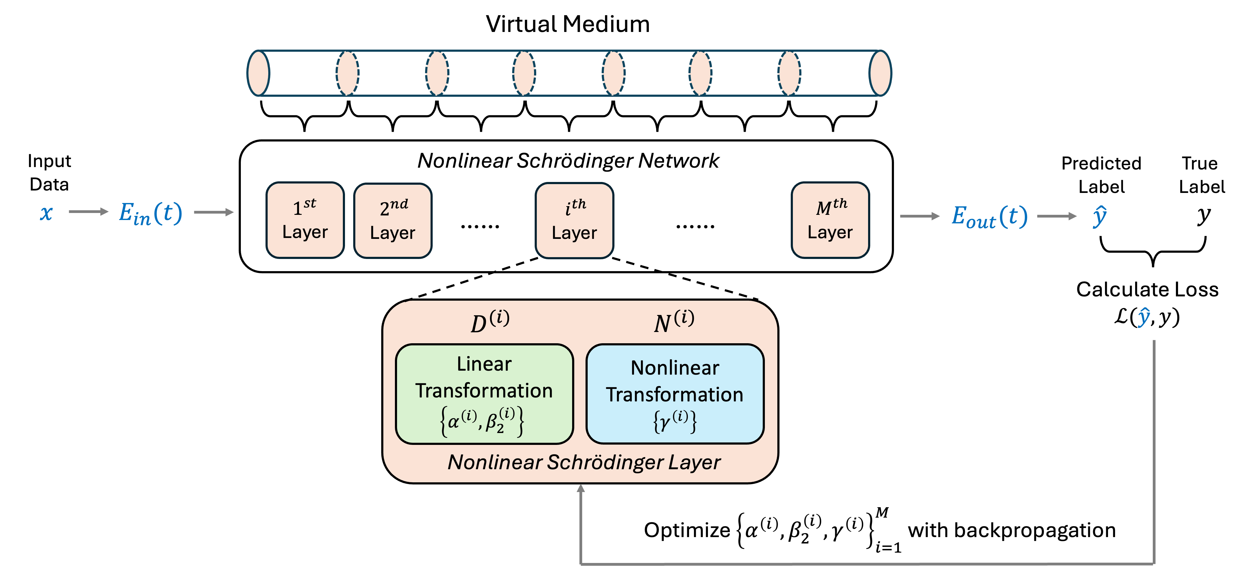
The Nonlinear Schrödinger Equation (NLSE) is one of the canonical equations of physics, accounting for three primary effects: attenuation, dispersion, and nonlinearity. These effects, in the limit of constant group delay dispersion (GDD), are represented by parameters , , and , respectively, as illustrated in Equation 1. The NLSE has demonstrated significant success in describing systems with complex memory and nonlinear effects. In this paper, we treat the NLSE as a trainable model by dividing a virtual medium it into layers, wherein each layer has learnable nonlinear and dispersive properties that can be trained with backpropagation and gradient descent.
| (1) |

Figure 1 presents a schematic diagram of the Nonlinear Schrödinger Network, a novel physics-inspired trainable model. The input data is treated as an input that propagates through a virtual medium, wherein the propagation over a short distance is represented by a Nonlinear Schrödinger Layer with two main components: a linear transformation parameterized by and , followed by a nonlinear transformation parameterized by , as described below.
| (2) |
| (3) |
This structure resembles a single block in a common neural network, where a linear layer is typically followed by a nonlinear activation function. By cascading several Nonlinear Schrödinger Layers, we construct a “Nonlinear Schrödinger Network”, a model capable of learning nonlinear mappings from the input data to the desired output.
In Equation 2 and 3, is a 1D vector with being its corresponding frequency vector. , , and are trainable scalars in each layer, and is a constant scalar. and represent 1D Fourier transform and 1D inverse Fourier transform, respectively. As the input data traverses the layers, it undergoes a series of transformations governed by the NLSE, resulting in the transformed output . Such an output is then mapped to the predicted label , which is compared with the true label to compute the loss . With all the operations being differentiable, backpropagation and stochastic gradient descent are utilized to update the trainable parameters across all the layers.
Remarkably, each Nonlinear Schrödinger Layer only introduces three trainable parameters, yet they can parameterize the nonlinear transformation more efficiently than conventional neural networks, as demonstrated later in this work. Moreover, since the trainable parameters are coefficients of a physics equation, the resulting model is interpretable by the physics. This unique property distinguishes the Nonlinear Schrödinger Network from traditional black-box neural networks.
It is worth noting that we modulate the original 1D data onto a super-Gaussian pulse with zero padding for more accurate spectral representations during the computation [12]. The computation across all the Nonlinear Schrödinger Layers doesn’t change the dimension of data, and the desired output may have different dimensions compared to , especially in classification tasks. To align with the output dimension, a densely connected linear layer will be added.
4 Results
4.1 Time Series Classification
We demonstrate the performance of the proposed Nonlinear Schrödinger Network on three time series classification datasets from different domains and compare it with conventional neural networks.
-
•
Ford Engine Dataset [13]: This dataset consists of time series representing measurements of engine noise. The classification problem is to diagnose whether a specific symptom exists or not in an automotive subsystem, which is a binary classification task.
-
•
Starlight Curve Dataset [14]: Each time series in this dataset records the brightness of a celestial object as a function of time. The classification task is to associate the light curves with three different sources.
-
•
Spoken Digits Dataset [15]: This dataset contains recordings of digits (0-9) at 8kHz from different speakers. The classification task is to classify the recording as one of the ten digits.
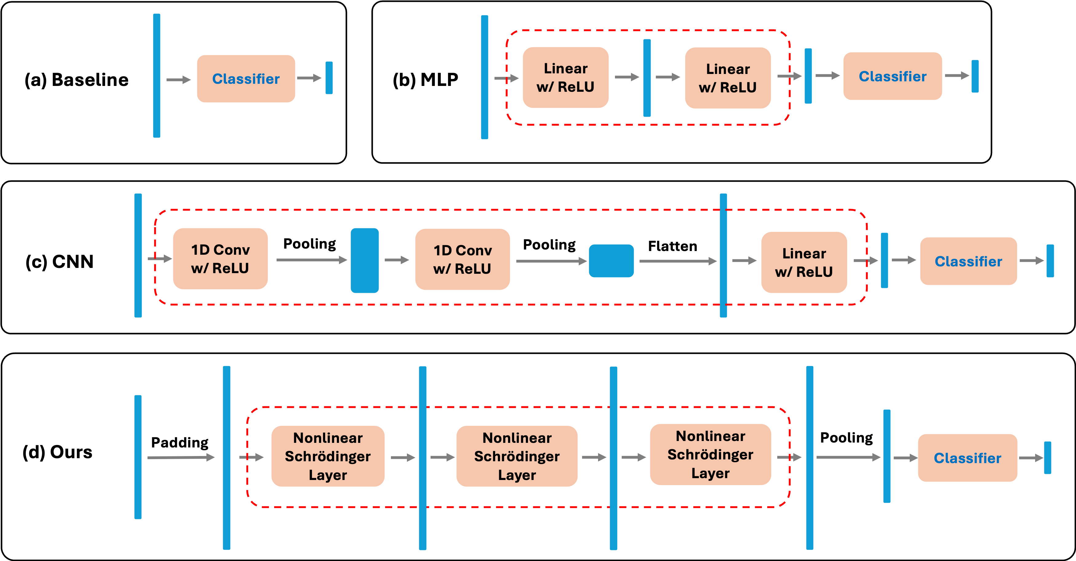
Table 1 presents the accuracy and the number of trainable parameters among four different models across the three datasets. The model architectures are visualized in Figure 2. The baseline is a linear classifier consisting of a single densely connected layer. Multi-Layer Perceptron (MLP) is a feedforward neural network with several densely connected hidden layers and nonlinear activations. The 1D Convolutional Neural Network (CNN) includes a few convolutional layers cascaded with densely connected linear layers. In our proposed Nonlinear Schrödinger Network, we add a max pooling layer after the cascaded Nonlinear Schrödinger Layers to mitigate the dimension increase caused by the zero-padding, and a densely connected linear layer to match the output dimension to the number of classes. All models are trained with the Adam optimizer using the cross-entropy loss. As shown in Figure 2, we divide the model architecture into two parts: the “embedding” layers (red dashed box) that maps the original data into a more linearly separable space, and a linear classifier that makes the final decision on the class to which the transformed data belongs. Note that there is no embedding layer in the baseline model.

| Starlight | Ford Engine | Spoken Digits | ||||
| Metrics | Param # | Acc (%) | Param # | Acc (%) | Param # | Acc (%) |
| Baseline | 3,072 | 84.6 (0.6) | 500 | 49.1 (0.5) | 51,200 | 15.6 (1.1) |
| MLP | 139,264+192 | 85.8 (0.7) | 72,385+64 | 87.7 (0.7) | 663,754+640 | 23.1 (1.6) |
| CNN | 65,715+96 | 92.0 (1.9) | 32,153+32 | 89.5 (1.8) | 327,866+320 | 61.9 (8.4) |
| Ours | 18+3,072 | 92.1 (1.5) | 18+500 | 86.2 (3.3) | 18+51,200 | 70.1 (2.5) |
| \botrule | ||||||
The baseline results obtained using only a linear classifier demonstrate poor performance, particularly on linearly non-separable datasets such as Ford Engine and Spoken Digits. This highlights the inherent limitations of linear classifiers in capturing complex patterns and relationships in the data. In contrast, our proposed Nonlinear Schrödinger Network significantly improves the classification accuracy by incorporating several Nonlinear Schrödinger Layers as embedding layers preceding the linear classifier. Each added layer only introduces 3 extra parameters to the model as discussed earlier, efficiently parameterizing the nonlinear transformation that projects the original data into a more linearly separable space, thereby improving the performance of the same linear classifier used in the baseline model. The results reported here for the Nonlinear Schrödinger Network utilize 6 layers for all three datasets. Therefore, the Nonlinear Schrödinger Network introduces only 18 additional trainable parameters compared to the baseline model as highlighted in the Table. This is a notable advantage of the Nonlinear Schrödinger Network, as it can achieve high performance with a minimal increase in model complexity.
We further compare the Nonlinear Schrödinger Network with conventional neural networks, including Multilayer Perceptrons (MLPs) and 1D Convolutional Neural Networks (CNNs). As shown in Table 1, the Nonlinear Schrödinger Network achieves comparable or better accuracy while maintaining significantly fewer parameters. Notably, the number of trainable parameters in the embedding layers of the Nonlinear Schrödinger Network is orders of magnitude fewer than MLP and CNN, as highlighted in red. These results demonstrate the effectiveness of the proposed Nonlinear Schrödinger Layers in capturing the complex nonlinear dynamics of time series data while maintaining a compact model size. This could be a potential solution to the Memory Wall, which is the gap between the performance of the processor and memory in computer architecture. More importantly, the trained Nonlinear Schrödinger Network is an interpretable model with all the parameters having physical meanings as properties of a virtual physical system. This interpretability is a significant advantage over traditional black-box neural networks, as it allows us to gain deeper insights into the underlying dynamics of the data and the decision-making process of the model.
4.2 Learning Curve and Parameter Convergence


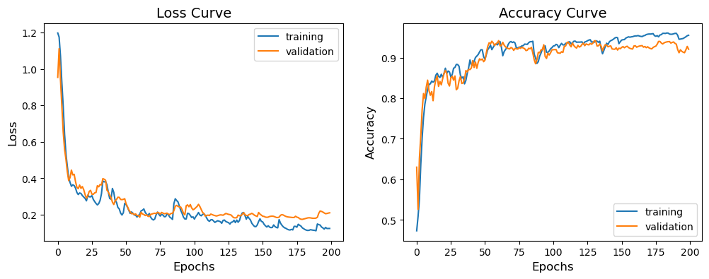
Figure 3 illustrates the learning curves of the Nonlinear Schrödinger Network trained on the Starlight dataset. As the training progresses, the loss decreases steadily while the accuracy improves for both the training and validation datasets. This indicates successful optimization of the network using backpropagation, demonstrating the network’s ability to learn and generalize from the training data.
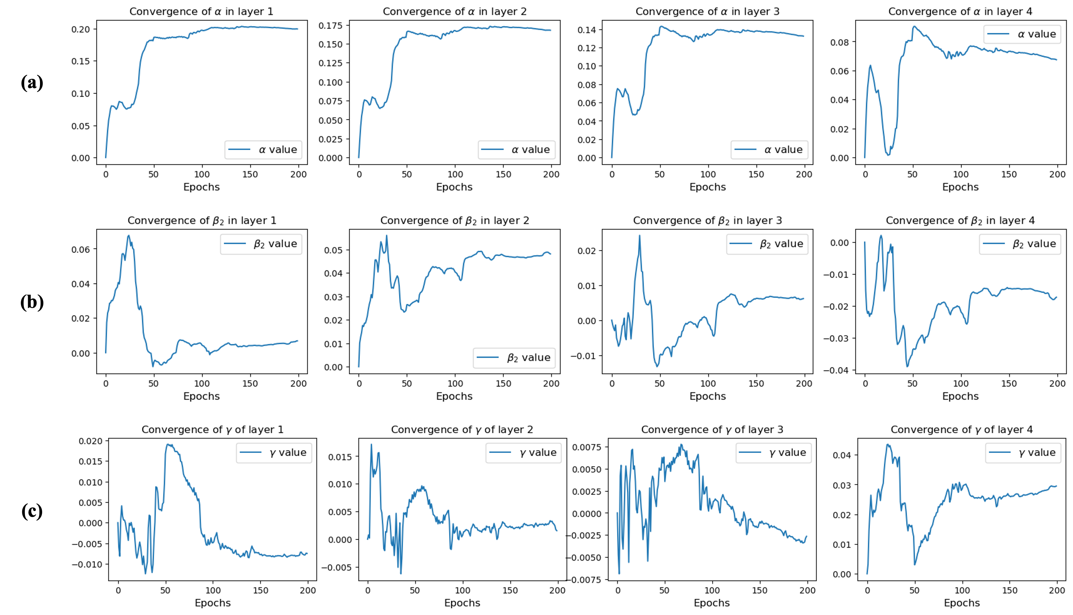
Figure 4 presents the convergence of the key parameters , and in the first four layers of the Nonlinear Schrödinger Network during training on the Starlight dataset. Initially, all parameters are set to zero. As the training progresses, these parameters gradually converge to values that optimize the network’s classification performance. Notably, they can be interpreted as the properties of a virtual physical system that transforms the original data to another space for improved classification accuracy.
4.3 Ablation Study on the Impact of Dispersion and Nonlinearity
In this section, we conduct an ablation study to investigate the effects of the linear operations (), as shown in Equation 2, and the nonlinear operations (), as shown in Equation 3, within the Nonlinear Schrödinger Network. This study aims to provide insights into the network’s underlying mechanisms and how these components interact to achieve improved performance.
To accomplish this, we first train the network using only the linear operations () by setting and updating only and across all layers during the training process. Similarly, we then train the network using only the nonlinear operations () by setting and updating only across all layers during training. The results of these ablated models are compared with the baseline (a linear classifier only) and the full Nonlinear Schrödinger Network (with both linear and nonlinear effects enabled) in Table 2.
| Model | Ford Engine Acc (%) | Spoken Digits Acc (%) |
|---|---|---|
| Baseline | 49.1 (0.5) | 15.6 (1.1) |
| Only | 51.7 (1.2) | 19.9 (1.9) |
| Only | 79.5 (6.2) | 60.3 (5.5) |
| Full | 86.2 (3.3) | 70.1 (2.5) |
| \botrule |
The results demonstrate that the model with only linear operations () achieves significant improvement over the baseline. In contrast, the model with only nonlinear operations () shows barely any improvement over the baseline. The full model, incorporating both linear and nonlinear components, yields the best results overall.
These findings can be attributed to the data processing method employed in the Nonlinear Schrödinger Network. The input data is amplitude modulated onto the real input . After propagation through the network, a complex output is obtained, and its amplitude is subsequently fed to the linear classifier. When only the nonlinear operations () are present, the self-phase modulation does not alter the amplitude, resulting in . Consequently, the nonlinear operations alone do not significantly contribute to the network’s performance. On the other hand, when only linear operations () are present, all transformations are linear, except for the final step of taking the amplitude. This allows the linear operations to capture some underlying patterns in the data, leading to improved performance over the baseline.
The true potential of the Nonlinear Schrödinger Network is realized when both linear and nonlinear components are combined. The nonlinear effect of in layer comes into play when followed by a linear operation in layer as the data remains in the complex domain. This coupled interaction between the nonlinear and linear components enables the network to capture complicated patterns and relationships in the data more effectively, resulting in the best overall performance.
5 Discussion
While the Nonlinear Schrödinger Network demonstrates impressive performance, it is essential to acknowledge that its generalizability might be less than that of traditional DNNs. The model’s design is heavily influenced by the specific physical principles encoded in the NLSE. As a result, it may not be as flexible in handling data that do not conform to the underlying physical assumptions. However, this trade-off between interpretability and generalizability is not necessarily a disadvantage. In many practical applications, a more physically consistent and interpretable model may be preferred, even if it sacrifices some degree of generalizability.
6 Conclusion
In this paper, we have presented the Nonlinear Schrödinger Network, a novel physics-inspired trainable model that leverages the principles of the Nonlinear Schrödinger Equation (NLSE) to learn complex patterns and nonlinear mappings from data. Unlike conventional neural networks, which often rely on large numbers of parameters, our approach directly utilizes the partial differential equation (PDE) that governs physical systems in a trainable and digital form, resulting in an interpretable and parameter-efficient model that can be optimized with backpropagation and gradient descent.
The experiments on various time series classification datasets have demonstrated that the Nonlinear Schrödinger Network achieves comparable or superior accuracy with orders of magnitude fewer parameters than conventional models such as Multi-Layer Perceptrons (MLPs) and Convolutional Neural Networks (CNNs). This highlights the efficiency of our approach in capturing complex dynamics with minimal model complexity. Furthermore, the transformations learned by the Nonlinear Schrödinger Network can be explicitly formulated and interpreted through the lens of a partial differential equation, with each parameter having a clear physical meaning. This contrasts sharply with the black-box nature of typical neural networks, offering insights into the data transformation process and making the model more transparent and understandable. While the current implementation uses the NLSE, the proposed method of using a physics equation as a trainable model to learn nonlinear mappings from data is not restricted to the NLSE but maybe implemented with other equations.
References
- \bibcommenthead
- Karniadakis et al. [2021] Karniadakis, G.E., Kevrekidis, I.G., Lu, L., Perdikaris, P., Wang, S., Yang, L.: Physics-informed machine learning. Nature Reviews Physics 3(6), 422–440 (2021)
- Jalali et al. [2022] Jalali, B., Zhou, Y., Kadambi, A., Roychowdhury, V.: Physics-ai symbiosis. Machine Learning: Science and Technology 3(4), 041001 (2022)
- Raissi et al. [2019] Raissi, M., Perdikaris, P., Karniadakis, G.E.: Physics-informed neural networks: A deep learning framework for solving forward and inverse problems involving nonlinear partial differential equations. Journal of Computational physics 378, 686–707 (2019)
- Li et al. [2020] Li, Z., Kovachki, N., Azizzadenesheli, K., Liu, B., Bhattacharya, K., Stuart, A., Anandkumar, A.: Fourier neural operator for parametric partial differential equations. arXiv preprint arXiv:2010.08895 (2020)
- Lin et al. [2018] Lin, X., Rivenson, Y., Yardimci, N.T., Veli, M., Luo, Y., Jarrahi, M., Ozcan, A.: All-optical machine learning using diffractive deep neural networks. Science 361(6406), 1004–1008 (2018)
- Mohammadi Estakhri et al. [2019] Mohammadi Estakhri, N., Edwards, B., Engheta, N.: Inverse-designed metastructures that solve equations. Science 363(6433), 1333–1338 (2019)
- Zhou et al. [2022] Zhou, T., Scalzo, F., Jalali, B.: Nonlinear schrödinger kernel for hardware acceleration of machine learning. Journal of Lightwave Technology 40(5), 1308–1319 (2022)
- Zhou and Jalali [2023] Zhou, T., Jalali, B.: Low latency computing for time stretch instruments. Journal of Physics: Photonics 5(4), 045004 (2023)
- Liu et al. [2018] Liu, Z., Zhu, D., Rodrigues, S.P., Lee, K.-T., Cai, W.: Generative model for the inverse design of metasurfaces. Nano letters 18(10), 6570–6576 (2018)
- Lim and Psaltis [2022] Lim, J., Psaltis, D.: Maxwellnet: Physics-driven deep neural network training based on maxwell’s equations. Apl Photonics 7(1) (2022)
- Kutz [2017] Kutz, J.N.: Deep learning in fluid dynamics. Journal of Fluid Mechanics 814, 1–4 (2017)
- Agrawal [2000] Agrawal, G.P.: Nonlinear fiber optics. In: Nonlinear Science at the Dawn of the 21st Century, pp. 195–211. Springer, ??? (2000)
- Dau et al. [2019] Dau, H.A., Bagnall, A., Kamgar, K., Yeh, C.-C.M., Zhu, Y., Gharghabi, S., Ratanamahatana, C.A., Keogh, E.: The ucr time series archive. IEEE/CAA Journal of Automatica Sinica 6(6), 1293–1305 (2019)
- Rebbapragada et al. [2009] Rebbapragada, U., Protopapas, P., Brodley, C.E., Alcock, C.: Finding anomalous periodic time series: An application to catalogs of periodic variable stars. Machine learning 74, 281–313 (2009)
- Jackson et al. [2018] Jackson, Z., Souza, C., Flaks, J., Pan, Y., Nicolas, H., Thite, A.: Jakobovski/free-spoken-digit-dataset: v1. 0.8. Zenodo, August (2018)