Catastrophic Goodhart: regularizing RLHF with KL divergence does not mitigate heavy-tailed reward misspecification

Abstract

When applying reinforcement learning from human feedback (RLHF), the reward is learned from data and, therefore, always has some error. It is common to mitigate this by regularizing the policy with KL divergence from a base model, with the hope that balancing reward with regularization will achieve desirable outcomes despite this reward misspecification. We show that when the reward function has light-tailed error, optimal policies under less restrictive KL penalties achieve arbitrarily high utility. However, if error is heavy-tailed, some policies obtain arbitrarily high reward despite achieving no more utility than the base model—a phenomenon we call catastrophic Goodhart. We adapt a discrete optimization method to measure the tails of reward models, finding that they are consistent with light-tailed error. However, the pervasiveness of heavy-tailed distributions in many real-world applications indicates that future sources of RL reward could have heavy-tailed error, increasing the likelihood of reward hacking even with KL regularization.

1 Introduction

Kullback-Leibler (KL) divergence constraints in reinforcement learning (RL) are employed to stay in regimes where the objective is accurate enough. Some on-policy (Schulman et al., 2015, 2017) and many off-policy (Abdolmaleki et al., 2018; Jaques et al., 2019) policy gradient algorithms employ KL constraints or penalties during optimization to prevent the policy from deviating too much from the data collection distribution. This ensures that estimates of each action’s advantage are reliable enough to update the policy in a helpful way.

Reinforcement learning from human feedback (Christiano et al., 2017; Ziegler et al., 2020, RLHF) is a very popular method to induce desirable behavior in language models. RLHF starts with a base pre-trained model, then learns a reward function from human annotator data. Next, it trains an RL policy to maximize this reward, while penalizing high KL divergence from the policy to the base model. RLHF uses an on-policy algorithm and has accurate advantages, but the reward function is always somewhat misspecified compared to desired behavior, due to insufficient data, human biases, and other factors.

The main purpose of the KL penalty in RLHF is to limit the consequence of reward modeling errors by keeping the policy within a distribution similar to that on which it was trained. Ideally, in the low-KL regime the reward model’s errors are small enough that it provides correct updates to the base model. Gao et al. (2023) empirically supports this view: if the KL divergence in RLHF is allowed to grow too much, with a misspecified reward, the model’s performance on the true utility starts to decrease.

We ask: can we obtain good outcomes from misspecified reward in RLHF by controlling the KL divergence? That is, if there is some error between the true reward $V$ and the proxy reward $U$, can the KL help us to still optimize $V$? Using mathematical proof, we answer the question in the negative for heavy-tailed errors: there exist policies which have infinite proxy reward $U$, but whose KL with the base model vanishes (these have undetermined $V$). We term this phenomenon “catastrophic Goodhart”, after Goodhart’s law.

If the misspecification errors are independent and light-tailed, the KL divergence does suffice to guarantee good outcomes. There may also be guarantees under weaker assumptions, but assumptions that intuitively seem sufficient are often not (see Section 6).

Possibly, other regularization schemes would guarantee good outcomes for heavy-tailed errors, but this is not just a problem of KL. We show that optimizing by conditioning on large reward $U$ has similar outcomes in light- and heavy-tailed regimes.

Empirically, open-source language reward models seem to be light-tailed, which does not imply light-tailed errors but suggests it (Section 5). However, the errors are likely not independent and, given the prevalence of heavy-tailed distributions in the real world, error in future reward models may also be heavy-tailed. In any case, the present success of RLHF with misspecified rewards cannot be explained solely by the KL regularization in its objective.

2 Background

2.1 KL divergence and KL regularization

Recall that KL divergence between two distributions P and Q is defined as $D_{\mathrm{KL}}(P\|Q)=\sum_{x\in\mathcal{X}}P(x)\log\left(\frac{P(x)}{Q(x)}\right)$.

If we have two policies $\pi,\pi_{0}$, we define $D_{KL}(\pi\|\pi_{0})$ as the KL divergence between the distributions of actions taken on the states in trajectories reached by $\pi$. That is, if $Tr(\pi)$ is the distribution of trajectories taken by $\pi$, we penalize $D_{KL}(\pi\|\pi_{0})\triangleq\mathbb{E}_{s\in T,T\sim Tr(\pi)}[D_{KL}(\pi(s)\|\pi_{0}(s))]$.

In RLHF, it is common to use the regularization term $\beta D_{KL}\left(\pi\|\pi_{0}\right)$ to prevent the learned policy from deviating too much from the base policy, which can prevent unstable behavior or overfitting to the reward model. If our reward model gives reward $U$, then the optimal policy for RLHF with a KL penalty is $\arg\max_{\pi}\mathbb{E}[U(\pi)]-\beta D_{KL}\left(\pi\|\pi_{0}\right).$

Often the regularization parameter $\beta$ is dynamically adjusted to keep the $D_{KL}$ near some target value (Ziegler et al., 2020).

2.2 Heavy-tailed distributions

A distribution $P$ over $\mathbb{R}$ with cumulative distribution function (CDF) $F_{P}$ is heavy-tailed if its tail function $\bar{F}_{P}(x)\triangleq 1-F_{P}(x)$ satisfies $\lim_{x\rightarrow\infty}e^{tx}\bar{F}(x)=\infty$ for all $t>0$. Heavy-tailed distributions are well-known in statistics to have a higher probability of producing a single extreme value. For example, if the sum of two independent variables from heavy-tailed distributions is large, it is most likely due to one extreme sample rather than two equally large samples. (Wierman, 2013)

2.3 Reward misspecification and Goodhart’s Law

Reward misspecification has caused low-utility outcomes in practice; for example, in (Clark & Amodei, 2016), an RL agent trained to play a racing videogame according to a misspecified reward function achieves a high score while failing to complete the course.

Gao et al. (2023) introduce the concept of “overoptimization”: optimizing for a proxy objective decreases performance according to the true objective. This raises the question: in general, when RLHF reward is misspecified, when does the optimal policy produce high utility?

By applying the proxy reward and true reward functions to a distribution over text (generated by an LLM), we get two scalar random variables, which we call $U$ for proxy reward and $V$ for true reward / utility. Then we can define the error in the proxy reward as $X\triangleq U-V$, so that $U=X+V$. Framed this way, optimization for a proxy reward $U$ is a mix of desirable optimization for $V$ and undesirable optimization for $X$. The joint distribution of $V$ and $X$ determines the limiting value of $V$ as we apply more optimization. When we say that reward misspecification can have negative effects, we mean that too much variance in $X$ can "redirect" the optimization pressure from $V$ to $X$, and prevent utility gain from optimization.

Reward misspecification is also studied by (Lambert & Calandra, 2024), (Laidlaw et al., 2024), and others. Laidlaw et al show that a KL penalty between action distributions can be ineffective, and propose instead regularizing state occupancy measure. Our results show an inherent weakness of KL divergence, including when applied to state occupancy measure.

3 Theoretical results

When applying KL regularization, the trained model is regularized towards some base policy $\pi_{0}$. One would hope that a KL penalty can produce good outcomes even in the case of reward misspecification; that is, if the reward $U$ is the sum of true utility $V$ and an error term $X$, we would hope that optimal policies under a KL penalty achieve high $V$ even if the magnitude of $X$ is large. We show that this is not always the case: Corollary 1 of Theorems 1, 2, and 3 establishes that when $X(\pi_{0})$ is heavy-tailed, there are arbitrarily well-performing policies $\pi$ with $\mathbb{E}_{\pi}[V]\approx\mathbb{E}_{\pi_{0}}[V]$. However, Theorem 4 shows that when error is light-tailed and independent of $V$, the optimal policy under a KL penalty results in $V>0$, and $V$ can be made arbitrarily large. Thus, the tails of the error distribution are crucial in determining how much utility will result from optimization towards an imperfect proxy.

Theorems 5 and 8 (Section B of the appendix) show that the relationship of catastrophic Goodhart to heavy-tailed error is not just a quirk of KL divergence by using a different model of optimization based on conditioning on high reward values. Under this model (and given additional regularity conditions), it is also true that heavy-tailed error results in catastrophic Goodhart, and light-tailed error plus independence results in arbitrarily large utility. All proofs are in the appendix.

3.1 Heavy-tailed distributions

Theorem 1.

Given any heavy-tailed reference distribution $Q$ over $\mathbb{R}$ with mean $\mu_{Q}$, and any $M,\epsilon>0$, there is a distribution $P$ with mean $\mu_{P}>M$ and $D_{KL}(P\|Q)<\epsilon$.

Outline of proof (see appendix for full proof): WLOG take $\mu_{Q}=0$. If we set $P_{t}$ to upweight the probability mass of $Pr_{P_{t}}(X>t)$ to $c/t$ for some $c,t$, then the mean of $P_{t}$ will be approximately at least $c$. As $t\to\infty$, the KL divergence $D_{KL}(P_{t}\|Q)$ will shrink to zero.

3.2 RLHF with KL penalty under heavy-tailed return distribution

We now adapt our result to the case where the policy is a language model and we are training it using RLHF. We are now applying KL divergence over the policies rather than the return distributions. We first formally define the properties of RLHF on language models that cause the result to hold: namely, when when considered as a Markov decision process (MDP), environmental transitions are deterministic and return depends only on the final state reached.

Definition: A deterministic-transition MDP with Markovian returns (DMRMDP) is an MDP $(\mathcal{S},\mathcal{A},P,R)$ such that:

• The transition function $P:\mathcal{S}\times\mathcal{A}\to\mathcal{S}$ is deterministic, i.e., for each state $s\in\mathcal{S}$ and action $a\in\mathcal{A}$, there exists a unique state $s^{\prime}\in\mathcal{S}$ such that $P(s^{\prime}|s,a)=1$.
  In RLHF: the transition is appending the generated token $a$ to the context $s$.

• There is a set of sink states $E\subseteq\mathcal{S}$ that terminate a trajectory, which is disjoint from the set of start states.
  In RLHF: The sink states are sequences ending in <EOS> or above a certain length.

• Returns are Markovian; that is, for any two trajectories $\tau=(s_{1},a_{1},\dots,s_{n}),\tau^{\prime}=(s_{1}^{\prime},a_{1}^{\prime},\dots,s_{n}^{\prime}),$ if $s_{n}=s^{\prime}_{n}$, then $\tau$ and $\tau^{\prime}$ have identical return distributions. Equivalently, for the trajectory random variable $T=(S_{1},A_{1},\dots)$ distributed according to any policy, with return $G$, $G\bot\!\!\!\!\!\ \bot(S_{<i},A_{<i})\ |\ S_{i}$ for any $i\geq 1$.
  In RLHF: the return only depends on the full generated string, which is the final state.

The language model stochastically outputs the next token $a$ given $s$, and corresponds to the policy. A DMRMDP is therefore a good model of RLHF.

Theorem 2.

Let $W=(\mathcal{S},\mathcal{A},P,R)$ be a deterministic-transition MDP with Markovian returns. Given $W$ we define the function that takes policies to trajectories $Tr:(S\to\Delta A)\to\Delta(S\times A)^{*}$, and the average return function $g:(S\times A)^{*}\to\mathbb{R}$, which induces a function $G:\Delta(S\times A)^{*}\to\Delta\mathbb{R}$. Let $\pi_{0}:\mathcal{S}\to\Delta\mathcal{A}$ be some base policy. If $G\circ Tr(\pi_{0})$ is heavy-tailed with finite mean $\mu_{Q}$, then for any $M,\epsilon>0$, there is a policy $\pi$ with mean return $\mathbb{E}[U|U\sim G\circ Tr(\pi)]>M$ and $\mathbb{E}_{s\in T,T\sim Tr(\pi)}[D_{KL}(\pi(s)\|\pi_{0}(s))]<\epsilon$.

3.3 If V is light-tailed, $\mathbb{E}_{P}[V]\!-\!E_{Q}[V]\to 0$ as $D_{KL}\!\to\!0$

Theorem 3.

If $V$ is light-tailed and $d=D_{KL}(P\|Q)$ is bounded, then $\mathbb{E}_{P}[V]$ is bounded, and $\mathbb{E}_{P}[V]-\mathbb{E}_{Q}[V]\to 0$ as $d\to 0$.

Corollary 1.

Theorems 2 and 3 imply that when utility is light-tailed, reward modeling errors make the proxy reward heavy-tailed, and a policy $\pi$ is regularized severely enough to have KL divergence values approaching zero, the reward $\mathbb{E}[U(\pi)]$ can go to infinity while utility $\mathbb{E}[V(\pi)]$ approaches a value no higher than the base policy.

3.4 Light-tailed + independence imply $\mathbb{E}[V]\to\infty$

Theorem 4.

If $U=X+V$ with $X$ and $V$ both light-tailed, and the distribution of U is continuous, and $\pi^{*}(\beta)\triangleq\arg\max_{\pi}\mathbb{E}[U(\pi)]-\beta D_{KL}(\pi,\pi_{0})$, then $\lim_{\beta\to 0^{+}}\mathbb{E}[V(\pi^{*}(\beta))]=\infty$.

4 Experimental Methodology

Our theoretical results now raise the question of whether the error in reward models is heavy-tailed or light-tailed in practice. If we observe the reward distribution to be light-tailed, this is a strong indication that error is light-tailed.

To empirically test whether the reward is heavy-tailed, we consider two lines of evidence: examining the distributions directly through random sampling and temperature-1 sampling, and finding adversarial token sequences that get high rewards. We examine one small and one medium reward model that performed reasonably well on RewardBench (Lambert et al., 2023). The small model is an OpenAssistant model based on Pythia 1.4B, and the medium model is Starling 7B-alpha (Zhu et al., 2023).

For random sampling, we sample 30000 length-1024 sequences of uniformly random tokens and observe the distribution of rewards assigned by both Pythia 1.4B and Llama 7B-chat. We also use Llama 7B-chat to generate 16000 length-133 sequences and observe the distribution of rewards assigned by Starling 7B-alpha.

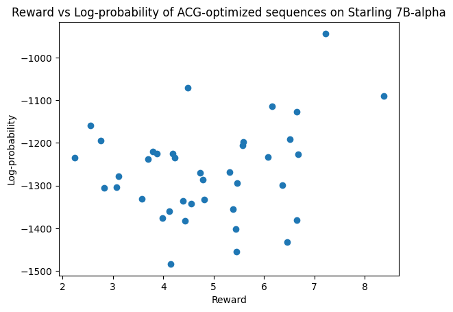
Because sampling is inefficient at probing the extreme tail, we also find token sequences that optimize Starling 7B-alpha for reward. We considered Greedy Coordinate Gradient (GCG) from (Zou et al., 2023), a method used to find adversarial suffixes that circumvent jailbreaking, but decided on a faster version of GCG called Accelerated Coordinate Gradient (ACG) from (Haize Labs, 2024). See Table 1 for ACG hyperparameters.

Generating plots took about 5 GPU-hours on 1x Nvidia H100, and running ACG took a further 8 hours.

5 Results

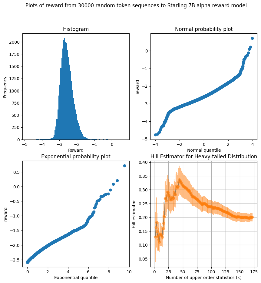
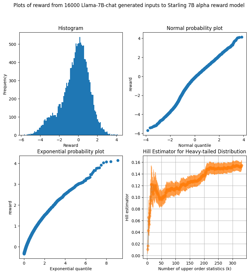
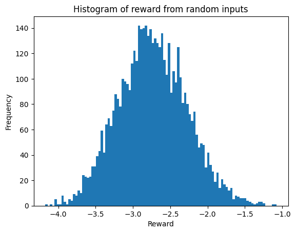
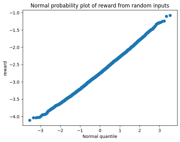
When sampling token sequences, both the Pythia model on random inputs (Figure 5) and Starling 7B-alpha on Llama-generated inputs (Figure 2) appear approximately normal and, therefore, light-tailed. Starling on random inputs (Figure 1 is ambiguous, with the exponential Q-Q plot having an outlier that could indicate a heavy-tailed distribution, but the Hill estimator is consistent with a light-tailed distribution. Because Llama-7B-chat is a more reasonable base model than a completely random policy, we believe that Starling 7B-alpha is more likely to be light-tailed for the purposes of our theoretical results.

Figure 1: Plots of the distribution of reward from 30000 random length-1024 token sequences to Starling 7B-alpha. Clockwise from top left: The histogram shows a unimodal distribution with a slight right skew. The normal probability plot indicates the data are heavier-tailed than normal. The Hill estimator (error bars are standard error) appears to be 0.20 for higher values but fluctuates for lower values. The exponential probability plot of the right half of the distribution is consistent with either light or heavy tails (under heavy tails, the slope would go to infinity).

Figure 2: Plots of the reward distribution from 16000 token sequences generated by Llama 7B-chat of length $\leq 133$, starting with five random tokens. Clockwise from top left: A histogram shows the reward distribution has a left skew. The normal probability plot suggests reward is approximately normal and thus light-tailed. The Hill estimator plot should stabilize if the distribution is heavy-tailed, but it does not; thus, there is no evidence the distribution is heavy-tailed. The exponential probability plot also indicates light tails, because the curve is bending downwards.

The ACG results need some interpretation. The KL divergence between two distributions $P$ and $Q$ if $P$ is the same as $Q$ a fraction $1-\alpha$ of the time, but is some value $x$ a fraction $\alpha$ of the time is given by $D_{KL}(P\|Q)=\left[(1-\alpha)q(x)+\alpha\right]\log\left(\frac{(1-\alpha)q(x)+\alpha}{q(x)}\right)+(1-\alpha)\log(1-\alpha)(1-q(x))$.

When $\alpha$ is small but much larger than $q(x)$, we approximate this to first order as $D_{KL}(P\|Q)\approx\alpha\log\left(\frac{\alpha}{q(x)}\right)$. In Theorems 1 and 2, we prove that when the error is sufficiently heavy-tailed, a policy that gets extremely large reward a small fraction of the time will achieve high expected reward with low KL divergence. This is not the case here because the rewards achieved through ACG were small and the log-probabilities extremely negative. For example, a policy that matches Llama 2-chat’s base reward 99% of the time and uses the highest-reward input generated by ACG $\alpha=$1% of the time will have KL divergence from Llama 2-chat of $\alpha(\log(\alpha)-1339.70)=13.35$ nats, but reward only about $\alpha*(2.2377-0.3329)=0.02571$ greater than the base model, far less than can be obtained with the same KL divergence by conditioning.

6 Discussion and Limitations

6.1 How likely is catastrophic Goodhart?

The low-KL policies that result in catastrophic Goodhart are not a unique optimal policy, just one family of high-performing policies. When optimizing $\mathbb{E}[U(\pi)]-\beta D_{KL}\left(\pi,\pi_{0}\right)$, the outcome depends on RL training dynamics; it could be that $D_{KL}\to 0$ causing catastrophic Goodhart, but more likely both terms will go to infinity, potentially allowing $V\to\infty$. Catastrophic Goodhart can be prevented by using a light-tailed or bounded reward function.

Even so, catastrophic Goodhart is likely to occur in many scenarios where KL regularization is naively employed in an attempt to avoid Goodhart’s Law:

• If we maximize $\sigma(\mathbb{E}[U])+D_{KL}(Tr(\pi)\|Tr(\pi_{0}))$, where $\sigma$ is a bounded function (e.g. sigmoid), all near-optimal policies will have $V\approx 0$. Since we can only obtain so much reward from $\sigma(\mathbb{E}[U])$, it pays to make the KL (and thus V) go to zero.

• If we cap KL to a finite value (or dynamically adjust the KL penalty to target a finite KL, as done in Ziegler et al. (2020), then $\mathbb{E}[V]$ is also upper bounded by a finite value (see Theorem 3), and we think it is likely that $\mathbb{E}[V]\approx 0$. Consider a toy model where an AI can adjust three parameters: true quality $V$ of responses, frequency of reward hacking (producing actions with extremely high X), and severity of hacking (value of X on those actions). Adjusting the policy to increase $\mathbb{E}[U]$ without increasing KL increase the severity of hacking while decreasing either frequency of hacking or quality of responses. When $E[U]$ is already large, decreasing quality has much better returns than decreasing frequency. This is similar to Theorems 5, 8 about hard-threshold optimization.

• Any way we maximize $\mathbb{E}[U(\pi)]-\beta D_{KL}\left(\pi,\pi_{0}\right)$ results in very large values of $\mathbb{E}[U(\pi)]$, and there are a number of arguments that extreme optimization for an imperfect proxy can result in decreased utility due to tradeoffs between $X$ and $V$; e.g., the constrained resource scenario in (Zhuang & Hadfield-Menell, 2021).

6.2 Independence assumptions

Theorems 2 and 3 do not require any independence assumption, but Theorems 4, 5, and 6 require that error $X$ and utility $V$ are independent, which seems to be violated in practice. Future work could weaken this assumption, although intuitively obvious ways to weaken it result in the statement being false.

6.3 Stronger optimization methods

We did not search the entire space of token sequences, so we cannot rule out that the reward is heavy-tailed enough to cause catastrophic Goodhart in some situations. While it is intractable to search the more than $10^{2000}$ possible token sequences, future work could get more evidence through more powerful optimization methods.

6.4 Relation to previous overoptimization work

Gao et al. (2023) found that optimizing the reward of small reward models causes overoptimization: a decrease in utility with increasing optimization. However, we observed that reward models are light-tailed, and (Theorem 4) that independence combined with light-tailed error prevents overoptimization. We think this discrepancy is explained by dependence between error and utility. Policies optimized for high error may activate features in the proxy reward models that are undesirable according to the true utility function. More research is needed to understand why high-error completions have low utility and to design reward models that do not suffer from this problem; Perhaps it is possible to construct reward models whose errors are in directions orthogonal to human preferences, so that the large-reward completions do not have lower utility.

7 Conclusion

We have argued that the purpose of the KL divergence regularization in RLHF is to mitigate reward misspecification. However, we have also proven that when errors in the reward function are heavy-tailed, it cannot serve this purpose: even with zero KL divergence, there are policies that achieve very high misspecified reward and no actual reward.

When errors are light-tailed and independent, the KL divergence can mitigate misspecification, but when they are dependent, this may not be possible. Thus, we must look to places other than the KL objective to explain the current success of RLHF and ensure its continued success in the future.

Impact Statement

As this work aims to improve the safety of future ML systems by characterizing a possible failure mode of reward misspecification in RLHF, we hope the social impact is positive. We see no particular ethical issues to discuss.

Appendix A Proofs

A.1 Theorem 1

Restatement of Theorem 1.

Given any heavy-tailed reference distribution $Q$ over $\mathbb{R}$ with mean $\mu_{Q}$, and any $M,\epsilon>0$, there is a distribution $P$ with mean $\mu_{P}>M$ and $D_{KL}(P\|Q)<\epsilon$.

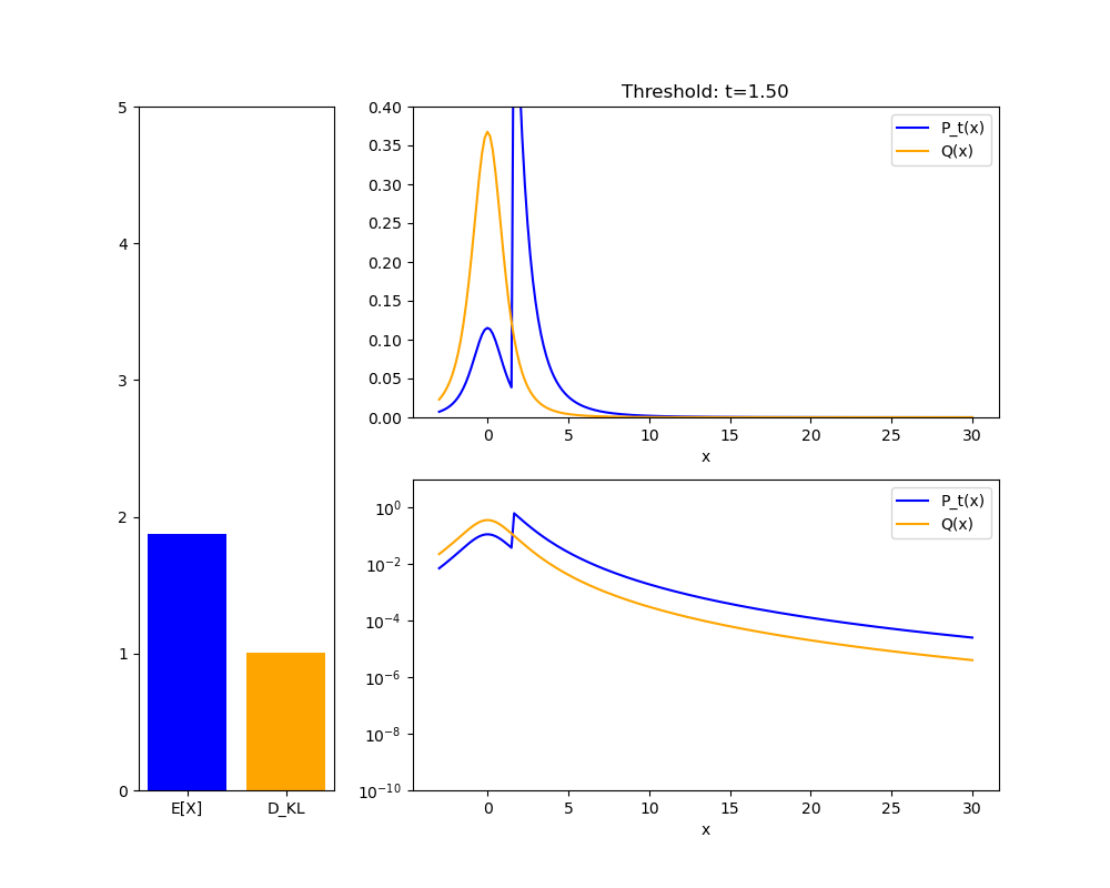
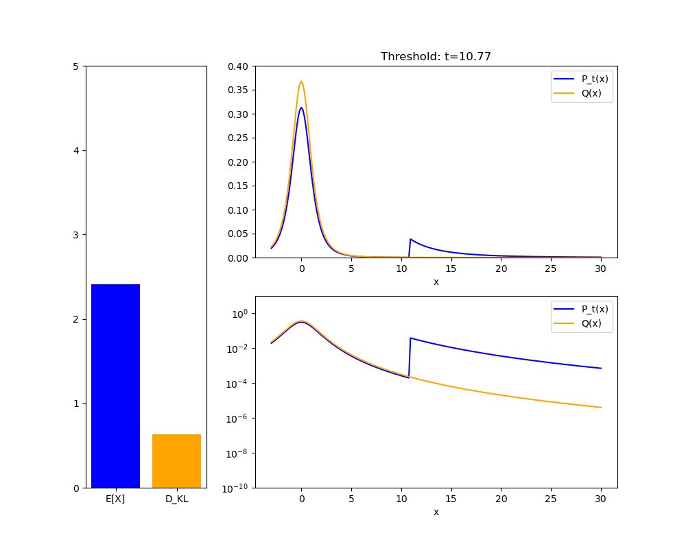
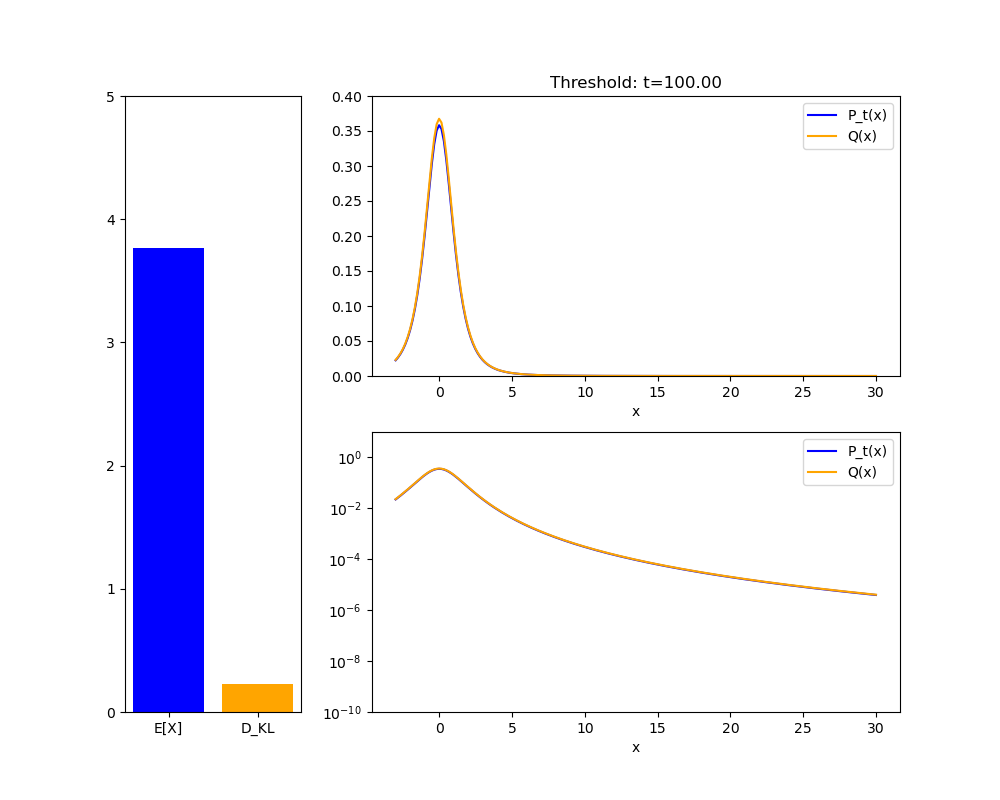
Intuitively, in a heavy-tailed distribution, events with extremely high $x$ are not very rare, so you don’t pay much of a KL penalty to upweight them so they happen about $1/x$ of the time. This is visually illustrated in Figure 3.

Figure 3: As $t\to\infty$, the mean of $X$ (blue bar) grows without bound while KL divergence $D_{KL}(P_{t}\,\|\,Q)$ (orange bar) goes to 0. The base distribution Q is a Student t-distribution with $df=3$. In this case, high values of X are upweighted to $1/t^{0.8}$; upweighting them to $1/t$ would cause $\mathbb{E}[X]$ to converge to  $1$ while KL divergence goes to zero faster.

Proof. WLOG let $\mu_{Q}=0$. We construct a sequence of distributions $\{P_{t}\}$ such that $\lim_{t\to\infty}\mathbb{E}_{P_{t}}[X]\geq c$ for any constant $c$, and $\lim_{t\to\infty}D_{KL}(P_{t}\|Q)=0$. We define $P_{t}$ for any $t>c$ thusly. Writing $F_{P_{t}}(x)$ for the CDF $Pr_{X\sim P_{t}}(X\leq x)$ and $\bar{F}_{P_{t}}(x)$ for $1-F_{P_{t}}(x)$, we let

$$\bar{F}\_\{P\_t\}(x)=\begin{cases}1-\frac{1-c/t}{F_{Q}(t)}F_{Q}(x)&x\leq t\\ \frac{c/t}{\bar{F}_{Q}(t)}\bar{F}_{Q}(x)&x>t\end{cases}$$

Intuitively, we rescale the part of the distribution to the right of $t$ evenly to have total probability $c/t$, which is less than 1 because $t>c$.

We must check that $\lim_{t\to\infty}\mathbb{E}_{P_{t}}[X]=c$. We can write

$$\mathbb{E}_{P_{t}}[X]=F_{P_{t}}(t)\mathbb{E}_{P_{t}}[X|X\leq t] +\bar{F}_{P_{t}}(t)\mathbb{E}_{P_{t}}[X|X>t]$$

$$=F_{P_{t}}(t)\mathbb{E}_{Q}[X|X\leq t] +\bar{F}_{P_{t}}(t)\mathbb{E}_{Q}[X|X>t]$$

$$=F_{Q}(t)\mathbb{E}_{Q}[X|X\leq t] +\bar{F}_{Q}(t)\mathbb{E}_{Q}[X|X>t]+$$

$$(F_{P_{t}}(t)-F_{Q}(t)) E_{Q}[X|X\leq t]+(\bar{F}_{P_{t}}(t)-\bar{F}_{Q}(t))E_{Q}[X|X>t]$$

$$=\mathbb{E}_{Q}[X]+(\bar{F}_{P_{t}}(t)- \bar{F}_{Q}(t))(E_{Q}[X|X>t]-E_{Q}[X|X\leq t])$$

We know that $\mathbb{E}_{Q}[X|X>t]>t$ because it is an integral of values strictly greater than t. Because $\mathbb{E}_{Q}[X]=0$ is a weighted average of $\mathbb{E}_{Q}[X|X>t]$ and $E_{Q}[X|X\leq t]$, and $\mathbb{E}_{Q}[X|X>t]>0$, we know $E_{Q}[X|X\leq t]<0$. So $E_{Q}[X|X>t]-E_{Q}[X|X\leq t]>t.$ We also know that for sufficiently large $t$, $(F_{P_{t}}(t)-F_{Q}(t))>0$. Intuitively, starting from $Q$, which has mean 0, $P_{t}$ moves a probability mass approaching $\frac{c}{t}$ from mean <0 to mean >t.

Now we can say

$$\lim_{t\to\infty}\mathbb{E}_{P_{t}}[X]>\lim_{t\to\infty}\left[\mathbb{E}_{Q}[X]+(\bar{F}_{P_{t}}(t)-\bar{F}_{Q}(t))(t-0)\right]\\ =\lim_{t\to\infty}\left(\frac{c}{t}-\bar{F}_{Q}(t)\right)t=\lim_{t\to\infty}c-t\bar{F}_{Q}(t)$$

Because $Q$ has a finite mean, $\lim_{t\to\infty}t\bar{F}_{Q}(t)=0$, and so $\mathbb{\lim}_{t\to\infty}\mathbb{E}_{P_{t}}[X]\geq c$.

Now we check that $\lim_{t\to\infty}D_{KL}(P_{t}\|Q)=0$:

$$D_{KL}({P_{t}}\|Q) =\int_{\mathbb{R}}\log\frac{{P_{t}}(dx)}{Q(dx)}\,{P_{t}}(dx)$$

$$=\int_{x\leq t}\log\frac{{P_{t}}(dx)}{Q(dx)}\,{P_{t}}(dx)+\int_{x>t}\log\frac{{P_{t}}(dx)}{Q(dx)}\,{P_{t}}(dx)$$

$$=F_{P_{t}}(t)\log\frac{F_{P_{t}}(t)}{F_{Q}(t)}+\bar{F}_{P_{t}}(t)\log\frac{\bar{F}_{P_{t}}(t)}{\bar{F}_{Q}(t)}\text{\quad since both ratios are constant}$$

$$=F_{P_{t}}(t)\log\frac{1-c/t}{F_{Q}(t)}+\bar{F}_{P_{t}}(t)\log\frac{\bar{F}_{P_{t}}(t)}{\bar{F}_{Q}(t)}$$

Since both $1-c/t$ and $F_{Q}(t)$ go to $1$ as $t\to\infty$, the left term goes to $0$, and so

$$\lim_{t\to\infty}D_{KL}(P_{t}\|Q) \leq 0+\lim_{t\to\infty}\bar{F}_{P_{t}}(t)\log\frac{\bar{F}_{P_{t}}(t)}{\bar{F}_{Q}(t)}$$

$$=\lim_{t\to\infty}\frac{c}{t}\log\frac{c}{t\bar{F}_{Q}(t)}\leq\lim_{t\to\infty}\frac{c}{t}\log\frac{1}{\bar{F}_{Q}(t)}$$

$$=\lim_{t\to\infty}-\frac{c}{t}\log\bar{F}_{Q}(t)\text{\quad since t>c}$$

$Q$ is heavy-tailed, so by definition $\lim_{t\rightarrow\infty}e^{at}\bar{F}_{Q}(t)=\infty\quad\text{ for all }a>0$. This implies that for every $a>0$ there is a sufficiently large $t_{c}$ so that for all $t>t_{c}$, $\bar{F}_{Q}(x)>e^{-at}$, which means that $\log\bar{F}_{Q}(t)>-at$.

Therefore for every $a>0$, $\lim_{t\to\infty}D_{KL}(P_{t}\|Q)\leq\lim_{t\to\infty}-c/t\log\bar{F}_{Q}(t)<\lim_{t\to\infty}-\frac{-act}{t}=ac$, which since KL divergence is nonnegative means that$\lim_{t\to\infty}D_{KL}(P_{t}\|Q)=0$ as desired. $\blacksquare$

A.2 Theorem 2

Restatement of Theorem 2.

Let $W=(\mathcal{S},\mathcal{A},P,R)$ be a deterministic-transition MDP with Markovian returns. Given $W$, we define the function that takes policies to trajectories $Tr:(S\to\Delta A)\to\Delta(S\times A)^{*}$, and the average return function $g:(S\times A)^{*}\to\mathbb{R}$ which induces a function $G:\Delta(S\times A)^{*}\to\Delta\mathbb{R}$. Let $\pi_{0}:\mathcal{S}\to\Delta\mathcal{A}$ be some base policy. If $G\circ Tr(\pi_{0})$ is heavy-tailed with finite mean $\mu_{Q}$, then for any $M,\epsilon>0$, there is a policy $\pi$ with mean return $\mathbb{E}[U|U\sim G\circ Tr(\pi)]>M$ and $\mathbb{E}_{s\in T,T\sim Tr(\pi)}[D_{KL}(\pi(s)\|\pi_{0}(s))]<\epsilon$.

Proof: We will exhibit a distribution of trajectories $\rho$ such that $D_{KL}(\rho\|Tr(\pi_{0}))<\epsilon$ and $\mathbb{E}[G(\rho)]>M$, and then construct a policy $\pi$ with $Tr(\pi)=\rho$. Note that this proof applies for continuous action spaces if trajectories are replaced with measurable sets, but this would make it harder to read.

Let $\rho_{\pi_{0}}=Tr(\pi_{0})$. We have a heavy-tailed distribution of return $Q\triangleq G(\rho_{\pi_{0}})$ over $\mathbb{R}$, so we can apply Theorem 1. But to define $\rho$, we can construct $P_{t}$ in the proof of Theorem 1 in a particular way. For any $t>c$, we need a $P_{t}$ that uniformly upweights values of mean return such that $\bar{F}_{P_{t}}(t)=c/t$. We can define $\rho_{t}$ such that any trajectory $\tau$ is upweighted by a factor depending only on its mean return:

$$\rho_{t}(\tau)=\begin{cases}\frac{1-c/t}{F_{Q}(t)}\rho_{\pi_{0}}(\tau)&g(\tau)\leq t\\ \frac{c/t}{\bar{F}_{Q}(t)}\rho_{\pi_{0}}(\tau)&g(\tau)>t\end{cases}$$

Then we can let $P_{t}\triangleq G\circ\rho_{t}$ and the rest of the proof of Theorem 1 applies. Therefore, applying the theorem, we can let $\rho=\rho_{t}$ for sufficiently large $t$, and then $\mu_{G\circ\rho}>M$ and $D_{KL}(G\circ\rho,G\circ\rho_{\pi_{0}})<\epsilon$. By the chain rule for KL divergence, $D_{KL}(\rho,\rho_{\pi_{0}})=D_{KL}(G\circ\rho,G\circ\rho_{\pi_{0}})+\mathbb{E}_{\gamma\sim G\circ\rho}[D_{KL}(\rho(T)|G(T)=\gamma\ \|\ \rho_{\pi_{0}}(T)|G(T)=\gamma)]$. Since we constructed $\rho$ so that the probabilities of each $\tau$ conditional on its return being $\gamma$ are equal, the second term is zero, and we also have $D_{KL}(\rho,\rho_{\pi_{0}})<\epsilon$.

Finally, since the KL divergence between trajectory distributions is the sum of KL divergence between policies at each action in the trajectory, and each trajectory has at least one action, $\mathbb{E}_{s\in T,T\sim Tr(\pi)}[D_{KL}(\pi(s)\|\pi_{0}(s))]\leq\mathbb{E}_{T\sim Tr(\pi)}\sum_{s\in T}[D_{KL}(\pi(s)\|\pi_{0}(s))]=D_{KL}(\rho\|\rho_{\pi_{0}})<\epsilon$ as desired.

To define $\pi$ such that $Tr(\pi)=\rho$, we let $\pi(s,a)=Pr(a_{i}=a|\tau=(...,s,a_{i},...)\sim\rho)$.

Then, the probability that any trajectory $\tau=(s_{1},a_{1},\dots,a_{n})$ is sampled is:

$$Tr(\pi)(\tau) =\prod_{i=1}^{n}\pi(s_{i},a_{i})$$ (1)

$$=\prod_{i=1}^{n}Pr(a_{i}=a_{i}^{\prime}|\tau^{\prime}=(...,s,a_{i}^{\prime},...)\sim\rho)$$ (2)

$$=\prod_{i=1}^{n}Pr(a_{i}=a_{i}^{\prime}|\tau^{\prime}=(s_{1}^{\prime},a_{1}^{\prime},...,s,a_{i}^{\prime},...)\sim\rho,s_{<i}=s^{\prime}_{<i},a_{<i}=a^{\prime}_{<i})$$ (3)

$$=\rho(\tau)$$ (4)

In (2), returns are Markovian, so all trajectory prefixes ending in state $s$ have the same distribution of returns under any policy. In the construction of $\rho$, all trajectories with the same mean return have equal measure. Therefore, conditioning on earlier states and actions of $\tau$ does not change the measure, so we can write (3). So $Tr(\pi)=\rho$ as desired. $\blacksquare$

A.3 Theorem 3

Restatement of Theorem 3.

If $V$ is light-tailed, $\mathbb{E}_{Q}[V]$ is zero, and $d=D_{KL}(P\|Q)$ is bounded, then $\mathbb{E}_{P}[V]$ is bounded, and $\mathbb{E}_{P}[V]\to 0$ as $d\to 0$.

Proof. Using Lagrange multipliers, we find that when KL divergence is minimized, we have $P(V)[\lambda_{1}\log\frac{P(V)}{Q(V)}+\lambda_{2}-X]=0$ for some constants $\lambda_{1},\lambda_{2}$, so

$$\log\frac{P(V)}{Q(V)}=\frac{V-\lambda_{2}}{\lambda_{1}}$$ (5)

$$P(V)=Q(V)\exp\left(\frac{V-\lambda_{2}}{\lambda_{1}}\right)=Q(V)$$ (6)

$$e^{V/\lambda\_1}e^{-\lambda\_2/\lambda\_1}=CQ(V)e^{V/\lambda\_1}$$ (7)

That is, the new PDF is an exponential tilting of the old PDF. Now, what is $\mathbb{E}_{P}[V]$? It’s just $\int_{-\infty}^{\infty}CVe^{V/\lambda_{1}}Q(X)\,dV$. If the distribution of V is heavy-tailed distribution, this is $\infty$; if it is light-tailed, this is some finite value.

When $d=0$, $P$ and $Q$ are identical, and $\mathbb{E}[V]=0$. So by a continuity argument, $\mathbb{E}_{P}[V]\to 0$ as $d\to 0$. $\blacksquare$

A.4 Theorem 4

Restatement of Theorem 4.

If $U=X+V$ with $X$ and $V$ both light-tailed, and the distribution of U is continuous, and $\pi^{*}(\beta)\triangleq\arg\max_{\pi}\mathbb{E}[U(\pi)]-\beta D_{KL}(\pi,\pi_{0})$, then $\lim_{\beta\to 0^{+}}\mathbb{E}[V(\pi^{*}(\beta))]=\infty$.

Proof. Fix some $\beta$. Using Lagrange multipliers, we find that for any event $S$, $\Pr_{\pi}(S)=\Pr_{\pi_{0}}(S)e^{\lambda U(S)}$. Let $c(\beta)$ be the median value of $U$ under the policy $\pi^{*}(\beta)$; that is, $Pr(U>c(\beta)|U\sim G\circ Tr(\pi^{*}(\beta)))=\frac{1}{2}.$ This exists because $U$ has a continuous distribution. Then:

$$E[V|\pi] =\frac{1}{2}E[V|\pi,U<c]+\frac{1}{2}E[V|\pi,U\geq c]$$

$$\geq\frac{1}{2}E[V|\pi,U<c]+\frac{1}{2}E[V|\pi]$$

$$\lim_{\beta\to 0^{+}}E[V|\pi] \geq\lim_{\beta\to 0^{+}}\frac{1}{2}E[V|\pi,U<c]+\lim_{\beta\to 0^{+}}\frac{1}{2}E[V|\pi]$$

The left term is $c$, while the right term is $\infty$, so the overall limit is $\infty$.

Appendix B Conditioning as alternate model of optimization

Although we think a KL divergence penalty or cap is the most realistic setting for RLHF, it is not the only model of optimization where heavy-tailedness of the error determines whether catastrophic Goodhart occurs. Consider another model of optimization where $U=X+V$ as before, but we simply condition on $U$ being higher than some threshold $t$. In this case, we are interested in the quantity $\lim_{t\to\infty}\mathbb{E}[V|X+V\geq t]$. If we slightly strengthen the heavy-tailedness and light-tailedness assumptions, heavy-tailed error results in catastrophic Goodhart, while light-tailed error results in arbitrarily high expected utility.

B.1 Conditioning with heavy-tailed error produces catastrophic Goodhart

Theorem 5.

Let $X$ and $V$ be two independent random variables with CDFs $F_{X}$ and $F_{V}$ and tail functions $\bar{F}_{V}\triangleq 1-F_{V}$, $\bar{F}_{X}\triangleq 1-F_{X}$ such that

• $V$ has a finite mean.

• $X$ is subexponential; that is, $\lim_{x\to\infty}\frac{\text{Pr}(X_{1}+X_{2}>x)}{\text{Pr}(X>x)}=2$ if $X_{1},X_{2}$ are two independent samples from $X$. This is a slightly stronger property than being heavy-tailed.

• The tail of $V$ is sufficiently lighter than the tail of $X$ such that $\lim_{t\to\infty}\frac{t^{p}\bar{F}_{V}(t)}{\bar{F}_{X}(t)}=0$ for some $p>1$.

Then $\lim_{t\to\infty}\mathbb{E}[V|X+V\geq t]=\mathbb{E}[V]$; that is, catastrophic Goodhart occurs in the limit of optimization for $U=X+V$.

The proof requires expressing the conditional expectation in question as $\frac{\int_{-\infty}^{\infty}vf_{V}(v)\text{Pr}(X>t-v)}{\int_{-\infty}^{\infty}f_{V}(v)\text{Pr}(X>t-v)}$, then partitioning the interval $(-\infty,\infty)$ into four regions and bounding the integrand in the numerator above by a different quantity in each region.

In addition to the works cited in the main paper, we make reference to the textbook (Foss et al., 2013) throughout the proof. Many similar results about random variables are present in the textbook.

B.1.1 Proof sketch and intuitions

The conditional expectation $\mathbb{E}[V|X+V>t]$ is given by $\frac{\int_{-\infty}^{\infty}vf_{V}(v)\text{Pr}(X>t-v)}{\int_{-\infty}^{\infty}f_{V}(v)\text{Pr}(X>t-v)}$, and we divide the integral in the numerator into 4 regions, showing that each region’s effect on the conditional expectation of V is similar to that of the corresponding region in the unconditional expectation $\mathbb{E}[V]$.

The regions are defined in terms of a slow-growing function $h(t):\mathbb{R}\to\mathbb{R}_{\geq 0}$ such that the fiddly bounds on different pieces of the proof work out. Roughly, we want it to go to infinity so that $|V|$ is likely to be less than $h(t)$ in the limit, but grow slowly enough that the shape of $V$’s distribution within the interval $[-h(t),h(t)]$ doesn’t change much after conditioning.

In Table 1, we abbreviate the condition $X+V>t$ as $c$.

Region	Why its effect on $\mathbb{E}[V|c]$ is small	Explanation
$r_{1}=(-\infty,-h(t)]$	$\mathbb{P}[V\in r_{1}|c]$ is too low	In this region, $|V|>h(t)$ and $X>t+h(t)$, both of which are unlikely.
$r_{2}=(-h(t),h(t))$	$\mathbb{E}[V|V\in r_{2},c]\approx\mathbb{E}[V|V\in r_{2}]$	The tail distribution of X is too flat to change the shape of $V$ ’s distribution within this region.
$r_{3}\!=\![h(t),t\!-\!h(t)]$	$\mathbb{P}\left[V\in r_{3}\ |\ c\right]$ is low, and $V<t$.	There are increasing returns to each bit of optimization for X, so it’s unlikely that both X and V have moderate values.
$r_{4}=(t-h(t),\infty)$	$\mathbb{P}[V\in r_{4}\ |\ c]$ is too low	X is heavier-tailed than V, so the condition that $V>t-h(t)$ is much less likely than $X>t-h(t)$ in $r_{2}$.

Table 1: A summary of the proof strategy for Theorem 5.

Figure 4: A diagram showing the region boundaries at $-h(t)$, $h(t)$, and $t-h(t)$ in an example where $t=25$ and $h(t)=4$, along with a negative log plot of the relevant distribution:

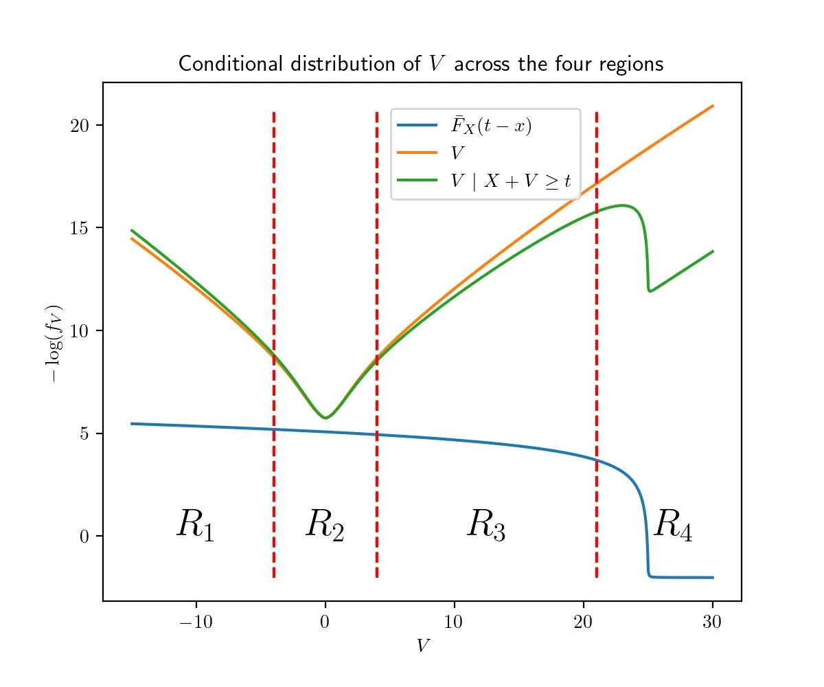
Note that up to a constant vertical shift of normalization, the green curve is the pointwise sum of the blue and orange curves.

B.1.2 Definitions

To be more precise, we’re going to make the following definitions and assumptions:

Let $f_{V}(v)$ be the PDF of $V$ at the value $v$. We assume for convenience that $f_{V}$ exists, is integrable, etc, though we suspect that this isn’t necessary, and that one could work through a similar proof just referring to the tails of $V$. We won’t make this assumption for $X$. Let $F_{X}(x)=\text{Pr}(X\leq x)$ and $\bar{F}_{X}(x)=\text{Pr}(X>x)$, similarly for $F_{V}$ and $\bar{F}_{V}$. Assume that

• $V$ has a finite mean: $\int_{-\infty}^{\infty}vf_{V}(v)\,dv$ converges absolutely.

• $X$ is subexponential.

Formally, this means that $\lim_{x\to\infty}\frac{\text{Pr}(X_{1}+X_{2}>x)}{\text{Pr}(X>x)}=2$. This occurs roughly whenever $X$ has tails that are heavier than $e^{-cx}$ for any $c$ and is reasonably well-behaved; counterexamples to the claim "long-tailed implies subexponential" exist, but they’re nontrivial to exhibit. Examples of subexponential distributions include log-normal distributions, anything that decays like a power law, the Pareto distribution,and distributions with tails asymptotic to $e^{-x^{a}}$ for any $0<a<1$.

We require for $V$ that its tail function is substantially lighter than X’s, namely that $\lim_{t\to\infty}\frac{t^{p}\bar{F}_{V}(t)}{\bar{F}_{X}(t)}=0$ for some $p>1$. (This implies that $\bar{F}_{V}(t)=O(\bar{F}_{X}(t)/t)$.)

With these definitions and assumptions, we can move on to the proof.

The unnormalized PDF of $V$ conditioned on $X+V\geq t$ is given by $f_{V}(v)\bar{F}_{X}(t-v)$. Its expectation is given by $\frac{\int_{-\infty}^{\infty}vf_{V}(v)\bar{F}_{X}(t-v)}{\int_{-\infty}^{\infty}f_{V}(v)\bar{F}_{X}(t-v)}$.

Meanwhile, the unconditional expectation of V is given by $\int_{-\infty}^{\infty}vf_{V}(v)$.

We’d like to show that these two expectations are equal in the limit for large $t$. To do this, we’ll introduce $Q(v)=\frac{\bar{F}_{X}(t-v)}{\bar{F}_{X}(t)}$. (More pedantically, this should really be $Q_{t}(v)$, which we’ll occasionally use where it’s helpful to remember that this is a function of $t$.)

For a given value of $t$, $Q(v)$ is just a scaled version of $\bar{F}_{X}(t-v)$, so the conditional expectation of $V$ is given by $\frac{\int_{-\infty}^{\infty}vf_{V}(v)Q(v)}{\int_{-\infty}^{\infty}f_{V}(v)Q(v)}$. But because $Q(0)=1$, the numerator and denominator of this fraction are (for small $v$ ) close to the unconditional expectation and $1$, respectively.

We’ll aim to show that for all $\epsilon>0,$ we have for sufficiently large $t$ that $\left|\int_{-\infty}^{\infty}vf_{V}(v)Q_{t}(v)-\int_{-\infty}^{\infty}vf_{V}(v)\right|<\epsilon$ and $\int_{-\infty}^{\infty}f_{V}(v)Q_{t}(v)\in[1-\epsilon,1+\epsilon]$, which implies (exercise) that the two expectations have limiting difference zero. But first we need some lemmas.

B.1.3 Lemmas

Lemma 6.

There is $h(t)$ depending on $F_{X}$ such that:

1. $\lim_{x\to\infty}h(t)=\infty$

2. $\lim_{t\to\infty}t-h(t)=\infty$

3. $\lim_{t\to\infty}\frac{\bar{F}_{X}(t-h(t))}{\bar{F}_{X}(t)}=1$

4. $\lim_{t\to\infty}\sup_{|v|\leq h(t)}|Q(v,t)-1|=0$.

Proof.

Lemma 2.19 from (Foss et al., 2013) implies that if $X$ is long-tailed (which it is, because subexponential implies long-tailed), then there is $h(t)$ such that condition (a) holds and $\bar{F}_{X}$ is $h$-insensitive; by Proposition 2.20 we can take $h$ such that $h(t)\leq t/2$ for sufficiently large $t$, implying condition (b). Conditions (c) and (d) follow from being $h$-insensitive. ∎

Lemma 7.

Suppose that $F_{X}$ is whole-line subexponential and $h$ is chosen as in Lemma 1. Also suppose that $\bar{F}_{V}(t)=O(\bar{F}_{X}(t)/t)$. Then $Pr[X+V>t,\ V>h(t),\ X>h(t)]=o(\bar{F}_{X}(t)/t).$

Proof.

This is a slight variation on lemma 3.8 from (Foss et al., 2013), and follows from the proof of Lemma 2.37. Lemma 2.37 states that

Lemma 2.37. Let $h$ be any increasing function on $\mathbb{R}^{+}$such that $h(x)\rightarrow\infty$. Then, for any distributions $F_{1},F_{2},G_{1}$, and $G_{2}$ on $\mathbb{R}$,

$$\limsup_{x\rightarrow\infty}\frac{\mathbb{P}\left\{\xi_{1}+\eta_{1}>x,\xi_{1}>h(x),\eta_{1}>h(x)\right\}}{\mathbb{P}\left\{\xi_{2}+\eta_{2}>x,\xi_{2}>h(x),\eta_{2}>h(x)\right\}}\leq\limsup_{x\rightarrow\infty}\frac{\overline{F_{1}}(x)}{\overline{F_{2}}(x)}\cdot\limsup_{x\rightarrow\infty}\frac{\overline{G_{1}}(x)}{\overline{G_{2}}(x)},$$

where $\xi_{1},\xi_{2},\eta_{1}$, and $\eta_{2}$ are independent random variables with respective distributions $F_{1},F_{2},G_{1}$ and $G_{2}$.

but it is actually proved that

$$\mathbb{P}\left\{\xi_{1}+\eta_{1}>x,\xi_{1}>h(x),\eta_{1}>h(x)\right\}\leq\\ \sup_{z>h(x)}\frac{\overline{F_{1}}(z)}{\overline{F_{2}}(z)}\cdot\sup_{z>h(x)}\frac{\overline{G_{1}}(z)}{\overline{G_{2}}(z)}\cdot{\mathbb{P}\left\{\xi_{2}+\eta_{2}>x,\xi_{2}>h(x),\eta_{2}>h(x)\right\}}.$$ (8)

If we let $F_{1}=F_{V},F_{2}=G_{1}=G_{2}=F_{X}$, then we get

$$\mathbb{P}\left\{X+V>t,X>h(t),V>h(t)\right\}\\ \leq\sup_{z>h(t)}\frac{\bar{F}_{V}(z)}{\bar{F}_{X}(z)}\sup_{z>h(t)}\frac{\bar{F}_{X}(z)}{\bar{F}_{X}(z)}{\mathbb{P}\left\{X+X^{\prime}>t,X>h(t),X^{\prime}>h(t)\right\}}\\ =\sup_{z>h(t)}\frac{\bar{F}_{V}(z)}{\bar{F}_{X}(z)}{\mathbb{P}\left\{X+X^{\prime}>t,X>h(t),X^{\prime}>h(t)\right\}}\\$$ (9)

where $X,X^{\prime}\sim F_{X}$. Multiplying by $t$, we have

$$t\mathbb{P}\left\{X\!+\!V>t,X\!>\!h(t),V\!>\!h(t)\right\}\leq\sup_{z>h(t)}\frac{t\bar{F}_{V}(z)}{\bar{F}_{X}(z)}{\mathbb{P}\left\{X\!+\!X^{\prime}>t,X\!>\!h(t),X^{\prime}\!>\!h(t)\right\}},$$ (10)

and because $h(t)\to\infty$ as $t\to\infty$ and $\bar{F}_{V}(t)=O(\bar{F}_{X}(t)/t)$, we can say that for some $c<\infty$, $\lim_{t\to\infty}\sup_{z>h(t)}\frac{t\bar{F}_{V}(z)}{\bar{F}_{X}(z)}<c$. Therefore for sufficiently large t $\mathbb{P}\left\{X+V>t,X>h(t),V>h(t)\right\}\leq\frac{c}{t}{\mathbb{P}\left\{X\!+\!X^{\prime}>t,X\!>\!h(t),X^{\prime}\!>\!h(t)\right\}}$.

By Theorem 3.6, $\mathbb{P}\left\{X\!+\!X^{\prime}>t,X\!>\!h(t),X^{\prime}\!>\!h(t)\right\}$ is $o(\bar{F}_{X}(t))$, so the LHS is $o(\bar{F}_{X}(t)/t)$ as desired. ∎

B.1.4 Bounds on the numerator

We want to show, for arbitrary $\epsilon>0$, that $\left|\int_{-\infty}^{\infty}vf_{V}(v)Q(v)-\int_{-\infty}^{\infty}vf_{V}(v)\right|<\epsilon$ in the limit as $t\to\infty$. Since $\left|\int_{-\infty}^{\infty}vf_{V}(v)Q(v)-\int_{-\infty}^{\infty}vf_{V}(v)\right|\leq\int_{-\infty}^{\infty}\left|vf_{V}(v)(Q(v)-1)\right|=\int_{-\infty}^{\infty}|v|\cdot f_{V}(v)\cdot|Q(v)-1|$ it will suffice to show that the latter quantity is less than $\epsilon$ for large $t$.

We’re going to show that $\int_{-\infty}^{\infty}|v|\cdot f_{V}(v)\cdot|Q(v)-1|$ is small by showing that the integral gets arbitrarily small on each of four pieces: $(-\infty,-h(t)]$, $(-h(t),h(t))$, $[h(t),t-h(t)]$, and $(t-h(t),\infty)$.

We’ll handle these case by case (they’ll get monotonically trickier).

Region 1: $(-\infty,-h(t)]$

Since $\int_{-\infty}^{\infty}vf_{V}(v)$ is absolutely convergent, for sufficiently large $t$ we will have $\int_{-\infty}^{-h(t)}|v|f_{V}(v)<\epsilon$, since $h(t)$ goes to infinity by Lemma 1(a).

Since $Q(v)$ is monotonically increasing and $Q(0)=1$, we know that in this interval $|Q(v)-1|=1-Q(v)$.

So we have $\int_{-\infty}^{-h(t)}|v|\cdot f_{V}(v)\cdot|Q(v)-1|=\int_{-\infty}^{-h(t)}|v|f_{V}(v)(1-Q(v))<\int_{-\infty}^{-h(t)}|v|f_{V}(v)<\epsilon$ as desired.

Region 2: $(-h(t),h(t))$

By lemma 1(d), $h$ is such that for sufficiently large $t$, $|Q(v)-1|<\frac{\epsilon}{\int_{-\infty}^{\infty}|v|f_{V}(v)}$ on the interval $[-h(t),h(t)]$. (Note that the value of this upper bound depends only on $V$ and $\epsilon$, not on $t$ or $h$.) So we have $\int_{-h(t)}^{h(t)}|v|f_{V}(v)|Q(v)-1|<\frac{\epsilon}{\int_{-\infty}^{\infty}|v|f_{V}(v)}\int_{-h(t)}^{h(t)}|v|f_{V}(v)<\frac{\epsilon}{\int_{-\infty}^{\infty}|v|f_{V}(v)}\int_{-\infty}^{\infty}|v|f_{V}(v)=\epsilon$.

Region 3: $[h(t),t-h(t)]$

For the third part, we’d like to show that $\int_{h(t)}^{t-h(t)}vf_{V}(v)(Q(v)-1)<\epsilon$. Since $\int_{h(t)}^{t-h(t)}vf_{V}(v)(Q(v)-1)<\int_{h(t)}^{t-h(t)}tf_{V}(v)Q(v)=\frac{t}{\bar{F}_{X}(t)}\int_{h(t)}^{t-h(t)}f_{V}(v)\bar{F}_{X}(t-v)$ it would suffice to show that the latter expression becomes less than $\epsilon$ for large $t$, or equivalently that $\int_{h(t)}^{t-h(t)}f_{V}(v)\bar{F}_{X}(t-v)=o\left(\frac{\bar{F}_{X}(t)}{t}\right)$.

The LHS in this expression is the unconditional probability that $X+V>t$ and $h(t)<V<t-h(t)$, but this event implies $X+V>t,V>h(t)$, and $X>h(t)$. So we can write

$$\int_{h(t)}^{t-h(t)}f_{V}(v)\bar{F}_{X}(t-v)=Pr[X+V>t,\ h(t)<V<t-h(t)]\\ <Pr[X+V>t,\ V>h(t),\ X>h(t)]=o(\bar{F}_{X}(t)/t)$$

by Lemma 2.

Region 4: $(t-h(t),\infty)$

For the fourth part, we’d like to show that $\int_{t-h(t)}^{\infty}vf_{V}(v)Q(v)\to 0$ forlarge $t$.

Since $Q(v)=\frac{\bar{F}_{X}(t-v)}{\bar{F}_{X}(t)}<\frac{1}{\bar{F}_{X}(t)}$, it would suffice to show $\int_{t-h(t)}^{\infty}vf_{V}(v)=o(\bar{F}_{X}(t))$. But note that since $\lim_{t\to\infty}\frac{\bar{F}_{X}(t-h(t))}{\bar{F}_{X}(t)}=1$ by Lemma 1(c), this is equivalent to $\int_{t-h(t)}^{\infty}vf_{V}(v)=o(\bar{F}_{X}(t-h(t)))$, which (by Lemma 1(b)) is equivalent to $\int_{t}^{\infty}vf_{V}(v)=o(\bar{F}_{X}(t))$.

Note that $\int_{t}^{\infty}vf_{V}(v)=t\int_{t}^{\infty}f_{V}(v)+\int_{t}^{\infty}(v-t)f_{V}(v)=t\bar{F}_{V}(t)+\int_{t}^{\infty}\bar{F}_{V}(v)$, so it will suffice to show that both terms in this sum are $o(\bar{F}_{X}(t))$.

The first term $t\bar{F}_{V}(t)$ is $o(\bar{F}_{X}(t))$ because we assumed $\lim_{t\to\infty}\frac{t^{p}\bar{F}_{V}(t)}{\bar{F}_{X}(t)}=0$ for some $p>1$.

For the second term, we have for the same reason $\int_{t}^{\infty}\bar{F}_{V}(v)<\int_{t}^{\infty}\frac{\bar{F}_{X}(v)}{v^{p}}=\bar{F}_{X}(t)\int_{t}^{\infty}v^{-p}=\frac{t^{1-p}}{p-1}\bar{F}_{X}(t)=o(\bar{F}_{X}(t))$.

B.1.5 Bounds on the denominator

For the denominator, we want to show that $\lim_{t\to\infty}\int_{-\infty}^{\infty}f_{V}(v)Q_{t}(v)=1=\int_{-\infty}^{\infty}f_{V}(v)$, so it’ll suffice to show $|\int_{-\infty}^{\infty}f_{V}(v)(Q_{t}(v)-1)|=o(1)$ as $t\to\infty$. Again, we’ll break up this integral into pieces, though they’ll be more straightforward than last time. We’ll look at $(-\infty,-h(t))$, $[-h(t),h(t)]$, and $(h(t),\infty)$.

• $|\int_{-\infty}^{-h(t)}f_{V}(v)(Q(v)-1)|=\int_{-\infty}^{-h(t)}f_{V}(v)(1-Q(v))<\int_{-\infty}^{-h(t)}f_{V}(v)$.

  • But since $h(t)$ goes to infinity, this left tail of the integral will contain less and less of $V$ ’s probability mass as $t$ increases.

• $|\int_{-h(t)}^{h(t)}f_{V}(v)(Q(v)-1)|\leq\int_{-h(t)}^{h(t)}f_{V}(v)|Q(v)-1|$

• $\leq\sup_{|v|\leq h(t)}|Q(v,t)-1|\int_{-h(t)}^{h(t)}f_{V}(v)\leq\sup_{|v|\leq h(t)}|Q(v,t)-1|$

  • By Lemma 1(d) we know that this goes to zero for large $t$.

• $|\int_{h(t)}^{\infty}f_{V}(v)(Q(v)-1)|=\int_{h(t)}^{\infty}f_{V}(v)(Q(v)-1)<\int_{h(t)}^{\infty}f_{V}(v)Q(v)$.

But for sufficiently large $t$ we have $h(t)>1$, so we obtain $\int_{h(t)}^{\infty}f_{V}(v)Q(v)<\int_{h(t)}^{\infty}vf_{V}(v)Q(v)<\int_{-\infty}^{\infty}vf_{V}(v)Q(v)=o(1)$ by the results of the previous section. This completes the proof.

B.2 Conditioning with light-tailed error produces arbitrarily high utility

Theorem 8.

Let $X,V$ be independent random variables such that $\lim_{t\to\infty}\frac{\bar{F}_{X}(t+1)}{\bar{F}_{X}(t)}=0$. (This implies that X has tails that are dominated by $e^{-cx}$ for any c, though it’s a slightly stronger claim because it requires that X not have large jumps in the decay of its tails.) Then for any V with a finite mean which has no upper bound, $\lim_{t\to\infty}\mathbb{E}[V|X+V>t]=\infty$.

Theorem 8 generalizes a consequence of the "Regressional Goodhart Identity" in (Gao et al., 2023).

Proof.

Let $\text{Pr}(V>c+1)=p>0$, which exists by our assumption that $V$ is unbounded.

Let $\mathbb{E}[V|V<c]=q$. (If this is undefined because the conditional has probability $0$, we’ll have the desired result anyway since then $V$ would always be at least $c$.)

Observe that for all $t$, $\mathbb{E}[V|V<c,X+V>t]\geq q$ (assuming it is defined), because we’re conditioning $(V|V<c)$ on an event which is more likely for larger $v$ (since $X$ and $V$ are independent).

First, let’s see that $\lim_{t\to\infty}\frac{P(V<c|X+V\geq t)}{P(V>c+1|X+V\geq t)}=0$. This ratio of probabilities is equal to

$\frac{\int_{-\infty}^{c}f_{V}(v)\bar{F}_{X}(t-v)}{\int_{c+1}^{\infty}f_{V}(v)\bar{F}_{X}(t-v)}\leq\frac{\int_{-\infty}^{c}f_{V}(v)\bar{F}_{X}(t-c)}{\int_{c+1}^{\infty}f_{V}(v)\bar{F}_{X}(t-c-1)}=\frac{\bar{F}_{X}(t-c)}{\bar{F}_{X}(t-c-1)}\cdot\frac{\int_{-\infty}^{c}f_{V}(v)}{\int_{c+1}^{\infty}f_{V}(v)}$

$=\frac{\bar{F}_{X}(t-c)}{\bar{F}_{X}(t-c-1)}\cdot\frac{\text{Pr}(V<c)}{\text{Pr}(V>c+1)}\leq\frac{\bar{F}_{X}(t-c)}{\bar{F}_{X}(t-c-1)}\cdot\frac{1}{p}$

which, by our assumption that $\lim_{t\to\infty}\frac{\bar{F}_{X}(t+1)}{\bar{F}_{X}(t)}=0$, will get arbitrarily small as $t$ increases for any positive $p$.

Now, consider $\mathbb{E}[V|X+V\geq t]$. We can break this up as the sum across outcomes $Z$ of $\mathbb{E}[V|Z,X+V\geq t]\cdot\text{Pr}(Z|X+V\geq t)$ for the three disjoint outcomes $V<c$, $c\leq V\leq c+1$, and $V>c+1$. Note that we can lower bound these expectations by $q,c,c+1$ respectively. But then once $t$ is large enough that $\frac{\text{Pr}(V<c|X+V\geq t)}{\text{Pr}(V>c+1|X+V\geq t)}<\frac{1}{c-q}$, this weighted sum of conditional expectations will add to more than $c$. ∎

Appendix C Additional figures

See figures 5, 6.

Figure 5: Histogram and normal probability plot of reward assigned by Pythia RM to random length-1024 token sequences. The Q-Q plot suggests the distribution is approximately normal, which is much lighter-tailed than exponential.

Figure 6: Reward and log-probability for ACG-optimized inputs to Starling 7B-alpha.

Appendix D Hyperparameters for ACG

See table 2.

Table 2: Hyperparameters for ACG

Parameter	Value
Context length	133
Iterations	1000
Candidates per seq. position (k)	3
Annealing starting value	9
Annealing ending value	2

Appendix E Assets

We use three models for our experiments: Starling 7B-alpha, Llama 2 7B-chat, and Pythia-1.4B. Starling was developed by Berkeley, and Pythia by EleutherAI. Starling and Pythia models are licensed under Apache-2.0. Llama 2 models were developed by Meta and licensed under a license published by Meta.

References

- Abdolmaleki et al. (2018) Abdolmaleki, A., Springenberg, J. T., Tassa, Y., Munos, R., Heess, N., and Riedmiller, M. Maximum a posteriori policy optimisation. CoRR, 2018. URL http://arxiv.org/abs/1806.06920v1.
- Christiano et al. (2017) Christiano, P. F., Leike, J., Brown, T., Martic, M., Legg, S., and Amodei, D. Deep reinforcement learning from human preferences. In Guyon, I., Luxburg, U. V., Bengio, S., Wallach, H., Fergus, R., Vishwanathan, S., and Garnett, R. (eds.), Advances in Neural Information Processing Systems, volume 30. Curran Associates, Inc., 2017. URL https://proceedings.neurips.cc/paper_files/paper/2017/file/d5e2c0adad503c91f91df240d0cd4e49-Paper.pdf.
- Clark & Amodei (2016) Clark, J. and Amodei, D. Faulty reward functions in the wild, December 2016. URL https://openai.com/index/faulty-reward-functions/. Accessed: 2024-07-07.
- Foss et al. (2013) Foss, S., Korshunov, D., and Zachary, S. An Introduction to Heavy-Tailed and Subexponential Distributions. Springer, 2 edition, 2013. doi: 10.1007/978-1-4614-7101-1. URL https://link.springer.com/book/10.1007/978-1-4614-7101-1.
- Gao et al. (2023) Gao, L., Schulman, J., and Hilton, J. Scaling laws for reward model overoptimization. In Krause, A., Brunskill, E., Cho, K., Engelhardt, B., Sabato, S., and Scarlett, J. (eds.), Proceedings of the 40th International Conference on Machine Learning, volume 202 of Proceedings of Machine Learning Research, pp. 10835–10866. PMLR, 23–29 Jul 2023. URL https://proceedings.mlr.press/v202/gao23h.html.
- Haize Labs (2024) Haize Labs. Making a sota adversarial attack on llms 38x faster. https://blog.haizelabs.com/posts/acg/, March 2024. Accessed: 2024-05-22.
- Jaques et al. (2019) Jaques, N., Ghandeharioun, A., Shen, J. H., Ferguson, C., Lapedriza, A., Jones, N., Gu, S., and Picard, R. Way off-policy batch deep reinforcement learning of implicit human preferences in dialog. arXiv preprint arXiv:1907.00456, 2019.
- Laidlaw et al. (2024) Laidlaw, C., Singhal, S., and Dragan, A. Preventing reward hacking with occupancy measure regularization. arXiv, 2024. URL https://www.arxiv.org/abs/2403.03185. Accessed: 2024-07-07.
- Lambert & Calandra (2024) Lambert, N. and Calandra, R. The alignment ceiling: Objective mismatch in reinforcement learning from human feedback, feb 2024.
- Lambert et al. (2023) Lambert, N., Pyatkin, V., Morrison, J., Miranda, L., Lin, B. Y., Chandu, K., Dziri, N., Kumar, S., Zick, T., Choi, Y., Smith, N. A., and Hajishirzi, H. Rewardbench: Evaluating reward models for language modeling, 2023. URL https://arxiv.org/abs/2403.13787. 40 pages, 19 figures, 12 tables.
- Schulman et al. (2015) Schulman, J., Levine, S., Moritz, P., Jordan, M. I., and Abbeel, P. Trust region policy optimization. CoRR, 2015. URL http://arxiv.org/abs/1502.05477v5.
- Schulman et al. (2017) Schulman, J., Wolski, F., Dhariwal, P., Radford, A., and Klimov, O. Proximal policy optimization algorithms. CoRR, 2017. URL http://arxiv.org/abs/1707.06347v2.
- Wierman (2013) Wierman, A. Catastrophes, conspiracies, and subexponential distributions (part ii). https://rigorandrelevance.wordpress.com/2013/12/17/catastrophes-conspiracies-and-subexponential-distributions-part-ii/, 2013. Accessed: 2024-06-26.
- Zhu et al. (2023) Zhu, B., Frick, E., Wu, T., Zhu, H., and Jiao, J. Starling-7B: Improving llm helpfulness & harmlessness with rlaif, November 2023.
- Zhuang & Hadfield-Menell (2021) Zhuang, S. and Hadfield-Menell, D. Consequences of misaligned AI. Advances in Neural Information Processing Systems, 33:15762–15773, 2021. doi: 10.48550/arXiv.2102.03896. URL https://arxiv.org/abs/2102.03896. arXiv:2102.03896v1 [cs.AI].
- Ziegler et al. (2020) Ziegler, D. M., Stiennon, N., Wu, J., Brown, T. B., Radford, A., Amodei, D., Christiano, P., and Irving, G. Fine-tuning language models from human preferences, 2020. URL https://arxiv.org/abs/1909.08593. arXiv:1909.08593v2 [cs.CL].
- Zou et al. (2023) Zou, A., Wang, Z., Kolter, J. Z., and Fredrikson, M. Universal and transferable adversarial attacks on aligned language models, 2023.