Decomposed Direct Preference Optimization for Structure-Based Drug Design

Abstract

Diffusion models have achieved promising results for Structure-Based Drug Design (SBDD). Nevertheless, high-quality protein subpocket and ligand data are relatively scarce, which hinders the models’ generation capabilities. Recently, Direct Preference Optimization (DPO) has emerged as a pivotal tool for the alignment of generative models such as large language models and diffusion models, providing greater flexibility and accuracy by directly aligning model outputs with human preferences. Building on this advancement, we introduce DPO to SBDD in this paper. We tailor diffusion models to pharmaceutical needs by aligning them with elaborately designed chemical score functions. We propose a new structure-based molecular optimization method called DecompDpo, which decomposes the molecule into arms and scaffolds and performs preference optimization at both local substructure and global molecule levels, allowing for more precise control with fine-grained preferences. Notably, DecompDpo can be effectively used for two main purposes: (1) fine-tuning pretrained diffusion models for molecule generation across various protein families, and (2) molecular optimization given a specific protein subpocket after generation. Extensive experiments on the CrossDocked2020 benchmark show that DecompDpo significantly improves model performance in both molecule generation and optimization, with up to 100% Median High Affinity and a 54.9% Success Rate.

1 Introduction

Structure-based drug design (SBDD) [2] is a strategic approach in medicinal chemistry and pharmaceutical research that utilizes 3D structures of biomolecules to guide the design and optimization of new therapeutic agents. The goal of SBDD is to design molecules that bind to given protein targets. Recently, some researchers view this problem as a conditional generative task in a data-driven way, and introduced powerful generative models equipped with geometric deep learning [27]. For example, Peng et al. [26], Zhang and Liu [39] proposed to generate the atoms or fragments sequentially by a SE(3)-equivariant auto-regressive model, while Luo et al. [23], Peng et al. [26], Guan et al. [12] introduced diffusion models [16] to model the distribution of types and positions of ligand atoms. However, the scarcity of high-quality protein-ligand pair data has emerged as a significant bottleneck for the development of generative models in SBDD [35]. Typically, the success of deep learning relies on the foundation of large-scale datasets. The growth of the Internet and social media, alongside the convenience of modern recording devices, has greatly simplified the collection of text, images, and videos. This has rapidly accelerated the advancement of deep learning within the realms of computer vision and natural language processing. However, the collection of protein-ligand binding data is challenging and limited due to the complex and resource-intensive experimental procedures. Notably, CrossDocked2020 dataset [10], the widely-used dataset for SBDD, consists of ligands that are docked into multiple similar binding pockets across the Protein Data Bank using docking software. This may be regarded as a form of data augmentation; while it expands the dataset’s size, it may unavoidably introduce some low-quality data. Besides, the number of unique ligands remain the same before and after this data augmentation. As Zhou et al. [41] highlight, the ligands in CrossDocked2020 dataset have moderate binding affinities, which do not meet the stringent demands of drug design.

To address the aforementioned challenge, Xie et al. [37], Fu et al. [11] provides a straightforward method for searching molecules with desired properties in the extensive chemical space. However, pure searching or optimization methods lack generative capabilities and fall short in the diversity of the designed molecules. Zhou et al. [41] integrated conditional diffusion models with iterative optimization by providing molecular substructures as conditions of conditional diffusion models and iteratively replacing the substructures with better ones. This method achieves better properties and maintains certain diversity. Nonetheless, the performance of this method is still limited due to fixed model parameters during the optimization process.

To break the bottleneck, we propose to fine-tune diffusion models for SBDD to align with the practical pharmaceutical needs. Recent years have witnessed huge success achieved by large language models (LLMs) [1, 34]. Reinforcement learning from human/AI feedback (RLHF/RLAIF) [43, 33, 24, 20, 3] was proposed to align large language models to human preference and improve the users’ satisfaction. Typical RLHF requires explicit reward modeling, while Direct Preference Optimization (DPO) [28] directly fine-tunes LLMs on human preference data, which significantly simplifies the procedures and still leads to remarkable improvements. This motivates us to propose DecompDpo, a method of fine-tuning diffusion models for SBDD with DPO to align them with practical requirements of drug discovery. Specifically, we use pretrained DecompDiff [13], a strong diffusion-based generative model for SBDD, as the base model to synthesize massive molecules and use comprehensive in silico evaluation to obtain preference data. We introduce Diffusion-DPO [36] to optimize non-deomposable properties of ligand molecules generated by diffusion models. We named this method as GlobalDPO. Inspired by the decomposition nature of ligand molecules when they bind to proteins, for the properties that are decomposable (e.g, binding affinity, which is measured by Vina [7]), we propose decomposed DPO loss, termed as LocalDPO, where we define preferences over substructures instead of the whole molecules. Additionally, we propose linear beta schedule which also improves the performance remarkedly. We apply our method to two scenarios: structure-based molecular generation and structure-based molecular optimization. Under both setting, our method can significantly outperform baselines, demonstrating its flexibility and effectiveness. We highlight our contributions as follows:

• We propose DecompDpo, consisting of GlobalDPO and LocalDPO for optimizing non-decomposable and decomposable properties, respectively. In LocalDPO, we introduce decomposition to DPO loss which improve its effectiveness and flexibility.

• Our approaches are applicable to both structure-based molecular generation and optimization. Notably, DecompDpo achieves 100% Median High Affinity and a 54.9% Success Rate on CrossDocked2020 dataset.

• To the best of our knowledge, we are the first to introduce preference alignment to structure-based drug design. Our approaches align the generative models for SBDD with the practical requirements of drug discovery.

2 Related Work

Structure-based Drug Design

Structure-based drug design (SBDD) aims to design ligand molecules that can bind to specific protein targets. Recent efforts have been made to enhance the efficiency of generating molecules with desired properties. Ragoza et al. [29] employed variational autoencoder to generate 3D molecules in atomic density grids. Luo et al. [23], Peng et al. [26], Liu et al. [22] adopted an autoregressive approach to generate 3D molecules atom by atom, while Zhang et al. [40] proposed to generate 3D molecules by predicting a series of molecular fragments in an auto-regressive way. Guan et al. [12], Schneuing et al. [30], Lin et al. [21] introduced diffusion models to SBDD, which first generate the types and positions of atoms and subsequently determine bond types by post-processing. Some recent studies have sought to further improve efficacy of SBDD methods by incorporating biochemical prior knowledge. DecompDiff [13] proposed decomposing ligands into substructures and generating atoms and bonds simultaneously using diffusion models with decomposed priors and validity guidance. DrugGPS [39] considered subpocket-level similarities, augmenting molecule generation through global interaction between subpocket prototypes and molecular motifs. IPDiff [17] addressed the inconsistency between forward and reverse processes using a pre-trained protein-ligand interaction prior network. In addition to simply generative modeling of existing protein-ligand pairs, some researchers leveraged optimization algorithms to design molecules with desired properties. AutoGrow 4 [32] and RGA [11] optimized the binding affinity of ligand molecules towards specific targets by elaborate genetic algorithms. RGA [11] viewed the evolutionary process as a Markov decision process and guided it by reinforcement learning. DecompOpt [41] proposed a controllable and decomposed diffusion model that can generate ligand molecules conditioning on both protein subpockets and reference substructures, and combined it with iterative optimization to improve desired properties by iteratively generating molecules given substructures observed in previous iterations. Our work also focuses on designing molecules with desired properties by optimization. Differently, we optimize the parameters of the model that generate molecules instead of molecules themselves, which has been demonstrated to be more effective and efficient.

Learning from Human/AI Feedback Maximizing likelihood optimization of generative models cannot always satisfy users’ preferences. Thus introducing human or AI assessment to improve the performance of generative models has attracted significant attention. Reinforcement learning from human/AI feedback [43, 33, 24, 20, 3] was proposed to align large language models to human preference, consisting of reward modeling from comparison data annotated by human or AI and then using policy-gradient methods [6, 31] to fine-tune the model to maximize the reward. Similar techniques have also been introduced to diffusion models for text-to-image generation [5, 9, 38], where the generative process is viewed as a multi-step Markov decision process and policy-gradient methods can be then applied to fine-tuning the models. Recently, Direct Preference Optimization (DPO) [28], which aligns large language models to human preferences by directly optimizing on human comparison data, has attracted much attention. Wallace et al. [36] re-formulated DPO and derived Diffusion-DPO for aligning text-to-image diffusion models. The above works focus on aligning large language models or text-to-image diffusion models with human preferences. Recently, Zhou et al. [42] proposed to fine-tune diffusion models for antibody design by DPO and choose low Rosetta energy as preference. In our work, we introduce preference alignment to improve the desired properties of generated molecules given specific protein pockets and propose specialized methods to improve the performance of DPO in the scenario of SBDD.

3 Method

In this section, we will present our method, DecompDpo, as illustrated in Figure 1. In Section 3.1, we define the SBDD task and introduce the decomposed diffusion model for this task. Then, in Section 3.2, we describe the alignment of pre-trained diffusion models with preferences defined within the decomposed space, highlighting how DecompDpo’s multi-granularity control enhances the effectiveness and flexibility of the optimization. In Section 3.3, we develop a linear beta schedule for regularization to improve the optimization efficiency.

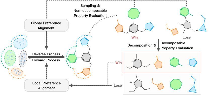
Figure 1: Illustration of DecompDpo. (a) molecules are generated using a pre-trained diffusion model. (b) For each molecule, non-decomposable properties are evaluated. Preference pairs are then constructed from these evaluations and used in global preference alignment. (c) Each molecule is further decomposed into substructures, and decomposable properties are evaluated at substructure level. These properties are used to construct local preferences, which are aligned using LocalDPO.

3.1 Preliminaries

In the context of SBDD, generative models are conditioned on the protein binding site, represented as $\mathcal{P}=\{({\bm{x}}_{i}^{\mathcal{P}},{\bm{v}}_{i}^{\mathcal{P}})\}_{i\in\{1,\cdots,N_{\mathcal{P}}\}}$, to generate ligands $\mathcal{M}=\{({\bm{x}}_{i}^{\mathcal{M}},{\bm{v}}_{i}^{\mathcal{M}},{\bm{b}}_{ij}^{\mathcal{M}})\}_{i,j\in\{1,\cdots,N_{\mathcal{M}}\}}$ that bind to this site. Here, $N_{\mathcal{P}}$ and $N_{\mathcal{M}}$ are the number of atoms in the protein and ligand, respectively. For both proteins and ligands, ${\bm{x}}\in{\mathbb{R}}^{3},{\bm{v}}\in{\mathbb{R}}^{h},{\bm{b}}_{ij}\in{\mathbb{R}}^{5}$ represents the coordinates of atoms, the types of atoms, and the bonds between atoms. Here we consider $h$ types of atoms (i.e., H, C, N, O, S, Se) and 5 types of bonds (i.e., non-bond, single, double, triple, aromatic).

Following the decomposed diffusion model introduced by Guan et al. [13], each ligand is decomposed into fragments $\mathcal{K}$, comprising several arms $\mathcal{A}$ connected by at most one scaffold $\mathcal{S}$ ($|{\mathcal{A}}|\geq 1,|{\mathcal{S}}|\leq 1,K=|{\mathcal{K}}|=|{\mathcal{A}}|+|{\mathcal{S}}|$). Based on the decomposed substructures, informative data-dependent priors ${\mathbb{O}}_{\mathcal{P}}=\{{\bm{\mu}}_{1:K},{\bm{\Sigma}}_{1:K},{\mathbf{H}}\}$ are estimated from atom positions by maximum likelihood estimation. This data-dependent prior enhances the training efficacy of the diffusion model, where $\mathcal{M}$ is gradually diffused with a fixed schedule $\{\lambda_{t}\}_{t=1,\cdots,T}$. We denote $\alpha_{t}=1-\lambda_{t}$ and $\bar{\alpha}_{t}=\prod_{s=1}^{t}\alpha_{t}$. The $i$-th atom position is shifted to its corresponding prior center: $\tilde{{\mathbf{x}}}_{t}^{i}={\mathbf{x}}_{t}^{i}-({\mathbf{H}}^{i})^{\top}{\bm{\mu}}$. The noisy data distribution at time $t$ derived from the distribution at time $t-1$ is computed as follows:

$$p(\tilde{{\mathbf{x}}}_{t}|\tilde{{\mathbf{x}}}_{t-1},\mathcal{P}) =\prod_{i=1}^{N_{\mathcal{M}}}\mathcal{N}(\tilde{{\mathbf{x}}}_{t}^{i};\tilde{{\mathbf{x}}}_{t-1}^{i},\lambda_{t}({\mathbf{H}}^{i})^{\top}{\bm{\Sigma}}),$$ (1)

$$p({\mathbf{v}}_{t}|{\mathbf{v}}_{t-1},\mathcal{P}) =\prod_{i=1}^{N_{\mathcal{M}}}\mathcal{C}({\mathbf{v}}_{t}^{i}|(1-\lambda_{t}){\mathbf{v}}_{t-1}^{i}+\lambda_{t}/K_{a}),$$ (2)

$$p({\mathbf{b}}_{t}|{\mathbf{b}}_{t-1},\mathcal{P}) =\prod_{i=1}^{N_{\mathcal{M}}\times N_{\mathcal{M}}}\mathcal{C}({\mathbf{b}}_{t}^{i}|(1-\lambda_{t}){\mathbf{b}}_{t-1}^{i}+\lambda_{t}/K_{b}),$$ (3)

where $K_{a}$ and $K_{b}$ represent the number of atom types and bond types used for featurization. The perturbed structure is then fed into the prediction model, then the reconstruction loss at the time $t$ can be derived from the KL divergence as follows:

$$L^{(x)}_{t}=||{\mathbf{x}}_{0}-\hat{{\mathbf{x}}}_{0}||^{2},\ L^{(v)}_{t}=\sum_{k=1}^{K_{a}}\bm{c}({\mathbf{v}}_{t},{\mathbf{v}}_{0})_{k}\log\frac{\bm{c}({\mathbf{v}}_{t},{\mathbf{v}}_{0})_{k}}{\bm{c}({\mathbf{v}}_{t},\hat{\mathbf{v}}_{0})_{k}},\ L^{(b)}_{t}=\sum_{k=1}^{K_{b}}\bm{c}({\mathbf{b}}_{t},{\mathbf{b}}_{0})_{k}\log\frac{\bm{c}({\mathbf{b}}_{t},{\mathbf{b}}_{0})_{k}}{\bm{c}({\mathbf{b}}_{t},\hat{\mathbf{b}}_{0})_{k}},$$

where $({\mathbf{x}}_{0},{\mathbf{v}}_{0},{\mathbf{b}}_{0})$, $({\mathbf{x}}_{t},{\mathbf{v}}_{t},{\mathbf{b}}_{t})$, $(\hat{{\mathbf{x}}}_{0},\hat{{\mathbf{v}}}_{0},\hat{{\mathbf{b}}}_{0})$, represent true atoms positions, types, and bonds types at time $0$, time $t$, predicted atoms positions, types, and bonds types at time $t$; $\bm{c}$ denotes mixed categorical distribution with weight $\bar{\alpha}_{t}$ and $1-\bar{\alpha}_{t}$. The overall loss is $L_{t}=L^{(x)}_{t}+\gamma_{v}L^{(v)}_{t}+\gamma_{b}L^{(b)}_{t}$, with $\gamma_{v},\gamma_{b}$ as weights of reconstruction loss of atom and bond type. We provide more details for the model architecture in Appendix B. To better illustrate decomposition, we show a decomposed molecule with the arms highlighted in Figure 2.

3.2 Direct Preference Optimization in Decomposed Space

Despite the diffusion models achieving promising results in modeling existing molecules, it may fail to meet the practical goal of SBDD is to synthesize molecules with the desired properties. By maximizing the reward function, the pre-learned model distribution can be optimized towards regions of higher quality. Drawing on RLHF, we formulate this optimization problem in SBDD as follows:

$$\underset{p_{\theta}}{\max}\ \mathbb{E}_{{\mathcal{P}}\sim{\mathcal{D}},{\mathcal{M}}\sim p_{\theta}({\mathcal{M}}\mid{\mathcal{P}})}r({\mathcal{M}},{\mathcal{P}})-\beta{\mathbb{D}}_{\text{KL}}\left[p_{\theta}({\mathcal{M}}\mid{\mathcal{P}})\parallel p_{\text{ref}}({\mathcal{M}}\mid{\mathcal{P}})\right],$$ (4)

where ${\mathcal{D}}$ is the distribution of the training set, $r({\mathcal{M}},{\mathcal{P}})$ is the reward function that evaluates properties of generated molecules, and $\beta>0$ is a hyperparameter for the Kullback–Leibler (KL) divergence regularization, which controls the derivation from the reference model $p_{\text{ref}}$. Following DPO proposed by Rafailov et al. [28], by leveraging preference data pair $({\mathcal{M}}^{+},{\mathcal{M}}^{-})$ with superior and inferior properties, the DPO training loss is expressed as follows:

$${\mathcal{L}}_{\text{DPO}}=-\mathbb{E}_{({\mathcal{P}},{\mathcal{M}}^{+},{\mathcal{M}}^{-})\sim{\mathcal{D}}}\ \text{log}\sigma\bigg{(}\beta\text{log}\frac{p_{\theta}({\mathcal{M}}^{+}\mid{\mathcal{P}})}{p_{\text{ref}}({\mathcal{M}}^{+}\mid{\mathcal{P}})}-\beta\text{log}\frac{p_{\theta}({\mathcal{M}}^{-}\mid{\mathcal{P}})}{p_{\text{ref}}({\mathcal{M}}^{-}\mid{\mathcal{P}})}\bigg{)}.$$ (5)

Wallace et al. [36] borrows the idea of DPO in LLM, proposing Diffusion-DPO, which can directly optimize the distribution learned by diffusion models with the preference defined over the entire diffusion process. We turn this preference in SBDD as $r({\mathcal{M}},{\mathcal{P}})=\mathbb{E}_{p_{\theta}({\mathcal{M}}_{1:T}\mid{\mathcal{M}}_{0},{\mathcal{P}})}[R({\mathcal{M}}_{1:T},{\mathcal{P}})]$. Here, ${\mathcal{M}}_{1:T}$ denotes the diffusion trajectories from the reverse process $p_{\theta}^{*}$. The training loss for Diffusion-DPO is defined to capture the differences in rewards across these trajectories:

where ${\mathcal{M}}_{1:T}^{+}$ and ${\mathcal{M}}_{1:T}^{-}$ represent trajectories of molecules with superior and inferior properties, respectively. By leveraging Jensen’s inequality to externalize the expectation and replacing $p_{\theta}^{*}$ by $q$, the training loss for Diffusion-DPO is then reformulated as:

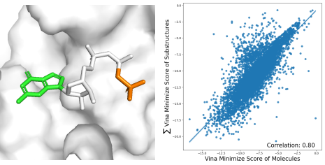
Figure 2: Example of molecule decomposition, with decomposed arms highlighted in green and orange (left). Person correlation coefficients between Vina Minimize Score of molecules and summation from its corresponding substructures (right).

Decomposable Optimization

Our next intuition is that the introduction of decomposition not only induced better evidence lower bound for diffusion model [13], but also showed potential in molecular optimization with a controllable diffusion model [41]. We notice that different molecular substructures, especially decomposed arms, can independently contribute to specific properties such as binding affinities and clash scores [15]. As illustrated in Figure 2, the Vina Minimize Score of molecules highly correlates with the summation of contributions from decomposed substructures.

Leveraging the above observation, we propose to extend the decomposition concept to preference optimization with diffusion models. Specifically, in DecompDpo, we construct preference pairs at the substructure level for objectives that can be decomposed and perform local preference alignment with LocalDPO, which will be introduced in detail below. Such substructure-level preference is more precise and can provide more flexibility, thus potentially improving the optimization efficacy. For properties that are inherently non-decomposable, we still use the molecule-level preference and perform global preference alignment with Diffusion-DPO, which we term as GlobalDPO below.

LocalDPO

Since certain optimization objectives, like Vina Minimize Score, can be calculated as summations of contributions from different substructures, we integrate decomposition into Diffusion-DPO and reformulate the training loss as follows:

where ${\mathcal{M}}^{(i)}$ represents the $i$-th decomposed substructure. In Diffusion-DPO, the preferences assigned to decomposed substructures are derived holistically from the preferences of the molecules. In other words, $+$ and $-$ in the substructure indicate that it is decomposed from the winning or losing molecule, regardless of its own properties.

We further introduce to construct preference pairs directly with substructures’ properties and define the training loss of LocalDPO as:

In Equation 9, $r({\mathcal{M}}^{(i)})$ represents the reward of the decomposed substructure ${\mathcal{M}}^{(i)}$ evaluated at time 0. We refer $A^{(i)}$ defined in Equation 9 as the preference learned by the model. The advantage of LocalDPO becomes evident when considering the consistency of substructure preferences with overall molecular preferences. When there exists a conflict, that is, if $r({\mathcal{M}}^{(i)+})<r({\mathcal{M}}^{(i)-})$, LocalDPO adjusts accordingly: if the preference learned by the model is consistent with the preference defined with substructures ($A^{(i)}<0$, $\text{sign}(\cdot)<0$), this results in a larger summation within $-\text{log}\sigma$, leading to a smaller loss because $-\text{log}\sigma$ is monotonically decreasing. Conversely, if the preference learned by the model is inconsistent with the preference defined with substructures ($A^{(i)}>0$, $\text{sign}(\cdot)<0$), it will result in a larger loss. In extreme cases, where the preference learned by the model invariably opposes the preferences of substructures, LocalDPO sets an upper bound for Diffusion-DPO.

Thanks to the GlobalDPO and LocalDPO introduced above, we are now able to integrate preferences across different granularities for effective multi-objective optimization. The final objective for DecompDpo can be expressed as follows:

$${\mathcal{L}}_{\text{{DecompDpo}}}=\sum_{q\in{\mathcal{Q}}_{\text{Decomp}}}{\mathcal{L}}_{\textsc{LocalDPO}}(q)+\sum_{q\in{\mathcal{Q}}_{\text{Non-Decomp}}}{\mathcal{L}}_{\textsc{GlobalDPO}}(q),$$ (10)

where ${\mathcal{Q}}_{\text{Decomp}}$ and ${\mathcal{Q}}_{\text{Non-Decomp}}$ represent the set of decomposable and non-decomposable properties, separately. We use LocalDPO to optimize decomposable properties and GlobalDPO to optimize non-decomposable properties. Such a dual granularity allows for more precise control over the optimization process and provides greater flexibility in selecting preferences to meet the diverse needs of molecular design.

3.3 Linear Beta Schedule

In diffusion models, the final steps of the reverse process play a crucial role, as they determine the types and positions of the atoms, thereby directly influencing the properties of generated molecules. These steps are also important for optimization, as achieving improved property distributions requires effective alignment with the desired properties. We propose a linear beta schedule to improve optimization efficiency and better balance the exploration of novel molecular structures with the adherence to pre-learned prior distribution. At each time step $t$, the schedule $\beta_{t}$ is defined as $\beta_{t}=\frac{t}{T}\beta_{T}$, where $\beta_{T}$ is the initial beta parameter defined at the last time step $T$. This progressive scaling reduces the regularization impact of the reference model during the crucial steps of the diffusion process, allowing the model to better align with preferences.

4 Experiments

Considering the practical demands of the pharmaceutical industry, we implement DecompDpo to meet two critical needs: (1) fine-tuning the reference model for broad molecule generation across various protein families, and (2) specifically optimizing the reference model for targeted protein subpockets. To assess the utility of DecompDpo, we first evaluate its ability to enhance molecule generation capabilities and benchmark its performance against representative generative models. We then examine DecompDpo’s effectiveness in navigating and adapting to distributions that exhibit desired properties for specific targets and compare it to recent optimization methods.

4.1 Experimental Setup

Dataset

Following previous work [23, 26, 12, 13], we use the CrossDocked2020 dataset [10] to pre-train our base model and to evaluate the performance of DecompDpo. Following the protocol established by Luo et al. [23], we filtered complexes to retain only those with high-quality docking poses (RMSD $<1$Å) and diverse protein sequences (sequence identity $<30\%$), resulting in a refined dataset comprising 100,000 high-quality training complexes and 100 novel proteins for evaluation.

Baselines

We compare DecompDpo with both generative methods and optimization methods. For generative methods, liGAN [29] employs a CNN-based variational autoencoder to encode both ligand and receptor into a latent space, subsequently generating atomic densities for ligands. Atom-based autoregressive models such as AR [23], Pocket2Mol [26], and GraphBP [22] update atom embeddings using a graph neural network (GNN). TargetDiff [12] and DecompDiff [13] utilize GNN-based diffusion models, the latter innovatively incorporates decomposed priors for predicting atoms’ type, position, and bonds with validity guidance. For optimization methods, we consider two strong baselines: RGA [11], which utilizes a reinforced genetic algorithm to simulate evolutionary processes and optimize a policy network across iterations, and DecompOpt [41], which leverages decomposed priors to control and optimize conditions in a diffusion model.

Evaluation

Following the methodology outlined by Guan et al. [12], we evaluate molecules from two aspects: target binding affinity and molecular properties, and molecular conformation. To assess target binding affinity, we use AutoDock Vina [7], following the established protocol from previous studies [23, 29]. Vina Score quantifies the direct binding affinity between a molecule and the target protein, Vina Min measures the affinity after local structural optimization via force field, Vina Dock assesses the affinity after re-docking the ligand into the target protein, and High Affinity measures the proportion of generated molecules with a Vina Dock score higher than that of the reference ligand. Regarding molecular properties, we calculate drug-likeness (QED) [4], synthetic accessibility (SA) [8], and diversity. The overall quality of generated molecules is evaluated by Success Rate (QED $>$ 0.25, SA $>$ 0.59, Vina Dock $<$ -8.18), following the defination in Jin et al. [18], Xie et al. [37]. To evaluate molecular conformation, Jensen-Shannon divergence (JSD) is employed to compare the atom distributions of the generated molecules with those of reference ligands. We also evaluate median energy difference of rigid fragments before and after optimizing molecules’ conformations with Merck Molecular Force Field (MMFF) [14].

Table 1: Summary of different properties of reference molecules and molecules generated by our method and other generative models and optimizaiton methods. ($\uparrow$) / ($\downarrow$) denotes a larger / smaller number is better. Top 2 results are highlighted with bold text and underlined text, respectively.

Methods Vina Score ($\downarrow$) Vina Min ($\downarrow$) Vina Dock ($\downarrow$) High Affinity ($\uparrow$) QED ($\uparrow$) SA ($\uparrow$) Diversity ($\uparrow$) Success Avg. Med. Avg. Med. Avg. Med. Avg. Med. Avg. Med. Avg. Med. Avg. Med. Rate ($\uparrow$) Reference -6.36 -6.46 -6.71 -6.49 -7.45 -7.26 - - 0.48 0.47 0.73 0.74 - - 25.0% Generate LiGAN - - - - -6.33 -6.20 21.1% 11.1% 0.39 0.39 0.59 0.57 0.66 0.67 3.9% GraphBP - - - - -4.80 -4.70 14.2% 6.7% 0.43 0.45 0.49 0.48 0.79 0.78 0.1% AR -5.75 -5.64 -6.18 -5.88 -6.75 -6.62 37.9% 31.0% 0.51 0.50 0.63 0.63 0.70 0.70 7.1% Pocket2Mol -5.14 -4.70 -6.42 -5.82 -7.15 -6.79 48.4% 51.0% 0.56 0.57 0.74 0.75 0.69 0.71 24.4% TargetDiff -5.47 -6.30 -6.64 -6.83 -7.80 -7.91 58.1% 59.1% 0.48 0.48 0.58 0.58 0.72 0.71 10.5% DecompDiff* -5.96 -7.05 -7.60 -7.88 -8.88 -8.88 72.3% 87.0% 0.45 0.43 0.60 0.60 0.60 0.60 28.0% DecompDpo -3.39 -7.08 -7.50 -8.04 -9.11 -9.22 79.0% 93.8% 0.48 0.46 0.64 0.64 0.62 0.61 36.9% Optimize RGA - - - - -8.01 -8.17 64.4% 89.3% 0.57 0.57 0.71 0.73 0.41 0.41 46.2% DecompOpt -5.87 -6.81 -7.35 -7.72 -8.98 -9.01 73.5% 93.3% 0.48 0.45 0.65 0.65 0.60 0.61 52.5% DecompDpo -2.83 -7.33 -7.23 -8.45 -9.89 -9.69 85.6% 100.0% 0.48 0.46 0.63 0.64 0.61 0.62 54.9%

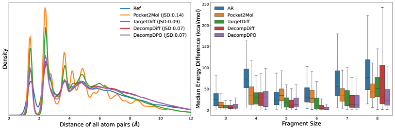
Figure 3: Compare pairwise distance distributions between all atoms in generated molecules and reference molecules from the test set. Jensen-Shannon divergence (JSD) between two distributions is reported (left). Median energy difference for rigid fragments of generated molecules before and after optimizing with the Merck Molecular Force Field (right).

Implementation Details

The bond-first noise schedule proposed by Peng et al. [25] effectively addresses the common problem of inconsistency between atoms and bonds when using predicted bonds for molecule reconstruction. Since DecompDiff also reconstructs molecules with predicted bonds, we adapt this noise schedule for DecompDiff to develop an enhanced model. As shown in Table 1, this model demonstrates improved performance. Believing in the broad applicability of this schedule, we postulate that the bond first noise schedule can benefit optimization effectiveness and choose the enhanced DecompDiff as the starting point for DecompDpo. For more details about the bond first noise schedule, please refer to Appendix B.2. We select QED, SA, and Vina Minimize Score as our primary optimization objectives. Since QED and SA are inherently non-decomposable, we use molecule-level preference for optimizing these properties. Vina Minimize Score is decomposed to construct substructure-level preference for optimization. For molecule generation, we use the enhanced DecompDiff to generate 10 molecules and select the molecule with the highest and the lowest score for each protein in the training set. For protein-specific optimization, we use the model fine-tuned with DecompDpo as reference model, generating 1000 molecules and select 100 molecules with the highest and lowest scores to construct preference pairs for each protein. We select the checkpoint with the best performance for evaluation. For each target, 100 molecules are evaluated for all generative models, and 20 molecules are evaluated for all optimization methods. Please refer to Appendix B.4 for more details.

4.2 Main Results

First, we evaluate the model fine-tuned with DecompDpo against representative generative models in terms of molecular conformation. As illustrated in Figure 3 (a), DecompDpo has a comparable performance to DecompDiff, achieving the lowest JSD relative to the distribution of reference molecules among all generative models. Furthermore, as observed in Figure 3 (b), DecompDpo performs comparably to DecompDiff for molecules with fewer rotatable bonds and achieves lower energy differences for molecules with more rotatable bonds. These results highlight DecompDpo’s ability to accurately capture reasonable molecular conformations while effectively optimizing for desired molecular properties. We provide more evaluations of molecular conformations in Appendix C. We then evaluate the capability of DecompDpo in terms of molecular properties and binding affinities for both molecule generation and optimization.

Molecule Generation

As illustrated in Table 1, after a single round of fine-tuning with DecompDpo, there is a significant improvement in all metrics, demonstrating the effectiveness of DecompDpo in enhancing the capabilities of generative models, except for the mean Vina Score and Vina Minimize Score. The observed decrease in these two metrics can be attributed to our choice of Vina Minimize Score as the optimization objective, which is calculated after local conformations optimized using a force field. Therefore, this objective may not take into account collisions between molecules and the protein. In addition, to assess the direct impact of DecompDpo on the model distribution, we disabled the validity guidance, a sampling technique used in DecompDiff, which might have intensified this issue. We further explore the influence of validity guidance in Section 4.3 to better understand its role in mitigating these challenges.

Table 2: Ablation study of decomposing DPO loss and linear beta weight on 40 randomly selected protein pockets. ($\uparrow$) / ($\downarrow$) denotes a larger / smaller number is better. The best result is highlighted with bold text.

Method Vina Score ($\downarrow$) Vina Min ($\downarrow$) Vina Dock ($\downarrow$) High Affinity ($\uparrow$) QED ($\uparrow$) SA ($\uparrow$) Diversity ($\uparrow$) Success Avg. Med. Avg. Med. Avg. Med. Avg. Med. Avg. Med. Avg. Med. Avg. Med. Rate ($\uparrow$) DecompDpo -7.82 -7.90 -9.15 -8.74 -9.65 -10.08 94.8% 100.0% 0.49 0.48 0.64 0.65 0.61 0.60 54.7% Molecule-level Dpo -7.57 -7.53 -8.95 -8.72 -9.90 -9.64 93.4% 100.0% 0.50 0.47 0.62 0.64 0.58 0.56 50.9% w/ Constant Beta Weight -7.29 -7.50 -8.62 -8.60 -9.60 -9.50 90.7% 100.0% 0.49 0.45 0.62 0.64 0.59 0.58 52.1%

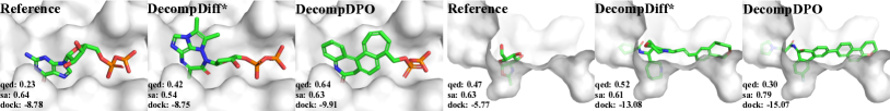
Figure 4: Visualization of reference binding ligands and the molecule with the highest property among all generated molecules of DecompDiff* and DecompDpo on protein 2HCJ (left column) and 1H0I (right column).

Molecule Optimization

Table 1 highlights DecompDpo’s outstanding performance, achieving the highest scores in most affinity-related metrics and the Success Rate. All optimization methods aim to explore the upper performance bound for each target, among which DecompDpo shows the strongest capability. Notably, unlike DecompOpt, which is constrained by a fixed conditional distribution learned from an existing dataset, DecompDpo benefits from an online learning paradigm. This approach uses feedback from generated molecules to optimize the distribution of the model through generation, enhancing the adaptability and effectiveness of DecompDpo. Figure 4 shows examples of molecules with the highest properties generated by enhanced DecompDiff and DecompDpo. Compared to reference ligands and molecules generated by DecompDiff, molecules generated by DecompDpo achieve significantly better binding affinity and improved molecular properties, demonstrating the effectiveness of DecompDpo in molecular optimization. More visualization results can be found in Appendix C.

4.3 Ablation Studies

To verify our hypotheses about the effectiveness of decomposing optimization objectives and implementing a linear beta weight, we conducted ablation studies in the context of molecule optimization.

Benefits of Decomposed DPO Loss

Our primary hypothesis is that implementing direct preference optimization in a decomposed drug space will enhance training efficiency by providing more flexible and finer-grained preference pairs, thus leading to better optimization results, especially for binding affinity-related metrics. In DecompDpo, preference pairs for Vina Minimize Score are constructed in the decomposed space, whereas preferences for QED and SA, which are inherently non-decomposable, are constructed at the whole molecule level. To validate our hypothesis, we implemented a comparative model, Molecule-level DPO, which constructs preference pairs for all optimization objectives at the whole molecule level. As shown in Table 2, DecompDpo consistently outperforms the Molecule-level DPO on most metrics, supporting our hypothesis that decomposition contributes to improved optimization outcomes.

Table 3: The influence of validity guidance in sampling process. ($\uparrow$) / ($\downarrow$) denotes a larger / smaller number is better.

Method Vina Score ($\downarrow$) Vina Min ($\downarrow$) Vina Dock ($\downarrow$) High Affinity ($\uparrow$) QED ($\uparrow$) SA ($\uparrow$) Diversity ($\uparrow$) Success Avg. Med. Avg. Med. Avg. Med. Avg. Med. Avg. Med. Avg. Med. Avg. Med. Rate ($\uparrow$) DecompDpo -2.83 -7.33 -7.23 -8.45 -9.89 -9.69 85.6% 100.0% 0.48 0.46 0.63 0.64 0.61 0.62 54.9% w/ Validity Guidance -7.27 -7.93 -8.91 -8.88 -9.90 -10.08 88.5% 100.0% 0.48 0.47 0.60 0.62 0.61 0.62 52.1%

Benefits of Linear Beta Schedule

To validate the effectiveness of the linear beta schedule, we conducted an ablation study, comparing the performance of DecompDpo with a constant beta weight. For the constant weight, we set $\beta=0.02$, which is same as the initial beta weight $\beta_{T}$ we used in the linear beta schedule. As shown in Table 2, implementing a linear beta schedule in DecompDpo significantly enhances optimization effectiveness, as evidenced by improved performance across all metrics.

Influence of Validity Guidance

In the sampling process of DecompDiff, validity guidance is employed to ensure correct arm-scaffold connections and prevent collisions with the protein structure. We resampled molecules using this validity guidance to assess its impact on DecompDpo. As demonstrated in Table 3, the collision problem is significantly mitigated, with the mean value of Vina Score improving from -2.83 to -7.27, while not compromising the optimization performance of DecompDpo.

5 Conclusion

In this work, we introduced preference alignment to SBDD for the first time, developing DecompDpo to align the pre-trained diffusion model with preferences at both the molecular and substructural levels. The integration of decomposed preference enables for more precise control and adds flexibility to the optimization process. Our method shows promising performance in fine-tuning pre-trained models for molecule generation and optimizing models for specific protein targets, highlighting its ability to meet the practical needs of the pharmaceutical industry.

Limitations While we demonstrate that DecompDpo excels in improving models in terms of several prevalently recognized properties of molecules. A more comprehensive optimization objectives properties still require attention. Besides, we simply combined the various objectives into a single one by using a weighted sum loss, without investigating the optimal approach for multi-objective optimization. Extending the applicability of DecompDpo to more practical scenarios is reserved for our future work.

Appendix A Impact Statements

Our contributions to structure-based drug design have the potential to significantly accelerate the drug discovery process, thereby transforming the pharmaceutical research landscape. Furthermore, the versatility of our approach allows for its application in other domains of computer-aided design, including, but not limited to, protein design, material design, and chip design. While the potential impacts are ample, we underscore the importance of implementing our methods responsibly to prevent misuse and potential harm. Hence, diligent oversight and ethical considerations remain paramount in ensuring the beneficial utilization of our techniques.

Appendix B Implementation Details

B.1 Featurization

Following DecompDiff [13], we characterize each protein atom using a set of features: a one-hot indicator of the element type (H, C, N, O, S, Se), a one-hot indicator of the amino acid type to which the atom belongs, a one-dimensional indicator denoting whether the atom belongs to the backbone, and a one-hot indicator specifying the arm/scaffold region. We define the part of proteins that lies within 10Å of any atom of the ligand as pocket. Similarly, a protein atom is assigned to the arm region if it lies within a 10Å radius of any arm; otherwise, it is categorized under the scaffold region. The ligand atom is characterized with a one-hot indicator of element type (C, N, O, F, P, S, Cl) and a one-hot arm/scaffold indicator. The partition of arms and scaffold is predefined by a decomposition algorithm proposed by DecompDiff.

We use two types of message-passing graphs to model the protein-ligand complex: a $k$-nearest neighbors (knn) graph for all atoms (we choose $k=32$ in all experiments) and a fully-connected graph for ligand atoms only. In the knn graph, edge features are obtained from the outer product of the distance embedding and the edge type. The distance embedding is calculated using radial basis functions centered at 20 points between 0Å and 10Å. Edge types are represented by a 4-dimensional one-hot vector, categorizing edges as between ligand atoms, protein atoms, ligand-protein atoms or protein-ligand atoms. For the fully-connected ligand graph, edge features include a one-hot bond type indicator (non-bond, single, double, triple, aromatic) and a feature indicating whether the bonded atoms belong to the same arm or scaffold.

B.2 Model Details

Our reference model used in DecompDpo is based on the structure proposed by Guan et al. [13], incorporating the bond first noise schedule presented by Peng et al. [25]. Specifically, the noise schedule is defined as follows:

$$s =\frac{s_{T}-s_{1}}{\text{sigmoid}(-w)-\text{sigmoid}(w)}$$

$$b =\frac{s_{1}+s_{T}+s}{2}$$

$$\bar{\alpha}_{t} =s\cdot\text{sigmoid}(-w(2t/T-1))+b$$

For atom types, the parameters of noise schedule are set as $s_{1}=0.9999$, $s_{T}=0.0001$, $w=3$. For bond types, a two-stage noise schedule is employed: in the initial stage ($t\in[1,600]$), bonds are rapidly diffused with parameters $s_{1}=0.9999$, $s_{T}=0.001$, $w=3$. In the subsequent stage ($t\in[600,1000]$), the parameters are set as $s_{1}=0.001$, $s_{T}=0.0001$, $w=2$. The schedules of atom and bond type are shown in Figure 5.

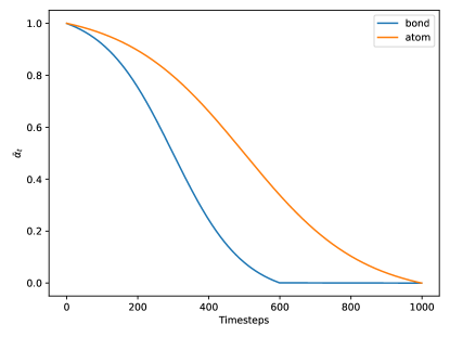
Figure 5: Noise schedule of atom and bond types.

B.3 Training Details

Pre-training

We use Adam [19] for pre-training, with init_learning_rate=0.0004 and betas=(0.95,0.999). The learning rate is scheduled to decay exponentially with a factor of 0.6 with minimize_learning_rate=1e-6. The learning rate is decayed if there is no improvement for the validation loss in 10 consecutive evaluations. We set batch_size=8 and clip_gradient_norm=8. During training, a small Gaussian noise with a standard deviation of 0.1 to protein atom positions is added as data augmentation. To balance the magnitude of different losses, the reconstruction losses of atom and bond type are multiplied with weights $\gamma_{v}=100$ and $\gamma_{b}=100$, separately. We perform evaluations for every 2000 training steps. The model is pre-trained on one NVIDIA GeForce RTX A6000 GPU, and it could converge within 21 hours and 170k steps.

Fine-tuning and Optimizing

For both fine-tuning and optimizing model with DecompDpo, we use the Adam optimizer with init_learning_rate=1e-6 and betas=(0.95,0.999). We maintain a constant learning rate throughout both processes. We set batch_size=4 and clip_gradient_norm=8. Consistent with pre-training, Gaussian noise is added to protein atom positions, and we use a weighted reconstruction loss. For fine-tuning model for molecule generation, we set $\beta_{T}=0.01$ and conduct training for 1 epoch across all preference pairs constructed from training set. In optimizing model for molecular optimization, we set $\beta_{T}=0.02$ and trained for 20,000 steps. We trained our model on one NVIDIA GeForce GTX V100 GPU and evaluate every 1,000 steps.

B.4 Experiment Details

The scoring function for selecting training molecules is defined as $S=w_{\text{QED}}\cdot QED+w_{\text{SA}}\cdot SA+w_{\text{Vina}}\cdot Vina\_Min/(-12)$, with each property weight set to 1. Vina Minimize Score is divided by -12 to ensure that it is generally ranges between 0 and 1. For molecule generation, we exclude molecules that cannot be decomposed or reconstructed, resulting in a total of 63,092 preference pairs available for fine-tuning. In molecular optimization, to ensure that the model maintains a desirable completion rate, we include an additional 50 molecules that failed in reconstruction in the preference pairs as the losing side. To tailor the optimization to a specific protein, the weights of the optimization objectives are defined as $w_{x}=e^{-(x-x_{s})}$, where $x$ is the mean property of the generated molecules and $x_{s}$ is the threshold of the property used in Success Rate. For both molecular optimization and evaluation, we employ the Opt Prior used in DecompDiff. Since binding affinity is mainly defined by the positions and types of atoms, we do not consider model’s log probabilities from bonds when aligning binding affinity related preferences.

To directly evaluate the improvements provided by DecompDpo, we have disabled the validity guidance used in DecompDiff sampling, which allows us to directly evaluate the improvement brought by DecompDpo. For both fine-tuning and optimization, we select the best checkpoint using 20 molecules with three key metrics: (success rate, completion rate, and $S$).

Appendix C Additional Results

C.1 Full Evaluation Results

Molecular Conformation

We provide a more comprehensive evaluation of the molecular conformation. We compute the Jensen-Shannon Divergence (JSD) of distances for different types of bonds between molecules from generative models and reference molecules. The detailed results are shown in Table 4, which demonstrates the reasonableness of our generated molecular structures.

Table 4: Jensen-Shannon Divergence of the bond distance distribution between the generated molecules and the reference molecule by bond type, with a lower value indicating better. “-”, “=”, and “:” represent single, double, and aromatic bonds, respectively. The top 2 results are highlighted with bold text and underlined text.

Bond liGAN GraphBP AR Pocket2Mol TargetDiff DecompDiff DecompDpo C$-$C 0.601 0.368 0.609 0.496 0.369 0.359 0.437 C$=$C 0.665 0.530 0.620 0.561 0.505 0.537 0.546 C$-$N 0.634 0.456 0.474 0.416 0.363 0.344 0.363 C$=$N 0.749 0.693 0.635 0.629 0.550 0.584 0.576 C$-$O 0.656 0.467 0.492 0.454 0.421 0.376 0.399 C$=$O 0.661 0.471 0.558 0.516 0.461 0.374 0.361 C$:$C 0.497 0.407 0.451 0.416 0.263 0.251 0.316 C$:$N 0.638 0.689 0.552 0.487 0.235 0.269 0.286

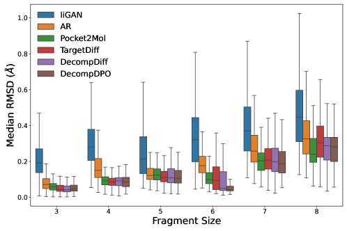
Figure 6: Median RMSD for rigid fragments of generated molecules before and after optimizing with the Merck Molecular Force Field

We also evaluate median RMSD of rigid fragments from generated molecules before and after molecular conformations optimized with Merck Molecular Force Field, which is shown in Figure 6.

Molecular Properties

To provide a comprehensive evaluation, we have expanded our evaluation metrics beyond those discussed in Section 4, which focused primarily on molecular properties and binding affinities. To assess the model’s efficacy in designing novel and valid molecules, we calculate the following additional metrics, which are reported in Table 5:

• Complete Rate is the percentage of generated molecules that are connected and vaild, which is defined by RDKit.

• Novelty is defined as the ratio of generated molecules that are different from the reference ligand of the corresponding pocket in the test set.

• Similarity is the Tanimoto Similarity between generated molecules and the corresponding reference ligand.

• Uniqueness is the proportion of unique molecules among generated molecules.

Table 5: Summary of the models’ ability in designing novel and valid molecules. ($\uparrow$) / ($\downarrow$) denotes a larger / smaller number is better.

Methods Complete Rate ($\uparrow$) Novelty ($\uparrow$) Similarity ($\downarrow$) Uniqueness ($\uparrow$) Generate LiGAN 99.11% 100% 0.22 87.82% AR 92.95% 100% 0.24 100% Pocket2Mol 98.31% 100% 0.26 100% TargetDiff 90.36% 100% 0.30 99.63% DecompDiff* 72.82% 100% 0.27 99.58% DecompDpo 71.75% 100% 0.26 99.95% Optimize RGA - 100% 0.37 96.82% DecompOpt 71.55% 100% 0.36 100% DecompDpo 65.05% 100% 0.26 99.63%

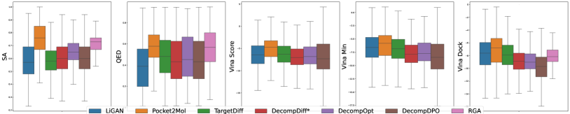
Figure 7: Boxplots of QED, SA, Vina Score, Vina Minimize, and Vina Dock of molecules generated by DecompDpo and all generative and optimization baselines.

We also draw boxplots to provide confidence intervals for our results, which is shown in Figure 7.

C.2 Effect of reference model in Molecular Optimization

Table 6: Ablation study of reference model in DecompDpo for molecular optimization. ($\uparrow$) / ($\downarrow$) denotes a larger / smaller number is better.

Method Vina Score ($\downarrow$) Vina Min ($\downarrow$) Vina Dock ($\downarrow$) High Affinity ($\uparrow$) QED ($\uparrow$) SA ($\uparrow$) Diversity ($\uparrow$) Success Avg. Med. Avg. Med. Avg. Med. Avg. Med. Avg. Med. Avg. Med. Avg. Med. Rate ($\uparrow$) DecompDpo -2.83 -7.33 -7.23 -8.45 -9.89 -9.69 85.6% 100.0% 0.48 0.46 0.63 0.64 0.61 0.62 54.9% DecompDpo (DecompDiff* as ref. model) -3.94 -7.88 -7.91 -8.84 -9.89 -9.86 88.2% 100.0% 0.48 0.47 0.62 0.64 0.61 0.62 54.0%

To assess the influence of the reference model on the performance of the DecompDpo, we performed an ablation study using DecopmDiff* as the reference model in molecular optimization. The results shown in Table 6 indicate that the performance when using DecopmDiff* is generally comparable to that achieved using a model fine-tuned with DecompDpo, which has a stronger capability in molecule generation. This finding suggests that the capability of the reference model does not limit the performance of DecompDpo in molecular optimization. It also implies that DecompDpo has reached an optimal level of performance with the given preference pairs.

C.3 Evidence for Decomposability of Properties

As illustrated in Section 3.2, since QED and SA are non-decomposable, we construct molecule-level preference for their optimization. As shown in Figure 8, the Person correlation coefficients between the property of molecules and summation from the corresponding structure do not exceed 0.1. Besides, a large proportion of the summed substructures’ properties are greater than 1, which is unreasonable for QED and SA.

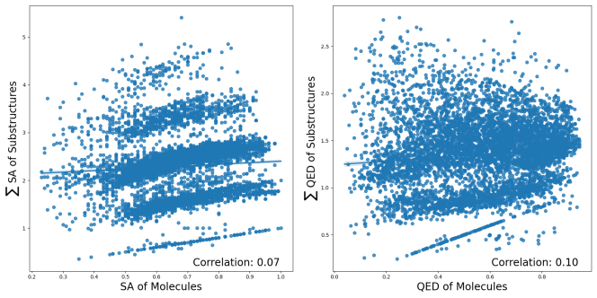
Figure 8: Person correlation coefficients between SA (left)/ QED(right) of molecules and summation from its corresponding substructures.

C.4 Trade-off in Multi-objective Optimization

As we select multiple optimization objectives with DecompDpo, inherent trade-offs between different properties are unavoidable. As illustrated in Figure 9, while molecules generated by DecompDpo exhibit significantly improved properties compared to those generated by DecompDiff, DecompDpo encounters a notable trade-off between optimizing the Vina Minimize Score and the SA.

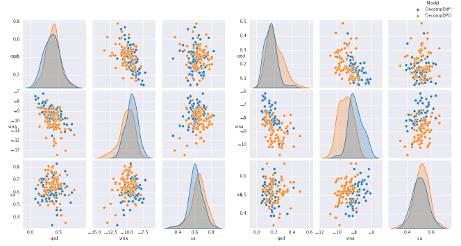
Figure 9: Pairplots of the molecular properties before and after optimization with DecompDpo. The left and right figure displays properties attained from molecules generated on protein 4Z2G and 2HCJ, separately.

C.5 Example of Generated Molecules

We provides more examples of molecules generated by DecompDpo, which are shown in Figure 10.

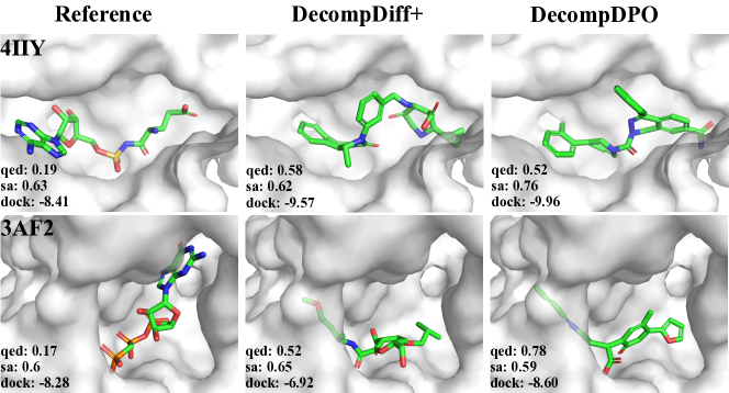
Figure 10: Additional Examples of reference binding ligands and the molecule with the highest property among all generated molecules of DecompDiff* and DecompDpo on protein 4IIY and 3AF2.

References

- Achiam et al. [2023] Josh Achiam, Steven Adler, Sandhini Agarwal, Lama Ahmad, Ilge Akkaya, Florencia Leoni Aleman, Diogo Almeida, Janko Altenschmidt, Sam Altman, Shyamal Anadkat, et al. 2023. Gpt-4 technical report. arXiv preprint arXiv:2303.08774.
- Anderson [2003] Amy C Anderson. 2003. The process of structure-based drug design. Chemistry & biology, 10(9):787–797.
- Bai et al. [2022] Yuntao Bai, Saurav Kadavath, Sandipan Kundu, Amanda Askell, Jackson Kernion, Andy Jones, Anna Chen, Anna Goldie, Azalia Mirhoseini, Cameron McKinnon, et al. 2022. Constitutional ai: Harmlessness from ai feedback. arXiv preprint arXiv:2212.08073.
- Bickerton et al. [2012] G Richard Bickerton, Gaia V Paolini, Jérémy Besnard, Sorel Muresan, and Andrew L Hopkins. 2012. Quantifying the chemical beauty of drugs. Nature chemistry, 4(2):90–98.
- Black et al. [2023] Kevin Black, Michael Janner, Yilun Du, Ilya Kostrikov, and Sergey Levine. 2023. Training diffusion models with reinforcement learning. arXiv preprint arXiv:2305.13301.
- Christiano et al. [2017] Paul F Christiano, Jan Leike, Tom Brown, Miljan Martic, Shane Legg, and Dario Amodei. 2017. Deep reinforcement learning from human preferences. Advances in neural information processing systems, 30.
- Eberhardt et al. [2021] Jerome Eberhardt, Diogo Santos-Martins, Andreas F Tillack, and Stefano Forli. 2021. AutoDock Vina 1.2. 0: New docking methods, expanded force field, and python bindings. Journal of chemical information and modeling, 61(8):3891–3898.
- Ertl and Schuffenhauer [2009] Peter Ertl and Ansgar Schuffenhauer. 2009. Estimation of synthetic accessibility score of drug-like molecules based on molecular complexity and fragment contributions. Journal of cheminformatics, 1(1):1–11.
- Fan et al. [2024] Ying Fan, Olivia Watkins, Yuqing Du, Hao Liu, Moonkyung Ryu, Craig Boutilier, Pieter Abbeel, Mohammad Ghavamzadeh, Kangwook Lee, and Kimin Lee. 2024. Reinforcement learning for fine-tuning text-to-image diffusion models. Advances in Neural Information Processing Systems, 36.
- Francoeur et al. [2020] Paul G Francoeur, Tomohide Masuda, Jocelyn Sunseri, Andrew Jia, Richard B Iovanisci, Ian Snyder, and David R Koes. 2020. Three-dimensional convolutional neural networks and a cross-docked data set for structure-based drug design. Journal of chemical information and modeling, 60(9):4200–4215.
- Fu et al. [2022] Tianfan Fu, Wenhao Gao, Connor Coley, and Jimeng Sun. 2022. Reinforced genetic algorithm for structure-based drug design. Advances in Neural Information Processing Systems, 35:12325–12338.
- Guan et al. [2023a] Jiaqi Guan, Wesley Wei Qian, Xingang Peng, Yufeng Su, Jian Peng, and Jianzhu Ma. 2023a. 3D Equivariant Diffusion for Target-Aware Molecule Generation and Affinity Prediction. In International Conference on Learning Representations.
- Guan et al. [2023b] Jiaqi Guan, Xiangxin Zhou, Yuwei Yang, Yu Bao, Jian Peng, Jianzhu Ma, Qiang Liu, Liang Wang, and Quanquan Gu. 2023b. DecompDiff: Diffusion Models with Decomposed Priors for Structure-Based Drug Design. In Proceedings of the 40th International Conference on Machine Learning, volume 202 of Proceedings of Machine Learning Research, pages 11827–11846. PMLR.
- Halgren [1996] Thomas A Halgren. 1996. Merck molecular force field. I. Basis, form, scope, parameterization, and performance of MMFF94. Journal of computational chemistry, 17(5-6):490–519.
- Harris et al. [2023] Charles Harris, Kieran Didi, Arian R Jamasb, Chaitanya K Joshi, Simon V Mathis, Pietro Lio, and Tom Blundell. 2023. Benchmarking Generated Poses: How Rational is Structure-based Drug Design with Generative Models? arXiv preprint arXiv:2308.07413.
- Ho et al. [2020] Jonathan Ho, Ajay Jain, and Pieter Abbeel. 2020. Denoising diffusion probabilistic models. Advances in neural information processing systems, 33:6840–6851.
- Huang et al. [2023] Zhilin Huang, Ling Yang, Xiangxin Zhou, Zhilong Zhang, Wentao Zhang, Xiawu Zheng, Jie Chen, Yu Wang, CUI Bin, and Wenming Yang. 2023. Protein-ligand interaction prior for binding-aware 3d molecule diffusion models. In The Twelfth International Conference on Learning Representations.
- Jin et al. [2020] Wengong Jin, Regina Barzilay, and Tommi Jaakkola. 2020. Multi-objective molecule generation using interpretable substructures. In International conference on machine learning, pages 4849–4859. PMLR.
- Kingma and Ba [2014] Diederik P Kingma and Jimmy Ba. 2014. Adam: A method for stochastic optimization. arXiv preprint arXiv:1412.6980.
- Lee et al. [2023] Harrison Lee, Samrat Phatale, Hassan Mansoor, Kellie Lu, Thomas Mesnard, Colton Bishop, Victor Carbune, and Abhinav Rastogi. 2023. Rlaif: Scaling reinforcement learning from human feedback with ai feedback. arXiv preprint arXiv:2309.00267.
- Lin et al. [2022] Haitao Lin, Yufei Huang, Meng Liu, Xuanjing Li, Shuiwang Ji, and Stan Z Li. 2022. Diffbp: Generative diffusion of 3d molecules for target protein binding. arXiv preprint arXiv:2211.11214.
- Liu et al. [2022] Meng Liu, Youzhi Luo, Kanji Uchino, Koji Maruhashi, and Shuiwang Ji. 2022. Generating 3d molecules for target protein binding. arXiv preprint arXiv:2204.09410.
- Luo et al. [2021] Shitong Luo, Jiaqi Guan, Jianzhu Ma, and Jian Peng. 2021. A 3D generative model for structure-based drug design. Advances in Neural Information Processing Systems, 34:6229–6239.
- Ouyang et al. [2022] Long Ouyang, Jeffrey Wu, Xu Jiang, Diogo Almeida, Carroll Wainwright, Pamela Mishkin, Chong Zhang, Sandhini Agarwal, Katarina Slama, Alex Ray, et al. 2022. Training language models to follow instructions with human feedback. Advances in neural information processing systems, 35:27730–27744.
- Peng et al. [2023] Xingang Peng, Jiaqi Guan, Qiang Liu, and Jianzhu Ma. 2023. MolDiff: addressing the atom-bond inconsistency problem in 3D molecule diffusion generation. arXiv preprint arXiv:2305.07508.
- Peng et al. [2022] Xingang Peng, Shitong Luo, Jiaqi Guan, Qi Xie, Jian Peng, and Jianzhu Ma. 2022. Pocket2mol: Efficient molecular sampling based on 3d protein pockets. In International Conference on Machine Learning, pages 17644–17655. PMLR.
- Powers et al. [2023] Alexander S Powers, Helen H Yu, Patricia Suriana, Rohan V Koodli, Tianyu Lu, Joseph M Paggi, and Ron O Dror. 2023. Geometric deep learning for structure-based ligand design. ACS Central Science, 9(12):2257–2267.
- Rafailov et al. [2024] Rafael Rafailov, Archit Sharma, Eric Mitchell, Christopher D Manning, Stefano Ermon, and Chelsea Finn. 2024. Direct preference optimization: Your language model is secretly a reward model. Advances in Neural Information Processing Systems, 36.
- Ragoza et al. [2022] Matthew Ragoza, Tomohide Masuda, and David Ryan Koes. 2022. Generating 3D molecules conditional on receptor binding sites with deep generative models. Chemical science, 13(9):2701–2713.
- Schneuing et al. [2022] Arne Schneuing, Yuanqi Du, Charles Harris, Arian Jamasb, Ilia Igashov, Weitao Du, Tom Blundell, Pietro Lió, Carla Gomes, Max Welling, Michael Bronstein, and Bruno Correia. 2022. Structure-based Drug Design with Equivariant Diffusion Models. arXiv preprint arXiv:2210.13695.
- Schulman et al. [2017] John Schulman, Filip Wolski, Prafulla Dhariwal, Alec Radford, and Oleg Klimov. 2017. Proximal policy optimization algorithms. arXiv preprint arXiv:1707.06347.
- Spiegel and Durrant [2020] Jacob O Spiegel and Jacob D Durrant. 2020. AutoGrow4: an open-source genetic algorithm for de novo drug design and lead optimization. Journal of cheminformatics, 12(1):1–16.
- Stiennon et al. [2020] Nisan Stiennon, Long Ouyang, Jeffrey Wu, Daniel Ziegler, Ryan Lowe, Chelsea Voss, Alec Radford, Dario Amodei, and Paul F Christiano. 2020. Learning to summarize with human feedback. Advances in Neural Information Processing Systems, 33:3008–3021.
- Touvron et al. [2023] Hugo Touvron, Thibaut Lavril, Gautier Izacard, Xavier Martinet, Marie-Anne Lachaux, Timothée Lacroix, Baptiste Rozière, Naman Goyal, Eric Hambro, Faisal Azhar, et al. 2023. Llama: Open and efficient foundation language models. arXiv preprint arXiv:2302.13971.
- Vamathevan et al. [2019] Jessica Vamathevan, Dominic Clark, Paul Czodrowski, Ian Dunham, Edgardo Ferran, George Lee, Bin Li, Anant Madabhushi, Parantu Shah, Michaela Spitzer, et al. 2019. Applications of machine learning in drug discovery and development. Nature reviews Drug discovery, 18(6):463–477.
- Wallace et al. [2023] Bram Wallace, Meihua Dang, Rafael Rafailov, Linqi Zhou, Aaron Lou, Senthil Purushwalkam, Stefano Ermon, Caiming Xiong, Shafiq Joty, and Nikhil Naik. 2023. Diffusion model alignment using direct preference optimization. arXiv preprint arXiv:2311.12908.
- Xie et al. [2021] Yutong Xie, Chence Shi, Hao Zhou, Yuwei Yang, Weinan Zhang, Yong Yu, and Lei Li. 2021. {MARS}: Markov Molecular Sampling for Multi-objective Drug Discovery. In International Conference on Learning Representations.
- Zhang et al. [2024] Yinan Zhang, Eric Tzeng, Yilun Du, and Dmitry Kislyuk. 2024. Large-scale Reinforcement Learning for Diffusion Models. arXiv preprint arXiv:2401.12244.
- Zhang and Liu [2023] Zaixi Zhang and Qi Liu. 2023. Learning Subpocket Prototypes for Generalizable Structure-based Drug Design. arXiv preprint arXiv:2305.13997.
- Zhang et al. [2022] Zaixi Zhang, Yaosen Min, Shuxin Zheng, and Qi Liu. 2022. Molecule generation for target protein binding with structural motifs. In The Eleventh International Conference on Learning Representations.
- Zhou et al. [2024a] Xiangxin Zhou, Xiwei Cheng, Yuwei Yang, Yu Bao, Liang Wang, and Quanquan Gu. 2024a. DecompOpt: Controllable and Decomposed Diffusion Models for Structure-based Molecular Optimization. In The Twelfth International Conference on Learning Representations.
- Zhou et al. [2024b] Xiangxin Zhou, Dongyu Xue, Ruizhe Chen, Zaixiang Zheng, Liang Wang, and Quanquan Gu. 2024b. Antigen-Specific Antibody Design via Direct Energy-based Preference Optimization. arXiv preprint arXiv:2403.16576.
- Ziegler et al. [2019] Daniel M Ziegler, Nisan Stiennon, Jeffrey Wu, Tom B Brown, Alec Radford, Dario Amodei, Paul Christiano, and Geoffrey Irving. 2019. Fine-tuning language models from human preferences. arXiv preprint arXiv:1909.08593.