Byzantine-tolerant distributed learning of finite mixture models

Abstract

This paper proposes two split-and-conquer (SC) learning estimators for finite mixture models that are tolerant to Byzantine failures. In SC learning, individual machines obtain local estimates, which are then transmitted to a central server for aggregation. During this communication, the server may receive malicious or incorrect information from some local machines, a scenario known as Byzantine failures. While SC learning approaches have been devised to mitigate Byzantine failures in statistical models with Euclidean parameters, developing Byzantine-tolerant methods for finite mixture models with non-Euclidean parameters requires a distinct strategy. Our proposed distance-based methods are hyperparameter tuning free, unlike existing methods, and are resilient to Byzantine failures while achieving high statistical efficiency. We validate the effectiveness of our methods both theoretically and empirically via experiments on simulated and real data from machine learning applications for digit recognition. The code for the experiment can be found at https://github.com/SarahQiong/RobustSCGMM.

Keywords: Aggregation, Byzantine failure, distributed inference, finite mixture model, robustness.

1 Introduction

Mixture models can effectively represent data originating from populations with latent homogeneous subpopulations. The roots of this model trace back to the pioneering work of Pearson (1894), who applied it to infer the existence of subspecies in crabs. Over the years, these models have demonstrated their versatility across diverse fields such as finance (Liesenfeld, 2001), astronomy (Baldry et al., 2004), image analysis (Salimans et al., 2016). Their impact also extends into medical realms, contributing to modeling of patient lifespans with lupus nephritis (Marín et al., 2005), refined delineation of breast cancer tumor stages (Fraley and Raftery, 2002), and identifying post-stem cell transplantation states (Baudry et al., 2010).

Mixture models have encountered new challenges in the era of big data, particularly in scaling inference methods to accommodate modern large-scale datasets (Nowak, 2003; Gu, 2008; Liu and Ihler, 2014; Ge et al., 2015; Lucic et al., 2017; Zhang and Chen, 2022; Tian et al., 2024). With data sizes often exceeding the capacity of a single device in real-world applications, a paradigm of distributed storage across multiple machines has emerged. The Split-and-Conquer (SC) learning techniques have been developed to effectively handle large datasets, particularly when they are stored in a distributed manner. SC procedures tackle the challenge of big data by first independently learning on local machines, followed by aggregating locally learned estimates on a central server. Numerous SC procedures have been developed in various applications in recent years (Li et al., 2013; Chen and Xie, 2014; Zhang et al., 2015; Chang et al., 2017; Lee et al., 2017; Battey et al., 2018; Fan et al., 2019; Jordan et al., 2019; Chen et al., 2022; Fan et al., 2023; Wu et al., 2023). These approaches typically address models with Euclidean parameter spaces and employ linear averaging to combine local estimates.

While aggregating locally learned parameter values via averaging is effective for models with Euclidean parameters, it presents challenges for finite mixture models. Local estimates under finite mixture models are discrete distributions with a fixed number of support points. Averaging these estimates often yields values outside the parameter space, leading to impractical outcomes. Therefore, learning finite mixtures via SC necessitates specialized techniques, as proposed by Zhang and Chen (2022), which identify the mixing distribution in the parameter space closest to the averaged mixture using specific divergence measures.

The SC framework, while effective for large-scale inference, can be susceptible to Byzantine failure (Lamport et al., 1982). In real-world applications, issues such as hardware or software malfunctions, data corruption, or communication disruptions can introduce inaccuracies during information transmission from local machines. Specifically, a subset of these machines, known as Byzantine machines, may transmit arbitrary or malicious messages to the server, thereby leading to deteriorated aggregation results. In the presence of Byzantine failure, each transmitted local estimate may either match the authentic local estimate or be altered in an unknown manner. To address the risk posed by Byzantine failures, numerous Byzantine failure-tolerant strategies have been developed and explored in recent years (Chen et al., 2017; Alistarh et al., 2018; Xie et al., 2018; Yin et al., 2018; Minsker, 2019; Yin et al., 2019; Tu et al., 2021; Wang et al., 2024). For instance, Yin et al. (2018) and Yin et al. (2019) consider the trimmed mean, Chen et al. (2017) and Feng et al. (2015) consider the geometric median, Xie et al. (2018) considers the mean around median,  Tu et al. (2021) considers a variance reduced median-of-means estimator. Wang et al. (2024) considers the distributed empirical likelihood inference under Byzantine failure. However, these strategies are primarily tailored for models with Euclidean parameters and cannot be directly applied to the non-Euclidean parameter space of mixture model. Moreover, there is no straightforward generalization of median or trimmed mean in mixture model’s paramater space.

To the best of our knowledge, there is no existing work specifically addressing the issue of Byzantine failure in the SC learning of finite mixtures. One relevant work is robust clustering of non-Euclidean objects by Del Barrio et al. (2019). Inspired by the $k$-means algorithm, Del Barrio et al. (2019) iteratively partitions objects into $k$ groups, each centered around a barycenter. To ensure robustness against outliers, they introduce trimmed $k$ barycenters, which temporarily exclude a proportion of objects furthest from their closest cluster centers during each iteration. While their approach can be applied for Byzantine failure tolerant distributed learning of non-Euclidean mixing distributions, it relies on a predetermined trimming level, posing challenges in Byzantine failure scenarios. Moreover, their method is also ineffective at addressing outliers in mixing weights. Tian et al. (2024) study the theoretical properties of the distributed Expectation-Maximization (EM) algorithm for learning finite mixture models. Their framework considers scenarios where a small fraction of machines may contain outliers or be vulnerable to adversarial attacks, while the remaining machines possess random samples from similar but not identical mixtures. Their goal is to construct a representative finite mixture model using a distributed one-step gradient EM algorithm. This involves an iterative process where local EM updates are sent to the central machine for aggregation, which then solves a penalized least squares problem to encourage consensus aggregation. The aggregated value is then sent back to local machines for the next round of updates. Despite demonstrated resilience against a limited proportion (less than $1/3$) of Byzantine failures, their approach incurs significant computational overhead due to multiple rounds of communication between central and local machines.

This paper proposes Byzantine failure-tolerant aggregation strategies specifically designed for finite mixture models. Existing methods for Byzantine-tolerant aggregation share the common principle of discarding unreliable local estimates suspected of Byzantine failure, albeit differing in the extent of discarding. Our approach follows the same principle by either keeping reliable local estimates or discarding those likely affected by Byzantine failures. Consider the scenario where the majority of transmitted local estimates are of high quality, with only a minority experiencing failures. In this case, the quality estimates cluster closely together. Conversely, estimates affected by Byzantine failures scatter widely. We introduce a distance-based procedure to identify the region containing the most failure-free estimates. Aggregating these identified failure-free local estimates leads to Byzantine failure-tolerant yet highly efficient SC learning methods. Notably, our approach does not require a pre-specified trimming level unlike Del Barrio et al. (2019), and is purely data-dependent. We prove that our proposed method consistently detects the failure machines under some general conditions.

The paper is structured as follows. In Section 2, we introduce finite mixture models and the concept of Byzantine failure. Section 3 presents two Byzantine-tolerant aggregation approaches. Their statistical properties are described in Section 4. We then conduct numerical experiments on simulated datasets in Section 5 and on real data in Section 6 to illustrate the effectiveness of the proposed method. Finally, Section 7 offers discussion and concluding remarks.

2 Preliminaries

This section introduces the concepts of finite mixture models, outlines the general procedure for their split-and-conquer learning. Additionally, we formally define the problem of Byzantine failure in the context of distributed learning of finite mixtures.

2.1 SC learning of finite mixture without Byzantine failure

A finite mixture model is a special family of distributions defined formally as follows:

Definition 2.1 (Finite mixture model).

Let ${\mathcal{F}}=\{f(x;\theta):x\in{\mathcal{X}}\subseteq{\mathbb{R}}^{d},\theta\in\Theta\subseteq{\mathbb{R}}^{p}\}$ be density functions representing a classical parametric model, where $d$ and $p$ denote the dimensions of the observation and parameter space respectively. An order $K$ finite mixture of ${\mathcal{F}}$ consists of distributions, each having a density function given by:

$$f_{G}(x):=\int_{\Theta}f(x;\theta)\,dG(\theta)=\sum_{k=1}^{K}w_{k}f(x;\theta_{k})$$

where the parameter $G=\sum_{k=1}^{K}w_{k}\delta_{\theta_{k}}$, called the mixing distribution, assigns probability $w_{k}$ to $\theta_{k}$, $k\in[K]$. Here, $f(x;\theta_{k})$ represents subpopulation densities, $\theta_{k}\in\Theta$ are subpopulation or component parameters, and $w_{k}\geq 0$ are mixing weights satisfying $\sum_{k=1}^{K}w_{k}=1$. We denote ${\mathbb{G}}_{K}$ as the family of mixing distributions with at most $K$ distinct support points.

Alternatively, one may propose to parameterize the finite mixture model using a vector such as $(w_{1},w_{2},\ldots,w_{K},\theta_{1},\theta_{2},\ldots,\theta_{K})^{\top}$ instead of the mixing distribution $G$. However, this choice suffers from the well-known label switching dilemma, where permutations of the parameters (e.g., $(w_{K},w_{K-1},\ldots,w_{1},\theta_{K},\theta_{K-1},\ldots,\theta_{1})^{\top}$ and $K!$ of such permutations in total) lead to the same mixture distribution. Parameterizing by $G$ effectively mitigates this dilemma but still precludes the use of traditional aggregation methods in Euclidean parameter space, as detailed below.

Let ${\mathcal{X}}=\{x_{ij}:i\in[m],j\in[n_{i}]\}$ be $N=\sum_{i}n_{i}$ independently and identically distributed (IID) samples from a mixture distribution $f_{G^{*}}(x)$ for some $G^{*}\in{\mathbb{G}}_{K}$. Suppose ${\mathcal{X}}$ is randomly partitioned into $m$ subsets ${\mathcal{X}}_{1},\ldots,{\mathcal{X}}_{m}$, which are stored in a distributed manner on $m$ local machines, where ${\mathcal{X}}_{i}=\{x_{ij}:j\in[n_{i}]\}$ for $i\in[m]$. A general SC procedure for learning a finite mixture consists of the following two steps:

• Local inference: Obtain the local estimator $\widehat{G}_{i}=\sum_{k}\hat{w}_{ik}\delta_{\hat{\theta}_{ik}}$ by maximizing the log-likelihood function $\ell_{i}(G)=\sum_{j=1}^{n_{i}}\log f_{G}(x_{ij})$ or its penalized version in the case of Gaussian mixture (Chen and Tan, 2009), based on the data $\mathcal{X}_{i}$ on the $i$th machine. These local estimators are referred to as referred to as Maximum Likelihood Estimates (MLE) or penalized MLEs (pMLE) respectively. EM algorithms can be used for numerical computation of MLE or pMLE, see Appendix A.1.

• Global aggregation: Send $\{\widehat{G}_{i}:i\in[m]\}$ to a server and aggregate them to produce final estimator $\widehat{G}$. The final estimator is

  $$\widehat{G}_{{\mathcal{I}}}^{\mathfrak{A}}=\mathfrak{A}(\{\widehat{G}_{i}:i\in{\mathcal{I}}\subset[m]\}),$$ (1)

  where $\mathfrak{A}(\cdot)$ is some aggregation operator such as the one in Zhang and Chen (2022) and ${\mathcal{I}}=[m]$ when there are no Byzantine failures.

For completeness, we provide a concise overview of the aggregation approach in Zhang and Chen (2022). Recall that $\{\widehat{G}_{i}=\sum_{k}\hat{w}_{ik}\delta_{\hat{\theta}_{ik}}:i\in[m]\}$ represent the local estimates of the mixing distribution $G^{*}$, which are to be aggregated. Let the average mixing distribution be

$$\macc@depth\char 1\relax\frozen@everymath{\macc@group}\macc@set@skewchar\macc@nested@a 111{G}_{m}=\sum_{i=1}^{m}\lambda_{i}\widehat{G}_{i}$$

where $\lambda_{i}=n_{i}/N$ is the proportion of data stored on $i$th machine. Since each $\widehat{G}_{i}$ is a probability measure and is close to the true mixing distribution $G^{*}$, $\macc@depth\char 1\relax\frozen@everymath{\macc@group}\macc@set@skewchar\macc@nested@a 111{G}_{m}$ is also close to $G^{*}$. However, it is most likely that $\macc@depth\char 1\relax\frozen@everymath{\macc@group}\macc@set@skewchar\macc@nested@a 111{G}_{m}\in{\mathbb{G}}_{Km}$ rather than ${\mathbb{G}}_{K}$, even though $\widehat{G}_{i}\in{\mathbb{G}}_{K}$ for all $i$. Therefore, aggregation via simple averaging is not appropriate under finite mixture models. To address this issue, one may seek a mixing distribution $G\in{\mathbb{G}}_{K}$ that is closest to $\macc@depth\char 1\relax\frozen@everymath{\macc@group}\macc@set@skewchar\macc@nested@a 111{G}_{m}$. This task can be framed as approximating a high-order mixture using a lower-order mixture. The resulting solution is commonly referred to as a reduction estimator (Crouse et al., 2011). In the context of Gaussian mixtures, this process is known as Gaussian Mixture Reduction (GMR).

A GMR for SC aggregation necessitates both statistical and computational efficiency. To achieve this, Zhang and Chen (2022) use an efficient Majorization-Minimization (MM) algorithm to minimize a composite transportation divergence to $\macc@depth\char 1\relax\frozen@everymath{\macc@group}\macc@set@skewchar\macc@nested@a 111{G}_{m}$. Specifically, let $c:{\mathcal{F}}\times{\mathcal{F}}\to{\mathbb{R}}_{+}$ be a cost function, where $c(\theta,\theta^{\prime})=c(f(\cdot;\theta),f(\cdot;\theta^{\prime}))$ for simplicity. Let

$$G=\sum_{i=1}^{m}\pi_{i}\delta_{\theta_{i}}\quad\text{and}\quad G^{\prime}=\sum_{j=1}^{n}\pi^{\prime}_{j}\delta_{\theta^{\prime}_{j}}$$

be two mixing distributions with $m$ and $n$ support points. The composite transportation divergence between these mixing distributions is defined to be

$$T_{c}(G,G^{\prime})=\inf\Big{\{}\sum_{i,j}\pi_{i,j}c(\theta_{i},\theta^{\prime}_{j}):~{}\sum_{i}\pi_{ij}=\pi^{\prime}_{j},\sum_{j}\pi_{ij}=\pi_{i},\pi_{ij}\geq 0\Big{\}}.$$

This divergence is the lowest cost of transporting subpopulations of $G$ to those of $G^{\prime}$ (Chen et al., 2019; Delon and Desolneux, 2020). The reduction estimator is then defined to be

$$\widehat{G}^{\text{GMR}}=\operatorname*{arg\,min}_{G\in{\mathbb{G}}_{K}}T_{c}(\macc@depth\char 1\relax\frozen@everymath{\macc@group}\macc@set@skewchar\macc@nested@a 111{G}_{m},G).$$ (2)

An iterative MM algorithm can be used to compute $\widehat{G}^{\text{GMR}}$, see concrete steps in Appendix A.2.

2.2 Byzantine failure

The Byzantine failure is a well-recognized challenge in distributed learningr (Lamport et al., 1982), occurring when a subset of local machines within the system transmits erroneous or even malicious data to the central server. Such errors can stem from various sources, including hardware or software glitches, data corruption, or communication interruptions. If any machine suffer unnoticed Byzantine failure, the aggregated estimate $\widehat{G}_{[m]}^{\mathfrak{A}}$ in (1) becomes unreliable or irrelevant.

Let $\widehat{G}_{j}$ and $\widetilde{G}_{j}$ respectivley be the local and transmitted estimates of the $j$th local machine. A subset ${\mathbb{B}}^{*}\subset[m]$ of local machines suffer from Byzantine failure if

$$\widetilde{G}_{j}=\begin{cases}\widehat{G}_{j},&\text{ when }j\notin{\mathbb{B}}^{*}\\ *,&\text{ when }j\in{\mathbb{B}}^{*}\end{cases}$$

where $*$ represents an arbitrary mixing distribution, potentially contaminated, seriously distorted, or entirely fake. We focus on scenarios where more than half of the local estimates were transmitted error-free. Although one might consider situations where some aspects of $\widehat{G}_{j}$ are preserved for some $j\in{\mathbb{B}}^{*}$, this is not the primary focus of this paper, and we leave it for future work.

Our objective is to aggregate the transmitted local estimates $\widetilde{{\mathcal{G}}}=\{\widetilde{G}_{j}:j\in[m]\}$ to arrive at a final $\widehat{G}$, ensuring both statistical reliability and computational efficiency. If ${\mathbb{B}}^{*}$ is known, we may discard the erroneous local estimates and aggregate the remaining error-free local estimates via $\mathfrak{A}(\{\widetilde{G}_{j}:j\not\in{\mathbb{B}}^{*}\})$ as the final estimate. Otherwise, a robust aggregation may involve first identifying local estimates that suffered from Byzantine failures as much as possible, followed by aggregating the remaining local estimates.

For models with Euclidean parameters, Byzantine failures are viewed as outliers, and classical robust methods such as the trimmed mean (Yin et al., 2018) and the median (Minsker, 2019) are often used to aggregate local estimators. However, due to the label switching dilemma mentioned earlier, neither elementwise trimmed mean nor median can be directly applied to mixture models. This limitation arises because the estimates for the $K$ subpopulations from different machines are not aligned, and aligning these subpopulation estimates under Byzantine failure may present additional challenges. Moreover, there is no straightforward generalization of the median or trimmed mean in the space of mixing distributions that can robustly aggregate the estimated mixing distributions. To address the risk of Byzantine failures in finite mixture models, we propose a novel approach as detailed in the following section.

3 Proposed Byzantine-tolerant SC methods

In most cases, the unaffected local estimates are within $o_{p}(1)$ distance from the true mixing distribution $G^{*}$. Conversely, affected local estimates scatter arbitrarily in ${\mathbb{G}}_{K}$. Consequently, the transmitted local estimates adhere to:

$$(\textbf{C1})\min_{i\not\in{\mathbb{B}}^{*},j\in{\mathbb{B}}^{*}}D(\widetilde{G}_{i},\widetilde{G}_{j})>\max_{i,j\not\in{\mathbb{B}}^{*}}D(\widetilde{G}_{i},\widetilde{G}_{j})$$

under any properly selected metric $D(\cdot,\cdot)$ on ${\mathbb{G}}_{K}$. We use this property to identify the subset ${\mathbb{B}}^{*}$ and aggregate the remaining local estimates to obtain an estimate with high statistical efficiency.

3.1 CRED estimator

Without prior knowledge of the subset of local machines suffering from Byzantine failures, we first identify a region in ${\mathbb{G}}_{K}$ centered at a local estimate that contains most failure-free estimates.

Figure 1: Three out of $m=10$ local machines are affected by Byzantine failure. Unaffected local estimates (blue dots) are clustered, while affected ones (red triangles) are scattered. The COAT (yellow star) and other $4$ local estimates that are closest to COAT are in the grey circle, and they are unaffected.

Let us introduce the integrated squared error (ISE):

$$D(G^{\prime},G)=D_{\text{ISE}}(G^{\prime},G)=\left\{\int\{f_{G^{\prime}}(x)-f_{G}(x)\}^{2}\,dx\right\}^{1/2},$$

as our default distance on ${\mathbb{G}}_{K}$ unless otherwise specified. ISE has a closed-form expression under most commonly employed finite mixtures. It enables efficient numerical evaluation compared to many other distances. We denote the open ball centered at $G$ with radius $r$ by

$$B_{D}(G;r)=\{G^{\prime}:D(G^{\prime},G)\leq r,G^{\prime}\in{\mathbb{G}}_{K}\}.$$

Given the set of transmitted local estimates $\widetilde{{\mathcal{G}}}=\{\widetilde{G}_{j}:j\in[m]\}$, let

$$r({G})=\min\left\{r:\mbox{Card}(\{G^{\prime}:G^{\prime}\in B_{D}(G;r)\cap\widetilde{{\mathcal{G}}}\})\geq(1/2)\mbox{Card}(\widetilde{{\mathcal{G}}})\right\}$$

be the shortest radius of the ball centered at $G$ so that $B_{D}(G;r(G))$ contains at least $50\%$ of local estimates. Following Nissim et al. (2007), we define the Center Of ATtention (COAT):

$$\widehat{G}^{\mbox{\tiny{COAT}}}=\arg\min_{G\in\widetilde{{\mathcal{G}}}}r(G).$$ (3)

It is important to note that Nissim et al. (2007) use COAT to obtain differentially private estimates under mixture models in a non-distributed learning setting, serving a different purpose.

Because every failure-free local estimate is satisfactory, we show in Theorem 4.1 that $\widehat{G}^{\mbox{\tiny{COAT}}}$ is also failure-free and thus Byzantine failure tolerant. Furthermore, let $r^{\mbox{\tiny{COAT}}}=r(\widehat{G}^{\mbox{\tiny{COAT}}})$ and

$$\widehat{{\mathbb{B}}}^{\mbox{\tiny{CRED}}}=\{j:~{}D(\widehat{G}^{\mbox{\tiny{COAT}}},\widetilde{G}_{j})\geq r^{\mbox{\tiny{COAT}}}\}.$$ (4)

We show in Theorem 4.1 that all $\{\widetilde{G}_{j}:j\not\in\widehat{{\mathbb{B}}}^{\mbox{\tiny{CRED}}}\}$ are Byzantine failure-free in probability. Hence, a more satisfactory Byzantine failure-tolerant estimator is the Coat REDuction (CRED) estimator defined as follows:

$$\widehat{G}^{\mbox{\tiny{CRED}}}=\mathfrak{A}(\{\widetilde{G}_{j}:j\not\in\widehat{{\mathbb{B}}}^{\mbox{\tiny{CRED}}}\}).$$

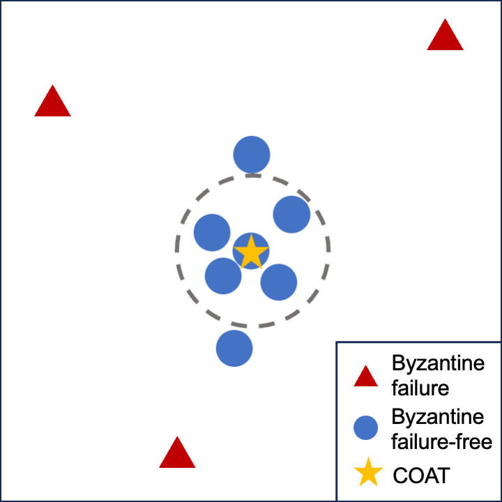
While any sensible aggregation operator $\mathfrak{A}(\cdot)$ could be used, we recommend the one from Zhang and Chen (2022) in (2) due to its computational and statistical efficiency. A cartoon example illustrating the idea of COAT and CRED is given in Figure 1.

3.2 ARED estimator

When the failure rate $\alpha$ is below 50%, $\widehat{G}^{\mbox{\tiny{CRED}}}$ has not yet leveraged all failure-free local estimates to obtain the final estimate. To further enhance efficiency, we propose an alternative approach based on asymptotic analysis, which does not require any hyper-parameter tuning.

Consider the scenario where the number of local machines $m=O(N^{\beta})$ for some $\beta\in[0,1)$, scaling with the total sample size $N$ so that $n=\min\{n_{j}\}$ goes to infinity at the order of $N^{1-\beta}$. We show that there is a considerable margin in $D(\widetilde{G}_{j},G^{*})$ to distinguish between $j\in{\mathbb{B}}^{*}$ and $j\not\in{\mathbb{B}}^{*}$, without the need for overly stringent mathematical bounds.

Recall that $\widehat{G}$ represents regular estimates, while $\widetilde{G}$ represents estimates that are potentially affected by Byzantine failures. As detailed in the following section, for each $j\in[m]$, we have $D(\widehat{G}_{j},G^{*})=O_{p}(n^{-1/2})=o_{p}(N^{-(1-\beta)/2})$. This rate holds in general when the order of the finite mixture model is known. In this case, $\{\widetilde{G}_{j}:j\not\in{\mathbb{B}}^{*}\}$ are within an $N^{-(1-\beta)/2}$ neighborhood of $G^{*}$ while $\{\widetilde{G}_{j}:j\in{\mathbb{B}}^{*}\}$ are significantly distant. This distinction makes it asymptotically simple to identify ${\mathbb{B}}^{*}$ as

$$\widehat{{\mathbb{B}}}^{\mbox{\tiny{ARED}}}=\left\{j:D(\widetilde{G}_{j},\widehat{G}^{\mbox{\tiny{COAT}}})>r^{\mbox{\tiny{COAT}}}\sqrt{\frac{1}{2}\log\left(\frac{m}{2}\right)\log\log m}\right\}.$$ (5)

Namely, if a transmitted local estimate’s distance from $\widehat{G}^{\mbox{\tiny{COAT}}}$ far exceeds $r^{\mbox{\tiny{COAT}}}$, it is labeled as suffering from Byzantine failure. The $\sqrt{(1/2)\log(m/2)\log\log m}$ factor is introduced to ensure consistency. It is of proper size for all the cases in simulations. Our Adaptive REDuction (ARED) estimator is defined as:

$$\widehat{G}^{\mbox{\tiny{ARED}}}=\mathfrak{A}(\{\widetilde{G}_{j}:~{}j\not\in\widehat{{\mathbb{B}}}^{\mbox{\tiny{ARED}}}\}).$$

4 Statistical guarantees of the proposed methods

No methods can be completely robust against Byzantine failure or outliers. For instance, if all local estimates are replaced by noise, no aggregation methods will succeed. In such cases, one should fix the system rather than seeking robust approaches. Robust aggregation can be effective in situations where most local estimates are of good quality and transmitted error-free. We show that the proposed CRED and ARED estimators are Byzantine failure tolerant in this sense.

We first present a standard conclusion on learning finite mixture model based on $n$ IID observations. Under general conditions on subpopulation distribution, the MLE or pMLE are root-n consistent. Moreover, the limiting distribution is normal when the order of the finite mixture model is known. See Chen et al. (2008) or Chen (2023, Chapter 8). For the ease of reference, we include the claim as a lemma below.

Lemma 4.1.

Let there be $n$ IID observations from a finite mixture distribution of known order $K$. Denote the true mixing distribution $G^{*}=\sum_{k=1}^{K}w^{*}_{k}\delta_{\theta^{*}_{k}}$. Under some conditions on the subpopulation of the finite mixture model, there exists MLE or pMLE $\widehat{G}=\sum_{k=1}^{K}\hat{w}_{k}\delta_{\hat{\theta}_{k}}$ such that after proper arrangement of subpopulation parameters, as $n\to\infty$, for all $k\in[K]$,

$$(\hat{w}_{k},\hat{\theta}_{k})=(w_{k}^{*},\theta_{k}^{*})+O_{p}(n^{-1/2}).$$

Moreover, denote $\widehat{\bm{G}}=(\hat{w}_{1},\ldots,\hat{w}_{K-1},\hat{\theta}_{1}^{\top},\ldots,\hat{\theta}_{K}^{\top})^{\top}$ and similarly for ${\bm{G}}^{*}$, we have

$$\sqrt{n}(\widehat{\bm{G}}-{\bm{G}}^{*})\overset{d}{\to}N(0,{\bm{I}}^{-1}(G^{*}))$$

where ${\bm{I}}(G^{*})$ is the Fisher information matrix at $G^{*}$.

Leveraging Lemma 4.1, we have the following rate results for the ISE distance between the estimated and true mixing distributions.

Lemma 4.2.

Let $\widehat{G}$ be an estimator of $G^{*}$ based on $n$ IID samples with properties in Lemma 4.1. Then, under some mild conditions on $f(x;\theta)$, $D_{\text{ISE}}(\widehat{G},G^{*})=O_{p}(n^{-1/2}).$

Furthermore, under SC setting and some minor conditions, when both $n=\min\{n_{i}\}$ and $m$ go to infinity, we have

$$\max_{i\in[m]}D_{\text{ISE}}(\widehat{G}_{i},G^{*})=O_{p}(n^{-1/2}{\sqrt{\log m}}),$$

and subsequently,

$$\max_{i,j\not\in{\mathbb{B}}^{*}}D_{\text{ISE}}(\widetilde{G}_{i},\widetilde{G}_{j})=O_{p}(n^{-1/2}{\sqrt{\log m}}).$$

We defer the proof and the explicit mild conditions to Appendix B.1. Based on this lemma, (C1) holds under some assumptions on Byzantine failures.

Lemma 4.3.

Assume that $m=O(N^{\beta})$ for some $0\geq\beta<1$, and Byzantine estimators $\widetilde{G}_{j}$ are independent satisfying ${\mathbb{P}}(D_{\text{ISE}}(\widetilde{G}_{j},G^{*})<t)<\delta t^{\gamma}$ for some $\gamma>2\beta/(1-\beta)$ and applicable to all small positive $t$. Assume also the conditions of Lemma 4.2. Then

$${\mathbb{P}}\Big{(}\min_{i\in{\mathbb{B}}^{*},j\not\in{\mathbb{B}}^{*}}D_{\text{ISE}}(\widetilde{G}_{i},\widetilde{G}_{j})>\max_{i,j\not\in{\mathbb{B}}^{*}}D_{\text{ISE}}(\widetilde{G}_{i},\widetilde{G}_{j})\Big{)}\to 1.$$

The proofs of both this lemma and the next theorem are in Appendix B.4. The condition ${\mathbb{P}}(D_{\text{ISE}}(\widetilde{G}_{j},G^{*})<t)<\delta t^{\gamma}$, characterizes Byzantine estimators mathematically. When $\beta=1/2$, our lemma requires $\gamma>2$. Note that a uniform random vector has a probability $O(t^{d})$ to fall within $t$ distance from any specific point in ${\mathbb{R}}^{d}$. Hence, our condition is not restrictive since the dimension of the random vector $\widetilde{{\bm{G}}}$ in our case is more than $2$.

Theorem 4.1.

Assume the same conditions as Lemma 4.3 and number of local machines that are subject to Byzantine failure is less than $m/2$. Then, under $D_{\text{ISE}}$ distance, we have

(a) ${\mathbb{P}}\left(\widehat{G}^{\mbox{\tiny{COAT}}}\in\{\widetilde{G}_{j}:j\in{\mathbb{B}}^{*}\}\right)\to 0$ where $\widehat{G}^{\mbox{\tiny{COAT}}}$ is defined by (3).

(b) ${\mathbb{P}}\left({\mathbb{B}}^{*}\subset\widehat{{\mathbb{B}}}^{\mbox{\tiny{CRED}}}\right)\to 1$ where $\widehat{{\mathbb{B}}}^{\mbox{\tiny{CRED}}}$ is defined by (4).

(c) ${\mathbb{P}}\left(\widehat{{\mathbb{B}}}^{\mbox{\tiny{ARED}}}={\mathbb{B}}^{*}\right)\to 1$ where $\widehat{{\mathbb{B}}}^{\mbox{\tiny{ARED}}}$ is defined by (5).

According to this theorem, with probability approaching 1, the COAT estimator used as the basis for comparison to other local estimators is Byzantine failure-free. Both the CRED and ARED estimators exclusively combine Byzantine failure-free local estimators during the reduction step. Therefore, they are Byzantine failure tolerant. The CRED estimator is designed conservatively under the assumption that up to 50% of local machines may suffer from Byzantine failure, though real-world failure rates are often much lower. In view of this, the ARED estimator adaptively incorporates local estimates in the reduction step, leveraging statistical consistency to maximize information utilization and achieve higher statistical efficiency. These properties are verified both theoretically and empirically.

5 Simulations

We conduct experiments on simulated data to illustrate the effectiveness of our proposed CRED and ARED methods under various scenarios.

5.1 Simulation setting

To mitigate potential human bias, we generate the parameter values of the population distribution randomly. We focus on the most commonly used finite Gaussian mixtures in the simulation, namely ${\mathcal{F}}=\{\phi(x;\mu,\Sigma):\mu\in{\mathbb{R}}^{d},\Sigma\in{\mathbb{S}}_{+}^{d\times d}\}$ is the family of $d$-dimensional Gaussian distributions where ${\mathbb{S}}_{+}^{d\times d}$ is the set of positive definite $d\times d$ matrices. We randomly generate the parameter values of the Gaussian mixtures via the R package MixSim (Melnykov et al., 2012).

An important quantity of a mixture is pairwise overlap $o_{j|i}={\mathbb{P}}(w_{i}f(X;\theta_{i})<w_{j}f(X;\theta_{j})|X\sim f(\cdot;\theta_{i}))$. The maximum overlap of a finite mixture is defined as

$$\texttt{MaxOmega}=\max_{i,j\in[K]}\{o_{j|i}+o_{i|j}\}.$$

The larger the MaxOmega value, the more difficult to learn the model. We generate $R=300$ sets of parameter values with dimension $d=10$, order $K=5$, and MaxOmega values of $10\%$, $20\%$, and $30\%$. We let the number of machines ranging from $m=20$, $50$, to $100$, with local sample sizes ranging from $n=5000$, $10000$, to $20000$. These choices for $d$, $n$, and $m$ are motivated by the nature of distributed learning methods, which aim to handle large-scale learning scenarios, especially when observations have high dimensions and substantial sample sizes.

Since this paper considers Byzantine-tolerant aggregation approaches, we subject the local estimates to Byzantine failures in the experiment. We let the percentage of Byzantine failure machines, denoted as $\alpha$, vary from $0.1$ to $0.4$ with an increment $0.1$.

To fully investigate various failure scenarios under finite Gaussian mixtures, we consider three representative types of failures in this experiment:

• Mean failure. Following the convention for simulating Byzantine failures in mean vectors (Tu et al., 2021), each component estimate on the Byzantine failure machine is replaced by a vector with entries randomly generated from $N(0,100^{2})$ independently.

• Covariance failure. We perturb each covariance estimate on each failure machine by adding additive noise $\sum_{i=1}^{d}\xi_{i}\xi_{i}^{\top}$ where $\xi_{i}$ are IID standard Gaussian random vectors.

• Weight failure. We replace the estimated mixing weights on the Byzantine failure by a random vector generated from the Dirichlet distribution. The parameter values for the Dirichlet distribution differ across machines and are random integers within $[200,1000]$. We choose parameter values within this range to ensure that the failure weights are significantly different from the failure-free weights.

These three types of failures are typical under finite mixture models. Other Byzantine failure cases, such as wrong order or estimates in the wrong parameter space, can often be easily identified with prior knowledge of the mixture model and are therefore not studied in the simulation.

5.2 Baselines and performance measure

There are no specific Byzantine-tolerant SC methods for learning finite mixture models in the literature, as pointed out in the introduction. However, some existing algorithms can be used as Byzantine-tolerant SC methods. Examples include the trimmed $k$-barycenter for robust clustering by Del Barrio et al. (2019). To showcase the effectiveness of the proposed CRED and ARED methods, we also include the following estimators in the simulation:

1. GMR. This is the reduction estimator in (2) that aggregates all local estimates. The cost function $c$ is chosen to be the KL divergence. The reduction method used in this work is also used in the CRED, ARED, and Oracle approaches but with filtered local estimates.

2. TRIM. This is the trimmed $k$-means by Del Barrio et al. (2019) summarized in Algorithm 2 in the Appendix. The trimming level $\eta$ in approach is a hyperparameter and there is no concensus choice. We let $\eta=0.5$ so that the estimator is robust yet efficient. For fair comparisons, we also use the KL divergence as its cost function.

3. COAT. This is the estimator introduced in (3).

4. Oracle. This estimator aggregates all failure-free local estimates.

In each simulation setting, we generate random samples ${\mathcal{X}}^{(r)}$ from a finite GMM with mixing distribution $G^{(r)}=\sum_{k}w_{k}^{(r)}\delta_{(\mu_{k}^{(r)},\Sigma_{k}^{(r)})}$ for $r=1,\ldots,R$. After which ${\mathcal{X}}^{(r)}$ is randomly partitioned into $m$ local sets. We use the pMLE (Chen and Tan, 2009) locally with a penalty size of $n^{-1/2}$. The EM algorithm is used for numerical computation, and we declare convergence when the change of the per observation penalized log-likelihood function is less than $10^{-6}$. Given the large sizes of the simulated data, the maxima of the penalized likelihood are expected to be close to the true mixing distribution. Therefore, we use the true mixing distribution as the initial value for the EM algorithm. During aggregation, we use the COAT estimator as the initial value for the reduction. The estimated mixing distribution is denoted as $\widehat{G}^{(r)}=\sum_{k}\widehat{w}_{k}^{(r)}\delta_{(\widehat{\mu}_{k}^{(r)},\widehat{\Sigma}_{k}^{(r)})}$. We assess the performance using the following metrics:

• Transportation distance ($W_{1}=W_{1}(\widehat{G}^{(r)},G^{(r)})$): The Wasserstein distance between the estimated and true mixing distributions.

• Adjusted Rand Index (ARI): Mixture models are widely used for model-based clustering. The ARI serves as a common metric for assessing the similarity between two clustering results. Specifically, we compare the clustering outcomes based on $\widehat{G}^{(r)}$ and $G^{(r)}$ respectively. The ARI ranges from $-1$ to $1$, with values closer to $1$ indicating better performance.

These metrics provide a comprehensive evaluation of the proposed methods in comparison to other estimators across various settings. Details about the metrics are given in Appendix C.1.

5.3 Simulation results

We present the boxplots of the performance metric $W_{1}$ for all estimators over $R=300$ repetitions. The ARI has a similar pattern and is deferred to Appendix C.2 for conciseness.

Statistical performance with respect to total sample sizes and Byzantine failure rates.

Figure 2 shows the Wasserstein distance ($W_{1}$) of different estimates across various experimental settings, while maintaining a fixed number of local machines ($m=100$) and a specified degree of overlap (MaxOmega$=0.3$). The rows represent results for mean failure, covariance failure, and weight failure respectively, while the columns denote failure rates ranging from $0.1$ to $0.4$. The relative performance of methods remains consistent across other combinations of $m$ and MaxOmega. Therefore, we present only the results under the most challenging scenario where MaxOmega is at its maximum.

Our proposed estimators clearly outperform other estimators in general, and their performance improves as $N$ increases. The performance of the proposed ARED matches that of the oracle closely, while our CRED is more than satisfactory, much better than the TRIM even though the latter also utilizes $50\%$ of local estimates. Under mean failure and covariance failure, GMR is not Byzantine tolerant. The COAT estimator is Byzantine-tolerant, but it has the weakest performance among Byzantine-tolerant methods because of its reliance on a single local estimate.

Figure 2: $W_{1}$ values of different methods as $N$ and $\alpha$ varies, with $m=100$ and MaxOmega$=0.3$.

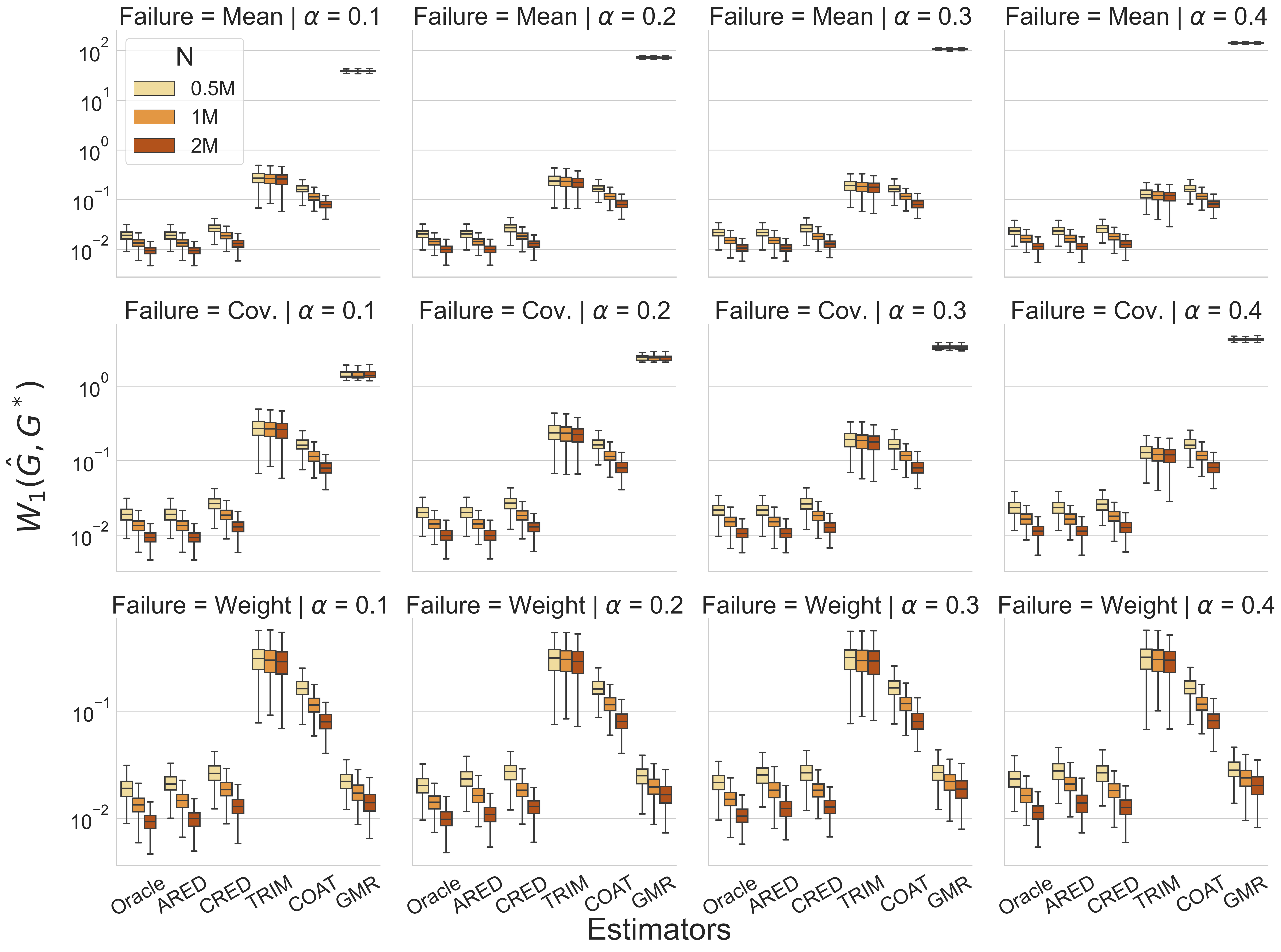
Under weight failure, both our CRED and ARED estimators remain highly competitive with the oracle estimator. Interestingly, GMR also works well, whereas other estimators perform poorly, with TRIM being particularly ineffective. The suboptimal performance of TRIM is largely due to its ignorance to the mixing weights in detecting potential Byzantine failures.

Statistical performance when the number of local machines scale up.

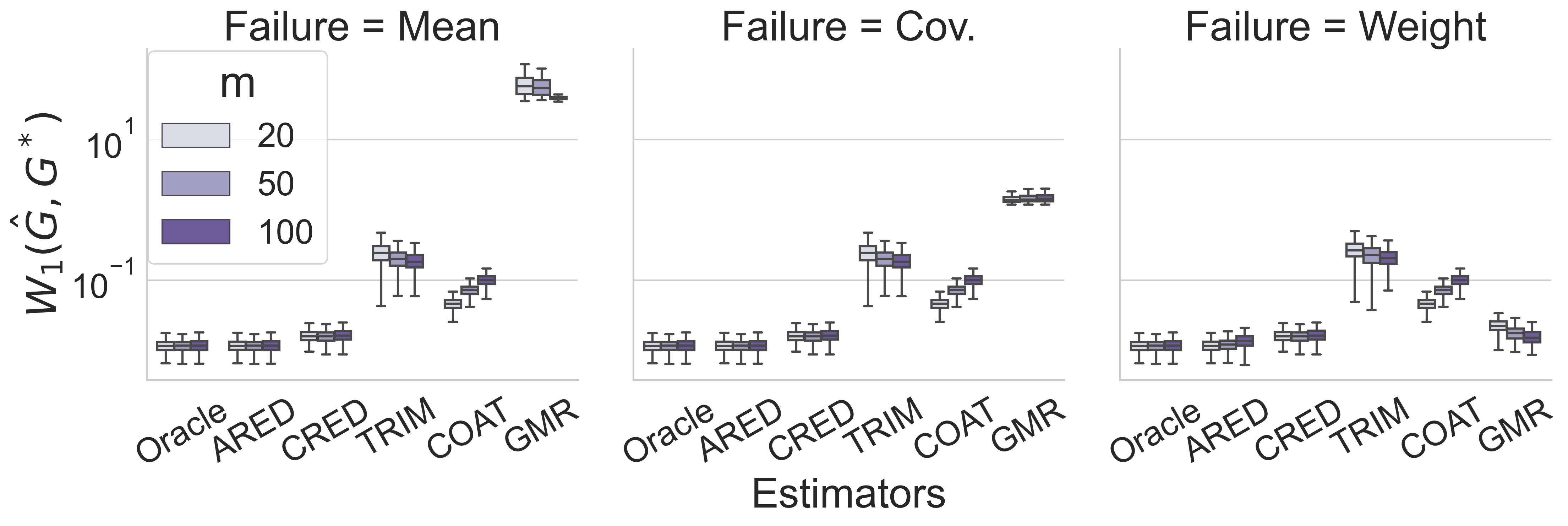
In addition to sample sizes, the scalability of the estimators in terms of the number of local machines ($m$) is crucial in distributed learning. Figures 3 and 4 show the $W_{1}$ values of various estimators as $m$ increases in a representative scenario where MaxOmega$=0.3$ and $\alpha=0.1$, under various failure scenarios.

We examine two cases: first, where the local machine sample size $n$ is fixed, as illustrated in Figure 3, and second, where the total sample size $N$is fixed, as shown in Figure 4. In both cases, the relative performance of different methods aligns with the findings in the previous setting. Our proposed CRED and ARED estimators consistently outperform other approaches.

Figure 3: $W_{1}$ values of different methods as $m$ varies, with $\alpha=0.1$, and MaxOmega$=0.3$. The local sample size $n=5000$, the total sample $N=nm$ increasing with $m$.

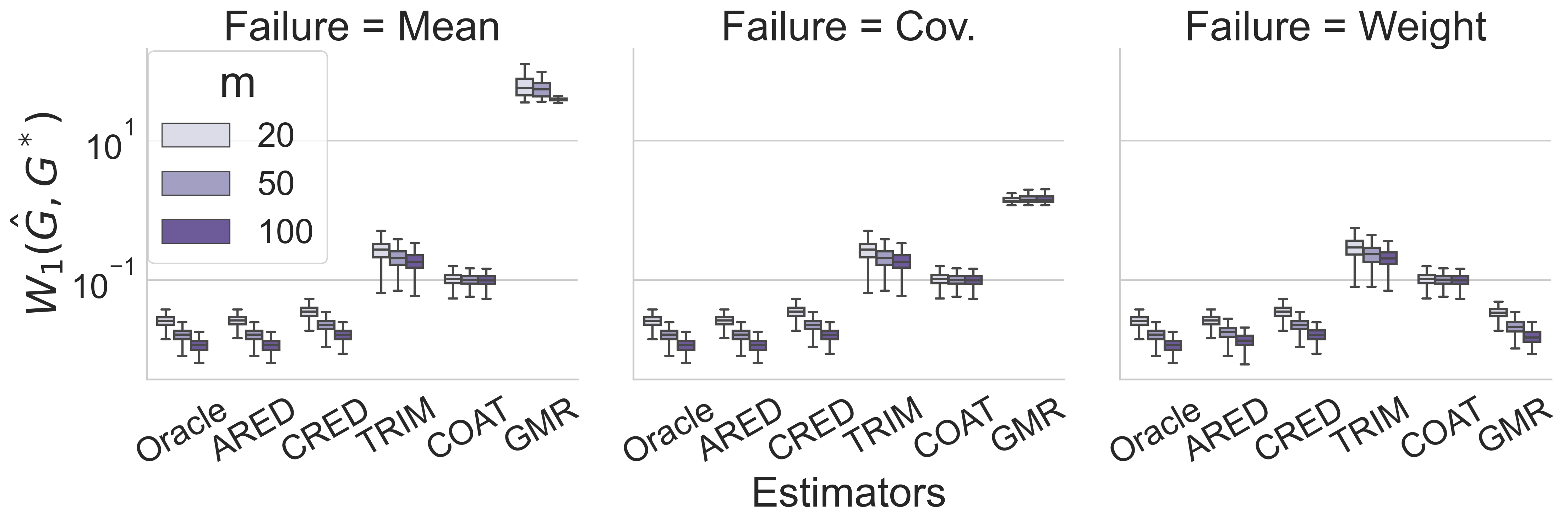
In the first case where the total sample size increases with more machines, the performance of the proposed methods improves. This is anticipated as our proposed estimators are consistent. In the second case where the total sample size does not increase with more machines, the performance of the proposed methods does not change with different number of machines. In comparison, the performance of COAT is determined solely by the local sample size $n$.

Figure 4: $W_{1}$ values of different methods as $m$ varies, with $\alpha=0.1$, and MaxOmega$=0.3$. The total sample size $N=500K$, the local sample $n=N/m$ decreasing with $m$.

Statistical performance with different degree of overlaps.

We next examine the performance of different approaches while varying the degree of overlap (MaxOmega). Figure 5 illustrates the $W_{1}$ of different methods in a representative case where $\alpha=0.2$, $m=100$, and local sample size $n=5000$, under various failure scenarios.

Figure 5: The $W_{1}$ of different methods as the degree of overlap MaxOmega varies, with $\alpha=0.2$, $m=100$, and local sample size $n=5000$, under various failure scenarios.

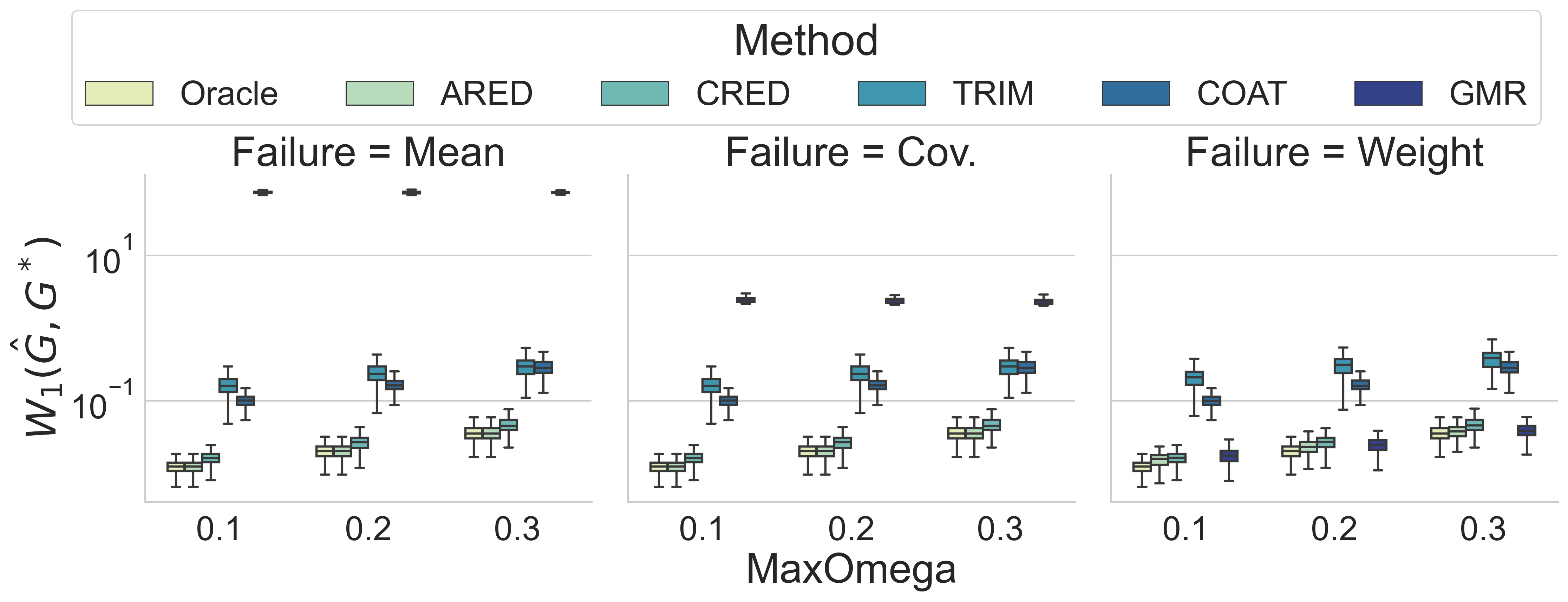
Our estimators remain comparable to the oracle estimator, irrespective of the failure type and degree of overlap. Other methods do not compete effectively with the proposed methods.

6 Real data analysis

In this section, we demonstrate Byzantine-tolerant aggregation of finite Gaussian mixtures for clustering on the well-known NIST dataset for digit recognition (Grother and Hanaoka, 2016).

We use the second edition of the dataset . It comprises approximately 4 million images of handwritten digits and characters (0–9, A–Z, and a–z) by different writers, partitioned into training and test sets. Figure 6(a) gives example images in the dataset. The number of training images for each digit and letter A–J are listed in Table 1.

Table 1: Numbers of training images in the NIST dataset.

Digits	0	1	2	3	4	5	6	7	8	9
Training	34803	38049	34184	35293	33432	31067	34079	35796	33884	33720
Test	5560	6655	5888	5819	5722	5539	5858	6097	5695	5813
Letter	A	B	C	D	E	F	G	H	I	J
Training	7010	4091	11315	4945	5420	10203	2575	3271	13179	3962

Each image is a $128\times 128$ pixel grayscale matrix, with entries ranging from $0$ to $1$, representing the darkness of the corresponding pixels, where a darker pixel has a value closer to $1$. We reduce each image to a $d=50$ real valued vector via deep convolutional neural network. Further details of the datasets and the architecture of the neural network are provided in Appendix C.3. Included in Figure 6(b) is the t-SNE visualization of the $50$-dimensional features of randomly selected samples in the dataset. The green and red dots are randomly selected digits and letters respectively. It is evident that features of the same digit or the same letter are clustered. Given this, an approach to build digit recognizer is to regard the features of each digit as a random sample from a distinct Gaussian distribution. Thus, the pooled data forms a sample from a finite Gaussian mixture of order $K=10$.

(a) Raw data.

(b) t-SNE visualization.

Figure 6: Random examples of digits and letters in the NIST dataset.

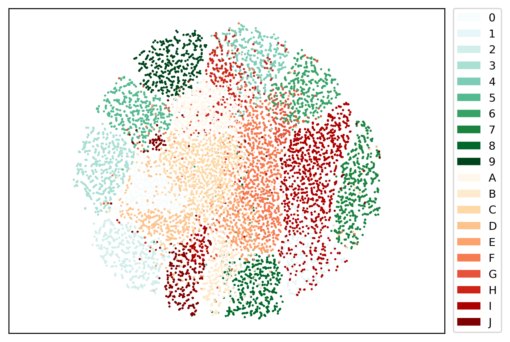
For illustration, we randomly select a dataset of size $N=25000$ and partition the dataset into $m=50$ subsets. We train an order $K=10$ Gaussian mixture model on each local machine. Afterward, we introduce Byzantine failure to a number of local estimates in a specific way. For each Byzantine failure machine, we independently obtain $n=5000$ random images of letters A–J and fit an order $K=10$ mixture to this data. We then replace the mixture on the corresponding Byzantine failure machine with this fitted mixture. Note that in Figure 6(b), the letter features are distinct from digit features and thus serve as a natural Byzantine failure. This procedure is repeated $R=300$ times.

We use the estimators in Section 5.2 for $\alpha\in\{0.0,0.1,0.2,0.3,0.4\}$. These mixture estimates are then employed to cluster images of handwritten digits in the test set. The ARI between the true label of the image and the predicted cluster label is given in Table 2.

Table 2: Median (IQR) ARI on the NIST digits test set of different methods under different failure rates.

$\alpha$	Oracle	ARED	CRED	TRIM	COAT	GMR
0.0	——	0.9197 (0.0014)	0.9188 (0.0020)	0.8704 (0.0423)	0.8616 (0.0158)	0.9197 (0.0014)
0.1	0.9195 (0.0014)	0.9195 (0.0014)	0.9188 (0.0018)	0.8761 (0.0469)	0.8624 (0.0148)	0.8827 (0.0116)
0.2	0.9194 (0.0015)	0.9194 (0.0015)	0.9187 (0.0020)	0.8796 (0.0496)	0.8618 (0.0167)	0.8674 (0.0141)
0.3	0.9194 (0.0015)	0.9194 (0.0015)	0.9188 (0.0021)	0.8866 (0.0422)	0.8616 (0.0158)	0.8541 (0.0113)
0.4	0.9190 (0.0018)	0.9190 (0.0019)	0.9187 (0.0019)	0.9050 (0.0454)	0.8600 (0.0174)	0.8449 (0.0127)

Our proposed ARED estimator completely matches the performance of the Oracle estimator in all cases. An intermediate step of ARED is to detect the Byzantine failure machines. We find that the ARED method detects $0.0000$, $0.0999$, $0.2000$, $0.3000$, and $0.3986$ when the true failure rate is $\alpha=0$, $0.1$, $0.2$, $0.3$, and $0.4$ respectively. The nearly perfect performance in this step explains why ARED matches the performance of the Oracle estimator. Our CRED is nearly as outstanding despite only utilizing $50\%$ of local estimates.

7 Discussion and concluding remarks

We propose two Byzantine-tolerant aggregation approaches, namely CRED and ARED, for distributed learning of finite mixture models. We show theoretically that both approaches are Byzantine-tolerant. Moreover, we show that ARED approach is able to detect Byzantine failure machines consistently under some general conditions. Our experiments show that both estimators has good performance statistically. Notably, the performance of ARED is nearly as perfect as the Oracle estimator.

Our work is an initial exploration into Byzantine-tolerant aggregation approaches for finite mixture models. There are numerous avenues for future research in this area. One compelling scenario, particularly relevant to mixture models, involves failures occurring at the component level rather than the machine level. This would result in more than half of the machines being faulty, while still retaining more than half of the failure-free estimates for each component. Exploring this scenario remains a promising direction for future investigation.

Appendix A Numerical algorithms

A.1 EM algorithm

The Maximum Likelihood Estimate (MLE) is commonly employed for local inference under finite mixture models. The preferred method for numerically computing MLE is the Expectation–Maximization (EM) algorithm. The EM algorithm is most conveniently described using the latent variable interpretation of the mixture.

For the $j$th unit with an observed value $x_{ij}$ from the finite mixture $f_{G}(x)$ on the $i$th machine, there exists a latent variable $z_{ij}$ associated with the observed value. When the latent variables $\{z_{ij},j\in[m]\}$ are known, we have the complete dataset $\{(z_{ij},x_{ij})\}$. This leads to the complete data log-likelihood function:

$$\ell_{n}^{c}(G)=\sum_{j=1}^{n}\sum_{k=1}^{K}\mathbbm{1}(z_{ij}=k)\log\{w_{k}f(x_{ij};\theta_{k})\}.$$

However, the complete data log-likelihood cannot be directly used to estimate $G$ because the latent variables are not known. In the EM algorithm iteration, one first replaces $z_{ij}$ in the complete data log-likelihood by its conditional expectation in each iteration. Let $G^{(t)}$ be the value of the mixing distribution after $t$-iteration. The conditional probability of $z_{ij}$ given the observed data is given by:

$$w_{ijk}^{(t)}={\mathbb{P}}(z_{ij}=k|G^{(t)},{\mathcal{X}})=\dfrac{w_{k}^{(t)}f(x_{ij};\theta_{k}^{(t)})}{\sum_{k^{\prime}=1}^{K}w_{k^{\prime}}^{(t)}f(x_{ij};\theta_{k^{\prime}}^{(t)})}.$$ (6)

The conditional expectation of $\ell_{n}^{c}(G)$ is then given by:

$$Q(G|G^{(t)})=\sum_{j=1}^{n}\sum_{k=1}^{K}w_{ijk}^{(t)}\log\{w_{k}f(x_{ij};\theta_{k})\}.$$

This is known as the E step of the algorithm.

Instead of seeking the maximizer of the complete data log-likelihood $\ell_{m}^{c}(G)$, the M step of the algorithm seeks the maximizer of $Q(G|G^{(t)})$ for $G\in{\mathbb{G}}_{K}$. This task is simpler since the subpopulation parameters $\theta_{k}$ are well separated in $Q(G|G^{(t)})$. The mixing distribution $G^{(t+1)}$ that maximizes $Q(G|G^{(t)})$ is composed of mixing weights:

$$w_{k}^{(t+1)}=n^{-1}\sum_{j=1}^{n}w_{ijk}^{(t)}$$

and subpopulation parameters:

$$\theta_{k}^{(t+1)}=\operatorname*{arg\,max}_{\theta}\left\{\sum_{j=1}^{n}w_{ijk}^{(t)}\log f(x_{ij};\theta)\right\}.$$

The EM iteration leads to another mixing distribution $G^{(t+1)}$. For many parametric subpopulation models ${\mathcal{F}}$, there is an analytical solution to $\theta_{k}^{(t+1)}$. Hence, the EM iteration is often straightforward to execute. Repeating the iteration leads to a sequence of mixing distributions. Under some conditions, Wu (1983) shows that $\ell_{m}(G^{(t)})=\sum_{j=1}^{m}\log f_{G^{(t)}}(x_{ij})$ is an increasing sequence, and the mixing distribution sequence $\{G^{(t)},t=1,2,\ldots\}$ converges to a local maximum of the log-likelihood function.

The EM algorithm suffers from a slow algorithmic convergence rate in general, and it can easily be trapped in local maxima. Various approaches (Meilijson, 1989; Meng and Rubin, 1993; Liu and Rubin, 1994; Balakrishnan et al., 2017) have been proposed to speed up convergence. However, we do not provide a review on this issue.

The MLE is not well-defined for the most widely used finite Gaussian mixtures and finite location-scale mixtures in general. Many variations are proposed to overcome this obstacle. For example, Hathaway (1985) proposes a constrained maximum likelihood formulation that seeks to avoid the unboundedness of the likelihood function. The resulting estimator has the desired consistency properties. However, this approach alters the parameter space and is undesirable. Ridolfi and Idier (2001) proposes to overcome the issue of the unbounded likelihood function through a Bayesian approach by posing an inverse gamma prior on the scale parameter under the Gaussian mixture models. The posterior mode is recommended as the MAP estimator. This MAP estimator, which can be regarded as a pMLE from the frequentist angle, is later shown to be consistent by Chen et al. (2008).

In Chen et al. (2008), a penalized log-likelihood function is defined as:

$$p\ell_{n}(G)=\ell_{n}(G)-a_{n}\sum_{k=1}^{K}p(\theta_{k})$$

for some penalty function $p(\cdot)$ and a parameter $a_{n}>0$ controls the strength of the penalty. The pMLE then becomes:

$$\widehat{G}^{\text{pMLE}}=\operatorname*{arg\,sup}_{G\in{\mathbb{G}}_{K}}p\ell_{n}(G)$$

Note that the penalty function is a sum of penalties applied to individual subpopulation parameters. This property is important to ensure easy implementation of the subsequent altered EM algorithm.

Three recommended penalty functions for different mixtures of ${\mathcal{F}}$ are:

• Under finite Gaussian mixtures, let $S_{x}$ be the sample covariance matrix of ${\mathcal{X}}_{i}$. Chen and Tan (2009) recommends the penalty function to be

  $$p(\theta)=\text{tr}(\Sigma^{-1}S_{x})+\log\text{det}(\Sigma)$$

  where $\text{tr}(\cdot)$ is the trace of a square matrix. The penalty function reduces to $p(\theta)=s_{x}^{2}/\sigma^{2}+\log\sigma^{2}$ under univariate Gaussian mixtures (Chen et al., 2008).

• Under finite location-scale mixtures with location parameter $\mu$ and scale parameter $\sigma$, one may replace the sample variance $s_{x}^{2}$ in the previous penalty function by a scale-invariant statistic. One such candidate is the squared sample interquartile range. This is helpful if the variance of $f_{0}(\cdot)$ is not finite.

• Under finite mixture of two-parameter Gamma distributions, the likelihood is also unbounded. Penalizing the likelihood is an effective way to restore statistical consistency. Chen et al. (2016) recommends the penalty function to be $p(\theta)=r-\log r$ where $r$ is the shape parameter in the Gamma distribution.

The EM algorithm can be easily adapted to compute the pMLE with the recommended penalty function (Chen and Tan, 2009). Employing the same latent variable interpretation as provided earlier, the penalized complete data log-likelihood is given by:

$$p\ell_{n}^{c}(G)=\sum_{j=1}^{n}\sum_{k=1}^{K}\mathbbm{1}(z_{ij}=k)\log\{w_{k}f(x_{ij};\theta_{k})\}-a_{n}\sum_{k=1}^{K}p(\theta_{k})$$

The only random quantity in $p\ell_{n}^{c}(G)$ is $\{z_{ijk},j\in[n],k\in[K]\}$ when conditioning on ${\mathcal{X}}_{i}$. Therefore, the conditional expectation calculation in (6) remains valid. The conditional expectation of $\ell_{n}^{c}(G)$ is then given by:

$$Q(G|G^{(t)})=\sum_{j=1}^{n}\sum_{k=1}^{K}w_{ijk}^{(t)}\log\{w_{k}f(x_{ij};\theta_{k})\}-a_{n}\sum_{k=1}^{K}p(\theta_{k}).$$

This completes the E step. The M step involves maximizing the above $Q(G|G^{(t)})$ that includes a penalty term. With the recommended penalty function, the subpopulation parameters remain well separated. It is evident that:

$$w_{k}^{(t+1)}=n^{-1}\sum_{j=1}^{n}w_{ijk}^{(t)}$$

and the updated subpopulation parameters become:

$$\theta_{k}^{(t+1)}=\operatorname*{arg\,max}_{\theta}\left\{\sum_{j=1}^{n}w_{ijk}^{(t)}\log f(x_{ij};\theta)-a_{n}p(\theta)\right\}.$$ (7)

Under Gaussian mixtures (Chen and Tan, 2009), the solution to (7) has the following form:

$$\begin{split}\mu_{k}^{(t+1)}&=\big{\{}nw_{k}^{(t+1)}\big{\}}^{-1}\sum_{j=1}^{n}w_{ijk}^{(t)}x_{ij},\\ \Sigma_{k}^{(t+1)}&=\big{\{}2a_{n}+nw_{k}^{(t+1)}\big{\}}^{-1}\big{\{}2a_{n}S_{x}+S_{k}^{(t+1)}\big{\}},\end{split}$$

where

$$S_{k}^{(t+1)}=\sum_{j=1}^{n}w_{ijk}^{(t)}(x_{ij}-\mu_{k}^{(t+1)})(x_{ij}-\mu_{k}^{(t+1)})^{\top}.$$

For a general location-scale mixture, the M step (7) does not always have a closed form solution. However, it only requires solving an optimization problem with two variables.

The EM algorithm for the pMLE, like its MLE counterpart, increases the value of the penalized likelihood after each iteration. For all $t$, we have $\Sigma_{k}^{(t)}\geq{2a_{n}/(m+2a_{n})}S_{x}>0$. The covariance matrices in $G^{(t)}$ have a lower bound that does not depend on the parameter values. This property ensures that the log-likelihood under Gaussian mixture at $G^{(t)}$ has a finite upper bound. Hence, the above iterative procedure is guaranteed to have $p\ell_{n}^{c}(G^{(t)})$ converge to at least a non-degenerate local maximum.

A.2 MM algorithm for GMR estimator

In this section, we summarize the Majorization Minimization (MM) algorithm for minimizing (2) in Zhang and Chen (2022) for reference. It starts with an initial $G^{\dagger}=\sum_{j=1}^{K}w^{\dagger}_{j}\delta_{\theta_{j}^{\dagger}}$, followed by alternating between two steps until convergence:

• Majorization step: Partition the support points of $\macc@depth\char 1\relax\frozen@everymath{\macc@group}\macc@set@skewchar\macc@nested@a 111{G}_{m}$, $\{\hat{\theta}_{ik}:i\in[m],k\in[K]\}$, into $K$ groups based on their closeness to $\theta_{j}^{\dagger}$. The $k$th component on $i$th machine belongs to the $j$th cluster if $c(\hat{\theta}_{ik},\theta_{j})\leq c(\hat{\theta}_{ik},\theta_{j^{\prime}})$ for any $j^{\prime}$.

• Update $\theta_{j}^{\dagger}$ by computing the barycenter of $\hat{\theta}_{ik}$ that belongs to $j$th cluster with respect to the cost function $c(\cdot,\cdot)$. Specifically, $\theta_{j}^{\dagger}=\operatorname*{arg\,min}_{\theta\in\Theta}\sum_{\{i,k:~{}\hat{\theta}_{ik}\in j\text{th cluster}\}}c(\hat{\theta}_{ik},\theta)$ and assign their mixing weights to $w^{\dagger}_{j}=\sum_{\{i,k:~{}\hat{\theta}_{ik}\in j\text{th cluster}\}}(n_{i}/N)\hat{w}_{ik}$.

Initialization: $f(\cdot;\theta^{\dagger}_{k})$, $k\in[K]$

repeat

     for $k\in[K]$ do

         Majorization: For $\gamma\in[mK]$, let

$$\pi_{\gamma k}=\begin{cases}(n_{\gamma}/N)\hat{w}_{\gamma}&\text{if}~{}k=\operatorname*{arg\,min}_{k^{\prime}}c(f(\cdot;\hat{\theta}_{\gamma}),f(\cdot;\theta^{\dagger}_{k^{\prime}}))\\ 0&\text{otherwise}\end{cases}$$

         Minimization: Let

$$\theta^{\dagger}_{k}=\operatorname*{arg\,min}_{\theta}\sum_{\gamma}\pi_{\gamma k}c(f(\cdot;\hat{\theta}_{\gamma}),f(\cdot;\theta))$$ (8)

     end for

until the change in $\sum_{\gamma,k}\pi_{\gamma k}c(f(\cdot;\hat{\theta}_{\gamma}),f(\cdot;\theta^{\dagger}_{k}))$ is below some threshold

Let $w^{\dagger}_{k}=\sum_{\gamma}\pi_{\gamma k}$

Output: $\sum_{k}w_{k}^{\dagger}f(\cdot;\theta^{\dagger}_{k})$

Algorithm 1 MM algorithm for GMR estimator under a general cost function $c(\cdot,\cdot)$.

The MM algorithm is summarized in Algorithm 1 for a general cost function $c(\cdot,\cdot)$ defined on ${\mathcal{F}}$. We order $\{\hat{\theta}_{ik}\}$ arbitrarily and use a single index $\gamma$ in the description for simplicity. When ${\mathcal{F}}=\{\phi(x;\mu,\Sigma)\}$ is the space of Gaussian distributions and the cost function is KL divergence:

$$c(\phi(x;\widehat{\mu}_{\gamma},\widehat{\Sigma}_{\gamma}),\phi(x;\mu^{\dagger}_{k},\Sigma^{\dagger}_{k}))= D_{\mathrm{KL}}(\phi(x;\widehat{\mu}_{\gamma},\widehat{\Sigma}_{\gamma})\|\phi(x;\mu^{\dagger}_{k},\Sigma^{\dagger}_{k}))$$

$$= -\log\phi(\widehat{\mu}_{\gamma};\mu^{\dagger}_{k},\Sigma^{\dagger}_{k})-\frac{1}{2}\Big{\{}\log\text{det}(2\pi\widehat{\Sigma}_{\gamma})-\mbox{tr}(\{\Sigma^{\dagger}_{k}\}^{-1}\widehat{\Sigma}_{\gamma})+d\Big{\}},$$

then the minimization step (8) can be obtained analytically via

$$\begin{split}&\mu^{\dagger}_{k}=\Big{\{}\sum_{\gamma}\pi_{\gamma k}\Big{\}}^{-1}\sum_{\gamma}\pi_{\gamma k}\widehat{\mu}_{\gamma},\\ &\Sigma^{\dagger}_{k}=\Big{\{}\sum_{\gamma}\pi_{\gamma k}\Big{\}}^{-1}\sum_{\gamma}\pi_{\gamma k}\{\widehat{\Sigma}_{\gamma}+(\widehat{\mu}_{\gamma}-\mu^{\dagger}_{k})(\widehat{\mu}_{\gamma}-\mu^{\dagger}_{k})^{\top}\}.\end{split}$$

A.3 Numerical algorithm for TRIM

In this section, we summarize the iterative algorithm for the TRIM estimator proposed in Del Barrio et al. (2019) for reference in Algorithm 2.

Initialization: $\{f(\cdot;\theta^{\ddagger}_{k})\}_{k=1}^{K}$, threshold $\eta\in(0,1)$

repeat

     for $\gamma\in[mK]$ do

         $c_{\gamma}=\operatorname*{arg\,min}_{j}c(f(\cdot;\tilde{\theta}_{\gamma}),f(\cdot;\theta^{\ddagger}_{j})),l_{\gamma}=c(f(\cdot;\tilde{\theta}_{\gamma}),f(\cdot;\theta^{\ddagger}_{c_{\gamma}}))$ $\triangleright$ Find the cluster assignment and compute its distance to the cluster center

     end for

     Find the permutation $\{(1),\ldots,(mK)\}$ such that $l_{(1)}\leq l_{(2)}\leq\cdots\leq l_{(mK)}$

     Set $\tau=\inf\{\eta\in[mK]:\sum_{\gamma=1}^{\eta}\tilde{w}_{(\gamma)}\leq 1-\eta\}$, let

$$\kappa_{\gamma}=\begin{cases}\tilde{w}_{(\gamma)}&\gamma<\tau\\ 1-\eta-\sum_{\gamma<\tau}\tilde{w}_{(\gamma)}&\gamma=\tau\\ 0&\text{otherwise}\end{cases}$$

$\triangleright$ Trimming

     for $k\in[K]$ do

         $\theta^{\ddagger}_{k}=\operatorname*{arg\,min}_{\theta}\sum_{\{\gamma:c_{\gamma}=k\}}\kappa_{\gamma}c(f(\cdot;\tilde{\theta}_{\gamma}),f(\cdot;\theta))$ $\triangleright$ Update cluster centers

         $w^{\ddagger}_{k}=(1-\eta)^{-1}\sum_{\{\gamma:c_{\gamma}=k\}}\kappa_{\gamma}\tilde{w}_{\gamma}$ $\triangleright$ Update weights

     end for

until there is no change in $c_{\gamma}$ for all $\gamma\in[mK]$

Output: $\sum_{k}w_{k}^{\ddagger}f(\cdot;\theta^{\ddagger}_{k})$

Algorithm 2 Iterative algorithm to compute the TRIM estimator in Del Barrio et al. (2019).

Appendix B Statistical Guarantees

In this section, we establish the statistical properties presented in Lemma 4.2, Lemma 4.3, and Theorem 4.1. We begin by introducing some notations within the context of finite mixture model specified in Definition 2.1. Let ${\bm{S}}_{11}^{*}$ be a ${(K-1)\times(K-1)}$ matrix with the $(k_{1},k_{2})$th element defined as

$${\bm{S}}_{11}^{*}[k_{1},k_{2}]=\int\{f(x;\theta_{k_{1}}^{*})-f(x;\theta_{K}^{*})\}\{f(x;\theta_{k_{2}}^{*})-f(x;\theta_{K}^{*})\}\,dx,$$

${\bm{S}}_{12}^{*}$ a ${(K-1)\times K}$ block matrix with the $(k_{1},k_{2})$th block being a length $p$ vector given by

$${\bm{S}}_{12}^{*}[k_{1},k_{2}]=\int w_{k_{2}}^{*}\{f(x;\theta_{k_{1}}^{*})-f(x;\theta_{K}^{*})\}\nabla_{\theta}^{\top}f(x;\theta_{k_{2}}^{*})\,dx,$$

and ${\bm{S}}_{22}^{*}$ a ${K\times K}$ block matrix with the $(k_{1},k_{2})$th block being a $p\times p$ matrix defined as

$${\bm{S}}_{22}^{*}[k_{1},k_{2}]=\int w_{k_{1}}^{*}w_{k_{2}}^{*}\nabla_{\theta}f(x;\theta_{k_{1}}^{*})\nabla_{\theta}^{\top}f(x;\theta_{k_{2}}^{*})\,dx.$$

We assume all integrations involved are finite. Denote

$${\bm{H}}^{*}=\begin{pmatrix}{\bm{S}}_{11}^{*}&{\bm{S}}_{12}^{*}\\ {\bm{S}}_{12}^{*\top}&{\bm{S}}_{22}^{*}\end{pmatrix}.$$

B.1 Preliminary results

The pairwise Integrated Squared Error (ISE) between two local estimates is a crucial quantity in our proposed methods. The following useful order assessments are obtained when the subpopulation density function $f(x;\theta)$, its derivatives with respect to $\theta$ up to order $2$ are square integrable. Commonly used subpopulation distributions, such as normal, clearly satisfy the square integrability condition.

Lemma B.1.

Let $\widehat{G}$ and $\widehat{G}^{\dagger}$ be two independent estimators of $G^{*}$ with properties described in Lemma 4.1. Denote $\widehat{{\bm{G}}}=(\hat{w}_{1},\ldots,\hat{w}_{K-1},\hat{\theta}_{1}^{\top},\ldots,\hat{\theta}_{K}^{\top})^{\top}$ and similarly for ${\bm{G}}$. Suppose that $f(x;\theta_{k})$, $\nabla_{\theta}f(x;\theta_{k})$, and $\nabla^{2}_{\theta}f(x;\theta_{k})$ are entry-wise bounded by a square integrable function $W(x)$ uniformly in a neighborhood of $\theta_{k}^{*}$. Then, as $n\to\infty$,

$$\begin{split}D_{\text{ISE}}^{2}(\widehat{G},G^{*})=&(\widehat{{\bm{G}}}-{\bm{G}}^{*})^{\top}{\bm{H}}^{*}(\widehat{{\bm{G}}}-{\bm{G}}^{*})+O_{p}(n^{-3/2}),\\ D_{\text{ISE}}^{2}(\widehat{G},\widehat{G}^{\dagger})=&2(\widehat{\bf G}-\widehat{\bf G}^{\dagger})^{\top}{\bm{H}}^{*}(\widehat{\bf G}-\widehat{\bf G}^{\dagger})+O_{p}(n^{-3/2}).\end{split}$$

Proof.

We first expand $f(x;\hat{\theta}_{k})$ at $\theta_{k}^{*}$ to get

$$f(x;\hat{\theta}_{k})=f(x;\theta_{k}^{*})+\nabla_{\theta}^{\top}f(x;\theta_{k}^{*})(\hat{\theta}_{k}-\theta_{k}^{*})+W(x)O_{p}(n^{-1}),$$

with the order of remainder term justified by $\widehat{\bm{G}}-{\bm{G}}^{*}=O_{p}(n^{-1/2})$ as in Lemma 4.1. Hence,

$$\begin{split}f_{\widehat{G}}(x)-f_{G^{*}}(x)=&\sum_{k=1}^{K-1}(\hat{w}_{k}-w_{k}^{*})\{f(x;\theta_{k}^{*})-f(x;\theta_{K}^{*})\}+\sum_{k=1}^{K}w_{k}^{*}\nabla_{\theta}^{\top}f(x;\theta_{k}^{*})(\hat{\theta}_{k}-\theta_{k}^{*})\\ &+W(x)O_{p}(n^{-1}).\end{split}$$

Note that the leading term is linear in $\widehat{\bm{G}}-{\bm{G}}^{*}$. Consequently, squaring the above expansion and integrating with respect to $x$, term by term, noting that $W(x)$ is square integrable, we get

$$\begin{split}D_{\text{ISE}}^{2}(\widehat{G},G^{*})=&\int\{f_{\widehat{G}}(x)-f_{G^{*}}(x)\}^{2}\,dx\\ =&2\int\Big{\{}\sum_{k=1}^{K-1}(\hat{w}_{k}-w_{k}^{*})f(x;\theta_{k}^{*})\Big{\}}\Big{\{}\sum_{k=1}^{K}w_{k}^{*}\nabla^{\top}f(x;\theta_{k}^{*})(\hat{\theta}_{k}-\theta_{k}^{*})\Big{\}}\,dx\\ &+\int\left\{\sum_{k=1}^{K-1}(\hat{w}_{k}-w_{k}^{*})\{f(x;\theta_{k}^{*})-f(x;\theta_{k}^{*})\}\right\}^{2}\,dx\\ &+\int\Big{\{}\sum_{k=1}^{K}w_{k}^{*}\nabla^{\top}f(x;\theta_{k}^{*})(\hat{\theta}_{k}-\theta_{k}^{*})\Big{\}}^{2}\,dx+O_{p}(n^{-3/2})\\ =&(\widehat{{\bm{G}}}-{\bm{G}}^{*})^{\top}{\bm{H}}^{*}(\widehat{{\bm{G}}}-{\bm{G}}^{*})+O_{p}(n^{-3/2}).\end{split}$$

This proves the first conclusion of the Lemma. The second conclusion follows the same logic. ∎

B.2 Proof of Lemma 4.2

Before the proof, it is helpful to recall that $\widehat{G}_{j}$ and $\widetilde{G}_{j}$ represent local estimators before and after transmission, respectively. It is important to keep in mind that none of $\widehat{G}_{j}$ are subject to Byzantine failure, whereas some of $\widetilde{G}_{j}$ may be.

Proof.

The first conclusion $D_{\text{ISE}}(\widehat{G},G^{*})=O_{p}(n^{-1/2})$ follows immediately from Lemma 4.1 and that $\widehat{{\bm{G}}}-{\bm{G}}^{*}=O_{p}(n^{-1/2})$. We rewrite the expansion in Lemma B.1 in the form:

$$nD_{\text{ISE}}^{2}(\widehat{G},G^{*})=\{\sqrt{n}(\widehat{{\bm{G}}}-{\bm{G}}^{*})\}^{\top}{\bm{H}}^{*}\{\sqrt{n}(\widehat{{\bm{G}}}-{\bm{G}}^{*})\}+O_{p}(n^{-1/2}).$$

We show below that the first term is dominated by a chi-squared distribution and is of order $O_{p}(1)$, making the conclusion $D_{\text{ISE}}(\widehat{G},G^{*})=O_{p}(n^{-1/2})$ obvious.

Let ${\bm{Z}}$ be standard normally distributed of dimension $Kp+K-1$. By Lemma 4.1,

$$\sqrt{n}{\bm{I}}^{1/2}(G^{*})(\widehat{{\bm{G}}}-{\bm{G}}^{*})\overset{d}{\to}{\bm{Z}}.$$

Hence, denoting ${\bm{I}}={\bm{I}}(G^{*})$,

$$nD_{\text{ISE}}^{2}(\widehat{G},G^{*})\overset{d}{\to}{\bm{Z}}^{\top}\{{\bm{I}}^{-1/2}{\bm{H}}^{*}{\bm{I}}^{-1/2}\}{\bm{Z}}.$$

It is seen that ${\bm{Z}}^{\top}\{{\bm{I}}^{-1/2}{\bm{H}}^{*}{\bm{I}}^{-1/2}\}{\bm{Z}}$ is stochastically dominated by $\rho\chi^{2}_{Kp+K-1}$ where $\rho$ is the maximum eigenvalue of ${\bm{I}}^{-1/2}{\bm{H}}^{*}{\bm{I}}^{-1/2}$ that only depends on $G^{*}$. That is, for all $t>0$,

$${\mathbb{P}}({\bm{Z}}^{\top}\{{\bm{I}}^{-1/2}{\bm{H}}^{*}{\bm{I}}^{-1/2}\}{\bm{Z}}\geq t)\leq{\mathbb{P}}(\rho\chi^{2}_{Kp+K-1}\geq t).$$

Note the density function of $\chi^{2}_{Kp+K-1}$ is proportional to $t^{(Kp+K-1)/2-1}\exp(-t/2)$. It is therefore elementary to show that ${\mathbb{P}}(\chi^{2}_{Kp+K-1}>t)<C\exp(-t/(2+\epsilon))$ for any $\epsilon>0$, with a generic $C$ and corresponding sufficiently large $t$. Hence, let $\epsilon=1$ and for large $t$,

$${\mathbb{P}}(\rho\chi^{2}_{Kp+K-1}\geq t)\leq C\exp\left(-\frac{t}{3\rho}\right).$$

We can also use Hanson-Wright Inequality in Vershynin (2018, Section 6.2) to upper bound the probability ${\mathbb{P}}({\bm{Z}}^{\top}\{{\bm{I}}^{-1/2}{\bm{H}}^{*}{\bm{I}}^{-1/2}\}{\bm{Z}}\geq t)$. We find our proof here is much simplified for the purpose of characterizing the order of $D_{\text{ISE}}$.

Given the limiting conclusion, we therefore have

$${\mathbb{P}}(nD_{\text{ISE}}^{2}(\widehat{G},G^{*})\geq t)\leq C\exp\left(-\frac{t}{3\rho}\right)$$

for some positive constants $\rho$ and $C$, applicable to all sufficiently large $t$. Consequently, let $M^{2}>6\rho$ and when $m$ is sufficiently large, we have

$$\begin{split}{\mathbb{P}}\Big{(}\max_{i\in[m]}D_{\text{ISE}}(\widehat{G}_{i},G^{*})\geq Mn^{-1/2}\sqrt{\log m}\Big{)}\leq&m{\mathbb{P}}\Big{(}nD_{\text{ISE}}^{2}(\widehat{G}_{i},G^{*})\geq M^{2}\log m\Big{)}\\ \leq&Cm\exp(-2\log m)=C/m\end{split}$$

which goes to zero as $m\to\infty$. In other words,

$$\max_{i\in[m]}D_{\text{ISE}}(\widehat{G}_{i},G^{*})=O_{p}(n^{-1/2}\sqrt{\log m}).$$

By triangle inequality, we further conclude

$$\max_{i,j\in[m]}D_{\text{ISE}}(\widehat{G}_{i},\widehat{G}_{j})=O_{p}(n^{-1/2}\sqrt{\log m}).$$

Because when $i\not\in{\mathbb{B}}^{*}$, $\widetilde{G}_{i}=\widehat{G}_{i}$, it implies

$$\max_{i,j\not\in{\mathbb{B}}^{*}}D_{\text{ISE}}(\widetilde{G}_{i},\widetilde{G}_{j})=O_{p}(n^{-1/2}\sqrt{\log m}).$$

Taking maximum inflates the order by a scale factor $\sqrt{\log m}$. ∎

B.3 Proof of Lemma 4.3

Proof.

Based on the proof of the order for $\max_{i,j\not\in{\mathbb{B}}^{*}}D_{\text{ISE}}(\widetilde{G}_{i},\widetilde{G}_{j})$ in Lemma 4.2, to establish the result in this lemma, we only need to show that for any $M$,

$${\mathbb{P}}\left(\min_{i\in{\mathbb{B}}^{*},j\not\in{\mathbb{B}}^{*}}D_{\text{ISE}}(\widetilde{G}_{i},\widetilde{G}_{j})\geq Mn^{-1/2}\sqrt{\log m}\right)\to 1.$$

We prove a stronger claim by replacing $Mn^{-1/2}\sqrt{\log m}$ by $n^{-1/2}\log^{2}m$ for the sake for future reference. Based on the triangle inequality, we have

$$D_{\text{ISE}}(\widetilde{G}_{i},\widetilde{G}_{j})\geq D_{\text{ISE}}(\widetilde{G}_{i},G^{*})-D_{\text{ISE}}(G^{*},\widetilde{G}_{j}).$$

Note that when $i\in{\mathbb{B}}^{*}$ but $j\not\in{\mathbb{B}}^{*}$, the problem reduces to show that as $n,m\to\infty$

$${\mathbb{P}}\Big{(}\min_{i\in{\mathbb{B}}^{*}}D_{\text{ISE}}(\widetilde{G}_{i},G^{*})>n^{-1/2}{\log^{2}m}\Big{)}\to 1.$$

Fix a $j\in{\mathbb{B}}^{*}$, it is seen

$${\mathbb{P}}\Big{(}\min_{i\in{\mathbb{B}}^{*}}D_{\text{ISE}}(\widetilde{G}_{i},G^{*})>n^{-1/2}{\log^{2}m}\Big{)}=\Big{\{}{\mathbb{P}}\Big{(}D_{\text{ISE}}(\widetilde{G}_{j},G^{*})>n^{-1/2}{\log^{2}m}\Big{)}\Big{\}}^{m}.$$

By the characterizing assumption on the Byzantine failure estimator, we get

$${\mathbb{P}}\Big{(}D_{\text{ISE}}(\widetilde{G}_{j},G^{*})>n^{-1/2}{\log^{2}m}\Big{)}\geq 1-(n^{-1/2}\log^{2}m)^{\gamma}=1-O(n^{-\gamma/2}(\log m)^{2\gamma}).$$

Under the conditions $m=O(N^{\beta})$ and $\gamma>2\beta/(1-\beta)$, we have

$$\begin{split}&{\mathbb{P}}\Big{(}\min_{i\in{\mathbb{B}}^{*}}D_{\text{ISE}}(\widetilde{G}_{i},G^{*})>n^{-1/2}{\log^{2}m}\Big{)}\geq(1-Cn^{-\gamma/2}(\log m)^{2\gamma})^{m}\\ =&\exp(-Cmn^{-\gamma/2}(\log m)^{2\gamma})=\exp(-CN^{\beta-\gamma(1-\beta)/2}(\log N)^{2\gamma})\to 1\end{split}$$

Hence,

$${\mathbb{P}}\Big{(}\min_{i\in{\mathbb{B}}^{*}}D_{\text{ISE}}(\widetilde{G}_{i},G^{*})>n^{-1/2}{\log^{2}m}\Big{)}\geq 1+o(1),$$

which completes the proof. ∎

B.4 Proof of Theorem 4.1

Proof.

We give the proof of the three conclusions in Theorem 4.1 below.

• This result states that $\widehat{G}^{\mbox{\tiny{COAT}}}$ is Byzantine failure-free. Denote

  $$r=\max_{i,j\not\in{\mathbb{B}}^{*}}D_{\text{ISE}}(\widetilde{G}_{i},\widetilde{G}_{j}).$$

  Since $\text{Card}({\mathbb{B}}^{*})<0.5m$, it follows that for any $i\not\in{\mathbb{B}}^{*}$, $\widetilde{G}_{i}$ has more than $0.5m$ local estimators within its $r$-distance. By the definition of $r^{\mbox{\tiny{COAT}}}$, we have $r^{\mbox{\tiny{COAT}}}\leq r$. According to Lemma 4.3, for any given $j_{0}\in{\mathbb{B}}^{*}$, none of $\widetilde{G}_{i}$ with $i\not\in{\mathbb{B}}^{*}$ is within $r$-distance of $\widetilde{G}_{j_{0}}$. Given $\text{Card}({\mathbb{B}}^{*})<0.5m$, there are fewer than $0.5m$ $\widetilde{G}_{i}$ within $r^{\mbox{\tiny{COAT}}}$ distance from $\widetilde{G}_{j_{0}}$. Hence, with probability approaching 1, $\widetilde{G}_{j_{0}}$ is not $\widehat{G}^{\mbox{\tiny{COAT}}}$.

• In part (a), we have established that $\widehat{G}^{\text{coat}}$ is not a Byzantine estimator with probability approaching 1. By Lemma 4.3, this implies that all non-Byzantine estimators are within $r$-distance of $\widehat{G}^{\text{coat}}$, whereas all Byzantine estimators are more than $r$-distance away. Therefore, the closest 50% of local estimators to $\widehat{G}^{\text{coat}}$ exclusively consist of Byzantine failure-free estimators, as concluded in part (b).

• Denote

  $$\tilde{r}^{2}_{N}=\frac{1}{2}\log\left(\frac{m}{2}\right)\log\log(m)(r^{\mbox{\tiny{COAT}}})^{2}.$$

  Claim (c) holds if:

  • For every $j\in{\mathbb{B}}^{*}$, $D_{\text{ISE}}^{2}(\widetilde{G}_{j},\widehat{G}^{\mbox{\tiny{COAT}}})>\tilde{r}^{2}_{N}$;

  • For every $i\not\in{\mathbb{B}}^{*}$, $D_{\text{ISE}}^{2}(\widetilde{G}_{i},\widehat{G}^{\mbox{\tiny{COAT}}})<\tilde{r}^{2}_{N}$.

  Thus, the validity of (c) depends on the order of $\tilde{r}^{2}_{N}$.

  According to the proof of (b), with probability approaching $1$,

  $$r^{\mbox{\tiny{COAT}}}\leq\max_{i,j\not\in{\mathbb{B}}^{*}}D_{\text{ISE}}(\widetilde{G}_{i},\widetilde{G}_{j})=O_{p}(n^{-1/2}\sqrt{\log m})$$

  with the order given by Lemma 4.2. Hence, after omitting unimportant constants,

  $$\tilde{r}_{N}=O_{p}(n^{-1/2}\log(m)\sqrt{\log\log(m)}).$$

  At the same time, because $\widehat{G}^{\mbox{\tiny{COAT}}}$ is Byzantine failure-free in probability, we have that for any $i\in{\mathbb{B}}^{*}$, with probability approaching 1,

  $$D_{\text{ISE}}(\widetilde{G}_{i},\widehat{G}^{\mbox{\tiny{COAT}}})\geq\min_{i\in{\mathbb{B}}^{*},j\not\in{\mathbb{B}}^{*}}D_{\text{ISE}}(\widetilde{G}_{i},\widetilde{G}_{j})\geq n^{-1/2}\log^{2}m>\tilde{r}_{N},$$

  where the second last inequality is based on the proof in Lemma 4.3. This completes the first half of the proof: $\widehat{{\mathbb{B}}}^{\mbox{\tiny{ARED}}}$ includes all Byzantine estimators.

  It remains to show that $\widehat{{\mathbb{B}}}^{\mbox{\tiny{ARED}}}$ includes only Byzantine estimators. This is implied if

  $$\max_{i\not\in{\mathbb{B}}^{*}}D_{\text{ISE}}(\widetilde{G}_{i},\widehat{G}^{\mbox{\tiny{COAT}}})<\tilde{r}_{N}$$

  with probability approaching 1. By a simple inequality and Lemma 4.3, we have

  $$\max_{i\not\in{\mathbb{B}}^{*}}D_{\text{ISE}}(\widetilde{G}_{i},\widehat{G}^{\mbox{\tiny{COAT}}})\leq\max_{i,j\not\in{\mathbb{B}}^{*}}D_{\text{ISE}}(\widetilde{G}_{i},\widetilde{G}_{j})=O(n^{-1/2}\sqrt{\log m}).$$

  Hence, the conclusion holds when $\tilde{r}_{N}$ has an order larger than $n^{-1/2}\sqrt{\log m}$.

  Because $r^{\mbox{\tiny{COAT}}}$ is the distance between two independent non-Byzantine estimators, $r^{\mbox{\tiny{COAT}}}=O_{p}(n^{-1/2})$ in strict sense. Therefore, we have $r^{\mbox{\tiny{COAT}}}>n^{-1/2}(\log\log m)^{-1/4}$ in probability. Omitting a harmless scale constant, this leads to

  $$\tilde{r}_{N}\geq n^{-1/2}\sqrt{\log m}(\log\log m)^{1/4}.$$

  The right-hand-side exceeds $O(n^{-1/2}\sqrt{\log m})$. This completes the second half of the proof: $\widehat{{\mathbb{B}}}^{\mbox{\tiny{ARED}}}$ excludes all Byzantine estimators.

∎

Appendix C Experiments

C.1 More details

Under finite Gaussian mixtures, the ISE between $\phi_{G}(x)=\sum_{i}w_{i}\phi(x;\mu_{i},\Sigma_{i})$ and $\phi_{G^{\prime}}(x)=\sum_{j}w_{j}^{\prime}\phi(x;\mu_{j}^{\prime},\Sigma_{j}^{\prime})$ has the following convenient analytical expression:

$$D_{\text{ISE}}^{2}(G^{\prime},G)=\int\{\phi_{G^{\prime}}(x)-\phi_{G}(x)\}^{2}\,dx=w^{\top}S_{OO}w-2w^{\top}S_{OR}w^{\prime}+(w^{\prime})^{\top}S_{RR}(w^{\prime})$$

where $w=(w_{i})$, $w^{\prime}=(w^{\prime}_{j})$, and $S_{OO}$, $S_{OR}$, and $S_{RR}$ are matrices with their $(i,j)$-th elements respectively being $\phi(\mu_{i};\mu_{j},\Sigma_{i}+\Sigma_{j})$, $\phi(\mu_{i};\mu_{j}^{\prime},\Sigma_{i}+\Sigma_{j}^{\prime})$, and $\phi(\mu_{i}^{\prime};\mu_{j}^{\prime},\Sigma_{i}^{\prime}+\Sigma_{j}^{\prime})$. The derivation of the analytical expression is due to the property

$$\int\phi(x;\mu_{1},\Sigma_{1})\phi(x;\mu_{2},\Sigma_{2})\,dx=\phi(\mu_{1};\mu_{2},\Sigma_{1}+\Sigma_{2})$$

for any two Gaussian densities.

We give the details of the performance metrics we used in the experiments. Let $G^{(r)}$ be the true mixing distribution in $r$th repetition and $\widehat{G}^{(r)}=\sum_{k}\widehat{w}_{k}^{(r)}\delta_{(\widehat{\mu}_{k}^{(r)},\widehat{\Sigma}_{k}^{(r)})}$ be an estimate. We assess the performance using the following metrics:

1. Transportation distance ($W_{1}$). Denote respectively by $\widehat{\phi}_{i}^{(r)}(x)=\phi(x;\widehat{\mu}_{i}^{(r)},\widehat{\Sigma}_{i}^{(r)})$ and $\phi_{j}^{(r)}(x)=\phi(x;\mu_{j}^{(r)},\Sigma_{j}^{(r)})$ and

   $$D_{1}(\widehat{\phi}_{i}^{(r)},\phi_{j}^{(r)})=\|\widehat{\mu}_{i}^{(r)}-\mu_{j}^{(r)}\|_{2}+\|(\widehat{\Sigma}_{i}^{(r)})^{1/2}-(\Sigma_{j}^{(r)})^{1/2}\|_{F}$$

   where $\Sigma^{1/2}\geq 0$ is the square root of $\Sigma\geq 0$ and $\|\Sigma\|_{F}=\sqrt{\text{tr}(\Sigma^{\top}\Sigma)}$ is the Frobenius norm of a matrix. The transportation distance between two mixing distributions is

   $$W_{1}(\widehat{G}^{(r)},G^{(r)})=\operatorname*{arg\,min}\left\{\sum_{ij}\pi_{ij}D_{1}(\widehat{\phi}_{i}^{(r)},\phi_{j}^{(r)}):\sum_{j}\pi_{ij}=\widehat{w}_{i}^{(r)},\sum_{i}\pi_{ij}=w_{j}^{(r)}\right\}$$

2. Adjusted Rand Index (ARI). Mixture models are often used for model-based clustering. For a given $G$, we can assign a unit with observed value $x$ to a cluster via:

   $$k(x)=\operatorname*{arg\,max}_{k}\{w_{k}\phi(x;\mu_{k},\Sigma_{k})\}.$$

   We measure the performance of the clustering results of the full dataset based on $\widehat{G}^{(r)}$ and $G^{(r)}$ by calculating the adjusted Rand index (ARI). The ARI is a well-known measure of the similarity between two clustering outcomes. Suppose that the observations in a dataset are divided into $K$ clusters $A_{1},A_{2},\ldots,A_{K}$ by one method and $K^{\prime}$ clusters $B_{1},B_{2},\ldots,B_{K^{\prime}}$ by another. Let $N_{i}=\text{Card}(A_{i}),~{}M_{j}=\text{Card}(B_{j}),~{}~{}N_{ij}=\text{Card}(A_{i}\cap B_{j})$ for $i\in[K]$ and $j\in[K^{\prime}]$. The ARI of these two clustering results is calculated as follows:

   $$\text{ARI}=\dfrac{\sum_{i,j}\binom{N_{ij}}{2}-\binom{N}{2}^{-1}\sum_{i,j}\binom{N_{i}}{2}\binom{M_{j}}{2}}{\frac{1}{2}\sum_{i}\binom{N_{i}}{2}+\frac{1}{2}\sum_{j}\binom{M_{j}}{2}-\binom{N}{2}^{-1}\sum_{i,j}\binom{N_{i}}{2}\binom{M_{j}}{2}}$$

   where $\binom{n}{k}$ is the number of combinations of $k$ from a given set of $n$ elements. A value close to 1 for the ARI indicates a high degree of agreement between the two clustering methods, and it is equal to 1 when the two methods completely agree.

C.2 More simulation results

In this section, we present the performance of various methods in terms of ARI. The relative performance of the estimators in terms of ARI mirros that of $W_{1}$.

Figure 7 corresponds to the settings in Figure 2.

Figure 7: The ARI of clustering results based on the full dataset as $N$ and $\alpha$ varies, with $m=100$ and MaxOmega$=0.3$.

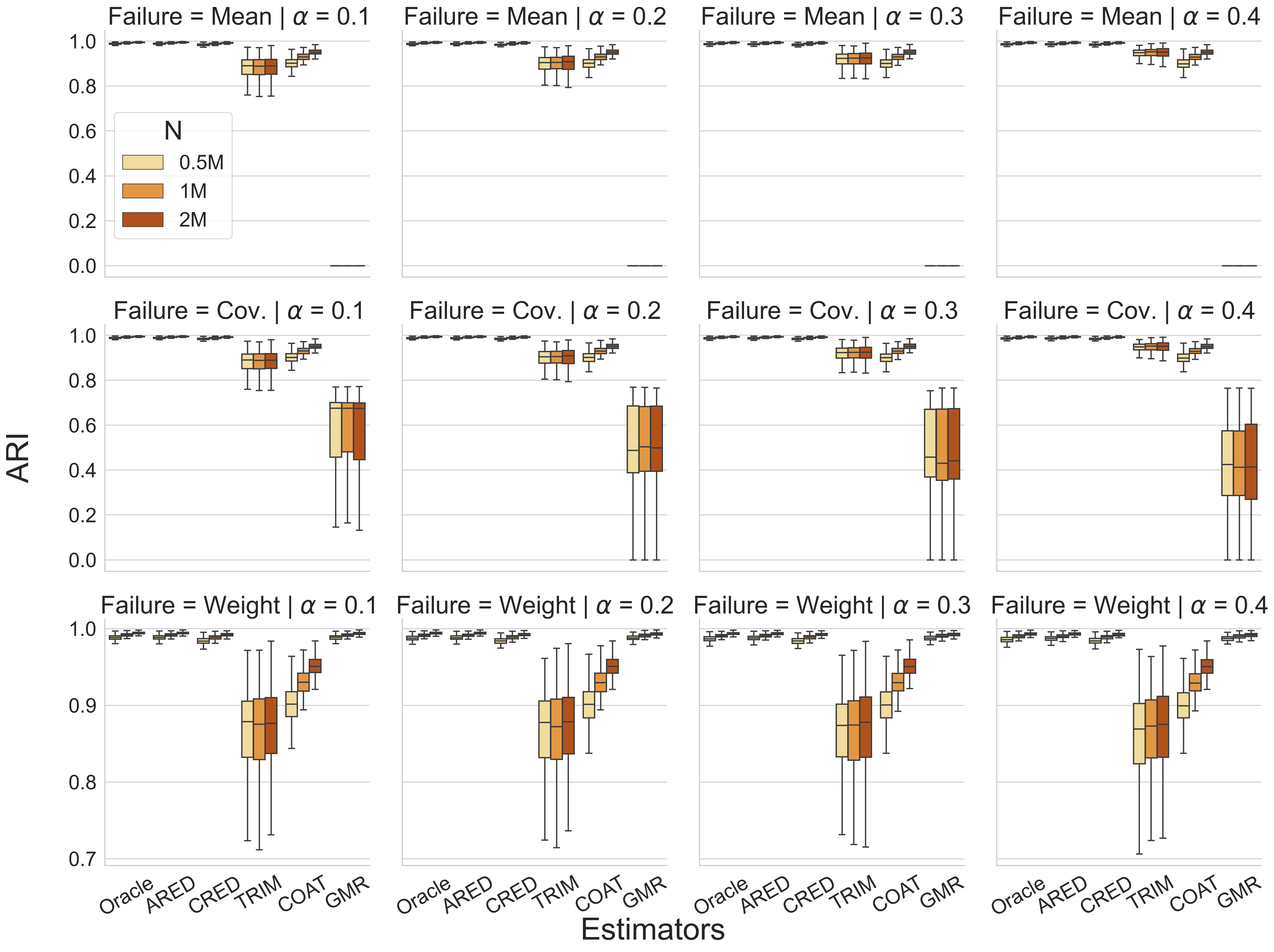
Figures 8 and 9 correspond to the settings in Figures 3 and Figure 4, respectively. The y-axis is constrained to $[0.8,1.0]$ to better illustrate differences among estimators. The GMR estimator has a low ARI under mean and covariance attacks, and is omitted in the first two panels in both.

Figure 8: The ARI of clustering results based on the full dataset as $m$ varies, with $\alpha=0.1$, and MaxOmega$=0.3$. The local sample size $n=5000$, the total sample $N=nm$ increasing with $m$.

Figure 9: The ARI of clustering results based on the full dataset as $m$ varies, with $\alpha=0.1$, and MaxOmega$=0.3$. The total sample size $N=500K$, the local sample $n=N/m$ decreasing with $m$.

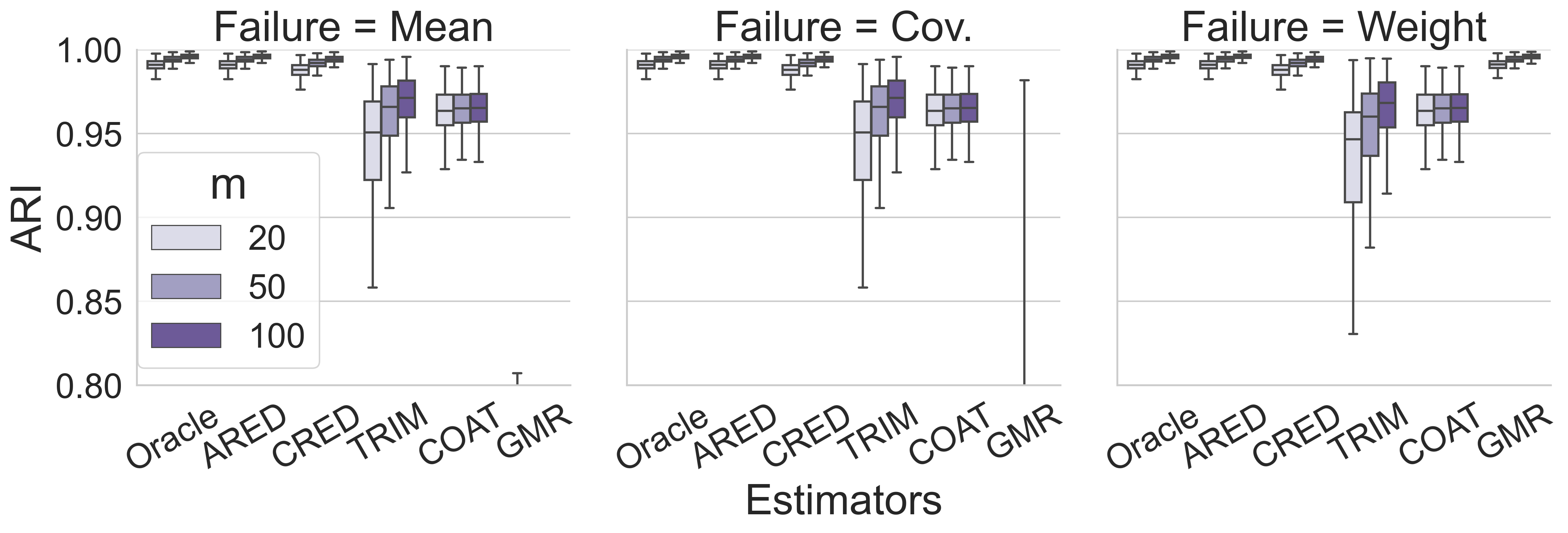
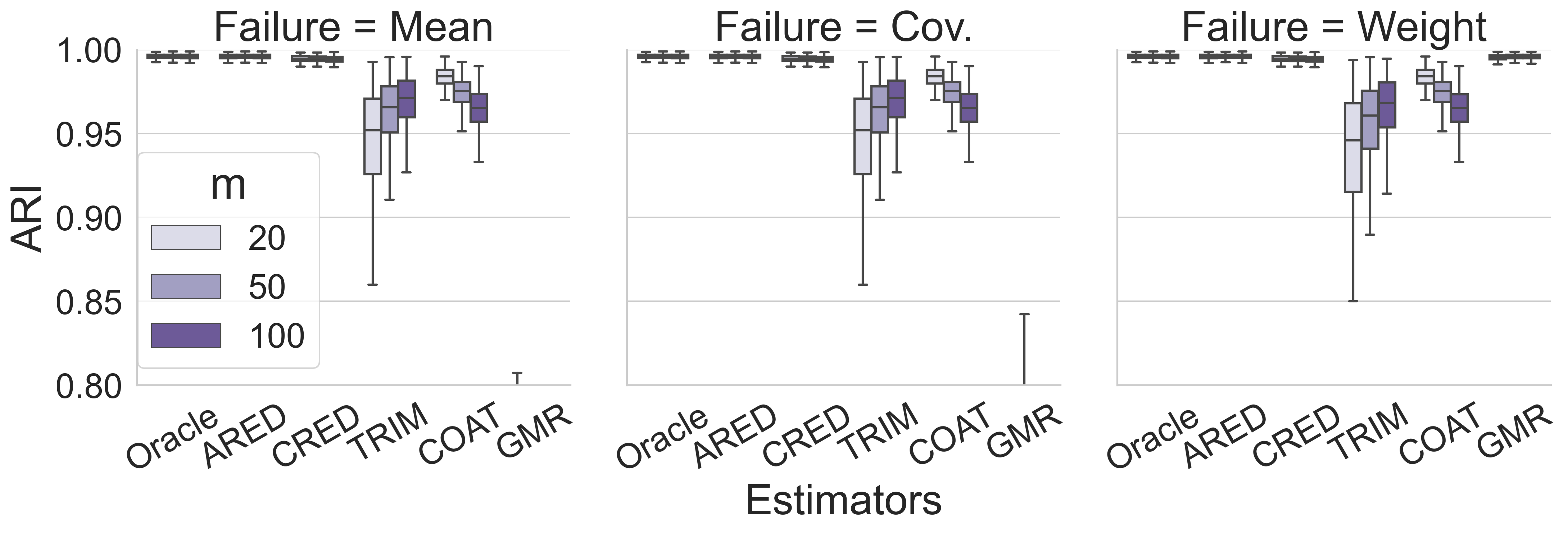
Figure 10 corresponds to the settings in Figure 5. The y-axis is constrained to $[0.5,1.0]$ toemphasize the differences among estimators. The GMR estimator under mean attack has a low ARI and is therefore not shown in the first panel.

Figure 10: The ARI of different clustering methods based on the full dataset as the degree of overlap MaxOmega varies, with $\alpha=0.2$, $m=100$, and local sample size $n=5000$, under various failure scenarios.

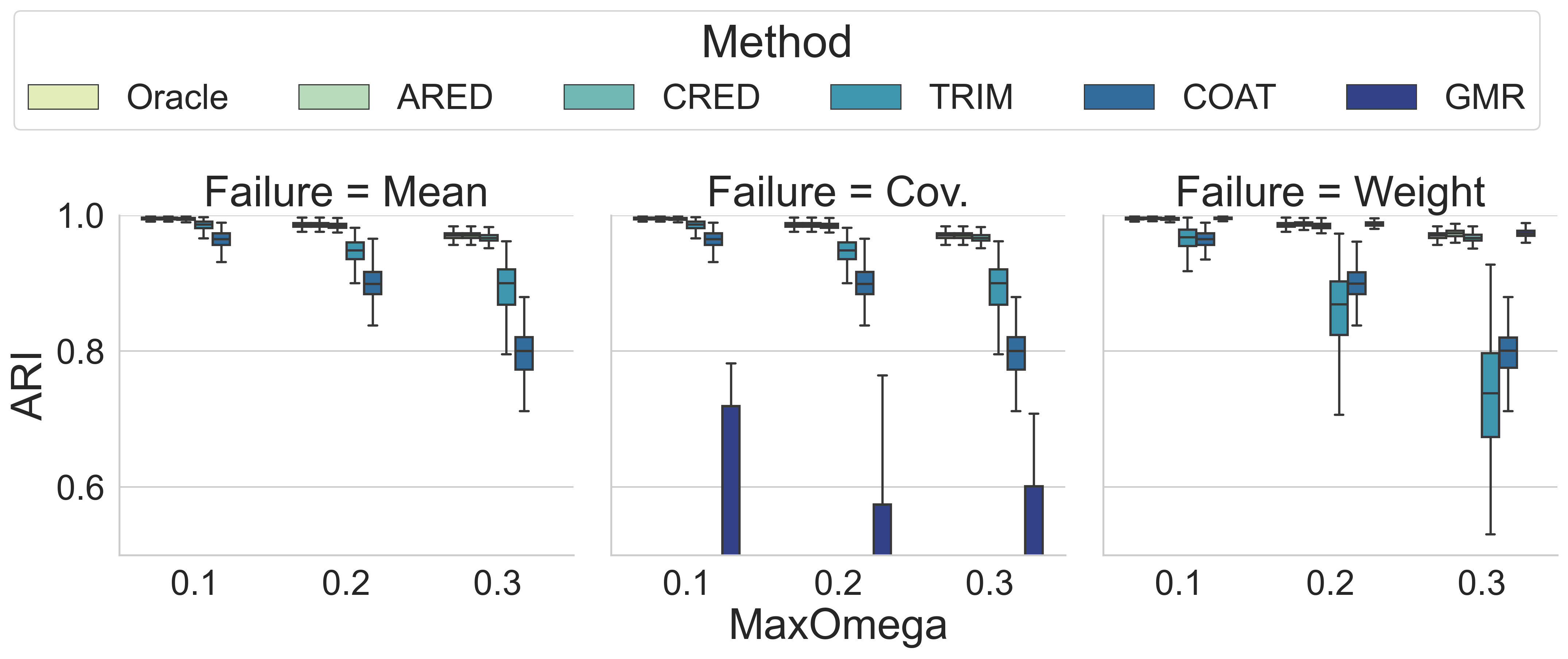
C.3 Real data details

We use the second edition of the NIST dataset. The dataset named by_class.zip is downloaded from https://www.nist.gov/srd/nist-special-database-19. It consists of approximately 4 million images of handwritten digits and letters (0–9, A–Z, and a–z) by different writers. Each digit or letter has its own directory, with the hsf_4 subdirectory designated as the test set, and a train subdirectory containing the training data.

Following common practice, we train a $5$-layer convolutional neural network (CNN) to reduce each image to a $d=50$ feature vector of real values. The CNN architecture used for dimension reduction in the NIST experiment is described in Table 3. The final softmax layer in a CNN can be interpreted as fitting a multinomial logistic regression model on reduced feature space.

Table 3: Architecture and layer specifications of the CNN for dimension reduction in the NIST example. $C_{\text{in}}$, $C_{\text{out}}$, $H$, and $W$ denote the input channel size, output channel size, height, and width of the convolutional kernel, respectively.

Layer	Specification	Activation Function
Conv2d	$C_{\text{in}}=1$, $C_{\text{out}}=20$, $H=W=5$	ReLU
MaxPool2d	$k=2$	–
Conv2d	$C_{\text{in}}=20$, $C_{\text{out}}=50$, $H=W=5$	ReLU
MaxPool2d	$k=2$	–
Flatten	–	–
Linear	$H_{\text{in}}=800$, $H_{\text{out}}=50$	ReLU
Linear	$H_{\text{in}}=50$, $H_{\text{out}}=10$	Softmax

We implemented the CNN in PyTorch 2.2.1 (Paszke et al., 2019) and trained it for $10$ epochs on the NIST training dataset. We used the SGD optimizer with a learning rate of $0.01$, momentum of $0.9$, and a batch size of $64$. After training, we discarded the final layer and employed the resulting CNN to reduce the dimension to $50$ for both the training and test sets. These $50$-dimensional numerical features are then utilized to fit Gaussian mixture models on the training set and evaluate performance on the test set.

References

- Alistarh et al. (2018) Alistarh, D., Z. Allen-Zhu, and J. Li (2018). Byzantine stochastic gradient descent. In S. Bengio, H. Wallach, H. Larochelle, K. Grauman, N. Cesa-Bianchi, and R. Garnett (Eds.), Advances in Neural Information Processing Systems, Volume 31. Curran Associates, Inc.
- Balakrishnan et al. (2017) Balakrishnan, S., M. J. Wainwright, and B. Yu (2017). Statistical guarantees for the EM algorithm: From population to sample-based analysis. Annals of Statistics 45(1), 77–120.
- Baldry et al. (2004) Baldry, I. K., M. L. Balogh, R. Bower, K. Glazebrook, and R. C. Nichol (2004). Color bimodality: implications for galaxy evolution. In AIP Conference Proceedings, Volume 743, pp. 106–119. AIP.
- Battey et al. (2018) Battey, H., J. Fan, H. Liu, J. Lu, and Z. Zhu (2018). Distributed testing and estimation under sparse high dimensional models. Annals of statistics 46(3), 1352.
- Baudry et al. (2010) Baudry, J.-P., A. E. Raftery, G. Celeux, K. Lo, and R. Gottardo (2010). Combining mixture components for clustering. Journal of Computational and Graphical Statistics 19(2), 332–353.
- Chang et al. (2017) Chang, X., S.-B. Lin, and Y. Wang (2017). Divide and conquer local average regression. Electronic Journal of Statistics 11(1), 1326–1350.
- Chen (2023) Chen, J. (2023). Statistical Inference Under Mixture Models. Springer Nature.
- Chen et al. (2016) Chen, J., S. Li, and X. Tan (2016). Consistency of the penalized MLE for two-parameter Gamma mixture models. Science China Mathematics 59(12), 2301–2318.
- Chen and Tan (2009) Chen, J. and X. Tan (2009). Inference for multivariate normal mixtures. Journal of Multivariate Analysis 100(7), 1367–1383.
- Chen et al. (2008) Chen, J., X. Tan, and R. Zhang (2008). Inference for normal mixtures in mean and variance. Statistica Sinica 18(2), 443–465.
- Chen et al. (2022) Chen, X., W. Liu, and Y. Zhang (2022). First-order newton-type estimator for distributed estimation and inference. Journal of the American Statistical Association 117(540), 1858–1874.
- Chen and Xie (2014) Chen, X. and M. Xie (2014). A split-and-conquer approach for analysis of extraordinarily large data. Statistica Sinica 24(4), 1655–1684.
- Chen et al. (2019) Chen, Y., T. T. Georgiou, and A. Tannenbaum (2019). Optimal transport for Gaussian mixture models. IEEE Access 7, 6269–6278.
- Chen et al. (2017) Chen, Y., L. Su, and J. Xu (2017). Distributed statistical machine learning in adversarial settings: Byzantine gradient descent. Proceedings of the ACM on Measurement and Analysis of Computing Systems 1(2), 1–25.
- Crouse et al. (2011) Crouse, D. F., P. Willett, K. Pattipati, and L. Svensson (2011). A look at Gaussian mixture reduction algorithms. In 14th International Conference on Information Fusion, pp. 1–8. IEEE.
- Del Barrio et al. (2019) Del Barrio, E., J. A. Cuesta-Albertos, C. Matrán, and A. Mayo-Íscar (2019). Robust clustering tools based on optimal transportation. Statistics and Computing 29, 139–160.
- Delon and Desolneux (2020) Delon, J. and A. Desolneux (2020). A Wasserstein-type distance in the space of Gaussian mixture models. SIAM Journal on Imaging Sciences 13(2), 936–970.
- Fan et al. (2023) Fan, J., Y. Guo, and K. Wang (2023). Communication-efficient accurate statistical estimation. Journal of the American Statistical Association 118(542), 1000–1010.
- Fan et al. (2019) Fan, J., D. Wang, K. Wang, and Z. Zhu (2019). Distributed estimation of principal eigenspaces. Annals of Statistics 47(6), 3009–3031.
- Feng et al. (2015) Feng, J., H. Xu, and S. Mannor (2015). Distributed robust learning.
- Fraley and Raftery (2002) Fraley, C. and A. E. Raftery (2002). Model-based clustering, discriminant analysis, and density estimation. Journal of the American Statistical Association 97(458), 611–631.
- Ge et al. (2015) Ge, H., Y. Chen, M. Wan, and Z. Ghahramani (2015). Distributed inference for Dirichlet process mixture models. In International Conference on Machine Learning, pp. 2276–2284. PMLR.
- Grother and Hanaoka (2016) Grother, P. and K. Hanaoka (2016). NIST special database 19 handprinted forms and characters 2nd edition. Technical report, National Institute of Standards and Technology.
- Gu (2008) Gu, D. (2008). Distributed EM algorithm for Gaussian mixtures in sensor networks. IEEE Transactions on Neural Networks 19(7), 1154–1166.
- Hathaway (1985) Hathaway, R. J. (1985). A constrained formulation of maximum-likelihood estimation for normal mixture distributions. Annals of Statistics 13(2), 795–800.
- Jordan et al. (2019) Jordan, M. I., J. D. Lee, and Y. Yang (2019). Communication-efficient distributed statistical inference. Journal of the American Statistical Association 114(526), 668–681.
- Lamport et al. (1982) Lamport, L., R. Shostak, and M. Pease (1982). The Byzantine generals problem. ACM Transactions on Programming Languages and Systems 4(3), 382–401.
- Lee et al. (2017) Lee, J. D., Q. Liu, Y. Sun, and J. E. Taylor (2017). Communication-efficient sparse regression. Journal of Machine Learning Research 18(1), 115–144.
- Li et al. (2013) Li, R., D. K. Lin, and B. Li (2013). Statistical inference in massive data sets. Applied Stochastic Models in Business and Industry 29(5), 399–409.
- Liesenfeld (2001) Liesenfeld, R. (2001). A generalized bivariate mixture model for stock price volatility and trading volume. Journal of Econometrics 104(1), 141–178.
- Liu and Rubin (1994) Liu, C. and D. B. Rubin (1994). The ECME algorithm: a simple extension of EM and ECM with faster monotone convergence. Biometrika 81(4), 633–648.
- Liu and Ihler (2014) Liu, Q. and A. T. Ihler (2014). Distributed estimation, information loss and exponential families. In Z. Ghahramani, M. Welling, C. Cortes, N. Lawrence, and K. Weinberger (Eds.), Advances in Neural Information Processing Systems, Volume 27. Curran Associates, Inc.
- Lucic et al. (2017) Lucic, M., M. Faulkner, A. Krause, and D. Feldman (2017). Training Gaussian mixture models at scale via coresets. Journal of Machine Learning Research 18(1), 5885–5909.
- Marín et al. (2005) Marín, J. M., M. Rodriguez-Bernal, and M. P. Wiper (2005). Using Weibull mixture distributions to model heterogeneous survival data. Communications in Statistics–Simulation and Computation 34(3), 673–684.
- Meilijson (1989) Meilijson, I. (1989). A fast improvement to the EM algorithm on its own terms. Journal of the Royal Statistical Society: Series B (Statistical Methodology) 51(1), 127–138.
- Melnykov et al. (2012) Melnykov, V., W.-C. Chen, and R. Maitra (2012). MixSim: an R package for simulating data to study performance of clustering algorithms. Journal of Statistical Software 51(12), 1–25.
- Meng and Rubin (1993) Meng, X.-L. and D. B. Rubin (1993). Maximum likelihood estimation via the ECM algorithm: a general framework. Biometrika 80(2), 267–278.
- Minsker (2019) Minsker, S. (2019). Distributed statistical estimation and rates of convergence in normal approximation. Electronic Journal of Statistics 13(2), 5213–5252.
- Nissim et al. (2007) Nissim, K., S. Raskhodnikova, and A. Smith (2007). Smooth sensitivity and sampling in private data analysis. In Proceedings of the thirty-ninth annual ACM symposium on Theory of computing, pp. 75–84.
- Nowak (2003) Nowak, R. D. (2003). Distributed EM algorithms for density estimation and clustering in sensor networks. IEEE Transactions on Signal Processing 51(8), 2245–2253.
- Paszke et al. (2019) Paszke, A., S. Gross, F. Massa, A. Lerer, J. Bradbury, G. Chanan, T. Killeen, Z. Lin, N. Gimelshein, L. Antiga, A. Desmaison, A. Kopf, E. Yang, Z. DeVito, M. Raison, A. Tejani, S. Chilamkurthy, B. Steiner, L. Fang, J. Bai, and S. Chintala (2019). Pytorch: An imperative style, high-performance deep learning library. In H. Wallach, H. Larochelle, A. Beygelzimer, F. d'Alché-Buc, E. Fox, and R. Garnett (Eds.), Advances in Neural Information Processing Systems, Volume 32. Curran Associates, Inc.
- Pearson (1894) Pearson, K. (1894). Contributions to the mathematical theory of evolution. Philosophical Transactions of the Royal Society of London. A 185, 71–110.
- Ridolfi and Idier (2001) Ridolfi, A. and J. Idier (2001). Penalized maximum likelihood estimation for univariate normal mixture distributions. In AIP Conference Proceedings, Volume 568, pp. 229–237. AIP.
- Salimans et al. (2016) Salimans, T., A. Karpathy, X. Chen, and D. P. Kingma (2016). PixelCNN++: Improving the PixelCNN with discretized Logistic mixture likelihood and other modifications. In International Conference on Learning Representations.
- Tian et al. (2024) Tian, Y., H. Weng, and Y. Feng (2024). Towards the theory of unsupervised federated learning: Non-asymptotic analysis of federated EM algorithms.
- Tu et al. (2021) Tu, J., W. Liu, X. Mao, and X. Chen (2021). Variance reduced median-of-means estimator for Byzantine-robust distributed inference. Journal of Machine Learning Research 22(84), 1–67.
- Vershynin (2018) Vershynin, R. (2018). High-dimensional probability: An introduction with applications in data science, Volume 47. Cambridge university press.
- Wang et al. (2024) Wang, Q., J. Du, and Y. Sheng (2024). Distributed empirical likelihood inference with or without byzantine failures.
- Wu (1983) Wu, C. J. (1983). On the convergence properties of the EM algorithm. Annals of Statistics 11(1), 95–103.
- Wu et al. (2023) Wu, S., D. Huang, and H. Wang (2023). Quasi-Newton updating for large-scale distributed learning. Journal of the Royal Statistical Society: Series B (Statistical Methodology) 85(4), 1326–1354.
- Xie et al. (2018) Xie, C., O. Koyejo, and I. Gupta (2018). Generalized Byzantine-tolerant SGD.
- Yin et al. (2018) Yin, D., Y. Chen, R. Kannan, and P. Bartlett (2018). Byzantine-robust distributed learning: Towards optimal statistical rates. In International Conference on Machine Learning, pp. 5650–5659. PMLR.
- Yin et al. (2019) Yin, D., Y. Chen, R. Kannan, and P. Bartlett (2019). Defending against saddle point attack in byzantine-robust distributed learning. In International Conference on Machine Learning, pp. 7074–7084. PMLR.
- Zhang and Chen (2022) Zhang, Q. and J. Chen (2022). Distributed learning of finite Gaussian mixtures. Journal of Machine Learning Research 23(1), 4265–4304.
- Zhang et al. (2015) Zhang, Y., J. Duchi, and M. Wainwright (2015). Divide and conquer kernel ridge regression: A distributed algorithm with minimax optimal rates. Journal of Machine Learning Research 16(1), 3299–3340.