Double Gradient Reversal Network for Single-Source Domain Generalization in Multi-mode Fault Diagnosis

Abstract

Domain generalization achieves fault diagnosis on unseen modes. In process industrial systems, fault samples are limited, and only single-mode fault data can be obtained. Extracting domain-invariant fault features from single-mode data for unseen mode fault diagnosis poses challenges. Existing methods utilize a generator module to simulate samples of unseen modes. However, multi-mode samples contain complex spatiotemporal information, which brings significant difficulties to accurate sample generation. Therefore, double gradient reversal network (DGRN) is proposed. First, the model is pre-trained to acquire fault knowledge from the single seen mode. Then, pseudo-fault feature generation strategy is designed by Adaptive instance normalization, to simulate fault features of unseen mode. The dual adversarial training strategy is created to enhance the diversity of pseudo-fault features, which models unseen modes with significant distribution differences. Subsequently, domain-invariant feature extraction strategy is constructed by contrastive learning and adversarial learning. This strategy extracts common features of faults and helps multi-mode fault diagnosis. Finally, the experiments were conducted on Tennessee Eastman process and continuous stirred-tank reactor. The experiments demonstrate that DGRN achieves high classification accuracy on unseen modes while maintaining a small model size.

[a]organization=School of Automation,addressline=Wuhan University of Technology, city=Wuhan, postcode=430070, country=PR China [b]organization=The School of Information Technology,addressline=Halmstad University, city=Halmstad, country=Sweden

1 Introduction

Modern process systems are highly automated and intelligent, resulting in substantial increases in scale and complexity [1]. Within the plant system, the coupling of equipment is strong. Fault of a single equipment can cause a series of equipment faults through internal propagation, or even lead to a loss of control of the system. Faulty events have significant economic, safety and environmental impact [2]. The type, location, magnitude, and time of the fault can be determined by fault diagnosis model [3]. Therefore, fault diagnosis plays an important role in ensuring the safe and reliable operation of process systems [4].

Data-driven fault diagnosis methods have gained widespread attention due to their high accuracy and low requirement for specialized knowledge [5, 6]. Data-based methods can be divided into multivariate statistical analysis based and machine learning based methods. Multivariate statistical analysis based methods have been successfully applied to industrial systems, such as principal component analysis (PCA), independent component analysis (ICA), partial least squares (PLS) and Fisher’s discriminant analysis [7, 8, 9, 10]. This kind of methods usually have specific assumptions, which makes them not applicable to all situations. Among methods based on machine learning, k-nearest neighbors (KNN), support vector machine (SVM), random forest (RF) and Bayesian network (BN) have been successfully applied [11, 12, 13, 14, 15]. Lou et al. proposed statistical subspaces to deal with unseen faults [16]. Deng et al. proposed a fault detection method based on space-time compressed matrix and naive Bayes, which can significantly reduce learning complexity while ensuring classification performance [17]. These methods are limited in processing high-dimensional data, and the performance depends on the quality of feature engineering.

Compared with traditional machine learning methods, deep learning based methods can automatically extract features and achieve high accuracy [18]. Convolutional neural network (CNN), deep belief network (DBN), stacked autoencoders (SAE), long short-term memory network (LSTM), and vision transformer (ViT) have been successfully applied to solve the fault diagnosis problems in process industry systems [19, 20, 21, 22, 23, 24]. Hashim et al. combines a multi-Gaussian assumption and an attribute fusion network to enhance zero-shot fault diagnosis [25]. Huang et al. considered time delay of fault occurrence and proposed the CNN-LSTM model [26]. Zhang et al. developed a maximum smooth function (MSF) to replace the classical activation function and proposed a gated recurrent unit-enhanced deep convolutional neural network model [27]. Wei et al. introduced target-attention in the decoder of the transformer [28]. This method enhanced the ability to capture long-term dependencies and detect faults early.

Deep learning based methods [29] assume that the training set and the test set obey the same data distribution. The operating points of industrial systems vary with the environment, loads and production requirements, resulting in differences in the data distribution between the training and test sets [30]. Transfer learning aims to extract the knowledge from one or more source tasks and applies the knowledge to a target task, which can solve the problem of changes in data distribution [31]. For labeled and unlabeled fault data of target mode, Wu et al. proposed fine-tuning and joint adaptive network methods to build a fault diagnosis model [32]. Wang et al. used linear discriminant analysis (LDA) to assign weights to each feature variable and designed a weighted maximum mean discrepancy (MMD) for domain adaptation [33]. Gao et al. used class prior distribution adaptation to generate class-specific auxiliary weights. This method can exploit the prior probability on the source and target domains [34]. Chai et al. suggested to learn features through multi-domain discriminators competition. This method achieved global alignment of two domains and fine-grained alignment of each fault class [35]. Transfer learning based methods require both labeled source domain data and unlabeled target domain data. However, the target domain data is usually unavailable in real systems.

Domain generalization intends to learn a model from one or several domains that can be generalized to unseen domains [36]. Domain generalization based methods have been successfully applied in fault diagnosis. Xiao et al. proposed to align the label distribution by weighting the source classification loss, and to learn domain-invariant feature representations by progressive adversarial training [37]. Huang et al. constructed causal layers to discover causal mechanism in features and developed a domain classifier cooperating with gradient reversal layers to capture the domain invariance [38]. Xiao et al. proposed a method to learn a classifier and invariant feature representation simultaneously based on the weighted variables [39]. Domain generalization based methods learn fault knowledge in multi-mode that can be generalized to unseen modes. However, it’s difficult to obtain fault data for multiple conditions. Fault data is only available for a single mode.

In single-source domain generalization for multi-mode fault diagnosis, a common approach is to first generate unseen mode samples from source domain samples, then construct a fault diagnosis model using both source and generated samples. Zhao et al. proposed an adversarial mutual information-guided single domain generalization network (AMINet) [40]. This method designs an iterative min–max game of mutual information between the domain generation module and task diagnosis module to learn generalized features. Wang et al. designed an adversarial contrastive learning strategy, which can promote the learning of class-wise domain-invariant representations while maintaining the diversity of the generated samples [41]. Pu et al. presented an incremental domain augmentation strategy. This method can generate several augmented domains with different distributions but the same semantic information [42]. Guo et al. used Mixup to create augmented domains with significant distributional differences from the source domain [43]. However, the data collected from industrial systems contain complex spatial-temporal information, accurately generating samples of unknown modes is challenging. Additionally, most methods use classifiers as arbiters to determine the fault class of the generated samples. This can lead to erroneous samples being generated by the generator before the classifier has fully learned the true classification criteria.

To address the above problems, this paper proposes a novel network architecture, the double gradient reversal network (DGRN). The DGRN is pre-trained to learn the fault features from single seen mode. Adaptive instance normalization (AdaIN) is employed to generate pseudo-fault features based on fault features extracted from single seen mode. The Supervised learning ensures that pseudo-fault features retain the semantic information of the fault. The dual adversarial training strategy is created to increase the diversity of pseudo-fault features. By integrating adversarial and supervised contrastive learning, DGRN extracts domain-invariant fault features from both pseudo-fault features and the single seen mode fault features, addressing the challenge of mutli-mode fault diagnosis.

The main contributions of this paper are as follows: (1) DGRN is proposed to solve the problem of single-domain generalization in multi-mode fault diagnosis. The model can be trained from a single mode of fault data and generalized to multiple unseen modes. (2) Pseudo-fault feature generation strategy is designed using AdaIN, which models the fault features of unseen mode. The dual adversarial training strategy, implemented by two gradient reversal layers, enhances the diversity of pseudo-fault features. (3) Domain-invariant feature extraction strategy is established by merging contrastive learning with adversarial learning, enabling the extraction of common fault features from both single seen mode fault features and pseudo-fault features. (4) The effectiveness of DGRN is validated through extensive experiments on the Tennessee Eastman process and the Continuous Stirred-Tank Reactor (CSTR). The results indicate that DGRN not only achieves robust generalization but also maintains a compact model size.

2 Preliminaries

2.1 Problem formulation

The operational modes of process industry systems are constantly changing, leading to variations in the data distribution of monitored variables. However, fault data for multi-mode is difficult to obtain, and typically, only single-mode fault data is available. Single-domain generalization in multi-mode fault diagnosis refers to constructing a model using fault data from a single mode, which exhibits strong generalization capabilities to other unseen modes.

Assume that ${{N}_{\text{S}}}$ labeled fault samples $D_{\mathrm{S}}=\{x_{i},y_{i}\},i=1,...,N_{\mathrm{S}}$ in one mode is available and can be used to train a fault diagnosis model. The training goal for the single source domain generalization based fault diagnosis model is to achieve a high fault diagnosis accuracy in the sample sets of other $m$ unseen modes $D_{\mathrm{T}}=\{D_{\mathrm{t1}},...,D_{\mathrm{tm}}\}$. $D_{\mathrm{S}}$ and $D_{\mathrm{T}}$ are referred to as the source domain and target domain, respectively. They share the same feature space and label space.

2.2 Motivation

The objective of this study is to develop a model that demonstrates robust generalization performance on various unseen modes, utilising data obtained from a single mode. In the field of image style transfer, images of a specific style contain content and style information [44]. Similarly, the fault data for a specific mode can be viewed as a combination of fault features and mode features. When the system operates stably in one mode, it can be regarded as a wide-sense stationary process. A wide-sense stationary process can be described by its mean and autocorrelation function. Assume the mode features in the monitoring data are described by the mean of each variable under normal condition. Standarizing each variable by subtracting the mean and dividing by the standard deviation removes mode features and scales variables to the same level. The standardized data contains only fault features, which represents the system’s health condition.

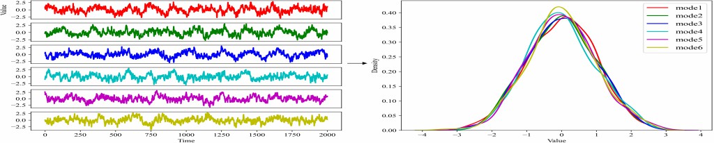
(a) Normal data.

(b) Fault 2 data.

(c) Normal and fault 2 data of material A flow rate after standardization of the Tennessee Eastman process in six modes.

Fig. 1 shows the normal data and fault 2 data of material A flow rate after standardization of the Tennessee Eastman process in six modes, respectively. The left shows the curve of the variable over time, and the right represents the probability density function of the variable. It can be seen that the distribution difference of normal data after standardization can be ignored, while the distribution difference of fault 2 data still exists. The features contained in the standardized fault data can be divided into domain-invariant and domain-specific fault features. Domain-invariant fault features remain consistent across different modes. For example, the specific monitored variables affected by a fault and the trends in these variable changes can be considered domain-invariant fault features. Domain -specific fault features vary with modes, such as change amplitude of a monitored variables affected by faults. As can be seen from Fig. 1, the data distribution of material A flow rate shifts in the positive direction, which can be regarded as a domain-invariant feature of the fault 2. And the magnitude of the increase in the flow rate of material A or the specific details of the change can be regarded as a domain-specific feature of fault 2. Both domain-invariant and domain-specific fault features can distinguish the fault class under a certain mode. The key to single-domain generalization in multi-mode fault diagnosis is to extract domain-invariant fault features of the faults.

With the aim of generalizing the fault diagnosis model constructed on single-mode dataset to other modes, a feasible idea is to generate diverse samples, which should cover faults sample space of unseen modes as much as possible. From this perspective, the generalization performance of the fault diagnosis model can be limited by the generated fault data. However, directly generating samples of unseen modes is complex. Therefore, generating samples of unseen modes is transformed into generating pseudo-fault features. Additionally, in the process of generating pseudo-fault features, how to retain domain-invariant fault features while increasing diversity needs to be focused on.

2.3 Diversity of generated samples

The purpose of increasing sample diversity is to ensure that the generated samples cover as much of the unseen mode sample space as possible, thereby enhancing the completeness of the training samples. The upper bound of mutual information was minimized to encourage diversity distributions in [40]. The multi-scale style generation strategy and adversarial contrastive learning strategy are adopted to enable the generated samples more diverse in [41]. An incremental domain augmentation strategy is proposed to generate augmented domains with difference and completeness in [42]. Multi-scale deep separable convolutional kernels and mixup are combined to generate extended domain samples with different distributions in [43]. These methods achieve the generation of diverse samples. During the sample generation process, domain-invariant fault features remain unchanged. Therefore, sample generation should be constrained by domain-invariant fault features.

2.4 Domain-invariant feature extraction

Domain-invariant fault features do not change with different modes. Therefore, in multi-mode fault diagnosis, extracting domain-invariant fault features helps diagnose fault classes. Lower bound of mutual information was maximized to learn sematic-consistent representations in [40]. Contrastive learning is used tolearn class-wise domain-invariant representations in [41, 42]. Adversarial training and metric learning strategy is designed to learn generalized features in [43]. For samples with strong diversity, supervised contrastive learning and adversarial learning alone may not be able to learn domain-invariant fault features well. Therefore, different strategies need to be combined to enhance the learning of domain-invariant fault features.

3 Proposed method

3.1 Overall structure of DGRN

DGRN is trained with samples from single seen mode and tested with samples from unseen modes. The overall structure of DGRN is shown in Fig. 2. Both pre-training process and training-process are based on a single-mode samples for training. After the pre-training process, DGRN would learn the fault knowledge of the single seen mode. Then during the training process, DGRN would generate diverse pseudo-fault features based on seen mode fault knowledge, extract domain-invariant fault features, and then diagnose fault classes. After these two processes, DGRN is well-trained. DGRN consists of data processing, feature extractor $F$, AdaIN feature transformer $H$, domain invariant feature extractor $G$, classifier $C$ and discriminator $D$. The detailed composition of each module is shown in Table 1, where $v$ is the number of monitored variables.

Table 1: Structure of the modules in DGRN.

Modules	Type	(Input size, output size, kernel size)
Feature extractor	Conv1d	($v$×64, 128×64, $v$×3)
	Max pooling	(128×64, 128×32, -)
	Conv1d	(128×32, 128×32, 128×3)
	Max pooling	(128×32, 128×16, -)
	Conv1d	(128×16, 128×16, 128×3)
AdaIN feature transformer	-	(128×16, 128×16, -)
Domain invariant feature extractor	Fully connected	(2048,256, -)
Classifier	Fully connected	(256, c, -)
Discriminator	Fully connected	((256×c), 1, -)

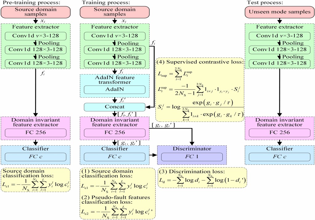
Fig. 1.: Overall structure of DGRN.

3.1.1 Data processing

Data processing mainly consists of standardization and time series expansion. As mentioned in section 2.2, it is assumed that the mode features can be represented by the mean and variance the fault-free data. Thus, standardization is performed to remove mode features in the data. Temporal fault data contains rich spatiotemporal feature information. Time series expansion is employed to preserve the temporal features of the data. Time series expansion is implemented by expanding the data of the previous $k-1$ moments to the current moment.

3.1.2 Feature extractor

Feature extractor $F$ takes the samples after data processing as inputs and outputs deep-level features. It maps the sample space to the feature space using three 1-dimensional convolutional layers and two max-pooling layers. ReLU is used as the activation function [45]. The activation function is located after each maximum pooling layer and the last 1-dimensional convolutional layer. Let $f_{i}$ denotes the fault features of sample $x_{i}$, $f_{i}=F\left(x_{i}\right)$.

3.1.3 AdaIN feature transformer

The deep-level features extracted by feature extractor contains domain-invariant and domain-specific fault features. From Fig. 1, it can be seen that the change trend and change amplitude of the fault-related variables can be regarded as domain-invariant and domain-specific fault features, respectively. Therefore, unseen mode fault features can be simulated by varying the magnitude of single seen mode fault features. AdaIN feature transformer $H$ generates pseudo-fault features $f_{i}’$ based on the single seen mode fault features $f_{i}$. $f_{i}’=H\left(f_{i},n_{1},n_{2}\right)={h_{1}\left(n_{1}\right)\left(f_{i}-\mu_{i}\right)}/{\sigma_{i}}+h_{2}\left(n_{2}\right)$, where $n_{1}$ is randomly sampled from a uniform distribution between 0.05 and 1.95, $n_{2}$ is random sampled from standard Gaussian distribution, $h_{1}$ and $h_{2}$ are fully connected layers, $\mu_{i}$ and $\sigma_{i}$ is the mean and variance of $f_{i}$. $h_{1}\left(n_{1}\right)$ and $h_{2}\left(n_{2}\right)$ are used to simulate the variations in fault feature magnitude and steady-state noise.

Concat is the module to splice single seen mode fault features and pseudo-fault features in the batch dimension.

3.1.4 Domain-invariant feature extractor

Both single seen mode fault features and pseudo-fault features contain domain-invariant and domain-specific fault features. And only domain invariant fault features contribute to multi-mode fault diagnosis. The domain-invariant feature extractor $G$ is expected to implement the function of extracting domain-invariant fault features from single seen mode fault features and pseudo-fault features through a fully connected layer. The activation function is ReLU, and dropout is added to avoid overfitting. Let $g_{i}$ and $g_{i}^{\prime}$ denote the domain-invariant fault features of single seen mode data and pseudo-fault data, respectively. $g_{i}$ and $g_{i}^{\prime}$ are defined as, $\begin{bmatrix}g_{i},g_{i}^{\prime}\end{bmatrix}=G(\begin{bmatrix}f_{i},f_{i}^{\prime}\end{bmatrix})$.

3.1.5 Classifier

The classifier $C$ takes the extracted domain-invariant fault features as inputs and outputs the fault class. It is also implemented through a fully connected layer. Let $c_{i}$ and $c_{i}^{\prime}$ denote the classifier predictions of single seen mode data and pseudo-fault data, respectively. $c_{i}$ and $c_{i}^{\prime}$ are defined as, $\begin{bmatrix}c_{i},c_{i}^{\prime}\end{bmatrix}=C(\begin{bmatrix}g_{i},g_{i}^{\prime}\end{bmatrix})$.

3.1.6 Discriminator

Mode classes are distinguished by Discriminator $D$. In multi-mode fault diagnosis, fault data exhibits multi-modal structural characteristics. Long et al. proposed that the multimodal structures can only be captured sufficiently by the cross-covariance dependency between the features and classes [46]. Thus, the discriminator is conditioned on the cross-covariance of domain-invariant feature representations and classifier predictions. The discriminator predictions of single seen mode data and pseudo-fault data are defined as, $\begin{bmatrix}d_{i},d^{\prime}_{i}\end{bmatrix}=D\left(\begin{bmatrix}g_{i},g^{\prime}_{i}\end{bmatrix}\otimes\begin{bmatrix}c_{i},c^{\prime}_{i}\end{bmatrix}\right)$, where $\otimes$ is a multilinear mapping.

3.2 Pre-training process

The pre-training process enables the DGRN model to learn single seen mode fault features in advance, facilitating the generation of more effective pseudo-fault features during later training process. The fault diagnosis model is established on the single seen mode fault data. Thus, it should first have high classification accuracy on this data set. The fault diagnosis model is optimized through cross-entropy loss of single seen mode data, which is defined as,

$$L_{\mathrm{c}1}=-\frac{1}{N_{\mathrm{s}}}\sum_{i=1}^{N_{\mathrm{s}}}\sum_{l=1}^{L}y_{i}^{l}\log c_{i}^{l}$$ (1)

where $y_{i}^{l}$ is the $l$-th dimension of the true label of the $i$-th sample, and $c_{i}^{l}$ is the $l$-th dimension of the classifier prediction of the $i$-th sample.

3.3 Training process

During training process, DGRN should accurately classify single seen mode samples and ensure pseudo-faults have sufficient semantic information and diversity, enabling domain-invariant feature extraction. To ensure the accurate classification of single seen mode samples, Eq. (1) is used to optimize the fault diagnosis performance of the model.

3.3.1 Semantic preservation of pseudo-fault features

The single seen mode fault features and pseudo-fault features serve as the inputs and outputs of the AdaIN feature transformer, respectively. They possess different domain-specific fault features, while the fault classes remain the same. The fault class labels of the single seen mode data are assigned to the corresponding pseudo-fault features. The label classification loss for the pseudo-fault features is defined as,

$$L_{\mathrm{c}2}=-\frac{1}{N_{\mathrm{s}}}\sum_{i=1}^{N_{\mathrm{s}}}\sum_{l=1}^{L}y_{i}^{l}\log{{c^{\prime}}_{i}^{l}}$$ (2)

where ${c_{i}^{l}}^{\prime}$ is the $l$-th dimension of the classifier prediction of the $i$-th pseudo-fault features.

3.3.2 Domain invariant feature extraction

Fault features extracted from single mode fault data are difficult to discern whether they are domain-invariant or domain-specific fault features. Domain-invariant fault features need to be extracted from multi-mode fault data. Pseudo-fault features represent the fault features of unseen modes. Thus, domain-invariant fault features can be extracted from single seen mode fault features and pseudo-fault features.

Supervised contrastive learning can bring samples belonging to the same class closer in the embedding space while separating samples from different classes [47]. It is used here to pull together samples belonging to the same class in the embedding space. The supervised contrastive loss is defined as,

$$L_{\mathrm{sup}}=\sum_{i=1}^{2N_{\mathrm{s}}}L_{i}^{\mathrm{sup}},L_{i}^{\sup}=\frac{-1}{2N_{\mathrm{S}}-1}\sum_{j=1}^{2N_{\mathrm{S}}}1_{i\neq j}\cdot 1_{y_{i}=y_{j}}\cdot\log\frac{\exp\left(g_{i}\cdot g_{j}/\tau\right)}{\sum\limits_{k=1}^{2N_{\mathrm{s}}}1_{i\neq k}\cdot\exp\left(g_{i}\cdot g_{k}/\tau\right)}$$ (3)

where $1_{A}$ is an indicator function, which means it is 1 when $A$ is satisfied, otherwise it is 0. $\tau$ is a scalar temperature parameter. Since the single seen mode fault features $g$ and pseudo fault features $g’$ are mixed together, they are uniformly recorded as $g$ in Eq. (3).

Domain-invariant fault features may not be effectively extracted using only supervised contrastive learning, especially between samples with significant domain differences. Therefore, adversarial learning is introduced to enhance the representation of domain-invariant fault features. In adversarial learning, domain-invariant fault features are extracted through adversarial training of domain-invariant feature extractor $G$ and discriminator $d$. Maximizing and minimizing the discriminative loss are the optimization objectives for the feature extractor and discriminator, respectively. The discriminative loss is defined as,

$$L_{\mathrm{d}}=-\sum_{i=1}^{N_{\mathrm{S}}}\log d_{i}-\sum_{i=1}^{N_{\mathrm{S}}}\log\left(1-d_{i}^{\prime}\right)$$ (4)

The gradient reversal layer(GRL) between domain-invariant feature extractor and discriminator implements adversarial training, as shown in Fig. 3. The adversarial training is described as follows: Assume that the fault features extracted by the domain invariant feature extractor is divided into domain-invariant fault features and domain-specific fault features. Domain-invariant fault features can be used to identify fault class, but not domain (mode) class. While domain-specific fault features can be taken to determine both fault class and domain (mode) class.

The mode class of the sample is identified by the discriminator, determining whether the current sample belongs to the single seen mode. By minimizing the discriminative loss, discriminator learns the differences in modes as much as possible. Thus, discriminator can be considered as an expert of domain-specific fault features. If domain-specific fault features exist, discriminator can capture them.

The optimization objective of the domain invariant feature extractor is to maximize the discriminative loss. The domain invariant feature extractor reduces the differences between different modes in embedding space. This means that the fault features extracted by the domain-invariant feature extractor cannot contain domain-specific fault features. By the adversarial training, domain-invariant feature extractor and discriminator become experts of domain-invariant and domain-specific fault features, respectively.

3.3.3 Diversity of pseudo-fault features

The analysis in section 3.3.2 shows that the domain-invariant feature extractor can extract domain-invariant fault features, and the discriminator can capture domain-specific fault features. But the premise is that the input of the domain invariant feature extractor is multi-mode fault data.

By maximizing the discriminative loss, the domain-invariant feature extractor can reduce the difference between single seen mode fault features and pseudo-fault features in the embedding space. If the optimization objective of the AdaIN feature transformer is also to maximize the discriminative loss, then the difference between its generated pseudo fault features and the single seen mode fault features will be reduced. The generated pseudo fault features and single seen mode fault features cannot be considered to belong to different modes. This contradicts the premise of section 3.3.2. Thus, the optimization objective of the AdaIN feature transformer is set to minimize the discriminative loss, resulting in a large difference between the generated pseudo-fault features and the single seen mode fault features. There is also a GRL between AdaIN feature transformer and domain-invariant feature extractor, as shown in Fig. 3.

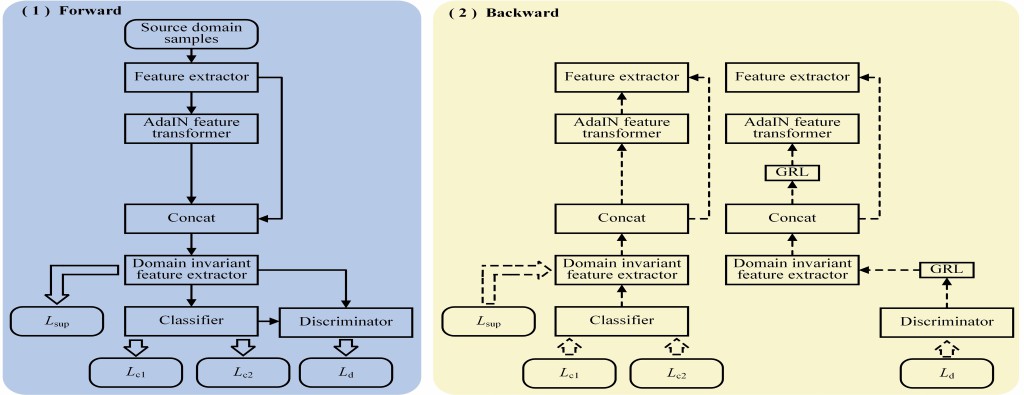
Fig. 2.: Forward and backward propagation of DGRN.

3.3.4 The overall optimization objectives of DGRN

To obtain a unified loss function, the maximization of discriminative loss is converted into the minimization of the negative discriminative loss. The overall loss function used to optimize feature extractor, domain invariant feature extractor and classifier is defined as,

$$L_{1}=L_{\mathrm{c}1}+\lambda_{1}L_{\mathrm{c}2}+\lambda_{2}L_{\sup}-\lambda_{3}L_{\mathrm{d}}$$ (5)

where $\lambda_{1}$, $\lambda_{3}$ and $\lambda_{3}$ are hyperparameters.

The loss function of discriminator is defined as,

$$L_{2}=L_{\mathrm{d}}$$ (6)

The loss function of AdaIN feature transformer is defined as,

$$L_{3}=L_{\mathrm{c}2}+\lambda_{2}L_{\sup}+\lambda_{3}L_{\mathrm{d}}$$ (7)

The training and inference of DGRN is shown in Algorithm 1.

Algorithm 1 DGRN.

# Pre-training stage
Input: Source domain dataset $D_{S}$.
Model: feature extractor $F$, domain invariant feature extractor $G$ and classifier $C$.
Output: feature extractor $F$, domain invariant feature extractor $G$ and classifier $C$.
1: Perform data processing on the source domain dataset
2: for epoch = 1 to epochs do
3:     for batch = 1 to batches do
4:         Calculate classifier output.
5:         Calculate losses $L_{\mathrm{c}1}$ via Eq. (1).
6:         Update parameters of networks through gradient descent algorithm.
7:     end for
8: end for
Return: Pre-trained model.

# Training stage
Input: Source domain dataset $D_{S}$ and pre-trained model.
Model: feature extractor $F$, AdaIN feature transformer $H$, domain invariant feature extractor $G$, classifier $C$ and discriminator $D$.
Output: feature extractor $F$, domain invariant feature extractor $G$, and classifier $C$.
1: Perform data processing on the source domain dataset.
2: Initialize feature extractor $F$, domain invariant feature extractor $G$ and classifier $C$ using parameters obtained from pre-training.
3: for epoch = 1 to epochs do
4:     for batch = 1 to batches do
5:         Calculate classifier and discriminator output.
6:         Calculate the losses $L_{1}$, $L_{2}$ and $L_{3}$ via Eq. (5) to Eq. (7).
7:         Update parameters of networks through gradient descent algorithm.
8:     end for
9: end for
Return: feature extractor $F$, domain invariant feature extractor $G$ and classifier $C$

# Inference stage
Input: Target domain dataset $D_{T}$.
Model: feature extractor $F$, domain invariant feature extractor $G$ and classifier $C$.
Output: Fault class.

4 Experiments

Tennessee Eastman (TE) process [48] and CSTR [49] are used for single-source domain generalization to multi-modes fault diagnosis experiments.

4.1 TE

TE process has become a benchmark for evaluating process monitoring and fault diagnosis models. Its simulation model has been implemented through SIMULINK [50]. LIU et al. obtained models for six modes by adjusting the parameters [51]. The structure of the TE process is shown in Fig. 4. The process consists of 53 monitored variables and can simulate 28 faults in 6 different modes. The fault, mode and task settings used to validate the model are presented in Table 2 - Table 4, respectively.

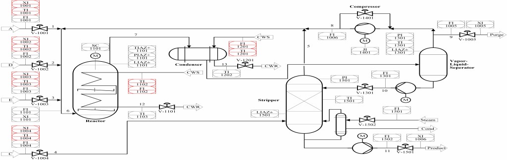
Fig. 3.: P&ID of the revised process model [50].

Table 2: Faults of TE process used in single source domain generalization fault diagnosis [48].

Fault No.	Description	Type
F0	Normal	-
F2	B composition, A/C ratio constant	Step
F4	Reactor cooling water inlet temperature	Step
F8	A, B, C feed composition	Random variation
F10	C feed temperature	Random variation
F11	Reactor cooling water inlet temperature	Random variation
F12	Condenser cooling water inlet temperature	Random variation
F13	Reaction kinetics	Slow drift
F14	Reactor cooling water valve	Sticking
F17	Unknown	-

Table 3: Modes of TE process used in single source domain generalization fault diagnosis [48].

Mode No.	G/H mass ratio	Production rate
M1	50/50	G: 7038kg/h, H: 7038kg/h
M2	10/90	G: 1408kg/h, H: 12669kg/h
M3	90/10	G: 10000kg/h, H: 1111kg/h
M4	50/50	maximum production rate
M5	10/90	maximum production rate
M6	90/10	maximum production rate

Table 4: Single source domain generalization fault diagnosis task description of TE process.

Task No.	Training set (No. of samples: 11200)	Test set 1 (No. of samples: 2810)	Test set 2 (No. of samples: 70050)
T1	M1	M1	M2, M3, M4, M5 and M6
T2	M2	M2	M1, M3, M4, M5 and M6
T3	M3	M3	M1, M2, M4, M5 and M6
T4	M4	M4	M1, M2, M3, M5 and M6
T5	M5	M5	M1, M2, M3, M4 and M6
T6	M6	M6	M1, M2, M3, M4 and M5

In the process of generating datasets through SIMULINK simulation, the sampling interval is set to 3 seconds, and the simulation time is set to 100 hours, with faults implanted starting from 30 hours. Each class will produce 1400 samples in each mode. The length of the time series expansion is set to 64. Data from each mode is sequentially chosen as source domain dataset, and data from the other five modes served as the target domain dataset (test set 2). The source domain dataset is divided into training set and test set 1. The training set and test set 1 are randomly divided, with proportions of 80% and 20%, respectively. The training set is used to build a fault diagnosis model. Test set 1 is used to determine if the model has basic diagnostic capabilities on data distributions similar to the training data. Test set 2, which is the focus of comparison, is used to evaluate the model’s diagnostic performance on unseen modes. By comparing the model’s performance on test set 1 and test set 2, the model learns whether more domain-invariant fault features or domain-specific fault features can be characterized.

4.2 CSTR

Closed-loop CSTR has been also widely used to validate the performance of fault diagnosis algorithms. The monitored variables of the process are shown in Fig. 5. The reactor temperature (T) is controlled by the volumetric flowrate of the cooling water (Q${}_{\mathrm{c}}$).

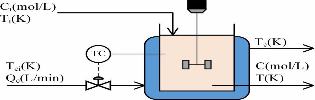
Fig. 4.: Structure of closed-loop CSTR [49].

This process can be described by follows,

$$\frac{dC}{dt}=\frac{Q}{V}\Big{(}C_{i}-C\Big{)}-kC$$ (8)

$$\frac{dT}{dt}=\frac{Q}{V}\Big{(}T_{i}-T\Big{)}-\frac{(\Delta H_{r})kC}{\rho C_{p}}-\frac{UA}{\rho C_{p}V}\Big{(}T-T_{c}\Big{)}$$

$$\frac{dT_{c}}{dt}=\frac{Q_{c}}{V_{c}}\Big{(}T_{ci}-T_{c}\Big{)}+\frac{UA}{\rho_{c}C_{pc}V_{c}}\Big{(}T-T_{c}\Big{)}$$

$$k=k_{0}\exp\biggl{(}\frac{-E}{RT}\biggr{)}$$

where the detailed parameter information can be seen in [49]. The faults set in CSTR are shown in Table 5. Data for mode 1 (M1) were collected at the original set point. Data for mode 2 (M2) and mode 3 (M3) were collected with set points increased by 5K and 10K, respectively. The simulation time was set to 2 hours, with faults introduced at 200 minutes. The division of the dataset followed the same experimental setup as the TE process. Detailed task settings are shown in Table 6.

Table 5: Faults of CSTR used in single source domain generalization fault diagnosis.

Fault No.	Description
F0	Normal
F1	Reactant inlet concentration
F2	Reactant inlet temperature
F3	Coolant inlet temperature
F4	Reactant inlet flow rate
F5	Reactant inlet concentration sensor
F6	Reactant inlet temperature sensor
F7	Reactant outlet temperature sensor
F8	Coolant inlet flow rate sensor
F9	Coolant inlet temperature sensor
F10	Coolant outlet temperature sensor
F11	Catalyst decay
F12	Heat transfer fouling

Table 6: Tasks setting of CSTR used in single source domain generalization fault diagnosis.

Task No.	Training set (No. of samples:10400)	Test set 1 (No. of samples:2613 )	Test set 2 (No. of samples:26026 )
T1	M1	M1	M2,M3
T2	M2	M2	M1,M3
T3	M3	M3	M1,M2

4.3 Comparative models

To validate the effectiveness of the DGRN model, deep convolutional neural network (DCNN), CNN-LSTM, industrial process optimization ViT (IPO-ViT) and multi-scale style generative and adversarial contrastive network(MSG-ACN) are used for comparative tests.

• DCNN [19]. The DCNN model extracts the features in both spatial and temporal domains, consisting of convolutional layers, pooling layers, dropout, and fully connected layers.

• CNN-LSTM [26]. The CNN-LSTM model synthetically considers feature extraction and time delay of occurrence of faults. Feature extraction is achieved through CNN, and temporal delay is captured by LSTM.

• IPO-ViT[23]. The IPO-ViT model is built based on ViT, which utilizes the global receptive field provided by self-attention mechanism. This method can perform global feature learning on the complex process signals.

• MSG-ACN[41]. This method establishes a multi-scale style generation strategy to generate diverse samples. Then domain-invariant fault features are extracted from the source and extended domains via an adversarial contrastive learning strategy. It has been validated a relatively good performance in solving single-domain generalization problems.

• MSG-ACN2. The multi-scale style generation strategy and adversarial contrastive learning strategy in MSG-ACN are applied to pre-trained model. The multi-scale style generation strategy is used to generate pseudo-fault features instead of unseen mode samples there.

4.4 Evaluation metrics

The performance of the fault diagnosis model for class $l$ is measured using accuracy (ACC), fault diagnosis rate (FDR) and false positive rate (FPR), defined as follows,

$$ACC=\frac{\sum_{l=1}^{L}TP_{l}}{\sum_{l=1}^{L}TP_{l}+\sum_{l=1}^{L}FN_{l}}$$ (9)

$$FDR_{l}=\frac{TP_{l}}{TP_{l}+FN_{l}}$$ (10)

$$FPR_{l}=\frac{FP_{l}}{FP_{l}+TN_{l}}$$ (11)

where $TP_{l}$, $FN_{l}$, $FP_{l}$ and $TN_{l}$ are define in the confusion matrix for the $l$-th class, as shown in Table 7.

Table 7: Confusion matrix for the $l$-th class(Number of samples).

	Predicted fault class is $l$	Predicted fault class is not $l$
Actual fault class is $l$	$TP_{l}$	$FN_{l}$
Actual fault class is not $l$	$FP_{l}$	$TN_{l}$

In addition to the above evaluation metrics, the model’s parameter count, training, and testing time are also used to assess model performance.

5 Experimental Results and Analysis

5.1 TE process

5.1.1 Model comparison

DCNN, CNN-LSTM, IPO-ViT, MSG-ACN, MSG-ACN2 and DGRN were tested in the tasks shown in Table 3 respectively. The hyperparameters in MSG-ACN, MSG-ACN2, and DGRN are obtained through Bayesian optimization. For MSG-ACN, the optimization objective is to maximize the classification accuracy of generated samples, while for other models, the objective is to maximize the classification accuracy of pseudo-fault features. Taking T1 as an example, the classification accuracy of DGRN on pseudo-fault features, test set 1 and test set 2 during the Bayesian optimization process are shown in Fig. 6. It can be observed that the classification accuracy of pseudo-fault features reached its highest value of 99.19% in the 57-th optimization iteration. At this point, the classification accuracy on the test set 1 is 98.58%, and on test set 2 it is 93.20%. During the optimization process, the maximum classification accuracies on the two test sets were 98.86% and 94.16%, respectively. This indicates that DGRN has higher diagnostic potential in both the seen mode and unseen modes.

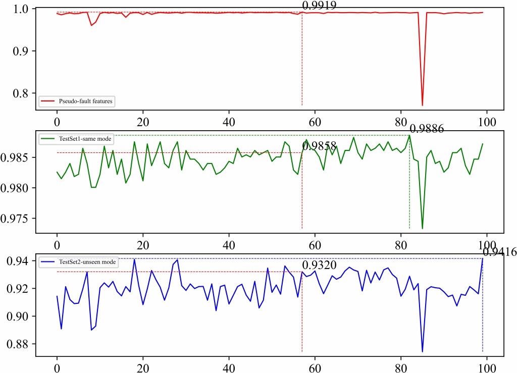
Fig. 5.: Classification accuracy on test set 1, test set 2, and pseudo-fault features during the Bayesian optimization process.

To evaluate whether the model has basic diagnostic capabilities on data distributions similar to the training data, each model is tested on test set 1. The accuracies achieved by each model under different tasks are shown in Table 8. CNN-LSTM obtained the highest average classification accuracy. However, the classification accuracies of CNN-LSTM, MSG-ACN and DGRN are all higher than 99%. This indicates that these three models exhibit high performance in fault diagnosis on single seen mode data.

Table 8: Experimental results on the test set 1 of TE process (Accuracy).

Task No.	DCNN	CNN-LSTM	IPO-ViT	MSG-ACN	MSG-ACN2	DGRN
T1	97.54%	99.07%	97.94%	99.00%	98.22%	98.68%
T2	88.22%	99.40%	97.12%	99.40%	98.83%	99.25%
T3	97.76%	99.50%	98.36%	99.36%	98.33%	99.32%
T4	87.58%	98.97%	96.83%	98.68%	97.37%	98.54%
T5	98.04%	99.40%	97.26%	99.32%	99.07%	99.29%
T6	96.90%	99.32%	98.01%	99.18%	98.43%	99.07%
Avg	94.34%	99.28%	97.59%	99.16%	98.38%	99.03%

The model’s generalization performance on unseen modes is then evaluated. For the test set 2 of TE process, the accuracies achieved by each model under different tasks are shown in Table 9. DGRN attains the highest classification accuracy in 5 out of 6 tasks and obtained the highest average classification accuracy. The comparison between MSG-ACN and MSG-ACN2 indicates that in the TE process scenario, generating pseudo-fault features instead of unseen mode samples does not yield better performance. However, the proposed model DGRN still achieves better average classification accuracy, confirming the effectiveness of supervised contrastive learning and adversarial learning in promoting domain-invariant feature extraction. Although CNN-LSTM, MSG-ACN, and DGRN all achieve an average classification accuracy of over 99% on single seen mode data, DGRN’s average classification accuracy on unseen modes is 2.99% and 1.3% higher than that of CNN-LSTM and MSG-ACN, respectively. This indicates that DGRN has superior performance in extracting domain-invariant fault features. MSG-ACN has been validated to possess superior fault diagnosis performance on unseen modes [41]. DGRN’s average classification accuracy on test set 2 is still higher than that of MSG-ACN, demonstrating DGRN’s excellent diagnostic performance on unseen modes.

Table 9: Experimental results on the test set 2 of TE process (Accuracy).

Task No.	DCNN	CNN-LSTM	IPO-ViT	MSG-ACN	MSG-ACN2	DGRN
T1	87.24%	90.12%	86.02%	92.37%	89.50%	92.86%
T2	76.89%	88.75%	88.66%	91.06%	90.61%	93.01%
T3	81.92%	83.84%	75.41%	85.49%	82.48%	85.57%
T4	75.32%	87.85%	88.88%	87.52%	87.34%	91.66%
T5	88.83%	88.35%	88.97%	91.31%	91.54%	93.14%
T6	84.39%	85.79%	78.63%	87.09%	84.71%	86.38%
Avg	82.43%	87.45%	84.43%	89.14%	87.70%	90.44%

Taking task T4 as an example, the FDR and FPR obtained by each model are shown in Table 10. DGRN attains the highest average FDR and the lowest average FPR. Additionally, the diagnostic accuracies of the trained models for each mode (M1, M2, M3, M5 and M6) is shown in Fig. 7. DGRN achieves the highest classification accuracy in four unseen modes. Although its classification accuracy in M3 is slightly lower than that of CNN-LSTM, the difference is small. DGRN exhibits outstanding overall performance, which proves its ability to effectively generalize to unseen modes.

Table 10: FDR and FPR of DCNN, CNN-LSTM, IPO-ViT, MSG-ACN and DGRN in task T4.

	FDR					FPR
Fault No.	DCNN	CNN- LSTM	IPO- ViT	MSG- ACN	DGRN	DCNN	CNN- LSTM	IPO- ViT	MSG- ACN	DGRN
F0	0.9732	0.9620	0.8858	0.7675	0.9586	0.0683	0.0353	0.0359	0.0140	0.0422
F2	0.9223	0.8728	0.9762	0.8448	0.9071	0.0000	0.0013	0.0054	0.0007	0.0016
F4	0.9753	0.9979	0.9953	0.9966	0.9957	0.0000	0.0014	0.0002	0.0041	0.0001
F8	0.7238	0.8310	0.6734	0.7829	0.8288	0.0047	0.0216	0.0092	0.0129	0.0045
F10	0.9723	0.9759	0.8915	0.9787	0.9763	0.0337	0.0285	0.0228	0.0431	0.0273
F11	0.9677	0.9839	0.9877	0.9887	0.9926	0.0014	0.0010	0.0007	0.0015	0.0012
F12	0.3359	0.3680	0.7475	0.7589	0.7833	0.0163	0.0075	0.0013	0.0130	0.0055
F13	0.6791	0.8164	0.7535	0.9122	0.8398	0.0071	0.0347	0.0473	0.0234	0.0103
F14	0.0000	0.9892	0.9892	0.7342	0.8979	0.0000	0.0028	0.0007	0.0062	0.0001
F17	0.9823	0.9876	0.9877	0.9873	0.9857	0.1426	0.0008	0.0000	0.0199	0.0000
Avg	0.7532	0.8785	0.8888	0.8752	0.9166	0.0274	0.0135	0.0124	0.0139	0.0093

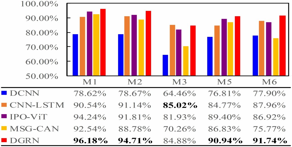
Fig. 6.: ACC of the trained models for each mode (M2, M3, M4, M5 and M6) in task T4.

T-SNE is used to visualize the feature maps. Taking task T1 as an example, M2 from test set 2 is selected for visualization.

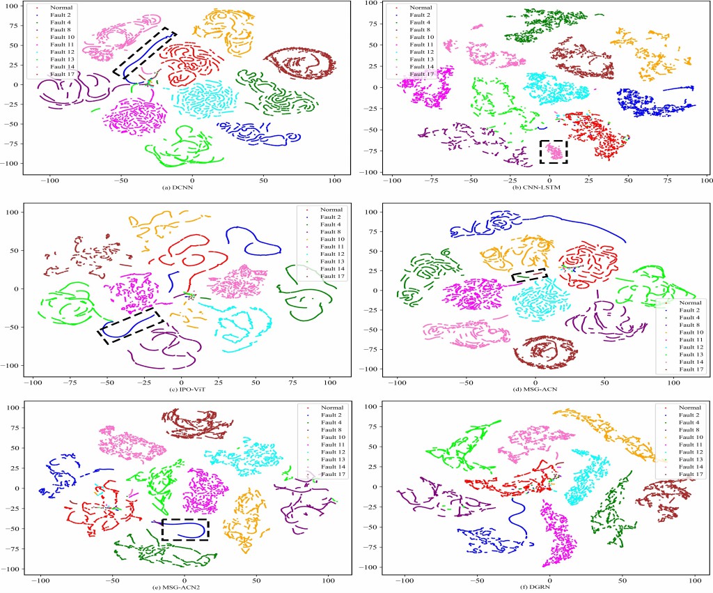
Fig. 7.: Feature visualization using T-SNE in task T1.

The results for each model are shown in Fig. 8. Colors represent fault classes, with a total of ten. The black dashed box highlights a set of samples that are clearly misclassified into other clusters. Such as Fault 2 samples in Fig. 8 (a), (c) and (e), Fault 4 and Fault 17 samples in Fig. 8 (d), and Fault 14 samples in Fig. 8 (b). Compared to other methods, the features extracted by DGRN effectively separate the boundaries between classes, with no significant overlap between different clusters. This facilitates the differentiation of fault classes, thereby validating the high generalization performance of DGRN.

The parameters of DCNN, CNN-LSTM, IPO-ViT, MSG-ACN, MSG-ACN2 and DGRN are counted as shown in Table 11, including the training and inference time spent. The proposed model DGRN requires fewer parameters, enabling faster training and inference.

Table 11: Parameter number, training and inference time spent of each model.

Evaluation metrics	DCNN	CNN- LSTM	IPO- ViT	MSG- ACN	MSG- ACN2	DGRN
No. of parameters in training process	11,404,334	895,330	26,378,350	680,034	2,316,426	1,944,039
Time spent on model training (s/epoch)	3.76	3.07	19.20	3.06	3.08	2.63
No. of parameters in inference process	11,404,334	895,330	26,378,350	645,002	645,002	645,002
Time spent on inference (s/epoch)	1.09	0.06	8.35	0.01	0.01	0.01

5.1.2 Ablation study

Ablation experiments were conducted to verify the effectiveness of pre-training, supervised contrastive learning, and adversarial learning. The pre-trained model is denoted as A1. A2 and A3 represent models where the supervised contrastive loss and discriminative loss are removed from DGRN, respectively. A4 represents DGRN without the pre-training process, optimized directly through training process. The hyperparameters for these models were obtained using Bayesian optimization, targeting the highest classification accuracy for pseudo-fault features. The classification accuracies of these different models on test set 2 are shown in Table 12.

Table 12: Results of ablation experiments.

Task No.	A1	A2	A3	A4	DGRN
T1	85.75%	91.76%	92.17%	91.95%	92.86%
T2	86.52%	92.44%	91.84%	92.61%	93.01%
T3	79.46%	84.19%	82.19%	86.72%	85.57%
T4	80.30%	90.53%	91.66%	91.53%	91.66%
T5	86.87%	91.23%	89.88%	91.56%	93.14%
T6	83.22%	86.12%	86.38%	85.99%	86.38%
Avg	83.69%	89.38%	89.02%	90.06%	90.44%

A2, A3 and DGRN are all improvements based on A1. They all show increased average classification accuracy compared to A1. This indicates that both discriminator and supervised contrastive learning contribute to the model’s generalization ability, and their combination achieved the optimal diagnostic results. DGRN has an average classification accuracy 0.38% higher than A4. This indicates that the pre-trained model can effectively guide to generate valid pseudo-fault features. In TE process scenario, pre-training, supervised contrastive learning, and adversarial learning strategies all contribute to enhancing the model’s ability to extract domain-invariant features. This confirms the high applicability of DGRN for fault diagnosis on unseen modes.

5.2 CSTR

5.2.1 Model comparison

Similar to TE experiment, six models were tested in the tasks shown in Table 5 respectively. Taking T3 as an example, the classification accuracy of DGRN on pseudo-fault features, test set 1 and test set 2 during the Bayesian optimization process are shown in Fig. 9. It can be observed that the maximum classification accuracy of pseudo-fault features is 99.65%. At this point, the classification accuracy on the test set 1 is 99.73%, and on test set 2 it is 96.92%. However, during the optimization process, the maximum classification accuracy on test set 2 is 97.87%. The results indicate that the optimized model still exhibits single-domain overfitting, and its generalization ability to unseen modes can be further improved.

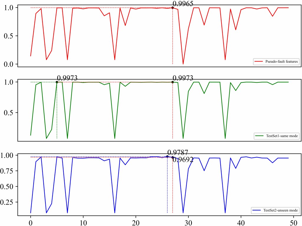
Fig. 8.: Classification accuracy on test set 1, test set 2, and pseudo-fault features during the Bayesian optimization process. ( Note that during the iteration process, some classification accuracies are less than 50%. This is due to the loss value becoming NaN, causing the optimization process to be interrupted.)

For the test set 1 of CSTR, the accuracies achieved by each model under different tasks are shown in Table 13. DGRN obtained the highest average classification accuracy. CNN-LSTM, MSG-ACN, MSG-ACN2 and DGRN all attained average classification accuracies higher than 99%, indicating that they have successfully acquired knowledge of single-mode faults in CSTR. Table 14 shows the experimental results on the test set 2. The average classification accuracy of MSG-ACN2 is higher than that of MSG-ACN, indicating that generating pseudo-fault features is more effective than generating unseen mode samples in CSTR scenario. MSG-ACN did not achieve good diagnostic performance in the CSTR scenario. This is hypothesized to be due to the small differences between some faulty and normal samples, making it difficult for the model to capture deep domain-invariant fault features. MSG-ACN2 achieved the highest classification accuracy in task T1. However, its average classification accuracy was 0.91% lower than that of DGRN. This indicates that MSG-ACN can only enhance the model’s generalization ability under specific unseen modes. DGRN achieved the highest classification accuracy in tasks T2 and T3, as well as the highest average classification accuracy. The comprehensive view shows that DGRN has superior diagnostic performance on unseen modes, confirming its outstanding ability to extract domain-invariant features.

Table 13: Experimental results on the test set 1 of CSTR (Accuracy).

Task No.	DCNN	CNN-LSTM	IPO-ViT	MSG-ACN	MSG-ACN2	DGRN
T1	89.82%	99.39%	98.32%	99.31%	99.39%	99.69%
T2	88.27%	99.35%	98.97%	99.31%	99.46%	99.77%
T3	91.20%	99.31%	98.09%	99.69%	99.50%	99.69%
Avg	89.76%	99.35%	98.46%	99.44%	99.45%	99.72%

Table 14: Experimental results on the test set 2 of CSTR (Accuracy).

Task No.	DCNN	CNN-LSTM	IPO-ViT	MSG-ACN	MSG-ACN2	DGRN
T1	87.18%	92.23%	95.49%	95.07%	97.66%	97.64%
T2	87.58%	95.19%	95.91%	96.86%	97.46%	98.20%
T3	85.55%	93.75%	93.16%	90.02%	94.91%	96.92%
Avg	86.77%	93.72%	94.85%	93.98%	96.68%	97.59%

Taking task T2 as an example, the confusion matrix for each model is shown in Fig. 10. The number of samples correctly classified by the DGRN is large, demonstrating the excellent performance of DGRN. M1 from test set 2 is selected for feature map visualization, as shown in Fig. 11. Thirteen colors represent thirteen different fault classes. In Fig. 11 (a), (b), (c), and (d), the dashed lines encircle a large number of overlapping samples from different classes. Such as F4 and F12 in Fig. 11 (a), F8 and F0 in Fig. 11 (b), (c) and (d). In Fig. 11(e), the dashed lines encircle the samples with low aggregation, which can be separated by the internal dashed line. As shown in Fig. 11(f), DGRN effectively distinguishes fault classes, with each class being more concentrated. Therefore, the proposed DGRN demonstrates good performance. The parameter number, training and inference time spent of each model are counted, as shown in Table 15. The proposed DGRN has fewer parameters, consumes less training time, and has faster inference.

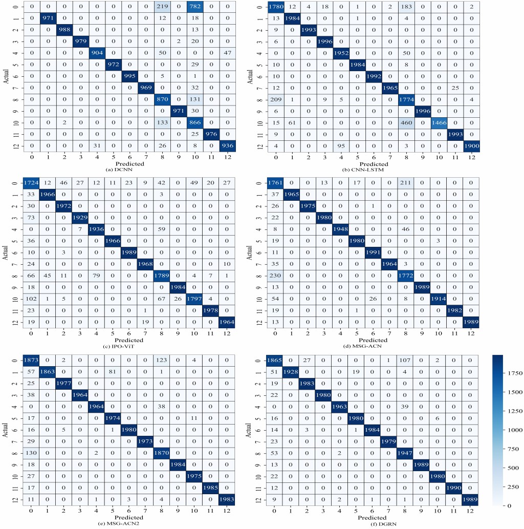
Fig. 9.: Confusion matrix for each model in the T2 task.

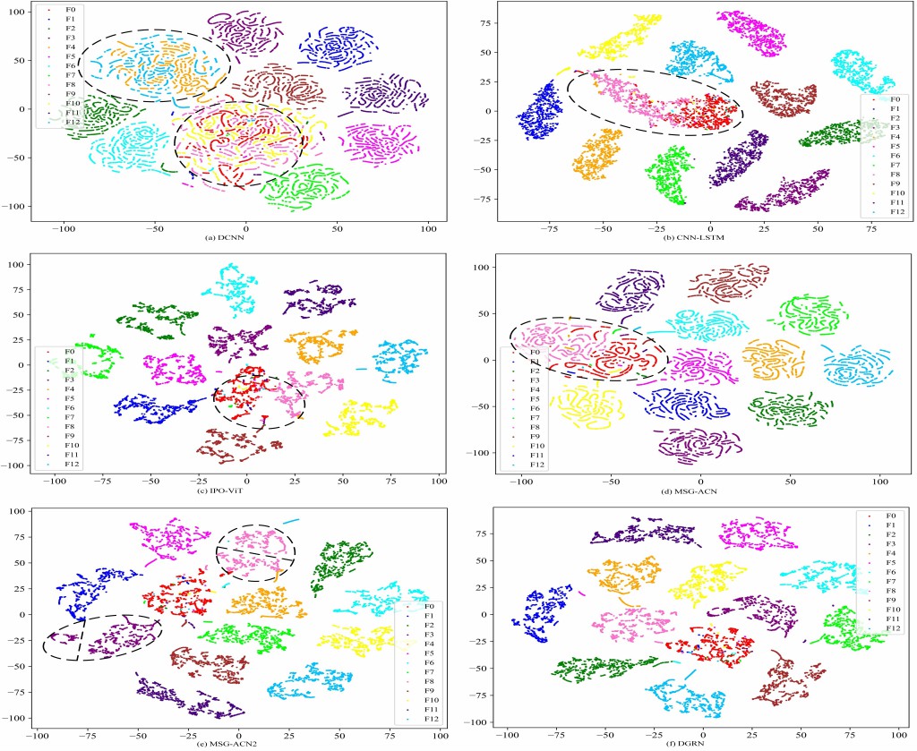
Fig. 10.: Feature visualization using T-SNE in task T2.

Table 15: Parameter number, training and inference time spent of each model.

Evaluation metrics	DCNN	CNN- LSTM	IPO- ViT	MSG- ACN	MSG- ACN2	DGRN
No. of parameters in training process	2,266,037	578,333	25,290,785	649,221	692,109	2,161,386
Time spent on model training (s/epoch)	2.49	3.04	9.89	2.86	2.83	2.53
No. of parameters in inference process	2,266,037	578,333	25,290,785	630,413	630,413	630,413
Time spent on inference (s/epoch)	0.019	0.027	8.67	0.005	0.006	0.006

5.2.2 Ablation study

The models used for the ablation study in the CSTR are consistent with those used in the TE process. The experimental results of each model on the test set 2 are shown in Table 16.

Comparing the classification accuracies of A1, A2, A3, and DGRN, it is evident that in the CSTR scenario, supervised contrastive learning consistently enhances diagnostic performance for unseen modes. Adversarial learning only improves the model’s generaliztion performance under certain specific mode. Combining both approaches yields the best diagnostic results. This indicates that supervised contrastive learning and adversarial learning have a mutually reinforcing effect, enhancing the model’s ability to learn domain-invariant features. The average classification accuracy of DGRN is 1.55% higher relative to A4, which confirms the function of pre-training. It helps to generate valid pseudo-fault features. Overall, combining pre-training strategies, supervised contrastive learning strategies, and adversarial learning strategies achieved the best average classification accuracy, verifying the model’s excellent generalization ability on unseen modes.

Table 16: Results of ablation experiments.

Task No.	A1	A2	A3	A4	DGRN
T1	97.19%	97.60%	96.68%	97.40%	97.64%
T2	97.61%	98.03%	97.67%	98.21%	98.20%
T3	96.07%	96.67%	95.30%	92.52%	96.92%
Avg	96.96%	97.43%	96.55%	96.04%	97.59%

6 Conclusion

In this paper, a single-domain generalization model in multi-mode fault diagnosis for process industrial systems is proposed. The novel method DGRN can generate pseudo-fault features with sufficient semantic consistency and domain diversity, which represent fault features from unseen modes. Meanwhile, domain-invariant fault knowledge is learned from single seen mode data fault features and pseudo-fault features, which can be applied to diagnose unseen mode samples. The experimental results on TE process and CSTR demonstrate the effectiveness of DGRN. Some conclusions are drawn below.

• The pseudo-fault features generation strategy avoids complex samples generation process, enhancing the model’s generalization ability to unseen mode data.

• Pre-training strategy can pre-extract fault features from a single condition. Then pseudo-fault features are generated by tranforming the pre-extract fault features. This prevents the generation of useless pseudo-fault features.

• The combination of adversarial learning with two gradient reversal layers and supervised contrastive learning achieves the generation of pseudo-fault features with sufficient diversity and semantic information, while also enabling the extraction of domain-invariant fault features.

• DGRN achieves robust generalization performance with fewer model parameters overall.

However, this paper considers the scenario where fault features are the same across multiple modes. Future work can address the issue of partial differences in fault features between single seen mode and multiple unseen modes. Furthermore, the presence of unknown faults and class imbalance in unseen modes are issues that require further research.

Appendix A Code Availability

https://github.com/GuangqiangLi/DGRN (it will be available after being published.)

References

- [1] W. J. Li, H. Li, S. Gu, T. Chen, Process fault diagnosis with model- and knowledge-based approaches: Advances and opportunities, Control Engineering Practice 105 (2020) 17. doi:10.1016/j.conengprac.2020.104637.
- [2] V. Venkatsubramanian, R. Rengaswamy, K. Yin, S. N. Kavuri, A review of process fault detection and diagnosis part i: Quantitative model-based methods, Computers & Chemical Engineering 27 (3) (2003) 293–311. doi:10.1016/s0098-1354(02)00160-6.
- [3] L. Chiang, E. Russell, R. Braatz, Fault detection and diagnosis in industrial systems, Springer London, 2000.
- [4] M. T. Amin, F. Khan, S. Ahmed, S. Imtiaz, Risk-based fault detection and diagnosis for nonlinear and non-gaussian process systems using r-vine copula, Process Safety and Environmental Protection 150 (2021) 123–136. doi:10.1016/j.psep.2021.04.010.
- [5] H. Ali, Z. Zhang, F. R. Gao, Multiscale monitoring of industrial chemical process using wavelet-entropy aided machine learning approach, Process Safety and Environmental Protection 180 (2023) 1053–1075. doi:10.1016/j.psep.2023.10.066.
- [6] X. T. Bi, R. S. Qin, D. Y. Wu, S. D. Zheng, J. S. Zhao, One step forward for smart chemical process fault detection and diagnosis, Computers & Chemical Engineering 164 (2022) 19. doi:10.1016/j.compchemeng.2022.107884.
- [7] L. H. Chiang, E. L. Russell, R. D. Braatz, Fault diagnosis in chemical processes using fisher discriminant analysis, discriminant partial least squares, and principal component analysis, Chemometrics and Intelligent Laboratory Systems 50 (2) (2000) 243–252. doi:10.1016/s0169-7439(99)00061-1.
- [8] J. M. Lee, C. K. Yoo, I. B. Lee, Statistical process monitoring with independent component analysis, Journal of Process Control 14 (5) (2004) 467–485. doi:10.1016/j.jprocont.2003.09.004.
- [9] Z. Q. Ge, Z. H. Song, Process monitoring based on independent component analysis-principal component analysis (ica-pca) and similarity factors, Industrial & Engineering Chemistry Research 46 (7) (2007) 2054–2063. doi:10.1021/ie061083g.
- [10] S. J. Qin, Statistical process monitoring: basics and beyond, Journal of Chemometrics 17 (8-9) (2003) 480–502. doi:10.1002/cem.800.
- [11] B. Song, S. Tan, H. B. Shi, B. Zhao, Fault detection and diagnosis via standardized k nearest neighbor for multimode process, Journal of the Taiwan Institute of Chemical Engineers 106 (2020) 1–8. doi:10.1016/j.jtice.2019.09.017.
- [12] Z. Yin, J. Hou, Recent advances on svm based fault diagnosis and process monitoring in complicated industrial processes, Neurocomputing 174 (2016) 643–650. doi:10.1016/j.neucom.2015.09.081.
- [13] Y. Q. Zhang, L. Luo, X. Ji, Y. Y. Dai, Improved random forest algorithm based on decision paths for fault diagnosis of chemical process with incomplete data, Sensors 21 (20) (2021) 20. doi:10.3390/s21206715.
- [14] N. Liu, M. G. Hu, J. Wang, Y. J. Ren, W. D. Tian, Fault detection and diagnosis using bayesian network model combining mechanism correlation analysis and process data: Application to unmonitored root cause variables type faults, Process Safety and Environmental Protection 164 (2022) 15–29. doi:10.1016/j.psep.2022.05.073.
- [15] M. T. Amin, F. Khan, S. Ahmed, S. Imtiaz, A data-driven bayesian network learning method for process fault diagnosis, Process Safety and Environmental Protection 150 (2021) 110–122. doi:10.1016/j.psep.2021.04.004.
- [16] C. Y. Lou, M. A. Atoui, X. S. Li, Novel online discriminant analysis based schemes to deal with observations from known and new classes: Application to industrial systems, Engineering Applications of Artificial Intelligence 111 (2022) 10. doi:10.1016/j.engappai.2022.104811.
- [17] Z. Y. Deng, T. Han, Z. H. Cheng, J. J. Jiang, F. J. Duan, Fault detection of petrochemical process based on space-time compressed matrix and naive bayes, Process Safety and Environmental Protection 160 (2022) 327–340. doi:10.1016/j.psep.2022.01.048.
- [18] Q. C. Tao, B. R. Xin, Y. F. Zhang, H. P. Jin, Q. Li, Z. D. Dai, Y. Y. Dai, A novel triage-based fault diagnosis method for chemical process, Process Safety and Environmental Protection 183 (2024) 1102–1116. doi:10.1016/j.psep.2024.01.072.
- [19] H. Wu, J. S. Zhao, Deep convolutional neural network model based chemical process fault diagnosis, Computers & Chemical Engineering 115 (2018) 185–197. doi:10.1016/j.compchemeng.2018.04.009.
- [20] Z. P. Zhang, J. S. Zhao, A deep belief network based fault diagnosis model for complex chemical processes, Computers & Chemical Engineering 107 (2017) 395–407. doi:10.1016/j.compchemeng.2017.02.041.
- [21] S. D. Zheng, J. S. Zhao, A new unsupervised data mining method based on the stacked autoencoder for chemical process fault diagnosis, Computers & Chemical Engineering 135 (2020) 17. doi:10.1016/j.compchemeng.2020.106755.
- [22] H. T. Zhao, S. Y. Sun, B. Jin, Sequential fault diagnosis based on lstm neural network, IEEE Access 6 (2018) 12929–12939. doi:10.1109/access.2018.2794765.
- [23] K. Zhou, Y. F. Tong, X. T. Li, X. R. Wei, H. Huang, K. Song, X. Chen, Exploring global attention mechanism on fault detection and diagnosis for complex engineering processes, Process Safety and Environmental Protection 170 (2023) 660–669. doi:10.1016/j.psep.2022.12.055.
- [24] C. Lou, M. A. Atoui, Unknown health states recognition with collective-decision-based deep learning networks in predictive maintenance applications, Mathematics 12 (1) (2024) 16. doi:10.3390/math12010089.
- [25] H. Hashim, P. Ryan, E. Clifford, A statistically based fault detection and diagnosis approach for non-residential building water distribution systems, Advanced Engineering Informatics 46 (2020) 15. doi:10.1016/j.aei.2020.101187.
- [26] T. Huang, Q. Zhang, X. A. Tang, S. Y. Zhao, X. N. Lu, A novel fault diagnosis method based on cnn and lstm and its application in fault diagnosis for complex systems, Artificial Intelligence Review 55 (2) (2022) 1289–1315. doi:10.1007/s10462-021-09993-z.
- [27] J. X. Zhang, Z. Miao, Z. M. Feng, R. F. Lv, C. Y. Lu, Y. Y. Dai, L. C. Dong, Gated recurrent unit-enhanced deep convolutional neural network for real-time industrial process fault diagnosis, Process Safety and Environmental Protection 175 (2023) 129–149. doi:10.1016/j.psep.2023.05.025.
- [28] Z. C. Wei, X. Ji, L. Zhou, Y. G. Dang, Y. Y. Dai, A novel deep learning model based on target transformer for fault diagnosis of chemical process, Process Safety and Environmental Protection 167 (2022) 480–492. doi:10.1016/j.psep.2022.09.039.
- [29] C. Lou, M. A. Atoui, X. Li, Recent deep learning models for diagnosis and health monitoring: A review of research works and future challenges, Transactions of the Institute of Measurement and Control (2023) 38doi:10.1177/01423312231157118.
- [30] M. Quinones-Grueiro, A. Prieto-Moreno, C. Verde, O. Llanes-Santiago, Data-driven monitoring of multimode continuous processes: A review, Chemometrics and Intelligent Laboratory Systems 189 (2019) 56–71. doi:10.1016/j.chemolab.2019.03.012.
- [31] S. J. Pan, Q. A. Yang, A survey on transfer learning, IEEE Transactions on Knowledge and Data Engineering 22 (10) (2010) 1345–1359. doi:10.1109/tkde.2009.191.
- [32] H. Wu, J. S. Zhao, Fault detection and diagnosis based on transfer learning for multimode chemical processes, Computers & Chemical Engineering 135 (2020) 13. doi:10.1016/j.compchemeng.2020.106731.
- [33] Y. L. Wang, D. Z. Wu, X. F. Yuan, Lda-based deep transfer learning for fault diagnosis in industrial chemical processes, Computers & Chemical Engineering 140 (2020) 13. doi:10.1016/j.compchemeng.2020.106964.
- [34] D. L. Gao, X. Z. Zhu, C. J. Yang, X. K. Huang, W. H. Wang, Deep weighted joint distribution adaption network for fault diagnosis of blast furnace ironmaking process, Computers & Chemical Engineering 162 (2022) 9. doi:10.1016/j.compchemeng.2022.107797.
- [35] Z. Chai, C. H. Zhao, A fine-grained adversarial network method for cross-domain industrial fault diagnosis, IEEE Transactions on Automation Science and Engineering 17 (3) (2020) 1432–1442. doi:10.1109/tase.2019.2957232.
- [36] J. D. Wang, C. L. Lan, C. Liu, Y. D. Ouyang, T. Qin, W. Lu, Y. Q. Chen, W. J. Zeng, P. S. Yu, Generalizing to unseen domains: a survey on domain generalization, IEEE Transactions on Knowledge and Data Engineering 35 (8) (2023) 8052–8072. doi:10.1109/tkde.2022.3178128.
- [37] Y. T. Xiao, H. B. Shi, B. Y. Wang, Y. Tao, S. Tan, B. Song, Fault diagnosis of unseen modes in chemical processes based on labeling and class progressive adversarial learning, IEEE Transactions on Instrumentation and Measurement 72 (2023) 12. doi:10.1109/tim.2022.3228271.
- [38] H. Huang, R. Wang, K. Zhou, L. Ning, K. Song, Causalvit: Domain generalization for chemical engineering process fault detection and diagnosis, Process Safety and Environmental Protection 176 (2023) 155–165. doi:10.1016/j.psep.2023.06.018.
- [39] Y. T. Xiao, H. B. Shi, B. Y. Wang, Y. Tao, S. Tan, B. Song, Weighted conditional discriminant analysis for unseen operating modes fault diagnosis in chemical processes, Ieee Transactions on Instrumentation and Measurement 71 (2022) 14. doi:10.1109/tim.2022.3152235.
- [40] C. Zhao, W. M. Shen, Adversarial mutual information-guided single domain generalization network for intelligent fault diagnosis, IEEE Transactions on Industrial Informatics 19 (3) (2023) 2909–2918. doi:10.1109/tii.2022.3175018.
- [41] J. Wang, H. Ren, C. Q. Shen, W. G. Huang, Z. K. Zhu, Multi-scale style generative and adversarial contrastive networks for single domain generalization fault diagnosis, Reliability Engineering & System Safety 243 (2024) 13. doi:10.1016/j.ress.2023.109879.
- [42] Y. Y. Pu, J. Tang, X. G. Li, C. Wei, W. B. Huang, X. X. Ding, Single-domain incremental generation network for machinery intelligent fault diagnosis under unknown working speeds, Advanced Engineering Informatics 60 (2024) 14. doi:10.1016/j.aei.2024.102400.
- [43] Y. Guo, J. Zhang, Chemical fault diagnosis network based on single domain generalization, Process Safety and Environmental Protection 188 (2024) 1133–1144. doi:https://doi.org/10.1016/j.psep.2024.05.106.
- [44] L. A. Gatys, A. S. Ecker, M. Bethge, Ieee, Image style transfer using convolutional neural networks, in: 2016 IEEE Conference on Computer Vision and Pattern Recognition (CVPR), IEEE Conference on Computer Vision and Pattern Recognition, Ieee, NEW YORK, 2016, pp. 2414–2423. doi:10.1109/cvpr.2016.265.
- [45] X. Glorot, A. Bordes, Y. Bengio, Deep sparse rectifier neural networks, in: Proceedings of the Fourteenth International Conference on Artificial Intelligence and Statistics, JMLR Workshop and Conference Proceedings, 2011, pp. 315–323.
- [46] M. Long, Z. Cao, J. Wang, M. I. Jordan, Conditional adversarial domain adaptation, Advances in Neural Information Processing Systems 31 (2018).
- [47] P. Khosla, P. Teterwak, C. Wang, A. Sarna, Y. Tian, P. Isola, A. Maschinot, C. Liu, D. Krishnan, Supervised contrastive learning, Advances in Neural Information Processing Systems 33 (2020) 18661–18673.
- [48] J. J. Downs, E. F. Vogel, A plant-wide industrical-process control problem, Computers & Chemical Engineering 17 (3) (1993) 245–255. doi:10.1016/0098-1354(93)80018-i.
- [49] K. E. S. Pilario, Y. Cao, Canonical variate dissimilarity analysis for process incipient fault detection, IEEE Transactions on Industrial Informatics 14 (12) (2018) 5308–5315. doi:10.1109/tii.2018.2810822.
- [50] A. Bathelt, N. L. Ricker, M. Jelali, Revision of the tennessee eastman process model, IFAC-PapersOnLine 48 (8) (2015) 309–314. doi:10.1016/j.ifacol.2015.08.199.
- [51] Z. Y. Liu, C. Li, X. He, Evidential ensemble preference-guided learning approach for real-time multimode fault diagnosis, IEEE Transactions on Industrial Informatics 20 (4) (2024) 5495–5504. doi:10.1109/tii.2023.3332112.