A Unified Confidence Sequence for Generalized Linear Models, with Applications to Bandits

Abstract

We present a unified likelihood ratio-based confidence sequence (CS) for any (self-concordant) generalized linear models (GLMs) that is guaranteed to be convex and numerically tight. We show that this is on par or improves upon known CSs for various GLMs, including Gaussian, Bernoulli, and Poisson. In particular, for the first time, our CS for Bernoulli has a $\operatorname{poly}(S)$-free radius where $S$ is the norm of the unknown parameter. Our first technical novelty is its derivation, which utilizes a time-uniform PAC-Bayesian bound with a uniform prior/posterior, despite the latter being a rather unpopular choice for deriving CSs. As a direct application of our new CS, we propose a simple and natural optimistic algorithm called OFUGLB applicable to any generalized linear bandits (GLB; Filippi et al. (2010)). Our analysis shows that the celebrated optimistic approach simultaneously attains state-of-the-art regrets for various self-concordant (not necessarily bounded) GLBs, and even $\operatorname{poly}(S)$-free for bounded GLBs, including logistic bandits. The regret analysis, our second technical novelty, follows from combining our new CS with a new proof technique that completely avoids the previously widely used self-concordant control lemma (Faury et al., 2020, Lemma 9). Finally, we verify numerically that OFUGLB significantly outperforms the prior state-of-the-art (Lee et al., 2024) for logistic bandits.

1 Introduction

One paramount task in statistics and machine learning is to estimate the uncertainty of the underlying model from (possibly noisy) observations. For example, in interactive machine learning scenarios such as bandits (Thompson, 1933; Robbins, 1952; Lattimore and Szepesvári, 2020) and recently reinforcement learning with human feedback (RLHF; Ouyang et al. (2022); Christiano et al. (2017)), at each time step $t$, the learner chooses an action ${\bm{x}}_{t}$ from an available set of actions $\mathcal{X}_{t}$ and observes reward or outcome $r_{t}$ that is modeled as a distribution whose mean is an unknown function $f^{*}$ of ${\bm{x}}_{t}$; i.e., $r_{t}\sim p(\cdot|{\bm{x}}_{t};f^{*})$. One popular choice of such a model is generalized linear model (GLM; McCullagh and Nelder (1989)) that extends exponential family distributions to have linear structure in its natural parameter, i.e., $\langle{\bm{x}},\bm{\theta}_{\star}\rangle$ where $\bm{\theta}_{\star}$ is an unknown parameter, which means that the mean function is $f^{*}({\bm{x}})=\mu(\langle{\bm{x}},\bm{\theta}_{\star}\rangle)$ for some inverse link function $\mu$. This encompasses a wide range of distributions, which in turn makes it ubiquitous in various real-world applications, such as news recommendations (Bernoulli; Li et al. (2010, 2012)), social network influence maximization (Poisson; Lage et al. (2013); Gisselbrecht et al. (2015)), and more. In such tasks, the learner must estimate the uncertainty about $\bm{\theta}_{\star}$ at each time step $t\geq 1$, given observations $\{({\bm{x}}_{s},r_{s})\}_{s=1}^{t-1}$, to make wise decisions. One popular and useful way to capture the uncertainty is via a time-uniform confidence sequence (CS) $\{\mathcal{C}_{t}(\delta)\}_{t=1}^{\infty}$, which takes the form of ${\mathbb{P}}[\exists t\geq 1\mathrel{\mathop{\mathchar 58\relax}}\bm{\theta}_{\star}\not\in{\mathcal{C}}_{t}(\delta)]\leq\delta$. Recently, CS has been described as one of the key components for safe anytime-valid inference (SAVI) that can ensure the validity/safeness of sequentially adaptive statistical inference (Ramdas et al., 2023).

There has been much work on deriving CS for specific families of distributions. Many common distributions are in a smaller family, called generalized linear models (GLMs). Existing CSs for GLM, however, are far from ideal. Much of the prior works focus on obtaining CS for specific instantiations of GLMs, such as Gaussian (Abbasi-Yadkori et al., 2011; Flynn et al., 2023) and Bernoulli (Faury et al., 2020; Abeille et al., 2021; Faury et al., 2022; Lee et al., 2024). Especially for Bernoulli, all the existing CSs suffer from $\operatorname{poly}(S)$ factor in the radius, where $S$ is the norm of the unknown parameter $\bm{\theta}_{\star}$. Jun et al. (2017); Li et al. (2017); Emmenegger et al. (2023) proposed generic CSs that work for any convex GLMs, but their radii all suffer from a globally worst-case curvature of $\mu$, which is detrimental in many cases (e.g., for Bernoulli, it scales as $e^{S}$).

Contributions.

First, we propose a unified construction of likelihood ratio-based CS for any convex GLMs (Theorem 3.1) and then instantiate it as an ellipsoidal CS for self-concordant GLMs, including Bernoulli, Gaussian, and Poisson distributions (Theorem 3.2). Notably, we keep track of all the constants so that any practitioner can directly implement it without trouble. The proof uses ingredients from time-uniform PAC-Bayesian bounds (Chugg et al., 2023) – martingale + Donsker-Varadhan representation of KL + Ville’s inequality. The main technical novelty lies in using uniform prior/posterior for the analysis, inspired by various literature on portfolios (Blum and Kalai, 1999) and fast rates in statistical/online learning (Foster et al., 2018; van Erven et al., 2015; Grünwald and Mehta, 2020; Hazan et al., 2007).

Secondly, we apply our novel CSs to contextual generalized linear bandits (GLB; Filippi et al. (2010)) with changing (and adversarial) arm sets, and propose a new algorithm called Optimism in the Face of Uncertainty for Generalized Linear Bandits (OFUGLB). OFUGLB employs the simple and standard optimistic approach, choosing an arm that maximizes the upper confidence bound (UCB) computed by our CS (Auer, 2002; Abbasi-Yadkori et al., 2011). We show that OFUGLB achieves the state-of-the-art regret bounds for self-concordant (possibly unbounded) GLB (Theorem 4.1). This is the first time a computationally tractable, purely optimistic strategy attains such $\operatorname{poly}(S)$-free regret for logistic bandits in that OFUGLB does not involve an explicit warmup phase and only involves convex optimization subroutines. Our other significant main technical contribution is the analysis of OFUGLB since naïvely applying existing analysis techniques for optimistic algorithms (Lee et al., 2024; Abeille et al., 2021) yields a regret bound whose leading term scales with $\operatorname{poly}(S)$. We identify the key reason for such additional dependency as the use of self-concordance control lemma (Faury et al., 2020, Lemma 9), and provide an alternate analysis that completely bypasses it, which may be of independent interest in the bandits community and beyond.

2 Problem Setting

We consider the realizable (online) regression with the generalized linear model (GLM; McCullagh and Nelder (1989)) whose conditional density of $r$ is given as

$$dp(r|{\bm{x}};\bm{\theta}_{\star})=\exp\left(\frac{r\langle{\bm{x}},\bm{\theta}_{\star}\rangle-m(\langle{\bm{x}},\bm{\theta}_{\star}\rangle)}{g(\tau)}+h(r,\tau)\right)d\nu,$$ (1)

where $\tau$ is some known scaling (temperature) parameter and $\nu$ is some known base measure (e.g., Lebesgue, counting). We assume the following:

Assumption 1.

The domain $X$ for arm (context) ${\bm{x}}$ satisfies $X\subseteq{\mathcal{B}}^{d}(1)$.

Assumption 2.

$\bm{\theta}_{\star}\in\Theta\subseteq{\mathcal{B}}^{d}(S)\mathrel{\mathop{\mathchar 58\relax}}=\{\bm{\theta}\in{\mathbb{R}}^{d}\mathrel{\mathop{\mathchar 58\relax}}\left\lVert\bm{\theta}\right\rVert_{2}\leq S\}$ for some known $S>0$. Also, $\Theta$ is nonempty, compact, and convex with intrinsic dimension $d$.

Assumption 3.

$m$ is three times differentiable and convex, i.e., $m^{\prime\prime\prime}$ exists and $\dot{\mu}\mathrel{\mathop{\mathchar 58\relax}}=m^{\prime\prime}\geq 0$.

In the generalized linear bandit (GLB) problem, at each time $t\in[T]$, the learner observes a time-varying, arbitrary (often called adversarial) arm set ${\mathcal{X}}_{t}\subseteq X$, chooses a ${\bm{x}}_{t}\in{\mathcal{X}}_{t}$, and receives a reward $r_{t}\sim p(\cdot|{\bm{x}}_{t},\bm{\theta}_{\star})$. Let $\mathcal{X}_{[T]}\mathrel{\mathop{\mathchar 58\relax}}=\cup_{t=1}^{T}\mathcal{X}_{t}$ and $\Sigma_{t+1}\mathrel{\mathop{\mathchar 58\relax}}=\sigma(\Sigma_{t},r_{t},{\bm{x}}_{t+1})$ with $\Sigma_{0}=\sigma({\bm{x}}_{1})$ be the filtration in the canonical bandit model (Lattimore and Szepesvári, 2020, Chapter 4.6). From well-known properties of GLMs (McCullagh and Nelder, 1989), we have that $\mathbb{E}[r_{t}|\Sigma_{t}]=m^{\prime}(\langle{\bm{x}}_{t},\bm{\theta}_{\star}\rangle)\triangleq\mu(\langle{\bm{x}}_{t},\bm{\theta}_{\star}\rangle)$ and $\mathrm{Var}[r_{t}|\Sigma_{t}]=g(\tau)\dot{\mu}(\langle{\bm{x}}_{t},\bm{\theta}_{\star}\rangle)$, where $\mu$ is the inverse link function. We also define the following quantity describing the maximum slope of $\mu$:

$$R_{\dot{\mu}}\mathrel{\mathop{\mathchar 58\relax}}=\max_{{\bm{x}}\in\mathcal{X}_{[T]},\bm{\theta}\in\Theta}\dot{\mu}(\langle{\bm{x}},\bm{\theta}\rangle).$$ (2)

Note that many common distributions, such as Gaussian ($\mu(z)=z$), Poisson ($\mu(z)=e^{z}$), and Bernoulli ($\mu(z)=(1+e^{-z})^{-1}$), fall under the umbrella of GLM.

3 Unified Likelihood Ratio-based Confidence Sequence for GLMs

The learner’s goal is to output a time-uniform confidence sequence (CS) for $\bm{\theta}_{\star}$, ${\mathbb{P}}[\exists t\geq 1\mathrel{\mathop{\mathchar 58\relax}}\bm{\theta}_{\star}\not\in{\mathcal{C}}_{t}(\delta)]\leq\delta$, where ${\mathbb{P}}$ is w.r.t. the randomness of the confidence sets ${\mathcal{C}}_{t}(\delta)$. In this work, we are particularly interested in the log-likelihood-based confidence set “centered” at the norm-constrained, batch maximum likelihood estimator (MLE):

$${\mathcal{C}}_{t}(\delta)\mathrel{\mathop{\mathchar 58\relax}}=\left\{\bm{\theta}\in\Theta\mathrel{\mathop{\mathchar 58\relax}}{\mathcal{L}}_{t}(\bm{\theta})-{\mathcal{L}}_{t}(\widehat{\bm{\theta}}_{t})\leq{\color[rgb]{0,0,1}\beta_{t}(\delta)^{2}}\right\},$$ (3)

where $\beta_{t}(\delta)^{2}$ is the “radius” of the CS that we will define later, and ${\mathcal{L}}_{t}(\bm{\theta})$ is the negative log-likelihood of $\bm{\theta}$ w.r.t. data collected up to $t-1$, and

$${\mathcal{L}}_{t}(\bm{\theta})\mathrel{\mathop{\mathchar 58\relax}}=\sum_{s=1}^{t-1}\left\{\ell_{s}(\bm{\theta})\triangleq\frac{-r_{s}\langle{\bm{x}}_{s},\bm{\theta}\rangle+m(\langle{\bm{x}}_{s},\bm{\theta}\rangle)}{g(\tau)}\right\},\quad\widehat{\bm{\theta}}_{t}\mathrel{\mathop{\mathchar 58\relax}}=\operatorname*{arg\,min}_{\bm{\theta}\in\Theta}{\mathcal{L}}_{t}(\bm{\theta}).$$ (4)

Note that $h(r_{s},\tau)$ is omitted as it plays no role in the confidence set nor the MLE.

The form of the confidence set is the same as Lee et al. (2024) in that it leverages the batched constrained MLE as opposed to the batch regularized MLE (Abbasi-Yadkori et al., 2011), sequential (regularized) MLE (Abbasi-Yadkori et al., 2012; Jun et al., 2017; Emmenegger et al., 2023; Faury et al., 2022; Wasserman et al., 2020), or expected loss over some distribution (e.g., Gaussian) without committing to an estimator (Flynn et al., 2023). As one can see later, our derivation of the CS also starts from an expectation of loss over a prior distribution of ${\bm{\theta}}$ without committing to an estimator, yet we introduce the estimator to avoid the computational difficulty of evaluating the expectation.

Our first main contribution is the following unified confidence sequence for any GLMs, regardless of whether it is bounded or not, as long as the corresponding log-likelihood loss is Lipschitz:

Practically, the computation of $L_{t}$ involves a potentially non-concave maximization over a convex set, which is NP-hard in general (Murty and Kabadi, 1987). In Table 1, we provide closed-form (up to absolute constants), high-probability upper bounds for $L_{t}$’s for various GLMs:

Table 1: Instantiations of $L_{t}$’s for various GLMs. For Gaussian and Poisson, we omit the absolute constants for simplicity; these are made explicit in the proofs. “Bounded by $M$” means $\max_{{\bm{x}}\in\mathcal{X}_{[T]},\bm{\theta}\in\Theta}|r-\mu(\langle{\bm{x}},\bm{\theta}_{\star}\rangle)|\leq M<\infty$.

GLM	Upper bounds for $L_{t}$	Proof
Bounded by $M$	$(M+2SR_{\dot{\mu}})(t-1)/g(\tau)$	Trivial from triangle inequality
Bernoulli	$(1+S/2)(t-1)$	Trivial from above
Gaussian	$\sigma^{-2}\left(St+\sigma\sqrt{t\log\frac{d}{\delta}}\right)$	Appendix A.1
Poisson	$e^{S}t+\log\frac{d}{\delta}$	Appendix A.2

Comparisons to Prior Works.

There have been some works on providing CSs for either generic GLMs (Emmenegger et al., 2023; Jun et al., 2017; Li et al., 2017) or specific GLMs (linear: Flynn et al. (2023), logistic: Faury et al. (2020); Abeille et al. (2021); Lee et al. (2024)). The generic CSs are generally not tight as the “radius” often scales with $\kappa\mathrel{\mathop{\mathchar 58\relax}}=\left(\min_{{\bm{x}}\in X,\bm{\theta}\in\Theta}\dot{\mu}(\langle{\bm{x}},\bm{\theta}\rangle)\right)^{-1}$, which scales exponentially in $S$ for Bernoulli (Faury et al., 2020). For instance, Theorem 1 of Jun et al. (2017) and Theorem 1 of Li et al. (2017) proved CSs of the form $\left\lVert\bm{\theta}-\widehat{\bm{\theta}}_{t}\right\rVert_{{\bm{V}}_{t}}^{2}\leq\zeta_{1}(t,\delta)$, with $\zeta_{1}$ always scaling with $\kappa$. Emmenegger et al. (2023) proposed a CS using weighted, sequential likelihood testing that is empirically shown to be superior to other approaches. However, their Theorem 3, which rewrites the likelihood-based CS as the form $D(\bm{\theta},\bm{\theta}_{\star})\leq\zeta_{2}(t,\delta)$ for some well-defined Bregman divergence $D(\cdot,\cdot)$ and $\zeta_{2}$, always scales with $\kappa$ as well and thus a direct comparison with our CS is not possible. Interested readers are referred to Section 3.3 for further discussions on CSs for exponential family. On the other hand, the CSs for specific GLMs are inapplicable to GLM models beyond what they are designed for and may not be tight enough. For the Bernoulli distribution, the prior state-of-the-art (likelihood ratio-based) CS radius is ${\mathcal{O}}\left(S\log\frac{1}{\delta}+d\log\frac{St}{d}\right)$ of Lee et al. (2024), while our theorem gives us ${\mathcal{O}}\left(\log\frac{1}{\delta}+d\log\frac{St}{d}\right)$. We completely remove the $\operatorname{poly}(S)$-dependency from the radius, resolving one of the open problems posited by Lee et al. (2024). Later in Section 4, we show that this improvement is significant, both theoretically and numerically, for logistic bandits.

3.1 Ellipsoidal Confidence Sequence for Self-Concordant GLMs

Having an ellipsoidal version of CS is often beneficial, as this is easier to implement in practice. In particular, in the context of bandits, this allows one to equivalently rewrite the optimistic optimization in the UCB algorithm as a closed-form bonus-based UCB algorithm, even if the MLE requires an iterative algorithm. This section provides the ellipsoidal version of Theorem 3.1 for the following class of GLMs whose inverse link function $\mu$ satisfies the following:

Assumption 4 (Russac et al. (2021)).

$\mu$ is (generalized) self-concordant, i.e., the following quantity is well-defined (finite): $R_{s}\mathrel{\mathop{\mathchar 58\relax}}=\inf\left\{R\geq 0\mathrel{\mathop{\mathchar 58\relax}}|\ddot{\mu}(\langle{\bm{x}},\bm{\theta}\rangle)|\leq R\dot{\mu}(\langle{\bm{x}},\bm{\theta}\rangle),\ \forall{\bm{x}}\in X,\bm{\theta}\in\Theta\right\}$.

For instance, Bernoulli satisfies this with $R_{s}=1$, and more generally, GLM bounded by $R$ a.s. satisfy this assumption with $R_{s}=R$ (Sawarni et al., 2024, Lemma 2.1). Many unbounded GLMs also satisfy this assumption, such as Gaussian ($\mu(z)=z\Rightarrow R_{s}=0$), Poisson ($\mu(z)=e^{z}\Rightarrow R_{s}=1$), and Exponential ($\mu(z)=1\Rightarrow R_{s}=0$).

For this class of GLMs, we have the following slightly relaxed ellipsoidal CS, whose proof is deferred to Appendix A.3:

Let us denote $A\lesssim B$ if $A\leq cB$ for some absolute constant $c>0$. Note that the relaxation is “strict” (i.e., Theorem 3.2 is strictly looser than Theorem 3.1) when $R_{s}>0$. For Gaussian distribution, we have that $R_{s}=0$; thus, the ellipsoidal relaxation is exact! We then have that $\nabla^{2}{\mathcal{L}}_{t}(\widehat{\bm{\theta}}_{t})=\frac{1}{\sigma^{2}}\sum_{s=1}^{t-1}{\bm{x}}_{s}{\bm{x}}_{s}^{\top}=\mathrel{\mathop{\mathchar 58\relax}}\frac{1}{\sigma^{2}}{\bm{V}}_{t}$, and $L_{t}\lesssim St$ with high probability (Proposition A.1). Combining everything, we have $\left\lVert\bm{\theta}-\widehat{\bm{\theta}}_{t}\right\rVert_{{\bm{V}}_{t}}^{2}\lesssim\sigma^{2}\left(\log\frac{t}{\delta}+d\log\frac{St}{d}\right)$, which completely matches the prior state-of-the-art radius as in Lemma D.10 of Flynn et al. (2023) with $c=\sigma^{2}S^{2}$.

3.2 Proof of Theorem 3.1 – PAC-Bayes Approach with Uniform Prior

We consider $M_{t}(\bm{\theta})\mathrel{\mathop{\mathchar 58\relax}}=\exp\left({\mathcal{L}}_{t}(\bm{\theta}_{\star})-{\mathcal{L}}_{t}(\bm{\theta})\right),$ the log-likelihood ratio between the (estimated) distribution corresponding to $\bm{\theta}$ and the true distribution corresponding to $\bm{\theta}_{\star}$. This has been the subject of study for over 50 years  (Robbins and Siegmund, 1972; Lai, 1976; Darling and Robbins, 1967a, b) and recently revisited by statistics and machine learning communities (Ramdas et al., 2023; Emmenegger et al., 2023; Wasserman et al., 2020; Flynn et al., 2023).

We follow the usual recipes for deriving time-uniform PAC-Bayesian bound (Chugg et al., 2023; Alquier, 2024). We start with the following time-uniform property:

Lemma 3.1.

Let $\delta\in(0,1)$. For any data-independent probability measure ${\mathbb{Q}}$ on $\Theta$, we have:

$${\mathbb{P}}\left(\exists t\geq 1\mathrel{\mathop{\mathchar 58\relax}}\mathbb{E}_{\bm{\theta}\sim{\mathbb{Q}}}[M_{t}(\bm{\theta})]\geq\frac{1}{\delta}\right)\leq\delta,$$ (7)

where ${\mathbb{P}}$ is over the randomness of the data (and thus randomness of ${\mathcal{L}}_{t}$’s).

Proof.

First, it is easy to see that $M_{t}(\bm{\theta})=\prod_{s=1}^{t}\frac{dp(r_{s}|x_{s};\bm{\theta})}{dp(r_{s}|x_{s};\bm{\theta}_{\star})}$ is a nonnegative martingale w.r.t. $\Sigma_{t}$:

$$\mathbb{E}[M_{t}(\bm{\theta})|\Sigma_{t-1}]=M_{t-1}(\bm{\theta})\mathbb{E}\left[\frac{dp(r_{t}|x_{t};\bm{\theta})}{dp(r_{t}|x_{t};\bm{\theta}_{\star})}\bigg{|}\Sigma_{t-1}\right]=M_{t-1}(\bm{\theta})\underbrace{\int_{\mathcal{R}}\frac{dp(r|x_{t};\bm{\theta})}{dp(r|x_{t};\bm{\theta}_{\star})}dp(r|x_{t};\bm{\theta}_{\star})}_{=1},$$

where ${\mathcal{R}}$ is the support of the GLM. (Note that this holds for any distributions.)

Now consider the random variable $\mathbb{E}_{\bm{\theta}\sim{\mathbb{Q}}}[M_{t}(\bm{\theta})]$, which is adapted to $\Sigma_{t}$. This is a martingale, as

$$\mathbb{E}[\mathbb{E}_{\bm{\theta}\sim{\mathbb{Q}}}[M_{t}(\bm{\theta})]|\Sigma_{t-1}]\overset{(*)}{=}\mathbb{E}_{\bm{\theta}\sim{\mathbb{Q}}}[\mathbb{E}[M_{t}(\bm{\theta})|\Sigma_{t-1}]]=\mathbb{E}_{\bm{\theta}\sim{\mathbb{Q}}}[M_{t-1}(\bm{\theta})]$$

where $(*)$ follows from Tonelli’s theorem. We conclude by Ville’s inequality (Ville, 1939). ∎

We recall the variational representation of the KL divergence:

Lemma 3.2 (Theorem 2.1 of Donsker and Varadhan (1983)).

For two probability measures ${\mathbb{P}},{\mathbb{Q}}$ over $\Theta$, we have the following: $D_{\mathrm{KL}}({\mathbb{P}}||{\mathbb{Q}})=\sup_{g\mathrel{\mathop{\mathchar 58\relax}}\Theta\rightarrow{\mathbb{R}}}\mathbb{E}_{\bm{\theta}\sim{\mathbb{P}}}[g(\bm{\theta})]-\log\mathbb{E}_{\bm{\theta}\sim{\mathbb{Q}}}[e^{g(\bm{\theta})}]$.

We then have the following:

Lemma 3.3.

For any data-independent prior ${\mathbb{Q}}$ and any sequence of adapted posterior distributions (possibly learned from the data) $\{{\mathbb{P}}_{t}\}$, the following holds: for any $\delta\in(0,1)$,

$${\mathbb{P}}\left(\exists t\geq 1\mathrel{\mathop{\mathchar 58\relax}}{\mathcal{L}}_{t}(\bm{\theta}_{\star})-\mathbb{E}_{\bm{\theta}\sim{\mathbb{P}}_{t}}[{\mathcal{L}}_{t}(\bm{\theta})]\geq\log\frac{1}{\delta}+D_{\mathrm{KL}}({\mathbb{P}}_{t}||{\mathbb{Q}})\right)\leq\delta.$$ (8)

Proof.

Note that

$$\log\mathbb{E}_{\bm{\theta}\sim{\mathbb{Q}}}[M_{t}(\bm{\theta})]-{\mathcal{L}}_{t}(\bm{\theta}_{\star})=\log\mathbb{E}_{\bm{\theta}\sim{\mathbb{Q}}}[\exp\left(-{\mathcal{L}}_{t}(\bm{\theta})\right)]\overset{(*)}{\geq}\mathbb{E}_{\bm{\theta}\sim{\mathbb{P}}_{t}}[-{\mathcal{L}}_{t}(\bm{\theta})]-D_{\mathrm{KL}}({\mathbb{P}}_{t}||{\mathbb{Q}}),$$

where $(*)$ follows from Lemma 3.2 with $g(\cdot)=-{\mathcal{L}}_{t}(\cdot)$. By Lemma 3.1, we have that ${\mathbb{P}}\left(\exists t\geq 1\mathrel{\mathop{\mathchar 58\relax}}\log\frac{1}{\delta}\leq\log\mathbb{E}_{\bm{\theta}\sim{\mathbb{Q}}}[M_{t}(\bm{\theta})]\right)\leq\delta$. Rearranging gives the desired statement. ∎

Remark 1 (Choice of KL).

One can replace KL with other divergences with similar variational formulations (Ohnishi and Honorio, 2021). As we will show later, KL suffices for our purpose.

Up to now, it is well-known in the PAC-Bayes literature. Our main technical novelty lies in how to choose ${\mathbb{Q}}$ and ${\mathbb{P}}_{t}$, which is as follows: for $c\in(0,1]$ to be determined later, we set

$${\mathbb{Q}}=\mathrm{Unif}(\Theta),\quad{\mathbb{P}}_{t}=\mathrm{Unif}(\widetilde{\Theta}_{t}\triangleq(1-c)\widehat{\bm{\theta}}_{t}+c\Theta),$$ (9)

where $\mathrm{Unif}(\cdot)$ is the uniform distribution and ${\bm{a}}+\Theta=\{{\bm{a}}+\bm{\theta}\mathrel{\mathop{\mathchar 58\relax}}\bm{\theta}\in\Theta\}$ for a vector ${\bm{a}}\in{\mathbb{R}}^{d}$.

Then, denoting $\mathrm{vol}(\cdot)$ as the (Lebesgue) volume in ${\mathbb{R}}^{d}$, we have

$$D_{\mathrm{KL}}({\mathbb{P}}_{t}||{\mathbb{Q}})=\log\frac{\mathrm{vol}(\Theta)}{\mathrm{vol}(\widetilde{\Theta})}=\log\frac{\mathrm{vol}(\Theta)}{\mathrm{vol}\left((1-c)\widehat{\bm{\theta}}_{t}+c\Theta\right)}=\log\frac{\mathrm{vol}(\Theta)}{\mathrm{vol}(c\Theta)}=\log\frac{\mathrm{vol}(\Theta)}{c^{d}\mathrm{vol}(\Theta)}=d\log\frac{1}{c}.$$

We also have that

$$\mathbb{E}_{\bm{\theta}\sim{\mathbb{P}}_{t}}[{\mathcal{L}}_{t}(\bm{\theta})]={\mathcal{L}}_{t}(\widehat{\bm{\theta}}_{t})+\mathbb{E}_{\bm{\theta}\sim{\mathbb{P}}_{t}}[{\mathcal{L}}_{t}(\bm{\theta})-{\mathcal{L}}_{t}(\widehat{\bm{\theta}}_{t})]\leq{\mathcal{L}}_{t}(\widehat{\bm{\theta}}_{t})+2SL_{t}c,$$

where the last inequality follows from the Lipschitzness of ${\mathcal{L}}_{t}(\cdot)$ and the observation that for $\bm{\theta}=(1-c)\widehat{\bm{\theta}}_{t}+c\tilde{\bm{\theta}}\in\widetilde{\Theta}_{t}$, $\left\lVert\bm{\theta}-\widehat{\bm{\theta}_{t}}\right\rVert_{2}=c\left\lVert\tilde{\bm{\theta}}-\widehat{\bm{\theta}_{t}}\right\rVert_{2}\leq 2Sc$. We conclude by minimizing over $c\in(0,1]$. ∎

Remark 2 (Our choice of posterior).

The main intuition behind the translated/shrunken posterior is to show that a sufficiently large volume of $\Theta$ is sufficiently near $\widehat{\bm{\theta}}_{t}$. Indeed, in the literature, such choice has been considered for the first time in proof of Theorem 1 of Blum and Kalai (1999), and later in fast rates in online learning (Hazan et al., 2007; Foster et al., 2018). To our knowledge, this is the first time such a translated/shrunken posterior has been used in the PAC-Bayes context.

3.3 Relations to Prior Works

CSs for Exponential Family.

Lai (1976) derived the first generic CS for the exponential family based on a generalized likelihood ratio. Their CS, however, only applies to scalar-valued unknown parameters, and instantiating it often requires solving an equation with no closed-form solution (e.g., $f_{n}$ and $g_{n}$ in Lai (1976)). Recently, Chowdhury et al. (2023) proposed a generic CS for exponential family expressed in the local Bregman geometry induced by the log-partition function. The proof relies on the method of mixtures (Kaufmann and Koolen, 2021; de la Peña et al., 2004), which resembles our PAC-Bayesian approach that utilizes a mixture of log-likelihood functions. One drawback is that their main result (Chowdhury et al., 2023, Theorem 3) is instantiated for scalar parameters (e.g., $\mu\in[0,1]$ for Bernoulli without observed feature vectors), and not for GLMs. While one can attempt to instantiate it to GLMs, we speculate that the resulting confidence set may not be convex since the prior itself is centered at the true parameter, unlike our choice of the prior. While we believe their second method (Chowdhury et al., 2023, Theorem 7) results in a convex set when instantiated to GLMs, the authors do not provide any computationally efficient way to evaluate the integral over the unknown parameter except for the Gaussian GLM. We mention in passing that their CS for Gaussian (Chowdhury et al., 2023, Appendix F) improves upon Abbasi-Yadkori et al. (2011) in the same manner ($\sqrt{a+b}\leq\sqrt{a}+\sqrt{b}$) that Flynn et al. (2023) and ours do.

Fast Rates in Statistical Learning.

Our goal is to obtain a tight CS for $\bm{\theta}_{\star}$, which is quite different from that of statistical learning, which is to obtain the optimal decay rate of the ERM. Although it is not immediately clear, we believe they have a connection. To illustrate our suspicion, we recall Example 10 of Grünwald and Mehta (2020). By taking a uniform prior over a function space ${\mathcal{F}}$ and taking the posterior to be randomly sampling from $\varepsilon$-ball centered at $\hat{f}$, the KL term becomes the metric entropy of ${\mathcal{F}}$, $\log{\mathcal{N}}({\mathcal{F}},\varepsilon)$. Combining this with the Bernstein condition with exponent $\beta$, the ERM obtains the minimax rate of $\widetilde{{\mathcal{O}}}(n^{-1/(2-\beta)})$, which interpolates between the slow rate $\widetilde{{\mathcal{O}}}(1/\sqrt{n})$ and the fast rate $\widetilde{{\mathcal{O}}}(1/n)$, where $n$ is the number of samples. This is similar to what we obtain by considering discrete uniform prior in our proof; see Appendix C for more details. We also remark that our proof of taking a prior over ${\mathcal{L}}_{t}$ resembles improper learning and the $v$-central condition (Foster et al., 2018; van Erven et al., 2015), which also outputs a mixture of predictors to obtain fast rates.

1 Initialize ${\mathcal{C}}_{1}=\Theta$;

2 Pull a random arm ${\bm{x}}_{1}\in{\mathcal{X}}_{1}$ and receive a reward $r_{1}$;

3 for $t=2,3,\cdots$ do

4       Compute the norm-constrained MLE: $\widehat{\bm{\theta}}_{t}\leftarrow\operatorname*{arg\,max}_{\bm{\theta}\in\Theta}{\mathcal{L}}_{t}(\bm{\theta})$;

5       Update the confidence set ${\mathcal{C}}_{t}$ as specified in Theorem 3.1;

6       UCB step: $({\bm{x}}_{t},\bm{\theta}_{t})\leftarrow\operatorname*{arg\,max}_{{\bm{x}}\in{\mathcal{X}}_{t},\bm{\theta}\in{\mathcal{C}}_{t}}\langle{\bm{x}},\bm{\theta}\rangle$;

7       Pull the arm ${\bm{x}}_{t}$ and receive a reward $r_{t}$;

8      

Algorithm 1 OFUGLB

4 OFUGLB: A Generic, State-of-the-Art UCB Algorithm for Self-Concordant Generalized Linear Bandits

As a direct application of our CS, we consider self-concordant GLB (Filippi et al., 2010; Janz et al., 2024), where at each time $t$, the learner chooses a ${\bm{x}}_{t}\in{\mathcal{X}}_{t}$ dependent on the history $\{(x_{s},r_{s})\}_{s=1}^{t-1}$ and receives $r_{t}\sim p(\cdot|{\bm{x}}_{t},\bm{\theta}_{\star})$. The learner’s goal is to minimize the (pseudo-)regret:

$${\mathsf{Reg}}(T)\mathrel{\mathop{\mathchar 58\relax}}=\sum_{t=1}^{T}\left\{\mu(\langle{\bm{x}}_{t,\star},\bm{\theta}_{\star}\rangle)-\mu(\langle{\bm{x}}_{t},\bm{\theta}_{\star}\rangle)\right\},$$ (10)

where ${\bm{x}}_{t,\star}\mathrel{\mathop{\mathchar 58\relax}}=\operatorname*{arg\,max}_{{\bm{x}}\in{\mathcal{X}}_{t}}\mu(\langle{\bm{x}},\bm{\theta}_{\star}\rangle)$ is the optimal action at time $t$.

Inspired by the optimism principle (Auer, 2002; Abbasi-Yadkori et al., 2011), based on our new, improved confidence sequence (Theorem 3.1), we propose OFUGLB (Algorithm 1), a generic UCB-type algorithm that applies to any instantiations of GLB. Through a new proof technique that allows us to circumvent $\kappa$- and $\operatorname{poly}(S)$-dependencies in the leading term, our unified algorithm attains or improves the known state-of-the-art regret bound for the class of self-concordant GLB, which encompasses a zoo of well-studied stochastic bandits such as linear (Abbasi-Yadkori et al., 2011; Auer, 2002), Poisson (Gisselbrecht et al., 2015), logistic (Faury et al., 2020; Abeille et al., 2021), etc.

We define the following problem difficulty quantities: recalling that $\mathcal{X}_{[T]}=\bigcup_{t\in[T]}{\mathcal{X}}_{t}$,

$$\kappa_{\star}(T)\mathrel{\mathop{\mathchar 58\relax}}=\frac{1}{\frac{1}{T}\sum_{t\in[T]}\dot{\mu}(\langle{\bm{x}}_{t,\star},\bm{\theta}_{\star}\rangle)},\quad\kappa(T)\mathrel{\mathop{\mathchar 58\relax}}=\max_{{\bm{x}}\in\mathcal{X}_{[T]},\bm{\theta}\in\Theta}\frac{1}{\dot{\mu}(\langle{\bm{x}},\bm{\theta}\rangle)}.$$ (11)

These may scale exponentially in $S$, e.g., for logistic bandits (Faury et al., 2020; Filippi et al., 2010), but we will later show that through our new analysis, the leading term of the regret scales inversely with $\kappa_{\star}(T)$, and the transient term scales linearly with $\kappa(T)$.

We now present the unified & state-of-the-art regret guarantee for self-concordant GLBs:

Proof Sketch.

We first emphasize that even though we have a tight CS (Theorem 3.1), naïvely combining it with existing regret analyses of logistic bandits (Abeille et al., 2021; Lee et al., 2024) still results in an extra factor of $S$ in the leading term. In short, the primary reason is the use of Cauchy-Schwartz w.r.t. the (regularized) Hessian ${\bm{H}}_{t}$, which forces the use of self-concordant lemma (Abeille et al., 2021, Lemma 8). This then results in a confidence set of the form $\mathinner{\|\bm{\theta}_{t}-\widehat{\bm{\theta}}_{t}\|}_{{\bm{H}}_{t}}={\mathcal{O}}(S\beta_{T}(\delta))$, which has an extra dependency on $S$.

We instead use Cauchy-Schwartz with respect to a difference matrix $\widetilde{{\bm{G}}}_{t}$, which satisfies $\mathinner{\|{\bm{\theta}}_{t}-\widehat{\bm{\theta}}_{t}\|}_{{\widetilde{{\bm{G}}}}_{t}}={\mathcal{O}}(\beta_{t}(\delta))$. We avoid the extra $S$ compared to the prior approach that uses Cauchy-Schwartz w.r.t. ${\bm{H}}_{t}$. However, the main difficulty of the proof is that $\widetilde{{\bm{G}}}_{t}$ is not in a suitable form for elliptical potential arguments. We thus consider the following new, optimistic upper-bound of the instantaneous regret:

$$\mu(\langle{\bm{x}}_{t,\star},{\bm{\theta}}_{\star}\rangle)-\mu_{t}({\bm{\theta}}_{\star})\leq\mu_{t}({\bm{\theta}}_{t})-\mu_{t}({\bm{\theta}}_{\star})\leq 2|\mu_{t}(\bm{\nu}_{t})-\mu_{t}(\widehat{\bm{\theta}}_{b(t)})|,$$ (12)

where we define $(b(t),\bm{\nu}_{t})=\arg\max_{b\in[t,T],{\bm{\theta}}\in\mathcal{C}_{b}}|\mu_{t}({\bm{\theta}})-\mu_{t}(\widehat{\bm{\theta}}_{b})|$. That is, we are bounding the instantaneous regret by how large the difference can be from the current confidence set and how large the difference can be from the future confidence sets. Omitting details, the key insight is that this rather unorthodox upper-bound can designate the worst-case ${\overline{{\bm{\theta}}}}_{s}$ for each time step $s\in[t-1]$ such that ${\widetilde{{\bm{G}}}}_{t}\succeq\lambda I+\sum_{s=1}^{t-1}{\dot{\mu}}({\overline{{\bm{\theta}}}}_{s})x_{s}x_{s}^{\top}=\mathrel{\mathop{\mathchar 58\relax}}{\bm{Q}}_{t}$. Note that ${\bm{Q}}_{t}$ is now in a form where elliptical potential arguments can be used. Along the way, we develop many other intriguing results that may be of independent interest, including a novel self-concordance lemma that bounds the difference of $\dot{\mu}$’s with the difference of $\mu$’s times $R_{s}$ (Lemma B.3) and a novel regret decomposition into two terms: one corresponding to the timesteps in which the “warmup conditions” are satisfied and the remaining term. See Appendix B for the full detailed proof and a more detailed proof sketch. ∎

Table 2: Regret bounds of OFUGLB for various self-concordant GLBs. Logarithmic factors are omitted to avoid a cognitive overload. Let $\kappa_{\mathcal{X}}(T)\mathrel{\mathop{\mathchar 58\relax}}=\max_{{\bm{x}}\in\cup_{t=1}^{T}{\mathcal{X}}_{t}}\frac{1}{\dot{\mu}(\langle{\bm{x}},\bm{\theta}_{\star}\rangle)}$ and $g(\tau)={\mathcal{O}}(1)$. Here, “$R$-Bounded” means $|r_{t}|\leq R\ a.s.$.

GLB	Our regret bound	Prior state-of-the-art
$R$-Bounded	$d\sqrt{\frac{T}{\kappa_{\star}(T)}}+d^{2}RR_{\dot{\mu}}\kappa(T)$	$d\sqrt{\frac{T}{\kappa_{\star}(T)}}+d^{2}R^{5}S^{2}\kappa_{\mathcal{X}}(T)$ (Sawarni et al., 2024, Theorem 4.2)
Logistic	$d\sqrt{\frac{T}{\kappa_{\star}(T)}}+d^{2}\kappa(T)$	$d\sqrt{\frac{T}{\kappa_{\star}(T)}}+d^{2}S^{2}\kappa_{\mathcal{X}}(T)$ (Sawarni et al., 2024, Theorem 4.2)
Lineara	$\sigma d\sqrt{T}$	$\sigma d\sqrt{T}$ (Flynn et al., 2023, Lemma D.10)
Poisson	$dS\sqrt{\frac{T}{\kappa_{\star}(T)}}+d^{2}e^{2S}\kappa(T)$	None

• We choose $c=\sigma^{2}S^{2}$ in Lemma D.10 of Flynn et al. (2023).

In Table 2, we instantiate Theorem 4.1 for various self-concordant GLBs. It can be seen that our OFUGLB attains state-of-the-art regret guarantees in all considered scenarios, either by achieving (linear) or improving upon (bounded, logistic) the known rates! Note that the instantiation for (sub-)Gaussian linear bandits is meant to be a sanity check because tighter confidence sets are available in Flynn et al. (2023) and Chowdhury et al. (2023, Appendix F).

The only works dealing with generic, (possibly unbounded) self-concordant GLBs are Jun et al. (2017) and Janz et al. (2024). The former work incurs a regret bound scaling with $\kappa_{\star}(T)$ in the leading term, and the latter is interestingly a scalable, randomized exploration-based approach:

Remark 3 (Randomized exploration for GLBs).

Janz et al. (2024) proposed EVILL, a randomized exploration algorithm by linearly perturbing the regularized log-likelihood loss. It attains a regret bound of $\widetilde{{\mathcal{O}}}(d^{3/2}\sqrt{T/\kappa_{\star}(T)})$ omitting factors of $S$, for fixed arm-set. Regret-wise, it suffers an extra factor of $\sqrt{d}$, similar to other Thompson sampling-based approaches to GLBs (Abeille and Lazaric, 2017; Dong et al., 2019; Kveton et al., 2020; Kim et al., 2023). An interesting question is whether the intuitions from our new CS can be used to improve Thompson sampling for GLBs.

We now discuss in-depth our results and their significance for bounded GLB, logistic bandits, and Poisson bandits.

Bounded GLB.

The only work that applies to general bounded GLB is Sawarni et al. (2024), where the authors propose RS-GLinCB with the regret as in Table 2. Compared to our regret, they are slightly better as their transient term scales as $\kappa_{\mathcal{X}}(T)$ while ours scales as $\kappa(T)$, but we have a much better dependency on $R$ ($R$ vs. $R^{5}$). Despite this seeming gap, as RS-GLinCB relies on an explicit warm-up scheme, our OFUGLB is expected to have superior numerical performance as it avoids excessive exploration in the early phase. We will elaborate more on this issue in the later paragraph on logistic bandits. Also, it should be noted that Sawarni et al. (2024) requires a nonconvex optimization as a subroutine to obtain $\operatorname{poly}(S)$-free regret. Still, RS-GLinCB has its advantages in that it only requires $\Omega(\log^{2}T)$ switches while we require $\Omega(T)$ switches; it is an interesting open problem whether a lazy variant of OFUGLB with same (or better) regret guarantee is possible.

Logistic Bandits.

Although the logistic bandit is a special case of the bounded GLB, the number of prior works and its practical applicability to recommender systems (Li et al., 2010, 2012) deserve separate discussions. We first review the prior works on (contextual) logistic bandits. Faury et al. (2020) was the first to obtain a regret bound of $\widetilde{{\mathcal{O}}}(d\sqrt{T}+d^{2}\kappa(T))$ (up to some dependencies on $S$) that is $\kappa$-free in the leading term. Subsequently, a local minimax regret lower bound of $\Omega((d/S)\sqrt{T/\kappa_{\star}(T)})$ was proven (Abeille et al., 2021, Theorem 2), suggesting that more nonlinearity helps, and several works have focused on proposing and analyzing algorithms with matching upper bounds. One line of works (Abeille et al., 2021; Lee et al., 2024), including this work, focuses on getting a tight convex CS for logistic losses, which then directly gives an OFUL-type algorithm. Abeille et al. (2021) proposed a somewhat loose (in $S$) likelihood ratio-based CS, and their algorithm, OFULog-r, attain a regret bound of $\widetilde{{\mathcal{O}}}(dS^{5/2}\sqrt{T/\kappa_{\star}(T)}+R_{\mathcal{X}}(T))$. Lee et al. (2024) propose a new framework for converting an achievable online learning algorithm to a CS and use the resulting tighter CS with UCB to obtain $\widetilde{{\mathcal{O}}}(dS\sqrt{T/\kappa_{\star}(T)}+R_{\mathcal{X}}(T))$. From a computational perspective, Faury et al. (2022) proposed an online Newton step-based algorithms that attain the regret bound of $\widetilde{{\mathcal{O}}}(dS\sqrt{T/\kappa_{\star}(T)}+d^{2}S^{6}\kappa(T))$ using only ${\mathcal{O}}(\log t)$ computational cost and ${\mathcal{O}}(1)$ storage per time step; the computational cost was later improved to ${\mathcal{O}}(1)$ in Zhang and Sugiyama (2023). Another line of works (Mason et al., 2022; Sawarni et al., 2024) proposed algorithms that perform an explicit warm-up in the early stages. Thanks to the explicit warmup, both attain regret with $\operatorname{poly}(S)$-free leading term, e.g., $\widetilde{{\mathcal{O}}}(d\sqrt{T/\kappa_{\star}(T)}+d^{2}S^{2}\kappa_{\mathcal{X}}(T))$ by Sawarni et al. (2024). However, the explicit warmup typically lasts for $\widetilde{\Omega}(\kappa(T))$ or $\widetilde{\Omega}(\kappa_{\mathcal{X}}(T))$ time steps, resulting in potentially very large initial regret in practice.

Abeille et al. (2021) showed that via an arm-set geometry-dependent analysis for UCB, such $\kappa$-scaling transient term can be potentially avoided. For the prior OFUL-type algorithms (Abeille et al., 2021; Lee et al., 2024), the transient term $R_{\mathcal{X}}(T)$ is defined as $R_{\mathcal{X}}(T)\mathrel{\mathop{\mathchar 58\relax}}=\sum_{t=1}^{T}\mu(\langle{\bm{x}}_{t,\star},\bm{\theta}_{\star}\rangle)\mathds{1}[{\bm{x}}_{t}\in{\mathcal{X}}_{-}(t)]$, where ${\mathcal{X}}_{-}(t)$ is the set of detrimental arms with a large reward gap and little information (small conditional variance). $R_{\mathcal{X}}(T)$ is adaptive to the arm-set geometry and can be completely independent of $\kappa$ for certain arm geometries (Abeille et al., 2021, Proposition 2). For the warmup-based algorithms (Faury et al., 2022; Mason et al., 2022; Sawarni et al., 2024), the transient term always scale with $\kappa$, which is not adaptive to the arm-set geometry.

In this context, our OFUGLB is the first purely optimism-based UCB algorithm (no explicit warmup) that attains a $\operatorname{poly}(S)$-free leading term in the regret. However, as our regret analysis utilizes “implicit warmup”, our transient term scales with $\kappa(T)$, which is not adaptive to the arm-set geometry. Thus, the natural question is whether a similar, arm-set geometry adaptive transient term is attainable for logistic bandits, while keeping the optimal $\operatorname{poly}(S)$-free leading term. Currently, it seems that the regret decomposition used in our analysis is incompatible with the arm-set geometry-dependent analysis, and we leave to future work for obtaining both characteristics ($\operatorname{poly}(S)$-free leading term, arm-set geometry-dependent transient term) for logistic bandits and GLBs in general.

Remark 4 (Detrimental arms for GLBs.).

In Abeille et al. (2021), one other key component for allowing such transient term that is adaptive to arm-set geometry is that there exists a ${\mathcal{Z}}\subseteq{\mathbb{R}}$ such that $\sup_{z\in{\mathcal{Z}}}\ddot{\mu}(z)\leq 0$; for logistic case $(\mu(z)=(1+e^{-z})^{-1}$), ${\mathcal{Z}}=(-\infty,0]$. For general ${\mathcal{Z}}$, we can define the set of detrimental arms as ${\mathcal{X}}_{-}(t)\mathrel{\mathop{\mathchar 58\relax}}=\{{\bm{x}}\in{\mathcal{X}}_{t}\mathrel{\mathop{\mathchar 58\relax}}\langle{\bm{x}},\bm{\theta}_{\star}\rangle\in{\mathcal{Z}}\}$. Of course, the scaling of $R_{\mathcal{X}}(T)$ depends on various factors, whose precise characterization for $\mu$’s beyond the logistic function is left for future work.

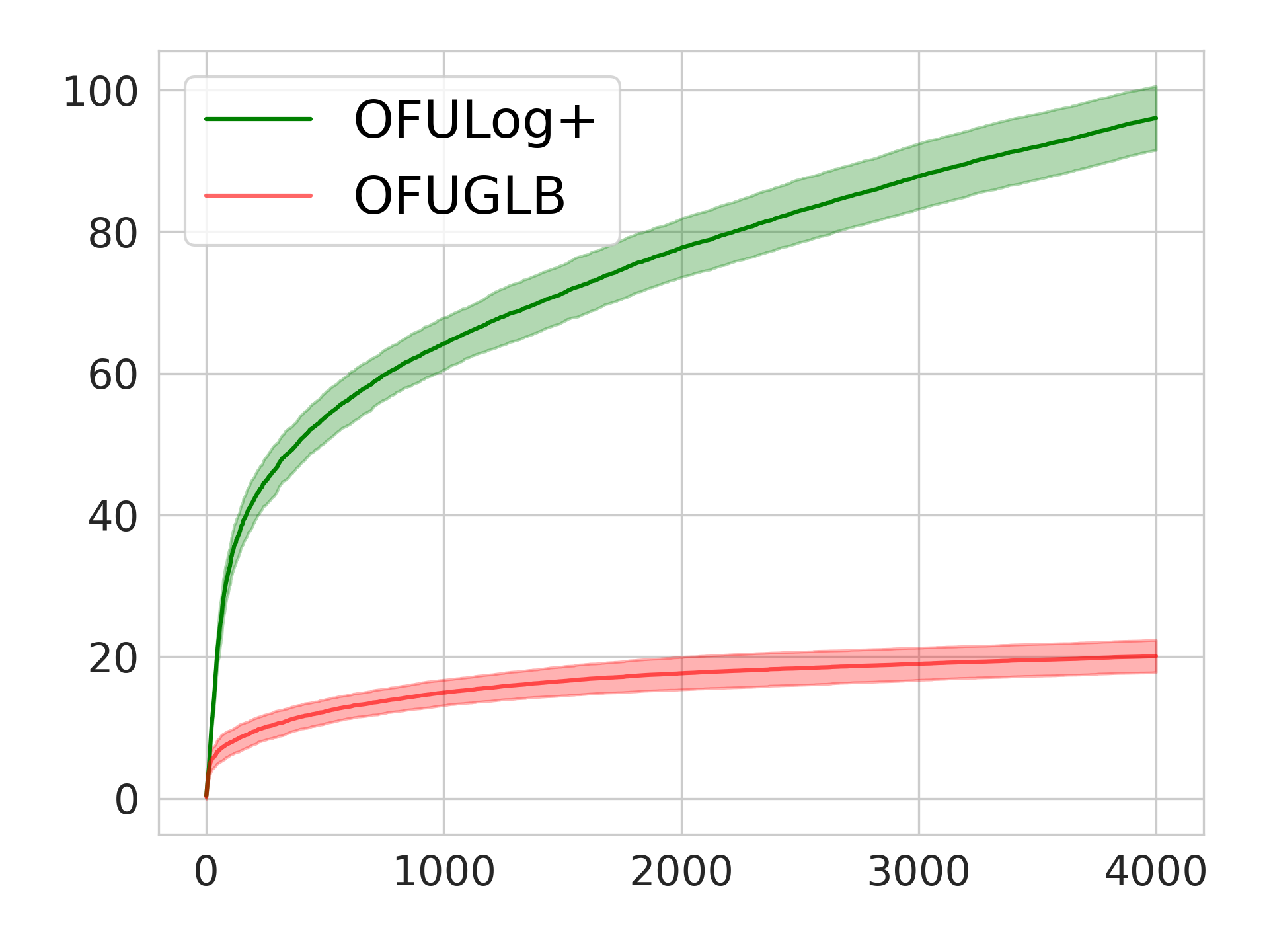
(a) $S=5$

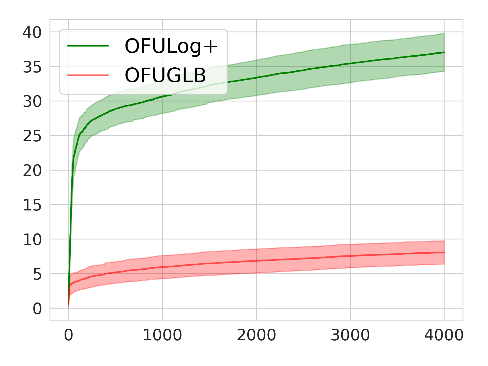
(b) $S=10$

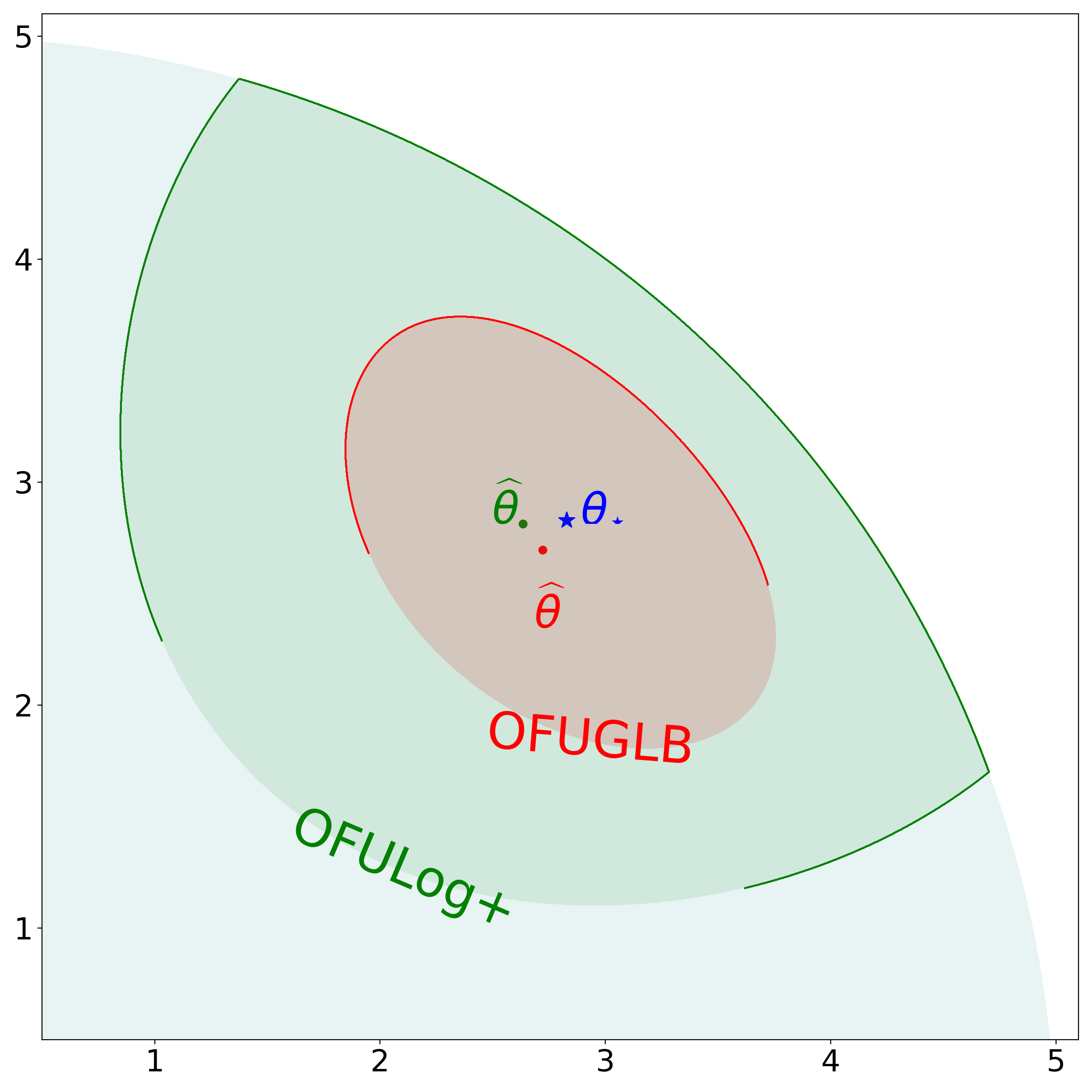
(c) $S=5$

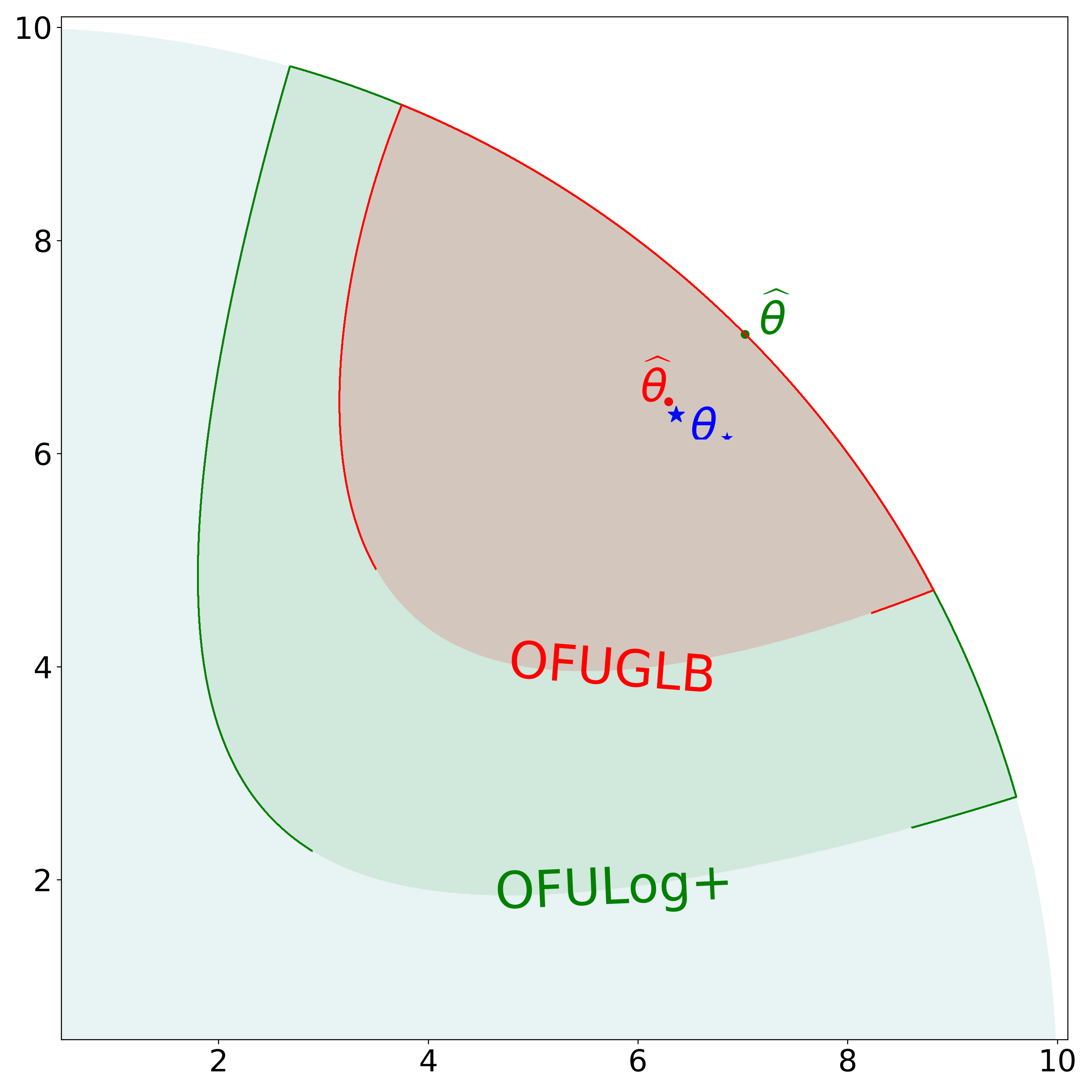
(d) $S=10$

Figure 1: (a,b) Regret plots for considered algorithms. (c,d) Confidence sets at $t=4000$ from a single run: red is from OFUGLB and green is from OFULog+.

Experiments for Logistic Bandits.

To complement the improvement in our regret bounds and CS, we perform experiments on logistic bandits by comparing our OFUGLB to OFULog+ (Lee et al., 2024). Following the setting of Lee et al. (2024), for OFUGLB and OFULog+, we utilize Sequential Least SQuares Programming (SLSQP) implemented in SciPy (Virtanen et al., 2020) for precise computation of the norm-constrained MLE at each time step for a fairer comparison. For the parameters, we set $T=4000$, $d=2$, $|{\mathcal{A}}|=20$, and $\delta=0.05$, and we average over $10$ independent random trials for the regret comparison. We use ${\color[rgb]{0,0,1}\bm{\theta}_{\star}}=\frac{S-1}{\sqrt{d}}\bm{1}$ for $S\in\{5,10\}$, and time-varying arm-set by sampling in the unit ball at random at each $t$. The regret curves shown in Figure 1(a) and 1(b) clearly show that OFUGLB numerically outperforms OFULog+. The confidence sets at $t=4000$ shown in Figure 1(c) and 1(d) indicates that, indeed, our confidence set from Theorem 3.1 is much smaller than that of Lee et al. (2024), which shows the practical benefit of our novel CS.

Poisson Bandits.

Despite its potential to model various real-world problems involving count feedback, Poisson bandits have not been studied often in the literature. Gisselbrecht et al. (2015) was the first to consider contextual Poisson bandits and proposed UCB and optimistic Bayesian-based algorithms (May et al., 2012), but without any regret guarantees. To our knowledge, this is the first regret bound for the (finite-dimensional) contextual Poisson bandits without reward boundedness assumption. On a related note, Mutný and Krause (2021) consider Poisson bandits with the intensity function in an RKHS. Their linear RKHS formulation is, however, incompatible with our log-linear formulation; see their Appendix A.1 for further discussions.

5 Conclusion and Future Work

This paper introduces a novel and unified likelihood ratio-based CS for generic (convex) GLMs, encompassing widely-used models such as Gaussian, Bernoulli, and Poisson. Especially for Bernoulli, this leads to the first $\operatorname{poly}(S)$-free CS, resolving an open problem posed in Lee et al. (2024). Our CS is equipped with exact constants for various scenarios, making it suitable for any practitioner to use. The proof involves leveraging key techniques from PAC-Bayes bounds along with a uniform prior/posterior, which may be of independent interest. We then propose OFUGLB, a generic UCB algorithm applicable to any GLBs, achieving state-of-the-art regret bounds across various instantiations (linear, logistic, GLM). The proof involves novel regret decomposition and maximally avoiding the self-concordance control lemma (Faury et al., 2020, Lemma 9), which may also be of independent interest. Notably, for logistic bandits, OFUGLB is the first pure-optimism-based algorithm that achieves $\operatorname{poly}(S)$-free leading term in the theoretical regret and is numerically verified to be the best.

This work opens up various future directions, some of which we discuss here. One is to extend our results to kernelized or functional GLM (Cawley et al., 2007; Müller and Stadtmüller, 2005), which would be an interesting nonlinear generalization of the linear kernel bandits (Chowdhury and Gopalan, 2017; Srinivas et al., 2010). The optimality of our obtained CS radius (Duchi and Haque, 2024) as well as the leading term in the regret of GLB (Abeille et al., 2021), especially with respect to $S$, is an important question. It would be interesting to see if our new CS leads to any improvements in the best arm identification of GLBs from our new CS (Kazerouni and Wein, 2021; Jun et al., 2021; Azizi et al., 2022) and even sample-efficient RLHF (Das et al., 2024; Shi et al., 2024).

Appendix A Missing Results and Proofs

A.1 Bounding $L_{t}$ for Gaussian Distribution

We first recall some definitions:

Definition A.1.

A random variable $X\in{\mathbb{R}}$ is $\sigma$-subGaussian, if ${\mathbb{P}}(\left|X-\mathbb{E}[X]\right|\geq t)\leq 2\exp\left(-\frac{t^{2}}{2\sigma^{2}}\right),\ \forall t\in{\mathbb{R}}$.

Definition A.2 (Definition 3 of Jin et al. (2019)).

A random vector ${\bm{X}}\in{\mathbb{R}}^{d}$ is $\sigma$-norm-subGaussian, if ${\mathbb{P}}(\left\lVert{\bm{X}}-\mathbb{E}[{\bm{X}}]\right\rVert_{2}\geq t)\leq 2\exp\left(-\frac{t^{2}}{2\sigma^{2}}\right),\ \forall t\in{\mathbb{R}}$.

Here is the full statement:

Proposition A.1.

Suppose the GLM is $\sigma$-subGaussian. Then, for any $\delta\in(0,1)$,

$${\mathbb{P}}\left(\exists t\geq 1\mathrel{\mathop{\mathchar 58\relax}}L_{t}>\frac{2}{g(\tau)}\left(R_{\dot{\mu}}S(t-1)+2\pi\sigma\sqrt{(t-1)\log\frac{\pi^{2}dt^{2}}{3\delta}}\right)\right)\leq\delta.$$ (13)

Proof.

Here, as $\max_{{\bm{x}}\in{\mathcal{X}},\bm{\theta}\in\Theta}|\dot{\mu}(\langle{\bm{x}},\bm{\theta}\rangle)|\leq R_{\dot{\mu}}$, we have that

$$L_{t} =\frac{1}{g(\tau)}\max_{\bm{\theta}\in\Theta}\left\lVert\sum_{s=1}^{t-1}(r_{s}-\mu(\langle{\bm{x}}_{s},\bm{\theta}\rangle)){\bm{x}}_{s}\right\rVert_{2}$$

$$\leq\frac{1}{g(\tau)}\max_{\bm{\theta}\in\Theta}\left\lVert\sum_{s=1}^{t-1}(\mu(\langle{\bm{x}}_{s},\bm{\theta}\rangle)-\mu(\langle{\bm{x}}_{s},\bm{\theta}_{\star}\rangle)){\bm{x}}_{s}\right\rVert_{2}+\frac{1}{g(\tau)}\left\lVert\sum_{s=1}^{t-1}\underbrace{(r_{s}-\mu(\langle{\bm{x}}_{s},\bm{\theta}_{\star}\rangle)){\bm{x}}_{s}}_{\triangleq{\bm{y}}_{s}}\right\rVert_{2}$$

$$\leq\frac{2R_{\dot{\mu}}S(t-1)}{g(\tau)}+\frac{1}{g(\tau)}\left\lVert\sum_{s=1}^{t-1}{\bm{y}}_{s}\right\rVert_{2}.$$

We now utilize subGaussian concentrations from Jin et al. (2019). First note that ${\bm{y}}_{s}$ is a martingale difference sequence adapted to $\Sigma_{s}$ and is norm-subGaussian with (conditional) variance $\sigma^{2}$ be given. Then, by Corollary 7 of Jin et al. (2019), we have that

$${\mathbb{P}}\left(\left\lVert\sum_{s=1}^{t-1}{\bm{y}}_{s}\right\rVert_{2}\leq 4\pi\sigma\sqrt{(t-1)\log\frac{2d}{\delta}}\right)\geq 1-\delta,\quad\forall t\geq 1.$$ (14)

The exact constant $4\pi$ is not available in Jin et al. (2019), as all the constants are hidden under $c$. This is not useful, especially for practitioners wanting to use the concentration directly. Thus, we tracked the constant from their Corollary 7, the details of which we provide in Lemma A.1.

We then conclude by parametrizing $\delta$ as $\delta/t^{2}$, applying union bound over $t\geq 1$, and using the Basel sum. ∎

Lemma A.1 (Lemma 2 of Jin et al. (2019); originally Lemma 5.5 of Vershynin (2010)).

For any $\sigma$-norm-subGaussian random vector ${\bm{X}}$, we have that $\sup_{p\in{\mathbb{N}}}p^{-1/2}\left(\mathbb{E}[\left\lVert{\bm{X}}\right\rVert^{p}]\right)^{1/p}\leq\sqrt{\pi}\sigma$.

Proof.

This follows from brute-force computation. First, we have that

$$\mathbb{E}[\left\lVert{\bm{X}}\right\rVert^{p}]=\int_{0}^{\infty}{\mathbb{P}}[\left\lVert{\bm{X}}\right\rVert^{p}\geq t]dt=p\int_{0}^{\infty}{\mathbb{P}}[\left\lVert{\bm{X}}\right\rVert\geq t]t^{p-1}dt \leq 2p\int_{0}^{\infty}t^{p-1}\exp\left(-\frac{t^{2}}{2\sigma^{2}}\right)dt$$

$$=2^{\frac{p-1}{2}}\sigma^{p}p\Gamma\left(\frac{p}{2}\right).$$

Then, for any $p\in{\mathbb{N}}$,

$$p^{-1/2}(\mathbb{E}[\left\lVert{\bm{X}}\right\rVert^{p}])^{1/p}=\sigma 2^{\frac{p-1}{2p}}p^{\frac{1}{p}-\frac{1}{2}}\left(\sqrt{\pi}\frac{(p-2)!!}{2^{\frac{p-1}{2}}}\right)^{1/p}=\sigma\underbrace{p^{\frac{1}{p}-\frac{1}{2}}\left(\sqrt{\pi}(p-2)!!\right)^{1/p}}_{\triangleq f(p)}.$$

Using WolframAlpha, we can conclude that $f(p)$ is decreasing, and we conclude by noting that $f(1)=\sqrt{\pi}$. ∎

A.2 Bounding $L_{t}$ for Poisson Distribution

We have the following result for Poisson, which may be of independent interest (to our knowledge, this is the first explicit martingale concentration for Poisson):

Proposition A.2.

For the Poisson distribution, we have that for any $\delta\in(0,1)$: when $S>1$,

$${\mathbb{P}}\left(L_{t}\leq C(S)(t-1)+\frac{2}{1-2e^{-S}}\log\frac{\pi^{2}(d+1)t^{2}}{3\delta}\right)\geq 1-\delta,\quad\forall t\geq 1,$$ (15)

where $C(S)\mathrel{\mathop{\mathchar 58\relax}}=\frac{1}{4}(1-2e^{-S})(e^{S}+2S+2\log\frac{2(1-2e^{-S})}{e})+2Se^{S}$. When $S\leq 1$,

$${\mathbb{P}}\left(L_{t}\leq\tilde{C}(S)(t-1)+4\log\frac{\pi^{2}(d+1)t^{2}}{3\delta}\right)\geq 1-\delta,\quad\forall t\geq 1,$$ (16)

where $\tilde{C}(S)\mathrel{\mathop{\mathchar 58\relax}}=\frac{1}{16}\left(e^{S}+4S+4\log(8+2e^{S})\right)+2Se^{S}$.

Proof.

Proceeding similarly as in the previous subsection, we first have that

$$L_{t}\leq 2Se^{S}(t-1)+\left\lVert\sum_{s=1}^{t-1}{\bm{y}}_{s}\right\rVert_{2},$$ (17)

where ${\bm{y}}_{s}=(r_{s}-e^{\langle{\bm{x}}_{s},\bm{\theta}_{\star}\rangle}){\bm{x}}_{s}$ is the martingale difference sequence satisfying $\mathbb{E}[{\bm{y}}_{s}|\Sigma_{s}]={\bm{0}}$ as $r_{s}|\Sigma_{s}\sim\mathrm{Poi}(\langle{\bm{x}}_{s},\bm{\theta}_{\star}\rangle)$.

We now modify the proof of Corollary 7 of Jin et al. (2019) (which is based upon the celebrated Chernoff-Cramér method) for the Poisson martingale vectors, details of which we provide here for completeness.

First, we consider the following MGF bound of the Poisson distribution whose proof is deferred to the end of this subsection:

Lemma A.2.

Suppose that the random vector ${\bm{y}}$ is of the form ${\bm{y}}=(r-\lambda){\bm{x}}$ for some fixed ${\bm{x}}\in{\mathcal{B}}^{d}(1)$, $r\sim\mathrm{Poi}(\lambda)$, and $\lambda>0$. Then, for the Hermitian dilation (Tropp, 2015, Definition 2.1.5) of ${\bm{y}}$, ${\bm{Y}}\mathrel{\mathop{\mathchar 58\relax}}=\begin{bmatrix}0&{\bm{y}}^{\top}\\ {\bm{y}}&{\bm{0}}\end{bmatrix}$, we have that $\mathbb{E}e^{\theta{\bm{Y}}}\preceq\exp\left(F(\theta,\lambda)\right){\bm{I}}_{d+1}$ for $|\theta|<\frac{1}{2}$, where $F(\theta,\lambda)\mathrel{\mathop{\mathchar 58\relax}}=\lambda|\theta|+\log(2|\theta|)+\log\left(\frac{e^{-\frac{\lambda}{2}}}{\frac{1}{2}-|\theta|}+\lambda\right)$.

We also recall the Lieb’s trace inequality:

Theorem A.3 (Theorem 6 of Lieb (1973)).

Let ${\bm{A}}$ be a fixed symmetric matrix, and let ${\bm{Y}}$ be a random symmetric matrix. Then,

$$\mathbb{E}\operatorname{\mathrm{tr}}(\exp({\bm{A}}+{\bm{Y}}))\leq\operatorname{\mathrm{tr}}\exp({\bm{A}}+\log\mathbb{E}e^{\bm{Y}})$$ (18)

Now let $0<\theta<\frac{1}{2}$ be fixed, and let us denote $\lambda_{s}\mathrel{\mathop{\mathchar 58\relax}}=e^{\langle{\bm{x}}_{s},\bm{\theta}_{\star}\rangle}$ and $\mathbb{E}_{s}[\cdot]\mathrel{\mathop{\mathchar 58\relax}}=\mathbb{E}[\cdot|\Sigma_{s}]$ for $s\leq t-1$. We start by noting that

$$\mathbb{E}\operatorname{\mathrm{tr}}\exp\left(-\theta^{2}{\bm{I}}_{d+1}\sum_{s=1}^{t-1}F(\theta,\lambda_{s})+\theta\sum_{s=1}^{t-1}{\bm{Y}}_{s}\right)$$

$$=\mathbb{E}\left[\mathbb{E}_{t-1}\left[\operatorname{\mathrm{tr}}\exp\left(-\theta^{2}{\bm{I}}_{d+1}\sum_{s=1}^{t-1}F(\theta,\lambda_{s})+\theta\sum_{s=1}^{t-1}{\bm{Y}}_{s}\right)\right]\right]$$

$$\leq\mathbb{E}\left[\operatorname{\mathrm{tr}}\exp\left(-\theta^{2}{\bm{I}}_{d+1}\sum_{s=1}^{t-1}F(\theta,\lambda_{s})+\theta\sum_{s=1}^{t-2}{\bm{Y}}_{s}+\log\mathbb{E}_{t-1}\left[e^{\theta{\bm{Y}}_{t-1}}\right]\right)\right]$$ (Theorem A.3)

$$\leq\mathbb{E}\left[\operatorname{\mathrm{tr}}\exp\left(-\theta^{2}{\bm{I}}_{d+1}\sum_{s=1}^{t-1}F(\theta,\lambda_{s})+\theta\sum_{s=1}^{t-2}{\bm{Y}}_{s}+F(\theta,\lambda_{t-1}){\bm{I}}_{d+1}\right)\right] {\bm{A}}\preceq{\bm{B}}\Rightarrow e^{{\bm{C}}+{\bm{A}}}\preceq e^{{\bm{C}}+{\bm{B}}}$$ (Lemma A.2, )

$$\leq\mathbb{E}\left[\operatorname{\mathrm{tr}}\exp\left(-\theta^{2}{\bm{I}}_{d+1}\sum_{s=1}^{t-2}F(\theta,\lambda_{s})+\theta\sum_{s=1}^{t-2}{\bm{Y}}_{s}\right)\right]$$

$$\leq\cdots\leq\operatorname{\mathrm{tr}}\exp(0{\bm{I}}_{d+1})=d+1.$$

Thus, for any $\rho\geq 0$,

$${\mathbb{P}}\left(\left\lVert\sum_{s=1}^{t-1}{\bm{y}}_{s}\right\rVert\geq\theta\sum_{s=1}^{t-1}F(\theta,\lambda_{s})+\frac{\rho}{\theta}\right)$$

$$={\mathbb{P}}\left(\left\lVert\sum_{s=1}^{t-1}{\bm{Y}}_{s}\right\rVert\geq\theta\sum_{s=1}^{t-1}F(\theta,\lambda_{s})+\frac{\rho}{\theta}\right) \sum_{s}{\bm{Y}}_{s} \pm\left\lVert\sum_{s}{\bm{y}}_{s}\right\rVert_{2}$$ ( is a rank-2 matrix with eigenvalues )

$$=2{\mathbb{P}}\left(\lambda_{\max}\left(\sum_{s=1}^{t-1}{\bm{Y}}_{s}\right)\geq\theta\sum_{s=1}^{t-1}F(\theta,\lambda_{s})+\frac{\rho}{\theta}\right) {\bm{Y}}_{s}$$ (’s are symmetric)

$$=2{\mathbb{P}}\left(\lambda_{\max}\left(\exp\left(\theta\sum_{s=1}^{t-1}{\bm{Y}}_{s}\right)\right)\geq\exp\left(\theta^{2}\sum_{s=1}^{t-1}F(\theta,\lambda_{s})+\rho\right)\right)$$

$$\leq 2{\mathbb{P}}\left(\operatorname{\mathrm{tr}}\exp\left(\theta\sum_{s=1}^{t-1}{\bm{Y}}_{s}\right)\geq\exp\left(\theta^{2}\sum_{s=1}^{t-1}F(\theta,\lambda_{s})+\rho\right)\right)$$

$$\leq 2e^{-\rho}\mathbb{E}\operatorname{\mathrm{tr}}\exp\left(-\theta^{2}\sum_{s=1}^{t-1}F(\theta,\lambda_{s})+\theta\sum_{s=1}^{t-1}{\bm{Y}}_{s}\right)$$ (Markov’s inequality)

$$\leq 2(d+1)e^{-\rho}.$$ (Lemma A.2)

Finally, by reparametrizing, we have that for any $\delta\in(0,1)$,

$${\mathbb{P}}\left(\left\lVert\sum_{s=1}^{t-1}{\bm{y}}_{s}\right\rVert\geq\inf_{\theta\in(0,1/2)}\left\{\theta\sum_{s=1}^{t-1}F(\theta,\lambda_{s})+\frac{1}{\theta}\log\frac{2d}{\delta}\right\}\right)\leq\delta,$$ (19)

where we recall that $F(\theta,\lambda)=\lambda\theta+\log(2\theta)+\log\left(\frac{e^{-\frac{\lambda}{2}}}{\frac{1}{2}-\theta}+\lambda\right)$ for $\theta>0$.

First, when $S>1$, let us choose $\theta=\frac{1}{2}-e^{-S}$, which is guaranteed to be positive. Noting that $\lambda_{s}=e^{\langle{\bm{x}}_{s},\bm{\theta}_{\star}\rangle}\leq e^{S}$, we have

$$F\left(\frac{1}{2}-e^{-S},\lambda_{s}\right)\leq e^{S}\left(\frac{1}{2}-e^{-S}\right)+\log(1-2e^{-S})+\log(2e^{S})=\frac{1}{2}e^{S}+S+\log\frac{2(1-2e^{-S})}{e}.$$

Thus, the RHS of Eqn. (19)

$$\frac{(1-2e^{-S})(e^{S}+2S+2\log\frac{2(1-2e^{-S})}{e})}{4}(t-1)+\frac{2}{1-2e^{-S}}\log\frac{2(d+1)}{\delta}.$$ (20)

For the case $S\leq 1$, choosing $\theta=\frac{1}{4}$, the RHS becomes

$$\frac{e^{S}+4S+4\log(8+2e^{S})}{16}(t-1)+4\log\frac{2(d+1)}{\delta}.$$ (21)

Finally, we conclude by parametrizing $\delta$ as $\delta/t^{2}$, applying union bound over $t\geq 1$, and using the Basel sum. ∎

Proof of Lemma A.2.

We first have that

$$\mathbb{E}e^{\theta{\bm{Y}}}\overset{(*)}{=}{\bm{I}}_{d+1}+\sum_{p=1}^{\infty}\frac{\theta^{p}\mathbb{E}{\bm{Y}}^{2p}}{(2p)!}\preceq{\bm{I}}_{d+1}+\sum_{p=1}^{\infty}\frac{\theta^{2p}\mathbb{E}\left\lVert{\bm{y}}\right\rVert^{2p}}{(2p)!}{\bm{I}}_{d+1} =\mathbb{E}\left[\frac{e^{\theta\left\lVert{\bm{y}}\right\rVert}+e^{-\theta\left\lVert{\bm{y}}\right\rVert}}{2}\right]{\bm{I}}_{d+1}$$

$$\preceq\mathbb{E}\left[e^{|\theta||r-\lambda|}\right]{\bm{I}}_{d+1},$$

where $(*)$ follows from the observation that $\mathbb{E}{\bm{Y}}^{2p+1}={\bm{0}}$. We now recall a well-known concentration for Poisson distribution (taken from a note by C. Canonne):

Lemma A.3.

${\mathbb{P}}(|r-y|\geq x)\leq 2e^{-\frac{x^{2}}{2(\lambda+x)}}$.

Then, we have that

$$\mathbb{E}[e^{|\theta||r-\lambda|}] =\int_{0}^{\infty}{\mathbb{P}}(e^{|\theta||r-\lambda|}>k)dk dk$$ ( is the Lebesgue measure)

$$\leq 1+\int_{1}^{\infty}{\mathbb{P}}(e^{|\theta||r-\lambda|}\geq k)dk$$

$$\leq 2\int_{1}^{\infty}e^{-\frac{(\log k/|\theta|)^{2}}{2(\lambda+\log k/|\theta|)}}dk$$ (Lemma A.3)

$$=2|\theta|\int_{0}^{\infty}e^{-\frac{u^{2}}{2(\lambda+u)}+|\theta|u}du$$

$$=2|\theta|\left\{\int_{\lambda}^{\infty}e^{-\frac{u^{2}}{2(\lambda+u)}+|\theta|u}du+\int_{0}^{\lambda}e^{-\frac{u^{2}}{2(\lambda+u)}+|\theta|u}du\right\}$$

$$\leq 2|\theta|\left\{\int_{\lambda}^{\infty}e^{-(\frac{1}{2}-|\theta|)u}du+\lambda e^{|\theta|\lambda}\right\} \frac{u^{2}}{2(\lambda+u)}\geq\frac{1}{2}u u\geq\lambda$$ ( for )

$$\leq 2|\theta|\left(\frac{1}{\frac{1}{2}-|\theta|}e^{-(\frac{1}{2}-|\theta|)\lambda}+\lambda e^{|\theta|\lambda}\right)$$

$$=\exp\left(F(\theta,\lambda)\triangleq\lambda|\theta|+\log(2|\theta|)+\log\left(\frac{e^{-\frac{\lambda}{2}}}{\frac{1}{2}-|\theta|}+\lambda\right)\right).$$

∎

A.3 Proof of Theorem 3.2 – Ellipsoidal Confidence Sequence

First, similarly to prior works on logistic bandits (Abeille et al., 2021; Lee et al., 2024), let us define the following quantities:

$$\widetilde{{\bm{G}}}_{t}(\bm{\theta},\bm{\nu})\mathrel{\mathop{\mathchar 58\relax}}=\frac{1}{g(\tau)}\sum_{s=1}^{t-1}\tilde{\alpha}_{s}(\bm{\theta},\bm{\nu}){\bm{x}}_{s}{\bm{x}}_{s}^{\top},\ \tilde{\alpha}_{s}(\bm{\theta},\bm{\nu})\mathrel{\mathop{\mathchar 58\relax}}=\int_{0}^{1}(1-v)\dot{\mu}\left(\langle{\bm{x}}_{s},\bm{\theta}+v(\bm{\nu}-\bm{\theta})\rangle\right)dv.$$

(We will later come back to these quantities in the regret analysis.)

Then, by Taylor’s theorem with integral remainder, we have that for any $\lambda\geq 0$ to be chosen later,

$$\beta_{t}(\delta)^{2}\geq{\mathcal{L}}_{t}(\bm{\theta})-{\mathcal{L}}_{t}(\widehat{\bm{\theta}}_{t}) =\underbrace{\langle\nabla{\mathcal{L}}_{t}(\widehat{\bm{\theta}}_{t}),\bm{\theta}-\widehat{\bm{\theta}}_{t}\rangle}_{=0}+\left\lVert\bm{\theta}-\widehat{\bm{\theta}}_{t}\right\rVert_{\widetilde{{\bm{G}}}_{t}(\widehat{\bm{\theta}}_{t},\bm{\theta})}^{2}$$

$$=\left\lVert\bm{\theta}-\widehat{\bm{\theta}}_{t}\right\rVert_{\widetilde{{\bm{G}}}_{t}(\widehat{\bm{\theta}}_{t},\bm{\theta})+\lambda{\bm{I}}_{d}}^{2}-\lambda\left\lVert\bm{\theta}-\widehat{\bm{\theta}}_{t}\right\rVert_{2}^{2}$$

$$\geq\left\lVert\bm{\theta}-\widehat{\bm{\theta}}_{t}\right\rVert_{\widetilde{{\bm{G}}}_{t}(\widehat{\bm{\theta}}_{t},\bm{\theta})+\lambda{\bm{I}}_{d}}^{2}-4S^{2}\lambda.$$

We conclude by choosing $\lambda=\frac{1}{4S^{2}}$ and the self-concordance control for $\widetilde{{\bm{G}}}$ (Abeille et al., 2021, Lemma 8), which we recall here:

Lemma A.4 (A slight extension of Lemma 8 of Abeille et al. (2021)).

Let $\mu$ be increasing ($\dot{\mu}\geq 0$, which is basically Assumption 3) and self-concordant with constant $R_{s}$ (as in Assumption 4). Let ${\mathcal{Z}}\subset{\mathbb{R}}$ be bounded. Then, the following holds for any $z_{1},z_{2}\in{\mathcal{Z}}$:

$$\int_{0}^{1}(1-v)\dot{\mu}(z_{1}+v(z_{2}-z_{1}))dv\geq\frac{\dot{\mu}(z_{1})}{2+R_{s}|z_{1}-z_{2}|}.$$

This then implies that $\widetilde{{\bm{G}}}_{t}(\bm{\theta},\bm{\nu})\succeq\frac{1}{2+2SR_{s}}\nabla^{2}{\mathcal{L}}_{t}(\bm{\theta})$.

Appendix B Proof of Theorem 4.1 – Regret Bound of OFUGLB

B.1 Key Ideas of the Proof

Why Prior Proof Technique Fails.

The prior proof technique of Abeille et al. (2021) first bounds the regret by $\sum_{t=1}^{T}{\dot{\mu}}_{t}({\bm{\theta}}_{\star}){\bm{x}}_{t}^{\top}({\bm{\theta}}_{t}-{\bm{\theta}}_{\star})$, where ${\dot{\mu}}_{t}({\bm{\theta}})\mathrel{\mathop{\mathchar 58\relax}}={\dot{\mu}}({\bm{x}}_{t}^{\top}{\bm{\theta}})$, plus a lower order term that is easy to control. Denoting $H_{t}(\bm{\theta}_{\star})\mathrel{\mathop{\mathchar 58\relax}}=\lambda{\bm{I}}+\nabla^{2}{\mathcal{L}}_{t}(\bm{\theta}_{\star})$, they use Cauchy-Schwarz to obtain

$${\dot{\mu}}_{t}({\bm{\theta}}_{\star}){\bm{x}}_{t}^{\top}({\bm{\theta}}_{t}-{\bm{\theta}}_{\star})\leq{\dot{\mu}}_{t}({\bm{\theta}}_{\star})\mathinner{\|{\bm{x}}_{t}\|}_{H_{t}({\bm{\theta}}_{\star})^{-1}}(\mathinner{\|{\bm{\theta}}_{t}-\widehat{\bm{\theta}}_{t}\|}_{H_{t}({\bm{\theta}}_{\star})}+\mathinner{\|{\bm{\theta}}_{\star}-\widehat{\bm{\theta}}_{t}\|}_{H_{t}({\bm{\theta}}_{\star})}).$$

They then use Taylor expansion and self-concordant control (Abeille et al., 2021, Lemma 8) to obtain $\mathinner{\|{\bm{\theta}}_{t}-\widehat{\bm{\theta}}_{t}\|}_{H_{t}({\bm{\theta}}_{\star})}={\mathcal{O}}\left(S\beta_{t}(\delta)\right)$ from the likelihood-based confidence set ${\mathcal{L}}_{t}(\bm{\theta}_{t})-{\mathcal{L}}_{t}(\widehat{\bm{\theta}}_{t})\leq\beta_{t}(\delta)^{2}$, which introduces a factor of $S$. Thus, even if $\beta_{t}(\delta)$ is $\mathrm{poly}(S)$-free, following this proof still results in a regret whose leading term is not $\operatorname{poly}(S)$-free.

Our Approach.

We instead use Cauchy-Schwartz with respect to a difference matrix $\widetilde{{\bm{G}}}_{t}$, which satisfies $\mathinner{\|{\bm{\theta}}_{t}-\widehat{\bm{\theta}}_{t}\|}_{{\widetilde{{\bm{G}}}}_{t}}={\mathcal{O}}(\beta_{t}(\delta))$. We avoid the extra $S$ compared to the prior approach that uses Cauchy-Schwartz w.r.t. ${\bm{H}}_{t}$. However, the main difficulty of the proof is that $\widetilde{{\bm{G}}}_{t}$ is not in a suitable form for elliptical potential arguments. To see this clearly, consider the following natural optimistic upper-bound of the instantaneous regret:

$$\mu(\langle{\bm{x}}_{t,\star},{\bm{\theta}}_{\star}\rangle)-\mu_{t}({\bm{\theta}}_{\star}) \leq\mu_{t}({\bm{\theta}}_{t})-\mu_{t}({\bm{\theta}}_{\star})$$ (Optimism)

$$=\mu_{t}({\bm{\theta}}_{t})-\mu_{t}(\widehat{\bm{\theta}}_{t})-\mu_{t}(\widehat{\bm{\theta}}_{t})+\mu_{t}({\bm{\theta}}_{\star})$$

$$\leq 2|\mu_{t}({\bm{\theta}}^{\prime}_{t})-\mu_{t}(\widehat{\bm{\theta}}_{t})|$$

$$\lesssim{\dot{\mu}}_{t}(\widehat{\bm{\theta}}_{t})|\langle{\bm{x}}_{t},{\bm{\theta}}^{\prime}_{t}-\widehat{\bm{\theta}}_{t}\rangle|+\text{lower order terms},$$ (Taylor’s theorem)

where ${\bm{\theta}}^{\prime}_{t}=\arg\max_{{\bm{\theta}}\in\mathcal{C}_{t}}|\mu_{t}({\bm{\theta}})-\mu_{t}(\widehat{\bm{\theta}}_{t})|$. One can then apply the aforementioned Cauchy-Schwarz w.r.t. $\widetilde{{\bm{G}}}_{t}$ to obtain

$${\dot{\mu}}_{t}(\widehat{\bm{\theta}}_{t})|\langle{\bm{x}}_{t},{\bm{\theta}}^{\prime}_{t}-\widehat{\bm{\theta}}_{t}\rangle|\leq{\dot{\mu}}_{t}(\widehat{\bm{\theta}}_{t})\mathinner{\|{\bm{x}}_{t}\|}_{\widetilde{{\bm{G}}}_{t}^{-1}}\mathinner{\|{\bm{\theta}}_{t}-\widehat{\bm{\theta}}_{t}\|}_{\widetilde{{\bm{G}}}_{t}}\leq{\dot{\mu}}_{t}(\widehat{\bm{\theta}}_{t})\mathinner{\|{\bm{x}}_{t}\|}_{\widetilde{{\bm{G}}}_{t}^{-1}}\cdot O(\beta_{T}(\delta)).$$

This successfully avoids using previous self-concordant control (Abeille et al., 2021, Lemma 8), and thus seemingly getting closer to obtaining a $\operatorname{poly}(S)$-free regret. Omitting details, the final step is to sum the above over $t\in[T]$ and apply the elliptical potential lemma (EPL; Abbasi-Yadkori et al. (2011)). But, this is not possible, as we can only apply the EPL when ${\widetilde{{\bm{G}}}}_{t}$ can be written as $\lambda{\bm{I}}+\sum_{s=1}^{t-1}{\dot{\mu}}_{s}(\widehat{\bm{\theta}}_{s}){\bm{x}}_{s}{\bm{x}}_{s}^{\top}$ for some $\lambda>0$, and ${\widetilde{{\bm{G}}}}_{t}$ depends on ${\bm{\theta}}_{t}$ and not on $\widehat{\bm{\theta}}_{s}$ for $s\in[t-1]$. The most challenging part of our proof development is making EPL applicable to the summation resulting from some decomposition of the (instantaneous) regret while avoiding extra $S$-dependencies.

The key insight is that if we could designate a “worst-case” ${\overline{{\bm{\theta}}}}_{s}$ for each time step $s$ such that ${\widetilde{{\bm{G}}}}_{t}\succeq\lambda I+\sum_{s=1}^{t-1}{\dot{\mu}}({\overline{{\bm{\theta}}}}_{s})x_{s}x_{s}^{\top}=\mathrel{\mathop{\mathchar 58\relax}}{\bm{Q}}_{t}$, then we can perform the following:

$${\dot{\mu}}_{t}(\widehat{\bm{\theta}}_{t})|\langle{\bm{x}}_{t},{\bm{\theta}}^{\prime}_{t}-\widehat{\bm{\theta}}_{t}\rangle|\leq{\dot{\mu}}_{t}({\overline{{\bm{\theta}}}}_{t})|\langle{\bm{x}}_{t},{\bm{\theta}}^{\prime}_{t}-\widehat{\bm{\theta}}_{t}\rangle|+|{\dot{\mu}}_{t}(\widehat{\bm{\theta}}_{t})-{\dot{\mu}}_{t}({\overline{{\bm{\theta}}}}_{t})||\langle{\bm{x}}_{t},{\bm{\theta}}^{\prime}_{t}-\widehat{\bm{\theta}}_{t}\rangle|$$

where the first term is now be bounded by ${\dot{\mu}}_{t}({\overline{{\bm{\theta}}}}_{t})\mathinner{\!\left\|{\bm{x}}_{t}\right\|}_{{\bm{Q}}_{t}^{-1}}\cdot{\mathcal{O}}(\beta_{T}(\delta))$. We can now apply the EPL when summing over $t\in[T]$, thanks to the form of ${\bm{Q}}_{t}$. The second term turns out to be a lower order term via our new self-concordant control that doesn’t give additional $S$-dependency (Lemma B.3).

However, designating such ${\overline{{\bm{\theta}}}}_{s}$ seems nontrivial from the proof structure above for a technical reason. Initially, we were able to resolve it by using a confidence set defined as an intersection over all the confidence sets used so far, or by using an additional constraint set $\mathcal{W}_{t}$ as defined in Logistic-UCB-2 of Faury et al. (2020). However, either approach significantly increases the computational complexity.

We later discovered that we could resolve the issue without changing the confidence set through an alternate analysis, which is the current proof. Specifically, we consider the following decomposition of the instantaneous regret:

$$\mu(\langle{\bm{x}}_{t,\star},{\bm{\theta}}_{\star}\rangle)-\mu_{t}({\bm{\theta}}_{\star})\leq\mu_{t}({\bm{\theta}}_{t})-\mu_{t}({\bm{\theta}}_{\star})\leq 2|\mu_{t}(\bm{\nu}_{t})-\mu_{t}(\widehat{\bm{\theta}}_{b(t)})|,$$

where we define $(b(t),\bm{\nu}_{t})=\arg\max_{b\in[t,T],{\bm{\theta}}\in\mathcal{C}_{b}}|\mu_{t}({\bm{\theta}})-\mu_{t}(\widehat{\bm{\theta}}_{b})|$. That is, we are bounding the instantaneous regret by how large the difference can be from the current confidence set and how large the difference can be from the future confidence sets. With this, we can then define $\bar{\bm{\theta}}_{t}\mathrel{\mathop{\mathchar 58\relax}}=\operatorname*{arg\,min}_{\bm{\theta}\in\bigcup_{b\in[t,T]}{\mathcal{C}}_{b}}\dot{\mu}_{t}(\bm{\theta}),$ which satisfies the aforementioned desired property.

Among the omitted details, we consider a slightly more intricate regret decomposition by considering timesteps in which the "warmup conditions" are satisfied and the remaining term. The former term allows us to use the elliptical potential count lemma (EPCL; Gales et al. (2022)), avoiding potential $S$-dependencies. The latter term then follows the reasoning as detailed above.

B.2 Supporting Lemmas

Before diving into the proof, we recall or prove some important supporting lemmas that we will be using throughout the proof.

First, we recall the elliptical potential arguments:

Lemma B.1 (Elliptical Potential Count Lemma; EPCL).

For $X,L>0$, let ${\bm{x}}_{1},\cdots,{\bm{x}}_{T}\in{\mathcal{B}}^{d}(X)$ be a sequence of vectors, ${\bm{V}}_{t}\mathrel{\mathop{\mathchar 58\relax}}=\lambda{\bm{I}}+\sum_{s=1}^{t-1}{\bm{x}}_{s}{\bm{x}}_{s}^{\intercal}$, and let us define the following: ${\mathcal{H}}_{T}\mathrel{\mathop{\mathchar 58\relax}}=\left\{t\in[T]\mathrel{\mathop{\mathchar 58\relax}}\lVert{\bm{x}}_{t}\rVert_{{\bm{V}}_{t}^{-1}}^{2}>L\right\}$. Then, we have that

$$\left|{\mathcal{H}}_{T}\right|\leq\frac{2d}{\log(1+L^{2})}\log\left(1+\frac{X^{2}}{\lambda\log(1+L^{2})}\right).$$ (22)

Lemma B.2 (Elliptical Potential Lemma; EPL).

Let ${\bm{x}}_{1},\cdots,{\bm{x}}_{T}\in{\mathcal{B}}^{d}(X)$ be a sequence of vectors and ${\bm{V}}_{t}\mathrel{\mathop{\mathchar 58\relax}}=\lambda{\bm{I}}+\sum_{s=1}^{t-1}{\bm{x}}_{s}{\bm{x}}_{s}^{\intercal}$. Then, we have that

$$\sum_{t=1}^{T}\min\left\{1,\lVert{\bm{x}}_{t}\rVert^{2}_{{\bm{V}}_{t}^{-1}}\right\}\leq 2d\log\left(1+\frac{X^{2}T}{d\lambda}\right).$$ (23)

We have the following self-concordance lemma that will be frequently used throughout the proof:

Lemma B.3.

For $\bm{\theta},\bm{\nu}\in{\mathbb{R}}^{d}$, $|\dot{\mu}_{t}(\bm{\theta})-\dot{\mu}_{t}(\bm{\nu})|\leq R_{s}|\mu_{t}(\bm{\theta})-\mu_{t}(\bm{\nu})|$

Proof.

This follows from direct computation:

$$|\dot{\mu}_{t}(\bm{\theta})-\dot{\mu}_{t}(\bm{\nu})| =\left|\langle{\bm{x}}_{t},\bm{\theta}-\bm{\nu}\rangle\int_{0}^{1}\ddot{\mu}_{t}(\bm{\nu}+v(\bm{\theta}-\bm{\nu})dv\right|$$

$$\leq\left|\langle{\bm{x}}_{t},\bm{\theta}-\bm{\nu}\rangle\right|\int_{0}^{1}\left|\ddot{\mu}_{t}(\bm{\nu}+v(\bm{\theta}-\bm{\nu})\right|dv$$

$$\leq R_{s}\left|\langle{\bm{x}}_{t},\bm{\theta}-\bm{\nu}\rangle\right|\int_{0}^{1}\left|\dot{\mu}_{t}(\bm{\nu}+v(\bm{\theta}-\bm{\nu})\right|dv$$ (Assumption 4)

$$=R_{s}\left|\langle{\bm{x}}_{t},\bm{\theta}-\bm{\nu}\rangle\int_{0}^{1}\dot{\mu}_{t}(\bm{\nu}+v(\bm{\theta}-\bm{\nu})dv\right| m \dot{\mu}=m^{\prime\prime}\geq 0$$ ( is convex, and thus )

$$=R_{s}\left|\mu_{t}(\bm{\theta})-\mu_{t}(\bm{\nu})\right|.$$

∎

This later leads to an implicit inequality of the form $X\leq A\sqrt{B+R_{s}X}+C$, leading to the final regret bound. We also remark that this self-concordant result is distinct from the original self-concordance control lemma (Faury et al., 2020, Lemma 9) and does not incur any dependency on $S$.

Throughout the proof, we denote $\mu_{t}(\cdot)\mathrel{\mathop{\mathchar 58\relax}}=\mu(\langle{\bm{x}}_{t},\cdot\rangle)$ and $[a,b]\mathrel{\mathop{\mathchar 58\relax}}=\{a,a+1,\cdots,b\}$ for two integers $a\leq b$. We recall the following quantities:

$$R_{\mu,\star}\mathrel{\mathop{\mathchar 58\relax}}=\max_{{\bm{x}}\in X}|\mu(\langle{\bm{x}},\bm{\theta}_{\star}\rangle)|,\quad R_{\dot{\mu}}\mathrel{\mathop{\mathchar 58\relax}}=\max_{{\bm{x}}\in X,\bm{\theta}\in\Theta}\dot{\mu}(\langle{\bm{x}},\bm{\theta}\rangle).$$ (24)

We now define the following crucial quantities: for $\lambda>0$ to be chosen later,

$$\bar{\bm{\theta}}_{t}\mathrel{\mathop{\mathchar 58\relax}}=\operatorname*{arg\,min}_{\bm{\theta}\in\bigcup_{b\in[t,T]}{\mathcal{C}}_{b}}\dot{\mu}_{t}(\bm{\theta}),\quad{\color[rgb]{.75,0,.25}(b(t),\bm{\nu}_{t})\mathrel{\mathop{\mathchar 58\relax}}=\operatorname*{arg\,max}_{b\in[t,T],\bm{\theta}\in{\mathcal{C}}_{b}}\left|\mu_{t}(\bm{\theta})-\mu_{t}(\widehat{\bm{\theta}}_{b})\right|},$$ (25)

$$\bar{{\bm{H}}}_{t}\mathrel{\mathop{\mathchar 58\relax}}=2g(\tau)\lambda{\bm{I}}+\sum_{s=1}^{t-1}\dot{\mu}_{s}(\bar{\bm{\theta}}_{s}){\bm{x}}_{s}{\bm{x}}_{s}^{\top},\quad{\bm{V}}_{t}\mathrel{\mathop{\mathchar 58\relax}}=2g(\tau)\kappa(T)\lambda{\bm{I}}+\sum_{s=1}^{t-1}{\bm{x}}_{s}{\bm{x}}_{s}^{\top},$$ (26)

and

$$\tilde{\alpha}_{t}(\bm{\theta},\bm{\nu})\mathrel{\mathop{\mathchar 58\relax}}=\int_{0}^{1}(1-v)\dot{\mu}_{t}\left(\bm{\theta}+v(\bm{\nu}-\bm{\theta})\right)dv,\quad\widetilde{{\bm{G}}}_{t}(\bm{\theta},\bm{\nu})\mathrel{\mathop{\mathchar 58\relax}}=\lambda{\bm{I}}+\frac{1}{g(\tau)}\sum_{s=1}^{t-1}\tilde{\alpha}_{s}(\bm{\theta},\bm{\nu}){\bm{x}}_{s}{\bm{x}}_{s}^{\top}.$$ (27)

These points in the union of future confidence sets, combined with the “warmup conditions” allow for the elliptical potential lemma (Lemma B.2) to be directly applicable, avoiding dependencies on $\operatorname{poly}(S)$ and $\kappa$ in the leading term. Also, note that $\bar{\bm{\theta}}_{s}$ bears some resemblance to additional linear constraints introduced in Logistic-UCB-2 of Faury et al. (2020).

This is formalized in the following set of properties:

Lemma B.4.

For any $\bm{\theta},\bm{\nu}\in{\mathbb{R}}^{d}$, $\frac{1}{2\kappa(T)}\leq\tilde{\alpha}_{t}(\bm{\theta},\bm{\nu})\leq\frac{R_{\dot{\mu}}}{2}$, and thus, $\frac{1}{2g(\tau)\kappa(T)}{\bm{V}}_{t}\preceq\widetilde{{\bm{G}}}_{t}(\bm{\theta},\bm{\nu})$.

Proof.

Follows from straightforward computation. ∎

In the following two lemmas, $b(t)$ is as defined in Eqn. (25).

Lemma B.5.

$\widetilde{{\bm{G}}}_{b(t)}(\widehat{\bm{\theta}}_{b(t)},\bm{\nu}_{t})\succeq\frac{1}{2g(\tau)}\bar{{\bm{H}}}_{t}$.

Proof.

For each $s\leq b(t)$,

$$\tilde{\alpha}_{s}(\widehat{\bm{\theta}}_{b(t)},\bm{\nu}_{t})=\int_{0}^{1}(1-v)\dot{\mu}_{s}\left(\widehat{\bm{\theta}}_{b(t)}+v(\bm{\nu}_{t}-\widehat{\bm{\theta}}_{b(t)})\right)dv\overset{(*)}{\geq}\dot{\mu}_{s}(\bar{\bm{\theta}}_{s})\int_{0}^{1}(1-v)dv=\frac{1}{2}\dot{\mu}_{s}(\bar{\bm{\theta}}_{s}),$$

where $(*)$ follows from the observations that $\bm{\nu}_{t},\widehat{\bm{\theta}}_{b(t)}\in{\mathcal{C}}_{b(t)}$ and ${\mathcal{C}}_{b(t)}$ is convex. We then conclude by noting that $b(t)\geq t$, and thus $\bar{{\bm{H}}}_{b(t)}\succeq\bar{{\bm{H}}}_{t}$. ∎

Lemma B.6.

For any $t\geq 1$ and $\bm{\theta},\bm{\nu}\in{\mathcal{C}}_{b(t)}$, we have the following:

• $\left\lVert\bm{\nu}-\widehat{\bm{\theta}}_{b(t)}\right\rVert_{\widetilde{{\bm{G}}}_{b(t)}(\widehat{\bm{\theta}}_{b(t)},\bm{\nu})}\leq\sqrt{4\lambda S^{2}+\beta_{T}(\delta)^{2}}$,

• $\left|\mu_{t}(\bm{\nu})-\mu_{t}(\bm{\theta})\right|\leq 2R_{\dot{\mu}}\sqrt{2\left(4\lambda S^{2}+\beta_{T}(\delta)^{2}\right)\kappa(T)}\left\lVert{\bm{x}}_{t}\right\rVert_{{\bm{V}}_{t}^{-1}}$.

Proof.

(i) follows from Taylor’s theorem with integral remainder and our definition of ${\mathcal{C}}_{b(t)}$:

$$\beta_{T}(\delta)^{2}\geq{\mathcal{L}}_{b(t)}(\bm{\nu})-{\mathcal{L}}_{b(t)}(\widehat{\bm{\theta}}_{t}) =\underbrace{\langle\nabla{\mathcal{L}}_{b(t)}(\widehat{\bm{\theta}}_{b(t)}),\bm{\nu}-\widehat{\bm{\theta}}_{b(t)}\rangle}_{=0}+\left\lVert\bm{\nu}-\widehat{\bm{\theta}}_{b(t)}\right\rVert_{\widetilde{{\bm{G}}}_{b(t)}(\widehat{\bm{\theta}}_{b(t)},\bm{\nu})-\lambda{\bm{I}}}^{2}$$

$$\geq\left\lVert\bm{\nu}-\widehat{\bm{\theta}}_{b(t)}\right\rVert_{\widetilde{{\bm{G}}}_{b(t)}(\widehat{\bm{\theta}}_{b(t)},\bm{\nu})}^{2}-4\lambda S^{2}.$$

(ii) follows from (i) and similar arguments:

$$\left|\mu_{t}(\bm{\nu})-\mu_{t}(\bm{\theta})\right| =\left|\langle{\bm{x}}_{t},\bm{\nu}-\bm{\theta}\rangle\int_{0}^{1}\dot{\mu}_{t}(\bm{\theta}+v(\bm{\nu}-\bm{\theta}))dv\right|$$

$$\leq R_{\dot{\mu}}\left\{\left\lVert\bm{\nu}-\widehat{\bm{\theta}}_{b(t)}\right\rVert_{\widetilde{{\bm{G}}}_{b(t)}(\widehat{\bm{\theta}}_{b(t)},\bm{\theta})}+\left\lVert\bm{\theta}-\widehat{\bm{\theta}}_{b(t)}\right\rVert_{\widetilde{{\bm{G}}}_{b(t)}(\widehat{\bm{\theta}}_{b(t)},\bm{\theta})}\right\}\left\lVert{\bm{x}}_{t}\right\rVert_{\widetilde{{\bm{G}}}_{b(t)}(\widehat{\bm{\theta}}_{b(t)},\bm{\theta})^{-1}}$$ (Cauchy-Schwartz & triangle inequalities)

$$\leq 2R_{\dot{\mu}}\sqrt{2\left(4\lambda S^{2}+\beta_{T}(\delta)^{2}\right)\kappa(T)}\left\lVert{\bm{x}}_{t}\right\rVert_{{\bm{V}}_{b(t)}^{-1}}$$ ((i), Lemma B.4)

$$\leq 2R_{\dot{\mu}}\sqrt{2\left(4\lambda S^{2}+\beta_{T}(\delta)^{2}\right)\kappa(T)}\left\lVert{\bm{x}}_{t}\right\rVert_{{\bm{V}}_{t}^{-1}}. b(t)\geq t$$ ()

∎

B.3 Main Proof

Throughout, let us assume that the event $\{\forall t\geq 1,\ \bm{\theta}_{\star}\in{\mathcal{C}}_{t}\}$ holds, which is with probability at least $1-\delta$ by Theorem 3.1.

Define the set of timesteps satisfying the “warmup conditions”:

$${\mathcal{I}}_{T}\mathrel{\mathop{\mathchar 58\relax}}=\left\{t\in[T]\mathrel{\mathop{\mathchar 58\relax}}\left(\left\lVert\sqrt{\dot{\mu}_{t}(\bar{\bm{\theta}}_{t})}{\bm{x}}_{t}\right\rVert_{\bar{{\bm{H}}}_{t}^{-1}}\geq 1\right)\ \vee\ \left(\left\lVert{\bm{x}}_{t}\right\rVert_{{\bm{V}}_{t}^{-1}}\geq 1\right)\right\}\subseteq[T].$$ (28)

First, we have

$${\mathsf{Reg}}(T)$$

$$=\sum_{t\in{\mathcal{I}}_{T}}\left\{\mu(\langle{\bm{x}}_{t,\star},\bm{\theta}_{\star}\rangle)-\mu(\langle{\bm{x}}_{t},\bm{\theta}_{\star}\rangle)\right\}+\underbrace{\color[rgb]{0,0,1}\sum_{t\not\in{\mathcal{I}}_{T}}\left\{\mu(\langle{\bm{x}}_{t,\star},\bm{\theta}_{\star}\rangle)-\mu(\langle{\bm{x}}_{t},\bm{\theta}_{\star}\rangle)\right\}}_{\textstyle\triangleq{\mathsf{Reg}}_{\mathcal{I}}(T)}$$

$$\leq 2R_{\mu,\star}|{\mathcal{I}}_{T}|+{\mathsf{Reg}}_{\mathcal{I}}(T)$$

$$\leq 2R_{\mu,\star}\sum_{t\in[T]}\mathds{1}\left[\left\lVert\sqrt{\dot{\mu}_{t}(\bar{\bm{\theta}}_{t})}{\bm{x}}_{t}\right\rVert_{\bar{{\bm{H}}}_{t}^{-1}}\geq 1\right]+2R_{\mu,\star}\sum_{t\in[T]}\mathds{1}\left[\left\lVert{\bm{x}}_{t}\right\rVert_{{\bm{V}}_{t}^{-1}}\geq 1\right]+{\mathsf{Reg}}_{\mathcal{I}}(T) {\mathcal{I}}_{T}$$ (definition of )

$$\leq\frac{4dR_{\mu,\star}}{\log 2}\left\{\log\left(1+\frac{R_{\dot{\mu}}}{2\lambda g(\tau)\log 2}\right)+\log\left(1+\frac{1}{2\kappa(T)\lambda g(\tau)\log 2}\right)\right\}+{\mathsf{Reg}}_{\mathcal{I}}(T).$$ (EPCL)

We now focus on bounding the last term:

$${\mathsf{Reg}}_{\mathcal{I}}(T) =\sum_{t\not\in{\mathcal{I}}_{T}}\left\{\mu_{t,\star}(\bm{\theta}_{\star})-\mu_{t}(\widehat{\bm{\theta}}_{t})\right\}+\sum_{t\not\in{\mathcal{I}}_{T}}\left\{\mu_{t}(\widehat{\bm{\theta}}_{t})-\mu_{t}(\bm{\theta}_{\star})\right\} \mu_{t}(\cdot)\mathrel{\mathop{\mathchar 58\relax}}=\mu(\langle{\bm{x}}_{t},\cdot\rangle) \mu_{t,\star}(\cdot)\mathrel{\mathop{\mathchar 58\relax}}=\mu(\langle{\bm{x}}_{t,\star},\cdot\rangle)$$ (, )

$$\leq\sum_{t\not\in{\mathcal{I}}_{T}}\left\{\mu_{t}(\bm{\theta}_{t})-\mu_{t}(\widehat{\bm{\theta}}_{t})\right\}+\sum_{t\not\in{\mathcal{I}}_{T}}\left\{\mu_{t}(\widehat{\bm{\theta}}_{t})-\mu_{t}(\bm{\theta}_{\star})\right\}$$ (optimism – line 7 of Algorithm 1)

$$\leq 2\sum_{t\not\in{\mathcal{I}}_{T}}\max_{b\in[t,T]}\max_{\bm{\theta}\in{\mathcal{C}}_{b}}\left|\mu_{t}(\bm{\theta})-\mu_{t}(\widehat{\bm{\theta}}_{b})\right|$$

$$=2{\color[rgb]{.75,0,.25}\sum_{t\not\in{\mathcal{I}}_{T}}\left|\mu_{t}(\bm{\nu}_{t})-\mu_{t}(\widehat{\bm{\theta}}_{b(t)})\right|}.$$ (Eqn. (25))

Using Taylor’s theorem with integral remainder form, we have that for $t\not\in{\mathcal{I}}_{T}$,

$$\left|\mu_{t}(\bm{\nu}_{t})-\mu_{t}(\widehat{\bm{\theta}}_{b(t)})\right|$$

$$=\left|\dot{\mu}_{t}(\widehat{\bm{\theta}}_{b(t)})\langle{\bm{x}}_{t},\bm{\nu}_{t}-\widehat{\bm{\theta}}_{b(t)}\rangle+\int_{\mu_{t}(\widehat{\bm{\theta}}_{b(t)})}^{\mu_{t}(\bm{\nu}_{t})}(\mu_{t}(\bm{\nu}_{t})-z)\ddot{\mu}_{t}(z)dz\right|$$

$$\leq\dot{\mu}_{t}(\widehat{\bm{\theta}}_{b(t)})\left|\langle{\bm{x}}_{t},\bm{\nu}_{t}-\widehat{\bm{\theta}}_{b(t)}\rangle\right|+\langle{\bm{x}}_{t},\bm{\nu}_{t}-\widehat{\bm{\theta}}_{b(t)}\rangle^{2}\int_{0}^{1}(1-v)\left|\ddot{\mu}_{t}\left(\widehat{\bm{\theta}}_{b(t)}+v(\bm{\nu}_{t}-\widehat{\bm{\theta}}_{b(t)})\right)\right|dv$$ (triangle inequality, reparametrization)

$$\leq\dot{\mu}_{t}(\widehat{\bm{\theta}}_{b(t)})\left|\langle{\bm{x}}_{t},\bm{\nu}_{t}-\widehat{\bm{\theta}}_{b(t)}\rangle\right|+R_{s}\langle{\bm{x}}_{t},\bm{\nu}_{t}-\widehat{\bm{\theta}}_{b(t)}\rangle^{2}\underbrace{\int_{0}^{1}(1-v)\dot{\mu}_{t}\left(\widehat{\bm{\theta}}_{b(t)}+v(\bm{\nu}_{t}-\widehat{\bm{\theta}}_{b(t)})\right)dv}_{=\tilde{\alpha}_{b(t)}(\widehat{\bm{\theta}}_{b(t)},\bm{\nu}_{t})}$$ (Assumption 4)

$$\leq\dot{\mu}_{t}(\bar{\bm{\theta}}_{t})\left|\langle{\bm{x}}_{t},\bm{\nu}_{t}-\widehat{\bm{\theta}}_{b(t)}\rangle\right|+\left|\dot{\mu}_{t}(\bar{\bm{\theta}}_{t})-\dot{\mu}_{t}(\widehat{\bm{\theta}}_{b(t)})\right|\left|\langle{\bm{x}}_{t},\bm{\nu}_{t}-\widehat{\bm{\theta}}_{b(t)}\rangle\right|$$

$$\qquad+R_{s}\langle{\bm{x}}_{t},\bm{\nu}_{t}-\widehat{\bm{\theta}}_{b(t)}\rangle^{2}\tilde{\alpha}_{b(t)}(\widehat{\bm{\theta}}_{b(t)},\bm{\nu}_{t})$$

$$\leq\underbrace{\dot{\mu}_{t}(\bar{\bm{\theta}}_{t})\left\lVert{\bm{x}}_{t}\right\rVert_{\widetilde{{\bm{G}}}_{b(t)}(\widehat{\bm{\theta}}_{b(t)},\bm{\nu}_{t})^{-1}}\left\lVert\bm{\nu}_{t}-\widehat{\bm{\theta}}_{b(t)}\right\rVert_{\widetilde{{\bm{G}}}_{b(t)}(\widehat{\bm{\theta}}_{b(t)},\bm{\nu}_{t})}}_{\triangleq A_{t}}$$

$$\qquad+\underbrace{\left|\dot{\mu}_{t}(\bar{\bm{\theta}}_{t})-\dot{\mu}_{t}(\widehat{\bm{\theta}}_{b(t)})\right|\left\lVert{\bm{x}}_{t}\right\rVert_{\widetilde{{\bm{G}}}_{b(t)}(\widehat{\bm{\theta}}_{b(t)},\bm{\nu}_{t})^{-1}}\left\lVert\bm{\nu}_{t}-\widehat{\bm{\theta}}_{b(t)}\right\rVert_{\widetilde{{\bm{G}}}_{b(t)}(\widehat{\bm{\theta}}_{b(t)},\bm{\nu}_{t})}}_{\triangleq B_{t}}$$

$$\qquad+\underbrace{R_{s}\left\lVert\bm{\nu}_{t}-\widehat{\bm{\theta}}_{b(t)}\right\rVert_{\widetilde{{\bm{G}}}_{b(t)}(\widehat{\bm{\theta}}_{b(t)},\bm{\nu}_{t})}^{2}\tilde{\alpha}_{b(t)}(\widehat{\bm{\theta}}_{b(t)},\bm{\nu}_{t})\left\lVert{\bm{x}}_{t}\right\rVert_{\widetilde{{\bm{G}}}_{b(t)}(\widehat{\bm{\theta}}_{b(t)},\bm{\nu}_{t})^{-1}}^{2}}_{\triangleq C_{t}},$$ (Cauchy-Schwartz inequality)

where $\widetilde{{\bm{G}}}$ is as defined in Eqn. (27).

We bound each sum separately:

Bounding $\sum_{t}A_{t}$

$$\sum_{t\not\in{\mathcal{I}}_{T}}A_{t} \leq\sqrt{4\lambda S^{2}+\beta_{T}(\delta)^{2}}\sum_{t\not\in{\mathcal{I}}_{T}}\dot{\mu}_{t}(\bar{\bm{\theta}}_{t})\left\lVert{\bm{x}}_{t}\right\rVert_{\widetilde{{\bm{G}}}_{b(t)}(\widehat{\bm{\theta}}_{b(t)},\bm{\nu}_{t})^{-1}} \bm{\nu}_{t}\in{\mathcal{C}}_{b(t)}$$ (, Lemma B.6 (i))

$$\leq\sqrt{4\lambda S^{2}+\beta_{T}(\delta)^{2}}\sqrt{\sum_{t\not\in{\mathcal{I}}_{T}}\dot{\mu}_{t}(\bar{\bm{\theta}}_{t})}\sqrt{\sum_{t\not\in{\mathcal{I}}_{T}}\dot{\mu}_{t}(\bar{\bm{\theta}}_{t})\left\lVert{\bm{x}}_{t}\right\rVert_{\widetilde{{\bm{G}}}_{b(t)}(\widehat{\bm{\theta}}_{b(t)},\bm{\nu}_{t})^{-1}}^{2}}$$ (Cauchy-Schwartz inequality)

$$\leq\sqrt{4\lambda S^{2}+\beta_{T}(\delta)^{2}}\sqrt{\sum_{t\not\in{\mathcal{I}}_{T}}\dot{\mu}_{t}(\bar{\bm{\theta}}_{t})}\sqrt{2g(\tau)\sum_{t\not\in{\mathcal{I}}_{T}}\dot{\mu}_{t}(\bar{\bm{\theta}}_{t})\left\lVert{\bm{x}}_{t}\right\rVert_{\bar{{\bm{H}}}_{t}^{-1}}^{2}}$$ (Lemma B.5)

$$\leq\sqrt{2g(\tau)\left(4\lambda S^{2}+\beta_{T}(\delta)^{2}\right)}\sqrt{\sum_{t\not\in{\mathcal{I}}_{T}}\dot{\mu}_{t}(\bar{\bm{\theta}}_{t})}\sqrt{\sum_{t\in[T]}\min\left\{1,\dot{\mu}_{t}(\bar{\bm{\theta}}_{t})\left\lVert{\bm{x}}_{t}\right\rVert_{\bar{{\bm{H}}}_{t}^{-1}}^{2}\right\}} {\mathcal{I}}_{T}$$ (Definition of )

$$\leq 2\sqrt{dg(\tau)(4\lambda S^{2}+\beta_{T}(\delta)^{2})\log\left(1+\frac{R_{\dot{\mu}}T}{d\lambda}\right)}\sqrt{\sum_{t\not\in{\mathcal{I}}_{T}}\dot{\mu}_{t}(\bar{\bm{\theta}}_{t})}.$$ (EPL (Lemma B.2))

$$\leq 2\sqrt{dg(\tau)(4\lambda S^{2}+\beta_{T}(\delta)^{2})\log\left(1+\frac{R_{\dot{\mu}}T}{d\lambda}\right)}\sqrt{\sum_{t\in[T]}\dot{\mu}_{t,\star}(\bm{\theta}_{\star})+\sum_{t\not\in{\mathcal{I}}_{T}}\left\{\dot{\mu}_{t}(\bar{\bm{\theta}}_{t})-\dot{\mu}_{t,\star}(\bm{\theta}_{\star})\right\}} \mu_{t,\star}(\cdot)\mathrel{\mathop{\mathchar 58\relax}}=\mu(\langle{\bm{x}}_{t,\star},\cdot\rangle)$$ ()

$$=2\sqrt{dg(\tau)(4\lambda S^{2}+\beta_{T}(\delta)^{2})\log\left(1+\frac{R_{\dot{\mu}}T}{d\lambda}\right)}\sqrt{\frac{T}{\kappa_{\star}(T)}+\sum_{t\not\in{\mathcal{I}}_{T}}\left\{\dot{\mu}_{t}(\bar{\bm{\theta}}_{t})-\dot{\mu}_{t,\star}(\bm{\theta}_{\star})\right\}}.$$

The last term is bounded as follows:

$$\sum_{t\not\in{\mathcal{I}}_{T}}\left\{\dot{\mu}_{t}(\bar{\bm{\theta}}_{t})-\dot{\mu}_{t,\star}(\bm{\theta}_{\star})\right\} =\sum_{t\not\in{\mathcal{I}}_{T}}\left\{\dot{\mu}_{t}(\bar{\bm{\theta}}_{t})-\dot{\mu}_{t}(\bm{\theta}_{\star})\right\}+\sum_{t\not\in{\mathcal{I}}_{T}}\left\{\dot{\mu}_{t}(\bm{\theta}_{\star})-\dot{\mu}_{t,\star}(\bm{\theta}_{\star})\right\}$$

$$\leq R_{s}\left\{\sum_{t\not\in{\mathcal{I}}_{T}}\left|\mu_{t}(\bar{\bm{\theta}}_{t})-\mu_{t}(\bm{\theta}_{\star})\right|+\sum_{t\not\in{\mathcal{I}}_{T}}\left|\mu_{t}(\bm{\theta}_{\star})-\mu_{t,\star}(\bm{\theta}_{\star})\right|\right\}$$ (Lemma B.3)

$$\leq R_{s}\left\{\sum_{t\not\in{\mathcal{I}}_{T}}\left|\mu_{t}(\bm{\nu}_{t})-\mu_{t}(\bm{\theta}_{\star})\right|+\underbrace{\color[rgb]{0,0,1}\sum_{t\not\in{\mathcal{I}}_{T}}\left\{\mu_{t,\star}(\bm{\theta}_{\star})-\mu_{t}(\bm{\theta}_{\star})\right\}}_{={\mathsf{Reg}}_{\mathcal{I}}(T)}\right\}$$

$$\leq R_{s}\left\{\sum_{t\not\in{\mathcal{I}}_{T}}\left|\mu_{t}(\bm{\nu}_{t})-\mu_{t}(\widehat{\bm{\theta}}_{t})\right|+\sum_{t\not\in{\mathcal{I}}_{T}}\left|\mu_{t}(\bm{\theta}_{\star})-\mu_{t}(\widehat{\bm{\theta}}_{t})\right|+{\mathsf{Reg}}_{\mathcal{I}}(T)\right\}$$

$$\leq 4R_{s}{\color[rgb]{.75,0,.25}\sum_{t\not\in{\mathcal{I}}_{T}}\left|\mu_{t}(\bm{\nu}_{t})-\mu_{t}(\widehat{\bm{\theta}}_{b(t)})\right|}. (\bm{\nu}_{t},b(t)$$ (Definition of )

Bounding $\sum_{t}B_{t}$

$$\sum_{t\not\in{\mathcal{I}}_{T}}B_{t} \leq\sqrt{4\lambda S^{2}+\beta_{T}(\delta)^{2}}\sum_{t\not\in{\mathcal{I}}_{T}}\left|\dot{\mu}_{t}(\bar{\bm{\theta}}_{t})-\dot{\mu}_{t}(\widehat{\bm{\theta}}_{b(t)})\right|\left\lVert{\bm{x}}_{t}\right\rVert_{\widetilde{{\bm{G}}}_{b(t)}^{-1}(\widehat{\bm{\theta}}_{b(t)},\bm{\nu}_{t})} \bm{\nu}_{t}\in{\mathcal{C}}_{b(t)}$$ (, Lemma B.6 (i))

$$\leq R_{s}\sqrt{4\lambda S^{2}+\beta_{T}(\delta)^{2}}\sum_{t\not\in{\mathcal{I}}_{T}}\left|\mu_{t}(\bar{\bm{\theta}}_{t})-\mu_{t}(\widehat{\bm{\theta}}_{b(t)})\right|\left\lVert{\bm{x}}_{t}\right\rVert_{\widetilde{{\bm{G}}}_{b(t)}^{-1}(\widehat{\bm{\theta}}_{b(t)},\bm{\nu}_{t})}$$ (Lemma B.3)

$$\leq R_{s}\sqrt{4\lambda S^{2}+\beta_{T}(\delta)^{2}}\sqrt{2g(\tau)\kappa(T)}\sum_{t\not\in{\mathcal{I}}_{T}}\left|\mu_{t}(\bar{\bm{\theta}}_{t})-\mu_{t}(\widehat{\bm{\theta}}_{b(t)})\right|\left\lVert{\bm{x}}_{t}\right\rVert_{{\bm{V}}_{t}^{-1}} b(t)\geq t$$ (Lemma B.4, )

$$\leq R_{s}\sqrt{4\lambda S^{2}+\beta_{T}(\delta)^{2}}\sqrt{2g(\tau)\kappa(T)}\sum_{t\not\in{\mathcal{I}}_{T}}\left|\mu_{t}(\bm{\nu}_{t})-\mu_{t}(\widehat{\bm{\theta}}_{b(t)})\right|\left\lVert{\bm{x}}_{t}\right\rVert_{{\bm{V}}_{t}^{-1}} \bm{\nu}_{t}$$ (Definition of (Eqn. (25)))

$$\leq 4R_{s}R_{\dot{\mu}}\kappa(T)(4\lambda S^{2}+\beta_{T}(\delta)^{2})\sqrt{g(\tau)}\sum_{t\not\in{\mathcal{I}}_{T}}\left\lVert{\bm{x}}_{t}\right\rVert_{{\bm{V}}_{t}^{-1}}^{2} \bm{\nu}_{t},\widehat{\bm{\theta}}_{b(t)}\in{\mathcal{C}}_{b(t)}$$ (, Lemma B.6 (ii))

$$\leq 4R_{s}R_{\dot{\mu}}\kappa(T)(4\lambda S^{2}+\beta_{T}(\delta)^{2})\sqrt{g(\tau)}\sum_{t\in[T]}\min\left\{1,\left\lVert{\bm{x}}_{t}\right\rVert_{{\bm{V}}_{t}^{-1}}^{2}\right\} {\mathcal{I}}_{T}$$ (Definition of )

$$\leq 8dR_{s}R_{\dot{\mu}}\kappa(T)(4\lambda S^{2}+\beta_{T}(\delta)^{2})\sqrt{g(\tau)}\log\left(1+\frac{T}{2dg(\tau)\kappa(T)\lambda}\right).$$ (EPL (Lemma B.2))

Bounding $\sum_{t}C_{t}$

$$\sum_{t\not\in{\mathcal{I}}_{T}}C_{t} \leq R_{s}\sqrt{4\lambda S^{2}+\beta_{T}(\delta)^{2}}\sum_{t\not\in{\mathcal{I}}_{T}}\tilde{\alpha}_{b(t)}(\widehat{\bm{\theta}}_{b(t)},\bm{\nu}_{t})\left\lVert{\bm{x}}_{t}\right\rVert_{\widetilde{{\bm{G}}}_{b(t)}(\widehat{\bm{\theta}}_{b(t)},\bm{\nu}_{t})^{-1}}^{2} \bm{\nu}_{t}\in{\mathcal{C}}_{b(t)}$$ (, Lemma B.6 (i))

$$\leq R_{s}R_{\dot{\mu}}g(\tau)\kappa(T)\sqrt{4\lambda S^{2}+\beta_{T}(\delta)^{2}}\sum_{t\not\in{\mathcal{I}}_{T}}\left\lVert{\bm{x}}_{t}\right\rVert_{{\bm{V}}_{t}^{-1}}^{2} b(t)\geq t$$ (Lemma B.4, )

$$\leq R_{s}R_{\dot{\mu}}g(\tau)\kappa(T)\sqrt{4\lambda S^{2}+\beta_{T}(\delta)^{2}}\sum_{t\in[T]}\min\left\{1,\left\lVert{\bm{x}}_{t}\right\rVert_{{\bm{V}}_{t}^{-1}}^{2}\right\} {\mathcal{I}}_{T}$$ (Definition of )

$$\leq 2dR_{s}R_{\dot{\mu}}g(\tau)\kappa(T)\sqrt{4\lambda S^{2}+\beta_{T}(\delta)^{2}}\log\left(1+\frac{T}{2dg(\tau)\kappa(T)\lambda}\right)$$ (EPL (Lemma B.2))

Let us choose $\lambda=\frac{1}{4S^{2}}$. Then, combining everything, we have:

$${\color[rgb]{.75,0,.25}\sum_{t\not\in{\mathcal{I}}_{T}}\left|\mu_{t}(\bm{\nu}_{t})-\mu_{t}(\widehat{\bm{\theta}}_{b(t)})\right|}$$

$$\leq\sum_{t\not\in{\mathcal{I}}_{T}}A_{t}+\sum_{t\not\in{\mathcal{I}}_{T}}B_{t}+\sum_{t\not\in{\mathcal{I}}_{T}}C_{t}$$

$$\lesssim\beta_{T}(\delta)\sqrt{dg(\tau)\log\left(1+\frac{R_{\dot{\mu}}ST}{d}\right)}\sqrt{\frac{T}{\kappa_{\star}(T)}+R_{s}{\color[rgb]{.75,0,.25}\sum_{t\not\in{\mathcal{I}}_{T}}\left|\mu_{t}(\bm{\nu}_{t})-\mu_{t}(\widehat{\bm{\theta}}_{b(t)})\right|}}$$

$$\qquad+dR_{s}R_{\dot{\mu}}\kappa(T)\beta_{T}(\delta)^{2}\sqrt{g(\tau)}\log\left(1+\frac{ST}{dg(\tau)\kappa(T)}\right).$$

where we denote $A\lesssim B$ if $A\leq cB$ for some absolute constant $c>0$, and we note that the upper bound for $\sum_{t}C_{t}$ is asymptotically negligible compared to $\sum_{t}B_{t}$.

This is of the form $X\lesssim A\sqrt{B+R_{s}X}+C$. This implies the bound of $X\lesssim A\sqrt{B}+A\sqrt{R_{s}}+C$ up to absolute constants, which follows from an elementary polynomial inequality (Abeille et al., 2021, Proposition 7). Combining everything gives us the desired statement. ∎

Appendix C Alternate CS via Discrete Uniform Prior and $\varepsilon$-net Argument

In this Appendix, instead of the PAC-Bayes with a continuous uniform prior/posterior as in the main text, we explore an alternate derivation of CS using a discrete uniform prior. This is a supplementary discussion for the “Fast Rates in Statistical Learning” paragraph in Section 3.3 of the main text.

We present the alternate CS, which is strictly looser than our Theorem 3.1:

Proof.

Consider $p\sim{\mathcal{U}}(\{\bm{\theta}_{i}\}_{i\in[N]})$, where the $\bm{\theta}_{i}$’s will be determined later. In that case, we have:

$$\log\mathbb{E}_{\bm{\theta}}[M_{t}(\bm{\theta})] ={\mathcal{L}}_{t}(\bm{\theta}_{\star})+\log\mathbb{E}_{\bm{\theta}}[\exp\left(-{\mathcal{L}}_{t}(\bm{\theta})\right)]$$

$$={\mathcal{L}}_{t}(\bm{\theta})+\log\left\{\frac{1}{N}\sum_{i=1}^{N}\exp\left(-{\mathcal{L}}_{t}(\bm{\theta}_{i})\right)\right\}$$

$$\geq{\mathcal{L}}_{t}(\bm{\theta}_{\star})+\log\left\{\frac{1}{N}\max_{i\in[N]}\exp\left(-{\mathcal{L}}_{t}(\bm{\theta}_{i})\right)\right\}$$

$$={\mathcal{L}}_{t}(\bm{\theta}_{\star})-\max_{i\in[N]}{\mathcal{L}}_{t}(\bm{\theta}_{i})+\log\frac{1}{N}.$$

By the Markov’s inequality, we have

$${\mathbb{P}}\left({\mathcal{L}}_{t}(\bm{\theta}_{\star})-\max_{i\in[N]}{\mathcal{L}}_{t}(\bm{\theta}_{i})\leq\log\frac{N}{\delta}\right)\geq 1-\delta,\quad\forall t\geq 1.$$

By taking the union bound over $t\geq 1$ and $i\in[N]$, we have that

$${\mathbb{P}}\left[\exists t\geq 1\mathrel{\mathop{\mathchar 58\relax}}\max_{i\in[N]}M_{t}(\bm{\theta}_{i})\geq N\frac{\pi^{2}t^{2}}{6\delta}\right]\leq\delta.$$

Here, we reparametrize $\delta$ as $\frac{\delta}{t^{2}}$ and use the Basel sum.

Taking the log and recalling that $M_{t}(\bm{\theta})=\exp({\mathcal{L}}_{t}(\bm{\theta}_{\star})-{\mathcal{L}}_{t}(\bm{\theta}))$, above is equivalent to

$${\mathbb{P}}\left[\exists t\geq 1\mathrel{\mathop{\mathchar 58\relax}}{\mathcal{L}}_{t}(\bm{\theta}_{\star})-\min_{i\in[N]}{\mathcal{L}}_{t}(\bm{\theta}_{i})\geq\log N+\log\frac{\pi^{2}t^{2}}{6\delta}\right]\leq\delta.$$

With the above, we have that with probability at least $1-\delta$: for all $t\geq 1$,

$${\mathcal{L}}_{t}(\bm{\theta}_{\star})-\min_{\bm{\theta}\in\Theta}{\mathcal{L}}_{t}(\bm{\theta}) \leq\log\frac{\pi^{2}t^{2}}{6\delta}+\log N+\min_{i\in[N]}{\mathcal{L}}_{t}(\bm{\theta}_{i})-\min_{\bm{\theta}\in\Theta}{\mathcal{L}}_{t}(\bm{\theta})$$

$$\leq\log\frac{\pi^{2}t^{2}}{6\delta}+\log N+L_{t}\min_{i\in[N]}\left\lVert\bm{\theta}_{i}-\widehat{\bm{\theta}}_{t}\right\rVert_{2},$$

where we recall that $L_{t}$ is the Lipschitz constant of ${\mathcal{L}}_{t}(\cdot)$.

We now choose $\{\bm{\theta}_{i}\}$ to be the $c$-net (as in the $\varepsilon$-net) of $\Theta$ for $c\in(0,5S]$. As $\Theta\subseteq{\mathcal{B}}^{d}(S)$, we have that $N\leq\left(\frac{5S}{c}\right)^{d}$ (Vershynin, 2018, Corollary 4.2.13).

Then, with probability at least $1-\delta$, for all $t\geq 1$,

$${\mathcal{L}}_{t}(\bm{\theta}_{\star})-\min_{\bm{\theta}\in\Theta}{\mathcal{L}}_{t}(\bm{\theta})\leq\log\frac{\pi^{2}t^{2}}{6\delta}+d\log\frac{5S}{c}+cL_{t},$$

We then conclude by optimizing over $c$. ∎

References

• Abbasi-Yadkori et al. (2011) Yasin Abbasi-Yadkori, Dávid Pál, and Csaba Szepesvári. Improved Algorithms for Linear Stochastic Bandits. In Advances in Neural Information Processing Systems, volume 24, pages 2312–2320. Curran Associates, Inc., 2011. URL https://proceedings.neurips.cc/paper_files/paper/2011/file/e1d5be1c7f2f456670de3d53c7b54f4a-Paper.pdf.
• Abbasi-Yadkori et al. (2012) Yasin Abbasi-Yadkori, Dávid Pál, and Csaba Szepesvári. Online-to-Confidence-Set Conversions and Application to Sparse Stochastic Bandits. In Proceedings of the Fifteenth International Conference on Artificial Intelligence and Statistics, volume 22 of Proceedings of Machine Learning Research, pages 1–9. PMLR, 21–23 Apr 2012. URL https://proceedings.mlr.press/v22/abbasi-yadkori12.html.
• Abeille and Lazaric (2017) Marc Abeille and Alessandro Lazaric. Linear Thompson sampling revisited. Electronic Journal of Statistics, 11(2):5165 – 5197, 2017. doi: 10.1214/17-EJS1341SI. URL https://doi.org/10.1214/17-EJS1341SI.
• Abeille et al. (2021) Marc Abeille, Louis Faury, and Clément Calauzènes. Instance-Wise Minimax-Optimal Algorithms for Logistic Bandits. In Proceedings of The 24th International Conference on Artificial Intelligence and Statistics, volume 130 of Proceedings of Machine Learning Research, pages 3691–3699. PMLR, 13–15 Apr 2021. URL https://proceedings.mlr.press/v130/abeille21a.html.
• Alquier (2024) Pierre Alquier. User-friendly Introduction to PAC-Bayes Bounds. Foundations and Trends® in Machine Learning, 17(2):174–303, 2024. ISSN 1935-8237. doi: 10.1561/2200000100. URL http://dx.doi.org/10.1561/2200000100.
• Auer (2002) Peter Auer. Using Confidence Bounds for Exploitation-Exploration Trade-offs. Journal of Machine Learning Research, 3:397–422, Nov 2002. URL https://jmlr.csail.mit.edu/papers/v3/auer02a.html.
• Azizi et al. (2022) Mohammad Javad Azizi, Branislav Kveton, and Mohammad Ghavamzadeh. Fixed-Budget Best-Arm Identification in Structured Bandits. In Lud De Raedt, editor, Proceedings of the Thirty-First International Joint Conference on Artificial Intelligence, IJCAI-22, pages 2798–2804. International Joint Conferences on Artificial Intelligence Organization, 7 2022. doi: 10.24963/ijcai.2022/388. URL https://doi.org/10.24963/ijcai.2022/388. Main Track.
• Blum and Kalai (1999) Avrim Blum and Adam Kalai. Universal Portfolios With and Without Transaction Costs. Machine Learning, 35(3):193–205, Jun 1999. ISSN 1573-0565. doi: 10.1023/A:1007530728748. URL https://doi.org/10.1023/A:1007530728748.
• Cawley et al. (2007) Gavin C. Cawley, Gareth J. Janacek, and Nicola L. C. Talbot. Generalised Kernel Machines. In 2007 International Joint Conference on Neural Networks, pages 1720–1725, 2007. doi: 10.1109/IJCNN.2007.4371217. URL https://ieeexplore.ieee.org/document/4371217.
• Chowdhury and Gopalan (2017) Sayak Ray Chowdhury and Aditya Gopalan. On Kernelized Multi-armed Bandits. In Proceedings of the 34th International Conference on Machine Learning, volume 70 of Proceedings of Machine Learning Research, pages 844–853. PMLR, 06–11 Aug 2017. URL https://proceedings.mlr.press/v70/chowdhury17a.html.
• Chowdhury et al. (2023) Sayak Ray Chowdhury, Patrick Saux, Odalric Maillard, and Aditya Gopalan. Bregman Deviations of Generic Exponential Families. In Proceedings of Thirty Sixth Conference on Learning Theory, volume 195 of Proceedings of Machine Learning Research, pages 394–449. PMLR, 12–15 Jul 2023. URL https://proceedings.mlr.press/v195/chowdhury23a.html.
• Christiano et al. (2017) Paul F Christiano, Jan Leike, Tom Brown, Miljan Martic, Shane Legg, and Dario Amodei. Deep Reinforcement Learning from Human Preferences. In Advances in Neural Information Processing Systems, volume 30, pages 4302–4310. Curran Associates, Inc., 2017. URL https://proceedings.neurips.cc/paper_files/paper/2017/file/d5e2c0adad503c91f91df240d0cd4e49-Paper.pdf.
• Chugg et al. (2023) Ben Chugg, Hongjian Wang, and Aaditya Ramdas. A Unified Recipe for Deriving (Time-Uniform) PAC-Bayes Bounds. Journal of Machine Learning Research, 24(372):1–61, 2023. URL http://jmlr.org/papers/v24/23-0401.html.
• Darling and Robbins (1967a) D. A. Darling and Herbert Robbins. Confidence Sequences for Mean, Variance, and Median. Proceedings of the National Academy of Sciences, 58(1):66–68, 1967a. doi: 10.1073/pnas.58.1.66. URL https://www.pnas.org/doi/abs/10.1073/pnas.58.1.66.
• Darling and Robbins (1967b) D. A. Darling and Herbert Robbins. Iterated Logarithm Inequalities. Proceedings of the National Academy of Sciences, 57(5):1188–1192, 1967b. doi: 10.1073/pnas.57.5.1188. URL https://www.pnas.org/doi/abs/10.1073/pnas.57.5.1188.
• Das et al. (2024) Nirjhar Das, Souradip Chakraborty, Aldo Pacchiano, and Sayak Ray Chowdhury. Provably Sample Efficient RLHF via Active Preference Optimization. arXiv preprint arXiv:2402.10500, 2024. URL https://arxiv.org/abs/2402.10500.
• de la Peña et al. (2004) Victor H. de la Peña, Michael J. Klass, and Tze Leung Lai. Self-normalized processes: exponential inequalities, moment bounds and iterated logarithm laws. The Annals of Probability, 32(3):1902 – 1933, 2004. doi: 10.1214/009117904000000397. URL https://doi.org/10.1214/009117904000000397.
• Dong et al. (2019) Shi Dong, Tengyu Ma, and Benjamin Van Roy. On the Performance of Thompson Sampling on Logistic Bandits. In Proceedings of the Thirty-Second Conference on Learning Theory, volume 99 of Proceedings of Machine Learning Research, pages 1158–1160. PMLR, 25–28 Jun 2019. URL https://proceedings.mlr.press/v99/dong19a.html.
• Donsker and Varadhan (1983) M. D. Donsker and S. R. S. Varadhan. Asymptotic Evaluation of Certain Markov Process Expectations for Large Time. IV. Communications on Pure and Applied Mathematics, 36(2):183–212, 1983. doi: https://doi.org/10.1002/cpa.3160360204. URL https://onlinelibrary.wiley.com/doi/abs/10.1002/cpa.3160360204.
• Duchi and Haque (2024) John Duchi and Saminul Haque. An information-theoretic lower bound in time-uniform estimation. In Proceedings of Thirty Seventh Conference on Learning Theory, volume 247 of Proceedings of Machine Learning Research, pages 1486–1500. PMLR, 30 Jun–03 Jul 2024. URL https://proceedings.mlr.press/v247/duchi24a.html.
• Emmenegger et al. (2023) Nicolas Emmenegger, Mojmír Mutný, and Andreas Krause. Likelihood Ratio Confidence Sets for Sequential Decision Making. In Advances in Neural Information Processing Systems, volume 36. Curran Associates, Inc., 2023. URL https://openreview.net/forum?id=4anryczeED.
• Faury et al. (2020) Louis Faury, Marc Abeille, Clément Calauzènes, and Olivier Fercoq. Improved Optimistic Algorithms for Logistic Bandits. In Proceedings of the 37th International Conference on Machine Learning, volume 119 of Proceedings of Machine Learning Research, pages 3052–3060. PMLR, 13–18 Jul 2020. URL https://proceedings.mlr.press/v119/faury20a.html.
• Faury et al. (2022) Louis Faury, Marc Abeille, Kwang-Sung Jun, and Clément Calauzènes. Jointly Efficient and Optimal Algorithms for Logistic Bandits. In Proceedings of The 25th International Conference on Artificial Intelligence and Statistics, volume 151 of Proceedings of Machine Learning Research, pages 546–580. PMLR, 28–30 Mar 2022. URL https://proceedings.mlr.press/v151/faury22a.html.
• Federer (1996) Herbert Federer. Geometric Measure Theory. Classics in Mathematics. Springer Berlin, Heidelberg, 1996.
• Filippi et al. (2010) Sarah Filippi, Olivier Cappe, Aurélien Garivier, and Csaba Szepesvári. Parametric Bandits: The Generalized Linear Case. In Advances in Neural Information Processing Systems, volume 23, pages 586–594. Curran Associates, Inc., 2010. URL https://proceedings.neurips.cc/paper_files/paper/2010/file/c2626d850c80ea07e7511bbae4c76f4b-Paper.pdf.
• Flynn et al. (2023) Hamish Flynn, David Reeb, Melih Kandemir, and Jan Peters. Improved Algorithms for Stochastic Linear Bandits Using Tail Bounds for Martingale Mixtures. In Advances in Neural Information Processing Systems, volume 36. Curran Associates, Inc., 2023. URL https://openreview.net/forum?id=TXoZiUZywf.
• Foster et al. (2018) Dylan J. Foster, Satyen Kale, Haipeng Luo, Mehryar Mohri, and Karthik Sridharan. Logistic Regression: The Importance of Being Improper. In Proceedings of the 31st Conference On Learning Theory, volume 75 of Proceedings of Machine Learning Research, pages 167–208. PMLR, 06–09 Jul 2018. URL https://proceedings.mlr.press/v75/foster18a.html.
• Gales et al. (2022) Spencer B. Gales, Sunder Sethuraman, and Kwang-Sung Jun. Norm-Agnostic Linear Bandits. In Proceedings of The 25th International Conference on Artificial Intelligence and Statistics, volume 151 of Proceedings of Machine Learning Research, pages 73–91. PMLR, 28–30 Mar 2022. URL https://proceedings.mlr.press/v151/gales22a.html.
• Gisselbrecht et al. (2015) Thibault Gisselbrecht, Sylvain Lamprier, and Patrick Gallinari. Policies for Contextual Bandit Problems with Count Payoffs. In 2015 IEEE 27th International Conference on Tools with Artificial Intelligence (ICTAI), pages 542–549, 2015. doi: 10.1109/ICTAI.2015.85. URL https://ieeexplore.ieee.org/document/7372181.
• Grünwald and Mehta (2020) Peter D. Grünwald and Nishant A. Mehta. Fast Rates for General Unbounded Loss Functions: From ERM to Generalized Bayes. Journal of Machine Learning Research, 21(56):1–80, 2020. URL http://jmlr.org/papers/v21/18-488.html.
• Hazan et al. (2007) Elad Hazan, Amit Agarwal, and Satyen Kale. Logarithmic regret algorithms for online convex optimization. Machine Learning, 69(2):169–192, Dec 2007. ISSN 1573-0565. doi: 10.1007/s10994-007-5016-8. URL https://doi.org/10.1007/s10994-007-5016-8.
• Janz et al. (2024) David Janz, Shuai Liu, Alex Ayoub, and Csaba Szepesvári. Exploration via linearly perturbed loss minimisation. In Proceedings of The 27th International Conference on Artificial Intelligence and Statistics, volume 238 of Proceedings of Machine Learning Research, pages 721–729. PMLR, 02–04 May 2024. URL https://proceedings.mlr.press/v238/janz24a.html.
• Jin et al. (2019) Chi Jin, Praneeth Netrapalli, Rong Ge, Sham M. Kakade, and Michael I. Jordan. A Short Note on Concentration Inequalities for Random Vectors with SubGaussian Norm. arXiv preprint arXiv:1902.03736, 2019. URL https://arxiv.org/abs/1902.03736.
• Jun et al. (2017) Kwang-Sung Jun, Aniruddha Bhargava, Robert Nowak, and Rebecca Willett. Scalable Generalized Linear Bandits: Online Computation and Hashing. In Advances in Neural Information Processing Systems, volume 30, pages 98–108. Curran Associates, Inc., 2017. URL https://proceedings.neurips.cc/paper_files/paper/2017/file/28dd2c7955ce926456240b2ff0100bde-Paper.pdf.
• Jun et al. (2021) Kwang-Sung Jun, Lalit Jain, Blake Mason, and Houssam Nassif. Improved Confidence Bounds for the Linear Logistic Model and Applications to Bandits. In Proceedings of the 38th International Conference on Machine Learning, volume 139 of Proceedings of Machine Learning Research, pages 5148–5157. PMLR, 18–24 Jul 2021. URL https://proceedings.mlr.press/v139/jun21a.html.
• Kaufmann and Koolen (2021) Emilie Kaufmann and Wouter M. Koolen. Mixture Martingales Revisited with Applications to Sequential Tests and Confidence Intervals. Journal of Machine Learning Research, 22(246):1–44, 2021. URL http://jmlr.org/papers/v22/18-798.html.
• Kazerouni and Wein (2021) Abbas Kazerouni and Lawrence M. Wein. Best arm identification in generalized linear bandits. Operations Research Letters, 49(3):365–371, 2021. ISSN 0167-6377. doi: https://doi.org/10.1016/j.orl.2021.03.011. URL https://www.sciencedirect.com/science/article/pii/S0167637721000523.
• Kim et al. (2023) Wonyoung Kim, Kyungbok Lee, and Myunghee Cho Paik. Double Doubly Robust Thompson Sampling for Generalized Linear Contextual Bandits. Proceedings of the AAAI Conference on Artificial Intelligence, 37(7):8300–8307, Jun. 2023. doi: 10.1609/aaai.v37i7.26001. URL https://ojs.aaai.org/index.php/AAAI/article/view/26001.
• Kim et al. (2022) Yeoneung Kim, Insoon Yang, and Kwang-Sung Jun. Improved Regret Analysis for Variance-Adaptive Linear Bandits and Horizon-Free Linear Mixture MDPs. In Advances in Neural Information Processing Systems, volume 35, pages 1060–1072. Curran Associates, Inc., 2022. URL https://openreview.net/forum?id=U_YPSEyN2ls.
• Kveton et al. (2020) Branislav Kveton, Manzil Zaheer, Csaba Szepesvári, Lihong Li, Mohammad Ghavamzadeh, and Craig Boutilier. Randomized Exploration in Generalized Linear Bandits. In Proceedings of the Twenty Third International Conference on Artificial Intelligence and Statistics, volume 108 of Proceedings of Machine Learning Research, pages 2066–2076. PMLR, 26–28 Aug 2020. URL https://proceedings.mlr.press/v108/kveton20a.html.
• Lage et al. (2013) Ricardo Lage, Ludovic Denoyer, Patrick Gallinari, and Peter Dolog. Choosing which message to publish on social networks: A contextual bandit approach. In 2013 IEEE/ACM International Conference on Advances in Social Networks Analysis and Mining (ASONAM 2013), pages 620–627, 2013. doi: 10.1145/2492517.2492541. URL https://ieeexplore.ieee.org/document/6785767.
• Lai (1976) Tze Leung Lai. On Confidence Sequences. The Annals of Statistics, 4(2):265 – 280, 1976. doi: 10.1214/aos/1176343406. URL https://doi.org/10.1214/aos/1176343406.
• Lattimore and Szepesvári (2020) Tor Lattimore and Csaba Szepesvári. Bandit Algorithms. Cambridge University Press, 2020.
• Lee et al. (2024) Junghyun Lee, Se-Young Yun, and Kwang-Sung Jun. Improved Regret Bounds of (Multinomial) Logistic Bandits via Regret-to-Confidence-Set Conversion. In Proceedings of The 27th International Conference on Artificial Intelligence and Statistics, volume 238 of Proceedings of Machine Learning Research, pages 4474–4482. PMLR, 02–04 May 2024. URL https://proceedings.mlr.press/v238/lee24c.html.
• Li et al. (2010) Lihong Li, Wei Chu, John Langford, and Robert E. Schapire. A Contextual-Bandit Approach to Personalized News Article Recommendation. In Proceedings of the 19th International Conference on World Wide Web, WWW ’10, page 661–670, New York, NY, USA, 2010. Association for Computing Machinery. ISBN 9781605587998. doi: 10.1145/1772690.1772758. URL https://doi.org/10.1145/1772690.1772758.
• Li et al. (2012) Lihong Li, Wei Chu, John Langford, Taesup Moon, and Xuanhui Wang. An Unbiased Offline Evaluation of Contextual Bandit Algorithms with Generalized Linear Models. In Proceedings of the Workshop on On-line Trading of Exploration and Exploitation 2, volume 26 of Proceedings of Machine Learning Research, pages 19–36, Bellevue, Washington, USA, 02 Jul 2012. PMLR. URL https://proceedings.mlr.press/v26/li12a.html.
• Li et al. (2017) Lihong Li, Yu Lu, and Dengyong Zhou. Provably Optimal Algorithms for Generalized Linear Contextual Bandits. In Proceedings of the 34th International Conference on Machine Learning, volume 70 of Proceedings of Machine Learning Research, pages 2071–2080. PMLR, 06–11 Aug 2017. URL https://proceedings.mlr.press/v70/li17c.html.
• Lieb (1973) Elliott H Lieb. Convex trace functions and the Wigner-Yanase-Dyson conjecture. Advances in Mathematics, 11(3):267–288, 1973. ISSN 0001-8708. doi: https://doi.org/10.1016/0001-8708(73)90011-X. URL https://www.sciencedirect.com/science/article/pii/000187087390011X.
• Mason et al. (2022) Blake Mason, Kwang-Sung Jun, and Lalit Jain. An Experimental Design Approach for Regret Minimization in Logistic Bandits. Proceedings of the AAAI Conference on Artificial Intelligence, 36(7):7736–7743, Jun. 2022. doi: 10.1609/aaai.v36i7.20741. URL https://ojs.aaai.org/index.php/AAAI/article/view/20741.
• May et al. (2012) Benedict C. May, Nathan Korda, Anthony Lee, and David S. Leslie. Optimistic Bayesian Sampling in Contextual-Bandit Problems. Journal of Machine Learning Research, 13(67):2069–2106, 2012. URL http://jmlr.org/papers/v13/may12a.html.
• McCullagh and Nelder (1989) Peter McCullagh and John A. Nelder. Generalized Linear Models. Monographs on Statistics and Applied Probability. Chapman & Hall/CRC, 2 edition, 1989.
• Müller and Stadtmüller (2005) Hans-Georg Müller and Ulrich Stadtmüller. Generalized functional linear models. The Annals of Statistics, 33(2):774 – 805, 2005. doi: 10.1214/009053604000001156. URL https://doi.org/10.1214/009053604000001156.
• Murty and Kabadi (1987) Katta G. Murty and Santosh N. Kabadi. Some NP-complete problems in quadratic and nonlinear programming. Mathematical Programming, 39(2):117–129, Jun 1987. ISSN 1436-4646. doi: 10.1007/BF02592948. URL https://doi.org/10.1007/BF02592948.
• Mutný and Krause (2021) Mojmír Mutný and Andreas Krause. No-regret Algorithms for Capturing Events in Poisson Point Processes. In Proceedings of the 38th International Conference on Machine Learning, volume 139 of Proceedings of Machine Learning Research, pages 7894–7904. PMLR, 18–24 Jul 2021. URL https://proceedings.mlr.press/v139/mutny21a.html.
• Ohnishi and Honorio (2021) Yuki Ohnishi and Jean Honorio. Novel Change of Measure Inequalities with Applications to PAC-Bayesian Bounds and Monte Carlo Estimation. In Proceedings of The 24th International Conference on Artificial Intelligence and Statistics, volume 130 of Proceedings of Machine Learning Research, pages 1711–1719. PMLR, 13–15 Apr 2021. URL https://proceedings.mlr.press/v130/ohnishi21a.html.
• Ouyang et al. (2022) Long Ouyang, Jeffrey Wu, Xu Jiang, Diogo Almeida, Carroll Wainwright, Pamela Mishkin, Chong Zhang, Sandhini Agarwal, Katarina Slama, Alex Ray, John Schulman, Jacob Hilton, Fraser Kelton, Luke Miller, Maddie Simens, Amanda Askell, Peter Welinder, Paul F Christiano, Jan Leike, and Ryan Lowe. Training language models to follow instructions with human feedback. In Advances in Neural Information Processing Systems, volume 35, pages 27730–27744. Curran Associates, Inc., 2022. URL https://proceedings.neurips.cc/paper_files/paper/2022/file/b1efde53be364a73914f58805a001731-Paper-Conference.pdf.
• Ramdas et al. (2023) Aaditya Ramdas, Peter Grünwald, Vladimir Vovk, and Glenn Shafer. Game-Theoretic Statistics and Safe Anytime-Valid Inference. Statistical Science, 38(4):576 – 601, 2023. doi: 10.1214/23-STS894. URL https://doi.org/10.1214/23-STS894.
• Robbins (1952) Herbert Robbins. Some Aspects of the Sequential Design of Experiments. Bulletin of the American Mathematical Society, 58(5):527 – 535, 1952. URL https://projecteuclid.org/journals/bulletin-of-the-american-mathematical-society/volume-58/issue-5/Some-aspects-of-the-sequential-design-of-experiments/bams/1183517370.full.
• Robbins and Siegmund (1972) Herbert Robbins and David Siegmund. A Class of Stopping Rules for Testing Parametric Hypotheses. Proceedings of the Sixth Berkeley Symposium on Mathematical Statistics and Probability, Volume 4: Biology and Health, 6(4):37–41, 1972. URL https://projecteuclid.org/proceedings/berkeley-symposium-on-mathematical-statistics-and-probability/Proceedings-of-the-Sixth-Berkeley-Symposium-on-Mathematical-Statistics-and/Chapter/A-class-of-stopping-rules-for-testing-parametric-hypotheses/bsmsp/1200514454.
• Russac et al. (2021) Yoan Russac, Louis Faury, Olivier Cappé, and Aurélien Garivier. Self-Concordant Analysis of Generalized Linear Bandits with Forgetting. In Proceedings of The 24th International Conference on Artificial Intelligence and Statistics, volume 130 of Proceedings of Machine Learning Research, pages 658–666. PMLR, 13–15 Apr 2021. URL https://proceedings.mlr.press/v130/russac21a.html.
• Sawarni et al. (2024) Ayush Sawarni, Nirjhar Das, Siddharth Barman, and Gaurav Sinha. Optimal Regret with Limited Adaptivity for Generalized Linear Contextual Bandits. arXiv preprint arXiv:2404.06831, 2024. URL https://arxiv.org/abs/2404.06831.
• Shi et al. (2024) Chengshuai Shi, Kun Yang, Zihan Chen, Jundong Li, Jing Yang, and Cong Shen. Efficient Prompt Optimization Through the Lens of Best Arm Identification. arXiv preprint arXiv:2402.09723, 2024. URL https://arxiv.org/abs/2402.09723.
• Srinivas et al. (2010) Niranjan Srinivas, Andreas Krause, Sham Kakade, and Matthias Seeger. Gaussian Process Optimization in the Bandit Setting: No Regret and Experimental Design. In Proceedings of The 27th International Conference on Machine Learning, pages 1015–1022, 2010. URL https://arxiv.org/abs/0912.3995.
• Thompson (1933) William R. Thompson. On the Likelihood that One Unknown Probability Exceeds Another in View of the Evidence of Two Samples. Biometrika, 25(3/4):285–294, 1933. ISSN 00063444. URL http://www.jstor.org/stable/2332286.
• Tropp (2015) Joel A. Tropp. An Introduction to Matrix Concentration Inequalities. Foundations and Trends® in Machine Learning, 8(1-2):1–230, 2015. ISSN 1935-8237. doi: 10.1561/2200000048. URL http://dx.doi.org/10.1561/2200000048.
• van Erven et al. (2015) Tim van Erven, Peter D. Grünwald, Nishant A. Mehta, Mark D. Reid, and Robert C. Williamson. Fast Rates in Statistical and Online Learning. Journal of Machine Learning Research, 16(54):1793–1861, 2015. URL http://jmlr.org/papers/v16/vanerven15a.html.
• Vershynin (2010) Roman Vershynin. Introduction to the non-asymptotic analysis of random matrices. arXiv preprint arXiv:1011.3027, 2010. URL https://arxiv.org/abs/1011.3027.
• Vershynin (2018) Roman Vershynin. High-Dimensional Probability: An Introduction with Applications in Data Science. Cambridge Series in Statistical and Probabilistic Mathematics. Cambridge University Press, 2018.
• Ville (1939) Jean Ville. Étude critique de la notion de collectif. Monographies des Probabilités. Paris: Gauthier-Villars, 1939. URL http://eudml.org/doc/192893.
• Virtanen et al. (2020) Pauli Virtanen, Ralf Gommers, Travis E. Oliphant, Matt Haberland, Tyler Reddy, David Cournapeau, Evgeni Burovski, Pearu Peterson, Warren Weckesser, Jonathan Bright, Stéfan J. van der Walt, Matthew Brett, Joshua Wilson, K. Jarrod Millman, Nikolay Mayorov, Andrew R. J. Nelson, Eric Jones, Robert Kern, Eric Larson, C J Carey, İlhan Polat, Yu Feng, Eric W. Moore, Jake VanderPlas, Denis Laxalde, Josef Perktold, Robert Cimrman, Ian Henriksen, E. A. Quintero, Charles R. Harris, Anne M. Archibald, Antônio H. Ribeiro, Fabian Pedregosa, Paul van Mulbregt, and SciPy 1.0 Contributors. SciPy 1.0: Fundamental Algorithms for Scientific Computing in Python. Nature Methods, 17:261–272, 2020. doi: 10.1038/s41592-019-0686-2. URL https://www.nature.com/articles/s41592-019-0686-2.
• Wasserman et al. (2020) Larry Wasserman, Aaditya Ramdas, and Sivaraman Balakrishnan. Universal inference. Proceedings of the National Academy of Sciences, 117(29):16880–16890, 2020. doi: 10.1073/pnas.1922664117. URL https://www.pnas.org/doi/abs/10.1073/pnas.1922664117.
• Zhang and Sugiyama (2023) Yu-Jie Zhang and Masashi Sugiyama. Online (Multinomial) Logistic Bandit: Improved Regret and Constant Computation Cost. In Advances in Neural Information Processing Systems, volume 36. Curran Associates, Inc., 2023. URL https://openreview.net/forum?id=ofa1U5BJVJ.