Accelerating structure search using atomistic graph-based classifiers

Abstract

We introduce an atomistic classifier based on a combination of spectral graph theory and a Voronoi tessellation method. This classifier allows for the discrimination between structures from different minima of a potential energy surface, making it a useful tool for sorting through large datasets of atomic systems. We incorporate the classifier as a filtering method in the Global Optimization with First-principles Energy Expressions (GOFEE) algorithm. Here it is used to filter out structures from exploited regions of the potential energy landscape, whereby the risk of stagnation during the searches is lowered. We demonstrate the usefulness of the classifier by solving the global optimization problem of 2-dimensional pyroxene, 3-dimensional olivine, Au₁₂, and Lennard-Jones LJ₅₅ and LJ₇₅ nanoparticles.

I Introduction

In recent years, machine learning (ML) models have become increasingly relevant in materials science. They can be used to predict various properties of different atomistic compositions at the level of density functional theory (DFT) or above, but at a fraction of the computational cost, enabling for large-scale simulations that would not be possible using first-principle methods. They have been used to aid global optimization (GO) algorithms Huang et al. (2017); Deringer et al. (2018); Paleico and Behler (2020); Arrigoni and Madsen (2021); Kaappa, Larsen, and Jacobsen (2021); Han et al. (2022); Pierre Lourenço et al. (2022); Jung et al. (2022); Merte et al. (2022); Chen, Shang, and Liu (0022); Rønne et al. (2022); Larsen et al. (2023); Shi et al. (2023); Kim et al. (2024), perform molecular dynamics simulations Li, Kermode, and De Vita (2015); Deringer and Csányi (2017); Jindal, Chiriki, and Bulusu (2017); Roongcharoen et al. (2023); Xie et al. (2023), calculate phase diagrams Jinnouchi et al. (2019); Rosenbrock et al. (2021); Rossignol et al. (2024), and predict infrared spectra Gastegger, Behler, and Marquetand (2017); Beckmann et al. (2022); Tang, Bromley, and Hammer (2023). Large datasets of structural configurations and calculated properties are required in order to train reliable ML models. These can be generated on-the-fly using active learning methodsOuyang, Xie, and Jiang (2015); Smith et al. (2018); Sivaraman et al. (2020); Vandermause et al. (2020); Timmermann et al. (2021); Yang, Jiménez-Negrón, and Kitchin (2021); Van Der Oord et al. (2023); Wang et al. (2023), or collected from the resulting structures from GO searches, but these tasks can be quite cumbersome and time consuming. Recently, several databases have been constructed and made publicly availableIrwin and Shoichet (2005); Ruddigkeit et al. (2012); Jain et al. (2013); Winther et al. (2019); Schreiner et al. (2022), potentially reducing the time required to obtain stable and well-behaving ML models.

When dealing with large datasets, a reliable classifier can be useful in order to distinguish structures from each other. This can be relevant to ensure large diversity in a training set for a ML model in order to avoid overfitting. For example, after a GO searchAndersen and Slavensky (2023), a lot of structures from the same energy basin are often found, and it would be convenient to filter out a subset of these structures from such a collection without decreasing its quality.

To construct such a classifier, a computational method for encoding and describing a given structure is needed. Through these descriptions, it should be possible to quantify whether two structures are identical or not. In the context of ML, there exist different methods to encode structures in order to obtain a model which is invariant to certain transformations, i.e., translations and rotations. Examples of different categories of descriptors are global feature descriptorsValle and Oganov (2010); Schütt et al. (2014); Hansen et al. (2015), where a single representation is constructed for the entire structure, and local feature descriptorsBehler (2011); Bartók, Kondor, and Csányi (2013); Drautz (2019), where each atom in a configuration is given its own representation. Recently, graph representationsRupp et al. (2012); Faber et al. (2015) have become a popular way to represent structures, and graph neural networks produce state-of-the-art results in many ML tasks.Zhu et al. (2016); Schütt et al. (2018); Schütt, Unke, and Gastegger ; Batzner et al. (2022); Batatia et al. (2022); Xu, Reuter, and Andersen (2022); Deng et al. (2023) From these representations, a measure of similarity between configurations can be constructed, which can be used to ensure a large diversity in the training set for the ML modelsBartók et al. (2017); Tahmasbi, Goedecker, and Ghasemi (2021); Lee et al. (2023).

Another case for having a strong classifier is to guide certain GO algorithms. Some algorithms, such as evolutionary algorithms (EA) Hartke (1995); Johnston (2003); Vilhelmsen and Hammer (2014), rely on sampling a subset of previously evaluated structures to create a population, in this paper referred to as a $sample$. From these structures, new configurations are created to advance the search. Relying on a sample of low-energy structures can potentially lead to stagnation in the search, since the sampled structures might not contain the required configurational diversity that is needed to explore the potential energy surface (PES) and find the global energy minimum (GM) structure. In such cases, a classifier can be used to quantify the usefulness of certain structures and eventually filter unwanted configurations out of the sample. Similar ideas have previously been used to improve other GO algortihms, such as in EAHartke (1999), where the sample is kept diverse through distance criteria, and in minima hoppingGoedecker (2004); Krummenacher et al. (2024), where the molecular dynamics temperature is gradually increased when the search is stuck in an energy funnel. This can increase the explorative nature of the search, hopefully leading to a more robust algorithm.

In this work, we propose a classifier that is based on spectral graph theoryWilson and Zhu (2008); Wills and Meyer (2020), which is used to generate simple graph representations of structures. We construct a modified adjacency matrix, which describes the existence of bonds between atoms within a given structure. We combine this with a Voronoi tessellation methodO’Keeffe (1979) to improve its stability towards subtle changes to atomic positions. The Voronoi tessellation method has previously been used to describe coordination numbers in crystals Pan et al. (2021), where it was shown to be robust to small changes in the atomic positions, and to extract features for crystal structure representationsWard et al. (2017); Park and Wolverton (2020). This classifier is discontinuous, enabling us to easily distinguish between structures by directly comparing their representations. We employ our classifier in the Global Optimization with First-principles Energy Expressions (GOFEE) algorithmBisbo and Hammer (2020, 2022), where we use it to filter out unwanted structures from the search to improve the explorative capabilities of the algorithm. We show that this improves the performance of GOFEE in terms of finding the GM structure of different atomistic systems, demonstrating the usefulness of the classifier for solving GO problems.

The paper is outlined as follows: First, the need for a reliable classifier is presented by considering a dataset of different two-dimensional pyroxene (MgSiO₃)₄ configurations. The classifier is based on a modified adjacency matrix combined with Voronoi tessellation, and its performance on this dataset is investigated. Secondly, the problem of stagnation in GO algorithms is discussed, and a structural filtering method based on the classifier is proposed. Third, the GOFEE algorithm is explained, and the filtering method is incorporated into its sampling protocol. Fourth, the filtering method is used to find the global energy minimum structure of a two-dimensional pyroxene test system. Finally, we use the method to solve three-dimensional global optimization problems, namely finding the global energy minimum structure of olivine (Mg₂SiO₄)₄, Au₁₂ and Lennard-Jones LJ₅₅ systems. We also demonstrate the usefulness of the method by solving the LJ₇₅ system using a modified GOFEE algorithm.

The methods presented in this paper have been implemented in the Atomistic Global Optimization X (AGOX)Christiansen, Rønne, and Hammer (2022) Python code, which is available at https://gitlab.com/agox/agox.

II Methods

In the first part of this section, we introduce methods to construct a classifier that can distinguish between structures from different energy basins. Subsequently, we discuss how this classifier can be used in a global optimization setting, where it guides the search towards unexplored regions of the PES.

II.1 Filtering structures from a dataset

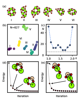
Figure 1: (a) The 6 distinct structures from which the dataset is constructed. (b) The structures from the database, plotted in two dimensions using principal component analysis. Each color represent different energy basins. (c) The result of applying the modified graph descriptor for different choices of distance cutoff $d_{k}$. The grey dashed line indicates the number of different energy basins, namely 6. (d) The energy during a local relaxation. Different colors represent different graph descriptors. The insets show a subset of atoms from the structure, where a bond between a Mg and a Si atom disappears. Bonds between atoms are shown as black lines. (e) Atoms from another structure, where a bond between two Mg atoms appears. Colors: Green - Mg, red - O, brown - Si.

To illustrate the task of classifying structures, we start by considering 6 distinct two-dimensional pyroxene (MgSiO₃)₄ compounds, as illustrated in Fig. 1(a). Each of these 6 structures are randomly perturbed three times, resulting in 18 structures in total. These 18 structures are then locally optimized in a ML energy landscape, and the trajectory from each structure relaxation is stored in a database, which results in $N=627$ configurations. The ML energy landscape is the Gaussian Process Regression model used in Sec. IV. We calculate the Fingerprint descriptorValle and Oganov (2010) of these structures and plot them in a two-dimensional space described by the first two components of a principal component analysis (PCA), which is shown in Fig. 1(b). See Sec. VIII.1 for more details about this descriptor. The colors represent which of the 6 energy basins each structure belongs to. We note that several of these structures have very similar descriptors, which stems from the fact that a lot of structures are very similar near the end of a local relaxation.

Below we introduce methods that can be used to classify structures from such a dataset. These methods are based on a simple graph representation of structures, which can be used to obtain a description of a given configuration.

II.1.1 Modified adjacency matrix classifier

We start by describing a classifier that is based on spectral graph theoryWilson and Zhu (2008); Wills and Meyer (2020). Here, a structure is described by an adjacency matrix, where the nodes correspond to the atoms, and the edges correspond to bonds between them. The adjacency matrix $A^{k}$ is defined as

$$A_{ij}^{k}=\begin{cases}0,&\text{if }i=j,\\ 1,&\text{if }d_{ij}\leq d_{k},\\ 0,&\text{otherwise},\end{cases}$$ (1)

where $d_{ij}$ is the Euclidean distance between atoms $i$ and $j$, and $d_{k}=k\cdot(r_{{\rm cov},i}+r_{{\rm cov},j})$ is a cutoff distance, where $r_{{\rm cov},i}$ is the covalent radius of atom $i$, and $k$ is a hyperparameter. By including the covalent radii of the atoms in the cutoff distance, the method is able to characterize bonds between different types of atoms. If two atoms are separated by a distance which is less than the specified cutoff distance, a value of 1 is added to the adjacency matrix, indicating that the two atoms are bound to each other.

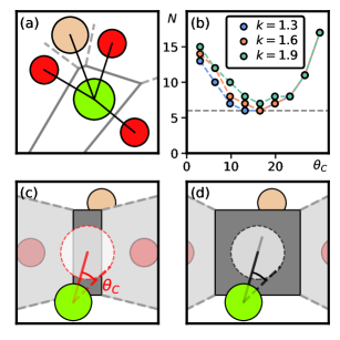
Figure 2: (a) A zoom in on a Mg atom. The grey lines indicate Voronoi faces between the atoms, and black lines indicate bonds, determined using $B^{k}$. (b) The number of unique descriptors in the database as a function of the cutoff angle $\theta_{C}$. (c) A circle centered on the possible bond between the atoms intersects with other Voronoi faces, meaning that the bond between the Mg and the Si atoms is removed. (d) A case where the circle can fit on the Voronoi face because the oxygen atoms have been moved further away from the Mg atom.

A problem with the adjacency matrix $A^{k}$ is that it does not take the atomic type of the individual atoms into account. For example, there is no way to distinguish between an A-A-B and an A-B-A configuration, where A and B are different atomic species. To solve this, we introduced a modified version of the adjacency matrix, $B^{k}$,

$$B_{ij}^{k}=\begin{cases}Z_{i},&\text{if }i=j,\\ 1,&\text{if }d_{ij}\leq d_{k},\\ 0,&\text{otherwise},\end{cases}$$ (2)

where $Z_{i}$ is the atomic number of atom $i$.

We note that the matrix $B^{k}$ is not invariant with respect to swapping indices of the atoms. Since $B^{k}$ is real and symmetric, its spectrum of eigenvalues only consists of real numbers. This can be used to define a descriptor $G$ of a structure, consisting of $N_{A}$ atoms, as

$$G=[\lambda_{1},\lambda_{2},\dots,\lambda_{N_{A}}],$$ (3)

where $\lambda_{1}\leq\lambda_{2}\leq\dots\leq\lambda_{N_{A}}$ are the $sorted$ eigenvalues of $B^{k}$. To avoid problems with numerical precisions, the eigenvalues are rounded to three decimal places. This descriptor is only based on interatomic distances, meaning that it is invariant with respect to translations and rotations of a given structure, and it is invariant with respect to the indexation of the atoms. Using this descriptor, we consider two configurations to be the same if they have identical spectra of eigenvalues, and this will be used to classify structures.

We note that for a structure containing $N_{A}$ atoms, the descriptor $G$ will contain only $N_{A}$ eigenvalues, which is less than the 3$N_{A}$-6 degrees of freedom of the system. This means that the descriptor is not guaranteed to be unique for a given structural configuration. While this is not ideal when extracting unique structures from a dataset, we have not seen any problems due to this in practice, and for the GO problems considered later on in this paper, this descriptor works well in terms of finding the GM structure.

Having designed a simple classifier, we can apply it to the dataset using different scaling parameters, $k$, for the cutoff distance. The results are shown in Fig. 1(c). It can be seen that the classifier is not able to obtain only one structure from each energy basin, and that the quality of the classifier depends heavily on the value of $k$. This can be explained by the discontinuity of the modified adjacency matrix $B^{k}$. Small changes to the position of atoms, that are separated by a distance close to the cutoff distance, can change the matrix $B^{k}$, and therefore also the descriptor $G$. This is illustrated in Fig. 1(d) and (e), where bonds between atoms appear or disappear during the local relaxation of structures. Thus, basing the classification of structures only on the distance between atoms is not a strong enough criterion if one needs to extract exactly one structure from each energy basin.

II.1.2 Voronoi tessellation

In order to get rid of the problem with atoms that are separated by a distance close to the cutoff distance, we need a more robust way of describing bonds between atoms. Looking at the structures like those in Fig. 1(d) and (e), we often observe that a major problem for the modified adjacency matrix is to determine the existence of bonds between Mg-Mg, Mg-Si, or Si-Si pairs that are separated by oxygen atoms. To tackle this problem, we want to divide space around each atom into distinct regions and quantify how much two atoms actually "see" each other.

To do this, we proceed by employing a Voronoi tessellation method together with the modified adjacency matrix. This method allows for environment aware bond criteria by considering the local environment around each atom. It works by dividing space into regions, where each region consists of all points that are closest to some prespecified points, which in this case are the positions of the atoms. The regions are separated by planes that are placed midway between atoms. These planes are referred to as Voronoi faces, and they can be used to determine if two atoms are bound to each other. In this work, we have formulated the following criteria for a bond between atoms:

1. The atoms share a Voronoi face.

2. A straight line between the two atoms passes through this Voronoi face.

3. The Voronoi face must be large enough to enclose a circle, centered on the line through the face, that spans a certain solid angle.

Figure 2(a) illustrates the Voronoi faces for a Mg atom and the atoms around it as grey lines. The Mg atom is bound to a silicon atom and three oxygen atoms, indicated by the black lines. The Mg and the Si atoms only share a small Voronoi face, which reflects that these atoms barely "see" each other, since they are screened from each other by the neighboring oxygen atoms. This is the reason for introducing the third criterion. By placing a circle on the Voronoi face, centered on the potential bond, we can control how large a Voronoi face must be in order for a bond to be valid.

The size of the circle is determined by a hyperparameter $\theta_{C}$, which we refer to as a cutoff angle. By introducing the hyperparameter $\theta_{C}$, we are now able to tune the classifier to be more or less sensitive to changes in the structure. Figures 2(c) and (d) show two examples of how the cutoff angle is used to determine whether a bond is invalid or valid, respectively. The result of this criterion, using different values of $\theta_{C}$ for three choices of $k$, is shown in Fig. 2(b). The number of structures in the dataset is greatly reduced, and the classifier is much less sensitive to the choice of scaling parameter $k$ for the cutoff distance $d_{k}$. Using this method, we are able to reduce the number of structures down to 6 for certain values of $k$ and $\theta_{C}$, meaning that we have a more reliable way of distinguishing between structures from different energy basins.

In AGOX, the Voronoi tessellation method has been implemented in a simple and computationally fast manner, where the Voronoi faces are added iteratively between atoms that are bound to each other according to the modified adjacency matrix $B^{k}$. If two atoms do not obey the three criteria above, the bond between them is removed from $B^{k}$. For computational convenience and speed, we only sample $N_{p}=8$ points on the circumference of the circle and check that they do not intersect other Voronoi faces. These points are sampled uniformly on the circle in a deterministic manner, such that the method always returns the same descriptor for a given structure.

For the atomic systems considered in this paper, the Voronoi tessellation method is the most time consuming part, compared to setting up and diagonalizing the adjacency matrix, when constructing a descriptor. However, both these tasks are much less computationally costly compared to other parts of global optimization algorithms, for example DFT calculations.

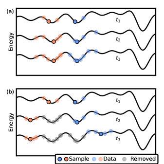
Figure 3: (a) A schematic example of a stagnated search at different times during a search. The search is stuck in a region of the PES far from the GM structure. (b) The desired effect of the filtering method. Certain structures are not allowed to enter the sample, which allows the search to focus on other parts of the PES.

II.2 Filtering of structures during global optimization search

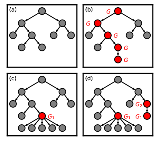
Figure 4: This figure schematically shows different situations that should be avoided during a search. The grey nodes correspond to structures, and the arrows indicate the relationship between them. In (a), no structures have been filtered out yet. The other figures show unwanted situations, namely (b) structures with the same descriptor get created over and over again, (c) the same structure produces too many new structures, (d) a structure produces a new configuration with an already removed descriptor.

Some GO algorithms rely on sampling a subset of known low-energy structures to produce new structures, which introduces the risk of stagnation, because the search keeps exploiting known regions of the PES. This is illustrated in Fig. 3(a). Here, the two sample members are always picked from the same two energy basins, and the search is prone to stagnate. To avoid this problem, a GO algorithm requires a reliable way to distinguish between structures and filter away any unwanted subset of these, which is illustrated in Fig. 3(b). To achieve this, we employ the classifier introduced in Sec. II.1. By tracking the descriptors of all structures that are found during the search, the algorithm is able to make a ’family tree’-like history of all the structures and use it to filter out unwanted structures to avoid certain scenarios to occur.

Figure 4 shows schematic examples of the history of a search and such unwanted scenarios. The grey nodes correspond to structures, and the arrows indicate which structure was modified to generate another structure, establishing a $parent$-$child$ relation between structures. In Fig. 4(a), the search is doing fine in terms of exploring different structures.

Figure 4(b) shows a situation where a chain of structures with the same descriptor $G$ has been produced. This means that the search makes new structures that are very similar to the parent structure, but which has a slightly lower energy. This situation can be seen in Fig. 3(a), where the same two local minima are being refined over and over again. This is an unwanted behavior of the sampler, since this causes the algorithm to focus too much on few parts of the PES. Therefore, we want to filter away structures with the descriptor $G$ to avoid this situation.

Figure 4(c) shows another situation where the descriptor $G_{1}$ has been used to produce five new structures. Since the same structure with description $G_{1}$ enters the sample multiple times, it means that all structures generated from it have a higher energy and will not be picked as a sample member. We therefore want to filter out structures with this specific $G_{1}$ descriptor from entering the sample, since no new structures with lower energy can be produced from them.

Finally, in Fig. 4(d), a situation is depicted where a structure with the descriptor $G_{2}$ has been used to produce a structure with the descriptor $G_{1}$. This indicates that the structure with descriptor $G_{2}$ is close to the structures with descriptor $G_{1}$ in the configurational space, meaning that the search is still focusing on a region of the PES that has already been exploited. Since we have removed structures with the descriptor $G_{1}$, we also want to filter out structures with the descriptor $G_{2}$.

To avoid these unwanted situations from Fig. 4 to occur, we require that structures with a descriptor $G$ do not produce more than $N_{\rm max}$ new structures, and that they do not produce new structures with already removed descriptors. By doing so, we allow the algorithm to leave a region of the PES that it has exploited, and focus on new, unknown regions, which is illustrated in Fig. 3(b). This filtering method will be referred to as the Family Tree Filtering (FTF) method.

III The GOFEE algorithm

Now that we have identified scenarios we want to avoid during a search, we can test the FTF method in a GO algorithm. In this work, we focus on the Global Optimization with First-principles Energy Expressions (GOFEE) algorithm. GOFEE is an iterative search method that combines elements from EAs with ML methods. In each iteration, a subset of previously found structures are sampled. These sampled structures, also referred to as $parents$, are modified to create $N_{C}$ new structures. The new structures are locally optimized in an uncertainty-aware machine learned energy model, and the structure with lowest confidence bound (= predicted energy minus some degree of predicted uncertainty), according to this ML model, is evaluated in the target potential, i.e., DFT or LJ. More details about the GOFEE algorithm can be found in the Appendix, Sec. VIII.2.

The sampling of known structures to obtain the parent structures is based on the k-means algorithm. This sampling method was introduced in Ref. Merte et al., 2022, where it was shown to increase the performance of the GOFEE algorithm. In this method, all evaluated structures with an energy $E>E_{\rm min}+5\ \rm eV$ are removed from the pool of potential sample structures, where $E_{\rm min}$ is the lowest energy found so far. The remaining structures are clustered into $N_{k}$ clusters, where $N_{k}$ is a predefined hyperparameter equal to the desired number of sampled structures. Finally, the sample of parent structures is constructed by extracting the lowest energy structure from each of the $N_{k}$ clusters. A schematic one-dimensional example of this is shown in Fig. 3(a) with $N_{k}=2$ and at different times of the search. When the FTF method is employed in GOFEE, it will be used to filter out unwanted structures before the k-means sampling takes place, such that the sample keeps evolving during the search as illustrated in Fig. 3(b).

We resort to success curves to compare the performance of the GOFEE algorithm with and without the FTF method. To construct a success curve, a GOFEE search is started 100 times with the same settings but different initial atomistic configurations. For each of these 100 searches, the initial configurations were constructed by randomly placing the atoms in a large confinement cellChristiansen, Rønne, and Hammer (2022). The success curve $s(x)$ then measures the proportion of these individual searches that have found a structure with the same descriptor as the GM structure after $x$ number of single-point calculations. We will compare success curves from different searches that either uses the FTF method or not. Not using the FTF method corresponds to setting $N_{\rm max}=\infty$, which we will use as the notation for such searches.

IV Application to a 2-dimensional test system

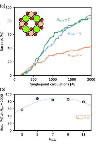
Figure 5: (a) The success curves of the GOFEE algorithm with the FTF method when searching for the GM structure of the 2-dimensional pyroxene system. (b) The final success after 2000 target evaluations for different choices of $N_{\rm max}$. The grey line is plotted to guide the eye.

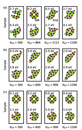
Figure 6: The evolution of the sample of (a) a successful search using $N_{\rm max}=5$, (b) an unsuccessful and (c) a successful GOFEE search with $N_{\rm max}=\infty$ after $N_{SP}$ number of target evaluations. The number above each structure indicates its energy relative to that of the GM structure. The GM configuration from (a) was not fully optimized before the FTF method filtered it away, meaning that a relaxation of the remaining energy of 0.2 eV was not obtained.

This section shows the results of introducing the FTF method when searching for the GM structure of the 2-dimensional pyroxene (MgSiO₃)₄ system. The target potential was a pretrained Gaussian Process RegressionRasmussen and Williams (2005) (GPR) model, trained on 314 pyroxene structures. A small sample size $N_{k}=2$ was used in order to visualize the evolution of the sample during searches. The success curves with and without the filtering can be seen in Fig. 5(a). The figure shows that employing the FTF method increased the performance of GOFEE in terms of finding the GM structure.

Figure 5(b) shows the final success after 2000 target evaluations for different choices of $N_{\rm max}$. It can be seen that the performance of GOFEE using the FTF method greatly depends on the choice of $N_{\rm max}$. If $N_{\rm max}$ is too low, e.g. 3, the final success is lower compared to larger values of $N_{\rm max}$, but it is still better than not using the filtering at all. This shows that filtering is indeed useful for the GOFEE algorithm.

The evolution of the sample from different searches can be compared to investigate the behavior of the sample members. In Fig. 6(a), the evolution of the sample in one of the successful GOFEE searches, which used the FTF method, is shown. The GM structure was found after 884 target evaluation, while the second best configuration was found after 1112 target evaluations. This demonstrates that the search is indeed capable of exploring various regions of the PES during a single search when employing the FTF method, which is the desired outcome of adding the method to the GOFEE algorithm.

This can be compared to samples from GOFEE searches that did not employ the FTF method. Figure 6(b) shows the evolution of the sample of an unsuccessful GOFEE search. Clearly, up to iteration 900, the sample consisted of progressively lower energy structures, but from then on the sample did not evolve, meaning that the search was stuck in some region of the PES. Fig. 6(c) shows the sample from a successful GOFEE search. The GM structure was obtained in less than 300 iterations, but the sample did not change at all during the remaining part of the search, except for some energy reduction of the already found structures. Even though this search was successful, it does not find the second best structure, shown in Fig. 6(a), indicating that the search could not escape these low-energy regions of the PES.

V Further applications

Now that we have demonstrated the effect of adding the filtering method to GOFEE, we will apply it to solve more interesting problems. In this section, GOFEE will be used to find the GM structure of a 3-dimensional olivine compound and a Au₁₂ configuration. The target potential will be DFT using the Perdew-Becke-Ernzerhof (PBE)Perdew, Burke, and Ernzerhof (1996) exchange-correlation functional and a LCAOLarsen et al. (2009) basis using the GPAWEnkovaara et al. (2010) module. In both cases, the structures were placed in a $20\times 20\times 20$ ų box. A sample size of $N_{k}=5$ was used in both cases. To further show the usefulness of the FTF method in the GOFEE algorithm, we employ the computationally cheap Lennard-Jones potential to search for larger compunds. The GOFEE algorithm is used to find the GM structure of the LJ₅₅ systems. After that, we turn off the ML part of GOFEE in order to solve an even larger problem, namely the LJ₇₅ system.

V.1 Olivine compound

In this section, GOFEE was used to solve the problem of finding the GM structure of a 3-dimensional olivine (Mg₂SiO₄)₄ compoundSlavensky, Christiansen, and Hammer (2023). Nanosized silicate compounds are found to be abundant in the Interstellar MediumLi and Draine (2001), and several properties of these systems have been computationally studiedTang, Bromley, and Hammer (2023); Escatllar et al. (2019); Goumans and Bromley (2011); Mariñoso Guiu et al. (2021); Woodley (2009); Zeegers et al. (2023).

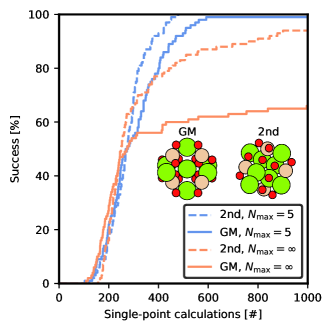
Figure 7: The success curves for finding both the GM structure and the second lowest energy structure during searches of the 3-dimensional olivine (Mg₂SiO₄)₄ system. For both structures, using the filtering method before sampling improved the performance of finding both of them.

Figure 7 shows the success curves for finding both the GM structure and the second-lowest energy structure. By using the filtering method before the sampling, nearly all searches were able to find both the GM and the second-lowest energy structure during the same search. It is clear that some of the searches, which did not employ the filtering method, could also find the GM, but in 1/3 of the searches the GM was not found at all. On the other hand, it seems that almost all of them eventually find the second best structure, but it happened much later compared to the searches that used the filtering process. This could indicate that these searches spent too many resources exploring regions of the PES that were not relevant for finding the GM structure.

V.2 Small gold configuration

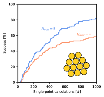
Figure 8: Succes curves for finding the GM of Au₁₂, shown in the inset, using the GOFEE algorithm with and without the FTF method.

GOFEE was used to solve the global optimization problem of finding the global energy minimum structure of the Au₁₂ cluster. Small gold systems have previously been investigatedFa, Luo, and Dong (2005); Xing et al. (2006); Chaves, Piotrowski, and Da Silva (2017). It has been shown that the GM structure of the smaller gold clusters tend to be planar, while low-energy three-dimensional configurations exist at the same time. On the other hand, the GM configurations of the larger compounds often appear to be three-dimensional. This fact potentially increases the complexity of the problem, since the GOFEE algorithm might get stuck searching for 3-dimensional configurations while the GM actually is planar, and vice versa.

The planar GM structure for this global optimization problem is shown in the inset in Fig. 8. We allow the search to be fully three-dimensional in order to increase the difficulty of the problem. Fig. 8 evidences that the filtering method improves the performance of the GOFEE algorithm.

V.3 LJ₅₅

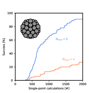
Figure 9: The succes curves for finding the GM of the LJ₅₅ system with and without the FTF method.

To further examine the performance of the FTF method, we wanted to test it on a larger system. To do this we used the Lennard-Jones potential, since the energy evaluations are fast to perform compared to DFT, and because the GM structures of various LJ systems are well-knownWales and Doye (1997). We therefore applied the method to the LJ₅₅ system. This system has three highly symmetric minima, making it a potentially difficult problem to solve.

The success curves for different searches can be seen in Fig. 9. The figure demonstrates that the GOFEE algorithm greatly benefits from using the filtering method, since the problem can be solved almost every time within 2000 single-point evaluations.

V.4 LJ₇₅

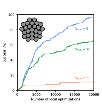
Figure 10: Different succes curves when using a modified GOFEE algorithm with and without the FTF method to find the GM of the LJ₇₅ structure.

We now turn our attention to the LJ₇₅ systemWales and Doye (1997). For a system of this size, the configurational space is much larger compared to the LJ₅₅ system, meaning that a large number of energy evaluations are required to solve the problem. At the same time, such evaluations using the Lennard-Jones formula are quite fast, meaning that the machine learning part of GOFEE quickly becomes the time-dominating factor. To combat this problem, we modified the GOFEE algorithm such that no ML is used during the search. All structures are locally optimized directly in the LJ potential instead, making it possible to perform longer global optimization searches. More details about the modified GOFEE algorithm can be found in the Appendix, sec. VIII.3.

The succes curves for solving this problem can be seen in Fig. 10. Without the FTF method, the problem is really difficult to solve for the modified GOFEE algorithm, indicating that the search potentially becomes stuck in unwanted regions of the PES. Using the FTF method greatly improves the chance of finding the GM configuration, demonstrating that the method increases the performance of the GO algorithm.

VI Conclusion

We have proposed a method for classifying structures from different energy basins in a dataset. This method employed spectral graph theory and the Voronoi tessellation method to make it robust to small variations to the structures, and we have shown its capability of distinguishing structures from different energy minima. The classifier was introduced to the GOFEE algorithm as a filtering mechanism for the sampling of known structures. By doing so, the algorithm was able to abandon regions of the PES that it had exploited and thereby avoid stagnation. We have shown that the filtering method greatly improves the performance of the GOFEE algorithm when searching for an olivine (Mg₂SiO₄)₄, a Au₁₂, and a LJ₅₅ system, and that a modified GOFEE algorithm benefits from using the filtering method when solving the LJ₇₅ system.

VII Acknowledgements

This work has been supported by VILLUM FONDEN through Investigator grant, project no. 16562, and by the Danish National Research Foundation through the Center of Excellence “InterCat” (Grant agreement no: DNRF150).

Data availability

The data that support the findings of this study and the corresponding AGOX scripts are available at https://gitlab.com/aslavensky/classifier_paper. The AGOX code can be obtained from https://gitlab.com/agox/agox. The documentation for the AGOX module can be found at https://agox.gitlab.io/agox.

References

VIII Appendix

VIII.1 Fingerprint descriptor

To train a machine learning model, a translational and rotational invariant descriptor of atomic systems is required. In GOFEE, the Fingerprint descriptorValle and Oganov (2010) by Valle and Oganov is used. Here, the radial part of the descriptor is evaluated as

$$F_{AB}(r) \propto\begin{cases}\sum_{i,j}\frac{1}{r_{ij}^{2}}\text{exp}\left(-\frac{(r-r_{ij})^{2}}{2l_{r}^{2}}\right)&,\quad r<R_{r}\\ 0&,\quad r\geq R_{r}\end{cases}$$

and the angular part is calculated as

$$F_{ABC}(\theta) \propto\sum_{i,j,k}f_{c}(r_{ij})f_{c}(r_{ik})\text{exp}\left(-\frac{(\theta-\theta_{ikj})^{2}}{2l_{\theta}^{2}}\right),$$

where $A$, $B$, and $C$ are atomic types, $R_{r}=6$ Å is a radial cutoff distance, $l_{r}=0.2$ Å, $l_{\theta}=0.2$ rad, and $f_{c}$ is a cutoff function. For a given structure, all two-body (radial) and three-body (angular) combinations of the atomic types are calculated and binned into 30 bins. These bins are concatenated into a single feature vector that describes the whole atomistic system.

VIII.2 The GOFEE algorithm

In this work, we focus on the GOFEE algorithmBisbo and Hammer (2020, 2022). GOFEE combines elements from EAs and machine learning (ML) to reduce the required number of target potential evaluations required to find the GM structure. To avoid spending a lot of computational resources on doing local optimizations of new structures in the target potential, which could become time-consuming when using DFT, GOFEE employs a ML surrogate model for the structure relaxation. The surrogate model, which is trained on-the-fly, is constructed using Gaussian Process Regression (GPR)Rasmussen and Williams (2005). Given a database of training data X, which is a matrix consisting of the Fingerprint representationsValle and Oganov (2010) of the structures, and a vector of their corresponding energies E, the GPR model can predict the energy of a new structure $\textbf{x}_{*}$, $E_{GPR}(\textbf{x}_{*})$, and the model’s uncertainty of the predicted energy, $\sigma_{GPR}(\textbf{x}_{*})$, as

$$E_{GPR}(\textbf{x}_{*}) =K(\textbf{x}_{*},\textbf{X})\textbf{C}(\textbf{E}-\bm{\mu})+\mu(\textbf{x}_{*}),$$ (VIII.21)

$$\sigma_{GPR}(\textbf{x}_{*}) =K(\textbf{x}_{*},\textbf{x}_{*})-K(\textbf{x}_{*},\textbf{X})\textbf{C}K(\textbf{X},\textbf{x}_{*}),$$ (VIII.22)

where $\bm{\mu}$ is a vector containing the prior values of each training structure, $K$ is the kernel function, and $\textbf{C}=[K(\textbf{X},\textbf{X})+\sigma_{n}^{2}\textbf{I}]^{-1}$, where $\sigma_{n}=10^{-2}$ eV acts as regularization. In GOFEE, the kernel $K$ is given as

$$K(\textbf{x}_{i},\textbf{x}_{j})= \theta_{0}(1-\beta)\text{exp}\left(-\frac{1}{2}\left[\frac{\textbf{x}_{i}-\textbf{x}_{j}}{\lambda_{1}}\right]^{2}\right)+$$

$$\theta_{0}\beta\text{exp}\left(-\frac{1}{2}\left[\frac{\textbf{x}_{i}-\textbf{x}_{j}}{\lambda_{2}}\right]^{2}\right)$$ (VIII.23)

where $\beta=0.01$ is the weight between the two Gaussians, $\theta_{0}$ is the amplitude of the kernel, and $\lambda_{1}>\lambda_{2}$ are length scales. The prior $\mu$ is given by

$$\mu(\textbf{x})=\bar{E}+\frac{1}{2}\sum_{ab}\left(\frac{1\text{\r{A}}}{r_{ab}+1\text{\r{A}}-0.7r_{CD,ab}}\right)^{12}\text{eV},$$ (VIII.24)

where $r_{ab}$ is the distance between atoms $a$ and $b$, $r_{CD,ab}$ is the sum of their covalent radii, and $\bar{E}$ is the mean energy of the training data.

Using these quantities, a lower confidence bound (LCB) energy expressions can be formulated,

$$E_{\rm LCB}(\textbf{x}_{*})=E_{GPR}(\textbf{x}_{*})-\kappa\sigma_{GPR}(\textbf{x}_{*}),$$ (VIII.25)

where $\kappa=2$ is a hyperparameter that controls the trade-off between exploration and exploitation of the PES. This energy model is used in GOFEE to do local optimization of structures. More details about the GPR model can be found in Ref. Bisbo and Hammer, 2022.

The GOFEE algorithm starts out by making completely random structures, evaluating their energies, adding them to a database, and construct the initial surrogate model. From then on, it iteratively samples the database, makes new structures, and improves the surrogate model in its attempt of finding the GM structure. GOFEE can be summarized as follows:

1. Sample $N_{k}$ parent structures from the database of previously evaluated structures.

2. Modify these parent structures to obtain $N_{C}$ new structures.

3. Locally optimize all $N_{C}$ new structures in the LCB landscape.

4. Pick the structure with the lowest energy predicted by the LCB energy expression.

5. Evaluate its energy in the target potential.

6. Add the new structure and its energy to the database. Retrain the surrogate model.

7. Repeat steps 1-6 until a certain number of iterations has been done.

VIII.3 Modified GOFEE algorithm

The difference between the GOFEE algorithm and the modified version of it, used to solve the LJ₇₅ system, is that the modified GOFEE algorithm does not employ ML. This choice was made to investigate the performance of the FTF method for a large well-known problem. The modified GOFEE algorithm can be summarized as follows:

1. Sample $N_{k}$ parent structures from the database of previously evaluated structures.

2. Modify these parent structures to obtain $N_{C}$ new structures.

3. Optimize all $N_{C}$ structures in the LJ potential and add them to the database.

4. Repeat steps 1-3 until a certain number of iterations has been done.

References

- Huang et al. (2017) S.-D. Huang, C. Shang, X.-J. Zhang, and Z.-P. Liu, Chem. Sci. 8, 6327 (2017).
- Deringer et al. (2018) V. L. Deringer, D. M. Proserpio, G. Csányi, and C. J. Pickard, Faraday Discussions 211, 45 (2018).
- Paleico and Behler (2020) M. L. Paleico and J. Behler, The Journal of Chemical Physics 153, 054704 (2020).
- Arrigoni and Madsen (2021) M. Arrigoni and G. K. H. Madsen, npj Computational Materials 7, 1 (2021).
- Kaappa, Larsen, and Jacobsen (2021) S. Kaappa, C. Larsen, and K. W. Jacobsen, Physical Review Letters 127, 166001 (2021).
- Han et al. (2022) S. Han, G. Barcaro, A. Fortunelli, S. Lysgaard, T. Vegge, and H. A. Hansen, npj Comput. Mater. 8, 121 (2022).
- Pierre Lourenço et al. (2022) M. Pierre Lourenço, L. Barrios Herrera, J. Hostaš, P. Calaminici, A. M. Köster, A. Tchagang, and D. R. Salahub, Physical Chemistry Chemical Physics 24, 25227 (2022).
- Jung et al. (2022) H. Jung, L. Sauerland, S. Stocker, K. Reuter, and J. T. Margraf, “Machine-Learning Driven Global Optimization of Surface Adsorbate Geometries,” (2022).
- Merte et al. (2022) L. R. Merte, M. K. Bisbo, I. Sokolović, M. Setvín, B. Hagman, M. Shipilin, M. Schmid, U. Diebold, E. Lundgren, and B. Hammer, Angewandte Chemie International Edition 61, e202204244 (2022).
- Chen, Shang, and Liu (0022) D. Chen, C. Shang, and Z.-P. Liu, J. Chem. Phys. 156, 094104 (20022).
- Rønne et al. (2022) N. Rønne, M.-P. V. Christiansen, A. M. Slavensky, Z. Tang, F. Brix, M. E. Pedersen, M. K. Bisbo, and B. Hammer, The Journal of Chemical Physics 157, 174115 (2022).
- Larsen et al. (2023) C. Larsen, S. Kaappa, A. L. Vishart, T. Bligaard, and K. W. Jacobsen, Physical Review B 107, 214101 (2023).
- Shi et al. (2023) X. Shi, D. Cheng, R. Zhao, G. Zhang, S. Wu, S. Zhen, Z.-J. Zhao, and J. Gong, Chem. Sci. 14, 8777 (2023).
- Kim et al. (2024) H. J. Kim, G. Lee, S.-H. V. Oh, C. Stampfl, and A. Soon, ACS Nano 18, 4559–4569 (2024).
- Li, Kermode, and De Vita (2015) Z. Li, J. R. Kermode, and A. De Vita, Physical Review Letters 114, 096405 (2015).
- Deringer and Csányi (2017) V. L. Deringer and G. Csányi, Physical Review B 95, 094203 (2017).
- Jindal, Chiriki, and Bulusu (2017) S. Jindal, S. Chiriki, and S. S. Bulusu, The Journal of Chemical Physics 146, 204301 (2017).
- Roongcharoen et al. (2023) T. Roongcharoen, X. Yang, S. Han, L. Sementa, T. Vegge, H. Anton Hansen, and A. Fortunelli, Faraday Discuss. 242, 174 (2023).
- Xie et al. (2023) Y. Xie, J. Vandermause, S. Ramakers, N. H. Protik, A. Johansson, and B. Kozinsky, npj Computational Materials 9, 36 (2023).
- Jinnouchi et al. (2019) R. Jinnouchi, J. Lahnsteiner, F. Karsai, G. Kresse, and M. Bokdam, Physical Review Letters 122, 225701 (2019).
- Rosenbrock et al. (2021) C. W. Rosenbrock, K. Gubaev, A. V. Shapeev, L. B. Pártay, N. Bernstein, G. Csányi, and G. L. W. Hart, npj Computational Materials 7, 24 (2021).
- Rossignol et al. (2024) H. Rossignol, M. Minotakis, M. Cobelli, and S. Sanvito, Journal of Chemical Information and Modeling 64, 1828 (2024).
- Gastegger, Behler, and Marquetand (2017) M. Gastegger, J. Behler, and P. Marquetand, Chemical Science 8, 6924 (2017).
- Beckmann et al. (2022) R. Beckmann, F. Brieuc, C. Schran, and D. Marx, Journal of Chemical Theory and Computation 18, 5492 (2022).
- Tang, Bromley, and Hammer (2023) Z. Tang, S. T. Bromley, and B. Hammer, The Journal of Chemical Physics 158, 224108 (2023).
- Ouyang, Xie, and Jiang (2015) R. Ouyang, Y. Xie, and D.-e. Jiang, Nanoscale 7, 14817 (2015).
- Smith et al. (2018) J. S. Smith, B. Nebgen, N. Lubbers, O. Isayev, and A. E. Roitberg, The Journal of Chemical Physics 148, 241733 (2018).
- Sivaraman et al. (2020) G. Sivaraman, A. N. Krishnamoorthy, M. Baur, C. Holm, M. Stan, G. Csányi, C. Benmore, and A. Vazquez-Mayagoitia, npj Computational Materials 6, 104 (2020).
- Vandermause et al. (2020) J. Vandermause, S. B. Torrisi, S. Batzner, Y. Xie, L. Sun, A. M. Kolpak, and B. Kozinsky, npj Comput. Mater. 6, 20 (2020).
- Timmermann et al. (2021) J. Timmermann, Y. Lee, C. G. Staacke, J. T. Margraf, C. Scheurer, and K. Reuter, The Journal of Chemical Physics 155, 244107 (2021).
- Yang, Jiménez-Negrón, and Kitchin (2021) Y. Yang, O. A. Jiménez-Negrón, and J. R. Kitchin, The Journal of Chemical Physics 154, 234704 (2021).
- Van Der Oord et al. (2023) C. Van Der Oord, M. Sachs, D. P. Kovács, C. Ortner, and G. Csányi, npj Computational Materials 9, 168 (2023).
- Wang et al. (2023) J. Wang, H. Gao, Y. Han, C. Ding, S. Pan, Y. Wang, Q. Jia, H.-T. Wang, D. Xing, and J. Sun, National Science Review 10, nwad128 (2023).
- Irwin and Shoichet (2005) J. J. Irwin and B. K. Shoichet, Journal of Chemical Information and Modeling 45, 177 (2005).
- Ruddigkeit et al. (2012) L. Ruddigkeit, R. van Deursen, L. C. Blum, and J.-L. Reymond, Journal of Chemical Information and Modeling 52, 2864 (2012).
- Jain et al. (2013) A. Jain, S. P. Ong, G. Hautier, W. Chen, W. D. Richards, S. Dacek, S. Cholia, D. Gunter, D. Skinner, G. Ceder, and K. A. Persson, APL Materials 1, 011002 (2013).
- Winther et al. (2019) K. T. Winther, M. J. Hoffmann, J. R. Boes, O. Mamun, M. Bajdich, and T. Bligaard, Scientific Data 6, 75 (2019).
- Schreiner et al. (2022) M. Schreiner, A. Bhowmik, T. Vegge, J. Busk, and O. Winther, Scientific Data 9, 779 (2022).
- Andersen and Slavensky (2023) M. Andersen and A. M. Slavensky, The Journal of Chemical Physics 159, 044711 (2023).
- Valle and Oganov (2010) M. Valle and A. R. Oganov, Acta Crystallographica. Section A, Foundations of Crystallography 66, 507 (2010).
- Schütt et al. (2014) K. T. Schütt, H. Glawe, F. Brockherde, A. Sanna, K. R. Müller, and E. K. U. Gross, Physical Review B 89, 205118 (2014).
- Hansen et al. (2015) K. Hansen, F. Biegler, R. Ramakrishnan, W. Pronobis, O. A. von Lilienfeld, K.-R. Müller, and A. Tkatchenko, The Journal of Physical Chemistry Letters 6, 2326 (2015).
- Behler (2011) J. Behler, The Journal of Chemical Physics 134, 074106 (2011).
- Bartók, Kondor, and Csányi (2013) A. P. Bartók, R. Kondor, and G. Csányi, Physical Review B 87, 184115 (2013).
- Drautz (2019) R. Drautz, Physical Review B 99, 014104 (2019).
- Rupp et al. (2012) M. Rupp, A. Tkatchenko, K.-R. Müller, and O. A. von Lilienfeld, Physical Review Letters 108, 058301 (2012).
- Faber et al. (2015) F. Faber, A. Lindmaa, O. A. von Lilienfeld, and R. Armiento, International Journal of Quantum Chemistry 115, 1094 (2015).
- Zhu et al. (2016) L. Zhu, M. Amsler, T. Fuhrer, B. Schaefer, S. Faraji, S. Rostami, S. A. Ghasemi, A. Sadeghi, M. Grauzinyte, C. Wolverton, and S. Goedecker, The Journal of Chemical Physics 144, 034203 (2016).
- Schütt et al. (2018) K. T. Schütt, H. E. Sauceda, P.-J. Kindermans, A. Tkatchenko, and K.-R. Müller, The Journal of Chemical Physics 148, 241722 (2018).
- (50) K. Schütt, O. Unke, and M. Gastegger, Proceedings of the 38th International Conference on Machine Learning, (PMLR, 2021) , p. 9377.
- Batzner et al. (2022) S. Batzner, A. Musaelian, L. Sun, M. Geiger, J. P. Mailoa, M. Kornbluth, N. Molinari, T. E. Smidt, and B. Kozinsky, Nature Communications 13, 2453 (2022).
- Batatia et al. (2022) I. Batatia, D. P. Kovacs, G. Simm, C. Ortner, and G. Csanyi, Advances in Neural Information Processing Systems 35, 11423 (2022).
- Xu, Reuter, and Andersen (2022) W. Xu, K. Reuter, and M. Andersen, Nat Comput Sci 2, 443450 (2022).
- Deng et al. (2023) B. Deng, P. Zhong, K. Jun, J. Riebesell, K. Han, C. J. Bartel, and G. Ceder, Nature Machine Intelligence 5, 1031 (2023).
- Bartók et al. (2017) A. P. Bartók, S. De, C. Poelking, N. Bernstein, J. R. Kermode, G. Csányi, and M. Ceriotti, Science Advances 3, e1701816 (2017).
- Tahmasbi, Goedecker, and Ghasemi (2021) H. Tahmasbi, S. Goedecker, and S. A. Ghasemi, Physical Review Materials 5, 083806 (2021).
- Lee et al. (2023) Y. Lee, J. Timmermann, C. Panosetti, C. Scheurer, and K. Reuter, The Journal of Physical Chemistry C 127, 17599 (2023).
- Hartke (1995) B. Hartke, Chemical Physics Letters 240, 560 (1995).
- Johnston (2003) R. L. Johnston, Dalton Transactions 22, 4193 (2003).
- Vilhelmsen and Hammer (2014) L. B. Vilhelmsen and B. Hammer, The Journal of Chemical Physics 141, 044711 (2014).
- Hartke (1999) B. Hartke, Journal of Computational Chemistry 20, 1752 (1999).
- Goedecker (2004) S. Goedecker, The Journal of Chemical Physics 120, 9911 (2004).
- Krummenacher et al. (2024) M. Krummenacher, M. Gubler, J. A. Finkler, H. Huber, M. Sommer-Jörgensen, and S. Goedecker, SoftwareX 25, 101632 (2024).
- Wilson and Zhu (2008) R. C. Wilson and P. Zhu, Pattern Recognition 41, 2833 (2008).
- Wills and Meyer (2020) P. Wills and F. G. Meyer, PLOS ONE 15, e0228728 (2020).
- O’Keeffe (1979) M. O’Keeffe, Acta Crystallographica Section A 35, 772 (1979).
- Pan et al. (2021) H. Pan, A. M. Ganose, M. Horton, M. Aykol, K. A. Persson, N. E. R. Zimmermann, and A. Jain, Inorganic Chemistry 60, 1590 (2021).
- Ward et al. (2017) L. Ward, R. Liu, A. Krishna, V. I. Hegde, A. Agrawal, A. Choudhary, and C. Wolverton, Physical Review B 96, 024104 (2017).
- Park and Wolverton (2020) C. W. Park and C. Wolverton, Physical Review Materials 4, 063801 (2020).
- Bisbo and Hammer (2020) M. K. Bisbo and B. Hammer, Physical Review Letters 124, 086102 (2020).
- Bisbo and Hammer (2022) M. K. Bisbo and B. Hammer, Physical Review B 105, 245404 (2022).
- Christiansen, Rønne, and Hammer (2022) M.-P. V. Christiansen, N. Rønne, and B. Hammer, The Journal of Chemical Physics 157, 054701 (2022).
- Rasmussen and Williams (2005) C. E. Rasmussen and C. K. I. Williams, Gaussian Processes for Machine Learning (The MIT Press, 2005).
- Perdew, Burke, and Ernzerhof (1996) J. P. Perdew, K. Burke, and M. Ernzerhof, Physical Review Letters 77, 3865 (1996).
- Larsen et al. (2009) A. H. Larsen, M. Vanin, J. J. Mortensen, K. S. Thygesen, and K. W. Jacobsen, Physical Review B 80, 195112 (2009).
- Enkovaara et al. (2010) J. Enkovaara, C. Rostgaard, J. J. Mortensen, J. Chen, M. Dułak, L. Ferrighi, J. Gavnholt, C. Glinsvad, V. Haikola, H. A. Hansen, H. H. Kristoffersen, M. Kuisma, A. H. Larsen, L. Lehtovaara, M. Ljungberg, O. Lopez-Acevedo, P. G. Moses, J. Ojanen, T. Olsen, V. Petzold, N. A. Romero, J. Stausholm-Møller, M. Strange, G. A. Tritsaris, M. Vanin, M. Walter, B. Hammer, H. Häkkinen, G. K. H. Madsen, R. M. Nieminen, J. K. Nørskov, M. Puska, T. T. Rantala, J. Schiøtz, K. S. Thygesen, and K. W. Jacobsen, Journal of Physics: Condensed Matter 22, 253202 (2010).
- Slavensky, Christiansen, and Hammer (2023) A. M. Slavensky, M.-P. V. Christiansen, and B. Hammer, The Journal of Chemical Physics 159, 024123 (2023).
- Li and Draine (2001) A. Li and B. T. Draine, The Astrophysical Journal 550, L213 (2001).
- Escatllar et al. (2019) A. M. Escatllar, T. Lazaukas, S. M. Woodley, and S. T. Bromley, ACS Earth and Space Chemistry 3, 2390 (2019).
- Goumans and Bromley (2011) T. P. M. Goumans and S. T. Bromley, Monthly Notices of the Royal Astronomical Society 414, 1285 (2011).
- Mariñoso Guiu et al. (2021) J. Mariñoso Guiu, S. Ferrero, A. Macià Escatllar, A. Rimola, and S. T. Bromley, Frontiers in Astronomy and Space Sciences 8, 676548 (2021).
- Woodley (2009) S. Woodley, Materials and Manufacturing Processes 24, 255 (2009).
- Zeegers et al. (2023) S. T. Zeegers, J. M. Guiu, F. Kemper, J. P. Marshall, and S. T. Bromley, Faraday Discussions 245, 609 (2023).
- Fa, Luo, and Dong (2005) W. Fa, C. Luo, and J. Dong, Physical Review B 72, 205428 (2005).
- Xing et al. (2006) X. Xing, B. Yoon, U. Landman, and J. H. Parks, Physical Review B 74, 165423 (2006).
- Chaves, Piotrowski, and Da Silva (2017) A. S. Chaves, M. J. Piotrowski, and J. L. F. Da Silva, Physical Chemistry Chemical Physics 19, 15484 (2017).
- Wales and Doye (1997) D. J. Wales and J. P. K. Doye, The Journal of Physical Chemistry A 101, 5111 (1997).