\ul
\authorinfoFurther author information: (Send correspondence to S.M.)
S.M: E-mail: siddharth@saao.ac.za, sidh345@gmail.com
Improving polarimetric accuracy of RoboPol to 0.05 % using a half-wave plate calibrator system
Abstract
RoboPol is a four-channel, one-shot linear optical polarimeter that has been successfully operating since 2013 on the 1.3 m telescope at Skinakas Observatory in Crete, Greece. Using its unique optical system, it measures the linear Stokes parameters and in a single exposure with high polarimetric accuracy of 0.1%-0.15% and 1 degree in polarization angle in the R broadband filter. Its performance marginally degrades in other broadband filters.
The source of the current instrumental performance limit has been identified as unaccounted and variable instrumental polarization, most likely originating from factors such as temperature and gravity-induced instrument flexure. To improve the performance of RoboPol in all broadband filters, including R, we have developed a rotating half-wave plate calibrator system. This calibrator system is placed at the beginning of the instrument and enables modulation of polarimetric measurements by beam swapping between all four channels of RoboPol.
Using the new calibrator system, we observed multiple polarimetric standard stars over two annual observing seasons with RoboPol. This has enabled us to achieve a polarimetric accuracy of better than 0.05 % in both and , and 0.5 degrees in polarization angle across all filters, enhancing the instrument’s performance by a factor of two to three.
keywords:
optical polarimeter, polarimetry, polarization, linear polarimetry, imaging polarimetry, RoboPol, one-shot polarimetry, polarimetric calibration1 INTRODUCTION
The Robotic Polarimeter (RoboPol) is a four-channel, one-shot optical linear polarimeter mounted on the 1.3 m telescope at Skinakas Observatory in Crete, Greece[1, 2]. It was commissioned in 2013 and has been working successfully since. It is operated by the Institute of Astrophysics, Foundation for Research and Technology-Hellas (FORTH) in Crete, Greece. Since its commissioning, it has been a heavily used instrument. Data obtained by RoboPol have enabled research output in the form of publications in various fields of astronomy, including blazars[3], gamma-ray bursts[4], and interstellar medium physics[5, 6, 7]. A comprehensive list of publications resulting from RoboPol data can be found on the RoboPol program’s webpage111https://robopol.physics.uoc.gr/publications.
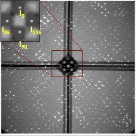
RoboPol’s polarization analyzer system consists of two quartz Wollaston Prisms (WPs), each with its own half-wave plate (HWP) at the front. The two WPs share a collimated beam created by upstream collimator optics. Four beams polarized along the , , and axes are split from this input beam and imaged as four spots in close proximity on the CCD detector, as shown in Figure 1. Linear Stokes parameters and are obtained by performing relative photometry on the four images.
RoboPol is mounted on the direct Cassegrain focus of the telescope. While it has a large field of view of , its performance is optimized inside the central region of , which is masked from neighboring regions to reduce the sky background. For a detailed description of the instrument design, we refer readers to the RoboPol instrument design and commissioning paper by Ramaprakash et al.[1]. The instrument was planned and designed for long-term high-accuracy and efficient monitoring of point sources such as blazars. Using measurements of on-sky polarized and unpolarized standard stars, the accuracy of RoboPol in degree of linear polarization, , has been found to be between 0.1% and 0.2% in the R-band and marginally worse in other bands.
Besides its primary role in executing the core RoboPol scientific program, the RoboPol instrument also serves as a test-bed for the forthcoming PASIPHAE sky survey. This survey will utilize RoboPol’s successor, the Wide-Area Linear Optical Polarimeter (WALOP) instruments. In preparation for the PASIPHAE program, RoboPol was instrumental in conducting two key projects: (a) a five-year monitoring initiative, which led to the creation of an extensive catalog of optical polarimetric standard stars[8], and (b) the identification of new wide-field sources for calibrating wide-field instruments[9, 10].
In terms of instrument calibration and characterization, RoboPol is employed to test calibration methods for WALOP polarimeters. This paper focuses on one specific idea: enhancing the calibration and accuracy of four-channel one-shot polarimeters, such as RoboPol and WALOP, by utilizing a modulating HWP in conjugation with their one-shot polarimetry capacity.
To first order, and with accuracy sufficient for RoboPol, the relation of measured Stokes parameters and to the true Stokes parameters of a source and can be written in the form of Equations 1 and 2. Please refer to Appendix A for derivation of these equations and their relation to the instrument Mueller matrix. In general, these values can depend on all the intrinsic Stokes parameters of the source. The and terms are the polarimetric efficiencies of the instrument, which capture how each of the measured Stokes parameters scales with respect to their corresponding input values. The and terms are referred to as the polarimetric zero offsets, as they represent the measured Stokes parameters when the input is unpolarized. The terms and capture the instrument cross-talk between linear Stokes parameters, i.e., how much of is converted into , and into , respectively. Likewise, and quantify the cross-talk between the circular Stokes parameter and the linear Stokes parameters, i.e., how much of is converted into and , respectively.
| (1) |
| (2) |
To estimate the coefficients, the instrument can be made to observe sources with known states of polarization, i.e., standard unpolarized and polarized stars for narrow field of view polarimeters. Based on RoboPol calibration measurements since 2013, it is found that and are 1 and , , and are 0. Over the years, RoboPol has consistently shown an polarimetric zero-offset leading to linear polarization of 0.3% to 0.4% (please see Figure 8, Ramaprakash et al., 2019[1]).
The non-zero value of and , measured using unpolarized standard stars, arises from the preferential transmission of one of the orthogonal polarizations over the other in the optics downstream of the WP. This can be denoted by the often used correction factor, , where and are the (normalized) transmissions of the ordinary () and extraordinary () beams coming from either of the WPs. is related to the polarimetric zero-offsets as given by Equation 3. Please note that non-zero values of and do not affect the instrument’s polarimetric performance as long as they can be measured and corrected to the required accuracy levels. Thus, the source of limiting instrumental polarimetric accuracy is the scatter due to time-dependent variations in the and terms.
| (3) |
The main limiting source of RoboPol’s current instrumental accuracy of 0.1 % to 0.15 % (and stability) is the time-varying instrument’s transmission of the and beams downstream of the WP quantified by and thus . It is anticipated that the cause for this is flexures at different telescope orientations and changes in ambient temperature at the observatory. These factors lead to changes in the relative optical path of the four beams and thus variable relative transmission. Therefore, in order to correct for these, a real-time system that can quantify this change in instrumental polarization is needed. Usually, any change in optical properties up-stream of the WP affects both the ordinary and extraordinary beams equally and gets cancelled.
Adding a modulating HWP either at the pupil before the WP or at the very beginning of the instrument near the focal plane allows for such a calibration system. For example, in conventional dual-channel polarimeters, a modulating HWP before the WP allows for measurements of and at HWP positions of and . Additional measurements at and correspond to and measurements. Comparison of relative intensities of the and beam transmissions between and measurements and and measurements allow for estimation and correction for and in real-time using Equation 4, making them zero. In an ideal polarimeter, and measurements will flip the and intensities between them, and the deviation allows for polarimetric flat fielding and estimation of in real time. A similar method was used for improving the polarization accuracy of the WIRCPOL instrument (which is itself based on RoboPol design) from 1% to 0.05%[11].
| (4) |
Considering the RoboPol instrument as two independent dual-channel polarimeters, and denote the correction factors for the Left and Right halves of the RoboPol system. Nominally, the Left half measures the value through the normalized difference of and beams and the Right half measures the value through the normalized difference of and beams. The modulating HWP at the beginning of the instrument placed at angles that are multiples allows for estimating of and by “polarimetric flat fielding”[11, 12]. In practise, we include additional exposures at HWP positions of and for enhanced robustness in estimation of and and for checking consistency of measurements, as given by Equations 5 and 6.
| (5) |
| (6) |
In this prescription, the total observation time of each target will be split into four exposures, each at calibration HWP positions of , , , and degrees with respect to the instrument coordinate system (ICS). Thus, we get two values of and from each half of RoboPol corrected for the affect. Then these measurements of and are combined in arithmetic mean to provide the overall and values and associated variance in the measurements.
In this paper, we present the design of the RoboPol calibrator system and the on-sky performance obtained based on measurements of multiple standard stars in B, R, and I filters. Overall, we find that using the calibrator system, we obtain an accuracy better than 0.05 % in the and measurements for all the three broadband filters, marking a factor of 2 to 3 improvement in instrumental sensitivity.
2 RoboPol Calibrator Design
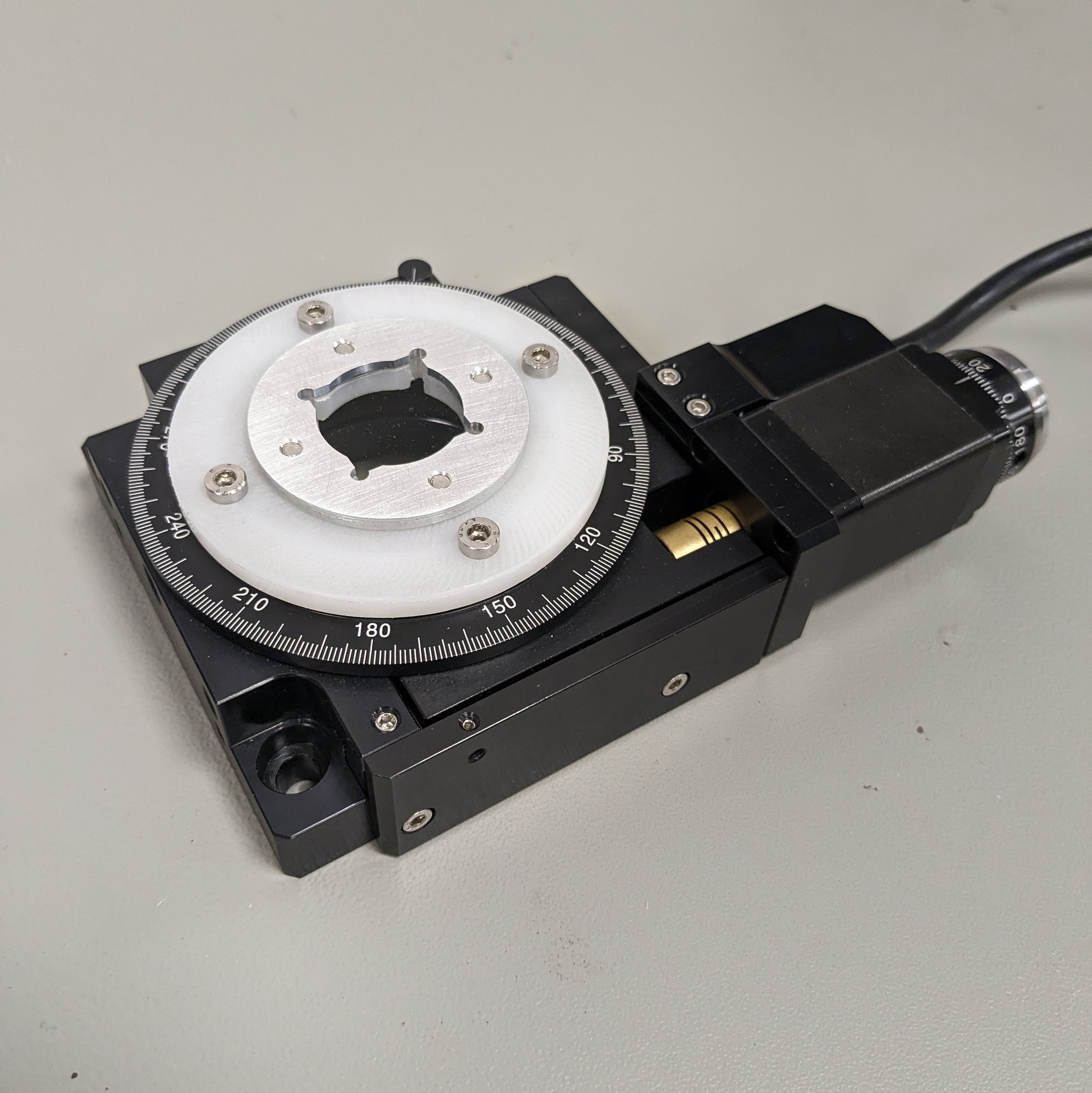
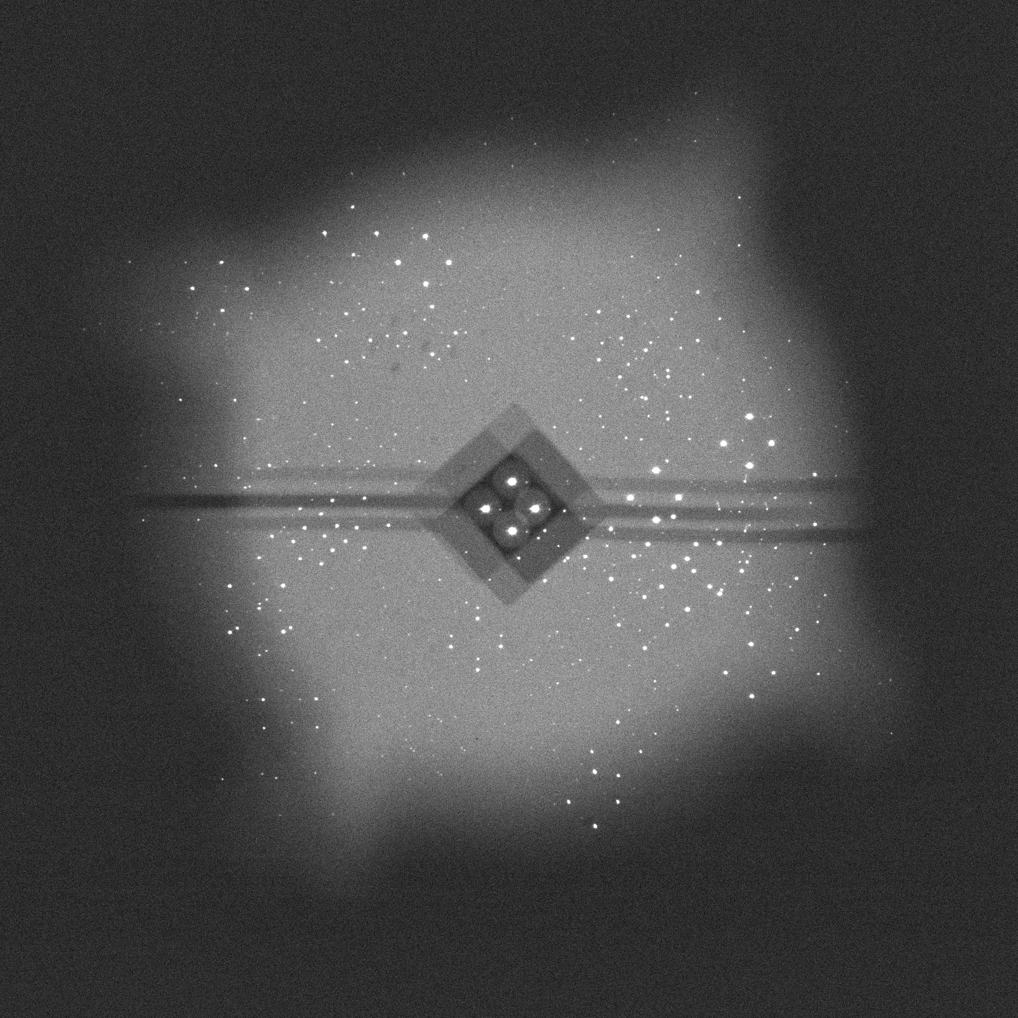
The calibrator system for RoboPol presented in this paper consists of half-wave plate (HWP) made of quartz and MgF2 crystals that is then mounted on a Standa rotary stage (Part# 8MR190-2-28). The HWP is optimized for performance in the optical wavelengths of , which encompasses all the broadband filters of RoboPol. The mounting adapters to place the HWP on the rotary stage is either 3-D printed or made in local machining workshops in Crete. A picture of the calibrator system is shown in Figure 2(a). The rotary stage is controlled by a Controller Box developed in-house by the lab at Inter-University Centre for Astronomy and Astrophysics (IUCAA), Pune, India. The calibrator system is mounted on top of the RoboPol instrument, just ahead of the focal plane/mask plane. The aperture of the HWP used is 25 mm 25 mm, smaller than the nominal FoV size at the telescope focal plane. The size of the HWP in combination with the mounting system vignettes light from regions at outer part of the original RoboPol FoV. The obtained FoV with the HWP calibrator is roughly ; an image obtained from RoboPol with the calibrator system mounted on it is shown in Figure 2(b).
3 Observations and Analysis
To test the on-sky performance of the calibrator system, it was mounted on RoboPol, and observations were carried out for a sample of unpolarized and polarized standard stars traditionally used for RoboPol observations. Table 1 and 2 list all the standard star measurements conducted for this project. To estimate the long-term performance with this system, measurements were taken on 5 nights spread over 2 RoboPol observing seasons. As noted earlier, each observation consists of one or multiple sets of four exposures with RoboPol at HWP positions of , , , and with respect to the ICS.
For the analysis of the raw data, an automated data reduction pipeline was developed using the Python programming language. Attention was given towards error estimation and propagation in each step of the analysis. Photometry was performed using the aperture photometry package of the Photutils software222https://photutils.readthedocs.io/en/stable/. Curve of growth plots were created for each image, and appropriate aperture and annulus radii were chosen. Using this procedure, the intensities and were obtained for all HWP positions. Differential transmission for the and beams, characterized by the correction factors and (as given by Equations 5 and 6), was calculated. Subsequently, the beam intensity was corrected as . The normalized Stokes number is then given by the normalized difference between the two intensities, as given by Equation 7.
and are the Stokes parameter values from the two Halfs of RoboPol that corresponds to either or , depending on the HWP position , as given by Equations 8 and 9, where the subscripts and correspond to the left and right Half measurements. The overall and are found using the Equations 10 and 11 and the associated uncertainty in the measurements is found by taking the standard deviation of the corresponding values.
| (7) |
| (8) |
| (9) |
| (10) |
| (11) |
| Source Id | Filter Used | Date of Observation |
| BD+32.3739 | R | Jun 8, 2022 |
| Jul 1, 2023 | ||
| Jul 2, 2023 | ||
| Nov 15, 2023 | ||
| BD+32.3739 | R | Jul 1, 2023 |
| Jul 2, 2023 | ||
| BD+32.3739 | B | Jun 8, 2022 |
| Jul 1, 2023 | ||
| Jul 2, 2023 | ||
| Nov 15, 2023 | ||
| BD+32.3739 | B | Jul 1, 2023 |
| Jul 2, 2023 | ||
| BD+32.3739 | I | Jul 1, 2023 |
| Jul 2, 2023 | ||
| BD+28.4211 | R | Jul 1, 2023 |
| Nov 15, 2023 | ||
| Nov 15, 2023 | ||
| BD+28.4211 | B | Nov 15, 2023 |
| Nov 15, 2023 | ||
| BD+40.2704 | R | Jun 8, 2022 |
| BD+40.2704 | Jun 8, 2022 | |
| HD212311 | R | Jul 1, 2023 |
| Nov 15, 2023 | ||
| HD212311 | B | Nov 15, 2023 |
| Source Id | Filter Used | Date of Observation |
|
|
||||
| HD155197 | R | Jul 1, 2023 | 4.986 | 102.88 | ||||
| HD155528 | R | Jul 1, 2023 | 5.21 | 92.61 | ||||
| Hiltner960 | R | Jul 1, 2023 | 5.21 | 54.54 | ||||
| Jul 2, 2023 | 5.21 | 54.54 | ||||||
| Nov 15, 2023 | 5.8 | 54.54 | ||||||
| HD183143 | R | Jun 8, 2022 | 5.8 | 178.6 | ||||
| Nov 15, 2023 | ||||||||
| HD183143 | B | Jun 8, 2022 | 5.8 | 178.6 | ||||
| Nov 15, 2023 | ||||||||
| HD183143 | I | Jun 8, 2022 | 3.13 | 178.6 | ||||
| CygOB2 | R | Jun 8, 2022 | 3.13 | 86 | ||||
| Nov 15, 2023 | ||||||||
| CygOB2 | R | Nov 15, 2023 | 4.893 | 86 | ||||
| HD204827 | R | Nov 15, 2023 | 5.648 | 59.1 | ||||
| HD204827 | B | Nov 15, 2023 | 5.648 | 58.2 |
4 Results
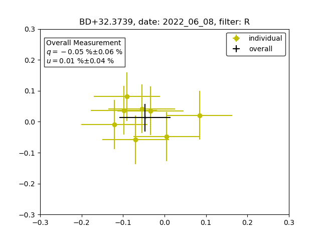
Figure 3 is a plot of the polarimetric measurement of a single unpolarized standard star BD+32.3739 in the SDSS-r filter. As noted above, we get 2 measurements of and from each half of RoboPol, thus 4 values in total per cycle. For the observation in Figure 3, 2 sets of such measurements were done. From the mean and variance, we get the overall polarization of the source and the associated standard deviation. As can be noted, the final values of and are completely corrected for instrumental polarization through the modulating effect of the calibrator HWP; there is no residual measured polarization within the values of the spread of measurements ( 0.05 %).
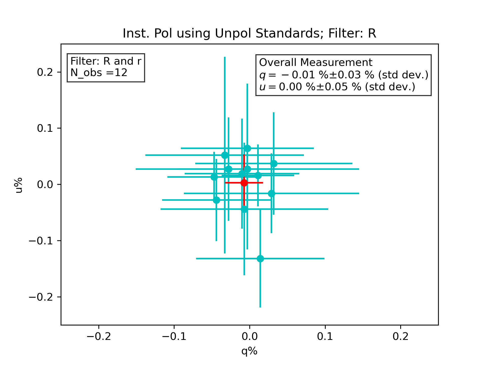
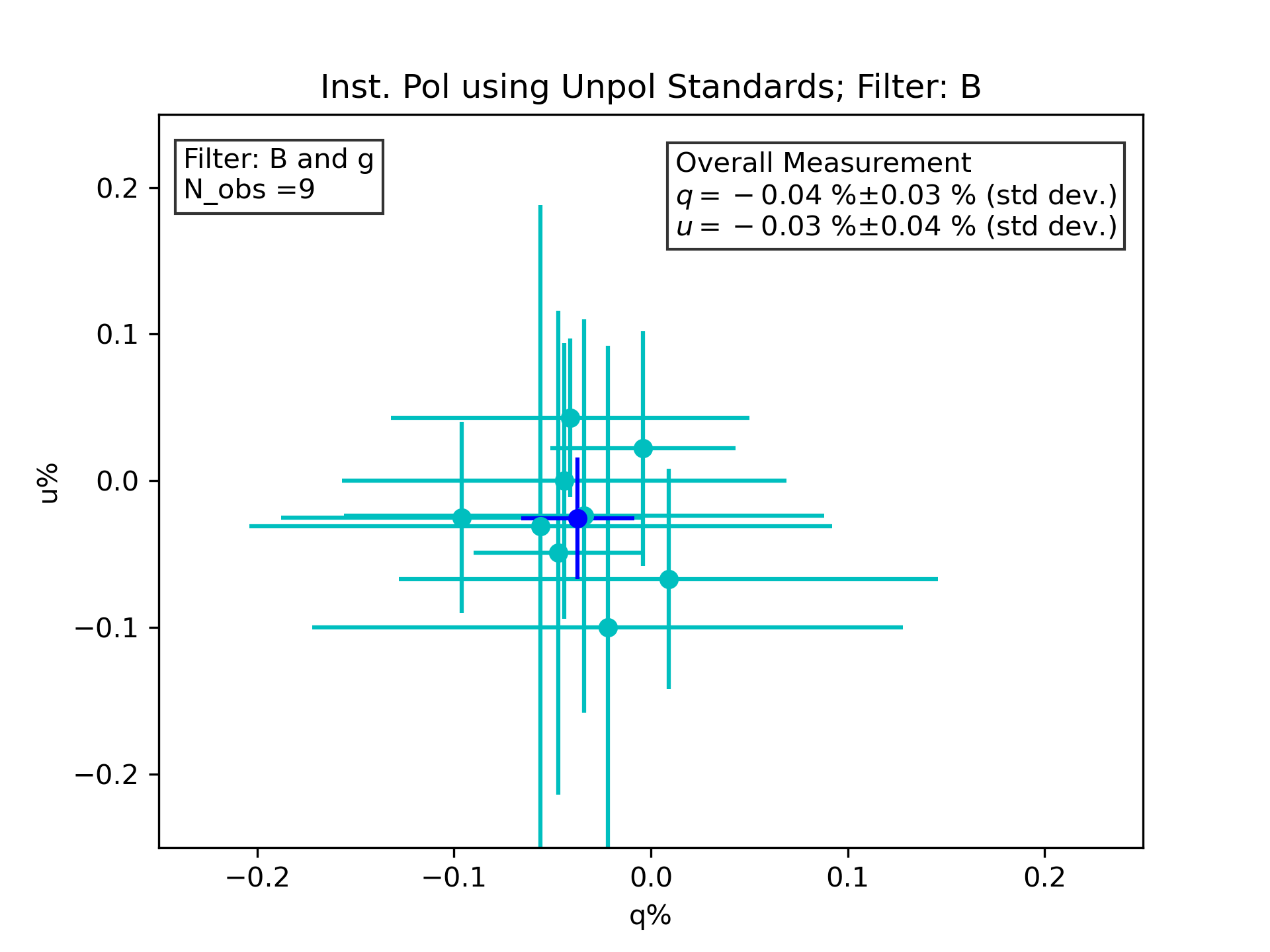
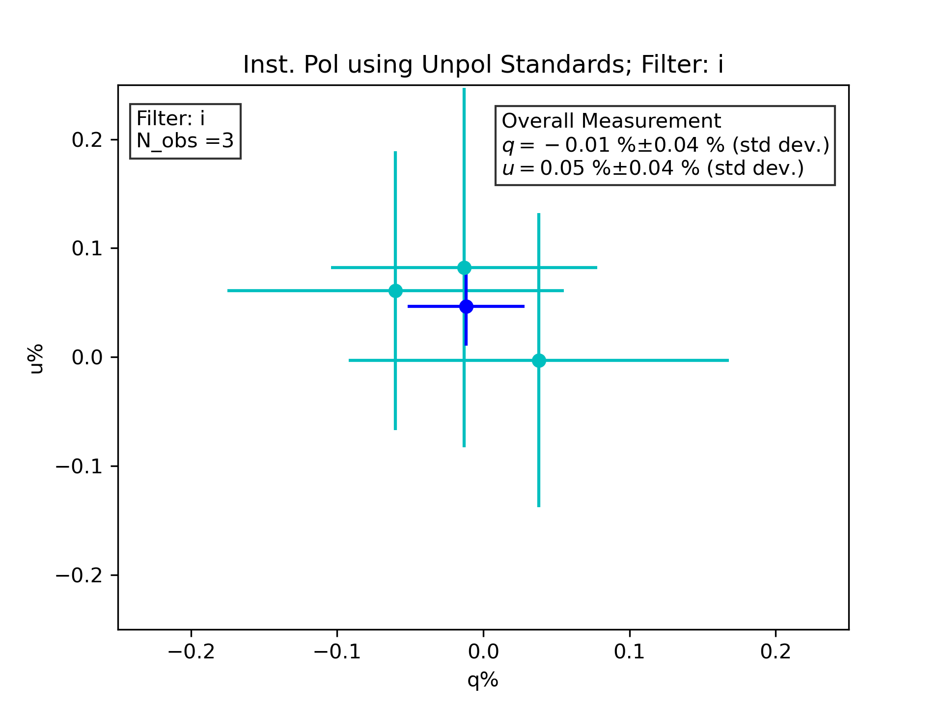
To quantify the long-term accuracy and sensitivity of the instrument with the calibrator, measurements of all the unpolarized standards stars are collated for each filter. Without segregating as a function of date or season, the overall results are shown in Figure 4. As can be seen through the plots, for each filter, the accuracy in and is better than 0.05 % in both and . Equally importantly, the absolute value of instrumental polarization is zero within measurement uncertainties. Please note that in this accuracy regime, a small or significant part of the variance seen in the measurements will be originating from the variability and non-zero value of the standard unpolarized stars used for calibration themselves.
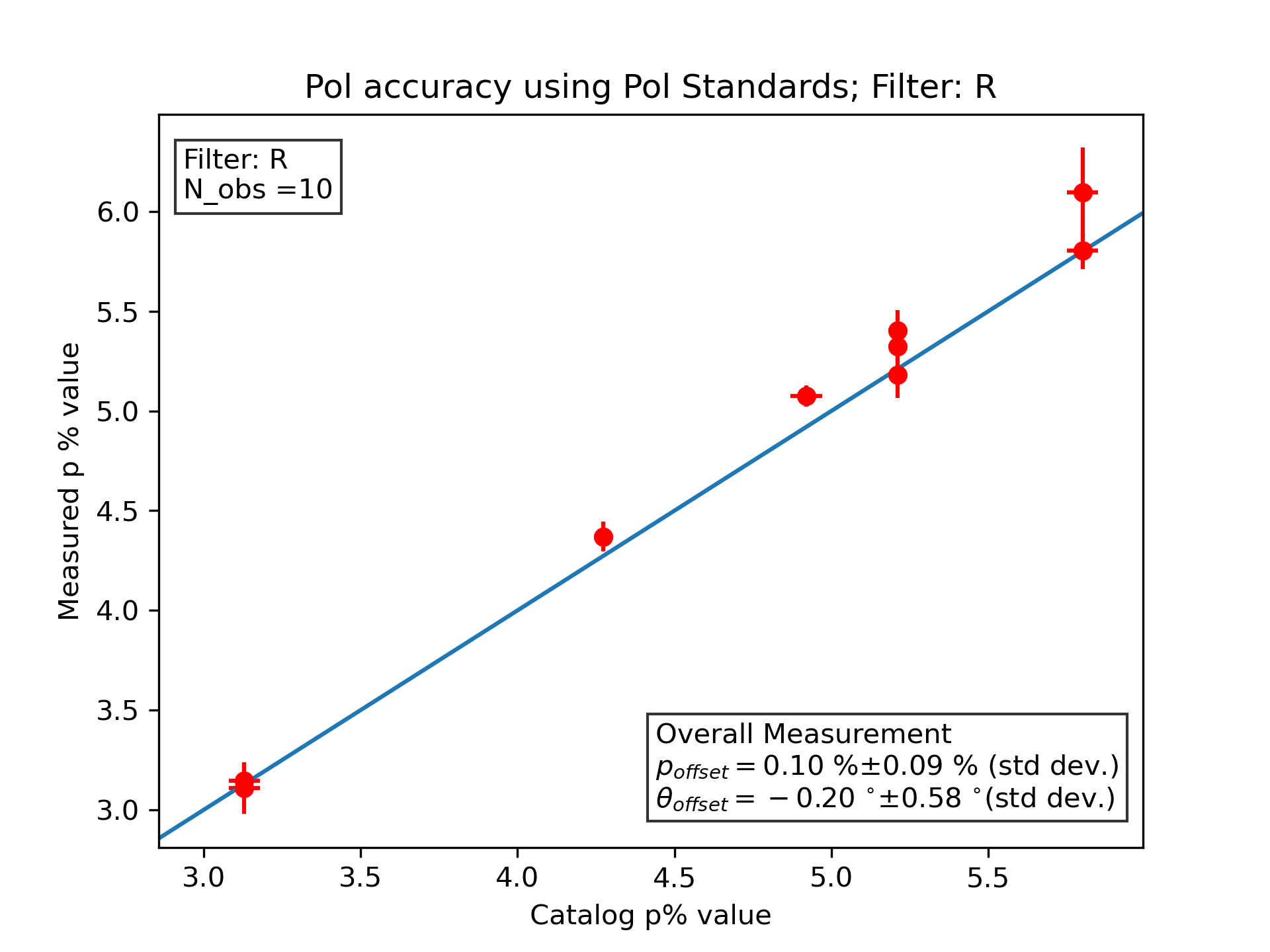
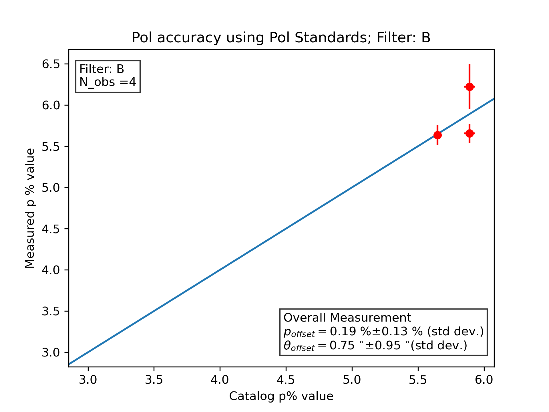
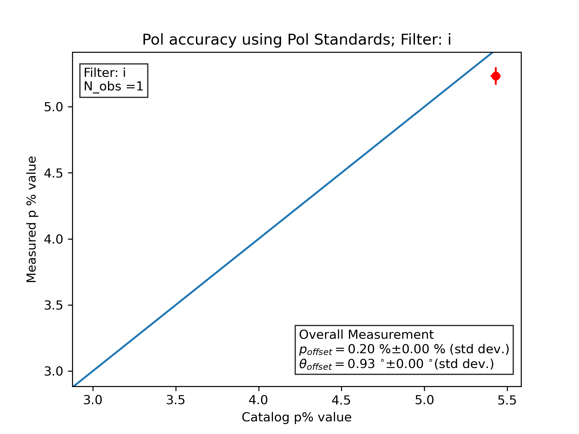
Figure 5 plots the instrument-measured polarization values, , in comparison to the standard polarized stars used in the polarimetry community. In the R band, it can be noted that the measured fractional polarization values match the catalog values to better than 0.1 % accuracy. Furthermore, the measured polarization angle matches the catalog value to better than in the R band after correction for the instrument’s rotation. This represents an improvement by a factor of 2. More measurements are needed in the B and I bands to make a robust claim for these filters.
5 Conclusions
Table 3 compares the performance of the new calibrator system with the normal RoboPol mode. There are two key improvements. Firstly, in just the R band, there is at least a two-fold improvement in the accuracy of the instrument (), as well as better matching with catalog polarization values of standard stars. Secondly, the HWP calibrator improves the accuracy in all broadband filters, which will enable RoboPol to carry out new scientific studies that require high accuracy multi-filter polarimetric studies. An example of such research includes the measurement of Serkowski curves along the ultra-diffuse interstellar medium sightlines, where dust-induced polarization is typically very low, at levels of or lower. Prior to the implementation of the HWP calibrator, RoboPol was limited in its ability to accurately measure this phenomenon, often only able to provide upper limits on the signal due to constraints imposed by instrument accuracy.
| Filter | Instrumental polarization with calibrator | Instrumental polarization without calibrator |
|---|---|---|
| B | 0.05% 0.03% | 0.29% 0.16% |
| R | 0.01% 0.03% | 0.30% 0.09% |
| I | 0.05% 0.04% | 0.60% 0.08% |
Acknowledgements.
The PASIPHAE program is supported by grants from the European Research Council (ERC) under grant agreement No 771282 and No 772253, from the National Science Foundation, under grant number AST-1611547 and AST-2109127, and the National Research Foundation of South Africa under the National Equipment Programme. This project is also funded by an infrastructure development grant from the Stavros Niarchos Foundation and from the Infosys Foundation. K.T. acknowledges support from the Foundation for Research and Technology – Hellas Synergy Grants Program through project POLAR, jointly implemented by the Institute of Astrophysics and the Institute of Computer Science. We thank Anna Steiakaki for her help in various phases of the project, including component fabrication and installation on the telescope.Appendix A Measured Stokes Parameters and Instrument Matrix
The incident intensity at the detector for any polarization channel of the instrument (, , and polarizations) can be written as:
| (12) |
where , and correspond to the elements of the first row of the Mueller matrix for the optical path corresponding to that polarization angle/channel. The normalized difference between intensities corresponding to two orthogonal polarization angles/channels yields or , as given by the following equation.
| (13) |
The binomial expansion of is given by . Using that, the generalized normalized difference can be written as a polynomial equation in and .
| (14) |
In general, for most simple polarimeters, the second order terms are zero, and the instrument measured Stokes parameters can be written as a set of linear equations, together forming a Muller matrix like Instrument Matrix. The first row is inconsequential to polarimetric measurements and hence can be ignored.
| (15) | |||
| (16) |
References
- [1] Ramaprakash, A. N., Rajarshi, C. V., Das, H. K., Khodade, P., Modi, D., Panopoulou, G., Maharana, S., Blinov, D., Angelakis, E., Casadio, C., Fuhrmann, L., Hovatta, T., Kiehlmann, S., King, O. G., Kylafis, N., Kougentakis, A., Kus, A., Mahabal, A., Marecki, A., Myserlis, I., Paterakis, G., Paleologou, E., Liodakis, I., Papadakis, I., Papamastorakis, I., Pavlidou, V., Pazderski, E., Pearson, T. J., Readhead, A. C. S., Reig, P., Słowikowska, A., Tassis, K., and Zensus, J. A., “RoboPol: a four-channel optical imaging polarimeter,” Monthly Notices of the Royal Astronomical Society 485, 2355–2366 (02 2019).
- [2] King, O. G., Blinov, D., Ramaprakash, A. N., Myserlis, I., Angelakis, E., Baloković, M., Feiler, R., Fuhrmann, L., Hovatta, T., Khodade, P., Kougentakis, A., Kylafis, N., Kus, A., Modi, D., Paleologou, E., Panopoulou, G., Papadakis, I., Papamastorakis, I., Paterakis, G., Pavlidou, V., Pazderska, B., Pazderski, E., Pearson, T. J., Rajarshi, C., Readhead, A. C. S., Reig, P., Steiakaki, A., Tassis, K., and Zensus, J. A., “The RoboPol pipeline and control system,” Monthly Notices of the Royal Astronomical Society 442, 1706–1717 (06 2014).
- [3] Blinov, D., Kiehlmann, S., Pavlidou, V., Panopoulou, G. V., Skalidis, R., Angelakis, E., Casadio, C., Einoder, E. N., Hovatta, T., Kokolakis, K., Kougentakis, A., Kus, A., Kylafis, N., Kyritsis, E., Lalakos, A., Liodakis, I., Maharana, S., Makrydopoulou, E., Mandarakas, N., Maragkakis, G. M., Myserlis, I., Papadakis, I., Paterakis, G., Pearson, T. J., Ramaprakash, A. N., Readhead, A. C. S., Reig, P., Słowikowska, A., Tassis, K., Xexakis, K., Żejmo, M., and Zensus, J. A., “RoboPol: AGN polarimetric monitoring data,” Monthly Notices of the Royal Astronomical Society 501, 3715–3726 (12 2020).
- [4] Mandarakas, N., Blinov, D., Aguilera-Dena, D. R., Romanopoulos, S., Pavlidou, V., Tassis, K., Antoniadis, J., Kiehlmann, S., Lychoudis, A., and Tsemperof Kataivatis, L. F., “GRB 210619B optical afterglow polarization,” A&A 670, A144 (Feb. 2023).
- [5] Pelgrims, V., Mandarakas, N., Skalidis, R., Tassis, K., Panopoulou, G. V., Pavlidou, V., Blinov, D., Kiehlmann, S., Clark, S. E., Hensley, B. S., Romanopoulos, S., Basyrov, A., Eriksen, H. K., Falalaki, M., Ghosh, T., Gjerløw, E., Kypriotakis, J. A., Maharana, S., Papadaki, A., Pearson, T. J., Potter, S. B., Ramaprakash, A. N., Readhead, A. C. S., and Wehus, I. K., “The first degree-scale starlight-polarization-based tomography map of the magnetized interstellar medium,” A&A 684, A162 (2024).
- [6] Skalidis, R., Panopoulou, G. V., Tassis, K., Pavlidou, V., Blinov, D., Komis, I., and Liodakis, I., “Local measurements of the mean interstellar polarization at high galactic latitudes,” A&A 616, A52 (2018).
- [7] Panopoulou, G. V., Hensley, B. S., Skalidis, R., Blinov, D., and Tassis, K., “Extreme starlight polarization in a region with highly polarized dust emission,” A&A 624, L8 (Apr. 2019).
- [8] Blinov, D., Maharana, S., Bouzelou, F., Casadio, C., Gjerløw, E., Jormanainen, J., Kiehlmann, S., Kypriotakis, J. A., Liodakis, I., Mandarakas, N., Markopoulioti, L., Panopoulou, G. V., Pelgrims, V., Pouliasi, A., Romanopoulos, S., Skalidis, R., Anche, R. M., Angelakis, E., Antoniadis, J., Medhi, B. J., Hovatta, T., Kus, A., Kylafis, N., Mahabal, A., Myserlis, I., Paleologou, E., Papadakis, I., Pavlidou, V., Papamastorakis, I., Pearson, T. J., Potter, S. B., Ramaprakash, A. N., Readhead, A. C. S., Reig, P., Słowikowska, A., Tassis, K., and Zensus, J. A., “The robopol sample of optical polarimetric standards,” A&A 677, A144 (2023).
- [9] Maharana, S., Kiehlmann, S., Blinov, D., Pelgrims, V., Pavlidou, V., Tassis, K., Kypriotakis, J. A., Ramaprakash, A. N., Anche, R. M., Basyrov, A., Deka, K., Eriksen, H. K., Ghosh, T., Gjerløw, E., Mandarakas, N., Ntormousi, E., Panopoulou, G. V., Papadaki, A., Pearson, T., Potter, S. B., Readhead, A. C. S., Skalidis, R., and Wehus, I. K., “Bright-moon sky as a wide-field linear polarimetric flat source for calibration,” A&A 679, A68 (2023).
- [10] Mandarakas, N., Panopoulou, G. V., Pelgrims, V., Potter, S. B., Pavlidou, V., Ramaprakash, A., Tassis, K., Blinov, D., Kiehlmann, S., Koutsiona, E., Maharana, S., Romanopoulos, S., Skalidis, R., Vervelaki, A., Clark, S. E., Kypriotakis, J. A., and Readhead, A. C. S., “Zero-polarization candidate regions for the calibration of wide-field optical polarimeters,” A&A 684, A132 (2024).
- [11] Tinyanont, S., Millar-Blanchaer, M., Jovanovic, N., Mawet, D., Vasisht, G., Milburn, J. W., Serabyn, E., Porter, M., Palatnick, S., and Hopkins, C., “Achieving a spectropolarimetric precision better than 0.1 % in the near-infrared with WIRC+Pol,” in [Polarization Science and Remote Sensing IX ], Craven, J. M., Shaw, J. A., and Snik, F., eds., 11132, 1113209, International Society for Optics and Photonics, SPIE (2019).
- [12] Ramaprakash, A. N., Gupta, R., Sen, A. K., and Tandon, S. N., “An imaging polarimeter (impol) for multi-wavelength observations,” Astron. Astrophys. Suppl. Ser. 128(2), 369–375 (1998).