The Stochastic Gravitational Wave Background from Primordial Gravitational Atoms

Abstract

We propose a scenario of primordial gravitational atoms (PGAs), which may exist in the current and past universe due to spinning primordial black holes (PBHs) and very light bosonic fields. In a monochromatic mass scenario with a sizable dimensionless spin, which may arise in a short matter dominated (MD) era, we analyze the resulting stochastic gravitational wave background (SGWB) signal. Its spectrum is approximately characterized by a rising $\propto f^{3}$ followed by a falling $\propto f^{-1}$ where $f$ is the frequency. Then, we investigate the constraints and prospects of such a SGWB, and find that PGAs with a core mass $M_{\rm BH}\sim{\cal O}(10)~{}M_{\odot}$ and a cloud of light scalar with mass $\mu\sim{\cal O}(10^{-13})$ eV could yield constraints even stronger than those from bare PBHs. Future detectors such as LISA, Taiji and TianQin are able to explore PGAs over a narrow and elongated strap in the $(\mu,M_{\rm BH})$ plane, spanning over 10 orders of magnitude for the maximum spin, $10^{-8}~{}M_{\odot}\lesssim M_{\rm BH}\lesssim 10^{4}~{}M_{\odot}$, $10^{-16}~{}{\rm eV}\lesssim\mu\lesssim 10^{-3}~{}\rm eV$. If the PGA is dressed with a vector cloud, the SGWB signal has a much better opportunity to be probed.

1 Introduction

The superradiance of rotating black holes (Kerr black holes) is a particularly intriguing phenomenon. Bosonic waves incident on a black hole satisfying the superradiance condition ($\omega<m\Omega_{H}$, where $\omega$ is the wave frequency, $m$ is the wave’s angular frequency, and $\Omega_{H}$ is the black hole’s angular velocity) will extract energy and angular momentum from the black hole, enhancing the reflected waves. Brito et al. provided a comprehensive review of the superradiance phenomenon in Ref. [1]. Based on it, Press and Teukolsky proposed the concept of superradiant instability [2, 3]. Imagine a scenario where the black hole is enveloped by a reflective mirror. Bosonic waves satisfying the superradiance condition would be trapped between the black hole and its mirror, continuously reflecting and thereby extracting energy from the black hole, enhancing the wave’s energy. Considering practical scenarios, if there exist massive bosonic waves that satisfy the superradiance condition, gravity would act as a mirror, confining the bosonic waves near the black hole and forming quasi-normal bound states [4, 5, 6, 7, 8, 9, 10, 11, 12, 13, 14, 15]. We refer to these bound states as ”bosonic clouds” and designate the black holes enveloped by boson clouds as ”gravitational atoms (GAs)”. Bosonic clouds can radiate gravitational waves (GWs), providing a means to detect bosons, as reviewed in [16].

It is of great interest to consider that the core of the GA is a primordial black hole (PBH), which is believed to be relics of the early universe inhomogeneities [17, 18, 19, 20] . Therefore, primordial gravitational atoms (PGAs) convey information about the early universe encoded in the stochastic gravitational wave background (SGWB). One immediate piece of information is on the spin of PBHs. In the standard cosmology, PBHs only formed in the radiation-dominated (RD) era. The details of the standard scenario is discussed in Ref. [29] and references therein. It is widely believed that PBHs usually carry little spin, namely the dimensionless spin parameter $\tilde{a}\equiv\frac{M_{\rm PL}^{2}}{M_{\text{BH}}^{2}}J_{\text{BH}}\lesssim 0.01$, with $J_{\text{BH}}$ the angular momentum of the black hole [30, 31, 32], making it difficult for them to exhibit superradiance.

The situation becomes different in non-standard scenarios, including both the non-standard origins of inhomogeneities other than the primordial quantum fluctuations during the inflation stage, as well as the non-standard phases of the early universe. Many scenarios of PBH formation are reviewed in Refs. [21, 28]. In most scenarios, their spins are not clear, but there are still some hopeful cases which may give rise to a sizable $\tilde{a}$. For instance, it is shown that PBHs from collapsing domain walls may have $\tilde{a}\lesssim 0.1$ only for $M_{\rm BH}\gtrsim 10^{-3}M_{\odot}$, whereas less massive black holes receive extreme spins $\tilde{a}\simeq 1$ [33]. A well-known example is from the overdensity collapsing to PBHs during the pressureles matter-dominated (MD) era, where collapse is more prone to be anisotropic and their spins are typically large, even approaching 1 [34]. But this study does not take into account matter accretion, which may play an important role in black hole formation and growth [35]. Numerical relativistic studies focus on this topic [36]. Finally, mergers of PBHs may also results in a spinning remnant [37]. Therefore, it makes sense to study the possible signals of superradiance associated with PGAs, which are distinguished from those associated with the astronomical GAs.

Actually, during the progress of this project, several works studying the same topic already appeared, but they focus on different aspects of the PGAs. Pani and Loeb [38] investigated PBHs surrounded by photon clouds. During the RD era, PBHs are enveloped by plasma, which imparts an effective mass to photons, resulting in the formation of PGAs. Considering the impact of photon clouds on the CMB, they placed constraints on the abundance of PBHs in the mass range of $10^{-8}M_{\odot}$ to $10^{0.2}M_{\odot}$. The constraints depend on the average initial spin of the PBHs, $\langle\tilde{a}\rangle$. Ferraz et al. [39] investigated the electromagnetic signals produced by pion clouds around very light PBHs of mass $M_{\text{BH}}\sim 10^{-18}M_{\odot}$. They found that efficient pion production is only possible for $\tilde{a}\gtrsim 0.8-0.9$, to overcome both neutral pion decay and charged pion annihilation. Branco et al. [40] considered axion clouds with self-interactions, generated around asteroid-mass PBHs, which could constitute all dark matter. They found that a significant number of axions could escape from the bound states into the intergalactic medium or host galaxy, potentially contributing to the galactic and extragalactic background flux. By considering two specific cases with $\tilde{a}=0.01$ and $\tilde{a}=0.99$, they constrained the coupling constant of photons with $20~{}\text{eV}-10^{6}~{}\text{eV}$ axions. Recently, Dent et al. [41] also focused on these PGAs, conducting their research using multi-messenger probes. However, gravitational signal was not discussed until a very recent work [42], which considered the merger of two equal-mass PBHs produced in first order of phase transition, resulting in a PGA with $\tilde{a}\sim 0.67$. Then, the authors studied GWs from clouds transitions between different energy levels.

Our focus is also the GW signal from PGAs, but our strategy differs from Ref. [42], and our goal is to explore the general features and its potential at detectors of such signals. In this paper, we consider a scenario where PBHs formed during a short MD era coexist with a real scalar or vector field in the universe. Adopting a conservative approach, we assume that the bosonic field only engages in gravity-related interactions and does not couple with other particle fields. In this context, we calculate the SGWB spectrum radiated by superradiant clouds surrounding PBHs, to find that it is approximately characterized by a rising $\propto f^{3}$ followed by a falling $\propto f^{-1}$ where $f$ is the frequency. Using such a spectrum, the current data is able to place constraints on the abundance of these PBHs within the parameter space defined by the bosonic field mass $\mu$ and the mass of the PBHs $M_{\rm BH}$. The constraints can be even stronger than that made using bare PBHs. At the future detectors such as LISA, Taiji and TianQin, in which a wide scalar cloud PGA population has the potential to leave imprints, roughly over $10^{-8}~{}M_{\odot}\lesssim M_{\rm BH}\lesssim 10^{4}~{}M_{\odot}$, $10^{-16}~{}{\rm eV}\lesssim\mu_{S}\lesssim 10^{-3}~{}\rm eV$ for . The spin of vector boson matters, significantly boosting the discovery potential of PGAs with a vector cloud.

The work is organized as the following: In Section 2 we establish a simple scenario for PGAs. In Section 3 we calculate the SGWB spectrum from PGAs, and moreover analyze the current constraints on it and as well its prospects. In the appendix we review the key details of PBHs formed in a,MD era. The final section includes the conclusions and discussions.

2 PBH in the Monochromatic Mass Scenario

The mass spectrum and spin distribution of PBHs, depend on their production mechanism, late accretion and even their cosmic evolution [43], so it is quite complicated to make a comprehensive understanding, which is beyond the scope of this work. Although the actual mass spectrum of PBHs is extended, for specific cases such as primordial fluctuations peaking around a certain scale and the short MD era sceanario considered next, the PBH mass can be approximated by a monochromatic spectrum. To simplify the problem, we first study the case where the PBH mass follows a monochromatic distribution, which allows for a tentative study of the GW signals from PGAs.

In this paper, we consider a realistic scenario where PBHs are produced during a short MD era, and their spin distribution will be provided. Additionally, we will consider that the PBH mass and spin take fixed values $M_{\rm BH}$ and $\tilde{a}$ respectively, without targeting any specific formation scenario.

2.1 Monochromatic PBHs from a Short MD Era

Unlike the formation scenario of PBHs during the RD era, where pressure plays a major role, the PBH formation during a MD era is primarily related to the anisotropy of the collapse. This has been studied in Ref. [44]. Furthermore, Harada et al. [34] investigated the effects of the PBH spin on PBH formation, and they also found the non-dimensional spins are typically large, even approaching 1. Ref. [45] examined the impact of inhomogeneity. Recently, Ref. [46] studied the impacts of velocity dispersion. For numerical relativistic studies, see [36]. In order not to interfere with the main line of the article, we will include a review of the details in the Appendix A, and in the following we just quote the key formulas.

In standard cosmology, the sole MD started at the time corresponding to matter-radiation equality. Since there is no observational data to constrain the thermal history of the universe before big bang nucleosynthesis (BBN) [47, 48], various models of an early MD era before BBN exist. These models include the domination of nonrelativistic particles [49, 50, 51, 52, 53], the existence of moduli fields in string theory models [54, 55], and the end of inflation [56, 57, 58, 59, 60, 61, 62]. We consider an early MD era lasts from $t_{\text{ini}}$ to $t_{\text{end}}$, during which the Hubble constant $H$ and scale factor $a$ respectively behave as

$$H=\frac{2}{a_{m}\eta^{3}}=2a_{m}^{1/2}a^{-3/2}=\frac{2}{3t}~{}(t_{\text{ini}}<t<t_{\text{end}}),\quad a(t)=a_{m}\eta^{2}=a_{m}^{1/3}(3t)^{2/3},$$ (2.1)

with $a_{m}$ the integral constant determined by matching at $t_{\rm end}$ and $\eta$ the conformal time. Subsequently, these dominant matter would decay into high-energy particles as radiation, recovering the RD era. We assume that this happens instantly, and then the reheating temperature $T_{\text{rh}}$ is determined by energy conservation, $\rho(t_{\text{end}})=\rho_{r}(t_{\text{end}})$, giving $T_{\text{rh}}=\left({30}/{\pi^{2}g_{*}}\right)^{1/4}\rho(t_{\text{end}})^{1/4}$, where $g_{*}$ is the radiation degree of freedom after $t=t_{\text{end}}$. After reheating, the universe undergoes adiabatic expansion, and then both the energy density of PBH (behaving as matter) and entropy density scale as $a^{-3}$, so the ratio $\rho_{\text{PBH}}(t>t_{\text{end}})/s(t>t_{\text{end}})$ keeps constant.

In this paper, we consider PBHs formed from the collapse of primordial fluctuations after crossing the horizon, with masses approximately equaling to the Hubble mass at the horizon-crossing. According to the discussion in Appendix A.1, for a long MD era, the mass range of PBHs is given by

$$M_{H}(t_{\rm ini})\lesssim M_{\rm BH}\lesssim M_{H}(t_{\text{end}})\sigma_{\text{max}}^{3/2},$$ (2.2)

where $\sigma_{\rm max}\equiv\sigma_{H}(k_{\rm max})$, and $k_{\rm max}$ denotes the mode collapsing at $t_{\rm end}$. Let us consider a short MD era scenario where $M_{H}(t_{\rm ini})\simeq M_{H}(t_{\text{end}})\sigma_{\text{max}}^{3/2}$, which implies that the mass spectrum is monochromatic and only the mode $k_{\rm max}$ can collapse into PBHs.

We arrange such an artificial setup is to control the possible reduction of $\tilde{a}$ owing to matter accretion. Recently, Ref. [63] found that, the dimensionless spin $\tilde{a}$ reaches its peak after $\sim 1$e-fold of collapse initiation. Then, $\tilde{a}$ suffers a fast reduction within $\sim 1$e-fold due to the accretion of non-rotating matter . A short MD era does not allow PBH to significantly accrete. Then, the corresponding PBH energy fraction approximately is given by [45]

$$\frac{\rho_{\rm PBH}({t_{\rm end}})}{\rho({t_{\rm end}})}=\beta(k_{\rm max})\simeq 0.2055\sigma_{\rm max}^{13/2},$$ (2.3)

where $\beta(k_{\rm max})$ represents the probability of perturbations at the scale $k_{\max}$ collapsing into PBHs. For further details, please refer to Appendix A.

Otherwise, in the case with a long MD era, only the PBHs produced near the end of MD era is of our interest. But that requires a specific study on the constraints on the extended spectrum. Anyway, a more rigorous treatment for the general situation requires the details of the primordial perturbation power spectrum and as well the beginning and end of the MD era. In the current work, we take the simplifying setup above and leave the latter for a future study.

Moreover, for the setup we considered, the accretion effect can be ignored and then we assume that the spin distribution is given by [34] .

$$P_{2}(\tilde{a})\propto\frac{1}{\tilde{a}^{5/3}}\exp\left(-\frac{1}{2\sigma_{\text{max}}^{2/3}}\left(\frac{2}{5}I\right)^{4/3}\frac{1}{\tilde{a}^{4/3}}\right),$$ (2.4)

which requires that the initial shapes of those overdense regions collapsing into PBHs are very close to spherical. $I$ is a dimensionless constant related to the perturbation power spectrum and we take $I=1$. For a detailed discussion on the production rate of PBHs and their spin distribution, see the Appendix A.2. Actually, the limit of monochromatic spectrum allows us to fully determine the above spin distribution of PBHs in terms of two observables, $M_{\rm BH}$ and $f_{\rm PBH}$, as shown below.

The key is to express the variance $\sigma_{\text{max}}$ in terms of $M_{\rm BH}$ and $f_{\rm PBH}$. To that end, we first use the radiation energy relation $\rho(t_{\rm end})=3s(t_{\rm end})T_{\rm rh}/4$ to get

$$\beta =\frac{\rho_{\text{PBH}}(t_{\text{end}})}{\rho(t_{\text{end}})}=\frac{4}{3T_{\text{rh}}}\frac{\rho_{\text{PBH}}(t_{\text{end}})}{s(t_{\text{end}})}=\frac{4}{3T_{\text{rh}}}\frac{f_{\text{PBH}}\rho_{\text{DM}}}{s|_{\rm present}},$$ (2.5)

where $\rho_{\rm PBH}|_{\rm present}=\rho_{\text{DM}}f_{\text{PBH}}$, and $\rho_{\text{DM}}$ is the dark matter energy density at present. The reheating temperature can also be expressed in terms of the PBH mass and $\sigma_{\text{max}}$ as

$$T_{\text{rh}} =\left(\cfrac{45}{4\pi^{3}g_{*}}\right)^{1/4}M_{\rm PL}^{1/2}H(t_{\text{end}})^{1/2}=\left(\cfrac{45}{4\pi^{3}g_{*}}\right)^{1/4}M_{\rm PL}^{1/2}M_{\rm PL}(2M_{\text{BH}})^{-1/2}\sigma_{\text{max}}^{3/4},$$ (2.6)

where we have used the relation Eq. (A.3) to express $H(t_{\text{end}})$. Substituting it into Eq. (2.5), we get a relation of the PBH formation probability and the PBH abundance

$$\beta=2.6681\times 10^{-9}\left(\frac{g_{*}}{106.75}\right)^{1/4}f_{\text{PBH}}\left(\frac{M_{\text{BH}}}{M_{\odot}}\right)^{1/2}\sigma_{\text{max}}^{-3/4}.$$ (2.7)

Combining Eq. (2.3) with Eq. (2.7), we eventually get the variance as desired

$$\sigma_{\text{max}} \simeq 0.0817f_{\text{PBH}}^{4/29}\left(\frac{g_{*}}{106.75}\right)^{1/29}\left(\frac{M_{\text{BH}}}{M_{\odot}}\right)^{2/29}\simeq 0.0817f_{\text{PBH}}^{4/29}\left(\frac{M_{\text{BH}}}{M_{\odot}}\right)^{2/29}.$$ (2.8)

In fact, the SGWB from PGAs in the short MD era scenario only depends on three parameters $M_{\rm BH}$, $\mu$, and $f_{\rm PBH}$.

Later, we will need the birth time of PBHs $t_{\rm BH}$, approximated to be $t_{\text{end}}$, which is also the beginning of the RD era, and we can estimate it as the following. According to [28], we have

$$\frac{M_{H}(t_{\rm end})}{M_{\odot}}\simeq 2.03\times 10^{5}\left(\frac{t_{\rm end}}{1{\rm s}}\right)=1.7539\times 10^{10}\left(\frac{t_{\rm end}}{\text{1years}}\right).$$ (2.9)

Therefore, we obtain

$$t_{\text{end}} \simeq 5.7016\times 10^{-11}\text{years}\frac{M_{\text{BH}}}{M_{\odot}}\sigma_{\text{max}}^{-3/2}$$

$$\simeq 2.4418\times 10^{-9}\text{years}\times\left(\frac{g_{*i}}{106.75}\right)^{-3/58}f_{\text{PBH}}^{-6/29}\left(\frac{M_{\text{BH}}}{M_{\odot}}\right)^{26/29}.$$ (2.10)

Since the early MD era must end before BBN, thus PBHs must form before 1 second (e.g. $t_{\rm end}\lesssim 1{\rm s}$), which then imposes an upper bound on PBH mass, $M_{\text{BH}}\lesssim 10^{5}M_{\odot}$.

3 The Stochastic GW background from Primordial Gravitational Atoms

The bosonic cloud, once it satisfies the superradiance condition, experiences exponential growth until it reaches saturation. During this growth, the energy and angular momentum of the GA’s core is transferred to the bosonic cloud. After reaching saturation, the bosonic cloud starts to consume its own energy by emitting GWs. Over an extended period, the cloud is eventually depleted. Since each PGA generates GWs, and given the randomness in the spin direction of PBHs and the phase of GWs, the GWs emitted by clouds overlap to form an isotropic and homogeneous SGWB in the universe. The observation of this SGWB can provide insights into the nature of PGAs. For simpilicity, we refer to the PGA clothed in a scalar cloud as PGA-0, and the PGA clothed in a vector cloud as PGA-1.

In this section, We will first provide the necessary details of superradiance and GW radiation for two kinds of PGAs, and then derive and analyze the corresponding spectra of the SGWB, and finally investigate the signals on various current and planned GW detectors.

3.1 Superradiance and GW Radiation: Scalar

3.1.1 The Superradiant Stage: Scalar Cloud Growth

We consider the existence of a real scalar field in the universe, which is assumed to be a free field without interactions except for gravity. We neither do not consider the effect of self-interactions of the scalar field, which may have significant effect [64]. Both aspects are model-dependent.

The dynamics of the free real massive scalar field $\Phi$ in the Kerr spacetime is governed by the Klein-Gordon equation

$$(\nabla^{\mu}\nabla_{\mu}-\mu_{S}^{2})\Phi=0,$$ (3.1)

where $\nabla^{\mu}$ is the covariant derivative operator and $\mu_{S}$ is the mass of the scalar boson. In the Boyer-Lindquist coordinates, $x^{\mu}=[t,r,\theta,\phi]$, the solution can be solved by decomposing it into a linear combination of

$$\Phi_{\omega lm}=e^{-i\omega t}e^{im\phi}S_{lm}(\theta)R_{\omega lm}(r)+c.c.$$ (3.2)

By imposing appropriate boundary conditions, we can obtain solutions representing quasi-bound states. These states can be labeled by $|nlm\rangle$, where $n=1,2,3\ldots$, $l=0,1,\ldots n-1$, and $m=-l,-l+1,\ldots l$. Here $\omega$ is complex in general, with its real part $\omega_{R}$ representing the energy of the state, and its imaginary part $\omega_{I}$, representing the superradiant growth ($\omega_{I}>0$) or the decay ($\omega_{I}<0$); the quantum number $m$ represents the angular momentum of the state along the direction of the black hole spin. The gravitational fine-structure parameter, which is defined as $\alpha\equiv\mu_{S}M_{\text{BH}}/M_{\rm PL}^{2}=0.75(M_{\text{BH}}/M_{\odot})(\mu_{S}/10^{-10}eV)$, strongly influences the behaviour of the solution.

For $\alpha\ll 1$, the de Broglie wavelength of the scalar is larger than the gravitational radius of the black hole. Since the black hole’s gravitational potential is Coulomb-like at large distances, the energy level is obviously Hydrogen-like

$$\omega_{R,nlm}=\mu_{S}\left(1-\frac{\alpha^{2}}{2n^{2}}\right).$$ (3.3)

To obtain the analytical solution, the matched-asymptotic calculation is typically employed [6, 65]. In this paper, we adopt the approximate result from [65],

$$\omega_{I,nlm}=\tilde{r}_{+}C_{nl}G_{lm}(m\Omega_{H}-\omega_{R})\alpha^{4l+5},$$ (3.4)

to leading order in $\alpha$ and $\tilde{a}$, where

$$C_{nl}=\frac{2^{4l+1}(n+l)!}{n^{2l+4}(n-l-1)!}\left[\frac{l!}{(2l)!(2l+1)!}\right]^{2},$$ (3.5)

$$G_{lm}=\prod_{k=1}^{l}\left[k^{2}(1-\tilde{a}^{2})+(\tilde{a}m-2\tilde{r}_{+}\alpha\cdot\omega_{R}/\mu_{S})^{2}\right].$$ (3.6)

In particular, $C_{21}=1/48$. The angular velocity of the black hole horizon

$$\Omega_{H}=M_{\rm PL}^{2}\frac{\tilde{a}}{2M_{\text{BH}}\tilde{r}_{+}},$$ (3.7)

with $\tilde{r}_{+}\equiv 1+\sqrt{1-\tilde{a}^{2}}$. Because the total energy of the scalar cloud $|nlm\rangle$, $M_{C}$ , is a bilinear function of $\Phi$, it is not difficult to obtain its growth

$$\frac{dM_{C}}{dt}=\Gamma_{nlm}M_{C},$$ (3.8)

where $\Gamma_{nlm}=2\omega_{I,nlm}$, named as the ”superradiant rate”. As seen in Eq. (3.4), the state with $\omega_{R}<m\Omega_{H}$ (this condition does not require $\alpha\ll 1$ in fact) is superradiant and will extract enengy and angular momentum from the black hole; the superradiant condition can be written in the form as

$$\tilde{a}>\frac{4\alpha/m}{4\alpha^{2}/m^{2}+1}\ \&\&\ \alpha<\frac{m}{2}.$$ (3.9)

where we have used $\omega_{R}\simeq\mu_{S}$. Immediately, the ground state with $l=m=0$ does not allow for superradiance. Moreover, the factor $\alpha^{2l+5}$ in Eq. (3.4) implies that the superradiant rates for high-$l$ modes are suppressed, so $l=m=1,n=l+1=2$ should be the fastest-growing mode. As for $\alpha\gg 1$, by means of the WKB approximation, it is found that the mode with the fastest superradiant instability has [5]

$$\omega_{I}=10^{-7}\frac{M_{\rm PL}^{2}}{M_{\rm BH}}\exp(-1.84\alpha),$$ (3.10)

which represents the instability is exponentially suppressed. Therefore, the large $\alpha$ case is of no interest in our work.

Based on the numerical results in Ref. [9] and the review in Ref. [1], the fastest superradiant growth is observed for $|211\rangle$ at $\alpha\approx 0.42$ and $\tilde{a}\rightarrow 1$. Moreover, the superradiant rate of $|211\rangle$ is significantly larger than that of other modes, unless the $|211\rangle$ state does not satisfy the superradiance condition or is very close to the superradiance condition. Hence, in this paper, we focus solely on the specific scalar cloud, which imposes the lower and upper bound on the dimensionless spin and gravitational fine constant, respectively

$$\tilde{a}>\tilde{a}_{s}(\alpha)\equiv\frac{4\alpha}{4\alpha^{2}+1}\ \&\&\ \alpha<\frac{1}{2}.$$ (3.11)

Since in our consideration the core mass remains constant (see blow), the above superradiance conditions will yield strong constraints in the $(\mu_{S},M_{BH},\tilde{a})$ parameter space.

The evolution of the GA, composed of the black hole as the core and the cloud condensed from the scalar particles occupied the $|211\rangle$ state, satisfies the following equations which describe the energy and angular transfer between the core and cloud,

$$\frac{dM_{C}}{dt}=-\frac{dM_{\text{BH}}}{dt}=\Gamma_{211}M_{C},$$ (3.12)

$$\frac{dJ_{C}}{dt}=-\frac{dJ_{\text{BH}}}{dt}=\frac{1}{\mu_{S}}\frac{dM_{C}}{dt}.$$ (3.13)

The equation in the last line utilizes the relation $J_{C}=N_{C}=M_{C}/\mu_{S}$, as the individual energy and angular momentum of the $N_{C}$ scalar bosons in the condensation cloud is $\mu_{S}$ and 1, respectively. Such relation implies that the above two equations are not independent. Eq. (3.12) implies that the superradiance process initially exhibits exponential growth, and it defines the characteristic timescale of the cloud growth,

$$\tau_{\rm grow}\equiv 1/\Gamma_{211}=1/2\omega_{I,211}.$$ (3.14)

We calculate $2\omega_{I,211}$ by the analytic approximate result in Eq. (3.4), which can be well estimated by the initial mass and spin of the black hole. Although the result are strictly valid for $\alpha\ll 1$, we employ them for approximation purposes, as we just have $\alpha<1/2$.

If the superradiance condition is satisfied, then the cloud will grow exponentially until the dimensionless spin of the black hole decreases to $\tilde{a}_{s}=4\alpha/(1+4\alpha^{2})$, at which the growth ceases. The maximum energy extracted from the black hole by the scalar cloud is about 10.78%, as shown in [66]. Therefore, we can neglect the variation of $M_{\rm BH}$, then a constant $\alpha$, which enables us to express the final energy of the scalar cloud as

$$M_{C}^{\text{max}}=\mu_{S}N_{C}^{\text{max}}=\mu_{S}J_{C}^{\text{max}}=\frac{\mu_{S}M_{\text{BH}}^{2}}{M_{\rm PL}^{2}}\left(\tilde{a}-\tilde{a}_{s}\right).$$ (3.15)

The exponential growth of cloud enables us to estimate the time for the cloud to reach saturation as $\tau_{\rm sat}=\ln(N_{C}^{\rm max})\tau_{\rm grow}$. Due to the independence of $\tau_{\rm sat}$ from the initial occupation number of $|211\rangle$, even if it is very small (e.g., due to quantum fluctuations), a significant scalar cloud will eventually form. We will see that superradiance similarly arises for the spin-1 case. Therefore, the superradiance phenomenon provides us with an opportunity to study extremely light bosons.

3.1.2 The GW Emission Stage: Scalar Cloud Decay

The story of the cloud is not over yet when it reaches saturation. For the real scalar field, the quasi-bound state satisfies $\Phi_{\omega lm}\propto\sin{\omega_{R}t}$, which means that the energy momentum tensor oscillates with an angular frequency of $2\omega_{R}\simeq 2\mu_{S}$, and therefore the cloud emits GWs with the same frequency [67, 68]. From a microscopic perspective, the annihilation of two scalar particles at the same energy level produces a graviton with an energy of $2\omega_{R}$ [69, 70]. The power of GWs radiated from the scalar cloud leads to the decrease of the cloud energy $M_{S}$, and then one has

$$\frac{dM_{C}}{dt}=-M_{\rm PL}^{2}\frac{d\tilde{E}}{dt}\frac{M_{C}^{2}}{M_{\text{BH}}^{2}},$$ (3.16)

where, in general, the rate $\frac{d\tilde{E}}{dt}$ is a function of $\alpha$ and $\tilde{a}$. But later we will see that, in our case of interest, the GW radiation merely matters after the scalar cloud saturates at $\tilde{a}=\tilde{a}_{s}(\alpha)$, so $\frac{d\tilde{E}}{dt}$ only depends on $\alpha$ by fixing $\tilde{a}$ at $\tilde{a}_{s}(\alpha)$. For $|211\rangle$, its numerical expression is provided in Ref. [71]. And recently, a good analytic approximation using quantum field theory is obtained [72].

$$\frac{d\tilde{E}}{dt}= \frac{\alpha^{14}}{(2+\alpha^{2})^{11}(4+\alpha^{2})^{4}}[6497.58+37469.8\alpha^{2}+99032.5\alpha^{4}+158627\alpha^{6}$$

$$-\frac{4\alpha^{2}(1-\alpha^{2}/8)}{1+4\alpha^{2}(1-\alpha^{2}/8)^{2}}(17329.2+95290.3\alpha^{2}+240551\alpha^{4}+368567\alpha^{8})$$

$$+\frac{16\alpha^{4}(1-\alpha^{2}/8)^{2}}{(1+4\alpha^{2}(1-\alpha^{2}/8)^{2})^{2}}(11551.9+66235.9\alpha^{2}+175871\alpha^{4}+286598\alpha^{6})].$$ (3.17)

In this paper, for $\alpha>0.1$, we use the numerical result, and for $\alpha<0.1$, it is more convenient to adopt the above approximation.

Let us show that it is justified to divide the evolution of the scalar cloud into two phases: the superradiant growth and the GW emission. If we ignore the change in $\alpha$, that is, considering that the PBH mass remains unchanged after scalar cloud saturation, then Eq. (3.16) can be simply solved, giving

$$M_{C}(t)=\frac{M_{C}^{\text{max}}}{1+[t-t_{0}]/\tau_{\text{GW}}},$$ (3.18)

where $t_{0}$ is the cosmic time when the scalar cloud saturates, with mass $M_{C}^{\rm max}$ given in Eq. (3.15). Assuming the superradiance process initiates immediately after PBH formation, we have $t_{0}\simeq t_{\rm birth}+\tau_{\rm sat}$ . The scalar cloud mass decreasing over time is characterized by the parameter

$$\tau_{\text{GW}}=1.6\times 10^{-12}\text{years}\left(\frac{d\tilde{E}}{dt}\right)^{-1}\left(\frac{M_{\text{BH}}}{M_{\text{solar}}}\right)^{2}\left(\frac{M_{C}^{\text{max}}}{M_{\text{solar}}}\right)^{-1},$$ (3.19)

which is the characteristic time for the consumption of the scalar cloud through GW emission. Now, we can compare the characteristic timescales for the exponential growth and GW emission:

$$\tau_{\text{grow}}\sim 7\times 10^{-12}\text{years}\frac{M_{\text{BH}}}{M_{\text{solar}}}\alpha^{-9}\tilde{a}^{-1},$$ (3.20)

$$\tau_{\text{GW}}\sim 6\times 10^{-12}\text{years}\frac{M_{\text{BH}}}{M_{\text{solar}}}\alpha^{-15}\tilde{a}^{-1}.$$ (3.21)

Although the above estimation is relatively rough, they are sufficient for a qualitative analysis. The superradiance of $|211\rangle$ requires $\alpha<1/2$, hence $\tau_{\rm GW}$ is significantly larger than $\tau_{\text{grow}}$.

3.2 Superradiance and GW Radiation: Vector

The scenario of the superradiance phenomenon of a real massive vector field $A^{\mu}$ is similar to scalar; the motion of $A^{\mu}$ satisfies the Proca equation

$$\nabla_{\mu}F^{\mu\nu}=\mu_{V}^{2}A^{\nu},$$ (3.22)

where $\mu_{V}$ is the mass of the vector boson and $F^{\mu\nu}=\partial^{\mu}A^{\nu}-\partial^{\nu}A^{\mu}$. From Eq. (3.22), the Lorenz condition $\nabla_{\mu}A^{\mu}=0$ is obviously satisfied, which means the massive vector field has three intrinsic degrees of freedom. Different from the scalar, the quasi-bound states of the vector should be denoted by four quantum numbers $|nljm\rangle$ , where $l=0,1,...,n-1$ are the quantum numbers for orbital angular momentum, $j=l-1,l,l+1$ represent the total angular momentum, and $m=0,1,...,j$ represent the angular momentum along the direction of the black hole spin.

When $\alpha\ll 1$ (unless specifically stated otherwise, the same symbols are defined as in the scalar, with only the physical quantities of the scalar field replaced by their corresponding ones for the vector field, such as replacing $\mu_{S}$ with $\mu_{V}$), the state energy is Hydrogen-like as shown in Eq. (3.3), and the $\omega_{I}$ takes a very similar form [65]

$$\omega_{I,nljm}=\tilde{r}_{+}C_{nlj}G_{jm}(m\Omega_{H}-\omega_{R})\alpha^{2l+2j+5},$$ (3.23)

where

$$C_{nlj}=\frac{2^{2l+2j+1}(n+l)!}{n^{2l+4}(n-l-1)!}\left[\frac{l!}{(l+j)!(l+j+1)!}\right]^{2}\left[1+\frac{2(l-j+1)(j-l+1)}{l+j}\right]^{2}$$ (3.24)

with $C_{101}=2$. $G_{jm}$ is given by replacing $l$ by $j$ in Eq. (3.6). The fastest-growing mode (refer to Ref. [13] for numerical results) is the state $|1011\rangle$, whose superradiant rate $\Gamma_{1011}=2\omega_{I,1011}\propto\alpha^{7}$ is significantly larger than $\Gamma_{211}\propto\alpha^{9}$ in the scalar scenario for small $\alpha$. Similarly, in the vector scenario, we only consider this single mode.

For our consideration, the vector cloud composed of the $|1011\rangle$ particles, satisfying Eq. (3.11) will continue growing until reaching saturation. Afterward, the GWs produced by the annihilation of vector particles will radiate away. The discussion is nearly identical to the previous section, except the value of $\frac{d\tilde{E}}{dt}$, due to the enhanced GW emission from the vector cloud. It was analytically calculated to be $\frac{d\tilde{E}}{dt}=\frac{32}{5}\alpha^{10}$ for $\alpha\ll 1$ in the limit of flat spacetime [73], and including corrections from a Schwarzschild geometry leads to an enhanced coefficient, 60. Later, numerical study improves the result to be [67]

$$\frac{d\tilde{E}}{dt}=16.66\alpha^{10},$$ (3.25)

for $\alpha\ll 1$. For the same $\alpha$, it has a significantly larger GW emission rate $\frac{d\tilde{E}}{dt}$, as seen in Eq. (3.1.2). As a consequence, the time of cloud decay $\tau_{\rm GW}\propto(\frac{d\tilde{E}}{dt})^{-1}$ for PGA-1 is much shorter compared to PGA-0 for small $\alpha$. This will be the main factor causing the observational difference between two cases.

3.3 The SGWB Energy Density Frequency Spectrum

PBHs are expected to be isotropically and homogeneously distributed throughout the universe, with their number per unit comoving volume given by

$$n=\frac{\rho_{\text{DM}}f_{\text{PBH}}}{M_{\text{BH}}},$$ (3.26)

where PBHs follows a monochromatic mass distribution under our consideration. The GWs emitted by the boson clouds have an initial frequency of $\mu/\pi$, but due to the cosmic expansion, this frequency is redshifted to $f=\frac{\mu}{\pi(1+z)}$. Let us assume that the GW radiation lasts during the era where the the standard $\Lambda$CDM model holds, and then the evolution of the red shift is given by

$$|\dot{z}|=(1+z)H=(1+z)H_{0}\sqrt{\Omega_{\Lambda}+(1+z)^{3}\Omega_{m}+(1+z)^{4}\Omega_{r}},$$ (3.27)

where $H_{0}$ and $(\Omega_{\Lambda},\Omega_{m},\Omega_{r})$ represent the present-day Hubble constant and proportions of (dark energy, matter, radiation), respectively. Then, one can express the age of the universe with the observed frequency of GWs,

$$t(f)=\int_{\mu_{S}/(\pi f)}^{\infty}\frac{dz}{(1+z)H_{0}\sqrt{\Omega_{\Lambda}+(1+z)^{3}\Omega_{m}+(1+z)^{4}\Omega_{r}}}.$$ (3.28)

Using Eq. (3.16), the energy density of GWs emitted from $t$ to $t+dt$ is

$$d\rho_{\rm GW}=-n\frac{d{M}_{C}}{dt}\frac{dt}{1+z}=\frac{\rho_{\rm DM}f_{\rm PBH}}{M_{\rm BH}}M_{\rm PL}^{2}\frac{d\tilde{E}}{dt}\frac{M_{C}^{2}}{M_{\rm BH}^{2}}\frac{df}{f|\dot{z}|},$$ (3.29)

with the factor $1/(1+z)$ accounting for the red shift of the frequency. To get the above expression, we have utilized the relation $dt/(1+z)=-df/f\dot{z}$.

Now, we calculate the energy density spectrum of the SGWB discussed earlier. Its general definition is

$$\Omega_{\rm GW}(f)\equiv\frac{f}{\rho_{c}}\frac{d\rho_{\rm GW}}{df},$$ (3.30)

where $\rho_{c}$ is the critical density at present. Therefore, the frequency spectrum of the SGWB energy density is given by

$$\Omega_{\rm GW}(f)=\frac{\Omega_{\rm DM}f_{\rm PBH}}{M_{\rm BH}}M_{\rm PL}^{2}\frac{d\tilde{E}}{dt}\frac{M_{C}^{2}[t(f)]}{M_{\rm BH}^{2}|\dot{z}|},$$ (3.31)

with $\Omega_{\rm DM}\equiv\rho_{\rm DM}/\rho_{c}$. Considering the distribution of spin and the superradiance condition, we ultimately obtain

$$\Omega_{\rm GW}(f)=\theta\left(\frac{1}{2}-\alpha\right)\frac{M_{\rm PL}^{2}}{M_{\rm BH}^{3}}\frac{\Omega_{\rm DM}f_{\rm PBH}}{|\dot{z}|}\frac{d\tilde{E}}{dt}\int^{1}_{4\alpha/(4\alpha^{2}+1)}P(\tilde{a})d\tilde{a}\ M^{2}_{C}[t(f)],$$ (3.32)

which is determined by ($\mu,M_{\rm BH}$, $f_{\rm PBH}$) and the spin distribution of PBHs, $P(\tilde{a})$. In the following, we will consider the case where all PBHs have their spins fixed to the same value, as well as the scenario of the short MD era. The SGWB in the latter can be determined by only three parameters ($\mu,M_{\rm BH}$, $f_{\rm PBH}$) , because $P_{2}(\tilde{a})$ can be determined by $M_{\rm BH}$ and $f_{\rm PBH}$ as we discussed in the Section 2.

It is evident that $f_{\rm PBH}$ determines the amplitude of the SGWB by directly determining the number of GW sources. Notably, in the short MD scenario, $f_{\rm PBH}$ also indirectly influences the SGWB through the PBH spin distribution. However, given that the spin of PBHs is concentrated around magnitudes of order-1, this indirect effect is subdominant. Consequently, $\Omega_{\rm GW}(f)\propto f_{\rm PBH}$.

A significant distinction between PGAs and astronomical GAs is that the GWs of PGAs contain components from the early universe (i.e., the RD era). Therefore, it is instructive to approximately derive the analytic behaviour of the SGWB spectrum generated during the RD era. For simplicity, we omit the influence of the spin distribution and initial time $t_{0}$. Note that in the RD era, the time $t$ corresponding to the frequency $f$ ($\propto a$) has $t(f)\propto a^{2}\propto f^{2}$ and $|\dot{z}|\propto f^{-3}$.Writing $t=\tilde{\tau}(\frac{f}{\mu})^{2}$ with $\tilde{\tau}\equiv\pi^{2}t_{\rm eq}(1+z_{\rm eq})^{2}\sim 10^{12}\rm years$ , then, from Eq. (3.18) and Eq. (3.31) we get the spectrum shape

$$\Omega_{\rm GW}(f)\propto\frac{M_{C}^{2}}{|\dot{z}|}\propto\frac{f^{3}}{(1+\cfrac{\tilde{\tau}}{\tau_{\rm GW}}\cfrac{f^{2}}{\mu^{2}})^{2}}.$$ (3.33)

Other factors like $\frac{d\tilde{E}}{dt}$ only determine the height of the spectrum, not its shape. The numerator, coming from $\dot{z}$, represents the effect of redshift on the GW spectrum. Hence, it means that the higher frequency GWs, which are produced at the nearer cosmological time and less affected by the redshift, have a relatively larger amplitude. The denominator reflects the effect of cloud decay over time, and conversely the higher $f$, produced at a time corresponding to a lighter cloud, leads to a reduction in the emitted GWs.

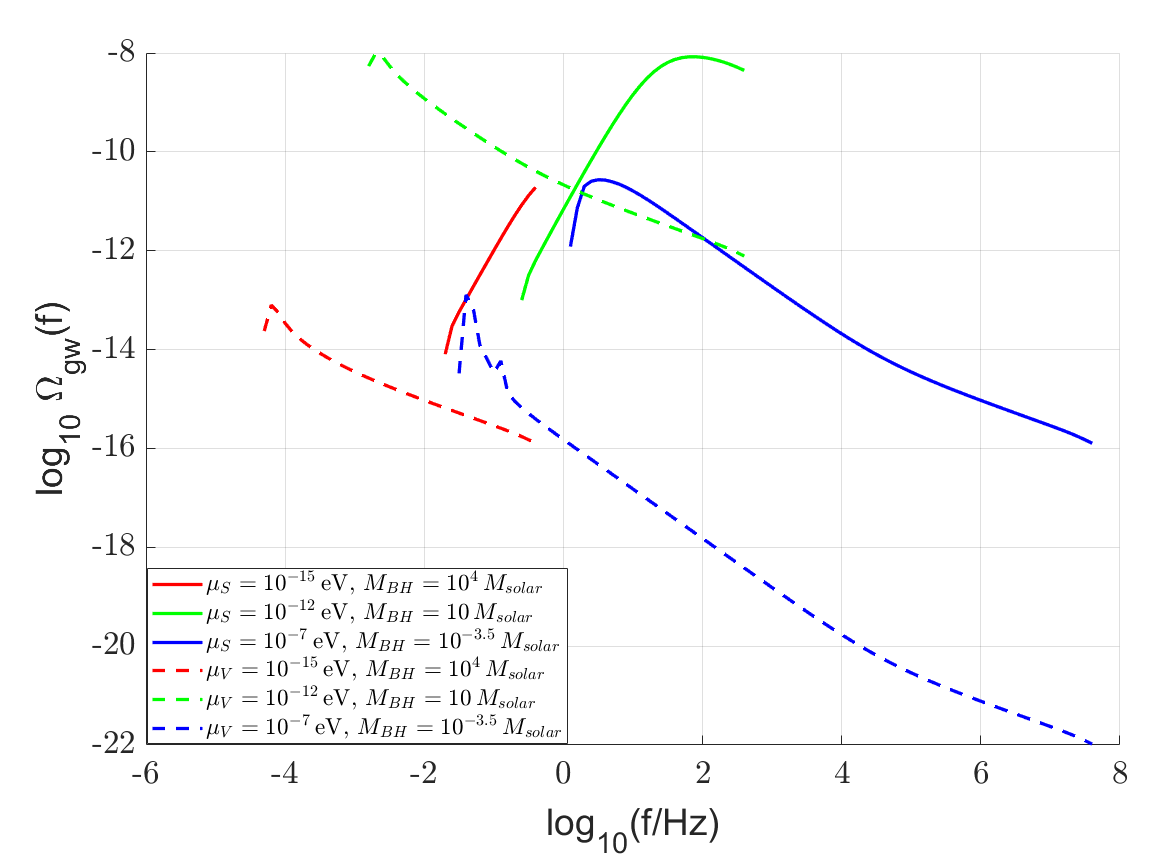
Figure 1: Samples of SGWB spectrums generated by PGA-0 (solid) and PGA-1 (dotted) in the short MD era scenario.

We can describe the above two competing effects more precisely, in terms of the characteristic cloud consumption time $\tau_{\rm GW}$. For the low frequency $f/\mu\ll\sqrt{\tau_{\rm GW}/\tilde{\tau}}$ emitted at $t(f)\ll\tau_{\rm GW}$, the energy of the cloud remains nearly constant, thus we have the rising spectrum $\Omega(f)\propto f^{3}$; it is a power law widely present in SGWB signals due to the pure redshift. On the contrary, for the high frequency $f/\mu\gg\sqrt{\tau_{\rm GW}/\tilde{\tau}}$ produced at $t(f)\gg\tau_{\rm GW}$, the effect of the cloud decay becomes more important than the redshift, so we have the falling spectrum $\Omega(f)\propto f^{-1}$, which is the characteristic power law specific to the SGWB from PGAs. More precisely, by solving $\frac{d\Omega_{\rm GW}(f)}{df}=0$, we find that the trend in the GW spectrum undergoes a transition at $f_{\rm peak}/\mu=\sqrt{3\tau_{\rm GW}/\tilde{\tau}}$ (i.e. $t(f_{\rm peak})=3\tau_{\rm GW}$), which is consistent with our physical expectations. In brief, the spectrum could be estimated by

$$\Omega_{\rm GW}\propto\begin{cases}f^{3}&\quad t_{0}<t(f)\lesssim 3\tau_{\rm GW}\\ f_{\rm peak}^{4}f^{-1}&\quad 3\tau_{\rm GW}\lesssim t(f)<t_{\rm eq}.\end{cases}$$ (3.34)

To our knowledge, this new spectrum is obtained for the first time, and it is distinguished from other SGWB signals. Although the approximate spectrum is only suitable in GWs from the RD era, it’s sufficient for a qualitative analysis of the complete spectrum, as shown in Fig. 1 and Fig. 2 .

Note that $\tau_{\rm GW}$, with a high power of $\mu$ and $M_{\rm BH}$, is a key parameter in the SGWB spectrum because it directly relates to the location of the peak frequency (very different from the original value $\mu/2$). The expressions of $\tau_{\rm GW}$ differ significantly in the scalar and vector cloud, leading to different spectrums. To manifest the difference, we give a few examples in Fig. 1. The solid lines represent the SGWB generated by PGA-0 in the short MD era scenario, the dotted lines are the SGWB generated by the PGA-1. It’s easy to find the $f^{\rm peak}$ of PGA-1 is significantly smaller compared to PGA-0 with the same $M_{\rm BH}$ and $\mu$. The solid red line has no $f^{\rm peak}$ because the corresponding $\tau_{\rm GW}$ is larger than the age of the universe.

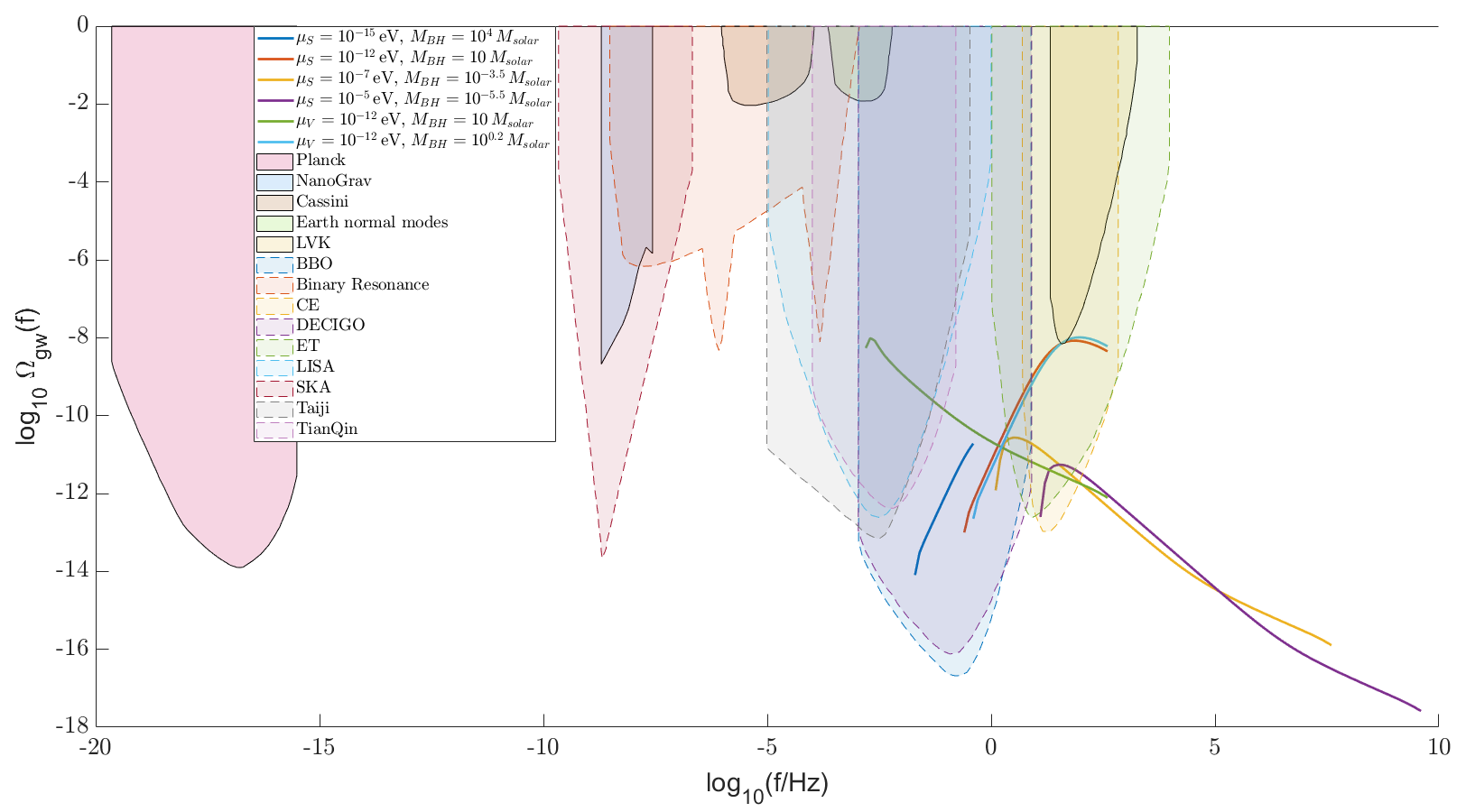
Figure 2: Constraints on SGWBs from existing GW detectors (shaded areas with thin solid bound lines), sensitivities of future detectors (shaded areas with thin dashed bound lines), and the SGWBs from the PGAs in the short MD era scenario (thick solid curves).

3.4 Results of SGWB from PGA: Constraints & Prospects

First of all, PBHs face a bunch of constraints, depending on the PBH mass, and they are comprehensively summarized in Ref. [28]. We assume that the dressed bosonic clouds do not affect these constraints, and explore PGAs in the allowed $(M_{\rm BH},f_{\rm PBH})$ plane. Our interest is the SGWB signal from PGAs, and in this part we demonstrate the current constraints and explore its prospects at the future detectors. Despite of the overall similarity, we discuss the spin-0 and spin-1 cases separately.

3.4.1 PGAs with a Scalar Cloud

Let us first investigate the typical PGAs that can produce observational SGWBs in the monochromatic mass scenario. For demonstration, we consider the cores produced in the short MD era studied previously, taking $I=1$. The PGAs in the universe can be characterized by three parameters $(\mu_{S},M_{\rm BH},f_{\rm PBH})$. Then, for each $(\mu_{S},M_{\rm BH})$ parameter point, we input different $f_{\rm PBH}$ values and calculate the GW spectrum from the corresponding PGAs. An upper bound $f^{\rm max}_{\rm PBH}(M_{\rm BH})$ is obtained by the requirement that the corresponding critical spectrum does not passes through any one of the shaded areas with thin solid boundary lines shown in Fig. 2. These exclusions are derived from various available experiments that are sensitive to SGWBs, including the Planck’s CMB temperature and polarization spectra [74, 75], NanoGrav’s approximate upper limit [76, 77], Cassini satellite Doppler tracking [78], Earth’s normal modes monitoring [79], and Advanced LIGO’s and Advanced Virgo’s O3 run combined with limits from earlier O1 and O2 runs (LVK) [80]. However, it is not difficult to observe that the constraints on the abundance of PBHs are entirely due to the contribution from LVK, as shown in Fig. 2.

Actually, in some PBH mass region, a proper cloud may boost the discovering of these PBHs via the GW signal. To show this, we add some plots in Fig. 3 where the existing strongest constraints are shaded in gray. It is seen that for $M_{\rm BH}\sim{\cal O}(1-100)~{}M_{\odot}$ subject to existing relatively weak constraints, the SGWB signal is already able to yield stronger constraints provided the scalar clouds with $\mu_{S}\sim{\cal O}(10^{-11}-10^{-13})~{}{\rm eV}$, which gives rise to GW spectras similar to the orange-red curve in Fig. 2; The constraints it provides even have several orders of magnitude enhancements.

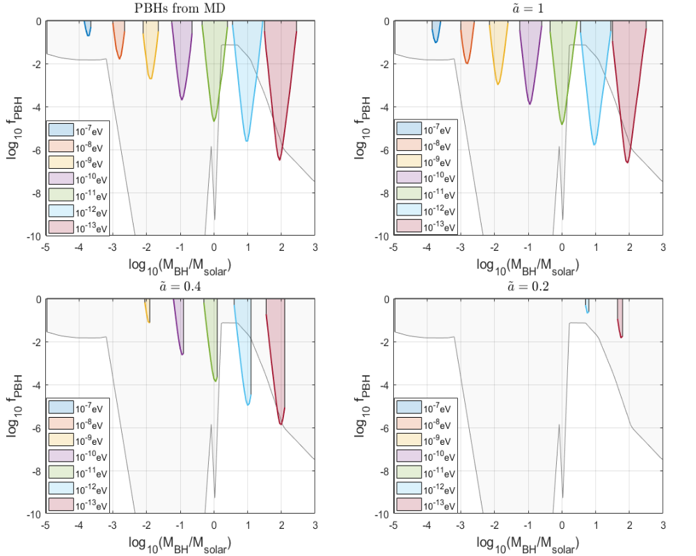
Figure 3: New constraint on PBHs by virtue of the SGWB signals from PGA-0 with several chosen $\mu_{S}$. The gray shaded areas denote the existing constraints.

To reveal the dependence of the spin, which is the peculiar feature of the PBHs that we are using and thus furnishes a way to distinguish the different origins of PBHs, we also scan the constraints on the $(\mu_{S},M_{\rm BH})$ plane by choosing three values of fixed $\tilde{a}$: 1, 0.4 and 0.2. The results are displayed in Fig. 4, where the narrow green/blue shaded bands can be excluded. The area of the excluded band shrinks as $\tilde{a}$ decreases, and in fact, we find that for $\tilde{a}=0.1$, there are no constraints at all.

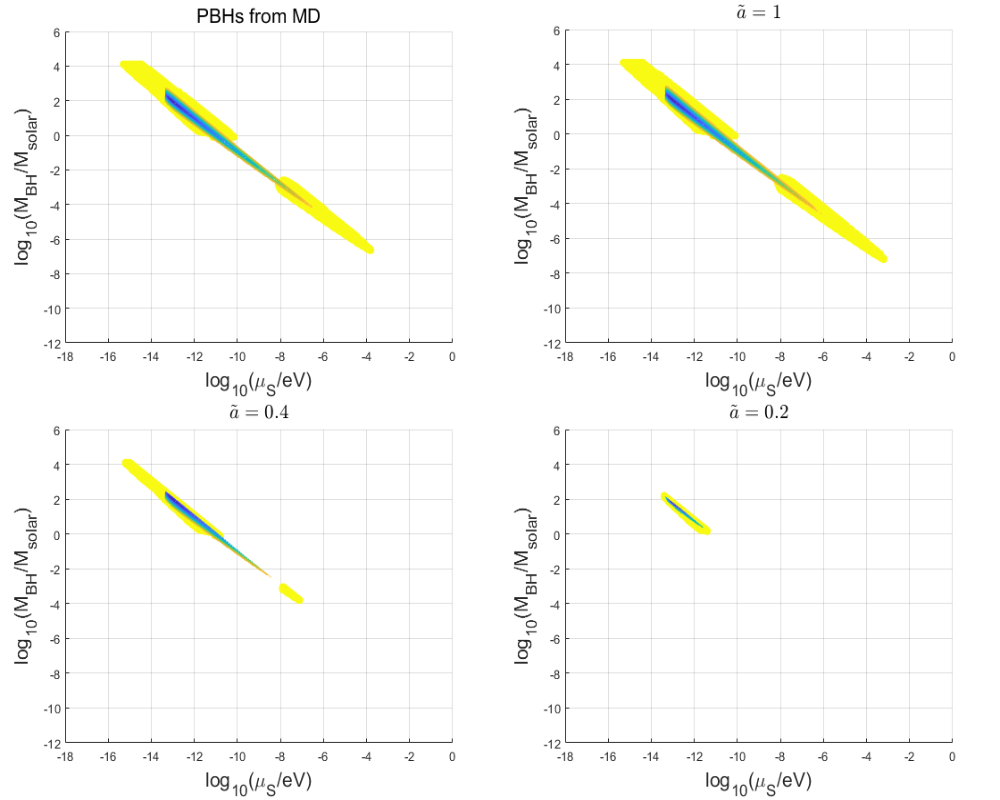
Figure 4: Constraints (blue and green bands) and prospects (yellow bands) of PGA-0, taking different spins $\tilde{a}$.

It is worth noting that, although changing the value of $\tilde{a}$ alters the strength of the corresponding constraints, for a given $\mu_{S}$, the mass central value of the PBHs constrained is essentially fixed (as shown in Fig. 3). This is not difficult to understand, as the primary effect of $\tilde{a}$ is on the magnitude of $\Omega_{\rm GW}$ through the saturation energy of the cloud $M_{C}^{\rm max}$, rather than its shape. We emphasize this because we will compare the mass central value of the PBHs constrained in the case of PGA-1.

The future GW detectors in different frequency bands are about to substantially enhance the current sensitivities, and thus it is of interest to see the prospects of various PGAs at these future detectors. This analysis includes considerations of the sensitivities of various future GW detectors, such as the Square Kilometre Array (SKA) [81], binary resonance searches [82, 83], Laser Interferometer Space Antenna (LISA) [84], Taiji [85], TianQin[86], Deci-hertz Interferometer Gravitational wave Observatory (DECIGO) [87], Big Bang Observer (BBO) [88], Einstein Telescope (ET) [89], and Cosmic Explorer (CE) [90]. Their expected sensitivity curves are shown by the shaded areas with thin dashed bound lines in Fig. 2, where, we exhibit a group of promising $(M_{\rm BH},\mu_{S})$ samples in the short MD era scenario, $(\mu_{S},M_{\rm BH})=(10^{-15}{\rm eV},10^{4}M_{\odot}),~{}(10^{-12}{\rm eV},10M_{\odot}),~{}(10^{-7}{\rm eV},10^{-3.5}M_{\odot}),~{}(10^{-5}{\rm eV},10^{-5.5}M_{\odot})$, taking the upper limit of $f_{\rm PBH}(M_{\rm BH})$. One can see that, the infrared part and the peak frequency of a given spectrum may be probed by different detectors which have the best sensitivity at quite different bands.

It is of importance to make a more overall estimation on the GW prospects of PGAs. To that end, we consider the short MD era scenario and three values of fixed $\tilde{a}$: 1, 0.4, and 0.2. The expected detectable parameter regions by these future detectors are shown in Fig. 4. The yellow regions in the figure indicate the parameter spaces where the SGWB are expected to be detectable. In the mass window $M_{\rm BH}=10^{-3}M_{\odot}\sim 1M_{\odot}$, no observable GWs are expected, due to the existing strict constraints on the abundance of PBHs in this mass range. If future observations do not detect signals in the yellow parameter spaces, it would imply even more stringent constraints on the abundance of PBHs in those regions.

3.4.2 PGAs with a Vector Cloud

Let us move to the analysis of PGA-1. The results are found to be quite similar to PGA-0, except that the vector boson spin brings a mild difference. We consider the short MD era scenario and three values of fixed $\tilde{a}$: 1, 0.1, and 0.04 for our analysis. We primarily discuss several remarkable differences between the detection of PGA-0 and PGA-1.

• Firstly, it is observed that for the same boson mass $\mu_{V}=\mu_{S}$, the central value of the currently constrained PGA-1 mass shifts approximately $1~{}M_{\odot}$ to the left, compared to PGA-0, as illustrated in Fig. 3 and Fig. 5. To see how it happened, let us consider the sample $(\mu_{S}=\mu_{V}=10^{-12}~{}\rm eV,M_{BH}=10~{}M_{\odot})$. For PGA-0, the resulting SGWB near $f_{\rm peak}$ is constrained by LVK, shown in Fig. 2. However, for PGA-1, the resulting amplitude $\Omega_{\rm GW}(f)$ is significantly lower than the detection sensitivity of LVK due to the lower $f_{\rm peak}$ compared to PGA-0. So, for $\mu_{V}=\mu_{S}$, only the lighter PGA-1 (i.e., smaller $\alpha$) can achieve a relatively higher $\tau_{\rm GW}$, allowing the SGWB to reach the sensitivity of LVK, as shown by the line $\mu_{V}=10^{-12}~{}\rm eV$ and $M_{\rm BH}=10^{0.2}~{}M_{\odot}$ in Fig. 2.

  

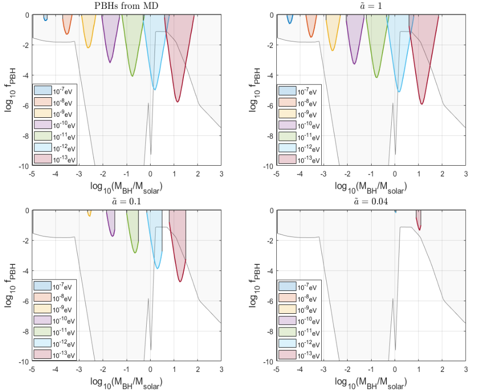
  Figure 5: New constraints on PBHs by virtue of the SGWB signals from PGA-1 with several chosen $\mu_{V}$. The gray shaded areas denote the existing constraints.

• Secondly, PGA-1 still have a significant parameter space constrained by the SGWB for its core dimensionless spin values as low as $\sim\mathcal{O}(0.01)$, which is obviously lower than the threshold for PGA-0 discussed earlier, $\sim 0.1$ (compare Fig. 3 with Fig. 5). This is because the superradiance condition in Eq. (3.11) selects certain PGAs with $\tilde{a}>\tilde{a}_{s}\equiv\frac{4\alpha}{4\alpha^{2}+1}$ and $\alpha<0.5$, with the former setting the lower threshold on the feasible $\tilde{a}$. Let’s consider the example where the mass of the boson is $\mu_{S}=\mu_{V}=10^{-13}\text{eV}$. For PGA-0, the main constraint is at $M_{\rm BH}\sim 10^{2}M_{\odot}$, corresponding to $\tilde{a}_{s}\simeq 0.3$. However, for PGA-1, the main constraint is at $M_{\rm BH}\sim 10M_{\odot}$ (as discussed in the first point), with the corresponding $\tilde{a}_{s}$ being about an order of magnitude smaller, $\sim 0.03$. It’s obvious that the the lower threshold for PGA-1 is smaller compared to PGA-0.

• Thirdly, as shown in Fig. 4 and Fig. 6, the PGA-1 located in the parameter space $(\mu_{V},M_{\rm BH})$ has a significantly wider detectable area, compared to PGA-0 in the parameter space $(\mu_{S},M_{\rm BH})$ (taking the same spin distribution). This is due to the more effective GW emission rate of the PGA-1 than PGA-0 for the same $\alpha$, which enhances the detectablity of PGA-1 through a lower peak frequency. It makes the SGWB enter the sensitivities of the powerful detectors such as LISA, Taiji, and TianQin, as shown by the spectrum for $\mu_{V}=10^{-12}~{}\rm eV$ and $M_{\rm BH}=10~{}M_{\odot}$ in Fig. 2.

  

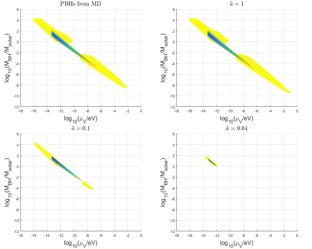
  Figure 6: Constraints (blue and green bands) and prospects (yellow bands) of PGA-1, taking different spins $\tilde{a}$.

Note that the fundamental difference between the two kinds of PGAs lies in the different $f_{\rm peak}$ caused by $\tau_{\rm GW}$.

4 Discussions and Conclusions

Gravitational atoms have been an interesting interdisciplinary field between astronomy and particle physics, and inspire a lot of studies. But if the cores of GAs are PBHs, then cosmology joins. This scenario has not been carefully studied yet, probably owing to the lacking evidence of PBHs, in particular PBHs with a large spin. However, observations really call for primordial origins of black holes and moreover PBH relics are well expected in the early universe.

In this article, we aim at investigating the general features of GWs from PGAs. To make the discussion more concrete, we consider a representative monochromatic mass scenario where PBHs form during a short MD era. In this scenario, the PBHs acquire a large spin at formation and do not lose it through accretion. We compute the GW signals generated by the boson clouds and, through approximate analysis, we find that PGAs in the universe leave an imprint as a SGWB. This spectrum is characterized by a rising $\propto f^{3}$ followed by a falling $\propto f^{-1}$, distinguishing it from other sources of GW signals. Furthermore, we provide constraints of the abundance of PGAs. We find that, compared to bare PBHs with $M_{\rm BH}\sim\mathcal{O}(10)M_{\odot}$, PGA-0 with $\mu_{S}\sim\mathcal{O}(10^{-13})\text{ eV}$ and PGA-1 with $\mu_{V}\sim\mathcal{O}(10^{-12})\text{ eV}$ are imposed stronger constraints. Additionally, by considering future GW detectors such as LISA, Taiji, and TianQin, we identify a narrow and elongated parameter space. In the near future, we will know whether these PGAs are detected or further constrained.

This is a tentative study and many things need to be further cleared or improved. The most urgent one, we think is the effect of non-rotating matter accretion around the PBHs formed during the MD era. Specific simulation (based on the classical field behaving as matter) indicates that it may reduce the initially large dimensionless spin. Although there is no comprehensive research about the PBH spin evolution during the MD era, we could estimate the effect of accretion. In Ref. [35], the secondary infall model was used to consider the spherically symmetric accretion of non-spinning PBHs, where the PBH mass grows as $M_{\rm BH}\propto a\propto t^{2/3}$. Assuming that the rotating PBH exhibit a similar accretion behavior, then $\tilde{a}\propto a^{-1}$ according to the conservation of total angular momentum. Clearly, even if the initial dimensionless spin is at the maximum value of 1, it will be reduced to approximately 0.1 after two e-folds.

In this paper, we focus on a short MD era to prevent spin reduction. However, it is worthing note that our results are remain significant when extended to a longer MD era. The constraints we place on PBHs and the prospects we discuss are applicable to those cores formed near the reheating period ($M_{\rm BH}\simeq M_{\rm max}$). These black holes, which might carry vital clues about the early universe, have the potential to help us understand the origins of cosmic history.

Moreover, the SGWB energy density frequency spectrum $\Omega_{\rm GW}(f)$ is very sensitive to the core mass, as $\frac{d\tilde{E}}{dt}\propto M_{\text{BH}}^{14}$ for PGA-0 and $\frac{d\tilde{E}}{dt}\propto M_{\text{BH}}^{10}$ for PGA-1 as shown in Eq. (3.1.2) and Eq. (3.25). The fact implies that the evolution of core mass could play a crucial role, including their late accretion and cosmic evolution. However, the energy extraction from cores by superradiant clouds does not have a significant impact. This is because the superradiance process affects the black hole’s mass by at most $10.78\%$ [66], which does not change the order of magnitude of $\Omega_{\rm GW}(f)$.

Appendix A PBHs Formed during a MD Epoch

A.1 The PBH Mass

Consider a perturbation with scale $k$, its density contrast $\delta(k)\equiv(\rho-\bar{\rho})/\bar{\rho}$ describes the fluctuation relative to the background. Its behavior after entering the Hubble horizon is quite interesting, because causality becomes established. The time of horizon crossing is $t_{H}(k)$, which is determined by the equality between the physical length $a(t_{H}(k))/k$ and Hubble horizon length $1/H(t_{H}(k))$, thus $t_{H}(k)=\frac{8a_{m}}{3k^{3}}$ (the subscript $H$ emphasizes that this quantity is defined at the time of horizon crossing, and $a_{m}$ is a constant). Primordial fluctuations are random and generally follow a Gaussian distribution. At $t=t_{H}(k)$, the probability distribution of the density contrast is

$$P(\delta_{H})=\frac{1}{\sqrt{2\pi}\sigma_{H}}\exp\left(-\frac{\delta_{H}^{2}}{2\sigma_{H}(k)^{2}}\right),$$ (A.1)

where $\sigma_{H}$ is much smaller than 1 in general, thus the majority of perturbations satisfies $\delta_{H}\sim\sigma_{H}\ll 1$. After the perturbation crosses the Hubble horizon, it continues to expand following the Hubble flow, but the expansion gradually slows down due to the gravity. Consequently, the density contrast increases, a process that can be described using the results of linear perturbation theory as $\delta=\delta_{H}a(t)/a(t_{H})\propto t^{2/3}$. When the perturbation has expanded to its maximum size (at $t=t_{d}$), it decouples from the background, and then the perturbation collapses. Since $\delta\sim 1$ typically occurs at $t=t_{d}$ (which implies $t_{d}(k)\sim t_{H}(k)\delta_{H}(k)^{-3/2}=\frac{8a_{m}}{3k^{3}}\delta_{H}(k)^{-3/2}$), this collapse can no longer be described by the linear theory. The collapse completes at $t=t_{c}$, with $t_{c}$ generally being of the same order as $t_{d}$ .

The probability $\beta(k)$ for collapsing to a PBH is discussed in Appendix A.2. It actually gives the corresponding energy fraction of the formed PBH if the resulting PBH mass $M_{\rm BH}$ is the Hubble mass at horizon crossing $M_{H}(k)=\frac{M_{\rm PL}^{2}}{2H(t_{H}(k))}\propto t_{H}(k)$. Therefore, the PBH born later has a larger mass.

For the perturbation with $t_{c}(k)>t_{\rm end}$, the universe enters the RD era before the collapse completes. This significantly reduces the probability of PBH formation. Therefore, we only consider the perturbations satisfying

$$t_{c}(k)\sim t_{d}(k)\sim t_{H}(k)\delta_{H}(k)^{-3/2}\in(t_{\rm ini},t_{\rm end}).$$ (A.2)

The PBH mass spectrum starts from $M_{\rm min}=M_{H}(t_{\rm ini})$, since the scale $k_{\rm ini}$ entering horizon at $t_{\rm ini}$ is supposed to have sufficient time to evolve and collapse in the MD era. The PBH mass spectrum ends at $M_{\rm max}=M_{H}(t_{\rm max})$, which originate from perturbations with $k=k_{\text{max}}$, defined by $t_{c}(k_{\rm max})=t_{\rm end}$. Then, the corresponding PBH mass is given by

$$M_{\text{max}}=M_{H}(t_{\text{end}})\frac{t_{H}(k_{\rm max})}{t_{\text{end}}}\simeq M_{H}(t_{\text{end}})\delta^{3/2}_{H}(k_{\text{max}})\simeq M_{H}(t_{\text{end}})\sigma^{3/2}_{\text{max}},$$ (A.3)

where $\sigma_{\rm max}\equiv\sigma_{H}(k_{\rm max})$.

A.2 The Production Rate and Spin Distribution

Harada et al. in Ref. [44] considered that a uniformly distributed spherically symmetric region that, upon entering the horizon, undergoes anisotropic collapse, as shown in

$$\begin{cases}r_{1}=(a-\alpha b)q_{1}\\ r_{2}=(a-\beta b)q_{2}~{},\\ r_{3}=(a-\gamma b)q_{3}\end{cases}$$

where $\alpha,\beta,\gamma$ are constant satisfying $\alpha>\beta>\gamma$ and $\delta_{H}=\alpha+\beta+\gamma>0$ . The probability distribution function for them is given by Doroshkevich [44] as

$$w(\alpha,\beta,\gamma)=-\frac{27}{8\sqrt{5}\pi\sigma_{3}^{6}}\exp{\left[-\frac{3}{5\sigma_{3}^{2}}(\alpha^{2}+\beta^{2}+\gamma^{2})-\frac{1}{2}(\alpha\beta+\beta\gamma+\gamma\alpha)\right]}(\alpha-\beta)(\beta-\gamma)(\gamma-\alpha).$$ (A.4)

It is consistent with Eq. (A.1) and $\sigma_{H}=\sqrt{5}\sigma_{3}$. Due to the anisotropy of collapse, this overdense region forms a pancake. According to the hoop conjecture, if it satisfies $h(\alpha,\beta,\gamma)\lesssim 1$, it eventually collapses into a black hole, where

$$h(\alpha,\beta,\gamma)\equiv\frac{2}{\pi}\frac{\alpha-\gamma}{\alpha^{2}}E\left(\sqrt{1-\left(\frac{\alpha-\beta}{\alpha-\gamma}\right)^{2}}\right),$$ (A.5)

and $E(e)$ is the complete elliptic integral of the second kind. The production rate $\beta_{\text{ani}}$ is given by

$$\beta_{\text{ani}}=\int^{\infty}_{0}d\alpha\int^{\alpha}_{-\infty}d\beta\int^{\beta}_{-\infty}d\gamma\theta[\delta_{H}(1-h(\alpha,\beta,\gamma)]\omega(\alpha,\beta,\gamma),$$ (A.6)

which is best fit by $\beta_{\text{ani}}=0.056\sigma_{H}^{5}$ for small $\sigma_{H}$.

Subsequently, the effect of spin on black hole collapse was considered in Ref. [34]. According to their assumptions, the spin of the product after the collapse of the overdense region ultimately receives two contributions

$$\tilde{a}=\tilde{a}_{(1)}+\tilde{a}_{(2)}\approx\text{max}(\tilde{a}_{(1)},\tilde{a}_{(2)})~{},~{}\,$$ (A.7)

where

$$\tilde{a}_{(1)}=\frac{2}{5}\sqrt{\frac{3}{5}}q(\delta_{H})^{-1/2}\ \text{and}\ \tilde{a}_{(2)}=\frac{2}{5}I(\delta_{H})^{-3/2}.$$ (A.8)

$q$ is a dimensionless constant describing the initial shape of the perturbation ($q=0$ refers to a sphere), and its distribution is unknown to our knowledge, which brings theoretical uncertainty to the quantitative study of the PBH spin distribution. $I$ is another dimensionless constant related to the perturbation power spectrum. According to the calculations of several power spectrum in [92], it’s can be assumed that $I\sim 1$. In this paper, we always take $I=1$. Black holes must satisfy $\tilde{a}<1$, therefore, they argued that the pancake satisfying $\tilde{a}<1$ will eventually form a black hole, which imposes a threshold for PBH formation, $\delta_{\text{th}}=\text{max}(\delta_{\text{th}}^{(1)},\delta_{\text{th}}^{(1)})\equiv\text{max}(\frac{12}{125}q^{2},(\frac{2}{5}I\sigma_{H})^{\frac{2}{3}})$ from Eq. (A.8) by setting $\tilde{a}=1$. It is seen that, $\delta_{\text{th}}=\delta_{\text{th}}^{(1)}$ when $q>q_{c}\equiv\sqrt{\frac{2}{3}}(\frac{5}{2})^{7/6}I^{1/3}\sigma_{H}^{1/3}\sim\sigma_{H}^{1/3}$; $\delta_{\text{th}}=\delta_{\text{th}}^{(2)}$ when $q<q_{c}$. Combining the effects of spin and anisotropic collapse on the PBH formation, the probability for a perturbation collapsing to a PBH can be calculated by

$$\beta_{\text{ani+spin}}\simeq\int^{\infty}_{0}d\alpha\int^{\alpha}_{-\infty}d\beta\int^{\beta}_{-\infty}d\gamma\theta[\delta_{H}(\alpha,\beta,\gamma)-\delta_{th}]\theta[\delta_{H}(1-h(\alpha,\beta,\gamma)]\omega(\alpha,\beta,\gamma)~{}.~{}\,$$ (A.9)

The numerical results are shown in Figure 5 in Ref. [34], and the semi-analytical results are provided below. For $q>q_{c}(\delta_{th}=\delta_{th}^{(1)})$, we have

$$\beta_{\text{(1)ani+spin}}\simeq\begin{cases}3.244\times 10^{-14}\cfrac{q^{18}}{\sigma_{H}^{4}}\exp\left[-0.004608\cfrac{q^{4}}{\sigma_{H}^{2}}\right]&\quad(\sigma_{H}\lesssim 0.04)\\ 0.056\sigma_{H}^{5}&\quad(0.04\lesssim\sigma_{H}\lesssim 0.2)~{}.{}\end{cases}$$ (A.10)

While for $q<q_{c}(\delta_{th}=\delta_{th}^{(2)})$, we have

$$\beta_{\text{(2)ani+spin}}\simeq\begin{cases}1.921\times 10^{-7}I^{6}\sigma_{H}^{2}\exp\left[-0.1474\cfrac{I^{4/3}}{\sigma_{H}^{2/3}}\right]&\quad(\sigma_{H}\lesssim 0.005)\\ 0.056\sigma_{H}^{5}&\quad(0.005\lesssim\sigma_{H}\lesssim 0.2)~{}.\end{cases}$$ (A.11)

According to Eq. (2.8), we can estimate $\sigma_{H}$. Noting that we are only concerned with the upper limit of $f_{\text{PBH}}$, which lies between $10^{-10}$ and 1, as shown in Fig. 3 and Fig. 5, thus we estimate $0.002\lesssim\sigma_{H}\lesssim 0.08$. Of course, when $10^{-2.5}M_{\odot}\lesssim M_{\rm BH}\lesssim 10^{-0.5}M_{\odot}$, $f_{\text{PBH}}$ can be much less than $10^{-10}$. However, we find that this range does not yield a detectable SGWB, and thus it does not affect our discussions.

For $0.002\lesssim\sigma_{H}\lesssim 0.04$, it is not difficult to observe $\beta_{\text{(2)ani+spin}}\gg\beta_{\text{(1)ani+spin}}$, which implies that the majority of PBHs originate from overdense regions satisfying $q<q_{c}$. Considering statistical averaging, the production rate of PBHs is approximately equal to $f(q_{c})\beta_{\text{ani+spin(2)}}\simeq f(q_{c})\beta_{\text{ani}}$ (with a difference of approximately an ${\cal O}(1)$ factor when $0.002\lesssim\sigma_{H}\lesssim 0.005$). The factor $f(q_{c})$ represents the proportion of $q<q_{c}$ and depends on the initial distribution of $q$, which is unknown to our knowledge. For $0.04\lesssim\sigma_{H}\lesssim 0.08$, $\beta_{\text{ani+spin}}=\beta_{\text{ani}}$, and the production rates for $q<q_{c}$ and $q>q_{c}$ are equal. Note that the range of $q_{c}$ we are interested in satisfies $0.3\lesssim q_{c}\lesssim 1$ by estimation. As a preliminary exploration, we assume that the vast majority of overdense regions satisfy $q<q_{c}$, thus $f(q_{c})=1$. Consequently, in the scenario we consider, $\beta_{\text{ani+spin}}=\beta_{\text{ani}}$, indicating that PBH formation is independent of spin.

In Ref. [45], the PBH production probability of spherically symmetric but inhomogeneous distributed overdense regions is calculated, being fit by $\beta_{\text{inhom}}\simeq 3.6979\sigma_{H}^{3/2}/\Sigma$, where $\Sigma\sim{\cal O}(1)$. This fits well when $\sigma_{H}\lesssim 0.05$, and there is a difference of approximately an ${\cal O}(1)$ factor when $0.05\lesssim\sigma_{H}\lesssim 0.08$. Therefore, $\beta_{\text{inhom}}\simeq 3.6979\sigma_{H}^{3/2}$. To combine the effects of the inhomogeneity and anisotropy on the PBH formation (the spin has no effect), we further assume that all overdense regions are very close to sphericity, so that $q\ll q_{c}\sim 1$. In this case, the prodution rate is expected as the simple multiplication of $\beta_{\text{inhom}}$ and $\beta_{\text{ani}}$,

$$\beta_{\text{ani+spin+inhom}}=\beta_{\text{inhom}}\times\beta_{\text{ani}}\simeq 0.2055\sigma_{H}^{13/2}.$$ (A.12)

At the same time, under the assumption that $q\ll q_{c}$, for the majority of PBHs, $\tilde{a}_{(2)}>\tilde{a}_{(1)}$ (see Fig. 2 in Ref. [34]). Thus, $\tilde{a}\simeq\tilde{a}_{(2)}$. According to the results in Ref. [34], we can infer that the spin distribution of PBHs at formation is

$$P_{2}(\tilde{a})\propto\frac{1}{\tilde{a}^{5/3}}\exp\left(-\frac{1}{2\sigma_{H}^{2/3}}\left(\frac{2}{5}I\right)^{4/3}\frac{1}{\tilde{a}^{4/3}}\right)~{}.$$ (A.13)

We have plotted $P_{2}(\tilde{a})$ for $\sigma_{H}=0.08$, $\sigma_{H}=0.01$ and $\sigma_{H}=0.002$, as shown in Fig. 7. It’s evident that the smaller the $\sigma_{H}$, the more concentrated the initial spins of PBHs are around $\tilde{a}=1$. This is because a smaller perturbation require more time to reach the maximum expansion, giving the dimensionless spin ample time to grow (see Ref. [34] for details).

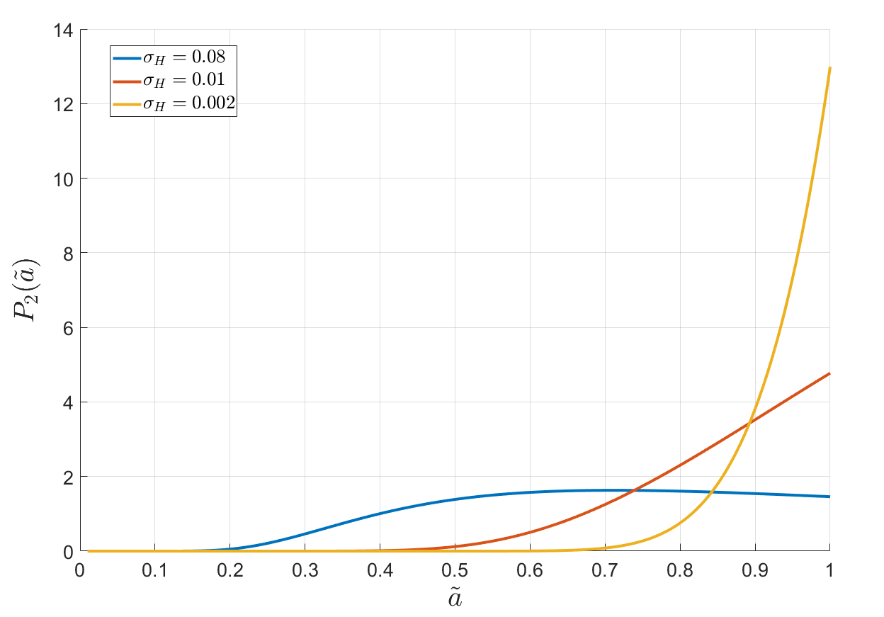
Figure 7: The spin distribution of PBHs. The lines with different color denote the different $\sigma_{H}$.

References

- [1] Richard Brito, Vitor Cardoso, and Paolo Pani. Superradiance: New Frontiers in Black Hole Physics. Springer International Publishing, 2020.
- [2] William H Press and Saul A Teukolsky. Floating orbits, superradiant scattering and the black-hole bomb. Nature, 238(5361):211–212, 1972.
- [3] Vitor Cardoso, Oscar JC Dias, José PS Lemos, and Shijun Yoshida. Black-hole bomb and superradiant instabilities. Physical Review D, 70(4):044039, 2004.
- [4] Th Damour, N Deruelle, and R Ruffini. On quantum resonances in stationary geometries. Lettere al Nuovo Cimento (1971-1985), 15:257–262, 1976.
- [5] Theodoros JM Zouros and Douglas M Eardley. Instabilities of massive scalar perturbations of a rotating black hole. Annals of physics, 118(1):139–155, 1979.
- [6] Steven L. Detweiler. KLEIN-GORDON EQUATION AND ROTATING BLACK HOLES. Phys. Rev. D, 22:2323–2326, 1980.
- [7] Hironobu Furuhashi and Yasusada Nambu. Instability of massive scalar fields in kerr-newman spacetime. Progress of theoretical physics, 112(6):983–995, 2004.
- [8] Vitor Cardoso and Shijun Yoshida. Superradiant instabilities of rotating black branes and strings. Journal of High Energy Physics, 2005(07):009, 2005.
- [9] Sam R Dolan. Instability of the massive klein-gordon field on the kerr spacetime. Physical Review D, 76(8):084001, 2007.
- [10] João G Rosa. The extremal black hole bomb. Journal of High Energy Physics, 2010(6):1–20, 2010.
- [11] Sam R Dolan. Superradiant instabilities of rotating black holes in the time domain. Physical Review D, 87(12):124026, 2013.
- [12] William E East and Frans Pretorius. Superradiant instability and backreaction of massive vector fields around kerr black holes. Physical review letters, 119(4):041101, 2017.
- [13] William E East. Superradiant instability of massive vector fields around spinning black holes in the relativistic regime. Physical Review D, 96(2):024004, 2017.
- [14] Sam R Dolan. Instability of the proca field on kerr spacetime. Physical Review D, 98(10):104006, 2018.
- [15] Shou-Shan Bao, Qi-Xuan Xu, and Hong Zhang. Improved analytic solution of black hole superradiance. Physical Review D, 106(6):064016, 2022.
- [16] Richard Brito and Paolo Pani. Black-hole superradiance: Searching for ultralight bosons with gravitational waves. Handbook of Gravitational Wave Astronomy, pages 1–33, 2020.
- [17] YB Zel’dovich. I.. d. novikov, azh 43 (1966) 758; yb zel’dovich and id novikov. Sov. Astron. AJ, 10:602, 1967.
- [18] Stephen Hawking. Gravitationally collapsed objects of very low mass. Monthly Notices of the Royal Astronomical Society, 152(1):75–78, 1971.
- [19] Bernard J Carr and Stephen W Hawking. Black holes in the early universe. Monthly Notices of the Royal Astronomical Society, 168(2):399–415, 1974.
- [20] George F Chapline. Cosmological effects of primordial black holes. Nature, 253(5489):251–252, 1975.
- [21] Bernard Carr and Florian Kühnel. Primordial black holes as dark matter: recent developments. Annual Review of Nuclear and Particle Science, 70:355–394, 2020.
- [22] Anne M Green and Bradley J Kavanagh. Primordial black holes as a dark matter candidate. Journal of Physics G: Nuclear and Particle Physics, 48(4):043001, 2021.
- [23] Benjamin P Abbott, Richard Abbott, TDe Abbott, MR Abernathy, Fausto Acernese, Kendall Ackley, Carl Adams, Thomas Adams, Paolo Addesso, RX Adhikari, et al. Observation of gravitational waves from a binary black hole merger. Physical review letters, 116(6):061102, 2016.
- [24] Simeon Bird, Ilias Cholis, Julian B Muñoz, Yacine Ali-Haïmoud, Marc Kamionkowski, Ely D Kovetz, Alvise Raccanelli, and Adam G Riess. Did ligo detect dark matter? Physical review letters, 116(20):201301, 2016.
- [25] Sebastien Clesse and Juan García-Bellido. The clustering of massive primordial black holes as dark matter: measuring their mass distribution with advanced ligo. Physics of the Dark Universe, 15:142–147, 2017.
- [26] Misao Sasaki, Teruaki Suyama, Takahiro Tanaka, and Shuichiro Yokoyama. Primordial black hole scenario for the gravitational-wave event gw150914. Physical review letters, 117(6):061101, 2016.
- [27] Bernard Carr, Sebastien Clesse, Juan Garcia-Bellido, Michael Hawkins, and Florian Kuhnel. Observational evidence for primordial black holes: A positivist perspective. arXiv preprint arXiv:2306.03903, 2023.
- [28] Bernard Carr, Kazunori Kohri, Yuuiti Sendouda, and Jun’ichi Yokoyama. Constraints on primordial black holes. Reports on Progress in Physics, 84(11):116902, 2021.
- [29] Tomohiro Harada, Chul-Moon Yoo, and Kazunori Kohri. Threshold of primordial black hole formation. Physical Review D, 88(8):084051, 2013.
- [30] Takeshi Chiba and Shuichiro Yokoyama. Spin distribution of primordial black holes. Progress of Theoretical and Experimental Physics, 2017(8):083E01, 2017.
- [31] Valerio De Luca, V Desjacques, G Franciolini, A Malhotra, and A Riotto. The initial spin probability distribution of primordial black holes. Journal of Cosmology and Astroparticle Physics, 2019(05):018, 2019.
- [32] Mehrdad Mirbabayi, Andrei Gruzinov, and Jorge Noreña. Spin of primordial black holes. Journal of Cosmology and Astroparticle Physics, 2020(03):017, 2020.
- [33] Yu. N. Eroshenko. Spin of primordial black holes in the model with collapsing domain walls. JCAP, 12(12):041, 2021.
- [34] Tomohiro Harada, Chul-Moon Yoo, Kazunori Kohri, and Ken-Ichi Nakao. Spins of primordial black holes formed in the matter-dominated phase of the universe. Physical Review D, 96(8):083517, 2017.
- [35] Valerio De Luca, Gabriele Franciolini, Alex Kehagias, Paolo Pani, and Antonio Riotto. Primordial black holes in matter-dominated eras: The role of accretion. Phys. Lett. B, 832:137265, 2022.
- [36] Eloy de Jong, Josu C Aurrekoetxea, and Eugene A Lim. Primordial black hole formation with full numerical relativity. Journal of Cosmology and Astroparticle Physics, 2022(03):029, 2022.
- [37] Enrico Barausse and Luciano Rezzolla. Predicting the direction of the final spin from the coalescence of two black holes. The Astrophysical Journal, 704(1):L40, 2009.
- [38] Paolo Pani and Abraham Loeb. Constraining primordial black-hole bombs through spectral distortions of the cosmic microwave background. arXiv preprint arXiv:1307.5176, 2013.
- [39] Paulo B Ferraz, Thomas W Kephart, and João G Rosa. Superradiant pion clouds around primordial black holes. Journal of Cosmology and Astroparticle Physics, 2022(07):026, 2022.
- [40] Nuno P Branco, Ricardo Z Ferreira, and João G Rosa. Superradiant axion clouds around asteroid-mass primordial black holes. Journal of Cosmology and Astroparticle Physics, 2023(04):003, 2023.
- [41] James B Dent, Bhaskar Dutta, and Tao Xu. Multi-messenger probes of asteroid mass primordial black holes: Superradiance spectroscopy, hawking radiation, and microlensing. arXiv preprint arXiv:2404.02956, 2024.
- [42] Indra Kumar Banerjee and Ujjal Kumar Dey. Gravitational wave probe of primordial black hole origin via superradiance. Journal of Cosmology and Astroparticle Physics, 2024(04):049, 2024.
- [43] V. De Luca, G. Franciolini, P. Pani, and A. Riotto. The evolution of primordial black holes and their final observable spins. JCAP, 04:052, 2020.
- [44] Tomohiro Harada, Chul-Moon Yoo, Kazunori Kohri, Ken-ichi Nakao, and Sanjay Jhingan. Primordial black hole formation in the matter-dominated phase of the universe. The Astrophysical Journal, 833(1):61, 2016.
- [45] Takafumi Kokubu, Koutarou Kyutoku, Kazunori Kohri, and Tomohiro Harada. Effect of inhomogeneity on primordial black hole formation in the matter dominated era. Physical Review D, 98(12):123024, 2018.
- [46] Tomohiro Harada, Kazunori Kohri, Misao Sasaki, Takahiro Terada, and Chul-Moon Yoo. Threshold of primordial black hole formation against velocity dispersion in matter-dominated era. Journal of Cosmology and Astroparticle Physics, 2023(02):038, 2023.
- [47] Sean M Carroll and Manoj Kaplinghat. Testing the friedmann equation: The expansion of the universe during big-bang nucleosynthesis. Physical Review D, 65(6):063507, 2002.
- [48] Dan Hooper and Huangyu Xiao. Dark matter is the new bbn. Physics of the Dark Universe, 42:101353, 2023.
- [49] M Yu Khlopov and AG Polnarev. Primordial black holes as a cosmological test of grand unification. Physics Letters B, 97(3-4):383–387, 1980.
- [50] AG Polnarev and M Yu Khlopov. Era of superheavy-particle dominance and big bang nucleosynthesis. Sov. Astron.(Engl. Transl.);(United States), 26(1), 1982.
- [51] Asher Berlin, Dan Hooper, and Gordan Krnjaic. Pev-scale dark matter as a thermal relic of a decoupled sector. Physics Letters B, 760:106–111, 2016.
- [52] Tommi Tenkanen and Ville Vaskonen. Reheating the standard model from a hidden sector. Physical Review D, 94(8):083516, 2016.
- [53] Rouzbeh Allahverdi and Jacek K Osiński. Early matter domination from long-lived particles in the visible sector. Physical Review D, 105(2):023502, 2022.
- [54] Anne M Green, Andrew R Liddle, and Antonio Riotto. Primordial black hole constraints in cosmologies with early matter domination. Physical Review D, 56(12):7559, 1997.
- [55] Gordon Kane, Kuver Sinha, and Scott Watson. Cosmological moduli and the post-inflationary universe: a critical review. International Journal of Modern Physics D, 24(08):1530022, 2015.
- [56] Andreas Albrecht, Paul J Steinhardt, Michael S Turner, and Frank Wilczek. Reheating an inflationary universe. Physical Review Letters, 48(20):1437, 1982.
- [57] Lev Kofman, Andrei Linde, and Alexei A Starobinsky. Reheating after inflation. Physical Review Letters, 73(24):3195, 1994.
- [58] Lev Kofman, Andrei Linde, and Alexei A Starobinsky. Towards the theory of reheating after inflation. Physical Review D, 56(6):3258, 1997.
- [59] Mustafa A Amin, Mark P Hertzberg, David I Kaiser, and Johanna Karouby. Nonperturbative dynamics of reheating after inflation: a review. International Journal of Modern Physics D, 24(01):1530003, 2015.
- [60] Bernard Carr, Konstantinos Dimopoulos, Charlotte Owen, and Tommi Tenkanen. Primordial black hole formation during slow reheating after inflation. Physical Review D, 97(12):123535, 2018.
- [61] Josu C Aurrekoetxea, Katy Clough, and Francesco Muia. Oscillon formation during inflationary preheating with general relativity. Physical Review D, 108(2):023501, 2023.
- [62] Luis E Padilla, Juan Carlos Hidalgo, Tadeo D Gomez-Aguilar, Karim A Malik, and Gabriel German. Primordial black hole formation during slow-reheating: A review. arXiv preprint arXiv:2402.03542, 2024.
- [63] Eloy de Jong, Josu C Aurrekoetxea, Eugene A Lim, and Tiago França. Spinning primordial black holes formed during a matter-dominated era. arXiv preprint arXiv:2306.11810, 2023.
- [64] Masha Baryakhtar, Marios Galanis, Robert Lasenby, and Olivier Simon. Black hole superradiance of self-interacting scalar fields. Physical Review D, 103(9):095019, 2021.
- [65] Daniel Baumann, Horng Sheng Chia, John Stout, and Lotte ter Haar. The spectra of gravitational atoms. Journal of Cosmology and Astroparticle Physics, 2019(12):006, 2019.
- [66] Lam Hui, YT Albert Law, Luca Santoni, Guanhao Sun, Giovanni Maria Tomaselli, and Enrico Trincherini. Black hole superradiance with dark matter accretion. Physical Review D, 107(10):104018, 2023.
- [67] Nils Siemonsen and William E East. Gravitational wave signatures of ultralight vector bosons from black hole superradiance. Physical Review D, 101(2):024019, 2020.
- [68] Hirotaka Yoshino and Hideo Kodama. Gravitational radiation from an axion cloud around a black hole: Superradiant phase. Progress of Theoretical and Experimental Physics, 2014(4):043E02, 2014.
- [69] Asimina Arvanitaki and Sergei Dubovsky. Exploring the string axiverse with precision black hole physics. Physical Review D, 83(4):044026, 2011.
- [70] Asimina Arvanitaki, Masha Baryakhtar, and Xinlu Huang. Discovering the qcd axion with black holes and gravitational waves. Physical Review D, 91(8):084011, 2015.
- [71] Richard Brito, Shrobana Ghosh, Enrico Barausse, Emanuele Berti, Vitor Cardoso, Irina Dvorkin, Antoine Klein, and Paolo Pani. Gravitational wave searches for ultralight bosons with ligo and lisa. Physical Review D, 96(6):064050, 2017.
- [72] Jing Yang and Fa Peng Huang. Gravitational waves from axions annihilation through quantum field theory. Physical Review D, 108(10):103002, 2023.
- [73] Masha Baryakhtar, Robert Lasenby, and Mae Teo. Black hole superradiance signatures of ultralight vectors. Physical Review D, 96(3):035019, 2017.
- [74] Paul D Lasky, Chiara MF Mingarelli, Tristan L Smith, John T Giblin Jr, Eric Thrane, Daniel J Reardon, Robert Caldwell, Matthew Bailes, ND Ramesh Bhat, Sarah Burke-Spolaor, et al. Gravitational-wave cosmology across 29 decades in frequency. Physical Review X, 6(1):011035, 2016.
- [75] Yashar Akrami, Frederico Arroja, M Ashdown, J Aumont, Carlo Baccigalupi, M Ballardini, Anthony J Banday, RB Barreiro, Nicola Bartolo, S Basak, et al. Planck 2018 results-x. constraints on inflation. Astronomy & Astrophysics, 641:A10, 2020.
- [76] Gabriella Agazie, Md Faisal Alam, Akash Anumarlapudi, Anne M Archibald, Zaven Arzoumanian, Paul T Baker, Laura Blecha, Victoria Bonidie, Adam Brazier, Paul R Brook, et al. The nanograv 15 yr data set: Observations and timing of 68 millisecond pulsars. The Astrophysical Journal Letters, 951(1):L9, 2023.
- [77] Adeela Afzal et al. The NANOGrav 15 yr Data Set: Search for Signals from New Physics. Astrophys. J. Lett., 951(1):L11, 2023.
- [78] JW Armstrong, L Iess, P Tortora, and B Bertotti. Stochastic gravitational wave background: upper limits in the 10–6 to 10–3 hz band. The Astrophysical Journal, 599(2):806, 2003.
- [79] Michael Coughlin and Jan Harms. Constraining the gravitational wave energy density of the universe using earth’s ring. Physical review D, 90(4):042005, 2014.
- [80] Ryan Abbott, TD Abbott, S Abraham, Fausto Acernese, K Ackley, A Adams, C Adams, Rana X Adhikari, VB Adya, C Affeldt, et al. Upper limits on the isotropic gravitational-wave background from advanced ligo and advanced virgo’s third observing run. Physical Review D, 104(2):022004, 2021.
- [81] GH Janssen, George Hobbs, Maura McLaughlin, CG Bassa, AT Deller, Michael Kramer, KJ Lee, CMF Mingarelli, PA Rosado, Sotirios Sanidas, et al. Gravitational wave astronomy with the ska. arXiv preprint arXiv:1501.00127, 2014.
- [82] Diego Blas and Alexander C Jenkins. Detecting stochastic gravitational waves with binary resonance. Physical Review D, 105(6):064021, 2022.
- [83] Diego Blas and Alexander C Jenkins. Bridging the hz gap in the gravitational-wave landscape with binary resonances. Physical review letters, 128(10):101103, 2022.
- [84] Pau Amaro-Seoane, Heather Audley, Stanislav Babak, John Baker, Enrico Barausse, Peter Bender, Emanuele Berti, Pierre Binetruy, Michael Born, Daniele Bortoluzzi, et al. Laser interferometer space antenna. arXiv preprint arXiv:1702.00786, 2017.
- [85] Wen-Hong Ruan, Zong-Kuan Guo, Rong-Gen Cai, and Yuan-Zhong Zhang. Taiji program: Gravitational-wave sources. International Journal of Modern Physics A, 35(17):2050075, 2020.
- [86] Zheng-Cheng Liang, Yi-Ming Hu, Yun Jiang, Jun Cheng, Jian-dong Zhang, Jianwei Mei, et al. Science with the tianqin observatory: Preliminary results on stochastic gravitational-wave background. Physical Review D, 105(2):022001, 2022.
- [87] Seiji Kawamura, Masaki Ando, Naoki Seto, Shuichi Sato, Takashi Nakamura, Kimio Tsubono, Nobuyuki Kanda, Takahiro Tanaka, Jun’ichi Yokoyama, Ikkoh Funaki, et al. The japanese space gravitational wave antenna: Decigo. Classical and Quantum Gravity, 28(9):094011, 2011.
- [88] Sterl Phinney, Peter Bender, R Buchman, Robert Byer, Neil Cornish, Peter Fritschel, and S Vitale. The big bang observer: Direct detection of gravitational waves from the birth of the universe to the present. NASA mission concept study, 2004.
- [89] M Punturo, M Abernathy, F Acernese, B Allen, Nils Andersson, K Arun, F Barone, B Barr, M Barsuglia, M Beker, et al. The einstein telescope: a third-generation gravitational wave observatory. Classical and Quantum Gravity, 27(19):194002, 2010.
- [90] David Reitze, Rana X Adhikari, Stefan Ballmer, Barry Barish, Lisa Barsotti, GariLynn Billingsley, Duncan A Brown, Yanbei Chen, Dennis Coyne, Robert Eisenstein, et al. Cosmic explorer: the us contribution to gravitational-wave astronomy beyond ligo. arXiv preprint arXiv:1907.04833, 2019.
- [91] James E Gunn and J Richard Gott III. On the infall of matter into clusters of galaxies and some effects on their evolution. Astrophysical Journal, vol. 176, p. 1, 176:1, 1972.
- [92] Phillip JE Peebles. Origin of the angular momentum of galaxies. Astrophysical Journal, vol. 155, p. 393, 155:393, 1969.