\marginsize

2cm2cm1.5cm1.5cm

Movement-based models for abundance data


Ricardo Carrizo Vergara1, Marc Kéry1, Trevor Hefley2
1Population Biology Group, Swiss Ornithological Institute, 6204 Sempach, Switzerland.
2Department of Statistics, Kansas State University, Manhattan, KS 66506, USA.

Abstract  We develop two statistical models for space-time abundance data based on the modelling of an underlying continuous movement. Different from other models for abundance in the current statistical ecology literature, our models focus especially on an explicit connection between the movement of the individuals and the count, and on the space-time auto-correlation thus induced. Our first model (Snapshot) describes the count of free individuals with a false-negative detection error. Our second model (Capture) describes the capture and retention in traps of moving individuals, and it is constructed using an axiomatic approach establishing three simple principles, from which it is deduced that the density of the capture time is the solution of a Volterra integral equation of the second kind. We make explicit the space-time mean and covariance structures of the abundance fields thus generated, and we develop simulation methods for both models. The joint distribution of the space-time counts is an instance of a new multivariate distribution, here baptised the Evolving-Categories Multinomial distribution, for which we establish some key properties. Since a general expression of the likelihood remains intractable, we propose an approximated MLE fitting method by replacing it by a multivariate Gaussian one, which is justified by the central limit theorem and respects the mean and covariance structures. We apply this method to experimental data of fruit flies released from a central place in a meadow and repeatedly captured and counted in an array of traps. We estimate spread and advection parameters, compare our models to an Ecological Diffusion model, and conduct simulation studies to validate our analysis. Asymptotic consistency is experimentally verified. We conclude that we can estimate movement parameters using only abundance data, but must be aware of the necessary conditions to avoid underestimation of spread parameters. Our methodology may be a starting point for the study of richer models for abundance fields, as well as for the integration with individual movement data.


Keywords  Movement ecology, abundance modelling, Ecological Diffusion, continuous-time stochastic process, space-time auto-correlation, detection error, capture model, Volterra integral equation.

1 Introduction

The study of population dynamics is a central endeavour in ecology and related sciences. It consists on the accurate quantitative description of movement, birth and death processes in natural populations and the environmental factors that influence them. Owing to the complexities of ecological processes, ubiquitous measurement errors of various kinds (e.g., leading to false-negative or false-positive errors) and the diverse spatial and temporal scales involved, such a quantitative accounting can be extremely challenging (Williams \BOthers., \APACyear2002; G\BPBIA. Seber, \APACyear1986). Many different types of data contain at least some relevant information: presence/absence and presence-only data (also called ’occupancy’ data), capture-recapture of marked individuals, survey counts at some space-time locations (abundance), and individual movement tracking data. In this paper we shall focus on models for abundance data, i.e., counts, that are based on an underlying model of individual movement.

There is a diverse array of models for abundance data with a very long history in statistical ecology. The approaches which use statistical or phenomenological modelling, that is, where the aim is to fit the data with a reasonably simple and parsimonious statistical model, are very popular since long ago, (Andrewartha \BBA Birch, \APACyear1954; G\BPBIA\BPBIF. Seber, \APACyear1982) and have evolved in many directions, involving the use of varied integer-type probability distributions and different form of error measurements such as detection errors or distance sampling (Krebs, \APACyear2009; G\BPBIA\BPBIF. Seber \BBA Schofield, \APACyear2019; G\BPBIA. Seber \BBA Schofield, \APACyear2023). Another approach is to do mechanistic modelling, where the model aims to represent physical and biological processes that may explain the data. The most important class of such models for our paper are Ecological Diffusion models (EcoDiff). They are widely used for studying the spread of populations, and are inspired by a deterministic physical description of the average of the abundance space-time field through partial differential equations (PDEs) comprising advection, diffusion, and/or reaction parts. EcoDiff models have been used in theoretical ecology since the works of Skellam (\APACyear1951), who described PDEs that are relevant in different contexts. The works of (Okubo \BOthers., \APACyear2001; Wikle, \APACyear2003; Hooten \BOthers., \APACyear2013) pioneered the use of EcoDiff models in ’mainstream’ ecology (Roques, \APACyear2013; Soubeyrand \BBA Roques, \APACyear2014; Hefley \BOthers., \APACyear2017). Point process models, such as Poisson and Cox processes are another important class of models for abundance (Schoenberg \BOthers., \APACyear2002; Gelfand \BBA Schliep, \APACyear2018). Depending on the manner in which the intensity functions are defined, such models can be more phenomenological (Johnson \BOthers., \APACyear2013; Diggle \BOthers., \APACyear2010; Gelfand \BBA Schliep, \APACyear2018; Bachl \BOthers., \APACyear2019, Chapter 5), or more mechanistically oriented (Zamberletti \BOthers., \APACyear2022; Hefley \BBA Hooten, \APACyear2016; Schnoerr \BOthers., \APACyear2016). Under some scenarios, they turn out to be equivalent to EcoDiff models (see Section 7.2 here). In practice, spatio-temporal count data are very widely available, also for species that may never be trackable individually using modern transmitters or similar technology, and it is becoming far more widely available still, owing to big citizen-science data collection initiatives such as eBird (Sullivan \BOthers., \APACyear2009).

On the other hand, movement trajectory modelling has enjoyed a considerable expansion in the statistical ecology literature (Turchin, \APACyear1998; Hooten \BOthers., \APACyear2017). Animal trajectories can be modelled through different kind of stochastic processes, either in continuous or discrete time: see the use of Brownian motion and Brownian bridges (Horne \BOthers., \APACyear2007; Kranstauber, \APACyear2019), OU processes (Eisaguirre \BOthers., \APACyear2021), integrated OU processes (Gurarie \BOthers., \APACyear2017), OU processes with foraging (Fleming \BOthers., \APACyear2014\APACexlab\BCnt1), and some non-Markovian approaches (Fleming \BOthers., \APACyear2014\APACexlab\BCnt2; Vilk \BOthers., \APACyear2022). The use of special forms of Itô diffusions has also been explored, for which a link between the trajectory model and a stationary long-term utilization distribution related to covariates can be exploited (Michelot \BOthers., \APACyear2019). While modern tracking techniques such as satellite transmitters have enabled tremendous progress in the data collection for this matter, logistical costs and the need to capture, handle, and place a relatively heavy device on an individual will always limit the cases where we can learn about movement in an animal population using tracking data directly. Individual movement data is thus, as a general rule, considerably more expensive than abundance data and requires sophisticated mathematical modelling.

Despite the huge variety of currently available abundance models, there are some difficulties on those. One conceptual flaw of the previously mentioned approaches is their lack of a physical meaning, and in particular, the impossibility to directly connect the model to an underlying movement of the individuals. Phenomenological models, as a general rule, do not consider an underlying physical mechanism that could explain the data. More mechanistic models such as EcoDiff and Poisson processes may consider a physically inspired deterministic average field, but the stochasticity of the model is essentially understood as an error around this average: at disjoint space-time locations, the differences between the data and the average field are assumed to be independent with some pertinent distribution (usually Negative Binomial or Poisson, depending on the model). This assumption implies in particular the impossibility of explaining the resulting stochastic field as obtained from a continuous-time underlying movement of discrete individuals111As it is well known in probability theory, diffusion deterministic fields can be explained as the average field of the abundance obtained from the movement of independent Brownian particles. More generally, Fokker-Planck equations are obtained when using Itô diffusions as underlying movement (Gardiner, \APACyear2009). Nevertheless, since EcoDiff and Poisson processes model the errors around such diffusion average field, they have different statistical properties as the one generated from the moving particles.. This feature also prevents the incorporation of tracking data in an integrated framework, where abundance and movement data may co-exist. In addition, the independence assumption of the errors implies the lack of a space-time auto-correlation (or covariance) structure. Covariance modelling is central in Spatial Statistics, and the assumption of independence at different locations is often considered as insufficient to explain spatialised data (Chilès \BBA Delfiner, \APACyear1999; Wackernagel, \APACyear2003). Some examples of non-trivial covariance modelling for abundance have already been explored through the use of Cox processes, where a covariance structure is induced through the use of a random intensity, but in such case, a model for this random intensity must to be proposed. Mechanistic (Schnoerr \BOthers., \APACyear2016) and phenomenological (Gelfand \BBA Schliep, \APACyear2018, Chapter 5) approaches have been tried in this aim, but in all cases there is not an explicit connection between the stochastic field and an underlying movement222 Schnoerr \BOthers. (\APACyear2016) use the underlying-movement particle system to inspire the definition of a random intensity function, from which a Cox process is finally used to fit data. Thus, the Cox process is interpreted as a simpler and easier to fit model than the one produced by the moving particles, which is finally not used..

Here we propose thus to study models for abundance data obtained from the modelling of an underlying continuous-time individual movement modelled with stochastic processes. We propose two kind of models: one for modelling the count of free individuals with a false-negative detection error (the Snapshot model), and another for modelling count of individuals being captured in traps and repeatedly released (the Capture model). We give particular importance to the mean and covariance structures of the fields, for which we show that the underlying movement of individuals determines those in a very particular manner, which is here made explicit. The underlying trajectory model is left free to chose in both Snapshot and Capture models and thus everything is computed in function of an abstract quite general continuous-time stochastic process model. In the Snapshot model a binomial error is considered at the observation. The Capture model is conceptually more complicated: we model the capture procedure within a capture domain with a possibility of non-capture even if the capture domain is visited. For this we follow an axiomatic approach, were intuitive principles about how the capture procedure works are supposed, and the joint distribution of capture time and position are therefore deduced. In particular, we obtain the remarkable result that the density of the capture time of a typical individual must be the solution to a Volterra integral equation of the second kind, in which the (free) trajectory model, the capture domain, and a parameter governing the rate of individuals capturing, play a role in a very specific manner. We also propose simulation algorithms for our models, and we present and apply a method for fitting the models to data, which consists in an approximated Maximum Gaussian Likelihood Estimation (MGLE), justified by the central limit theorem, and where we respect the original mean and covariance structures. The use of this approximated technique is required since we do not have an analytical expression for the likelihood for abundance data when using more than two time steps, and even in the case of two time steps, the likelihood computation may become intractable. We fit both models to biological data consisting in an experimental data set on fruit flies being released in a meadow and captured in traps (Edelsparre \BOthers., \APACyear2021). We also fit a more commonly used EcoDiff model, we compare the results with the Snapshot and Capture proposals, and we conduct simulation studies for validating our fitting methodology and to answer a simple question that arises in this context: what movement parameters can be correctly inferred using only cheap broader scale abundance data?

While the spirit of this modelling approach is not new in the sense that statistical physics works with similar notions since a long time ago (Doi, \APACyear1976), this approach has been essentially unexplored in statistical ecology. While other individual based models (IBM) have been applied to study spread of populations (Grimm \BBA Railsback, \APACyear2005; Lewis \BOthers., \APACyear2013), the exercise of modelling the continuous space-time movement trajectories and then scale-up to study the statistical properties of the so-generated abundance field has not been done with the detail here presented. Some exceptions of similar works can anyway be found. Gardner \BOthers. (\APACyear2022) do model individual movement for spread in discrete time, and then fit the model to spatial capture-recapture data, but not to abundance. Glennie \BOthers. (\APACyear2021) model the movement of individuals, together with a distance sampling abundance data collection process, that is, the model considers a detection probability which is function of the distance between the observer and the animal. This is a good example of the here explored philosophy: their model shares the same principles as our Snapshot model but with a more complex modelling of the detection probability, and the authors fit it to both abundance and telemetry data, exploiting the data-integration capability of this approach. The big difference between our work and theirs, besides the fact that we do not focus on distance sampling, is the special role that we give to the analytical description of the mean and covariance structures of the fields, and how we use them to give an approximated fitting method. Malchow \BOthers. (\APACyear2024) do maybe the most similar-in-concept applied work to what is here proposed. The authors use an IBM model on spatial population dynamics considering dispersal, reproduction, survival and development in discrete-time, and then fit it to broader scale abundance data. However, the fitting technique is quite particular: for a given parameters setting, the model is simulated enough times to obtain an estimated average field from the IBM, and then a negative binomial likelihood with corresponding mean and an extra variance parameter, and assuming independence at different space-time locations, is fitted to the data through MCMC methods. Therefore, the underlying IBM model is only used to provide an average near-deterministic behaviour and it is not itself fitted to the data: the actually fitted model is a simplified version with the same average behaviour with no space-time auto-correlation, similarly to EcoDiff models. Finally, we mention the theoretical work of Roques \BOthers. (\APACyear2022), where a connection between diffusion PDEs, stochastic PDEs, particle movement and Point processes is explored, together with a proposal for fitting abundance data to underlying-particle-movement abundance fields. In such work, similarly as in (Schnoerr \BOthers., \APACyear2016) and (Malchow \BOthers., \APACyear2024), the final likelihood of the data is simplified by the one of a space-time Poisson or Cox process, due to the high computational cost of the exact likelihood of the abundance field. Therefore, in all mentioned sources the final likelihood model is replaced by a simpler one. Here we also do so with an approximated Gaussian multivariate likelihood, but with a focus on respecting the covariance structure of the field, which has been neglected in the mentioned works.

One of the reasons that may explain the lack of this counting-points-that-move methodology in the literature is that the statistical description of the so-generated abundance random field is actually quite technical and requires special attention. This is why we decided to add a Section 2 in this work, which is devoted to the description of such abstract multivariate distribution, which consists in the count at different time steps of individuals falling independently into categories, categories that can be different for each time. This distribution is here called the Evolving-Categories Multinomial distribution. All the abundance-alike models here presented and studied are particular instances of this abstract distribution. Mean and covariance structures, the expression of the one-time and two-times likelihood, as well as a general characteristic function, are here obtained. An explicit general likelihood function is not obtained and a practical description for it is left as an open problem.

The plan of our paper is as follows: In Sections 2, 3, we develop the mathematical theory for linking spatio-temporal counts to an arbitrary, underlying process of individual movement. In Sections 4, 5 we describe the Snapshot and the Capture models, and present their principles of construction and main properties. In Section 6 simulation algorithms for Snapshot and Capture are proposed. Section 7 presents the application of the here developed models, involving the explanation of the MGLE data-fitting technique, the description of our fly experiment data set, the fitting of Snapshot, Capture and EcoDiff models to the data, and a simulation study to inform the validity of our conclusions. Section 8 puts our current work into perspective. We argue that we now have a prototypical and flexible movement-based modelling methodology of abundance, that is a first step towards a more comprehensive and mechanistic quantitative description of population dynamics.

Notation

For a possibly vector-valued random variable $X$ we denote $\mu_{X}$ its probability distribution (law measure), and may write $\mu_{X_{1},...,X_{n}}$ to be more explicit for a vector-valued random variable $X=(X_{1},...,X_{n})$. We sometimes abuse notation as follows: if $Y$ is a continuous random variable (no atoms), we may write $\mathbb{P}(X\in A\ |\ Y=y)$ to denote $\mu_{X|Y=y}(A)$, where $\mu_{X|Y=y}$ is the conditional distribution of $X$ given $Y=y$. Conversely, we may write $\mu_{X|Y\in B}(A)$ to denote $\mathbb{P}(X\in A\ |\ Y\in B)$. We reserve the symbol $\mathbbm{1}$ for indicator functions. $\mathcal{B}(\mathbb{R}^{d})$ denotes the collection of Borel subsest of $\mathbb{R}^{d}$. Every used subset of $\mathbb{R}^{d}$ is assumed to be Borel.

2 The Evolving-Categories Multinomial distribution

Here we develop the main abstract multivariate distribution needed in our work. This distribution arises “naturally” from an attempt to determine the distribution of space-time random fields which count individuals that move. The main idea is that each individual belong to a category at each time, and the possible categories also evolve with time..

Let $N$ be the number of individuals and assume it to be a constant. Let $n>0$ be an integer indicating the number of time steps. For each $k=1,...,n$ we consider $m_{k}\geq 1$ exhaustive and mutually exclusive categories into which an individual may fall at time $k$. We denote them $C_{k,l}$, with $k=1,...,n$ and $l=1,...,m_{k}$. Next, consider the notion of a path: each individual follows a unique sequence of states defined by its categories. A full path is represented by an index vector $(l_{1},...,l_{n})\in\{1,...,m_{1}\}\times...\times\{1,...,m_{n}\}$, where $l_{k}$ is the index of the category the individual belongs to at time $k$.

The key quantities of this distribution are the full path probabilities, defined by

$\displaystyle p_{l_{1},...,l_{n}}^{(1,...,n)}:=\hbox{probability of belonging}$ $\displaystyle\hbox{ to category }C_{1,l_{1}}\hbox{ at the time }1,$ (1)
$\displaystyle\hbox{ to category }C_{2,l_{2}}\hbox{ at time }2,$
$\displaystyle...\ ,\hbox{ AND to the category }C_{n,l_{n}}\hbox{ at time }n.$

These probabilities fully describe the dynamics of the “movement” of the individual across the categories. There are $(\prod_{k=1}^{n}m_{k})-1$ different probabilities, since they must sum to one:

$$\sum_{l_{1}=1}^{m_{1}}...\sum_{l_{n}=1}^{m_{n}}p_{l_{1},...,l_{n}}^{(1,...,n)}=1.$$ (2)

We also introduce notation for sub-path probabilities, that is, for paths where not all time steps are considered (the case with two time steps will be particularly important to us). If $k_{1},...,k_{\tilde{n}}$ are $\tilde{n}$ (different) time indices in $\{1,...,n\}$, then for each $(l_{1},...,l_{\tilde{n}})\in\{1,...,m_{k_{1}}\}\times...\times\{1,...,m_{k_{\tilde{n}}}\}$ we denote

$\displaystyle p^{(k_{1},...,k_{\tilde{n}})}_{l_{1},...,l_{\tilde{n}}}=\hbox{probability of belonging}$ $\displaystyle\hbox{ to category }C_{k_{1},l_{1}}\hbox{ at time }k_{1},$ (3)
$\displaystyle\hbox{ to category }C_{k_{2},l_{2}}\hbox{ at time }k_{2},$
$\displaystyle...\ ,\hbox{ AND to category }C_{k_{\tilde{n}},l_{\tilde{n}}}\hbox{ at time }k_{\tilde{n}}.$

A projectivity consistency condition on the probabilities $p^{(k_{1},...,k_{\tilde{n}})}_{l_{1},...,l_{\tilde{n}}}$ must hold when changing $\tilde{n}$ and the indices $k_{1},...,k_{\tilde{n}}$ and $l_{1},...,l_{\tilde{n}}$: if $\tilde{n}\geq 2$, and $s\in\{1,...,\tilde{n}\}$, then

$$p_{l_{1},...,l_{s-1},l_{s+1},...,l_{\tilde{n}}}^{(k_{1},...,k_{s-1},k_{s+1},...,k_{\tilde{n}})}=\sum_{l_{s}=1}^{m_{s}}p_{l_{1},...,l_{\tilde{n}}}^{(k_{1},...,k_{\tilde{n}})}.$$ (4)

Further, we define the multinomial random array that contains counts of the number of individuals adopting different paths. Consider an $n$-dimensional random array with dimensions $m_{1}\times...\times m_{n}$, which can be seen as a collection of real random variables forming a multi-dimensional array:

$$\bm{X}=\big{(}X_{l_{1},...,l_{n}}\big{)}_{(l_{1},...,l_{n})\in\{1,...,m_{1}\}\times...\times\{1,...,m_{n}\}}.$$ (5)

$\bm{X}$ will be determined as follows. Suppose $N$ independent individuals are subject to the stochastic dynamics across categories as defined above. Then, random variable $X_{l_{1},...,l_{n}}$ is defined as

$\displaystyle X_{l_{1},...,l_{n}}:=\hbox{``number of individuals belonging}$ $\displaystyle\hbox{ to category }C_{1,l_{1}}\hbox{ at the time }1,$ (6)
$\displaystyle\hbox{ to category }C_{2,l_{2}}\hbox{ at time }2,$
$\displaystyle...\ ,\hbox{ AND to category }C_{n},l_{n}\hbox{ at time }n".$

Hence, $X_{l_{1},...,l_{n}}$ counts the individuals which exhibit full path $(l_{1},...,l_{n})$. Thus, $\bm{X}$ can be seen as a multinomial array where each category is determined by one particular path: the $\prod_{k=1}^{n}m_{k}$ components of $\bm{X}$ could be wrapped into a big random vector which follows a classical multinomial distribution with size $N$ and a vector of probabilities formed by the correspondingly wrapped full path probabilities (1). The following result may clarify the idea.

Proposition 2.1.

Random array $\mathbf{X}$ has a characteristic function $\varphi_{\mathbf{X}}:\mathbb{R}^{m_{1}\times m_{2}\times...\times m_{n}}\to\mathbb{C}$ given by

$$\varphi_{\mathbf{X}}(\bm{\xi})=\left[\sum_{l_{1}=1}^{m_{1}}\sum_{l_{2}=1}^{m_{2}}...\sum_{l_{n}=1}^{m_{n}}e^{i\xi_{l_{1},...,l_{n}}}p_{l_{1},...,l_{n}}^{(1,...,n)}\right]^{N},\quad\forall\bm{\xi}=\left(\xi_{l_{1},...,l_{n}}\right)_{l_{1},...,l_{n}}\in\mathbb{R}^{m_{1}\times m_{2}\times...\times m_{n}}.$$ (7)

Now, our real interest is not on the random array $\bm{X}$ but on another random arrangement. Note that $\bm{X}$ contains the aggregated information for many individuals with different paths, thus summarising the information to the path level. However, what we care about is the count of individuals in each category at each time. The information about the paths effectively followed is lost, but the quantities of interest can be obtained directly from $\bm{X}$. For each $k\in\{1,...,n\}$ and $l\in\{1,...,m_{k}\}$, we define

$$Q_{k,l}:=``\hbox{number of individuals belonging to category }C_{k,l}\hbox{ at time }k".$$ (8)

Mathematically, $Q_{k,l}$ can be written as a sum over all-but-one margin of the random array $\mathbf{X}$, thus considering all possible paths which pass through category $C_{k,l}$ at time $k$:

$$Q_{k,l}=\sum_{l_{1}=1}^{m_{1}}\cdots\sum_{l_{k-1}=1}^{m_{k-1}}\sum_{l_{k+1}=1}^{m_{k+1}}\cdots\sum_{l_{n}=1}^{m_{n}}X_{l_{1},...,l_{k-1},l,l_{k+1},...,l_{n}}.$$ (9)

We can assemble the variables in (9) into a single random arrangement

$$\bm{Q}=\big{(}Q_{k,l}\big{)}_{k\in\{1,...,n\},l\in\{1,...,m_{k}\}}.$$ (10)
Definition 2.1.

Under the previously defined conditions, we say that random arrangement $\bm{Q}$ follows an Evolving-Categories Multinomial distribution (abbreviated ECM distribution).

$\bm{Q}$ can also be seen as a list of random vectors, $\bm{Q}=(\vec{Q}_{k})_{k\in\{1,...,n\}}$, with

$$\vec{Q}_{k}=(Q_{k,1},...,Q_{k,m_{k}}),\quad\forall k\in\{1,...,n\}.$$ (11)

Note that these vectors have components that sum to $N$. $\bm{Q}$ can also be seen as a random matrix if $m_{1}=...=m_{n}$. The arrangement $\bm{Q}$ could be wrapped into a random vector with $\sum_{k=1}^{n}m_{k}$ components, but for ease of presentation we maintain the indexing scheme proposed in (10). Note the substantial dimension reduction with respect to the random array $\bm{X}$, which has $\prod_{k=1}^{n}m_{k}$ components.

We analyse different properties of the ECM distribution. We describe it completely through its characteristic function. Although we do not provide an explicit formula for its PMF (i.e., we do not compute $\mathbb{P}\left(\bm{Q}=\bm{q}\right)$ for every possible consistent arrangement $\bm{q}$), we describe some important properties: the marginal distribution of each random vector $\vec{Q}_{k}$ (i.e., the one-time marginal distribution), the conditional distribution of a vector $\vec{Q}_{\tilde{k}}$ given another vector $\vec{Q}_{k}$ (two-times conditional distribution), and the mean and covariance structure of the arrangement $\bm{Q}$. We begin with the general characteristic function.

Proposition 2.2.

Random arrangement $\bm{Q}$ has a characteristic function $\varphi_{\bm{Q}}:\mathbb{R}^{m_{1}+...+m_{n}}\to\mathbb{C}$ given by

$$\varphi_{\bm{Q}}(\bm{\xi})=\left[\sum_{l_{1}=1}^{m_{1}}...\sum_{l_{n}=1}^{m_{n}}e^{i(\xi_{1,l_{1}}+...+\xi_{n,l_{n}})}p_{l_{1},...,l_{n}}^{(1,...,n)}\right]^{N},\quad\forall\bm{\xi}=\left(\xi_{k,l}\right)_{k\in\{1,...,n\},l\in\{1,...,m_{k}\}}\in\mathbb{R}^{m_{1}+...+m_{n}}.$$ (12)

Note the similarities between both characteristic functions (7) and (12). $\bm{Q}$ has not a multinomial general form, in contrast to random array $\bm{X}$. Nonetheless, there are intimate connections between multinomial and ECM distributions (which inspire the chosen name), as the next Proposition states.

Proposition 2.3.

Let $k\in\{1,...,n\}$. Then, $\vec{Q}_{k}$ is a multinomial random vector of size $N$ and vector of probabilities $(p_{1}^{(k)},...,p_{m_{k}}^{(k)})$.

This result can be seen intuitively: for a given time $k$ we just wonder about how many independent individuals belong to each category $C_{k,1},...,C_{k,m_{k}}$, so it has indeed the form of a multinomial random vector. The two-times conditional distribution is also related to the multinomial distribution.

Proposition 2.4.

Let $k,\tilde{k}\in\{1,...,n\}$ with $k\neq\tilde{k}$. Denote by $p_{\tilde{l}|l}^{(\tilde{k}|k)}$ the conditional probabilities $p_{\tilde{l}|l}^{(\tilde{k}|k)}:=p_{l,\tilde{l}}^{(k,\tilde{k})}/p_{l}^{k}$ for every $l=1,...,m_{k}$, $\tilde{l}=1,...,m_{\tilde{k}}$. Then, random vector $\vec{Q}_{\tilde{k}}$ conditioned on random vector $\vec{Q}_{k}$ has the distribution of a sum of $m_{k}$ independent $m_{\tilde{k}}$-dimensional multinomial random vectors, say $\vec{Y}_{1},...,\vec{Y}_{m_{k}}$, each vector $\vec{Y}_{l}$ having size $Q_{k,l}$ and vector of probabilities $(p_{1|l}^{(\tilde{k}|k)}\ ,\ ...\ ,\ p_{m_{\tilde{k}}|l}^{(\tilde{k}|k)})$.

Proposition 2.4 can also be interpreted intuitively. Suppose we know $\vec{Q}_{k}=(q_{1},...,q_{m_{k}})$, which means that at time $k$, $q_{l}$ individuals belong to $C_{k,l}$, for $l=1,...,m_{k}$. If we wonder how many individuals belong to $C_{\tilde{k},\tilde{l}}$ at some future time $\tilde{k}$, then we first look at the first $q_{1}$ individuals belonging to the $C_{k,1}$ at time $k$ and see “where they can move to”. Each individual will move independently to category $C_{\tilde{k},\tilde{l}}$ with probability $p^{(\tilde{k}|k)}_{\tilde{l}|1}$, thus forming a multinomial vector of size $q_{1}$. We apply the same logic to the $q_{2}$ individuals belonging to $C_{k,2}$ at time $k$, and so on until the last $q_{m_{k}}$ individuals belonging to $C_{k,m_{k}}$ at time $k$ are considered. The sum of these $m_{k}$ independent multinomial random vectors gives us the desired final count random vector $\vec{Q}_{\tilde{k}}$ conditioned on $\vec{Q}_{k}$. This kind of structure of a sum of independent multinomial random vectors is a particular example of the Poisson-multinomial distribution (Daskalakis \BOthers., \APACyear2015; Lin \BOthers., \APACyear2022).

Propositions 2.3 and 2.4 allow us to compute the first and second moment structures of random arrangement $\bm{Q}$.

Proposition 2.5.

The mean and the non-centred second-order structures of $\bm{Q}$ are given respectively by

$$\mathbb{E}\left(Q_{k,l}\right)=Np_{l}^{(k)},$$ (13)
$$\mathbb{E}\left(Q_{k,l}Q_{\tilde{k},\tilde{l}}\right)=\begin{cases}Np_{l,\tilde{l}}^{(k,\tilde{k})}+N(N-1)p_{l}^{(k)}p_{\tilde{l}}^{(\tilde{k})}\quad&\hbox{ if }k\neq\tilde{k},\\ \delta_{l,\tilde{l}}Np_{l}^{(k)}+N(N-1)p_{l}^{(k)}p_{\tilde{l}}^{(\tilde{k})}\quad&\hbox{ if }k=\tilde{k},\end{cases}$$ (14)

for every $k,\tilde{k}\in\{1,...,n\}$ and $(l,\tilde{l})\in\{1,...,m_{k}\}\times\{1,...,m_{\tilde{k}}\}.$ Here $\delta_{l,l^{\prime}}$ is the Kronecker delta notation: $\delta_{l,l^{\prime}}=1$ if $l=l^{\prime}$, and $\delta_{l,l^{\prime}}=0$ if $l\neq l^{\prime}$.

From Proposition 2.5 the covariance structure of $\bm{Q}$ follows immediately:

$$\mathbb{C}ov\left(Q_{k,l}\ ,\ Q_{\tilde{k},\tilde{l}}\right)=\begin{cases}N\left(p_{l,\tilde{l}}^{(k,\tilde{k})}-p_{l}^{(k)}p_{\tilde{l}}^{(\tilde{k})}\right)\quad&\hbox{ if }k\neq\tilde{k},\\ N\left(\delta_{l,\tilde{l}}p_{l}^{(k)}-p_{l}^{(k)}p_{\tilde{l}}^{(\tilde{k})}\right)\quad&\hbox{ if }k=\tilde{k}.\end{cases}$$ (15)

One may wonder about the conditional distribution of $\vec{Q}_{k+1}$ given the previous vectors $\vec{Q}_{1},...,\vec{Q}_{k}$ for a general $k$. This distribution is more complicated because of the loss of information when passing from the path level to the category level: with the information provided by $\vec{Q}_{1},...,\vec{Q}_{k}$ we don’t know how many individuals followed a particular path during times $1,...,k$, and thus we cannot describe $\vec{Q}_{k+1}$ simply as a sum of the independent multinomial random vectors associated with each path. The distribution of $\vec{Q}_{k+1}$ given $\vec{Q}_{1},...,\vec{Q}_{k}$ is thus more technical and is not described in this work.

Remark 2.1.

As one may have noticed, the ECM distribution has a huge number of parameters. If $N,n$ and $m_{1},...,m_{n}$ are fixed, the remaining parameters are the full path probabilities $p_{l_{1},...,l_{n}}^{(1,...,n)}$, thus $\left(\prod_{k=1}^{n}m_{k}\right)-1$ parameters must be estimated in a classical statistical framework. This likely induces the “curse of dimensionality”. We do not have this problem here: in our applications the probabilities $p_{l_{1},...,l_{n}}^{(1,...,n)}$ are all obtained as functions of another, much smaller set of parameters that stem from a mechanistic description of the phenomenon under study.

3 Abundance random measure

In this Section we define the random field that counts individuals that move. This construction provides a non-trivial statistical model for abundance with space-time mean and auto-correlation structures induced by the movement of the individuals. Let $N$ be the number of individuals, which we suppose known and fixed (i.e., there are no deaths and no reproduction). Let $t_{0}$ be an initial time. We denote $(X_{j}(t))_{t\geq t_{0}}$ the $\mathbb{R}^{d}$-valued stochastic process which describes the trajectory of individual $j$, for $j=1,...,N$. The general abundance random measure $\Phi$, is defined as the space-time (generalized) random field identified with the family of random variables $(\Phi_{t}(A))_{A\in\mathcal{B}(\mathbb{R}^{d}),t\geq t_{0}}$ which represent the effective population abundance:

$$\Phi_{t}(A):=\hbox{``number of individuals in region $A$ at time $t$''}.$$ (16)

Mathematically, this is expressed as a function of the trajectories as

$$\Phi_{t}(A)=\sum_{j=1}^{N}\delta_{X_{j}(t)}(A)=\sum_{j=1}^{N}\mathbbm{1}_{A}(X_{j}(t)),\quad\forall A\in\mathcal{B}(\mathbb{R}^{d}),t\geq t_{0},$$ (17)

where we use both the Dirac-delta measure and the indicator function notation. From looking at the Dirac-delta measure, we see that for a fixed $t$, the spatial field $(\Phi_{t}(A))_{A\in\mathcal{B}(\mathbb{R}^{d})}$ is a random measure, satisfying in particular the additivity property $\Phi_{t}(A\cup B)=\Phi_{t}(A)+\Phi_{t}(B)$ if $A\cap B=\emptyset$.

Our goal is to describe the distribution of $\Phi$, for which we need to specify the distribution of all the possible finite-dimensional random vectors that can be constructed from $\Phi$. This depends on the distribution of the trajectories $X_{j}(t)$ and on their dependence structure. Thus, we will make an important simplifying assumption which will allow us to relate the field $\Phi$ to the ECM distribution.

Assumption 3.1.

In this work, the $N$ individuals are supposed to follow independent and identically distributed trajectories: the processes $(X_{j}(t))_{t\geq 0}$, for $j=1,...,N$ are mutually independent and follow the same distribution as a reference process $X=(X(t))_{t\geq t_{0}}$.

The properties of $\Phi$ can be thus studied as a function of the properties of $X$, without specifying which kind of process is $X$ exactly: it is free to be chosen by the analyst. Under Assumption 3.1 we can obtain the general characteristic function for any possible finite-dimensional vector constructed from $\Phi$, considering thus any possible region-time choice, which fully specifies the distribution of $\Phi$.

Proposition 3.1.

Let $A_{1},...,A_{n}$ be arbitrary subsets in $\mathcal{B}(\mathbb{R}^{d})$, and let $t_{1},...,t_{n}\geq t_{0}$ be arbitrary time steps. Then, the characteristic function of the random vector $(\Phi_{t_{1}}(A_{1}),...,\Phi_{t_{n}}(A_{n}))$ is

$$\varphi_{\Phi_{t_{1}}(A_{1}),...,\Phi_{t_{n}}(A_{n})}(\vec{\xi})=\left[\sum_{\vec{j}\in\{0,1\}^{n}}e^{i\vec{\xi}^{T}\vec{j}}\mu_{X(t_{1}),...,X(t_{n})}\left(A_{1}^{(1-j_{1})c}\times...\times A_{n}^{(1-j_{n})c}\right)\right]^{N},\ \forall\vec{\xi}=(\xi_{1},...,\xi_{n})\in\mathbb{R}^{n},$$ (18)

where the sum is over all the multi-indices $\vec{j}=(j_{1},...,j_{n})\in\{0,1\}^{n}$, and notation $A^{(1-j)c}$ stands for subset $A$, if $j=1$ and $A^{c}$ is $j=0$.

The characteristic function (18) is provided mainly for sake of completeness. In practice, we will care about the behaviour of $\Phi$ when applied over disjoint regions. In such case we can apply the ECM distribution developed in Section 2, as we will now show. Let $t_{1},...,t_{n}\geq t_{0}$ be time points. For each time $t_{k}$, let $A_{k,1},...,A_{k,m_{k}}$ be a collection fo $m_{k}\geq 1$ subsets of $\mathbb{R}^{d}$ forming a partition of $\mathbb{R}^{d}$. We identify the categories $C_{k,l}$ through

$$\hbox{``individual $j$ belongs to category $C_{k,l}$ at time $t_{k}$''}\Leftrightarrow\hbox{``individual $j$ is in set $A_{k,l}$ at time $t_{k}$''},$$ (19)

for every $k\in\{1,...,n\},$ and $l\in\{1,...,m_{k}\}$. Then, by definition, $\Phi_{t_{k}}(A_{k,l})$ represents the number of individuals in category $C_{k,l}$ at time $t_{k}$. This allows to conclude the following Proposition.

Proposition 3.2.

The random arrangement $\left(\Phi_{t_{k}}(A_{k,l})\right)_{k\in\{1,...,n\},l\in\{1,...,m_{k}\}}$ follows an ECM distribution.

Since we have defined the arrangement as the category-count of independent individuals obeying the same dynamics, Proposition 3.2 is obtained by definition of the ECM distribution. The full path probabilities of the associated ECM distribution are given by the probability for an individual to belong to corresponding subsets at different times:

$$p_{l_{1},...,l_{n}}^{(1,...,n)}=\mu_{X(t_{1}),...,X(t_{n})}\left(A_{1,l_{1}}\times...\times A_{n,l_{n}}\right).$$ (20)

The properties of the distribution of $\Phi$ can be obtained as corollaries of Propositions 2.3, 2.4 and 2.5.

Corollary 3.1.

Let $t,s\geq t_{0}$ with $t\neq s$. Let $A_{1},...,A_{n}$ and $B_{1},...,B_{m}$ be two partitions of $\mathbb{R}^{d}$. Then,

  1. 1.

    The random vector $\left(\Phi_{t}(A_{1}),...,\Phi_{t}(A_{n})\right)$ follows a multinomial distribution of size $N$ and vector of probabilities $\left(\mu_{X(t)}(A_{1}),...,\mu_{X(t)}(A_{n})\right)$.

  2. 2.

    The distribution of the random vector $\left(\Phi_{s}(B_{1}),...,\Phi_{s}(B_{m})\right)$ conditioned on random vector $(\Phi_{t}(A_{1}),...,\Phi_{t}(A_{n}))$, is the distribution of a sum of $n$ independent multinomial random vectors of $m$ components, say $\vec{Y}_{1},...,\vec{Y}_{n}$, the vector $\vec{Y}_{l}$ having size $\Phi_{t}(A_{l})$ and vector of probabilities $\left(\ \mu_{X(s)|X(t)\in A_{l}}(B_{1})\ ,\ ...\ ,\ \mu_{X(s)|X(t)\in A_{l}}(B_{m})\ \right)$.

Corollary 3.2.

The mean and covariance structures of the abundance random measure $\Phi$ are given respectively by

$$\mathbb{E}\left(\Phi_{t}(A)\right)=N\mu_{X(t)}(A),\quad\forall t\geq t_{0},A\in\mathcal{B}(\mathbb{R}^{d}),$$ (21)
$$\mathbb{C}ov\left(\Phi_{t}(A),\Phi_{s}(B)\right)=N\left(\mu_{X(t),X(s)}(A\times B)-\mu_{X(t)}(A)\mu_{X(s)}(B)\right),\quad\forall t,s\geq t_{0},A,B\in\mathcal{B}(\mathbb{R}^{d}).$$ (22)

Now that we understand how movement induces special statistical properties on the broader scale abundance field, we develop our Snapshot and Capture models inspired by this principle and which may be more adapted to fit real data.

4 Counting with error: the Snapshot model

In almost every real-world abundance data-set one does not have perfect abundance information, owing to measurement errors such as imperfect detection or species misidentification (Williams \BOthers., \APACyear2002; Kéry \BOthers., \APACyear2016). Such measurement errors are often conceptualized in hierarchical models (Royle \BBA Dorazio, \APACyear2008; Newman \BOthers., \APACyear2014; Cressie \BBA Wikle, \APACyear2015), where a true but latent state (the state process) is distinguished from error-prone raw data, or measurements (the data process). For instance, for a measurement error process represented by false negatives only, the binomial distribution relating counts to the true latent abundance via a detection probability parameter is very widely employed.

In our model the state process corresponds to the actual number of individuals present in given regions and times, i.e., the abundance random measure $\Phi$. For the data process, we assume a binomial count of the number of individuals without intervening in their movement, for example by taking a non-invasive photograph. Therefore, we call our first model Snapshot model. The binomial count reflects a false-negative detection error. The detection probability is assumed to be the same for every snapshot we take and equal to a parameter $p\in[0,1]$. We thus define the random variables

$$Q_{t}(A):=\hbox{``number of individuals detected in the snapshot taken over region $A$ at time $t$''}.$$ (23)

Our probabilistic model for the random field $(Q_{t}(A))_{t\geq t_{0},A\in\mathcal{B}(\mathbb{R}^{d})}$ obeys the following rules:

  1. $(i)$

    for any set of different times $t_{1},...,t_{n}$, the spatial random fields (measures) $Q_{t_{1}},...,Q_{t_{n}}$ are mutually independent conditional on $\Phi$,

  2. $(ii)$

    if $A_{1},...,A_{n}$ are mutually disjoint regions, then for any $t\geq t_{0}$, random vector $(Q_{t}(A_{1}),...,Q_{t}(A_{n}))$ has independent components conditional on $\Phi$, with each component $Q_{t}(A_{j})$ following a binomial distribution of size $\Phi_{t}(A_{j})$ and success (or detection) probability $p$.

The distribution of random field $Q$ is thus obtained hierarchically through these conditional relations with respect to the abundance random measure $\Phi$. The ECM distribution will help us to describe this distribution since we will see below that the random arrangements that we can construct with $Q$ are sub-arrangements of ECM-distributed random arrangements. To show this explicitly, we define the stochastic process $(R_{t})_{t\geq t_{0}}$ given by

$$R_{t}:=\hbox{``number of non-detected individuals in the snapshots taken at time $t$''}.$$ (24)

The precise mathematical definition of $R_{t}$ is clearer once we define the sets over which we take snapshots. Consider thus $t_{1},...,t_{n}\geq t_{0}$ time points and for each time $t_{k}$ consider $m_{k}$ snapshots taken over mutually disjoint sets of $\mathbb{R}^{d}$, $A_{k,1},...,A_{k,m_{k}}$. Then, by definition

$$R_{t_{k}}:=N-\sum_{l=1}^{m_{k}}Q_{t_{k}}(A_{k,l}),\quad\forall k\in\{1,...,n\}.$$ (25)

Now, we consider the random arrangement $\bm{\tilde{Q}}$ viewed as a list of random vectors $\bm{\tilde{Q}}=(\vec{\tilde{Q}}_{k})_{k=1,...,n}$, each random vector given by

$$\vec{\tilde{Q}}_{k}=(Q_{t_{k}}(A_{k,1}),...,Q_{t_{k}}(A_{k,m_{k}}),R_{t_{k}}).$$ (26)

Since at a given time $t_{k}$ an individual is either detected in one of the $m_{k}$ snapshots or is not detected at all, we can make precise the categories each individual can belong to at each time $t_{k}$. There are $m_{k}+1$ possible categories at time $t_{k}$, and for every $l\in\{1,...,m_{k}+1\}$, category $C_{k,l}$ is identified by

“individual $j$ belongs to category $C_{k,l}$ (27)
$\displaystyle\Leftrightarrow\begin{cases}\hbox{``individual $j$ is on snapshot taken over set $A_{k,l}$ at time $t_{k}$''}&\hbox{ if }l\leq m_{k},\\ \hbox{``individual $j$ has not been detected in any snapshot taken during time $t_{k}$''}&\hbox{ if }l=m_{k}+1.\end{cases}$
Proposition 4.1.

The random arrangement $\bm{\tilde{Q}}$ follows an ECM distribution.

Modelling assumptions i and ii concern directly the distribution of $Q$. Arrangement $\bm{\tilde{Q}}$ is thus not explicitly defined as the aggregated count of independent individuals following a specified dynamics. Proposition 4.1 needs thus a proper mathematical justification, given in Appendix B.7, where a method for computing the corresponding full path probabilities is also provided. The mean and covariance structures of field $Q$ can be expressed through a direct link with the mean and covariance structures of the abundance random measure $\Phi$ which is established in Proposition 4.2 (see Appendix B.8 for its proof).

Proposition 4.2.

The mean and covariance structures of the field $(Q_{t}(A))_{t\geq t_{0},A\in\mathcal{B}(\mathbb{R}^{d})}$ are, functions of the moments of $\Phi$, given respectively by

$$\mathbb{E}\left(Q_{t}(A)\right)=p\mathbb{E}\left(\Phi_{t}(A)\right),\quad\forall A\in\mathcal{B}(\mathbb{R}^{d}),\forall t\geq t_{0},$$ (28)
$$\mathbb{C}ov\left(Q_{t}(A),Q_{s}(B)\right)=\begin{cases}p^{2}\mathbb{C}ov\left(\Phi_{t}(A),\Phi_{s}(B)\right)&\hbox{ if }t\neq s\hbox{ or }A\cap B=\emptyset,\\ p(1-p)\mathbb{E}\left(\Phi_{t}(A)\right)+p^{2}\mathbb{V}ar\left(\Phi_{t}(A)\right)&\hbox{ if }t=s\hbox{ and }A=B.\end{cases}$$ (29)
Remark 4.1.

Technically we have not made precise the behaviour of $Q$ over non-disjoint spatial sets. For instance, if $B\subset A$, conditions i, ii do not determine the distribution of the random vector $(Q_{t}(A),Q_{t}(B))$ for a given $t$. There are different modelling options for fully specifying a distribution for $Q$. One option is to assume that $Q_{t}$ must be a random measure in space and thus is additive. Another option is assuming $Q_{t}(A)$ and $Q_{t}(B)$ always independent conditional on $\Phi$, as long as $A\neq B$. This last option actually follows a modelling intuition for a particular situation: if at time $t$ we take two different snapshots, one over region $A$ and the other over region $B$, then these must be taken with different cameras, for which we may assume independent performance. In this paper, the analyses and applications of this model will always be done considering cases with mutually disjoint spatial regions.

Remark 4.2.

For a given $t\geq t_{0}$, if we take $Q_{t}$ to be a random measure (first option in Remark 4.1), then its covariance structure is the same as the one of a spatial Cox process whose intensity random measure has the same mean structure as $p(1-p)\Phi_{t}$ and the same covariance measure as $p\Phi_{t}$.

5 Capture model

Our second new model linking abundance with animal movement is the Capture model, which aims to describe the following situation: individuals are released in the space $\mathbb{R}^{d}$ at some initial time $t_{0}$. In a sub-domain $D_{c}\subset\mathbb{R}^{d}$ traps are set to capture some of those individuals and retain them, without killing them. The set $D_{c}$ is called the capture domain. An individual can be either captured at some point of $D_{c}$, or it may never be captured at all, even if it visits the capture domain.

We aim to find a suitable stochastic model for this situation which leads us to a model for abundance of captured individuals at different places and times, as a function of their movement. We continue to use the iid assumption 3.1 for the trajectories of every individual, so general conclusions can be obtained from the analysis of a single “reference individual”. The individual trajectory $X=(X(t))_{t\geq t_{0}}$ must consider that at a time $T_{c}$ the individual is captured and then will no longer move. $T_{c}$ is a continuous random variable. To completely define the model, we need to propose reasonable probability distributions for $T_{c}$ and the process $X$, as well as a reasonable dependence structure. Rather than arbitrarily choosing some familiar probability distributions, we follow an axiomatic approach, proposing principles about the general behaviour of the involved variables, which are meant to follow mechanistic and epistemological intuitions of the situation.

5.1 Distribution of the capture time

We begin by considering a special auxiliary process $\tilde{X}=(\tilde{X}(t))_{t\geq t_{0}}$ called the free-trajectory. This process aims to represent the hypothetical movement that the individual would do if there were no capture procedure. The process $\tilde{X}$ is a purely auxiliary and speculative variable (there will never be any data of it), for which we can select a trajectory model with considerable freedom. This choice will then help us to construct reasonable models for the more concrete variables $X$ and $T_{c}$. The process $X$ will be now called the effective trajectory, since it represents the trajectory the individual actually takes.

We need thus to consider a proper probabilistic model for the system of random objects $X,\tilde{X},T_{c}$. The first will be a simplifying assumption (which could be considered the 0th axiom) which says that before being captured the individual moves according to the free-trajectory. This assumption actually imposes a deterministic expression for $X$ as a function of $\tilde{X}$ and $T_{c}$:

$$X(t)=\begin{cases}\tilde{X}(t)&\hbox{if }t<T_{c}\\ \tilde{X}(T_{c})&\hbox{if }t\geq T_{c}.\end{cases}$$ (30)

Thus, to fully specify the stochastic model it is sufficient to focus on the pair $\tilde{X},T_{c}$. We propose the following axioms which will govern the relationship between them.

  1. $(i)$

    No-capture possibility axiom: the individual can be captured at any time $t>t_{0}$ or it can be not captured at all:

    $$T_{c}\in(t_{0},\infty)\cup\{\infty\},$$ (31)

    the event $\{T_{c}=\infty\}$ meaning that the individual is not captured. $T_{c}$ is thus an extended-real random variable.

  2. $(ii)$

    Stationary rate of growth of capture probability axiom: the instantaneous rate of growth of the probability of capture of the individual, given that it is free and within the capture domain, equals a strictly positive constant $\alpha>0$:

    $$\lim_{\Delta t\to 0}\frac{\mathbb{P}\left(T_{c}\in[t,t+\Delta t]\ \Big{|}\ T_{c}\geq t\ ,\ \tilde{X}(t)\in D_{c}\right)}{\Delta t}=\alpha,\quad\forall t\in(t_{0},\infty).$$ (32)
  3. $(iii)$

    Capture-position information axiom: if we know that the individual has been captured at a given time, the only information this yields regarding the free-trajectory is that the individual is in the capture domain at that time. Mathematically,

    $$\mathbb{P}\left(\tilde{X}(t_{1})\in A_{1},...,\tilde{X}(t_{n})\in A_{n}\ \big{|}\ T_{c}=t\right)=\mathbb{P}\left(\tilde{X}(t_{1})\in A_{1},...,\tilde{X}(t_{n})\in A_{n}\ \big{|}\ \tilde{X}(t)\in D_{c}\right),$$ (33)

    for every $t\in(t_{0},\infty)$, every $t_{1},...,t_{n}\in(t_{0},\infty)$, and every $A_{1},...,A_{n}\in\mathcal{B}(\mathbb{R}^{d})$.

Axiom i is just a minimal realistic condition regarding the values $T_{c}$ can take. The capture-position information axiom iii is not an assumption about the physical reality independently of us, but rather about the information we can have when knowing a particular part of it: it is an epistemological axiom. Axiom ii is a simple modelling assumption concerning the dynamics of the capture process, and it ensures that the longer the individual visits the capture domain, the more likely it is to be captured. We add the adjective stationary since the rate of growth of capture probability $\alpha$ is supposed to be independent of $t$. $\alpha$ is the only parameter directly connected to the capture process, while the others are parameters of the model of the free-trajectory.

The following theorem shows that under these axioms the distribution of $T_{c}$ cannot be chosen arbitrarily: there must be a specific relation between the distribution of $T_{c}$ and that of $\tilde{X}$.

Theorem 5.1.

Suppose the free-trajectory $(\tilde{X}(t))_{t\geq t_{0}}$ satisfies the following conditions:

  1. (a)

    for every $t>t_{0}$, the probability of a free individual visiting the capture domain at $t$ is not null:

    $$\mu_{\tilde{X}(t)}(D_{c})=\mathbb{P}\left(\tilde{X}(t)\in D_{c}\right)>0,\quad\forall t>t_{0},$$ (34)
  2. (b)

    the function

    $$(t,u)\mapsto\mu_{\tilde{X}(t),\tilde{X}(u)}(D_{c}\times D_{c})$$ (35)

    is continuous over $(t_{0},\infty)\times(t_{0},\infty)$.

Suppose there exists an extended-real random variable $T_{c}$ satisfying i, ii, iii. Then, there exists a unique possible probability distribution for $T_{c}$. Moreover, this distribution has a continuous density $f_{T_{c}}$ over $(t_{0},\infty)$ which coincides with the unique solution of the Volterra integral equation of the second kind

$$f_{T_{c}}(t)=\alpha\left(\mu_{\tilde{X}(t)}(D_{c})-\int_{t_{0}}^{t}\mu_{\tilde{X}(t)|\tilde{X}(u)\in D_{c}}(D_{c})f_{T_{c}}(u)du\right),\quad\forall t\in(t_{0},\infty).$$ (36)

We make the following remarks about Theorem 5.1.

Remark 5.1.

Since $T_{c}$ is extended-real, the density function $f_{T_{c}}$ is not exactly a probability density function, because its total integral is not necessarily equal to $1$. Rather, $\int_{t_{0}}^{\infty}f_{T_{c}}(t)dt\leq 1$. However, the following equality holds:

$$\int_{t_{0}}^{\infty}f_{T_{c}}(t)dt+\mathbb{P}(T_{c}=\infty)=1.$$ (37)

In any case, $f_{T_{c}}$ is sufficient to fully characterise the distribution of $T_{c}$.

Remark 5.2.

Theorem 5.1 does not assert the formal existence of a random variable $T_{c}$ satisfying the axioms i,ii,iii. It only shows the unique possible distribution for such a variable if it exists. In order to prove existence of such a random variable, which technically means to construct a probability space $(\Omega,\mathcal{A},\mathbb{P})$ supporting both $\tilde{X}$ and $T_{c}$, we could try as follows: assuming $\tilde{X}$ can be rigorously constructed and that it satisfies conditions a and b, we take the Volterra equation (36) and prove, if it is the case, that its unique continuous solution $f_{T_{c}}$ is indeed positive with $\int_{t_{0}}^{\infty}f_{T_{c}}(u)du\leq 1$. Then, one can follow Kolmogorov’s Extension Theorem approach and construct all the possible finite-dimensional distributions that derive from $\tilde{X}$ and $T_{c}$. Consistency conditions must be verified. In this paper, we only provide a partial result in this respect for a finite time horizon, which is enough for our application (see Section 7). We present this in Proposition 5.1, whose proof is presented in Appendix B.10.

Proposition 5.1.

Let $t_{H}>t_{0}$. Suppose $\alpha$ satisfies $\alpha<\frac{1}{t_{H}-t_{0}}$. Then, the unique solution for the Volterra equation (36) is positive over the interval $[t_{0},t_{H}]$ and $\int_{t_{0}}^{t_{H}}f_{T_{c}}(u)du<1$.

To help our understanding of the implications of Theorem 5.1, we propose some examples of cases where the density $f_{T_{c}}$ can be obtained explicitly.

Example 5.1.

Suppose $D_{c}=\mathbb{R}^{d}$, that is, the whole space is the capture domain. In this case we have trivially $\mu_{\tilde{X}(t)}(\mathbb{R}^{d})=1=\mu_{\tilde{X}(t)|\tilde{X}(u)\in\mathbb{R}^{d}}(\mathbb{R}^{d})$ for every $t,u\geq t_{0}$. It follows that the Volterra equation (36) becomes

$$f_{T_{c}}(t)=\alpha-\alpha\int_{t_{0}}^{t}f_{T_{c}}(u)du.$$ (38)

A simple analysis proves that $f_{T_{c}}$ must be an exponential density with rate $\alpha$

$$f_{T_{c}}(t)=\alpha e^{-\alpha(t-t_{0})},\quad\forall t\geq t_{0}.$$ (39)

Note that in this case $\mathbb{P}(T_{c}=\infty)=0$.

Example 5.2.

Consider an individual being released at the origin in a random direction and at random speed, say, $\tilde{X}(t)=V(t-t_{0})$ with $V\sim\mathcal{N}(0,I_{d})$. Suppose $D_{c}=\overline{B_{1}(0)}$, where $B_{r}(x)$ denotes the open ball of $\mathbb{R}^{d}$ of center $x$ and radius $r$. Then, $\mu_{\tilde{X}(t)}(D_{c})=F_{\chi^{2}_{d}}\left((t-t_{0})^{-2}\right)$ and $\mu_{\tilde{X}(t)|\tilde{X}(u)\in D_{c}}(D_{c})=F_{\chi^{2}_{d}}\left((t-t_{0})^{-2}\right)/F_{\chi^{2}_{d}}\left((u-t_{0})^{-2}\right)$ for $t\geq u\geq t_{0}$, where $F_{\chi^{2}_{d}}$ denotes the CDF of a $\chi^{2}$ random variable with $d$ degrees of freedom. The Volterra equation (36) becomes

$$f_{T_{c}}(t)=\alpha F_{\chi^{2}_{d}}\left((t-t_{0})^{-2}\right)-\alpha\int_{t_{0}}^{t}\tfrac{F_{\chi^{2}_{d}}\left((t-t_{0})^{-2}\right)}{F_{\chi^{2}_{d}}\left((u-t_{0})^{-2}\right)}f_{T_{c}}(u)du.$$ (40)

Dividing by $F_{\chi^{2}_{d}}\left((t-t_{0})^{-2}\right)$ we obtain an exponential alike integral equation for the function $f_{T_{c}}(t)/F_{\chi^{2}_{d}}\left((t-t_{0})^{-2}\right)$, from where we can conclude

$$f_{T_{c}}(t)=\alpha e^{-\alpha(t-t_{0})}F_{\chi^{2}_{d}}\left((t-t_{0})^{-2}\right),\quad t\geq t_{0}.$$ (41)

One can prove that in this case $\int_{t_{0}}^{\infty}f_{T_{c}}(u)du<1$, and hence $\mathbb{P}(T_{c}=\infty)>0$.

5.2 Release times

Let us now suppose there is a time $t_{L}>t_{0}$ where the individual, if it has been captured, is released and then may be captured again. Then, we have two possible capture times, $T_{c}^{(1)}$, the time of the first capture and $T_{c}^{(2)}$, the time of the second capture. One always has $T_{c}^{(2)}>\max\{T_{c}^{(1)},t_{L}\}$, and if $T_{c}^{(1)}>t_{L}$, then $T_{c}^{(2)}=\infty$, since there is no second capture. It is also possible that $T_{c}^{(2)}=\infty$ even if $T_{c}^{(1)}\leq t_{L}$. The effective trajectory is supposed to follow the following principle: if the individual has never been captured then it follows the free-trajectory, and if it is captured and then released again, it continues the same trajectory it would have followed if it had never been captured. The explicit expression for the effective trajectory $X$ as a function of the free-trajectory $\tilde{X}$ and the capture times $T_{c}^{(1)},T_{c}^{(2)}$ is

$$X(t)=\begin{cases}\tilde{X}(t)&\hbox{ if }t\leq T_{c}^{(1)}\\ \tilde{X}(T_{c}^{(1)})&\hbox{ if }T_{c}^{(1)}<t\leq t_{L}\hbox{ or }t_{L}<T_{c}^{(1)}<t\\ \tilde{X}(T_{c}^{(1)}+t-t_{L})&\hbox{ if }T_{c}^{(1)}\leq t_{L}<t\leq T_{c}^{(2)}\\ \tilde{X}(T_{c}^{(1)}+T_{c}^{(2)}-t_{L})&\hbox{ if }T_{c}^{(1)}\leq t_{L}\ (<)\ T_{c}^{(2)}<t.\end{cases}$$ (42)

Again, we need to propose some rules for the probabilistic description of the whole system $\tilde{X},T_{c}^{(1)},T_{c}^{(2)}$. It is simpler to focus on the auxiliary extended-real random variable

$$\tilde{T}_{c}^{(2)}:=T_{c}^{(1)}+T_{c}^{(2)}-t_{L}=T_{c}^{(2)}-(t_{L}-T_{c}^{(1)}).$$ (43)

$\tilde{T}_{c}^{(2)}$ can be interpreted as the hypothetical second-capture time if the individual were released immediately after being captured a first time before $t_{L}$, without waiting for the release time $t_{L}$. Note that if $T_{c}^{(1)}>t_{L}$ then $\tilde{T}_{c}^{(2)}=T_{c}^{(2)}=\infty$. Note also the simplified expression for the capture positions: if the individual has been captured twice, then

$$X(T_{c}^{(1)})=\tilde{X}(T_{c}^{(1)})\quad,\quad X(T_{c}^{(2)})=\tilde{X}(\tilde{T}_{c}^{(2)}).$$ (44)

We focus on proposing a model for the triplet $\tilde{X},T_{c}^{(1)},\tilde{T}_{c}^{(2)}$ since equations (42), (43) imply deterministically a model for the triplet $X,T_{c}^{(1)},T_{c}^{(2)}$. Our model will respect the following rules:

  1. $(i)$

    The distribution of $T_{c}^{(1)}$ is the same as the distribution of $T_{c}$, the capture time without release:

    $$\mu_{T_{c}^{(1)}}=\mu_{T_{c}}.$$ (45)
  2. $(ii)$

    The hypothetical second-capture time follows the “as if nothing had happened” intuition: the distribution of $\tilde{T}_{c}^{(2)}$ given that $T_{c}^{(1)}=u$ for some $u\in(t_{0},t_{L}]$ is the distribution of $T_{c}$ given that the individual has not been captured and is visiting the capture domain at $u$:

    $$\mu_{\tilde{T}_{c}^{(2)}|T_{c}^{(1)}=u}=\mu_{T_{c}|T_{c}>u,\tilde{X}(u)\in D_{c}},\quad\forall u\in(t_{0},t_{L}].$$ (46)
  3. $(iii)$

    The capture-position information axiom holds in the following senses:

    $$\mu_{\tilde{X}(t_{1}),...,\tilde{X}(t_{n})|T_{c}^{(1)}=u}=\mu_{\tilde{X}(t_{1}),...,\tilde{X}(t_{n})|\tilde{X}(u)\in D_{c}},\quad\hbox{ if }u<\infty;$$ (47)
    $$\mu_{\tilde{X}(t_{1}),...,\tilde{X}(t_{n})|\tilde{T}_{c}^{(2)}=v,T_{c}^{(1)}=u}=\mu_{\tilde{X}(t_{1}),...,\tilde{X}(t_{n})|\tilde{X}(u)\in D_{c},\tilde{X}(v)\in D_{c}},\quad\hbox{ if }t_{0}<u\leq t_{L},u<v<\infty.$$ (48)

    for every $t_{1},...,t_{n}\in(t_{0},\infty)$.

Note that rules i and iii (Eq. (47)) imply that the distribution of the pair $\tilde{X},T_{c}^{(1)}$ is the same as the distribution of the pair $\tilde{X},T_{c}$ developed in Section 5.1. For practical reasons, we define the auxiliary function

$$\phi_{T_{c}}(t):=\frac{f_{T_{c}}(t)}{\mu_{\tilde{X}(t)}(D_{c})},\quad\forall t>t_{0}.$$ (49)

Given this, the following Proposition holds concerning the system $\tilde{X},T_{c}^{(1)},\tilde{T_{c}}^{(2)}$.

Proposition 5.2.

The rules i, ii, iii are consistent and sufficient to fully characterise the distribution of the triplet $\tilde{X},T_{c}^{(1)},\tilde{T_{c}}^{(2)}$. If these hold, the conditional distribution $\mu_{\tilde{T}^{(2)}_{c}|T_{c}^{(1)}=u}$ for $u\in(t_{0},t_{L}]$ has a density over $(t_{0},\infty)$ given by

$$f_{\tilde{T}_{c}^{(2)}|T_{c}^{(1)}=u}(v)=\alpha\mu_{\tilde{X}(v)|\tilde{X}(u)\in D_{c}}(D_{c})\frac{\phi_{T_{c}}(v)}{\phi_{T_{c}}(u)}\mathbbm{1}_{(u,\infty)}(v).$$ (50)
Remark 5.3.

As in Remark 5.1, the conditional density $f_{\tilde{T}_{c}^{(2)}|T_{c}^{(1)}=u}$ is not necessarily a probability density, since we have $\int_{t_{0}}^{\infty}f_{\tilde{T}_{c}^{(2)}|T_{c}^{(1)}=u}(v)dv\leq 1$.

In this paper we shall consider only one release time and thus two capture times. For the more general situation with say $m-1$ release times $t_{L}^{(1)}<...<t_{L}^{(m-1)}$, one could follow an analogue methodology defining a vector of hypothetical capture times $T_{c}^{(1)},\tilde{T}_{c}^{(2)},...,\tilde{T}_{c}^{(m)}$, with axiom i being respected and hierarchically defining each distribution following

$$\mu_{\tilde{T}_{c}^{(k)}|(T_{c}^{(1)},\tilde{T}_{c}^{(2)},...,\tilde{T}_{c}^{(k-1)})=(u_{1},u_{2},...,u_{k-1})}=\mu_{T_{c}|T_{c}>u_{k-1},(\tilde{X}(u_{1}),...,\tilde{X}(u_{k-1}))\in D_{c}\times...\times D_{c}},$$ (51)

for every $k=2,...,m$, and every $(u_{1},...,u_{k-1})$ such that $t_{0}<u_{1}\leq t_{L}^{(1)}$ and $0<u_{j}-u_{j-1}\leq t_{L}^{(j)}-t_{L}^{(j-1)}$ for every $j=2,...,k-1$. The dependence structure between $\tilde{X}$ and the hypothetical capture times can be given by a suitable adaptation of the capture-position information axiom ii.

5.3 Distribution of the count of captured individuals

Now we consider $N$ individuals independently following the capture procedure as stated (with or without release). Our objective is to derive the distribution of the space-time random field describing the abundance of captured individuals. We thus consider the random field $(Q_{t}(A))_{t\geq t_{0},A\in\mathcal{B}(\mathbb{R}^{d})}$ for which each variable represents

$$Q_{t}(A):=\hbox{``number of retained individuals in (some point of) set $A$ at time $t$''. }$$ (52)

By retained we mean that the individual has been captured at some moment before $t$, not at $t$: it is a cumulative information. Since individuals can only be captured in $D_{c}$, we have $Q_{t}(A)=0$ if $A\subset D_{c}^{c}$. By definition the spatial field $Q_{t}$ must be additive, having $Q_{t}(A\cup B)=Q_{t}(A)+Q_{t}(B)$ if $A\cap B=\emptyset$.444$Q_{t}$ is a random measure in the sense that $Q_{t}$ is $\sigma$-additive (almost surely). This can be concluded by arguing that $0\leq Q_{t}(\mathbb{R}^{d})\leq N$ (almost surely), hence every series constructed from the evaluation of $Q_{t}$ over mutually disjoint subsets must converge.

We define the auxiliary stochastic process $(L_{t})_{t\geq t_{0}}$ by

$$L_{t}:=\hbox{``number of free individuals at time $t$'',}$$ (53)

which is given by

$$L_{t}=N-Q_{t}(D_{c}).$$ (54)

Let us consider $t_{1}<...<t_{n}$ time steps. For each $k\in\{1,...,n\}$, we consider $m_{k}\geq 1$ sets $A_{k,1},...,A_{k,m_{k}}$ forming a partition of the capture domain $D_{c}$. Let $\bm{\tilde{Q}}=(\vec{\tilde{Q}}_{k})_{k\in\{1,...,n\}}$ be the random arrangement (list of random vectors) given by

$$\vec{\tilde{Q}}_{k}=\left(Q_{t_{k}}(A_{k,1}),...,Q_{t_{k}}(A_{k,m_{k}}),L_{t_{k}}\right),\quad\forall k\in\{1,...,n\}.$$ (55)

We will identify the distribution of $\bm{\tilde{Q}}$ as an ECM distribution. For this, we identify the category $C_{k,l}$ as

“individual $j$ belongs to category $C_{k,l}$ (56)
$\displaystyle\Leftrightarrow\begin{cases}\hbox{``individual $j$ is retained in set $A_{k,l}$ at time $t_{k}$''}&\hbox{ if }l\leq m_{k},\\ \hbox{``individual $j$ is free at time $t_{k}$''}&\hbox{ if }l=m_{k}+1.\end{cases}$
Proposition 5.3.

The random arrangement $\bm{\tilde{Q}}$ follows an ECM distribution.

Unlike in the Snapshot model, here we explicitly define $\bm{\tilde{Q}}$ through an aggregation of independent individuals following the same dynamics over the categories (56). Thus, Proposition 5.3 follows by construction, without the need of any additional mathematical justification. The explicit expressions of the full path probabilities for $\bm{\tilde{Q}}$ are quite technical and depend on the number of release times considered (remember we use just one), so we will not show them here. The first and second moment structure of the field $Q$ will be more important to us.

Proposition 5.4.

The mean and covariance structures of the field $(Q_{t}(A))_{t\geq t_{0},A\in\mathcal{B}(D_{c})}$, considering one release time $t_{L}$, are respectively given by

$$\mathbb{E}\left(Q_{t}(A)\right)=N\begin{cases}\int_{t_{0}}^{t}\mu_{\tilde{X}(u)}(A)\phi_{T_{c}}(u)du&\hbox{ if }t\leq t_{L},\\ \int_{t_{L}}^{t}\mu_{\tilde{X}(u)}(A)\phi_{T_{c}}(u)du+\alpha\int_{t_{0}}^{t_{L}}\int_{u}^{u+t-t_{L}}\mu_{\tilde{X}(u),\tilde{X}(v)}(D_{c}\times A)\phi_{T_{c}}(v)dvdu&\hbox{ if }t>t_{L},\end{cases}$$ (57)
$\displaystyle\mathbb{C}ov(Q_{t}(A),Q_{s}(B))=-\frac{1}{N}\mathbb{E}(Q_{t}(A))\mathbb{E}(Q_{s}(B))$ (58)
$\displaystyle+N\begin{cases}\int_{t_{0}}^{t\wedge s}\mu_{\tilde{X}(u)}(A\cap B)\phi_{T_{c}}(u)du&\hbox{ if }t,s\leq t_{L},\\ \alpha\int_{t_{0}}^{t}\int_{u}^{u+s-t_{L}}\mu_{\tilde{X}(u),\tilde{X}(v)}(A\times B)\phi_{T_{c}}(v)dvdu&\hbox{ if }t\leq t_{L}<s,\\ \alpha\int_{t_{0}}^{t_{L}}\int_{u}^{u+t\wedge s-t_{L}}\mu_{\tilde{X}(u),\tilde{X}(v)}(D_{c}\times(A\cap B))\phi_{T_{c}}(v)dvdu+\int_{t_{L}}^{t\wedge s}\mu_{\tilde{X}(u)}(A\cap B)\phi_{T_{c}}(u)du&\hbox{ if }t_{L}<t,s.\end{cases}$

Note that Proposition 5.4 can be applied in the case without release by looking at the case $t,s\leq t_{L}$.

6 Simulation methods

To simulate abundance data from our models we must be able to simulate from an ECM random arrangement. This could be done in a general setting through a hierarchical simulation across times using conditional distributions (Propositions 2.3 and 2.4, for instance, for two times), or through an explicit simulation of the underlying multinomial random array $\bm{X}$ (Eq. (5)). For the first approach one needs enough well-defined conditional distributions over time, and for the second, one needs to compute and use efficiently the full path probabilities.

In the case of our models we have the advantage that the full path probabilities are determined by a continuous dynamics which can itself be simulated. That is, we do not need to compute directly any path probability to provide a simulation method: we just need to count points that move or points that are captured. We will follow this logic to develop simulation algorithms for our models.

6.1 Simulation of the Snapshot model

In Snapshot model the properties of the dynamics are entirely determined by the trajectory process $X$. We assume that the model for $X$ is fixed and determined by a (possibly vector-valued) parameter $\theta_{X}$, and that we can simulate trajectories under this model for any finite set of time-points. We then count the points that move considering some detection error. We can outline the algorithm as follows:

  1. 1.

    Simulate $N$ independent trajectories according to $X$ over the snapshot times.

  2. 2.

    Count the number of individuals at each snapshot region-time.

  3. 3.

    Obtain the number of detected individuals through the binomial rule ii at each snapshot.

Pseudo-code is proposed in Algorithm 1.

6.2 Simulation of the Capture model

For the Capture model we aim to simulate the abundance information over a capture domain $D_{c}$ within a finite-horizon time interval $(t_{0},t_{H}]$. We consider a partition of the capture domain, $D_{c}=\bigcup_{l=1}^{m}A_{l}$. The information to be simulated is the number of captured individuals at every $A_{l}$ and every time (for simplicity we use the same partition of $D_{c}$ over time). We simulate the capture process of every individual and then aggregate to obtain the counts.

Our method follows a from-capture-time-to-capture-position logic: we first simulate the capture times of each individual (more than one possible capture time if we consider release times), and then simulate the positions of capture following a suitable conditional distribution which we describe below. The method requires the density of the capture time $f_{T_{c}}$, which is the solution to the Volterra equation (36). We assume there is no available closed form for $f_{T_{c}}$, so we need a numerical method for solving the Volterra equation. We employ a simple numerical method with Riemann sums, using sub-intervals with identical length and right-limit tag-points. Discretizing the Volterra equation over $(t_{0},t_{H}]$ implies the construction of a discrete time-grid, say $t_{0}<t_{1}<...<t_{n}=t_{H}$, with $\Delta t=t_{k}-t_{k-1}$ taken to be a reasonably small constant time-lag. While we could provide a continuous simulation of $T_{c}$, it is simpler to simulate a discrete-time approximation of the Capture model, where the capture time can only belong to the same regular time-grid used for the discretization of the Volterra equation.

We assume the distribution of the free-trajectory $\tilde{X}$ is fixed and determined by a parameter $\theta_{\tilde{X}}$, and that it can be simulated over every finite quantity of time points. The function $(t,s)\mapsto\mu_{\tilde{X}(t),\tilde{X}(s)|\theta_{\tilde{X}}}(D_{c}\times D_{c})$ plays a key role. We assume the probabilities of the form $\mu_{\tilde{X}(t_{k}),\tilde{X}(t_{k^{\prime}})|\theta_{\tilde{X}}}(A_{l}\times A_{l^{\prime}})$ for $k^{\prime}\leq k$, can be computed. For instance, if the $A_{l}$’s are rectangles and $\tilde{X}$ is a Gaussian process, currently available libraries in many programming languages can compute the probabilities with controllable efficiency and precision, see (Cao \BOthers., \APACyear2022) and the references therein.

As a last simplification, to be more concise, we will present only the case with one release time $t_{L}$, so the total number of capture times is at most two. The scalability of our method for more release times depends upon the possibility of computing the probabilities of the form $\mu_{\tilde{X}(t_{k_{1}}),...,\tilde{X}(t_{k_{s}})|\theta_{\tilde{X}}}(D_{c}^{s})$, for all the values of the indices $k_{1}\leq...\leq k_{s}$, with $s$ being the number of capture times.

We proceed hierarchically by first simulating the first capture time $T_{c}^{(1)}$ and then the hypothetical second capture time $\tilde{T}_{c}^{(2)}$ following the rules given in Section 5.2 and Proposition 5.2. To know where an individual is captured, one needs to describe the distribution of the capture positions $\tilde{X}(T_{c}^{(1)}),\tilde{X}(\tilde{T}_{c}^{(2)})$ conditionally on the effectively obtained values of $T_{c}^{(1)},\tilde{T}_{c}^{(2)}$. In our finite time-horizon context, we present these conditional distributions in the following Proposition.

Proposition 6.1 (Capture-time to capture-position conditional distributions).

Consider the case with one release time $t_{L}>t_{0}$. Consider a time horizon $t_{H}\in(t_{L},\infty)$. Then,

  1. (i)

    The conditional distribution of the first capture position given $T_{c}^{(1)}$ and $T_{c}^{(2)}>t_{H}$ (or equivalently, given $T_{c}^{(1)}$ and $\tilde{T}_{c}^{(2)}>T_{c}^{(1)}+t_{H}-t_{L}$) is given by

    $$\mu_{X(T_{c}^{(1)})|T_{c}^{(1)}=u,T_{c}^{(2)}>t_{H}}(A)=\begin{cases}\frac{\mu_{\tilde{X}(u)}(A)}{\mu_{\tilde{X}(u)}(D_{c})}&\hbox{ if }u>t_{L},\\ \frac{\mu_{\tilde{X}(u)}(A)-\frac{\alpha}{\phi_{T_{c}}(u)}\int_{u}^{u+t_{H}-t_{L}}\mu_{\tilde{X}(u),\tilde{X}(v)}(A\times D_{c})\phi_{T_{c}}(v)dv}{\mu_{\tilde{X}(u)}(D_{c})\left(1-\int_{u}^{u+t_{H}-t_{L}}f_{\tilde{T}_{c}^{(2)}|T_{c}^{(1)}=u}(v)dv\right)}&\hbox{ if }u\leq t_{L},\end{cases}$$ (59)

    for all $A\in\mathcal{B}(D_{c})$.

  2. (ii)

    The conditional distribution of the capture positions given $T_{c}^{(1)},\tilde{T}_{c}^{(2)}$ when $T_{c}^{(1)}\leq t_{L}<T_{c}^{(2)}\leq t_{H}$ (or equivalently, when $T_{c}^{(1)}\leq t_{L}$ and $\tilde{T}_{c}^{(2)}<T_{c}^{(1)}+t_{H}-t_{L}$) is given by

    $$\mu_{X(T_{c}^{(1)}),X(T_{c}^{(2)})|\tilde{T}_{c}^{(2)}=v,T_{c}^{(1)}=u}(A\times B)=\frac{\mu_{\tilde{X}(u),\tilde{X}(v)}(A\times B)}{\mu_{\tilde{X}(u),\tilde{X}(v)}(D_{c}\times D_{c})},$$ (60)

    for all $A,B\in\mathcal{B}(D_{c})$ and all $u,v$ such that $t_{0}<u\leq t_{L}$ and $u<v\leq u+t_{H}-t_{L}$.

Note that number i gives the conditional distribution of the capture position for an individual which has been captured only once within the time horizon, while ii gives the conditional distribution of the capture positions of an individual which has been captured twice within the time horizon. The general outline of our method is thus the following:

  1. 1.

    Solve numerically the Volterra equation (36) to obtain a discretized version of $f_{T_{c}}$ over the regular grid $t_{0}<t_{1}<...<t_{n}=t_{H}$ (while ensuring that the release time is contained in the grid). For this, use the partition $A_{1},...,A_{m}$ for obtaining the discretized version of the functions $\mu_{\tilde{X}(\cdot)|\theta_{\tilde{X}}}(D_{c})$ and $\mu_{\tilde{X}(\cdot),\tilde{X}(\cdot)|\theta_{\tilde{X}}}(D_{c}\times D_{c})$ and then solve the associated linear system.

  2. 2.

    Simulate independently the first (discrete) capture times for the $N$ individuals according to $f_{T_{c}}$.

  3. 3.

    For the individuals that were captured for the first time before $t_{L}$, simulate their second capture time using a discretized version of conditional density $f_{\tilde{T}_{c}^{(2)}|T_{c}^{(1)}=u}$ in Proposition 5.2.

  4. 4.

    For each individual that was captured, simulate its capture position(s) using Proposition 6.1 applied to the sets in partition $A_{1},...,A_{m}$.

  5. 5.

    Aggregate the results on an arrangement (matrix) $\bm{Q}$ by considering in which subset of the partition $A_{1},...,A_{m}$ the individuals were captured when they were captured, producing cumulative information over time up to the release time $t_{L}$ and then after it.

More explicit pseudo-code for this simulation method is provided in Algorithm 2 in Appendix C.

7 Application

The main issue for fitting our models to data is the lack of a tractable likelihood function for the ECM distribution, which prevents the use of maximum likelihood or Bayesian MCMC algorithms. For a two-times count setting one can rely on Propositions 2.3 and 2.4 and hierarchically obtain the likelihood function, which is the product of a Poisson-Multinomial distribution and a multinomial distribution, but even then, computing the Poisson-Multinomial part can be expensive (Lin \BOthers., \APACyear2022).

Therefore, we propose a Maximum Gaussian Likelihood Estimation method (MGLE), in which we use a multivariate Gaussian distribution to approximate the exact likelihood. This procedure is justified using the central limit theorem. We apply this method to our case study data set consisting of counts of released and re-trapped flies in a field experiment, see below for the details. We also do simulation studies on the space-time configuration of these data to validate the MGLE technique for different parameter values, and compare the results of our models with those from an EcoDiff model as a benchmark.

7.1 Maximum Gaussian Likelihood Estimation

If $\bm{Q^{(N)}}$ is an ECM random arrangement of $N$ individuals, it can be expressed as a sum of $N$ iid random arrangements. This can be seen by noting that $\bm{Q^{(N)}}$ is simply the count of $N$ independent individuals following the same dynamics. It can also be justified by analysing the characteristic function of $\bm{Q^{(N)}}$ in Proposition 2.2, which consists of a product of the same $N$ characteristic functions. This allows us to invoke a multivariate central limit theorem argument and claim that $\bm{Q^{(N)}}$ is asymptotically Gaussian as $N\to\infty$. To be more precise, let $\bm{m_{Q^{(N)}}}$ and $\bm{\Sigma_{Q^{(N)}}}$ be respectively the mean arrangement and the covariance tensor of an $N$-individuals ECM-distributed random arrangement. Remark that $\bm{m_{Q^{(N)}}}=N\bm{m_{Q^{(1)}}}$ and $\bm{\Sigma_{Q^{(N)}}}=N\bm{\Sigma_{Q^{(1)}}}$. Then, when $N\to\infty$ we have

$$\frac{\bm{Q^{(N)}}-N\bm{m_{Q^{(1)}}}}{\sqrt{N}}\stackrel{{\scriptstyle l}}{{\to}}\mathcal{N}(\bm{0},\bm{\Sigma_{Q^{(1)}}}),$$ (61)

where $\stackrel{{\scriptstyle l}}{{\to}}$ denotes the convergence in distribution. Thus, when $N$ is large enough we assume we can use this Gaussian likelihood as the one corresponding to the data, respecting the mean vector and covariance structures which depend upon the parameters of the model in question. For a general ECM arrangement we can compute the mean and covariance explicitly following (13) and (15), and in the cases of Snapshot and Capture models we can follow Propositions 4.2 and 5.4.

Replacing the exact likelihood with a multi-variate Gaussian one through the use of central limit theorems is a common practice in statistics. For the Poisson-Multinomial distribution which is here involved, we refer to (Daskalakis \BOthers., \APACyear2015; Lin \BOthers., \APACyear2022). For validating the method, in Section 7.4.2 we present simulation-fitting studies, varying the number of individuals $N$ and movement parameters.

7.2 Reference EcoDiff model

Since the work of Hotelling (\APACyear1927), many statisticians have focused on modelling errors around physically inspired differential equations. In ecology, Skellam (\APACyear1951) provided a bunch of mechanistically-founded PDEs for the study of spread of populations, using advection-diffusion-reaction equations. The application of these principles in statistical ecology leaded to EcoDiff models, which became popular at the beginning of the millennium (Okubo \BOthers., \APACyear2001; Wikle, \APACyear2003), and are currently a standard method for inference about spreading processes (Hooten \BOthers., \APACyear2013; Roques, \APACyear2013; Soubeyrand \BBA Roques, \APACyear2014; Hefley \BOthers., \APACyear2017; Louvrier \BOthers., \APACyear2020).

EcoDiff models treat the space-time count data as independent. In its simplest form, the marginal distribution of each count is supposed to be Poisson, with rates that differ by space-time location and are given by an intensity function which is proportional to the solution of a diffusion PDE. In this work, we consider a simple advection-diffusion PDE of the form:

$$\frac{\partial u}{\partial t}+v^{T}\nabla u-\frac{\sigma^{2}}{2}\Delta u=0,\quad\hbox{ over }\mathbb{R}^{d}\times[t_{0},\infty),$$ (62)

where $\sigma>0$ and $v\in\mathbb{R}^{d}$ is the velocity (advection) vector. $\nabla$ denotes the spatial gradient operator and $\Delta$ the spatial Laplacian. Among the possible solutions to (62), we retain the positive one whose total spatial integral equals $1$ at every time and with initial total mass concentrated at 00. This solution $u$ is simply a Gaussian density function in space: for every $t>t_{0}$, $u(\cdot,t)$ is a Gaussian density over $\mathbb{R}^{d}$ with mean vector $v(t-t_{0})$ and covariance matrix $\sigma^{2}(t-t_{0})I_{d}$, with $I_{d}$ being the identity matrix of size $d$. $u(\cdot,t)$ is thus the density of $v(t-t_{0})+\sigma B(t-t_{0})$, where $B$ is a $d$-dimensional standard Brownian motion.

If $Q_{t}(A)$ denotes the quantity of counted individuals in region $A$ at time $t$, the model proposes

$$\mathbb{E}(Q_{t}(A))=Np\int_{A}u(x,t)dx,$$ (63)

where $N$ is the total number of individuals and $p\in[0,1]$ is a detection probability parameter. Fitting an EcoDiff model to our data is then equivalent to fitting a sequence of independent spatially inhomogeneous Poisson processes, with spatial intensity (63). Note in addition that the expectation (63) coincides with the expectation $\mathbb{E}(Q_{t}(A))$ when $Q$ follows a Snapshot model with same $N$ and $p$ and with individual trajectory $X(t)=v(t-t_{0})+\sigma B(t-t_{0})$, see Section 4 and Eq. (28). Finally, note that the MGLE method of parameter estimation also makes sense for the EcoDiff model, because the Gaussian distribution can be used for approximating the Poisson distribution for large rates, which holds in our case when $N\to\infty$.

7.3 The application data set

As a case study, we used a subset of the data from a field experiment conducted by Edelsparre \BOthers. (\APACyear2021). They released a known number of fruit flies (Drosophila melanogaster) of three genetic strains in the middle of a meadow of about $1$ ha, which was covered with an irregular grid of $227$ traps that could retain flies without killing them (see Figure 1 for a representation of the trapping grid). The traps were visited at irregular times after the initial release for the following $3$ days, and trapped flies were counted and immediately released again. Here we restrain ourselves to the data for the Rover strain, where $N=5644$ individuals were initially released, and consider the trap counts for the first two checks at $0.5$ and $1.5$h after first release. Edelsparre \BOthers. (\APACyear2021) suggest that the process of spread contained both a diffusion and an advection component, the latter likely induced by prevailing wind conditions.

Refer to caption
Figure 1: Experimental data of Rover flies and trap positions for $t=0.5,1.5$ h. Each square is a $5$m $\times 5$m region with a trap at the center, the associated number being the count of flies at that trap. The squares are used as the snapshot regions for the Snapshot model, and their union is used as a capture domain for the Capture model. The origin $(0,0)$ is the position of the trap from where the flies were released at $t=0$.

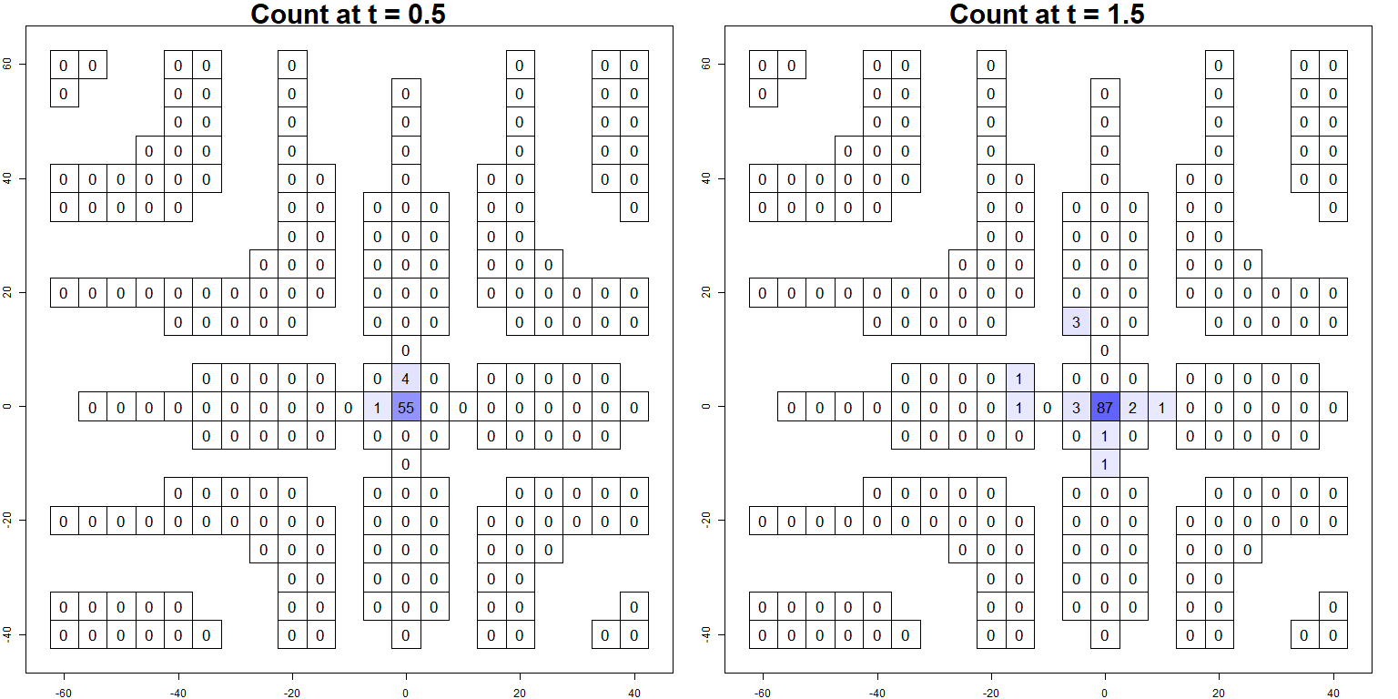
To each trap location we associated a square surrounding region with the trap at the center. The length of the side of each square is the maximum so the squares do not overlap ($5$m in our setting). The so-recorder abundance field is presented in Figure 1. For the Snapshot model, each square is associated with a snapshot-take region. For the Capture model, the union of the squares form the capture domain, and we retain such discretization for the simulation algorithm.

7.4 Implementation and Results

We are interested in the spread of a species in small time scale. Therefore, we use Brownian motion with advection for the underlying trajectory in the Snapshot model and the free-trajectory in the Capture model: $X(t)=v(t-t_{0})+\sigma B(t-t_{0})$, where $B$ is a standard $2$-dimensional Brownian motion, $v=(v_{x},v_{y})\in\mathbb{R}^{2}$ is the advection vector, and $\sigma>0$ is a spread parameter, i.e., the standard deviation of the Brownian term. Parameter $\sigma$ controls the diffusivity of the general abundance: the greater it is, the further the population spreads within a given time. The advection vector $v$ describes a net average population movement preference towards some direction. The final number of scalar parameters to be estimated for each model is $4$: $\sigma,v_{x},v_{y}$ for the movement, and one additional parameter that characterizes the observation process: detection probability $p$ in the Snapshot model and the parameter $\alpha$ in the Capture model. We use a $1$-minute-resolution time grid $(\Delta t=1/60)$ for the discrete-time grid for the Capture model. For details of implementation, see Appendix A.

7.4.1 MGLE model fitting results

Results of fitting our models to the fly data with MGLE are presented in Tables 1 and 2. Table 1 presents the point estimates for the parameters of each model, as well as the maximum of the Gaussian log-likelihood and its continuity-corrected version. Table 2 shows the associated $95\%$ confidence intervals. For the EcoDiff model only, we also compute the exact MLEs, since its likelihood of this model is tractable; see Table 3. Note that this maximum log-likelihood must be compared ith the continuity-corrected log-likelihoods obtained with MGLE. Since all models have $4$ parameters to be fitted, there is no need of computing the AIC for model comparison: comparing the log-likelihoods is enough.

MGLE (point estimates)
Model $\hat{\sigma}$ $\hat{v_{x}}$ $\hat{v_{y}}$ $\hat{p}$ $\hat{\alpha}$ $\log(\mathcal{L})$ c.c. $\log(\mathcal{L})$
EcoDiff $2.849$ $-1.280$ $1.805$ $0.0294$ $-$ $2274.47$ $-210.714$
Snapshot $2.852$ $-1.277$ $1.802$ $0.0290$ $-$ $2273.362$ $-211.569$
Capture $3.140$ $-1.897$ $2.499$ $-$ $0.03241$ $2334.782$ $-148.619$
Table 1: MGLE results for the Rover fly data
MGLE $95\%$ confidence intervals
Model $\hat{\sigma}$ $\hat{v_{x}}$ $\hat{v_{y}}$ $\hat{p}$ $\hat{\alpha}$
EcoDiff $[2.758,2.940]$ $[-1.557,-1.003]$ $[1.578,2.032]$ $[0.0262,0.0326]$ $-$
Snapshot $[2.761,2.943]$ $[-1.552,-1.001]$ $[1.575,2.028]$ $[0.0259,0.0321]$ $-$
Capture $[3.043,3.237]$ $[-2.249,-1.546]$ $[2.219,2.779]$ $-$ $[0.0285,0.0363]$
Table 2: MGLE confidence intervals for the Rover Fly data
EcoDiff exact MLEs
$\hat{\sigma}$ $\hat{v_{x}}$ $\hat{v_{y}}$ $\hat{p}$ $\log(\mathcal{L})$
Point estimates $2.075$ $-0.302$ $0.361$ $0.0142$ $-138.733$
$95\%$ CI $[1.889,2.262]$ $[-0.675,0.071]$ $[-0.012,0.733]$ $[0.0120,0.0164]$ $-$
Table 3: Exact MLEs of the EcoDiff model for the Rover fly data

According to the MGLE, the Capture model fits the data better than the other two models according to the obtained maximum likelihood, continuity-corrected or not. This is not a big surprise, since the Capture model is a more loyal representation of the studied spreading/capturing process, considering in particular the cumulative-in-time information of the count. Under the Capture model, the estimate of the spread parameter $\sigma$ was about $10\%$ higher than under the Snapshot and EcoDiff models, while the estimates of the magnitude of the components of the advection vector $v$ were about $40-50\%$ higher. This result was also expected, since fitting a model which assumes free individuals (Snapshot and EcoDiff) to a data set where individuals may be retained in traps will naturally underestimate the spread and general movement potential of the population.

We note that estimates under the EcoDiff and the Snapshot models hardly differ, and that the EcoDiff log-likelihood is barely better. An explanation for this is the following: with the MGLE method, both models assume a Gaussian distribution with the same mean vector (see Section 7.2), but a different covariance matrix; it is diagonal in the EcoDiff. When using parameters values similar to the estimated for our data, the theoretical covariances under the Snapshot model are small, thus the Snapshot model almost reduces to the EcoDiff. But with different parameters values, the Snapshot model may propose higher auto-correlation values, implying thus a bigger discrepancy between the likelihood of Snapshot and EcoDiff models. This is shown in Table 4, where three different parameter settings are proposed, the associated maximum absolute space-time auto-correlation for the Snapshot model is showed, and the Gaussian log-likelihoods of both models over the fly data are compared.

Comparison between EcoDiff and Snapshot models
Values of $(\sigma,v_{x},v_{y},p)$ Snapshot max. abs. auto-corr. EcoDiff $\log(\mathcal{L})$ Snapshot $\log(\mathcal{L})$
$(2.85,-1.28,1.8,0.03)$ $0.0092$ $2133.61$ $2132.37$
$(10,-5,5,0.9)$ $0.0649$ $-2914.79$ $-8062.40$
$(5,0,0,0.5)$ $0.0982$ $-557.80$ $-2421.74$
Table 4: Effects of different parameter values on the auto-correlation of the Snapshot model and on the Gaussian log-likelihood in EcoDiff and Snapshot models over the fly data. The second column gives the maximum absolute correlation among different space-time locations under the Snapshot model. The last two columns present the continuous Gaussian log-likelihood of each model.

Comparison of the MGLEs and the exact MLEs for the EcoDiff model provides insights on the limitations of the MGLE approach and the relevance of these estimates for interpreting the fly data. There is a huge difference between the estimates from MLE and MGLE. The MLE point estimates are substantially smaller than the MGLE point estimates: the spread parameter is $35\%$ smaller, the two components of the advection vector are between $20$ and $25\%$ of the MGLE estimates, and detection probability is reduced by half. The CIs under the two methods don’t overlap for any of the parameters.

Interestingly, the EcoDiff model with MLE method yields a higher value of the maximized log-likelihood than the continuity-corrected log-likelihood of all the models with the MGLE method, and it is thus the best model here explored in terms of AIC. It is not clear whether doing Snapshot and Capture models with an exact MLE will improve the results, nor if the parameter estimates will also be significantly obtained to the MGLEs. The difference in the MLE and MGLE estimates could be given by the complexity of the models, some particularity of the data set, and/or a poor Gaussian approximation for a sample of size $N=5644$. To elucidate this, we devised a simulation study, which we describe next.

7.4.2 Simulation-based validation of the MGLE method

We conducted a simulation study with the same space-time configuration as in the actual fly data. We gauged the quality of the estimates for $N=10^{2},10^{3},5644,10^{4},10^{5}$ and for different values of the spread parameter $\sigma=2,5,10$, representing slow, medium and fast spread. We kept a small advection similar as estimated from the real data set ($v=(-1,1)$), and chose a small detection probability $p=0.1$ for the EcoDiff and the Snapshot models, and $\alpha=0.1$ for the Capture model. We simulated $300$ data sets for each configuration and model and used MGLE for model fitting. For comparison, we also used exact MLE for the EcoDiff model.

Results of the MGLE method are shown in Table 5 for the Snapshot, Table 6 for the Capture and Table 7 for the EcoDiff model. For each configuration, the average of the point estimates over the $300$ simulated data sets is presented, and the coverage probability in a $95\%$ Gaussin CI is given in the following parentheses. In the final column we give the coverage of a joint $95\%$ Gaussian confidence ellipsoid. Finally, results for the exact MLE for the EcoDiff model are presented in Table 8.

MGLE for Snapshot, $(\sigma,v_{x},v_{y},p)=(2,-1,1,0.1)$
$N$ $\hat{\sigma}_{mean}$ $\hat{v}_{x,mean}$ $\hat{v}_{y,mean}$ $\hat{p}_{mean}$ ellipsoid $CP$
$10^{2}$ 1.222 (0.06) -1.137 (0.323) 1.032 (0.227) 0.133 (0.727) 0.007
$10^{3}$ 1.753 (0.053) -0.957 (0.737) 0.961 (0.77) 0.102 (0.94) 0.027
5644 1.897 (0.137) -0.995 (0.917) 0.993 (0.863) 0.1 (0.943) 0.217
$10^{4}$ 1.934 (0.25) -0.996 (0.923) 0.999 (0.943) 0.1 (0.937) 0.37
$10^{5}$ 1.989 (0.727) -1.001 (0.957) 1.001 (0.95) 0.1 (0.937) 0.837
MGLE for Snapshot, $(\sigma,v_{x},v_{y},p)=(5,-1,1,0.1)$
$N$ $\hat{\sigma}_{mean}$ $\hat{v}_{x,mean}$ $\hat{v}_{y,mean}$ $\hat{p}_{mean}$ ellipsoid $CP$
$10^{2}$ 2.857 (0.003) -0.898 (0.247) 0.885 (0.157) 0.189 (0.163) 0
$10^{3}$ 3.964 (0.01) -0.973 (0.3) 0.983 (0.283) 0.112 (0.633) 0
5644 4.46 (0.02) -0.99 (0.41) 1.009 (0.403) 0.099 (0.913) 0
$10^{4}$ 4.593 (0.033) -1.034 (0.513) 1.032 (0.55) 0.099 (0.86) 0.007
$10^{5}$ 4.902 (0.033) -1.009 (0.853) 1 (0.873) 0.099 (0.787) 0.03
MGLE for Snapshot, $(\sigma,v_{x},v_{y},p)=(10,-1,1,0.1)$
$N$ $\hat{\sigma}_{mean}$ $\hat{v}_{x,mean}$ $\hat{v}_{y,mean}$ $\hat{p}_{mean}$ ellipsoid $CP$
$10^{2}$ 5.716 (0) -0.617 (0.077) 0.74 (0.1) 0.318 (0.013) 0
$10^{3}$ 8.221 (0.013) -0.728 (0.2) 0.761 (0.18) 0.137 (0.027) 0
5644 9.082 (0.013) -0.802 (0.377) 0.723 (0.31) 0.104 (0.74) 0
$10^{4}$ 9.272 (0.033) -0.877 (0.36) 0.788 (0.377) 0.101 (0.9) 0
$10^{5}$ 9.88 (0.16) -0.995 (0.76) 0.998 (0.77) 0.1 (0.837) 0.127
Table 5: MGLE of Snapshot parameters on simulation study. Results over $300$ simulations.
MGLE for Capture, $(\sigma,v_{x},v_{y},\alpha)=(2,-1,1,0.1)$
$N$ $\hat{\sigma}_{mean}$ $\hat{v}_{x,mean}$ $\hat{v}_{y,mean}$ $\hat{\alpha}_{mean}$ ellipsoid $CP$
$10^{2}$ 0.969 (0.051) -1.301 (0.207) 1.308 (0.191) 0.13 (0.828) 0.02
$10^{3}$ 1.697 (0.086) -1.009 (0.699) 1.058 (0.637) 0.101 (0.93) 0.047
5644 1.882 (0.172) -0.981 (0.855) 0.991 (0.867) 0.1 (0.926) 0.246
$10^{4}$ 1.916 (0.293) -0.984 (0.879) 0.984 (0.891) 0.1 (0.938) 0.363
$10^{5}$ 1.986 (0.812) -1.004 (0.934) 1.001 (0.969) 0.1 (0.953) 0.891
MGLE for Capture, $(\sigma,v_{x},v_{y},\alpha)=(5,-1,1,0.1)$
$N$ $\hat{\sigma}_{mean}$ $\hat{v}_{x,mean}$ $\hat{v}_{y,mean}$ $\hat{\alpha}_{mean}$ ellipsoid $CP$
$10^{2}$ 2.46 (0.01) -0.808 (0.268) 0.762 (0.224) 0.204 (0.275) 0
$10^{3}$ 3.756 (0.007) -0.94 (0.295) 0.86 (0.353) 0.115 (0.647) 0
5644 4.278 (0.007) -0.966 (0.553) 0.929 (0.485) 0.1 (0.895) 0.003
$10^{4}$ 4.423 (0.024) -0.994 (0.539) 0.948 (0.539) 0.099 (0.868) 0
$10^{5}$ 4.853 (0.051) -0.987 (0.851) 0.995 (0.8) 0.099 (0.817) 0.044
MGLE for Capture, $(\sigma,v_{x},v_{y},\alpha)=(10,-1,1,0.1)$
$N$ $\hat{\sigma}_{mean}$ $\hat{v}_{x,mean}$ $\hat{v}_{y,mean}$ $\hat{\alpha}_{mean}$ ellipsoid $CP$
$10^{2}$ 4.771 (0) -0.747 (0.094) 0.321 (0.109) 0.369 (0.027) 0
$10^{3}$ 7.786 (0.004) -1.157 (0.156) 1.021 (0.164) 0.149 (0.012) 0
5644 8.796 (0.031) -0.651 (0.246) 0.96 (0.266) 0.106 (0.711) 0
$10^{4}$ 9.016 (0.008) -0.73 (0.387) 0.82 (0.383) 0.102 (0.906) 0
$10^{5}$ 9.704 (0.078) -0.954 (0.715) 0.958 (0.711) 0.099 (0.77) 0.027
Table 6: MGLE of Capture parameters on simulation study. Results over $300$ simulations.
MGLE for EcoDiff, $(\sigma,v_{x},v_{y},p)=(2,-1,1,0.1)$
$N$ $\hat{\sigma}_{mean}$ $\hat{v}_{x,mean}$ $\hat{v}_{y,mean}$ $\hat{p}_{mean}$ ellipsoid $CP$
$10^{2}$ 1.238 (0.087) -1.208 (0.313) 1.232 (0.297) 0.139 (0.753) 0
$10^{3}$ 1.755 (0.053) -0.988 (0.72) 0.967 (0.707) 0.102 (0.93) 0.027
5644 1.901 (0.163) -0.996 (0.887) 0.987 (0.893) 0.1 (0.927) 0.243
$10^{4}$ 1.934 (0.273) -1.002 (0.933) 0.996 (0.903) 0.1 (0.943) 0.427
$10^{5}$ 1.991 (0.757) -1.004 (0.923) 1.002 (0.957) 0.1 (0.933) 0.843
MGLE for EcoDiff, $(\sigma,v_{x},v_{y},p)=(5,-1,1,0.1)$
$N$ $\hat{\sigma}_{mean}$ $\hat{v}_{x,mean}$ $\hat{v}_{y,mean}$ $\hat{p}_{mean}$ ellipsoid $CP$
$10^{2}$ 2.812 (0) -0.862 (0.257) 1.027 (0.227) 0.214 (0.18) 0
$10^{3}$ 3.928 (0.003) -0.956 (0.303) 0.946 (0.313) 0.115 (0.563) 0
5644 4.505 (0.02) -1.09 (0.39) 1.021 (0.373) 0.101 (0.927) 0
$10^{4}$ 4.621 (0.047) -0.982 (0.547) 1.006 (0.573) 0.099 (0.87) 0
$10^{5}$ 4.911 (0.05) -1.008 (0.847) 1 (0.857) 0.099 (0.78) 0.04
MGLE for EcoDiff, $(\sigma,v_{x},v_{y},p)=(10,-1,1,0.1)$
$N$ $\hat{\sigma}_{mean}$ $\hat{v}_{x,mean}$ $\hat{v}_{y,mean}$ $\hat{p}_{mean}$ ellipsoid $CP$
$10^{2}$ 5.748 (0.003) -1.089 (0.117) 1.199 (0.123) 0.445 (0.007) 0
$10^{3}$ 8.211 (0.007) -0.78 (0.213) 0.769 (0.15) 0.143 (0.01) 0
5644 9.095 (0.04) -0.873 (0.327) 0.857 (0.33) 0.105 (0.753) 0
$10^{4}$ 9.316 (0.027) -0.846 (0.357) 0.798 (0.4) 0.101 (0.89) 0.003
$10^{5}$ 9.863 (0.107) -0.984 (0.79) 0.978 (0.783) 0.1 (0.89) 0.07
Table 7: MGLE of EcoDiff parameters on simulation study. Results over $300$ simulations.
MLE for EcoDiff, $(\sigma,v_{x},v_{y},p)=(2,-1,1,0.1)$
$N$ $\hat{\sigma}_{mean}$ $\hat{v}_{x,mean}$ $\hat{v}_{y,mean}$ $\hat{p}_{mean}$ ellipsoid $CP$
$10^{2}$ 1.859 (0.967) -1.067 (0.947) 1.062 (0.92) 0.101 (0.917) 0.873
$10^{3}$ 1.99 (0.957) -1.014 (0.957) 1.004 (0.94) 0.1 (0.957) 0.957
5644 1.997 (0.933) -1.007 (0.943) 0.996 (0.957) 0.1 (0.937) 0.933
$10^{4}$ 1.999 (0.96) -1.002 (0.963) 0.998 (0.933) 0.1 (0.953) 0.95
$10^{5}$ 2 (0.937) -1.002 (0.95) 1.001 (0.98) 0.1 (0.943) 0.967
MLE for EcoDiff, $(\sigma,v_{x},v_{y},p)=(5,-1,1,0.1)$
$N$ $\hat{\sigma}_{mean}$ $\hat{v}_{x,mean}$ $\hat{v}_{y,mean}$ $\hat{p}_{mean}$ ellipsoid $CP$
$10^{2}$ 4.693 (0.887) -0.959 (0.94) 1.068 (0.927) 0.101 (0.927) 0.853
$10^{3}$ 4.957 (0.953) -1.017 (0.933) 0.999 (0.947) 0.1 (0.963) 0.947
5644 4.997 (0.967) -1.01 (0.95) 1.011 (0.943) 0.1 (0.953) 0.957
$10^{4}$ 4.998 (0.947) -0.988 (0.933) 0.999 (0.96) 0.1 (0.967) 0.953
$10^{5}$ 5.001 (0.973) -1.004 (0.96) 1 (0.953) 0.1 (0.943) 0.95
MLE for EcoDiff, $(\sigma,v_{x},v_{y},p)=(10,-1,1,0.1)$
$N$ $\hat{\sigma}_{mean}$ $\hat{v}_{x,mean}$ $\hat{v}_{y,mean}$ $\hat{p}_{mean}$ ellipsoid $CP$
$10^{2}$ 9.472 (0.883) -1.023 (0.933) 1.159 (0.923) 0.103 (0.94) 0.887
$10^{3}$ 9.926 (0.937) -0.953 (0.94) 0.991 (0.97) 0.101 (0.96) 0.957
5644 9.999 (0.947) -0.987 (0.96) 0.987 (0.967) 0.1 (0.943) 0.953
$10^{4}$ 10.001 (0.953) -0.982 (0.933) 1.003 (0.947) 0.1 (0.947) 0.95
$10^{5}$ 9.996 (0.963) -1.006 (0.987) 0.996 (0.947) 0.1 (0.953) 0.977
Table 8: MLE of EcoDiff parameters on simulation study. Results over $\leq 300$ simulations.

As a general result, MGLE respects the theory since better estimates are obtained as $N$ grows, suggesting consistent estimation. However, the spread parameter is always underestimated and more so for smaller $N$. For $N=10^{2}$, the average MGLE-based estimate of $\sigma$ is nearly $40\%$ smaller for Snapshot and EcoDiff, and more than $50\%$ for Capture. For EcoDiff with exact MLE with, the underestimation of $\sigma$ is less important and somewhat negligible already for $N=10^{3}$. For all the models and fitting methods, from $N\geq 10^{5}$ the underestimation is less than $3\%$.

Estimates of the advection parameter $v$ were nearly unbiased for $N\geq 10^{3}$ in the low and middle spread scenarios, but were more biased with higher spread, becoming more acceptable for $N\geq 10^{5}$. Estimates of $p$ and $\alpha$ were approximately unbiased for $N\geq 5644$, with some positive bias for smaller $N$.

The negative bias of the spread parameter when using MGLE was usually smaller for slow spread scenarios than for medium-to-high spread scenarios. For instance, for the fly data sample size $N=5644$ and $\sigma=2$, we found a negative bias of about $5-6\%$ for all models, while for $\sigma=5,10$, the negative bias was around $10\%$ for the EcoDiff and Snapshot models and $15\%$ for the Capture model. Similarly, the estimates of $v$, $p$ and $\alpha$ were all better for small or medium spread, but tended to require higher $N$ for high spread scenarios. This general behaviour may be partially explained by the spatial configuration of the traps (Figure 1), for which in small-spread scenarios it is more likely that more individuals will be counted/caught, thus providing more information.

While the bias of MGLE-based estimates was reduced when $N$ grows in all scenarios, the coverage probabilities of the method was in general quite poor and grow only very slowly with $N$. This was more important for mid-to-high levels of spread. Clearly, MGLE yields too small variances for the estimates in our case, and thus too narrow confidence intervals. This pattern was most pronounced for $\sigma$, and that was probably also the reason for why the overall confidence ellipsoids failed to include all true values.

When comparing the MGLE with the MLE results for the EcoDiff model, we note an interesting anomaly with respect to the results presented in Section 7.4.1 for the real data. In the simulation study, MLE performed considerably better in terms of bias and coverage, and the negative bias of $\sigma$ was less important. However, in the analysis of the real data, the MLE yielded a considerably smaller estimate for $\sigma$. This suggests that our real data set may be somewhat atypical with respect to the simulated scenarios for the EcoDiff model. This might suggest that the EcoDiff model is not a good fit for such a data set. We cannot currently say whether the Snapshot and Capture models will present or not the same issue, nor up to which extent.

8 Conclusion and perspectives

Models that define a realistic link between animal counts and the movement of individuals would be considerably valuable, since they could exploit a copious and “cheap” source of data (counts or even detection/non-detection data) for inferences about elusive parameters of animal movement. In this paper, we presented two new models for abundance data that are based on movement modelling without relying on movement data, which we believe may help in this aim.

The theoretical development of these models required the study of the statistical properties of a particular multivariate distribution, the ECM distribution, which counts independent individuals moving across evolving categories over time. We developed two kinds of models: one counting free individuals with detection error, and the other capturing individuals according to an axiomatically defined representation of the capture process. These models present non-trivial space-time auto-correlation structure. We developed simulation algorithms for these models, enabling us to conduct simulation-based assessments of the estimators. For this paper, we developed an approximate method for model fitting based on maximum Gaussian likelihood estimation (MGLE) which respects both mean and auto-correlation structures, and which we use to fit the models to real biological data, comparing the results with those from a traditional EcoDiff model as a benchmark.

We conclude that with the right data, models and fitting methods, it is possible to learn about features of the movement of individuals using only cheap abundance data. This conclusion is supported by our simulation study (Section 7.4.2), which indicates that we can estimate movement parameters with controllable bias even for scenarios with only two time steps. However, one must be aware of the required conditions where our fitting methods and models are more effectively applicable for real data. For example, our MGLE fitting method requires large sample sizes in terms of the number of individuals. In general, there appears to be a persistent negative bias of spread parameters even for very large sample sizes. We suggest to conduct tailor-made simulation studies to validate our methods when applied to any new data set, for one must be able to gauge how well these methods perform for given space-time designs and sample sizes. This permits judgment whether a data is “typical” with respect to the simulated scenarios, or, in other words, whether the model fits the data sufficiently well to reproduce its salient features. We have shown that this may not be the case for the EcoDiff model applied to the fly data set.

Our inability to compute a tractable likelihood remains a challenge, since it complicates statistical inference. The approach of rather replace the likelihood for a simpler one still the most common option (Roques \BOthers., \APACyear2022; Schnoerr \BOthers., \APACyear2016; Malchow \BOthers., \APACyear2024), and whether our covariance-respecting Gaussian approach gives better estimates than more commonly used pseudo-likelihoods or not is a question for future work. One likelihood-free option is to use Approximate Bayesian Computation (ABC) methods (Sisson \BOthers., \APACyear2018, and the references therein), where a data-simulation function is sufficient to do approximate Bayesian inference. ABC methods require the choice of a discrepancy measure between simulated data and real data, which can be constructed using summary statistics which must contain enough information about the parameters of the model. But how to chose such summary statistics in a spread population context is still an area of ongoing research, specially if detection errors or capture rates are considered.

Our work opens many roads for future research, in both theory and practice. From the practical point of view, we emphasize that our models are based on trajectory modelling. Thus, they open up the possibility of integrating in a single analysis both abundance and individual tracking data in a meaningful manner. EcoDiff models and Poisson/Cox point processes are currently the most commonly used models for inference about movement from counts, but they do not share this benefit. In addition, our continuous space-time formulation allows to treat telemetry data with irregular time steps, when this is used in such an integrated data framework. Integrating binary detection/non-detection (a.k.a., presence/absence) data, which is arguably even more widespread than space-time counts, is also theoretically immediate. However, for such data one must be aware of the difficulties in doing a correct statistical analysis. Conceptually, a presence/absence field can be defined analogously as the abundance random measure (17), but replacing the sum by a $\max$, so extreme value theory will likely be important for describing the statistical properties of such a field and for develop adequate model fitting methodologies.

For the modelling part, since in principle we have almost total freedom in the choice of the trajectory models, it is possible to conceive new abundance models with different statistical properties through the use of diverse stochastic processes to describe the movement. OU processes have been used for modelling the movement of territorial animals (Gurarie \BOthers., \APACyear2017; Fleming \BOthers., \APACyear2014\APACexlab\BCnt1; Eisaguirre \BOthers., \APACyear2021). More generally, Itô diffusions provide a rich class of trajectory models which includes Brownian motion and OU processes, with a lot of available literature from the theory of stochastic processes, and for which the connection with diffusion PDEs is well known (Gardiner, \APACyear2009): in the same manner as the Snapshot model with Brownian motion and the EcoDiff model with PDE (62) share the same average behaviour, if we use an Itô diffusion as trajectory model, then the average behaviour of the count field satisfies a Fokker-Planck equation, which is a more general form of advection-diffusion equation (62), where spatial covariates modelling can be included in both the advective and diffusive parts of the equation. These trajectories could be more realistic when the spread of the studied animal population depends strongly on the characteristics of the landscape, e.g., through resource availability, as it has been exploited for instance by Michelot \BOthers. (\APACyear2019).

Another important way in which our models could be extended is by the inclusion of reproduction and death, which of course is crucial in population ecology (Krebs, \APACyear2009). EcoDiff models can consider death and reproduction through the addition of a reaction term to the average PDE (Soubeyrand \BBA Roques, \APACyear2014), but without an explicit underlying movement. It seems that the modelling of individual movement in continuous space and time including reproduction and death processes has hardly ever been developed. While our models do not currently include death and reproduction, the principle of counting or capturing “points” that move could of course also be applied to a more complex movement model where individuals can reproduce and die. However, then we could no longer assume independence between the movement of the individuals, since a new generation’s initial positions must coincide with the reproduction positions of the previous generation of individuals. Thus, a strict ECM distribution does not work for describing such a scenario. Nonetheless, the principle of individuals belonging into evolving categories across time still holds, and both the detection error modelling in the Snapshot and the capture process modelling in the Capture model could be applied regardless of the independence of the movement.

Appendix A Implementation details

Concerning the application Section 7, some technical aspects of the there used methods are here specified.

For the MGLE technique, in order to avoid singular or near-singular covariance matrices, we use a regularisation technique by adding $\epsilon=10^{-6}$ to each component of the Gaussian vector. This multivariate regularised Gaussian likelihood is the one to be maximized in the fitting procedure. Once the maximal continuous likelihood is obtained, a continuity-corrected version of the log-likelihood is computed in order to make this quantity comparable to likelihoods obtained from integer-valued probability distributions such as the EcoDiff model. This continuity correction is done computing $\mathbb{P}(\bm{X}\in[\bm{x}-0.5,\bm{x}+0.5])$, where $\bm{X}$ is the corresponding Gaussian vector and $\bm{x}$ is the integer-valued data vector which the model must fit.

The estimations are obtained using the optim function of R with a L-BFGS-B algorithm. The hessian at the optimal values, which is used to compute estimated $95\%$ Gaussian coverage intervals, is obtained using the hessian function from package numDeriv. We use the dmnorm function from package mnormt for computing the multivariate Gaussian densities, and the pmvnorm function from package TruncatedNormal for computing the corresponding continuity corrected log-likelihood, which is known to be one of the most precise options available in R to compute multivariate Gaussian probabilities (Cao \BOthers., \APACyear2022).

For the EcoDiff exact MLE, due to the high quantity of zero theoretical data (near 00 Poisson rate for some space-time locations), we also used a regularisation technique for the Poisson distribution by adding $\epsilon=10^{-24}$ to the rate of every Poisson component.

The function to simulate and compute the moments of the Capture model are ad-hoc for the Brownian motion case here presented. A method of approximating the bi-variate Gaussian probabilities required in the simulation method of Section 6.2 is used. The method replaces conditional probabilities of the form $\mu_{\tilde{X}(t_{k})|\tilde{X}(t_{k^{\prime}})\in A_{l^{\prime}}}(A_{l})$ by $\mu_{\tilde{X}(t_{k})|\tilde{X}(t_{k^{\prime}})=z_{l^{\prime}}}(A_{l})$, where $z_{l^{\prime}}$ is the center of the square $A_{l^{\prime}}$, for $k\geq k^{\prime}$. From the Markovian property of Brownian motion, such conditional probabilities do not depend upon $t_{k^{\prime}}$ but only on the lag $t_{k}-t_{k^{\prime}}$. This allows to compute the required probabilities faster.

Appendix B Proofs

B.1 Proof of Proposition 2.1

Let us define for each individual $j$, a random array $\bm{O}^{(j)}$ of dimensions $m_{1}\times...\times m_{n}$, for which the component $O_{l_{1},...,l_{n}}^{(j)}$ is $1$ if the individual $j$ does the full path $(l_{1},...,l_{n})$ and 00 if not. Since each individual does one and only one path, all the components of $\bm{O}^{(j)}$ must be null except for one, which is unitary. By definition, the random array $\bm{X}$ is nothing but the sum of these individual-following indicators arrays:

$$\bm{X}=\sum_{j=1}^{N}\bm{O}^{(j)}.$$ (64)

Let $\bm{\xi}=(\xi_{l_{1},...,l_{n}})_{l_{1},...,l_{n}}$ by any array of dimensions $m_{1}\times...\times m_{n}$. We compute thus the characteristic function

$\displaystyle\varphi_{\bm{X}}(\bm{\xi})$ $\displaystyle=\mathbb{E}\left(e^{i\bm{\xi}^{T}\bm{X}}\right)$ (65)
$\displaystyle=\mathbb{E}\left(e^{i\bm{\xi}^{T}\sum_{j=1}^{N}\bm{O}^{(j)}}\right)$
$\displaystyle=\mathbb{E}\left(\prod_{j=1}^{N}e^{i\bm{\xi}^{T}\bm{O}^{(j)}}\right)$
$\displaystyle=\left[\mathbb{E}\left(e^{i\bm{\xi}^{T}\bm{O}}\right)\right]^{N},$

where we have used that the random arrays $(\bm{O}^{(j)})_{j=1,...,N}$ are mutually independent and identically distributed, following the distribution of a reference random array $\bm{O}$. The random array $\bm{O}$ has all its components null except for one, and the probability of $\{O_{l_{1},...,l_{n}}=1\}$ is given by the full path probability $p_{l_{1},...,l_{n}}^{(1,...,n)}$. Hence, we have

$$\mathbb{E}\left(e^{i\bm{\xi}^{T}\bm{O}}\right)=\sum_{l_{1}=1}^{m_{1}}...\sum_{l_{n}=1}^{m_{n}}e^{i\xi_{l_{1},...,l_{n}}}p_{l_{1},...,l_{n}}^{(1,...,n)}.$$ (66)

Using (66) and (65) we obtain the desired result. $\blacksquare$

B.2 Proof of Proposition 2.2

Let $\bm{\xi}=\left(\xi_{k,l}\right)_{k,l}$ be any arrangement in $\mathbb{R}^{m_{1}+...+m_{n}}$. We use the expression of $Q_{k,l}$ as a sum over the margins of $X$ as in (9), having thus

$\displaystyle\varphi_{\bm{Q}}(\bm{\xi})$ $\displaystyle=\mathbb{E}\left(e^{i\sum_{k=1}^{n}\sum_{l_{k}=1}^{m_{k}}\xi_{k,l}Q_{k,l}}\right)$ (67)
$\displaystyle=\mathbb{E}\left(e^{i\sum_{k=1}^{n}\sum_{l=1}^{m_{k}}\xi_{k,l}\sum_{l_{1}=1}^{m_{1}}...\sum_{l_{k-1}=1}^{m_{k-1}}\sum_{l_{k+1}=1}^{m_{k+1}}...\sum_{l_{n}=1}^{m_{n}}X_{l_{1},...,l_{k-1},l,l_{k},...,l_{n}}}\right).$
$\displaystyle=\mathbb{E}\left(e^{i\sum_{l_{1}=1}^{m_{1}}...\sum_{l_{n}=1}^{m_{n}}\left(\sum_{k=1}^{n}\xi_{k,l_{k}}\right)X_{l_{1},...,l_{n}}}\right),$

where we have conveniently re-arranged the multi-sum in the exponential. It turns out that $\varphi_{\bm{Q}}$ can be linked directly to the characteristic function of $\bm{X}$ obtained in Proposition 2.1. The final result is, as desired,

$$\varphi_{\bm{Q}}(\bm{\xi})=\left[\sum_{l_{1}=1}^{m_{1}}...\sum_{l_{n}=1}^{m_{n}}e^{i(\xi_{1,l_{1}}+...+\xi_{n,l_{n}})}p_{l_{1},...,l_{n}}^{(1,...,n)}\right]^{N}.\quad\blacksquare$$ (68)

B.3 Proof of Proposition 2.3

Let $\vec{\xi}=(\xi_{1},...,\xi_{m_{k}})\in\mathbb{R}^{m_{k}}$. The characteristic function of the random vector $\vec{Q}_{k}$ evaluated at $\vec{\xi}$ can be simply obtained by evaluating the characteristic function of the full random arrangement $\bm{Q}$, in an arrangement $\bm{\tilde{\xi}}=(\tilde{\xi}_{k^{\prime},l})_{k^{\prime},l}$ defined such that $\tilde{\xi}_{k^{\prime},l}=0$ if $k^{\prime}\neq k$ and $\tilde{\xi}_{k,l}=\xi_{l}$ for every $l=1,...,m_{k}$. Thus,

$\displaystyle\varphi_{\vec{Q}_{k}}(\vec{\xi})$ $\displaystyle=\varphi_{\bm{Q}}(\bm{\tilde{\xi}})$ (69)
$\displaystyle=\left[\sum_{l_{1}=1}^{m_{1}}...\sum_{l_{n}=1}^{m_{n}}e^{i(\tilde{\xi}_{1,l_{1}}+...+\tilde{\xi}_{n,l_{n}})}p_{l_{1},...,l_{n}}^{(1,...,n)}\right]^{N}$
$\displaystyle=\left[\sum_{l_{1}=1}^{m_{1}}...\sum_{l_{n}=1}^{m_{n}}e^{i\xi_{l_{k}}}p_{l_{1},...,l_{n}}^{(1,...,n)}\right]^{N}$
$\displaystyle=\left[\sum_{l_{k}=1}^{m_{k}}e^{i\xi_{l_{k}}}\sum_{l_{1}=1}^{m_{1}}...\sum_{l_{k-1}}^{m_{k-1}}\sum_{l_{k+1}=1}^{m_{k+1}}...\sum_{l_{n}=1}^{m_{n}}p_{l_{1},...,l_{n}}^{(1,...,n)}\right]^{N}.$

Now, from the projectivity condition (4) on the sub-paths probabilities, one must have

$$\sum_{l_{1}=1}^{m_{1}}...\sum_{l_{k-1}}^{m_{k-1}}\sum_{l_{k+1}=1}^{m_{k+1}}...\sum_{l_{n}}^{m_{n}}p_{l_{1},...,l_{n}}^{(1,...,n)}=p_{l_{k}}^{(k)}.$$ (70)

Using (70) in (69),we obtain

$$\varphi_{\vec{Q}_{k}}(\vec{\xi})=\left[\sum_{l_{k}=1}^{m_{k}}e^{i\xi_{l_{k}}}p_{l_{k}}^{(k)}\right]^{N},$$ (71)

which coincides with the characteristic function of a multinomial random vector of size $N$ and probabilities vector $(p_{1}^{(k)},...,p_{m_{k}}^{(k)})$. $\blacksquare$

B.4 Proof of Proposition 2.4

We remind that for two random vectors $\vec{X}$ and $\vec{Y}$ tanking values in $\mathbb{R}^{m}$ and $\mathbb{R}^{n}$ respectively, the conditioned characteristic function $\varphi_{\vec{X}|\vec{Y}=\vec{y}}$ satisfies

$$\varphi_{\vec{X},\vec{Y}}(\vec{\xi},\vec{\eta})=\int_{\mathbb{R}^{n}}\varphi_{\vec{X}|\vec{Y}=\vec{y}}(\vec{\xi})e^{i\vec{\eta}^{T}\vec{y}}d\mu_{\vec{Y}}(\vec{y}),\quad\vec{\xi}\in\mathbb{R}^{m},\vec{\eta}\in\mathbb{R}^{n}.$$ (72)

In our case, consider $\tilde{k}\neq k$. Using that $\vec{Q}_{k}$ follows a multinomial distribution (Proposition 2.3) we can use the principle (72) and conclude that the joint characteristic function of $\vec{Q}_{\tilde{k}}$ and $\vec{Q}_{k}$ satisfies

$\displaystyle\varphi_{\vec{Q}_{\tilde{k}},\vec{Q}_{k}}(\vec{\xi},\vec{\eta})$ $\displaystyle=\sum_{\begin{subarray}{c}\vec{q}\in\{0,...,N\}^{m_{k}}\\ sum(\vec{q})=N\end{subarray}}\varphi_{\vec{Q}_{\tilde{k}}|\vec{Q}_{k}=\vec{q}}(\vec{\xi})e^{i\vec{\eta}^{T}\vec{q}}\mathbb{P}\left(\vec{Q}_{k}=\vec{q}\right)$ (73)
$\displaystyle=\sum_{\begin{subarray}{c}\vec{q}\in\{0,...,N\}^{m_{k}}\\ sum(\vec{q})=N\end{subarray}}\varphi_{\vec{Q}_{\tilde{k}}|\vec{Q}_{k}=\vec{q}}(\vec{\xi})e^{i\vec{\eta}^{T}\vec{q}}\frac{N!}{q_{1}!...q_{m_{k}}!}\left(p_{1}^{(k)}\right)^{q_{1}}...\left(p_{l_{m_{k}}}^{(k)}\right)^{q_{m_{k}}},$

for every $\vec{\xi}=(\xi_{1},...,\xi_{m_{\tilde{k}}})\in\mathbb{R}^{m_{\tilde{k}}}$, and every $\vec{\eta}=(\eta_{1},...,\eta_{m_{k}})\in\mathbb{R}^{m_{k}}$. Here we denoted $sum(\vec{q})=q_{1}+...+q_{m_{k}}$. On the other hand, an explicit expression for $\varphi_{\vec{Q}_{\tilde{k}},\vec{Q}_{k}}$ can be obtained in a similar manner as the marginal characteristic function $\varphi_{\vec{Q}_{k}}$ obtained in the proof of Proposition 2.3, that is, by considering an arrangement with convenient null components for evaluating $\varphi_{\bm{Q}}$ and using the projectivity condition (4). The final result (details are left to the reader) is

$$\varphi_{\vec{Q}_{\tilde{k}},\vec{Q}_{k}}(\vec{\xi},\vec{\eta})=\left[\sum_{l_{\tilde{k}}=1}^{m_{\tilde{k}}}\sum_{l_{k}=1}^{m_{k}}e^{i(\xi_{l_{\tilde{k}}}+\eta_{l_{k}})}p_{l_{k},l_{\tilde{k}}}^{(k,\tilde{k})}\right]^{N},$$ (74)

Using the factorisation $p_{l_{k},l_{\tilde{k}}}^{(k,\tilde{k})}=p_{l_{\tilde{k}}|l_{k}}^{(\tilde{k}|k)}p_{l_{k}}^{(k)}$ and the multinomial theorem, we obtain

$\displaystyle\varphi_{\vec{Q}_{\tilde{k}},\vec{Q}_{k}}(\vec{\xi},\vec{\eta})$ $\displaystyle=\left[\sum_{l_{k}=1}^{m_{k}}e^{i\eta_{l_{k}}}p_{l_{k}}^{(k)}\sum_{l_{\tilde{k}}=1}^{m_{\tilde{k}}}e^{i\xi_{l_{\tilde{k}}}}p_{l_{\tilde{k}}|l_{k}}^{(\tilde{k}|k)}\right]^{N}$ (75)
$\displaystyle=\sum_{\begin{subarray}{c}\vec{q}\in\{0,...,N\}^{m_{k}}\\ sum(\vec{q})=N\end{subarray}}\frac{N!}{q_{1}!...q_{m_{k}}!}e^{i\vec{\eta}^{T}\vec{q}}\left(p_{1}^{(k)}\right)^{q_{1}}...\left(p_{l_{m_{k}}}^{(k)}\right)^{q_{m_{k}}}\prod_{l_{k}=1}^{m_{k}}\left[\sum_{l_{\tilde{k}}=1}^{m_{\tilde{k}}}e^{i\xi_{l_{\tilde{k}}}}p_{l_{\tilde{k}}|l_{k}}^{(\tilde{k}|k)}\right]^{q_{l_{k}}}.$

Comparing term-by-term expressions (73) and (75), we conclude

$$\varphi_{\vec{Q}_{\tilde{k}}|\vec{Q}_{k}=\vec{q}}(\vec{\xi})=\prod_{l_{k}=1}^{m_{k}}\left[\sum_{l_{\tilde{k}}=1}^{m_{\tilde{k}}}e^{i\xi_{l_{\tilde{k}}}}p_{l_{\tilde{k}}|l_{k}}^{(\tilde{k}|k)}\right]^{q_{l_{k}}}.$$ (76)

Note that the comparing term-by-term method is justified from the linear independence of the functions $\eta\in\mathbb{R}^{m_{k}}\mapsto e^{i\eta^{T}\vec{q}}$ for $\vec{q}\in\{0,...,N\}^{m_{k}}$. Characteristic function (76) is the product of $m_{k}$ multinomial characteristic functions, each one with the desired sizes and probabilities vectors. $\blacksquare$

B.5 Proof of Proposition 2.5

From Proposition 2.3, since $\vec{Q}_{k}$ is multinomial, one has immediately $\mathbb{E}(Q_{k,l})=Np_{l}^{(k)}$ for every $l\in\{1,...,m_{k}\}$, which proves the mean structure (13). On the other hand, since $\mathbb{E}(Q_{k,l}Q_{k,\tilde{l}})=\mathbb{C}ov(Q_{k,l}\ ,\ Q_{k,\tilde{l}})+\mathbb{E}(Q_{k,l})\mathbb{E}(Q_{k,\tilde{l}})$, and using the covariance matrix of a multinomial random vector, we have

$$\mathbb{E}(Q_{k,l}^{2})=Np_{l}^{(k)}(1-p_{l}^{(k)})+N^{2}\left(p_{l}^{(k)}\right)^{2}=Np_{l}^{(k)}+N(N-1)\left(p_{l}^{(k)}\right)^{2},$$ (77)

and

$$\mathbb{E}(Q_{k,l}Q_{k,\tilde{l}})=-Np_{l}^{(k)}p_{\tilde{l}}^{(k)}+N^{2}p_{l}^{(k)}p_{\tilde{l}}^{(k)}=N(N-1)p_{l}^{(k)}p_{\tilde{l}}^{(k)}$$ (78)

when $l\neq\tilde{l}$, which proves the case $k=\tilde{k}$ in Eq. (14).

For the case $k\neq\tilde{k}$, we use Proposition 2.4 and the properties of conditional expectations:

$\displaystyle\mathbb{E}(Q_{k,l}Q_{\tilde{k},\tilde{l}})$ $\displaystyle=\mathbb{E}\left(Q_{k,l}\mathbb{E}\left(Q_{\tilde{k},\tilde{l}}\ \big{|}\ \vec{Q}_{k}\right)\right)$ (79)
$\displaystyle=\mathbb{E}\left(Q_{k,l}\sum_{l^{\prime}=1}^{m_{k}}Q_{k,l^{\prime}}p_{\tilde{l}|l^{\prime}}^{(\tilde{k}|k)}\right)$ $\displaystyle\begin{subarray}{c}\hbox{(expectation of sum of indep.}\\ \hbox{multinomials)}\end{subarray}$
$\displaystyle=\sum_{l^{\prime}=1}^{m_{k}}\mathbb{E}\left(Q_{k,l}Q_{k,l^{\prime}}\right)p_{\tilde{l}|l^{\prime}}^{(\tilde{k}|k)}$
$\displaystyle=\sum_{l^{\prime}=1}^{m_{k}}\left(\delta_{l,l^{\prime}}Np_{l}^{(k)}+N(N-1)p_{l}^{(k)}p_{l^{\prime}}^{(k)}\right)p_{\tilde{l}|l^{\prime}}^{(\tilde{k}|k)}$ (expressions (77) and (78))
$\displaystyle=Np_{l}^{(k)}p_{\tilde{l}|l}^{(\tilde{k}|k)}+N(N-1)p_{l}^{(k)}\sum_{l^{\prime}=1}^{m_{k}}p_{l^{\prime},\tilde{l}}^{(k,\tilde{k})}$ $\displaystyle\begin{subarray}{c}\hbox{(split the sum and use conditional }\\ \hbox{probability products)}\end{subarray}$
$\displaystyle=Np_{l,\tilde{l}}^{(k,\tilde{k})}+N(N-1)p_{l}^{(k)}p_{\tilde{l}}^{(\tilde{k})},$ (conditional probability products and projectivity condition (4) )(conditional probability products and projectivity condition (4) )\displaystyle\begin{subarray}{c}\hbox{(conditional probability products }\\ \hbox{and projectivity condition \eqref{Eq:ProjSubPathProbs} )}\end{subarray}

which proves the desired result. $\blacksquare$

B.6 Proof of Proposition 3.1

Let $\vec{\xi}=(\xi_{1},...,\xi_{n})\in\mathbb{R}^{n}$. We compute directly:

$\displaystyle\varphi_{\Phi_{t_{1}}(A_{1}),...,\Phi_{t_{n}}(A_{n})}(\vec{\xi})$ $\displaystyle=\mathbb{E}\left(e^{i\sum_{k=1}^{n}\xi_{k}\Phi_{t_{k}}(A_{k})}\right)$ (80)
$\displaystyle=\mathbb{E}\left(e^{i\sum_{j=1}^{N}\sum_{k=1}^{n}\xi_{k}\delta_{X_{j}(t_{k})}(A_{k})}\right)$
$\displaystyle=\left[\mathbb{E}\left(e^{i\sum_{k=1}^{n}\xi_{k}\delta_{X(t_{k})}(A_{k})}\right)\right]^{N},$

where we have used the iid Assumption 3.1 on the trajectories. Now, $\mathbb{E}\left(e^{i\sum_{k=1}^{n}\xi_{k}\delta_{X(t_{k})}(A_{k})}\right)$ is the characteristic function of the random vector with binary components $\left(\delta_{X(t_{1})}(A_{1}),...,\delta_{X(t_{n})}(A_{n})\right)$. This random vector can, in principle, take any possible value in the set $\{0,1\}^{n}$, the probability of each value being

$\displaystyle\mathbb{P}\left(\left(\delta_{X(t_{1})}(A_{1}),...,\delta_{X(t_{n})}(A_{n})\right)=\vec{j}\right)$ $\displaystyle=\mathbb{P}\left(X(t_{1})\in A_{1}^{(1-j_{1})c},X(t_{2})\in A_{2}^{(1-j_{2})c},...,X(t_{n})\in A_{n}^{(1-j_{n})c}\right)$ (81)
$\displaystyle=\mu_{X(t_{1}),...,X(t_{n})}\left(A_{1}^{(1-j_{1})c}\times...\times A_{n}^{(1-j_{n})c}\right),$

for all $\vec{j}=(j_{1},...,j_{n})\in\{0,1\}^{n}$. One has then,

$$\mathbb{E}\left(e^{i\sum_{k=1}^{n}\xi_{k}\delta_{X(t_{k})}(A_{k})}\right)=\sum_{\vec{j}\in\{0,1\}^{n}}e^{i\xi^{T}\vec{j}}\mu_{X(t_{1}),...,X(t_{n})}\left(A_{1}^{(1-j_{1})c}\times...\times A_{n}^{(1-j_{n})c}\right).$$ (82)

Eq. (80) together with Eq. (82) lead to the desired result. $\blacksquare$

B.7 Proof of Proposition 4.1

We first use a Lemma concerning the probability generating function of an ECM random arrangement.

Lemma B.1.

The probability generating function of an ECM random arrangement $\bm{Q}$, with number of individuals $N$, number of times $n$, with $m_{k}$ categories at each time $k$, and with full path probabilities $p_{l_{1},...,l_{n}}^{(1,..,n)}$ is given by

$$G_{\bm{Q}}(\bm{z})=\left[\sum_{l_{1}=1}^{m_{1}}...\sum_{l_{n}=1}^{m_{n}}p_{l_{1},...,l_{n}}^{(1,...,n)}\prod_{k=1}^{n}z_{k,l_{k}}\right]^{N},$$ (83)

for every arrangement of complex numbers $\bm{z}=(z_{k,l})_{k,l}$ such that $|z_{k,l}|\leq 1$ for every $k,l$.

Proof of Lemma B.1: It is enough to verify for arrangements $\bm{z}=(z_{k,l})_{k,l}$ such that $z_{k,l}\neq 0$. Express every complex number $z_{k,l}$ in the form $z_{k,l}=e^{\log(r_{k,l})+i\xi_{k,l}}$, with $r_{k,l}=|z_{k,l}|>0$. Then, use the same arguments as in the proof of Proposition (2.2) presented in Appendix B.2 for the characteristic function $\varphi_{\bm{Q}}$, which is based on expressing $\bm{Q}$ in terms of the underlying multinomial random array $\bm{X}$. $\blacksquare$

Proof of Proposition 4.1: Let us compute the characteristic function of the random arrangement $\bm{\tilde{Q}}$. Let $\bm{\xi}=(\xi_{k,l})_{k,l}$ be an arrangement in $\mathbb{R}^{(m_{1}+1)+...+(m_{k}+1)}$. Then,

$\displaystyle\varphi_{\bm{\tilde{Q}}}(\bm{\xi})$ $\displaystyle=\mathbb{E}\left(e^{i\sum_{k=1}^{n}\sum_{l=1}^{m_{k}+1}\tilde{Q}_{k,l}\xi_{k,l}}\right)$ (84)
$\displaystyle=\mathbb{E}\left(\mathbb{E}\left(e^{i\sum_{k=1}^{n}\left(R_{t_{k}}\xi_{k,m_{k}+1}+\sum_{l=1}^{m_{k}}Q_{t_{k}}(A_{k,l})\xi_{k,l}\right)}\ \big{|}\ \Phi\right)\right)$
$\displaystyle=\mathbb{E}\left(\prod_{k=1}^{n}\mathbb{E}\left(e^{i\left(R_{t_{k}}\xi_{k,m_{k}+1}+\sum_{l=1}^{m_{k}}Q_{t_{k}}(A_{k,l})\xi_{k,l}\right)}\ \big{|}\ \Phi\right)\right),$

where we have used the properties of the conditional expectation and the conditional independence condition at different times i. Let us now compute the inner conditional expectations

$\displaystyle\mathbb{E}\left(e^{i\left(R_{t_{k}}\xi_{k,m_{k}+1}+\sum_{l=1}^{m_{k}}Q_{t_{k}}(A_{k,l})\xi_{k,l}\right)}\ \big{|}\ \Phi\right)$ $\displaystyle=\mathbb{E}\left(e^{i\left(N\xi_{k,m_{k}+1}+\sum_{l=1}^{m_{k}}Q_{t_{k}}(A_{k,l})(\xi_{k,l}-\xi_{k,m_{k}+1})\right)}\ \big{|}\ \Phi\right)$ (85)
$\displaystyle=e^{iN\xi_{k,m_{k}+1}}\mathbb{E}\left(e^{i\sum_{l=1}^{m_{k}}Q_{t_{k}}(A_{k,l})(\xi_{k,l}-\xi_{k,m_{k}+1})}\ \big{|}\ \Phi\right)$
$\displaystyle=e^{iN\xi_{k,m_{k}+1}}\prod_{l=1}^{m_{k}}\mathbb{E}\left(e^{iQ_{t_{k}}(A_{k,l})(\xi_{k,l}-\xi_{k,m_{k}+1})}\ \big{|}\ \Phi\right)$
$\displaystyle=e^{iN\xi_{k,m_{k}+1}}\prod_{l=1}^{m_{k}}\left[pe^{i(\xi_{k,l}-\xi_{k,m_{k}+1})}+1-p\right]^{\Phi_{t_{k}}(A_{k,l})}.$

Let us introduce the sets $A_{k,m_{k}+1}:=\mathbb{R}^{d}\setminus\left(\bigcup_{l=1}^{m_{k}}A_{k,l}\right)$ for every $k=1,...,n$. We have then

$$N=\Phi_{t_{k}}(A_{k,m_{k}+1})+\sum_{l=1}^{m_{k}}\Phi_{t_{k}}(A_{k,l}).$$ (86)

Using (86) in (85), we obtain

$\displaystyle\mathbb{E}\left(e^{i\left(R_{t_{k}}\xi_{k,m_{k}+1}+\sum_{l=1}^{m_{k}}Q_{t_{k}}(A_{k,l})\xi_{k,l}\right)}\ \big{|}\ \Phi\right)$ $\displaystyle=e^{i\Phi_{t_{k}}(A_{k,m_{k}+1})\xi_{k,m_{k}+1}}\prod_{l=1}^{m_{k}}\left[pe^{i\xi_{k,l}}+(1-p)e^{i\xi_{k,m_{k}+1}}\right]^{\Phi_{t_{k}}(A_{k,l})}.$ (87)
$\displaystyle=\prod_{l=1}^{m_{k}+1}\left[pe^{i\xi_{k,l}}+(1-p)e^{i\xi_{k,m_{k}+1}}\right]^{\Phi_{t_{k}}(A_{k,l})}$

It is then concluded that the characteristic function $\varphi_{\bm{\tilde{Q}}}$ has the form

$$\varphi_{\bm{\tilde{Q}}}(\bm{\xi})=\mathbb{E}\left(\prod_{k=1}^{n}\prod_{l=1}^{m_{k}+1}z_{k,l}^{\Phi_{t_{k}}(A_{k,l})}\right),$$ (88)

with the complex numbers $(z_{k,l})_{k,l}$ given by

$$z_{k,l}=pe^{i\xi_{k,l}}+(1-p)e^{i\xi_{k,m_{k+1}}}.$$ (89)

Note that in any case $|z_{k,l}|\leq 1$. (88) is nothing but the probability generating function of the random arrangement $\left(\Phi_{t_{k}}(A_{k,l})\right)_{k\in\{1,...,n\},l\in\{1,...,m_{k}+1\}}$ evaluated at $\bm{z}=(z_{k,l})_{k,l}$. Since $A_{k,1},...,A_{k,m_{k+1}}$ form a partition of $\mathbb{R}^{d}$ for every $k$, from Proposition 3.2 the arrangement $\left(\Phi_{t_{k}}(A_{k,l})\right)_{k\in\{1,...,n\},l\in\{1,...,m_{k}+1\}}$ follows an ECM distribution with full path probabilities given by (20). Using Lemma B.1, we obtain

$$\varphi_{\bm{\tilde{Q}}}(\bm{\xi})=\left[\sum_{l_{1}=1}^{m_{1}+1}...\sum_{l_{n}=1}^{m_{n}+1}\mu_{X(t_{1}),...,X(t_{n})}(A_{1,l_{1}}\times...\times A_{n,l_{n}})\prod_{k=1}^{n}z_{k,l_{k}}\right]^{N}.$$ (90)

In order to prove our desired result, we need to verify that (90) can be written in the form (12).For simplifying the notation, let us denote $\pi_{l_{1},...,l_{n}}^{(0)}:=\mu_{X(t_{1}),...,X(t_{n})}(A_{1,l_{1}}\times...\times A_{n,l_{n}})$. Then,

$\displaystyle\sum_{l_{1}=1}^{m_{1}+1}...\sum_{l_{n=1}}^{m_{n}+1}\pi_{l_{1},...,l_{n}}^{(0)}\prod_{k=1}^{n}z_{k,l_{k}}$ $\displaystyle=\sum_{l_{1}=1}^{m_{1}+1}\sum_{l_{2}=1}^{m_{2}+1}...\sum_{l_{n}=1}^{m_{n}+1}\pi_{l_{1},...,l_{n}}^{(0)}\left[pe^{i\xi_{1,l_{1}}}+(1-p)e^{i\xi_{1,m_{1}+1}}\right]\prod_{k=2}^{n}z_{k,l_{k}}$ (91)
$\displaystyle=\sum_{l_{1}=1}^{m_{1}}\sum_{l_{2}=1}^{m_{2}+1}...\sum_{l_{n}=1}^{m_{n}+1}\pi_{l_{1},...,l_{n}}^{(0)}\left[pe^{i\xi_{1,l_{1}}}+(1-p)e^{i\xi_{1,m_{1}+1}}\right]\prod_{k=2}^{n}z_{k,l_{k}}$
$\displaystyle\quad+\sum_{l_{2}=1}^{m_{2}+1}...\sum_{l_{n}=1}^{m_{n}+1}\pi_{m_{1}+1,l_{2},...,l_{n}}^{(0)}e^{i\xi_{1,m_{1}+1}}\prod_{k=2}^{n}z_{k,l_{k}}$
$\displaystyle=\sum_{l_{1}=1}^{m_{1}}\sum_{l_{2}=1}^{m_{2}+1}...\sum_{l_{n}=1}^{m_{n}+1}e^{i\xi_{1,l_{1}}}p\pi_{l_{1},...,l_{n}}^{(0)}\prod_{k=2}^{n}z_{k,l_{k}}$
$\displaystyle\quad+\sum_{l_{2}=1}^{m_{2}+1}...\sum_{l_{n}=1}^{m_{n}+1}e^{i\xi_{1,m_{1}+1}}(1-p)\left(\sum_{l_{1}=1}^{m_{1}}\pi_{l_{1},...,l_{n}}^{(0)}\right)\prod_{k=2}^{n}z_{k,l_{k}}$
$\displaystyle\quad+\sum_{l_{2}=1}^{m_{2}+1}...\sum_{l_{n}=1}^{m_{n}+1}e^{i\xi_{1,m_{1}+1}}\pi_{m_{1}+1,l_{2},...,l_{n}}^{(0)}\prod_{k=2}^{n}z_{k,l_{k}}$
$\displaystyle=\sum_{l_{1}=1}^{m_{1}+1}...\sum_{l_{n=1}}^{m_{n}+1}e^{i\xi_{1,l_{1}}}\pi_{l_{1},...,l_{n}}^{(1)}\prod_{k=2}^{n}z_{k,l_{k}},$

where the coefficients $\pi_{l_{1},...,l_{n}}^{(1)}$ are given by

$$\pi_{l_{1},...,l_{n}}^{(1)}=(1-\delta_{l_{1},m_{1}+1})p\pi_{l_{1},...,l_{n}}^{(0)}+\delta_{l_{1},m_{1}+1}\left(\pi_{m_{1}+1,l_{2},...,l_{n}}^{(0)}+(1-p)\sum_{l_{1}^{\prime}=1}^{m_{1}}\pi_{l_{1}^{\prime},l_{2},...,l_{n}}^{(0)}\right).$$ (92)

Using the same splitting-sum arguments as shown in the sequence of equations (91), using $z_{2,l_{2}}=pe^{i\xi_{2,l_{2}}}+(1-p)e^{i\xi_{2,m_{2}+1}}$, one can find coefficients $\pi_{l_{1},...,l_{n}}^{(2)}$ such that

$$\sum_{l_{1}=1}^{m_{1}+1}...\sum_{l_{n=1}}^{m_{n}+1}\pi_{l_{1},...,l_{n}}^{(0)}\prod_{k=1}^{n}z_{k,l_{k}}=\sum_{l_{1}=1}^{m_{1}+1}...\sum_{l_{n=1}}^{m_{n}+1}e^{i(\xi_{1,l_{1}}+\xi_{2,l_{2}})}\pi_{l_{1},...,l_{n}}^{(2)}\prod_{k=3}^{n}z_{k,l_{k}}.$$ (93)

And repeating such arguments $n$ times one obtains

$$\sum_{l_{1}=1}^{m_{1}+1}...\sum_{l_{n=1}}^{m_{n}+1}\pi_{l_{1},...,l_{n}}^{(0)}\prod_{k=1}^{n}z_{k,l_{k}}=\sum_{l_{1}=1}^{m_{1}+1}...\sum_{l_{n=1}}^{m_{n}+1}e^{i(\xi_{1,l_{1}}+...+\xi_{n,l_{n}})}\pi_{l_{1},...,l_{n}}^{(n)}.$$ (94)

For sake of completeness, we provide the recursive formula for the coefficients $\pi_{l_{1},...,l_{n}}^{(n)}$:

$$\pi_{l_{1},...,l_{n}}^{(k)}:=(1-\delta_{l_{k},m_{k}+1})p\pi_{l_{1},...,l_{n}}^{(k-1)}+\delta_{l_{k},m_{k}+1}\left(\pi_{l_{1},...,l_{k-1},m_{k}+1,l_{k+1},...,l_{n}}^{(k-1)}+(1-p)\sum_{l_{k}^{\prime}=1}^{m_{k}}\pi_{l_{1},...,l_{k-1},l_{k}^{\prime},l_{k+1},...,l_{n}}^{(k-1)}\right),$$ (95)

for $k\geq 1$. We conclude hence

$$\varphi_{\bm{Q}}(\bm{\xi})=\left[\sum_{l_{1}=1}^{m_{1}+1}...\sum_{l_{n=1}}^{m_{n}+1}e^{i(\xi_{1,l_{1}}+...+\xi_{n,l_{n}})}\pi_{l_{1},...,l_{n}}^{(n)}\right]^{N},$$ (96)

which is indeed the characteristic function of an ECM random arrangement, with full path probabilities given by the coefficients $\pi_{l_{1},...,l_{n}}^{(n)}$. $\blacksquare$

B.8 Proof of Proposition 4.2

For the expectation, we use the properties of the conditional expectation and we obtain

$\displaystyle\mathbb{E}\left(Q_{t}(A)\right)$ $\displaystyle=\mathbb{E}\left(\mathbb{E}\left(Q_{t}(A)\ \big{|}\ \Phi\right)\right)$ (97)
$\displaystyle=\mathbb{E}\left(p\Phi_{t}(A)\right)=p\mathbb{E}\left(\Phi_{t}(A)\right),$

where we have used that $Q_{t}(A)$, conditioned on $\Phi$, is a binomial random variable with size $\Phi_{t}(A)$ and success probability $p$ (rule ii). The same argument can be used for the variance:

$\displaystyle\mathbb{V}ar(Q_{t}(A))$ $\displaystyle=\mathbb{E}\left(Q_{t}^{2}(A)\right)-\mathbb{E}\left(Q_{t}(A)\right)^{2}$ (98)
$\displaystyle=\mathbb{E}\left(\mathbb{E}\left(Q_{t}^{2}(A)\ \big{|}\ \Phi\right)\right)-p^{2}\mathbb{E}\left(\Phi_{t}(A)\right)^{2}$
$\displaystyle=\mathbb{E}\left(p(1-p)\Phi_{t}(A)+p^{2}\Phi_{t}^{2}(A)\right)-p^{2}\mathbb{E}\left(\Phi_{t}(A)\right)^{2}$
$\displaystyle=p(1-p)\mathbb{E}\left(\Phi_{t}(A)\right)+p^{2}\mathbb{V}ar(\Phi_{t}(A)).$

Now, if we consider $A,B$ and $t,s$ such that $A\cap B=\emptyset$ or such that $t\neq s$, we have

$\displaystyle\mathbb{C}ov(Q_{t}(A),Q_{s}(B))$ $\displaystyle=\mathbb{E}\left(Q_{t}(A)Q_{s}(B)\right)-\mathbb{E}\left(Q_{t}(A)\right)\mathbb{E}\left(Q_{s}(B)\right)$ (99)
$\displaystyle=\mathbb{E}\left(\mathbb{E}\left(Q_{t}(A)Q_{s}(B)\ \big{|}\ \Phi\right)\right)-p^{2}\mathbb{E}\left(\Phi_{t}(A)\right)\mathbb{E}\left(\Phi_{s}(B)\right)$
$\displaystyle=\mathbb{E}\left(\mathbb{E}\left(Q_{t}(A)\ \big{|}\ \Phi\right)\mathbb{E}\left(Q_{s}(B)\ \big{|}\ \Phi\right)\right)-p^{2}\mathbb{E}\left(\Phi_{t}(A)\right)\mathbb{E}\left(\Phi_{s}(B)\right)$
$\displaystyle=\mathbb{E}\left(p\Phi_{t}(A)p\Phi_{s}(B)\right)-p^{2}\mathbb{E}\left(\Phi_{t}(A)\right)\mathbb{E}\left(\Phi_{s}(B)\right)$
$\displaystyle=p^{2}\mathbb{C}ov(\Phi_{t}(A),\Phi_{s}(B)),$

where we have used that $Q_{t}(A)$ and $Q_{s}(B)$ are independent binomial random variables conditioned on $\Phi$, according to rules i and ii. This proves the desired result. $\blacksquare$

B.9 Proof of Theorem 5.1

Suppose $\tilde{X}$ satisfies conditions a and b and that there exists an extended-real random variable $T_{c}$ satisfying the required axioms. Let $\mu_{T_{c}}$ be its probability law over $(t_{0},\infty]$. Let $t>t_{0}$ and $\Delta t>0$. Then,

$\displaystyle\mu_{T_{c}}\left([t,t+\Delta t]\right)$ $\displaystyle=\mathbb{P}\left(T_{c}\in[t,t+\Delta t]\right)$ (100)
$\displaystyle=\mathbb{P}\left(T_{c}\in[t,t+\Delta t]\ ,\ \tilde{X}(t)\in D_{c}\right)+\mathbb{P}\left(T_{c}\in[t,t+\Delta t]\ ,\ \tilde{X}(t)\notin D_{c}\right).$

Let us study each term of this sum. For the first, we have

$\displaystyle\mathbb{P}\left(T_{c}\in[t,t+\Delta t]\ ,\ \tilde{X}(t)\in D_{c}\right)$ $\displaystyle=\mathbb{P}\left(T_{c}\in[t,t+\Delta t]\ ,\ T_{c}\geq t\ ,\ \tilde{X}(t)\in D_{c}\right)$ (101)
$\displaystyle=\mathbb{P}\left(T_{c}\in[t,t+\Delta t]\ \big{|}\ T_{c}\geq t\ ,\ \tilde{X}(t)\in D_{c}\right)\mathbb{P}\left(T_{c}\geq t\ ,\ \tilde{X}(t)\in D_{c}\right).$

Axiom ii implies in particular that $\mathbb{P}\left(T_{c}\in[t,t+\Delta t]\ \big{|}\ T_{c}\geq t\ ,\ \tilde{X}(t)\in D_{c}\right)\to 0$ as $\Delta t\to 0$. Thus, expression (101) also goes to 00 as $\Delta t\to 0$. On the other hand we have

$\displaystyle\mathbb{P}\left(T_{c}\in[t,t+\Delta t]\ ,\ \tilde{X}(t)\notin D_{c}\right)$ $\displaystyle=\int_{[t,t+\Delta t]}\mathbb{P}\left(\tilde{X}(t)\in D_{c}^{c}\ |\ T_{c}=u\right)d\mu_{T_{c}}(u)$ (102)
$\displaystyle=\int_{[t,t+\Delta t]}\mu_{\tilde{X}(t)|\tilde{X}(u)\in D_{c}}(D_{c}^{c})d\mu_{T_{c}}(u)$ (axiom iii)
$\displaystyle=\int_{(t,t+\Delta t]}\mu_{\tilde{X}(t)|\tilde{X}(u)\in D_{c}}(D_{c}^{c})d\mu_{T_{c}}(u)$ $\displaystyle(\mu_{\tilde{X}(t)|\tilde{X}(t)\in D_{c}}(D_{c}^{c})=0)$
$\displaystyle\leq\mu_{T_{c}}\left((t,t+\Delta t]\right)\to 0\ \hbox{as}\ \Delta t\to 0.$

Since (101) and (102) go to 00 as $\Delta t\to 0$, it is concluded that $\mu_{T_{c}}\left([t,t+\Delta t]\right)\to\mu_{T_{c}}\left(\{t\}\right)=0$ for every $t>t_{0}$. Thus, $\mu_{T_{c}}$ has null discrete part and $T_{c}$ is indeed a continuous random variable.

Let us now prove the existence of the limit $\lim_{\Delta t\to 0}\frac{\mu_{T_{c}}\left([t,t+\Delta t]\right)}{\Delta t}$. For this we divide by $\Delta t$ in equations (100), (101), and (102) to obtain

$\displaystyle\frac{\mu_{T_{c}}\left([t,t+\Delta t]\right)}{\Delta t}$ $\displaystyle=\frac{\mathbb{P}\left(T_{c}\in[t,t+\Delta t]\ \big{|}\ T_{c}\geq t\ ,\ \tilde{X}(t)\in D_{c}\right)}{\Delta t}\mathbb{P}\left(T_{c}\geq t\ ,\ \tilde{X}(t)\in D_{c}\right)$ (103)
$\displaystyle\quad+\frac{1}{\Delta t}\int_{[t,t+\Delta t]}\mu_{\tilde{X}(t)|\tilde{X}(u)\in D_{c}}(D_{c}^{c})d\mu_{T_{c}}(u)$

The first term in the sum in the right-side of (103) converges to $\alpha\mathbb{P}\left(T_{c}\geq t\ ,\ \tilde{X}(t)\in D_{c}\right)$ due to axiom ii. We claim that the second term converges to 00. To verify this, we first consider that the positivity and continuity conditions a, b imply that the functions

$$t\mapsto\mu_{\tilde{X}(t)}(D_{c})\quad,\quad\quad(t,u)\mapsto\mu_{\tilde{X}(t)|\tilde{X}(u)\in D_{c}}(D_{c})\quad,\quad(t,u)\mapsto\mu_{\tilde{X}(t)|\tilde{X}(u)\in D_{c}}(D_{c}^{c}),$$ (104)

are all continuous over their respective open domains. Indeed, the function $t\mapsto\mu_{\tilde{X}(t)}(D_{c})$ is the restriction of the continuous function $(t,u)\mapsto\mu_{\tilde{X}(t),\tilde{X}(u)}(D_{c}\times D_{c})$ to the diagonal $\{t=u\}$ so it is continuous; the function $(t,u)\mapsto\mu_{\tilde{X}(t)|\tilde{X}(u)\in D_{c}}(D_{c})$ is the division of two continuous functions with never-null denominator; and $(t,u)\mapsto\mu_{\tilde{X}(t)|\tilde{X}(u)\in D_{c}}(D_{c}^{c})=1-\mu_{\tilde{X}(t)|\tilde{X}(u)\in D_{c}}(D_{c})$, so it is also continuous. Now, since $\mu_{\tilde{X}(t)|\tilde{X}(t)\in D_{c}}(D_{c}^{c})=0$, by continuity one has

$$\lim_{\Delta t\to 0}\sup_{u\in[t,t+\Delta t]}\mu_{\tilde{X}(t)|\tilde{X}(u)\in D_{c}}(D_{c}^{c})=\mu_{\tilde{X}(t)|\tilde{X}(t)\in D_{c}}(D_{c}^{c})=0.$$ (105)

Let $\epsilon>0$ (smaller than $1$). Suppose $\Delta t$ is small enough so

$$\frac{\mathbb{P}\left(T_{c}\in[t,t+\Delta t]\ \big{|}\ T_{c}\geq t\ ,\ \tilde{X}(t)\in D_{c}\right)}{\Delta t}\leq\alpha+\epsilon\quad\hbox{and}\quad\sup_{u\in[t,t+\Delta t]}\mu_{\tilde{X}(t)|\tilde{X}(u)\in D_{c}}(D_{c}^{c})\leq\epsilon.$$ (106)

Then, we can bound (103) through

$\displaystyle\frac{\mu_{T_{c}}\left([t,t+\Delta t]\right)}{\Delta t}$ $\displaystyle\leq(\alpha+\epsilon)\mathbb{P}\left(T_{c}\geq t\ ,\ \tilde{X}(t)\in D_{c}\right)+\frac{\mu_{T_{c}}\left([t,t+\Delta t]\right)}{\Delta t}\sup_{u\in[t,t+\Delta t]}\mu_{\tilde{X}(t)|\tilde{X}(u)\in D_{c}}(D_{c}^{c})$ (107)
$\displaystyle\leq\alpha+\epsilon+\epsilon\frac{\mu_{T_{c}}\left([t,t+\Delta t]\right)}{\Delta t},$

and so

$$\frac{\mu_{T_{c}}\left([t,t+\Delta t]\right)}{\Delta t}\leq\frac{\alpha+\epsilon}{1-\epsilon}.$$ (108)

$\frac{\mu_{T_{c}}\left([t,t+\Delta t]\right)}{\Delta t}$ is thus bounded as $\Delta t\to 0$. We obtain thus,

$$\frac{1}{\Delta t}\int_{[t,t+\Delta t]}\mu_{\tilde{X}(t)|\tilde{X}(u)\in D_{c}}(D_{c}^{c})d\mu_{T_{c}}(u)\leq\frac{\mu_{T_{c}}\left([t,t+\Delta t]\right)}{\Delta t}\sup_{u\in[t,t+\Delta t]}\mu_{\tilde{X}(t)|\tilde{X}(u)\in D_{c}}(D_{c}^{c})\to 0.$$ (109)

Doing $\Delta t\to 0$ in (103) we conclude

$$\lim_{\Delta t\to 0}\frac{\mu_{T_{c}}\left([t,t+\Delta t]\right)}{\Delta t}=\alpha\mathbb{P}\left(T_{c}\geq t\ ,\ \tilde{X}(t)\in D_{c}\right).$$ (110)

This implies that the cumulative probability function of $T_{c}$ has a right-derivative at every $t>t_{0}$, which we call $f_{T_{c}}$:

$$f_{T_{c}}(t):=\lim_{\Delta t\to 0}\frac{\mu_{T_{c}}\left([t,t+\Delta t]\right)}{\Delta t}=\alpha\mathbb{P}\left(T_{c}\geq t\ ,\ \tilde{X}(t)\in D_{c}\right).$$ (111)

We can develop expression (111) using the axiom iii and basic probability computations

$\displaystyle f_{T_{c}}(t)$ $\displaystyle=\alpha\left(\mathbb{P}\left(\tilde{X}(t)\in D_{c}\right)-\mathbb{P}\left(\tilde{X}(t)\in D_{c},T_{c}<t\right)\right)$ (112)
$\displaystyle=\alpha\left(\mu_{\tilde{X}(t)}(D_{c})-\int_{(t_{0},t)}\mathbb{P}\left(\tilde{X}(t)\in D_{c}\ \big{|}\ T_{c}=u\right)d\mu_{T_{c}}(u)\right)$
$\displaystyle=\alpha\left(\mu_{\tilde{X}(t)}(D_{c})-\int_{(t_{0},t)}\mu_{\tilde{X}(t)|\tilde{X}(u)\in D_{c}}(D_{c})d\mu_{T_{c}}(u)\right).$

Now we claim that $f_{T_{c}}$ is continuous at every $t>t_{0}$. Since the function $t\mapsto\mu_{\tilde{X}(t)}(D_{c})$ is continuous, we only need to prove the continuity of $t\mapsto\int_{(t_{0},t)}\mu_{\tilde{X}(t)|\tilde{X}(u)\in D_{c}}(D_{c})d\mu_{T_{c}}(u)$. This can be done using a typical application of Lebesgue Dominated Convergence Theorem, which applies since the integrated is bounded and the measure is finite. Using the continuity of $(t,u)\mapsto\mu_{\tilde{X}(t)|\tilde{X}(u)\in D_{c}}(D_{c})$, we have

$$\lim_{t_{n}\to t^{-}}\int_{(t_{0},t_{n})}\mu_{\tilde{X}(t_{n})|\tilde{X}(u)\in D_{c}}(D_{c})d\mu_{T_{c}}(u)=\int_{(t_{0},t)}\mu_{\tilde{X}(t)|\tilde{X}(u)\in D_{c}}(D_{c})d\mu_{T_{c}}(u),$$ (113)

which proves the left-continuity. On the other hand

$\displaystyle\lim_{t_{n}\to t^{+}}\int_{(t_{0},t_{n})}\mu_{\tilde{X}(t_{n})|\tilde{X}(u)\in D_{c}}(D_{c})d\mu_{T_{c}}(u)$ $\displaystyle=\int_{(t_{0},t]}\mu_{\tilde{X}(t)|\tilde{X}(u)\in D_{c}}(D_{c})d\mu_{T_{c}}(u)$ (114)
$\displaystyle=\int_{(t_{0},t)}\mu_{\tilde{X}(t)|\tilde{X}(u)\in D_{c}}(D_{c})d\mu_{T_{c}}(u)+\underbrace{\mu_{\tilde{X}(t)|\tilde{X}(t)\in D_{c}}(D_{c})}_{=1}\underbrace{\mu_{T_{c}}(\{t\})}_{=0}$
$\displaystyle=\int_{(t_{0},t)}\mu_{\tilde{X}(t)|\tilde{X}(u)\in D_{c}}(D_{c})d\mu_{T_{c}}(u),$

where we have used that $\mu_{T_{c}}$ has no atoms. This proves the right-continuity of $f_{T_{c}}$ and thus $f_{T_{c}}$ is continuous over $(t_{0},\infty)$.

Finally, since the cumulative distribution function of $T_{c}$, $F_{T_{c}}(t):=\mu_{T_{c}}((t_{0},t])$ is continuous ($\mu_{T_{c}}$ has no atoms) and has continuous right-derivative, it is differentiable555See for example the Math-Exchange discussion https://math.stackexchange.com/questions/418737/continuous-right-derivative-implies-differentiability on the subject, consulted for the last time on July the $16$th $2024$.. The measure $\mu_{T_{c}}$ has thus a density over $(t_{0},\infty)$ which coincides with $f_{T_{c}}=F_{T_{c}}^{\prime}$. From (112), $f_{T_{c}}$ satisfies the integral equation

$$f_{T_{c}}(t)=\alpha\left(\mu_{\tilde{X}(t)}(D_{c})-\int_{t_{0}}^{t}\mu_{\tilde{X}(t)|\tilde{X}(u)\in D_{c}}(D_{c})f_{T_{c}}(u)du\right).$$ (115)

The continuity of the functions $u\mapsto\mu_{\tilde{X}(u)}(D_{c})$ and $(t,u)\mapsto\mu_{\tilde{X}(t)|\tilde{X}(u)\in Dc}(D_{c})$ guarantees the existence and the uniqueness of a continuous function solution to (115) (well known result on Volterra integral equations, see (Volterra, \APACyear1913; Brunner, \APACyear2017)). It follows that such solution must coincide with $f_{T_{c}}$ which is then the only possible density for the probability distribution of $T_{c}$ over $(t_{0},\infty)$. $\blacksquare$

B.10 Proof of Proposition 5.1

We express the problem as a fixed-point problem involving a contraction. Consider the following Lemma.

Lemma B.2.

Let $E$ be a real Banach space with norm $\|\cdot\|_{E}$. Let $\mathcal{L}:E\to E$ be a contraction mapping with constant $r<1$. Let $\tilde{E}\subset E$ be a non-empty closed subset of $E$. Suppose in addition that $\mathcal{L}(\tilde{E})\subset\tilde{E}$. Then, the unique solution of the fixed-point problem $\mathcal{L}(x)=x$ is in $\tilde{E}$.

Proof of Lemma B.2: This is trivial following the same principles as in Banach fixed-point Theorem (Burkill \BBA Burkill, \APACyear2002, Theorem 3.46): take $x_{0}\in\tilde{E}$, and define the sequence $x_{n}=\mathcal{L}^{(n)}(x_{0})$. This sequence is contained in $\tilde{E}$ and it converges to the unique solution of the fixed-point problem $x=\mathcal{L}(x)$. Since $\tilde{E}$ is closed, $x\in\tilde{E}$. $\blacksquare$

Proof of Proposition 5.1: Consider the Banach space of continuous functions over $[t_{0},t_{H}]$, $E=C([t_{0},t_{H}])$ endowed with the supremum norm $\|\cdot\|_{\infty}$. Consider the operator $\mathcal{L}:E\to E$ defined by

$$\mathcal{L}(f)(t)=\alpha\mu_{\tilde{X}(t)}(D_{c})-\alpha\int_{t_{0}}^{t}\mu_{\tilde{X}(t)|\tilde{X}(u)\in D_{c}}(D_{c})f(u)du.$$ (116)

Continuity and positivity conditions a, b allow to ensure that $\mathcal{L}(f)$ is indeed a continuous function over $[t_{0},t_{H}]$. The Volterra equation (36) can be thus re-written as the fixed-point problem

$$f=\mathcal{L}(f).$$ (117)

Since we know that Volterra equation (36) has a unique continuous solution, the only task is to verify if such solution is indeed positive with total integral over $[t_{0},t_{H}]$ smaller than $1$. For that, we consider the subset of $E$:

$$\tilde{E}=\{\ f\in C([t_{0},t_{H}])\ \big{|}\ 0\leq f\leq\alpha\mu_{\tilde{X}(\cdot)}(D_{c})\}.$$ (118)

Since the function $t\mapsto\mu_{\tilde{X}(t)}(D_{c})$ is strictly positive over $(t_{0},t_{H}]$, then $\tilde{E}$ is a non-empty set (the same function $\alpha\mu_{\tilde{X}(\cdot)}(D_{c})$ belongs to it). It is trivial to verify that $\tilde{E}$ is closed under the supremum norm.

Now, let us verify $\mathcal{L}$ is a contraction. Set $r:=\alpha(t_{H}-t_{0})<1$. Let $f_{1},f_{2}\in E$. Then,

$\displaystyle|\mathcal{L}(f_{1}-f_{2})(t)|$ $\displaystyle=\left|-\alpha\int_{t_{0}}^{t}\underbrace{\mu_{\tilde{X}(t)|\tilde{X}(u)\in D_{c}}(D_{c})}_{\leq 1}(f_{1}-f_{2})(u)du\right|$ (119)
$\displaystyle\leq\alpha(t-t_{0})\|f_{1}-f_{2}\|_{\infty}$
$\displaystyle\leq r\|f\|_{\infty},$ $\displaystyle\forall t\in[t_{0},t_{H}].$

This proves $\mathcal{L}$ is indeed a contraction with constant $r<1$. Now, let $f\in\tilde{E}$. Since $f\geq 0$, it is immediate that $\mathcal{L}(f)(t)\leq\alpha\mu_{\tilde{X}(t)}(D_{c})$ for every $t\in[t_{0},t_{H}]$. On the other hand,

$\displaystyle\mathcal{L}(f)(t)$ $\displaystyle=\alpha\mu_{\tilde{X}(t)}(D_{c})-\alpha\int_{t_{0}}^{t}\mu_{\tilde{X}(t)|\tilde{X}(u)\in D_{c}}(D_{c})f(u)du$ (120)
$\displaystyle\geq\alpha\mu_{\tilde{X}(t)}(D_{c})-\alpha\int_{t_{0}}^{t}\mu_{\tilde{X}(t)|\tilde{X}(u)\in D_{c}}(D_{c})\alpha\mu_{\tilde{X}(u)}(D_{c})du$
$\displaystyle=\alpha\mu_{\tilde{X}(t)}(D_{c})-\alpha^{2}\int_{t_{0}}^{t}\mu_{\tilde{X}(t),\tilde{X}(u)}(D_{c}\times D_{c})du$
$\displaystyle\geq\alpha\mu_{\tilde{X}(t)}(D_{c})-\alpha^{2}\mu_{\tilde{X}(t)}(D_{c})(t-t_{0})$
$\displaystyle\geq\alpha\mu_{\tilde{X}(t)}(D_{c})-\alpha\mu_{\tilde{X}(t)}(D_{c})r$
$\displaystyle=\alpha\mu_{\tilde{X}(t)}(D_{c})(1-r)\geq 0.$

Thus $\mathcal{L}(f)\geq 0$ for every $f\in\tilde{E}$. We conclude that $\mathcal{L}(\tilde{E})\subset\tilde{E}$, and from Lemma B.2, the solution $f_{T_{c}}$ of the Volterra fixed-point problem (117) must be in $\tilde{E}$. Finally, since $f_{T_{c}}\in\tilde{E}$, we have $f_{T_{c}}\geq 0$ and also

$$\int_{t_{0}}^{t_{h}}f_{T_{c}}(t)dt\leq\int_{t_{0}}^{t_{h}}\alpha\mu_{\tilde{X}(t)}(D_{c})dt\leq\alpha(t_{H}-t_{0})=r<1.\quad\blacksquare$$ (121)

B.11 Proof of Proposition 5.2

We verify that the distribution of the triplet $\tilde{X},T_{c}^{(1)},\tilde{T}_{c}^{(2)}$ is correctly defined hierarchically. The distribution of $T_{c}^{(1)}$ is determined by rule i. Rule ii and the condition $\tilde{T}_{c}^{(2)}=\infty$ if $T_{c}^{(1)}>t_{L}$ fully determine the distribution of $\tilde{T}_{c}^{(2)}$ given $T_{c}^{(1)}$:

$$\mu_{\tilde{T}_{c}^{(2)}|T_{c}^{(1)}=u}=\mu_{T_{c}|T_{c}>u,\tilde{X}(u)\in D_{c}}\mathbbm{1}_{(t_{0},t_{L}]}(u)+\delta_{\infty}\mathbbm{1}_{(t_{L},\infty]}(u).$$ (122)

Let $u\in(t_{0},\infty)$ and let $B\subset(t_{0},t_{L}]$. Then,

$\displaystyle\mu_{\tilde{T}_{c}^{(2)}|T_{c}^{(1)}=u}(B)$ $\displaystyle=\mu_{T_{c}|T_{c}>u,\tilde{X}(u)\in D_{c}}(B)$ (123)
$\displaystyle=\frac{\mathbb{P}\left(T_{c}\in B\cap(u,\infty),\tilde{X}(u)\in D_{c}\right)}{\mathbb{P}\left(T_{c}>u,\tilde{X}(u)\in D_{c}\right)}$
$\displaystyle=\frac{\int_{B}\mathbbm{1}_{(u,\infty)}(v)\mathbb{P}\left(\tilde{X}(u)\in D_{c}\ |\ T_{c}=v\right)f_{T_{c}}(v)dv}{\mathbb{P}\left(\tilde{X}(u)\in D_{c}\right)-\int_{t_{0}}^{u}\mathbb{P}\left(\tilde{X}(u)\in D_{c}\ |\ T_{c}=v\right)dv}$ (total probabilities)
$\displaystyle=\frac{\int_{B}\mathbbm{1}_{(u,\infty)}(v)\mu_{\tilde{X}(u)|\tilde{X}(v)\in D_{c}}(D_{c})f_{T_{c}}(v)dv}{\underbrace{\mu_{\tilde{X}(u)}(D_{c})-\int_{t_{0}}^{u}\mu_{\tilde{X}(u)|\tilde{X}(v)\in D_{c}}(D_{c})dv}_{=\frac{1}{\alpha}f_{T_{c}}(u)}}$
$\displaystyle=\int_{B}\mathbbm{1}_{(u,\infty)}(v)\alpha\mu_{\tilde{X}(u)|\tilde{X}(v)\in D_{c}}(D_{c})\frac{f_{T_{c}}(v)}{f_{T_{c}}(u)}dv.$

It follows that the conditional distribution $\mu_{\tilde{T}_{c}^{(2)}|T_{c}^{(1)}=u}$ for $u\in(t_{0},t_{L}]$ has a density over $(t_{0},t_{L})$ given by

$$f_{\tilde{T}_{c}^{(2)}|T_{c}^{(1)}=u}(u)=\alpha\mu_{\tilde{X}(u)|\tilde{X}(v)\in D_{c}}(D_{c})\frac{f_{T_{c}}(v)}{f_{T_{c}}(u)}\mathbbm{1}_{(u,\infty)}(v)=\alpha\mu_{\tilde{X}(v)|\tilde{X}(u)\in D_{c}}(D_{c})\frac{\phi_{T_{c}}(v)}{\phi_{T_{c}}(u)}\mathbbm{1}_{(u,\infty)}(v),$$ (124)

which proves expression (50).

Concerning $\tilde{X}$ given $(T_{c}^{(1)},\tilde{T}_{c}^{(2)})=(u,v)$, the rule iii equation (48) covers the case $u\leq t_{L},u<v<\infty$. The cases $u>t_{L}$ and $u\leq t_{L},v=\infty$ are still left to be made precise.

Let $t_{1},...,t_{n}\in(t_{0},\infty)$ be arbitrary time-points. Consider the case $u>t_{L}$. Since $T_{c}^{(1)}>t_{L}$ implies $\tilde{T}_{c}^{(2)}=\infty$, one must have

$$\mu_{\tilde{X}(t_{1}),...,\tilde{X}(t_{n})|T_{c}^{(1)}=u,\tilde{T}_{c}^{(2)}=\infty}=\mu_{\tilde{X}(t_{1}),...,\tilde{X}(t_{n})|T_{c}^{(1)}=u},\quad\forall u>t_{L}.$$ (125)

Now, rule iii Eq. (47) provides the case $u<\infty$. For the case $u=\infty$ we assume $\mathbb{P}(T_{c}^{(1)}=\infty)=\mu_{T_{c}}(\{\infty\})>0$, since if not the case $T_{c}^{(1)}=\infty$ does not worth to be considered in the conditioning. Then,

$$\mu_{T_{c}}(\{\infty\})\mu_{\tilde{X}(t_{1}),...,\tilde{X}(t_{n})|T_{c}^{(1)}=\infty}=\mu_{\tilde{X}(t_{1}),...,\tilde{X}(t_{n})}-\int_{t_{0}}^{\infty}\mu_{\tilde{X}(t_{1}),...,\tilde{X}(t_{n})|T_{c}^{(1)}=u}f_{T_{c}}(u)du,$$ (126)

so we conclude

$$\mu_{\tilde{X}(t_{1}),...,\tilde{X}(t_{n})|T_{c}^{(1)}=u,\tilde{T}_{c}^{(2)}=\infty}=\begin{cases}\mu_{\tilde{X}(t_{1}),...,\tilde{X}(t_{n})|\tilde{X}(u)\in D_{c}}&\hbox{ if }u<\infty,\\ \frac{\mu_{\tilde{X}(t_{1}),...,\tilde{X}(t_{n})}-\int_{t_{0}}^{\infty}\mu_{\tilde{X}(t_{1}),...,\tilde{X}(t_{n})|\tilde{X}(u)\in D_{c}}f_{T_{c}}(u)du}{\mu_{T_{c}}(\{\infty\})}&\hbox{ if }u=\infty.\end{cases}$$ (127)

Now, for the case $u\leq t_{L}$, $v=\infty$, consider $B\subset(t_{0},t_{L}]$. Then,

$\displaystyle\mu_{\tilde{X}(t_{1}),...,\tilde{X}(t_{n}),T_{c}^{(1)},\tilde{T}_{c}^{(2)}}(\ \cdot\ \times B\times\{\infty\})$ $\displaystyle=\int_{B}\int_{\{\infty\}}\mu_{\tilde{X}(t_{1}),...,\tilde{X}(t_{n})|T_{c}^{(1)}=u,\tilde{T}_{c}^{(2)}=v}d\mu_{\tilde{T}_{c}^{(2)}|T_{c}^{(1)}=u}(v)f_{T_{c}}(u)du$ (128)
$\displaystyle=\int_{B}\mu_{\tilde{X}(t_{1}),...,\tilde{X}(t_{n})|T_{c}^{(1)}=u,\tilde{T}_{c}^{(2)}=\infty}\mu_{\tilde{T}_{c}^{(2)}|T_{c}^{(1)}=u}(\{\infty\})f_{T_{c}}(u)du.$

On the other hand, using complementary sets, we have

$\displaystyle\mu_{\tilde{X}(t_{1}),...,\tilde{X}(t_{n}),T_{c}^{(1)},\tilde{T}_{c}^{(2)}}(\ \cdot\ \times B\times\{\infty\})$ (129)
$\displaystyle=\mu_{\tilde{X}(t_{1}),...,\tilde{X}(t_{n}),T_{c}^{(1)}}(\ \cdot\ \times B)-\mu_{\tilde{X}(t_{1}),...,\tilde{X}(t_{n}),T_{c}^{(1)},\tilde{T}_{c}^{(2)}}(\ \cdot\ \times B\times(t_{0},\infty))$
$\displaystyle=\int_{B}\left[\mu_{\tilde{X}(t_{1}),...,\tilde{X}(t_{n})|T_{c}^{(1)}=u}-\int_{u}^{\infty}\mu_{\tilde{X}(t_{1}),...,\tilde{X}(t_{n})|T_{c}^{(1)}=u,\tilde{T}_{c}^{(2)}=v}f_{\tilde{T}_{c}^{(2)}|T_{c}^{(1)}=u}(v)dv\right]f_{T_{c}(u)}du$
$\displaystyle=\int_{B}\left[\mu_{\tilde{X}(t_{1}),...,\tilde{X}(t_{n})|\tilde{X}(u)\in D_{c}}-\int_{u}^{\infty}\mu_{\tilde{X}(t_{1}),...,\tilde{X}(t_{n})|\tilde{X}(u)\in D_{c},\tilde{X}(v)\in D_{c}}f_{\tilde{T}_{c}^{(2)}|T_{c}^{(1)}=u}(v)dv\right]f_{T_{c}(u)}du.$

Since (128) and (129) must hold for every $B\subset(t_{0},t_{L}]$, we obtain

$$\mu_{\tilde{X}(t_{1}),...,\tilde{X}(t_{n})|T_{c}^{(1)}=u,\tilde{T}_{c}^{(2)}=\infty}=\frac{\mu_{\tilde{X}(t_{1}),...,\tilde{X}(t_{n})|\tilde{X}(u)\in D_{c}}-\int_{u}^{\infty}\mu_{\tilde{X}(t_{1}),...,\tilde{X}(t_{n})|\tilde{X}(u)\in D_{c},\tilde{X}(v)\in D_{c}}f_{\tilde{T}_{c}^{(2)}|T_{c}^{(1)}=u}(v)dv}{\mu_{\tilde{T}_{c}^{(2)}|T_{c}^{(1)}=u}(\{\infty\})}$$ (130)

for every $u\in(t_{0},t_{L}]$ such that $\mu_{\tilde{T}_{c}^{(2)}|T_{c}^{(1)}=u}(\{\infty\})>0$. This proves that the conditional distribution of $\tilde{X}$ given $T_{c}^{(1)},\tilde{T}_{c}^{(2)}$ can be fully specified given the rules i,ii, iii. $\blacksquare$

B.12 Proof of Proposition 5.4

We consider just the case $N=1$, the other cases follow immediately by multiplying correspondingly by $N$ considering the independence assumption on the trajectories (see Eq. (15)). With $N=1$, the variable $Q_{t}(A)$ is a binary random variable which equals $1$ when the individual is captured in $A$ before the time $t$:

$$\{Q_{t}(A)=1\}=\{\tilde{X}(T_{c}^{(1)})\in A,T_{c}^{(1)}\leq t\}.$$ (131)

Thus, its expectation for $t\leq t_{L}$ is given by

$\displaystyle\mathbb{E}(Q_{t}(A))$ $\displaystyle=\mathbb{P}(Q_{t}(A)=1)$ (132)
$\displaystyle=\mathbb{P}(T_{c}^{(1)}\leq t_{L},\tilde{X}(T_{c}^{(1)})\in A)$
$\displaystyle=\int_{t_{0}}^{t}\mathbb{P}(\tilde{X}(T_{c}^{(1)})\in A|T_{c}^{(1)}=u)f_{T_{c}}(u)du$
$\displaystyle=\int_{t_{0}}^{t}\mu_{\tilde{X}(u)|\tilde{X}(u)\in D_{c}}(A)f_{T_{c}}(u)du$
$\displaystyle=\int_{t_{0}}^{t}\mu_{\tilde{X}(u)}(A)\phi_{T_{c}}(u)du,\quad t\leq t_{L}.$

If $t>t_{L}$, $Q_{t}(A)=1$ when the individual is either captured in $A$ at a first time $T_{c}^{(1)}\in(t_{L},t]$ (no capture before $t_{L}$), or if it has been captured for a second time at a time $T_{c}^{(2)}\in(t_{L},t]$ at a point in $A$. Equivalently,

$$\{Q_{t}(A)=1\}=\{\tilde{X}(\tilde{T}_{c}^{(2)})\in A,T_{c}^{(1)}\leq t_{L},\tilde{T}_{c}^{(2)}\in(T_{c}^{(1)},T_{c}^{(1)}+t-t_{L}]\}\cup\{\tilde{X}(T_{c}^{(1)})\in A,T_{c}^{(1)}\in(t_{L},t]\}.$$ (133)

Hence,

$\displaystyle\mathbb{E}(Q_{t}(A))$ $\displaystyle=\mathbb{P}\left(\tilde{X}(\tilde{T}_{c}^{(2)})\in A,T_{c}^{(1)}\leq t_{L},\tilde{T}_{c}^{(2)}\in(T_{c}^{(1)},T_{c}^{(1)}+t-t_{L}]\right)+\mathbb{P}\left(\tilde{X}(T_{c}^{(1)})\in A,T_{c}^{(1)}>t_{L}\right)$ (134)
$\displaystyle=\int_{t_{0}}^{t_{L}}\int_{u}^{u+t-t_{L}}\mu_{\tilde{X}(v)|T_{c}^{(1)}=u,\tilde{T}_{c}^{(2)}=v}(A)f_{\tilde{T}_{c}^{(2)}|T_{c}^{(1)}=u}(v)dvf_{T_{c}}(u)du+\int_{t_{L}}^{t}\mu_{\tilde{X}(u)|T_{c}^{(1)}=u}(A)f_{T_{c}}(u)du$
$\displaystyle=\int_{t_{0}}^{t_{L}}\int_{u}^{u+t-t_{L}}\mu_{\tilde{X}(v)|\tilde{X}(u)\in D_{c},\tilde{X}(v)\in D_{c}}(A)\alpha\mu_{\tilde{X}(v)|\tilde{X}(u)\in D_{c}}(D_{c})\frac{\phi_{T_{c}}(v)}{\phi_{T_{c}}(u)}dv\mu_{\tilde{X}(u)}(D_{c})\phi_{T_{c}}(u)du$
$\displaystyle\quad+\int_{t_{L}}^{t}\mu_{\tilde{X}(u)|\tilde{X}(u)\in D_{c}}(A)f_{T_{c}}(u)du$
$\displaystyle=\alpha\int_{t_{0}}^{t_{L}}\int_{u}^{u+t-t_{L}}\mu_{\tilde{X}(u),\tilde{X}(v)}(D_{c}\times A)\phi_{T_{c}}(v)dvdu+\int_{t_{L}}^{t}\mu_{\tilde{X}(u)}(A)\phi_{T_{c}}(u)du,\quad t>t_{L}.$

For two times $t,s$ and two subsets $A,B\subset D_{c}$, the product $Q_{t}(A)Q_{s}(B)$ is also a binary random variable which equals $1$ only if both $Q_{t}(A)$ and $Q_{s}(B)$ equal one. We apply thus the same idea following the equivalences (131) and (133). If $t,s\leq t_{L}$ then

$\displaystyle\mathbb{E}\left(Q_{t}(A)Q_{s}(B)\right)$ $\displaystyle=\mathbb{P}\left(Q_{t}(A)Q_{s}(B)=1\right)$ (135)
$\displaystyle=\mathbb{P}\left(T_{c}^{(1)}\leq t\wedge s,\tilde{X}(T_{c}^{(1)})\in A\cap B\right)$
$\displaystyle=\int_{t_{0}}^{t\wedge s}\mu_{\tilde{X}(u)}(A\cap B)\phi_{T_{c}}(u)du.$

If $t,s>t_{L}$, we have

$\displaystyle\mathbb{E}\left(Q_{t}(A)Q_{s}(B)\right)$ $\displaystyle=\mathbb{P}\left(\tilde{X}(\tilde{T}_{c}^{(2)})\in A\cap B,T_{c}^{(1)}\leq t_{L},\tilde{T}_{c}^{(2)}\in(T_{c}^{(1)},T_{c}^{(1)}+t\wedge s-t_{L}]\right)$ (136)
$\displaystyle\quad+\mathbb{P}\left(\tilde{X}(T_{c}^{(1)})\in A\cap B,T_{c}^{(1)}\in(t_{L},t\wedge s]\right)$
$\displaystyle=\int_{t_{0}}^{t_{L}}\int_{u}^{u+t\wedge s-t_{L}}\mu_{\tilde{X}(u),\tilde{X}(v)}(D_{c}\times(A\cap B))\phi_{T_{c}}(v)dvdu+\int_{t_{L}}^{t\wedge s}\mu_{\tilde{X}(u)}(A\cap B)\phi_{T_{c}}(u)du.$

Finally, for $t\leq t_{L}<s$ we have

$\displaystyle\mathbb{E}\left(Q_{t}(A)Q_{s}(B)\right)$ $\displaystyle=\mathbb{P}\left(\tilde{X}(T_{c}^{(1)})\in A,T_{c}^{(1)}\leq t,\tilde{X}(\tilde{T}_{c}^{(2)})\in B,\tilde{T}_{c}^{(2)}\in(T_{c}^{(1)},T_{c}^{(1)}+s-t_{L}]\right)$ (137)
$\displaystyle=\int_{t_{0}}^{t}\int_{u}^{u+t\wedge s-t_{L}}\mu_{\tilde{X}(u),\tilde{X}(v)}(A\times B)\phi_{T_{c}}(v)dvdu.\quad\blacksquare.$

B.13 Proof of Proposition 6.1

For number i, we remark that the case $T_{c}^{(1)}=u>t_{L}$ implies $T_{c}^{(2)}=\tilde{T}_{c}^{(2)}=\infty>t_{H}$. Thus (see Eq. (125) in the Proof of Proposition 5.2),

$$\mu_{\tilde{X}(T_{c}^{(1)})|T_{c}^{(1)}=u}(A)=\mu_{\tilde{X}(u)|T_{c}^{(1)}=u,\tilde{T}_{c}^{(2)}=\infty}(A)=\mu_{\tilde{X}(u)|\tilde{X}(u)\in D_{c}}(A)=\frac{\mu_{\tilde{X}(u)}(A)}{\mu_{\tilde{X}(u)}(D_{c})},\quad u>t_{L},A\subset D_{c}.$$ (138)

Now, for the case $T_{c}^{(1)}=u\leq t_{L}$ but $T_{c}^{(2)}>t_{H}$, we need to consider the fact that the individual has not been captured twice within the time horizon. Let $A\subset D_{c}$. Then,

$\displaystyle\mu_{\tilde{X}(T_{c}^{(1)})|T_{c}^{(1)}=u,T_{c}^{(2)}>t_{H}}(A)=\mathbb{P}\left(\tilde{X}(T_{c}^{(1)})\in A\ |\ T_{c}^{(1)}=u,\tilde{T}_{c}^{(2)}>u+t_{H}-t_{L}\right)$ (139)
$\displaystyle=\frac{\mathbb{P}\left(\tilde{X}(T_{c}^{(1)})\in A,\tilde{T}_{c}^{(2)}>u+t_{H}-t_{L}\ |\ T_{c}^{(1)}=u\right)}{\mathbb{P}\left(\tilde{T}_{c}^{(2)}>u+t_{H}-t_{L}\ |\ T_{c}^{(1)}=u\right))}$
$\displaystyle=\frac{\mathbb{P}\left(\tilde{X}(T_{c}^{(1)})\in A\ |\ T_{c}^{(1)}=u\right)-\mathbb{P}\left(\tilde{X}(T_{c}^{(1)})\in A,\tilde{T}_{c}^{(2)}\leq u+t_{H}-t_{L}\ |\ T_{c}^{(1)}=u\right)}{1-\mathbb{P}\left(\tilde{T}_{c}^{(2)}\leq u+t_{H}-t_{L}\ |\ T_{c}^{(1)}=u\right))}$
$\displaystyle=\frac{\mu_{\tilde{X}(u)|\tilde{X}(u)\in D_{c}}(A)-\int_{u}^{u+t_{H}-t_{L}}\mu_{\tilde{X}(u)|T_{c}^{(1)}=u,\tilde{T}_{c}^{(2)}=v}(A)f_{\tilde{T}_{c}^{(2)}|T_{c}^{(1)}=u}(v)dv}{1-\int_{u}^{u+t_{H}-t_{L}}f_{\tilde{T}_{c}^{(2)}|T_{c}^{(1)}=u}(v)dv}$
$\displaystyle=\frac{\frac{\mu_{\tilde{X}(u)}(A)}{\mu_{\tilde{X}(u)}(D_{c})}-\int_{u}^{u+t_{H}-t_{L}}\mu_{\tilde{X}(u)|\tilde{X}(u)\in D_{c},\tilde{X}(v)\in D_{c}}(A)\alpha\mu_{\tilde{X}(v)|\tilde{X}(u)\in D_{c}}(D_{c})\frac{\phi_{T_{c}}(v)}{\phi_{T_{c}}(u)}dv}{1-\int_{u}^{u+t_{H}-t_{L}}\alpha\mu_{\tilde{X}(v)|\tilde{X}(u)\in D_{c}}(D_{c})\frac{\phi_{T_{c}}(v)}{\phi_{T_{c}}(u)}dv}$
$\displaystyle=\frac{\mu_{\tilde{X}(u)}(A)-\frac{\alpha}{\phi_{T_{c}}(u)}\int_{u}^{u+t_{H}-t_{L}}\mu_{\tilde{X}(u),\tilde{X}(v)}(A\times D_{c})\phi_{T_{c}}(v)dv}{\mu_{\tilde{X}(u)}(D_{c})-\frac{\alpha}{\phi_{T_{c}}(u)}\int_{u}^{u+t_{H}-t_{L}}\mu_{\tilde{X}(u),\tilde{X}(v)}(D_{c}\times D_{c})\phi_{T_{c}}(v)dv},$

which coincides with expression (59) for $u\leq t_{L}$, for every $A\subset D_{c}$.

For number ii we consider simply $T_{c}^{(1)}=u$, $\tilde{T}_{c}^{(2)}=v$ with $u\leq t_{L},u<v\leq u+t_{H}-t_{L}$ and we obtain following rule iii:

$\displaystyle\mu_{\tilde{X}(T_{c}^{(1)}),\tilde{X}(T_{c}^{(2)})|\tilde{T}_{c}^{(2)}=v,T_{c}^{(1)}=u}(A\times B)$ $\displaystyle=\mu_{\tilde{X}(u),\tilde{X}(v)|\tilde{T}_{c}^{(2)}=v,T_{c}^{(1)}=u}(A\times B)$ (140)
$\displaystyle=\mu_{\tilde{X}(u),\tilde{X}(v)|\tilde{X}(u)\in D_{c},\tilde{X}(v)\in D_{c}}(A\times B)$
$\displaystyle=\frac{\mu_{\tilde{X}(u),\tilde{X}(v)}(A\times B)}{\mu_{\tilde{X}(u),\tilde{X}(v)}(D_{c}\times D_{c})},$

for every $A,B\subset D_{c}$. $\blacksquare$

Appendix C Pseudo-codes for simulation algorithms

Algorithm 1 Algorithm to simulate the Snapshot model
1:$N,\theta_{X},p$, the times of snapshot takes $t_{1},...,t_{n}$, and for every $k=1,...,n$, the disjoint regions $A_{k,1},...,A_{k,m_{k}}$ over which the snapshots are taken at time $t_{k}$.
2:for  $j=1,...,N$ do
3:     Simulate the individual trajectory $(x_{j}(t_{1}),...,x_{j}(t_{n}))\sim\mu_{X(t_{1}),...,X(t_{n})|\theta_{X}}$.
4:end for
5:Define $\bm{Q}=(\vec{Q}_{k})_{k\in\{1,...,n\}}$ a list of $n$ null vectors, each vector $\vec{Q}_{k}=(Q_{k,1},...,Q_{k,m_{k}})$ being of dimension $m_{k}$ ($\bm{Q}$ can be a null matrix if $m_{1}=...=m_{k}$).
6:for $k=1,...,n$ do
7:     for $l=1,...,m_{k}$ do
8:         $Q_{k,l}\leftarrow\sum_{j=1}^{N}\mathbbm{1}_{A_{k,l}}(x_{j}(t_{k}))$
9:         $Q_{k,l}\leftarrow Binomial(Q_{k,l},p)$
10:     end for
11:end for
12:return $\bm{Q}$
Algorithm 2 Ad-hoc simulation method of a discretized version of the Capture model in a time horizon $(t_{0},t_{H}]$ with one liberation time $t_{L}$, using a capture-time based simulation.
1:$N,\theta_{\tilde{X}},\alpha,t_{0},t_{L},t_{H}$, $\Delta t$, and a constructive-target-partition of $D_{c}$, $A_{1},...,A_{m}$.
2:$n_{L}=\frac{t_{L}-t_{0}}{\Delta t}$ and $n_{AL}=\frac{t_{H}-t_{L}}{\Delta t}$ are integers.
3:Define $t_{1},...,t_{n_{L}+n_{AL}}$ a regular discretization time grid with $t_{k}=t_{k-1}+\Delta t$ for $k=1,...,n_{L}+n_{AL}.$
4:Define $PP1S$ a matrix of dimensions $(n_{L}+n_{AL})\times m$ such that $PP1S_{k,l}\leftarrow\mu_{\tilde{X}(t_{k})|\theta_{\tilde{X}}}(A_{l})$.
5:Define $PP1$ a vector of dimension $n_{L}+n_{AL}$ such that $PP1_{k}\leftarrow\mu_{\tilde{X}(t_{k})|\theta_{X}}(D_{c})=\sum_{l=1}^{m}\mu_{\tilde{X}(t_{k})|\theta_{\tilde{X}}}(A_{l}).$
6:Verify $0<PP1_{k}\leq 1$ for all $k=1,...,n_{L}+n_{AL}$.
7:Define $PP2S$ a $4$-dimensional array with dimensions $(n_{L}+n_{AL})\times(n_{L}+n_{AL})\times m\times m$, such that $PP2S_{k,k^{\prime},l,l^{\prime}}\leftarrow\mu_{\tilde{X}(t_{k}),\tilde{X}(t_{k^{\prime}})|\theta_{\tilde{X}}}(A_{l}\times A_{l^{\prime}})$. It is enough to define it for $k^{\prime}\leq k$.
8:Define $PP2$ a matrix of dimensions $(n_{L}+n_{AL})\times(n_{L}+n_{AL})$ such that $PP2_{k,k^{\prime}}\leftarrow\mu_{\tilde{X}(t_{k}),\tilde{X}(t_{k^{\prime}})|\theta_{\tilde{X}}}(D_{c}\times D_{c})=\sum_{l=1}^{m}\sum_{l^{\prime}=1}^{m}\mu_{\tilde{X}(t_{k}),\tilde{X}(t_{k^{\prime}})|\theta_{\tilde{X}}}(A_{l}\times A_{l^{\prime}}).$ It is enough to define it for $k^{\prime}\leq k$.
9:Verify $0\leq PP2_{k,k^{\prime}}\leq 1$ for every $k,k^{\prime}$, and $\displaystyle\max_{k^{\prime}=1,...,n_{L}+n_{AL}}PP2_{k,k^{\prime}}\leq PP1_{k}$ for every $k$.
10:Define $CPP$ a lower-triangular matrix of dimensions $(n_{L}+n_{AL})\times(n_{L}+n_{AL})$ such that $CPP_{k,k^{\prime}}\leftarrow\frac{PP2_{k,k^{\prime}}}{PP1_{k^{\prime}}}$ for $k^{\prime}\leq k$.
11:Define the vector $\vec{f}=(f_{1},...,f_{n_{L}+n_{AL}})$ as the solution of the triangular linear system obtained from the discretization of the Volterra equation (36):
$$\left(I+\alpha\Delta tCPP\right)\vec{f}=\alpha PP1,$$ (141)
where $I$ is the identity matrix of dimension $n_{L}+n_{AL}$.
12:Define the vector of probabilities $PTc1=(\Delta tf_{1},...,\Delta tf_{n_{L}+n_{AL}},1-\Delta t\sum_{k=1}^{n_{L}+n_{AL}}f_{k})$.
13:Define $\vec{\phi}$ a vector of dimension $n_{L}+n_{AL}$ given by $\phi_{k}=\frac{f_{k}}{PP1_{k}}$.
14:Define $FT2$ a matrix of dimensions $n_{AL}\times n_{L}$ given by $FT2_{k,k^{\prime}}\leftarrow\alpha CPP_{k^{\prime}+k,k^{\prime}}\frac{\phi_{k^{\prime}+k}}{\phi_{k^{\prime}}}$.
15:Define $\bm{Q}=(Q_{k,l})_{k,l}$ as a zero matrix of dimensions $(n_{L}+n_{AL})\times m.$
16:for $j=1,...,N$ do
17:     Simulate the first-capture-time index of individual $j$, $k_{c1}^{(1)}$, according to
$$k_{c1}^{(j)}=\begin{cases}k&\hbox{with probability }PTc1_{k},\hbox{ for }k=1,...,n_{L}+n_{AL}\\ \infty&\hbox{with probability }PTc1_{n_{L}+n_{AL}+1}.\end{cases}$$ (142)
18:     Define both the first-time-position index $l_{c1}^{(j)}$ and the second-time-position index $l_{c2}^{(j)}$ of individual $j$ as NULL.
19:     if $k_{c1}^{(j)}\leq n_{L}$ then
20:         Define the vector $PTc2^{(j)}=(\Delta tFT2_{1,k_{c1}^{(j)}},...,\Delta tFT2_{n_{AL},k_{c1}^{(j)}},1-\Delta t\sum_{k=1}^{n_{AL}}FT2_{k,k_{c1}^{(j)}}).$
21:         Simulate the speculative second-capture-time-lag index of individual $j$, $\tilde{k}_{c2}^{(j)}$, according to
$$\tilde{k}_{c2}^{(j)}=\begin{cases}\tilde{k}&\hbox{with probability }PTc2^{(j)}_{\tilde{k}}\hbox{ for }\tilde{k}=1,...,n_{AL},\\ \infty&\hbox{ with probability }PTc2^{(j)}_{n_{AL}+1}.\end{cases}$$ (143)
22:         if $\tilde{k}_{c2}^{(j)}\leq n_{AL}$ then
23:              Simulate $l_{c1}^{(j)},l_{c2}^{(j)}$ according to
$$(l_{c1}^{(j)},l_{c2}^{(j)})=(l^{\prime},l)\hbox{ with probability }\frac{PP2S_{k_{c1}^{(j)}+\tilde{k}_{c2}^{(j)},k_{c1}^{(j)},l,l^{\prime}}}{PP2_{k_{c1}^{(j)}+\tilde{k}_{c2}^{(j)},k_{c1}^{(j)}}},\hbox{ for }l,l^{\prime}=1,...,m.$$ (144)
24:              $Q_{k_{c1}^{(j)},l_{c1}^{(j)}}\leftarrow Q_{k_{c1}^{(j)},l_{c1}^{(j)}}+1.$
25:              $Q_{n_{L}+\tilde{k}_{c2}^{(j)},l_{c2}^{(j)}}\leftarrow Q_{n_{L}+\tilde{k}_{c2}^{(j)},l_{c2}^{(j)}}+1.$
26:         else
27:              Simulate $l_{c1}^{(j)}$ according to
$$l_{c1}^{(j)}=l\hbox{ with probability }\frac{PP1S_{k_{c1}^{(j)},l}-\frac{\alpha\Delta t}{\phi_{k_{c1}^{(j)}}}\sum_{\tilde{k}=1}^{n_{AL}}\sum_{l^{\prime}=1}^{m}PP2S_{k_{c1}^{(j)}+\tilde{k},k_{c1}^{(j)},l^{\prime},l}\phi_{k_{c1}^{(j)}+\tilde{k}}}{PP1_{k_{c1}^{(j)}}PTc2^{(j)}_{n_{AL}+1}},\hbox{ for }l=1,...,m.$$ (145)
28:              $Q_{k_{c1}^{(j)},l_{c1}^{(j)}}\leftarrow Q_{k_{c1}^{(j)},l_{c1}^{(j)}}+1.$
29:         end if
30:     else if  $n_{L}<k_{c1}^{(j)}\leq n_{L}+n_{AL}$  then
31:         Simulate $l_{c1}^{(j)}$ according to
$$l_{c1}^{(j)}=l\hbox{ with probability }\frac{PP1S_{k_{c1}^{(j)},l}}{PP1_{k_{c1}^{(j)}}},\hbox{ for }l=1,...,m.$$ (146)
32:         $Q_{k_{c1}^{(j)},l_{c1}^{(j)}}\leftarrow Q_{k_{c1}^{(j)},l_{c1}^{(j)}}+1.$
33:     end if
34:end for
35:for $l=1,...,m$ do
36:     for  $k=1,...,n_{L}+n_{AL}$ do
37:         if  $k\neq 1$ and $k\neq n_{L}+1$ then
38:              $Q_{k,l}\leftarrow Q_{k,l}+Q_{k-1,l}$
39:         end if
40:     end for
41:end for
42:return $\bm{Q}$

References

  • Andrewartha \BBA Birch (\APACyear1954) \APACinsertmetastarandrewartha1954distribution{APACrefauthors}Andrewartha, H\BPBIG.\BCBT \BBA Birch, L\BPBIC.  \APACrefYear1954. \APACrefbtitleThe distribution and abundance of animals The distribution and abundance of animals (\BNUM Edn 1). \PrintBackRefs\CurrentBib
  • Bachl \BOthers. (\APACyear2019) \APACinsertmetastarbachl2019inlabru{APACrefauthors}Bachl, F\BPBIE., Lindgren, F., Borchers, D\BPBIL.\BCBL \BBA Illian, J\BPBIB.  \APACrefYearMonthDay2019. \BBOQ\APACrefatitleinlabru: an R package for Bayesian spatial modelling from ecological survey data inlabru: an r package for bayesian spatial modelling from ecological survey data.\BBCQ \APACjournalVolNumPagesMethods in Ecology and Evolution106760–766. \PrintBackRefs\CurrentBib
  • Brunner (\APACyear2017) \APACinsertmetastarbrunner2017volterra{APACrefauthors}Brunner, H.  \APACrefYear2017. \APACrefbtitleVolterra integral equations: an introduction to theory and applications Volterra integral equations: an introduction to theory and applications (\BVOL 30). \APACaddressPublisherCambridge University Press. \PrintBackRefs\CurrentBib
  • Burkill \BBA Burkill (\APACyear2002) \APACinsertmetastarburkill2002second{APACrefauthors}Burkill, J\BPBIC.\BCBT \BBA Burkill, H.  \APACrefYear2002. \APACrefbtitleA second course in mathematical analysis A second course in mathematical analysis. \APACaddressPublisherCambridge University Press. \PrintBackRefs\CurrentBib
  • Cao \BOthers. (\APACyear2022) \APACinsertmetastarcao2022tlrmvnmvt{APACrefauthors}Cao, J., Genton, M\BPBIG., Keyes, D\BPBIE.\BCBL \BBA Turkiyyah, G\BPBIM.  \APACrefYearMonthDay2022. \BBOQ\APACrefatitletlrmvnmvt: Computing high-dimensional multivariate normal and student-t probabilities with low-rank methods in r tlrmvnmvt: Computing high-dimensional multivariate normal and student-t probabilities with low-rank methods in r.\BBCQ \APACjournalVolNumPagesJournal of Statistical Software1011–25. \PrintBackRefs\CurrentBib
  • Chilès \BBA Delfiner (\APACyear1999) \APACinsertmetastarchiles1999geostatistics{APACrefauthors}Chilès, J.\BCBT \BBA Delfiner, P.  \APACrefYear1999. \APACrefbtitleGeostatistics: Modeling Spatial Uncertainty Geostatistics: Modeling Spatial Uncertainty. \APACaddressPublisherJohn Wiley & Sons. \PrintBackRefs\CurrentBib
  • Cressie \BBA Wikle (\APACyear2015) \APACinsertmetastarcressie2015statistics{APACrefauthors}Cressie, N.\BCBT \BBA Wikle, C\BPBIK.  \APACrefYear2015. \APACrefbtitleStatistics for spatio-temporal data Statistics for spatio-temporal data. \APACaddressPublisherJohn Wiley & Sons. \PrintBackRefs\CurrentBib
  • Daskalakis \BOthers. (\APACyear2015) \APACinsertmetastardaskalakis2015structure{APACrefauthors}Daskalakis, C., Kamath, G.\BCBL \BBA Tzamos, C.  \APACrefYearMonthDay2015. \BBOQ\APACrefatitleOn the structure, covering, and learning of poisson multinomial distributions On the structure, covering, and learning of poisson multinomial distributions.\BBCQ \BIn \APACrefbtitle2015 IEEE 56th annual symposium on foundations of computer science 2015 ieee 56th annual symposium on foundations of computer science (\BPGS 1203–1217). \PrintBackRefs\CurrentBib
  • Diggle \BOthers. (\APACyear2010) \APACinsertmetastardiggle2010partial{APACrefauthors}Diggle, P\BPBIJ., Kaimi, I.\BCBL \BBA Abellana, R.  \APACrefYearMonthDay2010. \BBOQ\APACrefatitlePartial-likelihood analysis of spatio-temporal point-process data Partial-likelihood analysis of spatio-temporal point-process data.\BBCQ \APACjournalVolNumPagesBiometrics662347–354. \PrintBackRefs\CurrentBib
  • Doi (\APACyear1976) \APACinsertmetastardoi1976stochastic{APACrefauthors}Doi, M.  \APACrefYearMonthDay1976. \BBOQ\APACrefatitleStochastic theory of diffusion-controlled reaction Stochastic theory of diffusion-controlled reaction.\BBCQ \APACjournalVolNumPagesJournal of Physics A: Mathematical and General991479. \PrintBackRefs\CurrentBib
  • Edelsparre \BOthers. (\APACyear2021) \APACinsertmetastaredelsparre2021scaling{APACrefauthors}Edelsparre, A\BPBIH., Hefley, T\BPBIJ., Rodríguez, M\BPBIA., Fitzpatrick, M\BPBIJ.\BCBL \BBA Sokolowski, M\BPBIB.  \APACrefYearMonthDay2021. \BBOQ\APACrefatitleScaling up: understanding movement from individual differences to population-level dispersal Scaling up: understanding movement from individual differences to population-level dispersal.\BBCQ \APACjournalVolNumPagesbioRxiv2021–01. \PrintBackRefs\CurrentBib
  • Eisaguirre \BOthers. (\APACyear2021) \APACinsertmetastareisaguirre2021multistate{APACrefauthors}Eisaguirre, J\BPBIM., Booms, T\BPBIL., Barger, C\BPBIP., Goddard, S\BPBID.\BCBL \BBA Breed, G\BPBIA.  \APACrefYearMonthDay2021. \BBOQ\APACrefatitleMultistate Ornstein–Uhlenbeck approach for practical estimation of movement and resource selection around central places Multistate Ornstein–Uhlenbeck approach for practical estimation of movement and resource selection around central places.\BBCQ \APACjournalVolNumPagesMethods in Ecology and Evolution123507–519. \PrintBackRefs\CurrentBib
  • Fleming \BOthers. (\APACyear2014\APACexlab\BCnt1) \APACinsertmetastarfleming2014fine{APACrefauthors}Fleming, C\BPBIH., Calabrese, J\BPBIM., Mueller, T., Olson, K\BPBIA., Leimgruber, P.\BCBL \BBA Fagan, W\BPBIF.  \APACrefYearMonthDay2014\BCnt1. \BBOQ\APACrefatitleFrom fine-scale foraging to home ranges: a semivariance approach to identifying movement modes across spatiotemporal scales From fine-scale foraging to home ranges: a semivariance approach to identifying movement modes across spatiotemporal scales.\BBCQ \APACjournalVolNumPagesThe American Naturalist1835E154–E167. \PrintBackRefs\CurrentBib
  • Fleming \BOthers. (\APACyear2014\APACexlab\BCnt2) \APACinsertmetastarfleming2014non{APACrefauthors}Fleming, C\BPBIH., Calabrese, J\BPBIM., Mueller, T., Olson, K\BPBIA., Leimgruber, P.\BCBL \BBA Fagan, W\BPBIF.  \APACrefYearMonthDay2014\BCnt2. \BBOQ\APACrefatitleNon-Markovian maximum likelihood estimation of autocorrelated movement processes Non-Markovian maximum likelihood estimation of autocorrelated movement processes.\BBCQ \APACjournalVolNumPagesMethods in Ecology and Evolution55462–472. \PrintBackRefs\CurrentBib
  • Gardiner (\APACyear2009) \APACinsertmetastargardiner2009stochastic{APACrefauthors}Gardiner, C.  \APACrefYear2009. \APACrefbtitleStochastic methods Stochastic methods (\BVOL 4). \APACaddressPublisherSpringer Berlin Heidelberg. \PrintBackRefs\CurrentBib
  • Gardner \BOthers. (\APACyear2022) \APACinsertmetastargardner2022integrated{APACrefauthors}Gardner, B., McClintock, B\BPBIT., Converse, S\BPBIJ.\BCBL \BBA Hostetter, N\BPBIJ.  \APACrefYearMonthDay2022. \BBOQ\APACrefatitleIntegrated animal movement and spatial capture–recapture models: Simulation, implementation, and inference Integrated animal movement and spatial capture–recapture models: Simulation, implementation, and inference.\BBCQ \APACjournalVolNumPagesEcology10310e3771. \PrintBackRefs\CurrentBib
  • Gelfand \BBA Schliep (\APACyear2018) \APACinsertmetastargelfand2018bayesian{APACrefauthors}Gelfand, A\BPBIE.\BCBT \BBA Schliep, E\BPBIM.  \APACrefYearMonthDay2018. \BBOQ\APACrefatitleBayesian inference and computing for spatial point patterns Bayesian inference and computing for spatial point patterns.\BBCQ \BIn \APACrefbtitleNSF-CBMS regional conference series in probability and statistics Nsf-cbms regional conference series in probability and statistics (\BVOL 10, \BPGS i–125). \PrintBackRefs\CurrentBib
  • Glennie \BOthers. (\APACyear2021) \APACinsertmetastarglennie2021incorporating{APACrefauthors}Glennie, R., Buckland, S\BPBIT., Langrock, R., Gerrodette, T., Ballance, L., Chivers, S.\BCBL \BBA Scott, M.  \APACrefYearMonthDay2021. \BBOQ\APACrefatitleIncorporating animal movement into distance sampling Incorporating animal movement into distance sampling.\BBCQ \APACjournalVolNumPagesJournal of the American Statistical Association116533107–115. \PrintBackRefs\CurrentBib
  • Grimm \BBA Railsback (\APACyear2005) \APACinsertmetastargrimm2005individual{APACrefauthors}Grimm, V.\BCBT \BBA Railsback, S.  \APACrefYearMonthDay2005. \BBOQ\APACrefatitleIndividual-based modeling and ecology. Princeton, NJ: Princeton University Press. Individual-based modeling and ecology. princeton, nj: Princeton university press.\BBCQ \APACjournalVolNumPages428 p. \PrintBackRefs\CurrentBib
  • Gurarie \BOthers. (\APACyear2017) \APACinsertmetastargurarie2017correlated{APACrefauthors}Gurarie, E., Fleming, C\BPBIH., Fagan, W\BPBIF., Laidre, K\BPBIL., Hernández-Pliego, J.\BCBL \BBA Ovaskainen, O.  \APACrefYearMonthDay2017. \BBOQ\APACrefatitleCorrelated velocity models as a fundamental unit of animal movement: synthesis and applications Correlated velocity models as a fundamental unit of animal movement: synthesis and applications.\BBCQ \APACjournalVolNumPagesMovement ecology51–18. \PrintBackRefs\CurrentBib
  • Hefley \BBA Hooten (\APACyear2016) \APACinsertmetastarhefley2016hierarchical{APACrefauthors}Hefley, T\BPBIJ.\BCBT \BBA Hooten, M\BPBIB.  \APACrefYearMonthDay2016. \BBOQ\APACrefatitleHierarchical species distribution models Hierarchical species distribution models.\BBCQ \APACjournalVolNumPagesCurrent Landscape Ecology Reports187–97. \PrintBackRefs\CurrentBib
  • Hefley \BOthers. (\APACyear2017) \APACinsertmetastarhefley2017mechanism{APACrefauthors}Hefley, T\BPBIJ., Hooten, M\BPBIB., Russell, R\BPBIE., Walsh, D\BPBIP.\BCBL \BBA Powell, J\BPBIA.  \APACrefYearMonthDay2017. \BBOQ\APACrefatitleWhen mechanism matters: Bayesian forecasting using models of ecological diffusion When mechanism matters: Bayesian forecasting using models of ecological diffusion.\BBCQ \APACjournalVolNumPagesEcology Letters205640–650. \PrintBackRefs\CurrentBib
  • Hooten \BOthers. (\APACyear2013) \APACinsertmetastarhooten2013computationally{APACrefauthors}Hooten, M\BPBIB., Garlick, M\BPBIJ.\BCBL \BBA Powell, J\BPBIA.  \APACrefYearMonthDay2013. \BBOQ\APACrefatitleComputationally efficient statistical differential equation modeling using homogenization Computationally efficient statistical differential equation modeling using homogenization.\BBCQ \APACjournalVolNumPagesJournal of agricultural, biological, and environmental statistics18405–428. \PrintBackRefs\CurrentBib
  • Hooten \BOthers. (\APACyear2017) \APACinsertmetastarhooten2017animal{APACrefauthors}Hooten, M\BPBIB., Johnson, D\BPBIS., McClintock, B\BPBIT.\BCBL \BBA Morales, J\BPBIM.  \APACrefYear2017. \APACrefbtitleAnimal movement: statistical models for telemetry data Animal movement: statistical models for telemetry data. \APACaddressPublisherCRC press. \PrintBackRefs\CurrentBib
  • Horne \BOthers. (\APACyear2007) \APACinsertmetastarhorne2007analyzing{APACrefauthors}Horne, J\BPBIS., Garton, E\BPBIO., Krone, S\BPBIM.\BCBL \BBA Lewis, J\BPBIS.  \APACrefYearMonthDay2007. \BBOQ\APACrefatitleAnalyzing animal movements using Brownian bridges Analyzing animal movements using Brownian bridges.\BBCQ \APACjournalVolNumPagesEcology8892354–2363. \PrintBackRefs\CurrentBib
  • Hotelling (\APACyear1927) \APACinsertmetastarhotelling1927differential{APACrefauthors}Hotelling, H.  \APACrefYearMonthDay1927. \BBOQ\APACrefatitleDifferential equations subject to error, and population estimates Differential equations subject to error, and population estimates.\BBCQ \APACjournalVolNumPagesJournal of the American Statistical Association22159283–314. \PrintBackRefs\CurrentBib
  • Johnson \BOthers. (\APACyear2013) \APACinsertmetastarjohnson2013estimating{APACrefauthors}Johnson, D\BPBIS., Hooten, M\BPBIB.\BCBL \BBA Kuhn, C\BPBIE.  \APACrefYearMonthDay2013. \BBOQ\APACrefatitleEstimating animal resource selection from telemetry data using point process models Estimating animal resource selection from telemetry data using point process models.\BBCQ \APACjournalVolNumPagesJournal of Animal Ecology8261155–1164. \PrintBackRefs\CurrentBib
  • Kéry \BOthers. (\APACyear2016) \APACinsertmetastarkery2016modeling{APACrefauthors}Kéry, M., Royle, J.\BCBL \BOthersPeriod \APACrefYearMonthDay2016. \BBOQ\APACrefatitleModeling static occurrence and species distributions using site-occupancy models Modeling static occurrence and species distributions using site-occupancy models.\BBCQ \APACjournalVolNumPagesApplied hierarchical modelling in ecology1551–630. \PrintBackRefs\CurrentBib
  • Kranstauber (\APACyear2019) \APACinsertmetastarkranstauber2019modelling{APACrefauthors}Kranstauber, B.  \APACrefYearMonthDay2019. \BBOQ\APACrefatitleModelling animal movement as Brownian bridges with covariates Modelling animal movement as Brownian bridges with covariates.\BBCQ \APACjournalVolNumPagesMovement ecology71–10. \PrintBackRefs\CurrentBib
  • Krebs (\APACyear2009) \APACinsertmetastarkrebs2009ecology{APACrefauthors}Krebs, C.  \APACrefYearMonthDay2009. \BBOQ\APACrefatitleEcology: the experimental analysis of distribution and abundance. University of British Columbia, Vancouver Ecology: the experimental analysis of distribution and abundance. University of British Columbia, Vancouver.\BBCQ \APACjournalVolNumPagesBritish Columbia655. \PrintBackRefs\CurrentBib
  • Lewis \BOthers. (\APACyear2013) \APACinsertmetastarlewis2013dispersal{APACrefauthors}Lewis, M\BPBIA., Maini, P\BPBIK.\BCBL \BBA Petrovskii, S\BPBIV.  \APACrefYearMonthDay2013. \BBOQ\APACrefatitleDispersal, individual movement and spatial ecology Dispersal, individual movement and spatial ecology.\BBCQ \APACjournalVolNumPagesLecture notes in mathematics (mathematics bioscience series)2071. \PrintBackRefs\CurrentBib
  • Lin \BOthers. (\APACyear2022) \APACinsertmetastarlin2022poisson{APACrefauthors}Lin, Z., Wang, Y.\BCBL \BBA Hong, Y.  \APACrefYearMonthDay2022. \BBOQ\APACrefatitleThe poisson multinomial distribution and its applications in voting theory, ecological inference, and machine learning The poisson multinomial distribution and its applications in voting theory, ecological inference, and machine learning.\BBCQ \APACjournalVolNumPagesarXiv preprint arXiv:2201.04237. \PrintBackRefs\CurrentBib
  • Louvrier \BOthers. (\APACyear2020) \APACinsertmetastarlouvrier2020mechanistic{APACrefauthors}Louvrier, J., Papaix, J., Duchamp, C.\BCBL \BBA Gimenez, O.  \APACrefYearMonthDay2020. \BBOQ\APACrefatitleA mechanistic–statistical species distribution model to explain and forecast wolf (Canis lupus) colonization in South-Eastern France A mechanistic–statistical species distribution model to explain and forecast wolf (canis lupus) colonization in south-eastern france.\BBCQ \APACjournalVolNumPagesSpatial Statistics36100428. \PrintBackRefs\CurrentBib
  • Malchow \BOthers. (\APACyear2024) \APACinsertmetastarmalchow2024fitting{APACrefauthors}Malchow, A\BHBIK., Fandos, G., Kormann, U\BPBIG., Grüebler, M\BPBIU., Kéry, M., Hartig, F.\BCBL \BBA Zurell, D.  \APACrefYearMonthDay2024. \BBOQ\APACrefatitleFitting individual-based models of spatial population dynamics to long-term monitoring data Fitting individual-based models of spatial population dynamics to long-term monitoring data.\BBCQ \APACjournalVolNumPagesEcological Applications344e2966. \PrintBackRefs\CurrentBib
  • Michelot \BOthers. (\APACyear2019) \APACinsertmetastarmichelot2019langevin{APACrefauthors}Michelot, T., Gloaguen, P., Blackwell, P\BPBIG.\BCBL \BBA Étienne, M\BHBIP.  \APACrefYearMonthDay2019. \BBOQ\APACrefatitleThe Langevin diffusion as a continuous-time model of animal movement and habitat selection The Langevin diffusion as a continuous-time model of animal movement and habitat selection.\BBCQ \APACjournalVolNumPagesMethods in ecology and evolution10111894–1907. \PrintBackRefs\CurrentBib
  • Newman \BOthers. (\APACyear2014) \APACinsertmetastarnewman2014modelling{APACrefauthors}Newman, K., Buckland, S., Morgan, B\BPBIJ., King, R., Borchers, D., Cole, D\BPBIJ.\BDBLThomas, L.  \APACrefYearMonthDay2014. \BBOQ\APACrefatitleModelling population dynamics Modelling population dynamics.\BBCQ \APACjournalVolNumPagesModelling Population Dynamics: Model Formulation, Fitting and Assessment using State-Space Methods. Springer New York, New York, USA169–195. \PrintBackRefs\CurrentBib
  • Okubo \BOthers. (\APACyear2001) \APACinsertmetastarokubo2001diffusion{APACrefauthors}Okubo, A., Levin, S\BPBIA.\BCBL \BOthersPeriod \APACrefYear2001. \APACrefbtitleDiffusion and ecological problems: modern perspectives Diffusion and ecological problems: modern perspectives (\BVOL 14). \APACaddressPublisherSpringer. \PrintBackRefs\CurrentBib
  • Roques (\APACyear2013) \APACinsertmetastarroques2013modeles{APACrefauthors}Roques, L.  \APACrefYearMonthDay2013. \BBOQ\APACrefatitleModèles de réaction-diffusion pour l’écologie spatiale: Avec exercices dirigés Modèles de réaction-diffusion pour l’écologie spatiale: Avec exercices dirigés.\BBCQ \PrintBackRefs\CurrentBib
  • Roques \BOthers. (\APACyear2022) \APACinsertmetastarroques2022spatial{APACrefauthors}Roques, L., Allard, D.\BCBL \BBA Soubeyrand, S.  \APACrefYearMonthDay2022. \BBOQ\APACrefatitleSpatial statistics and stochastic partial differential equations: A mechanistic viewpoint Spatial statistics and stochastic partial differential equations: A mechanistic viewpoint.\BBCQ \APACjournalVolNumPagesSpatial Statistics50100591. \PrintBackRefs\CurrentBib
  • Royle \BBA Dorazio (\APACyear2008) \APACinsertmetastarroyle2008hierarchical{APACrefauthors}Royle, J\BPBIA.\BCBT \BBA Dorazio, R\BPBIM.  \APACrefYear2008. \APACrefbtitleHierarchical modeling and inference in ecology: the analysis of data from populations, metapopulations and communities Hierarchical modeling and inference in ecology: the analysis of data from populations, metapopulations and communities. \APACaddressPublisherElsevier. \PrintBackRefs\CurrentBib
  • Schnoerr \BOthers. (\APACyear2016) \APACinsertmetastarschnoerr2016cox{APACrefauthors}Schnoerr, D., Grima, R.\BCBL \BBA Sanguinetti, G.  \APACrefYearMonthDay2016. \BBOQ\APACrefatitleCox process representation and inference for stochastic reaction–diffusion processes Cox process representation and inference for stochastic reaction–diffusion processes.\BBCQ \APACjournalVolNumPagesNature communications7111729. \PrintBackRefs\CurrentBib
  • Schoenberg \BOthers. (\APACyear2002) \APACinsertmetastarschoenberg2002point{APACrefauthors}Schoenberg, F\BPBIP., Brillinger, D\BPBIR.\BCBL \BBA Guttorp, P.  \APACrefYearMonthDay2002. \BBOQ\APACrefatitlePoint processes, spatial-temporal Point processes, spatial-temporal.\BBCQ \APACjournalVolNumPagesEncyclopedia of environmetrics31573–1577. \PrintBackRefs\CurrentBib
  • G\BPBIA. Seber (\APACyear1986) \APACinsertmetastarseber1986review{APACrefauthors}Seber, G\BPBIA.  \APACrefYearMonthDay1986. \BBOQ\APACrefatitleA review of estimating animal abundance A review of estimating animal abundance.\BBCQ \APACjournalVolNumPagesBiometrics267–292. \PrintBackRefs\CurrentBib
  • G\BPBIA. Seber \BBA Schofield (\APACyear2023) \APACinsertmetastarseber2023estimating{APACrefauthors}Seber, G\BPBIA.\BCBT \BBA Schofield, M\BPBIR.  \APACrefYear2023. \APACrefbtitleEstimating Presence and Abundance of Closed Populations Estimating Presence and Abundance of Closed Populations. \APACaddressPublisherSpringer. \PrintBackRefs\CurrentBib
  • G\BPBIA\BPBIF. Seber (\APACyear1982) \APACinsertmetastarseber1982estimation{APACrefauthors}Seber, G\BPBIA\BPBIF.  \APACrefYear1982. \APACrefbtitleThe estimation of animal abundance and related parameters The estimation of animal abundance and related parameters. \PrintBackRefs\CurrentBib
  • G\BPBIA\BPBIF. Seber \BBA Schofield (\APACyear2019) \APACinsertmetastarseber2019capture{APACrefauthors}Seber, G\BPBIA\BPBIF.\BCBT \BBA Schofield, M\BPBIR.  \APACrefYear2019. \APACrefbtitleCapture-recapture: Parameter estimation for open animal populations Capture-recapture: Parameter estimation for open animal populations. \APACaddressPublisherSpringer. \PrintBackRefs\CurrentBib
  • Sisson \BOthers. (\APACyear2018) \APACinsertmetastarsisson2018handbook{APACrefauthors}Sisson, S\BPBIA., Fan, Y.\BCBL \BBA Beaumont, M.  \APACrefYear2018. \APACrefbtitleHandbook of approximate Bayesian computation Handbook of approximate bayesian computation. \APACaddressPublisherCRC press. \PrintBackRefs\CurrentBib
  • Skellam (\APACyear1951) \APACinsertmetastarskellam1951random{APACrefauthors}Skellam, J\BPBIG.  \APACrefYearMonthDay1951. \BBOQ\APACrefatitleRandom dispersal in theoretical populations Random dispersal in theoretical populations.\BBCQ \APACjournalVolNumPagesBiometrika381/2196–218. \PrintBackRefs\CurrentBib
  • Soubeyrand \BBA Roques (\APACyear2014) \APACinsertmetastarsoubeyrand2014parameter{APACrefauthors}Soubeyrand, S.\BCBT \BBA Roques, L.  \APACrefYearMonthDay2014. \BBOQ\APACrefatitleParameter estimation for reaction-diffusion models of biological invasions Parameter estimation for reaction-diffusion models of biological invasions.\BBCQ \APACjournalVolNumPagesPopulation ecology56427–434. \PrintBackRefs\CurrentBib
  • Sullivan \BOthers. (\APACyear2009) \APACinsertmetastarsullivan2009ebird{APACrefauthors}Sullivan, B\BPBIL., Wood, C\BPBIL., Iliff, M\BPBIJ., Bonney, R\BPBIE., Fink, D.\BCBL \BBA Kelling, S.  \APACrefYearMonthDay2009. \BBOQ\APACrefatitleeBird: A citizen-based bird observation network in the biological sciences eBird: A citizen-based bird observation network in the biological sciences.\BBCQ \APACjournalVolNumPagesBiological conservation142102282–2292. \PrintBackRefs\CurrentBib
  • Turchin (\APACyear1998) \APACinsertmetastarturchin1998quantitative{APACrefauthors}Turchin, P.  \APACrefYearMonthDay1998. \BBOQ\APACrefatitleQuantitative analysis of movement: measuring and modeling population redistribution in animals and plants Quantitative analysis of movement: measuring and modeling population redistribution in animals and plants.\BBCQ \PrintBackRefs\CurrentBib
  • Vilk \BOthers. (\APACyear2022) \APACinsertmetastarvilk2022phase{APACrefauthors}Vilk, O., Campos, D., Méndez, V., Lourie, E., Nathan, R.\BCBL \BBA Assaf, M.  \APACrefYearMonthDay2022. \BBOQ\APACrefatitlePhase transition in a non-Markovian animal exploration model with preferential returns Phase transition in a non-Markovian animal exploration model with preferential returns.\BBCQ \APACjournalVolNumPagesPhysical review letters12814148301. \PrintBackRefs\CurrentBib
  • Volterra (\APACyear1913) \APACinsertmetastarvolterra1913leccons{APACrefauthors}Volterra, V.  \APACrefYear1913. \APACrefbtitleLeçons sur les équations intégrales et les équations intégro-différentielles: Leçons professées à la Faculté des sciences de Rome en 1910 Leçons sur les équations intégrales et les équations intégro-différentielles: Leçons professées à la faculté des sciences de rome en 1910. \APACaddressPublisherGauthier-Villars. \PrintBackRefs\CurrentBib
  • Wackernagel (\APACyear2003) \APACinsertmetastarwackernagel2003multivariate{APACrefauthors}Wackernagel, H.  \APACrefYear2003. \APACrefbtitleMultivariate Geostatistics: an introduction with applications Multivariate Geostatistics: an introduction with applications (\PrintOrdinal\BEd). \APACaddressPublisherSpringer. \PrintBackRefs\CurrentBib
  • Wikle (\APACyear2003) \APACinsertmetastarwikle2003hierarchical{APACrefauthors}Wikle, C\BPBIK.  \APACrefYearMonthDay2003. \BBOQ\APACrefatitleHierarchical Bayesian models for predicting the spread of ecological processes Hierarchical bayesian models for predicting the spread of ecological processes.\BBCQ \APACjournalVolNumPagesEcology8461382–1394. \PrintBackRefs\CurrentBib
  • Williams \BOthers. (\APACyear2002) \APACinsertmetastarwilliams2002analysis{APACrefauthors}Williams, B\BPBIK., Nichols, J\BPBID.\BCBL \BBA Conroy, M\BPBIJ.  \APACrefYear2002. \APACrefbtitleAnalysis and management of animal populations Analysis and management of animal populations. \APACaddressPublisherAcademic press. \PrintBackRefs\CurrentBib
  • Zamberletti \BOthers. (\APACyear2022) \APACinsertmetastarzamberletti2022understanding{APACrefauthors}Zamberletti, P., Papaïx, J., Gabriel, E.\BCBL \BBA Opitz, T.  \APACrefYearMonthDay2022. \BBOQ\APACrefatitleUnderstanding complex spatial dynamics from mechanistic models through spatio-temporal point processes Understanding complex spatial dynamics from mechanistic models through spatio-temporal point processes.\BBCQ \APACjournalVolNumPagesEcography20225e05956. \PrintBackRefs\CurrentBib