Efficient ensemble uncertainty estimation in Gaussian Processes Regression

Abstract

Reliable uncertainty measures are required when using data based machine learning interatomic potentials (MLIPs) for atomistic simulations. In this work, we propose for sparse Gaussian Process Regression type MLIP a stochastic uncertainty measure akin to the query-by-committee approach often used in conjunction with neural network based MLIPs. The uncertainty measure is coined “label noise” ensemble uncertainty as it emerges from adding noise to the energy labels in the training data. We find that this method of calculating an ensemble uncertainty is as well calibrated as the one obtained from the closed-form expression for the posterior variance when the sparse GPR is treated as a projected process. Comparing the two methods, our proposed ensemble uncertainty is, however, faster to evaluate than the closed-form expression. Finally, we demonstrate that the proposed uncertainty measure acts better to support a Bayesian search for optimal structure of Au₂₀ clusters.

Machine learning interatomic potentials (MLIPs) based on density functional theory (DFT) data are currently replacing full-blown DFT studies in computational materials science and chemistry. The seminal works by Behler and Parrinello Behler and Parrinello (2007) and Bartok et. al Bartók et al. (2010), led the way to this transition by introducing how MLIPs can be implemented using either a neural network (NN) or a Gaussian Process Regression (GPR) approach. Since those works, the field has seen significant improvements and nowadays simulations are rutinely made for large atomistic systems. Recent examples are MLIP-based molecular dynamics (MD) simulations of amorphous carbon and siliconDeringer and Csányi (2017); Deringer et al. (2021a), for dissociative adsorption of hydrogen over Pt surfaces Vandermause et al. (2022), and for vibrational spectroscopy of molecules and nano-clustersGastegger et al. (2017); Tang et al. (2023). MLIPs are also being used in structural search, where they significantly enhance the likelihood of identifying e.g. the shape of metal clusters supported on oxide surfaces Kolsbjerg et al. (2018); Paleico and Behler (2020) or where they speed up the search for crystal surface reconstructions Timmermann et al. (2020); Wang et al. (2021); Timmermann et al. (2021); Merte et al. (2022); Lee et al. (2023) along with various other applications of such techniques Ouyang et al. (2015); Tong et al. (2018); Arrigoni and Madsen (2021); Wang et al. (2023).

MLIPs can be trained to a high level of accuracy on databases of structure-energy data points whenever given the right representation and model architecture. Early work on the topic focused on adapting machine learning regression methods for the task of fitting potential energy surfaces, such as designing effective descriptors that encode the invariances of the Hamiltonian Valle and Oganov (2010); Behler (2011); Rupp et al. (2012); Bartók et al. (2013); Faber et al. (2018); Drautz (2019); Huo and Rupp (2022) Other developments include message-passing or graph neural networks Gilmer et al. (2017); Schütt et al. (2017); Xie and Grossman (2018); Gasteiger et al. (2019) and their equivariant counterparts Thomas et al. (2018); Anderson et al. (2019); Schütt et al. (2021); Batzner et al. (2022); Batatia et al. (2023). Another area of interest has been the inclusion of long-range effects Unke and Meuwly (2019); Behler and Csányi (2021); Anstine and Isayev (2023). Clearly, there is substantial interest in both improvements to and applications of MLIPs. With the success of MLIPs which offer gains in computational efficiency by orders of magnitude and the application of these to increasingly complex atomistic systems, the ability to assess the quality of predictions is becoming increasingly important. As such, one recurring concern with MLIPs is their reliability when applied to structures and configurations that overlap little with the training data. While loss metrics on a test set are useful for comparing model performance, an accurate uncertainty measure allows for assessing the confidence of a model’s predictions. As such, approaches for calculating uncertainties and methods of evaluating whether such uncertainty estimates are consistent are active topics of research Botu et al. (2017); A. Peterson et al. (2017); Tran et al. (2020); Wen and Tadmor (2020); Hu et al. (2022); Rasmussen et al. (2023); Carrete et al. (2023); Jørgensen et al. (2023); Zhu et al. (2023); Tan et al. (2023). Additionally, uncertainties can be used to guide data acquisition or to enhance common computational tasks such as structure optimization and exploration. One strategy is to use an uncertainty measure to determine whether to continue a MLIP based simulation or to first collect new DFT data points for refining the model Behler (2015); A. Peterson et al. (2017); Zaverkin et al. (2022); van der Oord et al. (2023); Kulichenko et al. (2023); Zaverkin et al. (2024). Likewise various active learning protocols have been formulated, in which only the most promising candidate based on an MLIP search is selected for investigation at the DFT level followed by an retraining of the MLIP Hernández-Lobato et al. (2017); Todorović et al. (2019); Bisbo and Hammer (2020); Kaappa et al. (2021).

There are two frequently used uncertainty measures in atomistic simulations. For neural network based MLIPs, the ensemble method is frequently employed Schran et al. (2020); Montes-Campos et al. (2022); Kahle and Zipoli (2022); Busk et al. (2023), while for GPR models, the closed-form expression for the posterior variance is the natural choice. When employing the ensemble method in conjunction with neural networks, several models of the same architecture are trained on the same data. The models differ since their networks are initialized with independent random weights. When predictions are made with the ensemble method, the mean and variance of the expectations are then deduced from the spread of predictions from the models. The method is hence also referred to as query-by-committee. For GPR-based MLIP models, the uncertainty can be calculated more directly, as a closed-form expression exists for the posterior variance. This is also the case when using sparse GPR models, where not every local atomic feature present in the training data is used for the prediction. Sparse GPR models are solved as a projected process, where a subset of the atomic features in the training data are used as inducing points. Projected processes also have a closed-form expression for the posterior variance, but it involves large matrices relating to the sparsification and hence eventually become time limiting.

When formulating ensembles of neural network models, the obvious means to get different models is to exploit the randomness of the initial network weights. This cannot be carried over to the GPR domain, as the models are deterministic, but ensembles of models could be obtained either

• by training individual models on separate subsets of the total training set,

• or by varying the hyperparameters or the form of the kernel function for each model.

Such approaches have been employed Deringer et al. (2021b). However, both suffer from the obvious drawback that some or all aspects of their use, including sparsification, training, and prediction, would scale linearly with the ensemble size. In the sparsification, each model would identify different inducing points, in the training, each model would require solving an independent set of equations, and in the prediction, each model would require the setup of a different kernel vector.

In this work, we present an elegant way of avoiding the most critical parts of this linear increase in computational demand with ensemble size. We do so by establishing each model on replicas of all data with random noise added. In this way, the models can share the sparsification step, the setting up and inversion of the kernel matrix, and the calculation of the kernel vector for a prediction.

Generally, the formulation of GPR models involves assuming noisy labels, which is evidently beneficial when trained on data, such as from experiments, that have noisy labels. However, whenever DFT energies are the labels, there is no noise in the data, since new DFT calculations for the same structures would reproduce the energies exactly. Regardless, the noisy GPR formulation is typically used to ensure numerical stability. Furthermore, limitations to the model’s ability to fit the data, that may arise from representation deficiencies or the limit on model complexity imposed by the kernel function, are handled by this formalism. We extend this by deliberately adding noise to the training labels in a manner that allows defining a computational efficient ensemble of GP regressors for uncertainty quantification. In practice, we add a normally distributed noise to the DFT energies and train each GPR model according to the noisy data. This can be done a number of times, and an uncertainty measure can be obtained from the distribution of predictions by the resulting ensemble of models.

The article is outlined as follows: We first introduce the label noise approach and argue how the cost of having several GPR models becomes negligible when used in conjunction with sparse GPR models, where sparsification is the major computational bottleneck, rather than solving for each model. Next, we investigate the quality of the uncertainty measure for the test case of Au clusters. Finally, we demonstrate the usefulness of the label noise uncertainty measure in MLIP-enhanced structural searches for Au₂₀ clusters.

I Results

I.1 Ensemble Gaussian Process Regression

The central model we propose is an efficient ensemble formulation, as an alternative to the projected-process uncertainty measure that is part of the sparse GPR formalism. This model is based on a sparse GPR model, described in detail in the methods section VI.1, where a local energy prediction results from the expression

$$\epsilon(\mathbf{x})=\mathbf{k}_{m}(\mathbf{x})C\mathbf{E}.$$ (1)

Here the matrix $C$ involves the inversion of a matrix of local descriptor covariances. For neural networks an ensemble of models can be constructed simply by having multiple copies of the network with different randomly of initialized weights. However, GPR models have no randomly set initial parameters and some other way of setting up different models must be invoked. Choices include bootstrapping the training data, that is training each model with different subsets of the training set or selecting different hyperparameters (kernel parameters, inducing points). Note that both options involve calculating both a different $C$-matrix and a different kernel-vector $\mathbf{k}_{m}(\mathbf{x})$ for each model, which comes at significant computational cost. Instead, if the differences between the individual models of the ensemble is limited to the $\mathbf{E}$-term, then $C$ and $\mathbf{k}_{m}(\mathbf{x})$ will only need to be calculated once. By defining $\mathbf{N}$ as the number of atoms for each energy observation $\mathbf{E}$ our proposed expression for an individual model, $k$, of the ensemble is given by first adding normally distributed noise to the labels of the training data:

$$\mathbf{\tilde{E}}_{k}=\mathbf{E}+\mathbf{N}\odot\bm{\gamma}_{k}-\rho_{k}\mathbf{N},$$ (2)

where $\bm{\gamma}_{k}\sim\mathbfcal{N}(0,\sigma_{l}^{2})$ is random noise on each label and $\rho_{k}\sim\mathcal{N}(0,\sigma_{p}^{2})$ is a shift for model $k$, $\odot$ denotes element-wise multiplication, and $\mathcal{N}(\mu,\sigma^{2})$ represents a normally distributed stochastic variable, with mean $\mu$ and variance $\sigma^{2}$. With these altered labels the prediction of a local energy from model $k$ can be expressed as:

$$\epsilon_{k}(\mathbf{x})=\mathbf{k}_{m}(\mathbf{x})C\mathbf{\tilde{E}}_{k}+\rho_{k}.$$ (3)

The two noise terms added are dubbed label noise and prior noise, as they act directly on each label and as a common prior, respectively. The label noise term specified by $\sigma_{l}$ is drawn independently for each structure and for each model, while the prior noise term, specified by $\sigma_{p}$, is drawn for each model only. The two noise terms have different functions. The label noise makes the various models in the ensemble associate uncertainty with known data and thereby influence predictions in the neighborhood of training data, while the prior noise makes the various models disagree on unknown data. These noise terms may also be thought of as representing aleatoric and epistemic uncertainties, respectively. With more data the uncertainty arising from $\sigma_{p}$ may be reduced as such it is epistemic, whereas the uncertainty produced by $\sigma_{l}$ will not reduce with additional data – since it is aleatoric. See Hüllermeier and Waegeman (2021) for further discussion on the distinction between these two types of uncertainty.

The mean prediction of an ensemble with $K$ models is

$$\bar{\epsilon}(\mathbf{x})=\frac{1}{K}\sum_{k}^{K}\epsilon_{k}(\mathbf{x}).$$ (4)

As $K\rightarrow\infty$ this converges to Eq. (1) so the ensemble retains the mean prediction of a GP model without the added noise terms that we use to define an ensemble. So, when calculating the mean prediction of the ensemble we use Eq. (1) rather than Eq. (4).

The real objective of the ensemble is to calculate an uncertainty given as the standard deviation of the predictions, i.e.:

$$\sigma(X)=\sqrt{\frac{1}{K}\sum_{k}^{K}\left(E_{k}(X)-\bar{E}(X)\right)^{2}},$$ (5)

where $E_{k}(X)=\sum_{i}\epsilon_{k}(\mathbf{x}_{i})$, and $\bar{E}_{k}(X)=\sum_{i}\epsilon(\mathbf{x}_{i})$, with $\mathbf{x}_{i}$ being the local descriptors of a structure with descriptor $X$.

We illustrate the model in Figure 1, from which the two new hyperparameters $\sigma_{l}$ and $\sigma_{p}$ can be interpreted as the uncertainty at training points and at points sufficiently far from training data that each model just predicts its prior.

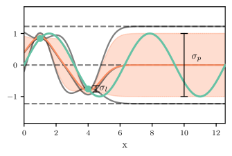
Figure 1: Illustration of an ensemble GPR model consisting of three models, the priors $p_{k}$ of the three models are depicted with dashed gray lines, each individual model is a full gray-line. The true function is green, and the mean prediction of the ensemble is orange with the shaded area being the model’s uncertainty.

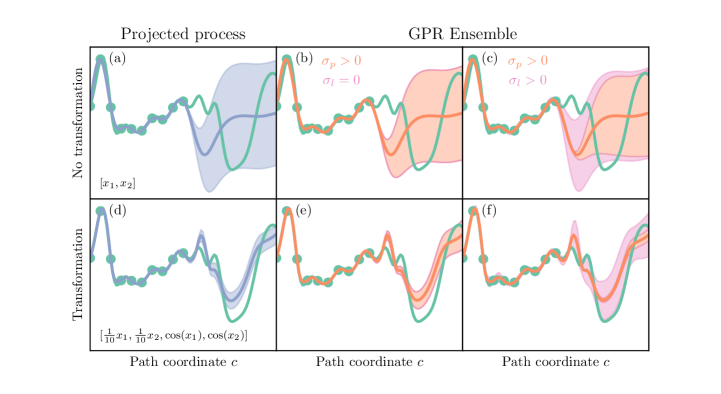
Figure 2: GP model fits of the function $f(x_{1},x_{2})=\cos(x_{1})+\frac{x_{2}\cos(x_{2})}{2}$, along a path. In the top row (a-c) the models use $(x_{1},x_{2})$ as features, whereas in the bottom row (d-f) $(\frac{1}{10}x_{1},\frac{1}{10}x_{2},\cos(x_{1}),\cos(x_{2}))$ is used as features exploiting the periodicity of the function to transform the feature space. In each row the model fit is the same for every model, the difference lies in the predicted uncertainty. Without a transformation of the feature all three models are very similar and the use of label noise $\sigma_{l}$ may seem unnecessary. However, once the transformation is introduced the longer length-scales that yield superior fits in the extrapolation region the label-noise uncertainty is qualitatively correct.

In figure 2 we show three different models, the projected-process sparse GPR, an ensemble GPR utilizing only the prior $\sigma_{p}$ noise to introduce an uncertainty, and a ensemble GPR utilizing both the prior $\sigma_{p}$ and label $\sigma_{l}$ noise. When fitting the potential energy surface descriptors that obey translational, rotational and permutational invariance are always used. These descriptors encode invariant properties such as bond lengths and angles, which correlate distinct atomic configuration. This correlation means that a model can and should have low predicted uncertainty about configurations that may naively appear to be far from any training example. We illustrate the effect of this on the three models in Figure 2(d-f), by choosing features that introduce a similar transformation of feature space. This means that for most kernel length-scales no point is particularly far from a training example and as such only a small fraction of $\sigma_{p}$ can ever be realized - whereas even a small $\sigma_{l}$ can lead to a significant uncertainty.

The form of Eq. (3) is advantageous as the training, where the majority of the computational expense is computing the matrix $C$, only needs to be done once, rather than for each constituent model. Similarly, for making predictions the kernel vector $\mathbf{k}_{m}(\mathbf{x})$ also only needs to be calculated once, meaning that predictions for every constituent model can be made at barely any extra computational cost.

II Calibration

In this section, we compare the quality of the uncertainty prediction made with the standard closed-form posterior uncertainty expression of a projected process (see section VI.1 for an introduction) with our proposed ensemble uncertainty method. The methodology of calibration curves and errors are presented in section VI.3

A dataset of Au_x with $x=[10,12,14,16,18,20]$ consisting of 5838 structures has been gathered by selecting structures with unique graphs Christiansen et al. (2022); Slavensky and Hammer (2024) from a set of global structure searches for each cluster size. This dataset is split into a training set, a validation set and a test set of 225, 25 and 5588 structures respectively. In Fig. 3 we show the parity plots for a subset of the test data and calibration plots for both models with optimized hyperparameters. Both models are capable of achieving good fits with the relatively small amount of training data and both produce well calibrated uncertainties.

For this comparison, we train on the training set and use the validation set to calibrate the uncertainties. This calibration amounts to finding hyperparameters. From the outset we choose the kernel form (see kernel definition in Eq. (7)) and its length-scale as $l=20$. Having fixed the length-scale, the regular sparse GPR has two hyperparameters that can influence the predicted uncertainties, namely the kernel amplitude $\theta_{0}$ and the noise $\sigma_{n}$. However, if these are chosen independently the model predictions are influenced, to avoid that, we fix the ratio $\frac{A}{\sigma_{n}}=100$. The calibration error can then be minimized wrt. these two parameters while keeping the ratio fixed.

For the ensemble model, we can freely minimize the calibration error wrt. to the two additional noise parameters of the ensemble $\sigma_{l}$ and $\sigma_{p}$, while fixing $\theta_{0}=1$ and $\sigma_{n}=0.01$ keeping the same ratio as for the regular sparse GPR.

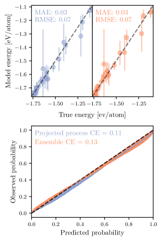
Figure 3: Top left and top right: parity plots with error-bars for the predicted uncertainty for a few randomly selected structures with the regular sparse GPR model and the ensemble model, respectively. MAE and RMSE for the full dataset are reported in eV/atom. Bottom: Calibration curves for ensemble and regular model in blue and orange, respectively. The values for the calibration error (CE) are given. For the ensemble model, Eq. (5) is used for the variance, while for the regular model, Eq. (11) is used.

III Global structure search

To probe the utility of this model we employ it in an active learning global structure search algorithm. In each iteration of the algorithm several structural candidates are stochastically generated and subsequently locally optimized in the lower-confidence-bound expression:

$$E_{\mathrm{LCB}}(X)=E(X)-\kappa\sigma(X),$$ (6)

where $E(X)$ is model total energy prediction, $\sigma(X)$ is the predicted standard deviation, and $\kappa$ is a hyperparameter balancing the importance of the uncertainty. Among these structural candidates the one with the lowest value of $E_{LCB}(X)$ is selected for evaluation with DFT and that structure is added to the training set of the model before moving on to the next iteration. The uncertainty therefore plays a large role in efficiently exploring the search space.

For the largest of the gold clusters, 20 atoms, studied in the previous section we run many independent searches. For each search we record how many iterations are required in order to find the global minimum structure, a perfect tetrahedron, as a function of the exploration parameter $\kappa$. If the uncertainty measure is suited for this task, there must exist a $\kappa\neq 0$ that increases the number of successful searches compared to searches with $\kappa=0$. In Figure 4 we present the success rate, that is the percentage of searches that find the GM structure, as a function of $\kappa$ for both the ensemble GPR and the regular GPR using the projected process expression for the uncertainty. For the ensemble there is a clear improvement in the search performance as $\kappa$ is increased – thus the uncertainty helps the algorithm explore the configuration space more efficiently.

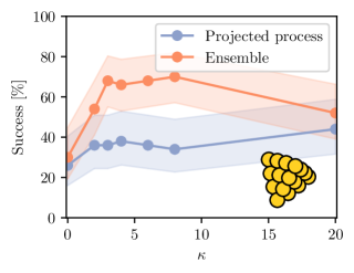
Figure 4: Success as a function of $\kappa$ for Au₂₀ for projected process and ensemble models.

IV Timings

The allure of machine learning models comes in large part from them being orders of magnitude faster than traditional quantum mechanical methods, such as DFT. Even so, for a task such as the global structure search described in the previous section, performing local optimizations in the model constitutes a significant fraction of the total time.

When making a prediction with either type of model the matrix vector of coefficients $\alpha=C\mathbf{E}$ can be precomputed for the current training set. For the ensemble model this means that the $\alpha$-vector for each model in the ensemble can be stored and the time spent calculating the uncertainty from Eq. (5) mainly involves calculating the kernel vectors $\mathbf{k}_{m}(x)$.

Figure 5 shows timings for training and prediction with both discussed types of models on configurations of Au₂₀ clusters. Here training covers computing $C\mathbf{E}$ in Eq. (1) and the required matrices for calculating uncertainties, such that predictions can be made as fast as possible. As a function of the number of training configurations with a fixed number of inducing points the sparsification procedure is the dominating part of the timings, with only a relatively small additional time for the projected-process model as it involves inverting additional matrices. With a fixed set of training data but a varying number of inducing points a more pronounced difference between the two methods can be observed, which again can be attributed to the projected-process uncertainty expression needing the construction and inversion of additional matrices that grow with the number of inducing points. Finally for predictions on 50 configurations, for the ensemble the timings are dominated by the pre-computing features and kernel elements between the query configuration and the set of inducing points. Whereas, for larger sets of inducing points the calculation of uncertainties and especially derivatives of the uncertainties in the projected process starts becoming a significant proportion of the time.

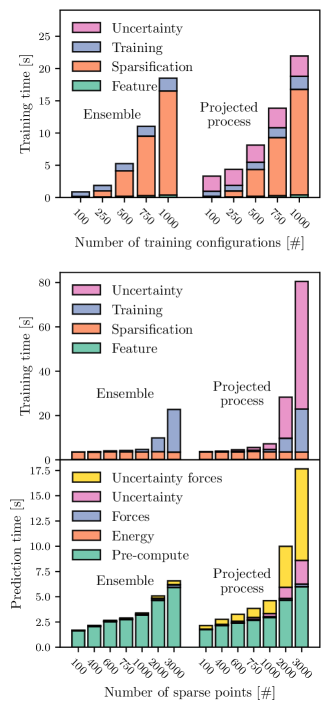
Figure 5: The top and middle panels show timings for different components of training each model and the bottom panel shows timings for making predictions with each model. Timings were done on Intel Xeon Gold 6230 CPUs and averaged over 10 separate runs.

V Disucssion

We have investigated the efficacy of two expressions for predicting uncertainties of GPR models in the realm of atomistic simulations. It has been shown that both models can produce well-calibrated uncertainties. However, in a common material science simulation task, namely global structure search for atomic configurations we have found that the proposed ensemble GPR uncertainty expression is advantageous. Further, we document that the ensemble method has superior behavior in terms of computational cost – both when it comes to training and prediction.

VI Methods

VI.1 Sparse Gaussian Process Regression

We have previously reported on a sparse local GPR Rønne et al. (2022), where the covariance between local enviroment descriptors is given by

$$k(\mathbf{x}_{i},\mathbf{x}_{j})=\theta_{0}\exp\left(-\frac{|\mathbf{x}_{i}-\mathbf{x}_{j}|^{2}}{2l^{2}}\right).$$ (7)

Here, $\theta_{0}$ and $l$ are amplitude and length-scale hyperparameters of this radial basis function kernel. With a training dataset $X_{n}$ and a set of inducing points $X_{m}$, we can define covariance matrices $K_{mm}$ and $K_{nm}$ as the covariance between all descriptors in $X_{m}$ and $X_{m}$ and $X_{n}$ and $X_{m}$. From that, we can define

$$C=\left[K_{mm}+(LK_{nm})^{T}\Sigma_{nn}^{-1}(LK_{nm})\right]^{-1}(LK_{nm})^{T}\Sigma^{-1},$$ (8)

where $\Sigma_{nn}$ is a diagonal matrix with the noise of each environment and a local energy may be predicted using

$$\epsilon(\mathbf{x})=\mathbf{k}_{m}(\mathbf{x})C\mathbf{E}.$$ (9)

Here $\mathbf{E}$ are the observed total energies and $L$ is a local energy correspondence matrix. Compared to a non-sparse GPR model, which is recovered in the limit where $X_{m}=X_{n}$, the sparse GPR comes at reduced computational cost as the matrix that is inverted is only of size $m\times m$ and the vector of kernel elements between a query-point and $X_{m}$ does not grow with the training set size. From an intuitive point of view this sparsification also necessitates a change to the predicted variance. In the projected process form the covariance is given by Rasmussen and Williams (2006):

$$\varsigma(\mathbf{x}_{i},\mathbf{x}_{j})^{2}=k(\mathbf{x}_{i},\mathbf{x}_{j})-\mathbf{k}^{T}_{m}(\mathbf{x}_{i})K_{mm}^{-1}\mathbf{k}_{m}(\mathbf{x}_{j})$$ (10)

$$+\mathbf{k}_{m}(\mathbf{x}_{i})^{T}(K_{mm}+K_{mn}\Sigma^{-1}_{nn}K_{nm})^{-1}\mathbf{k}_{m}(\mathbf{x}_{j}).$$

Here $\varsigma(\mathbf{x_{i}},\mathbf{x_{j}})^{2}$ is the predicted covariance of two local energies. As $\Sigma_{nn}$ involves every local environment in the training set it can become quite large, so unless a sparse matrix implementation is used that can lead to memory issues. Further, the matrix product involving $\Sigma_{nn}$ is also much faster using a sparse matrix implementation. For the acquisition function considered in this work we are interested in the standard deviation of the total energy

$$\sigma(X)=\sqrt{\sum_{\mathbf{x}_{i}\in X}\sum_{\mathbf{x}_{j}\in X}\varsigma(\mathbf{x}_{i},\mathbf{x}_{j})^{2}}$$ (11)

that takes into account the covariances of the local energies.

VI.2 CUR Sparsification

In order to choose the local environments in the set of inducing points $X_{m}$ we employ the CUR algorithm Mahoney and Drineas (2009). Here the full feature matrix $X_{n}$, that has dimensions $(n,f)$ where $n$ is the number of local environments and $f$ is the number of features, is decomposed by singular value decomposition into three matrices $X_{n}=U\Sigma V$, where $\Sigma$ is a diagonal matrix with entries in descending order. A probability of selection is then calculated for each local enviroment, indexed by $i$, as

$$P_{i}\propto\sum_{j<k}{U_{ij}^{2}}$$ (12)

where $k=\min(n,f)$ which for all but the smallest datasets is equal to $f$. A predetermined number $m$ of environments is finally picked, based on the calculated probabilities, in order to establish the set of inducing points $X_{m}$.

VI.3 Calibration

In the context of uncertainty quantification calibration refers to ensuring that the true labels fall within a certain confidence interval given by the predicted standard deviation. To this end we use calibration plots, as introduced by Kuleshov et al. (2018), to asses the quality of the uncertainty estimate of a given model. When recalibrating models we minimize their calibration error, also defined by Kuleshov et al. (2018). These metrics have been employed by other authors in the area of MLIPs Tran et al. (2020); Hu et al. (2022).

VII Code availability

The code used the findings presented in this paper is publicly available as part of AGOX as of version 2.7.0 at https://gitlab.com/agox/agox under a GNU GPLv3 license.

VIII Acknowledgements

We acknowledge support from VILLUM FONDEN through Investigator grant, project no. 16562, and by the Danish National Research Foundation through the Center of Excellence “InterCat” (Grant agreement no: DNRF150).

References

- Behler and Parrinello (2007) J. Behler and M. Parrinello, Phys. Rev. Lett. 98, 146401 (2007).
- Bartók et al. (2010) A. P. Bartók, M. C. Payne, R. Kondor, and G. Csányi, Phys. Rev. Lett. 104, 136403 (2010).
- Deringer and Csányi (2017) V. L. Deringer and G. Csányi, Phys. Rev. B 95, 094203 (2017).
- Deringer et al. (2021a) V. L. Deringer, N. Bernstein, G. Csányi, C. B. Mahmoud, M. Ceriotti, M. Wilson, D. A. Drabold, and S. R. Elliott, Nature 589, 59 (2021a).
- Vandermause et al. (2022) J. Vandermause, Y. Xie, J. S. Lim, C. J. Owen, and B. Kozinsky, Nature Communications 13, 5183 (2022).
- Gastegger et al. (2017) M. Gastegger, J. Behler, and P. Marquetand, Chem. Sci. 8, 6924 (2017).
- Tang et al. (2023) Z. Tang, S. T. Bromley, and B. Hammer, The Journal of Chemical Physics 158, 224108 (2023), https://pubs.aip.org/aip/jcp/article-pdf/doi/10.1063/5.0150379/17979772/224108_1_5.0150379.pdf .
- Kolsbjerg et al. (2018) E. L. Kolsbjerg, A. A. Peterson, and B. Hammer, Phys. Rev. B 97, 195424 (2018).
- Paleico and Behler (2020) M. L. Paleico and J. Behler, The Journal of Chemical Physics 153, 054704 (2020).
- Timmermann et al. (2020) J. Timmermann, F. Kraushofer, N. Resch, P. Li, Y. Wang, Z. Mao, M. Riva, Y. Lee, C. Staacke, M. Schmid, C. Scheurer, G. S. Parkinson, U. Diebold, and K. Reuter, Phys. Rev. Lett. 125, 206101 (2020).
- Wang et al. (2021) Y. Wang, L. Zhang, B. Xu, X. Wang, and H. Wang, Modelling Simul. Mater. Sci. Eng. 30, 025003 (2021).
- Timmermann et al. (2021) J. Timmermann, Y. Lee, C. G. Staacke, J. T. Margraf, C. Scheurer, and K. Reuter, The Journal of Chemical Physics 155, 244107 (2021).
- Merte et al. (2022) L. R. Merte, M. K. Bisbo, I. Sokolović, M. Setvín, B. Hagman, M. Shipilin, M. Schmid, U. Diebold, E. Lundgren, and B. Hammer, Angewandte Chemie International Edition 61, e202204244 (2022).
- Lee et al. (2023) Y. Lee, J. Timmermann, C. Panosetti, C. Scheurer, and K. Reuter, J. Phys. Chem. C 127, 17599 (2023).
- Ouyang et al. (2015) R. Ouyang, Y. Xie, and D.-e. Jiang, Nanoscale 7, 14817 (2015).
- Tong et al. (2018) Q. Tong, L. Xue, J. Lv, Y. Wang, and Y. Ma, Faraday Discuss. 211, 31 (2018).
- Arrigoni and Madsen (2021) M. Arrigoni and G. K. H. Madsen, npj Comput Mater 7, 1 (2021).
- Wang et al. (2023) J. Wang, H. Gao, Y. Han, C. Ding, S. Pan, Y. Wang, Q. Jia, H.-T. Wang, D. Xing, and J. Sun, National Science Review 10, nwad128 (2023).
- Valle and Oganov (2010) M. Valle and A. R. Oganov, Acta Crystallogr A Found Crystallogr 66, 507 (2010).
- Behler (2011) J. Behler, The Journal of Chemical Physics 134, 074106 (2011).
- Rupp et al. (2012) M. Rupp, A. Tkatchenko, K.-R. Müller, and O. A. Von Lilienfeld, Phys. Rev. Lett. 108, 058301 (2012).
- Bartók et al. (2013) A. P. Bartók, R. Kondor, and G. Csányi, Phys. Rev. B 87, 184115 (2013).
- Faber et al. (2018) F. A. Faber, A. S. Christensen, B. Huang, and O. A. von Lilienfeld, The Journal of Chemical Physics 148, 241717 (2018).
- Drautz (2019) R. Drautz, Phys. Rev. B 99, 014104 (2019).
- Huo and Rupp (2022) H. Huo and M. Rupp, Mach. Learn.: Sci. Technol. 3, 045017 (2022), arXiv:1704.06439 [cond-mat, physics:physics] .
- Gilmer et al. (2017) J. Gilmer, S. S. Schoenholz, P. F. Riley, O. Vinyals, and G. E. Dahl, “Neural Message Passing for Quantum Chemistry,” (2017), arXiv:1704.01212 [cs] .
- Schütt et al. (2017) K. T. Schütt, P.-J. Kindermans, H. E. Sauceda, S. Chmiela, A. Tkatchenko, and K.-R. Müller, “SchNet: A continuous-filter convolutional neural network for modeling quantum interactions,” (2017), arXiv:1706.08566 [physics, stat] .
- Xie and Grossman (2018) T. Xie and J. C. Grossman, Phys. Rev. Lett. 120, 145301 (2018).
- Gasteiger et al. (2019) J. Gasteiger, J. Groß, and S. Günnemann, in International Conference on Learning Representations (2019).
- Thomas et al. (2018) N. Thomas, T. Smidt, S. Kearnes, L. Yang, L. Li, K. Kohlhoff, and P. Riley, “Tensor field networks: Rotation- and translation-equivariant neural networks for 3D point clouds,” (2018), arXiv:1802.08219 [cs] .
- Anderson et al. (2019) B. Anderson, T.-S. Hy, and R. Kondor, “Cormorant: Covariant Molecular Neural Networks,” (2019), arXiv:1906.04015 [physics, stat] .
- Schütt et al. (2021) K. Schütt, O. Unke, and M. Gastegger, in Proceedings of the 38th International Conference on Machine Learning (PMLR, 2021) pp. 9377–9388.
- Batzner et al. (2022) S. Batzner, A. Musaelian, L. Sun, M. Geiger, J. P. Mailoa, M. Kornbluth, N. Molinari, T. E. Smidt, and B. Kozinsky, Nat Commun 13, 2453 (2022).
- Batatia et al. (2023) I. Batatia, D. P. Kovács, G. N. C. Simm, C. Ortner, and G. Csányi, “MACE: Higher Order Equivariant Message Passing Neural Networks for Fast and Accurate Force Fields,” (2023), arXiv:2206.07697 [cond-mat, physics:physics, stat] .
- Unke and Meuwly (2019) O. T. Unke and M. Meuwly, J. Chem. Theory Comput. 15, 3678 (2019).
- Behler and Csányi (2021) J. Behler and G. Csányi, Eur. Phys. J. B 94, 142 (2021).
- Anstine and Isayev (2023) D. M. Anstine and O. Isayev, J. Phys. Chem. A 127, 2417 (2023).
- Botu et al. (2017) V. Botu, R. Batra, J. Chapman, and R. Ramprasad, J. Phys. Chem. C 121, 511 (2017).
- A. Peterson et al. (2017) A. A. Peterson, R. Christensen, and A. Khorshidi, Physical Chemistry Chemical Physics 19, 10978 (2017).
- Tran et al. (2020) K. Tran, W. Neiswanger, J. Yoon, Q. Zhang, E. Xing, and Z. W. Ulissi, Mach. Learn.: Sci. Technol. 1, 025006 (2020), publisher: IOP Publishing.
- Wen and Tadmor (2020) M. Wen and E. B. Tadmor, npj Comput Mater 6, 1 (2020).
- Hu et al. (2022) Y. Hu, J. Musielewicz, Z. W. Ulissi, and A. J. Medford, Mach. Learn.: Sci. Technol. 3, 045028 (2022), publisher: IOP Publishing.
- Rasmussen et al. (2023) M. H. Rasmussen, C. Duan, H. J. Kulik, and J. H. Jensen, Journal of Cheminformatics 15, 121 (2023).
- Carrete et al. (2023) J. Carrete, H. Montes-Campos, R. Wanzenböck, E. Heid, and G. K. H. Madsen, The Journal of Chemical Physics 158, 204801 (2023).
- Jørgensen et al. (2023) P. B. Jørgensen, J. Busk, O. Winther, and M. N. Schmidt, “Coherent energy and force uncertainty in deep learning force fields,” (2023), arXiv:2312.04174 [physics, stat] .
- Zhu et al. (2023) A. Zhu, S. Batzner, A. Musaelian, and B. Kozinsky, The Journal of Chemical Physics 158, 164111 (2023).
- Tan et al. (2023) A. R. Tan, S. Urata, S. Goldman, J. C. B. Dietschreit, and R. Gómez-Bombarelli, npj Comput Mater 9, 1 (2023).
- Behler (2015) J. Behler, International Journal of Quantum Chemistry 115, 1032 (2015).
- Zaverkin et al. (2022) V. Zaverkin, D. Holzmüller, I. Steinwart, and J. Kästner, Digital Discovery 1, 605 (2022).
- van der Oord et al. (2023) C. van der Oord, M. Sachs, D. P. Kovács, C. Ortner, and G. Csányi, npj Comput Mater 9, 1 (2023).
- Kulichenko et al. (2023) M. Kulichenko, K. Barros, N. Lubbers, Y. W. Li, R. Messerly, S. Tretiak, J. S. Smith, and B. Nebgen, Nat Comput Sci 3, 230 (2023).
- Zaverkin et al. (2024) V. Zaverkin, D. Holzmüller, H. Christiansen, F. Errica, F. Alesiani, M. Takamoto, M. Niepert, and J. Kästner, npj Comput Mater 10, 1 (2024).
- Hernández-Lobato et al. (2017) J. M. Hernández-Lobato, J. Requeima, E. O. Pyzer-Knapp, and A. Aspuru-Guzik, in Proceedings of the 34th International Conference on Machine Learning (PMLR, 2017) pp. 1470–1479.
- Todorović et al. (2019) M. Todorović, M. U. Gutmann, J. Corander, and P. Rinke, Npj computational materials 5, 35 (2019).
- Bisbo and Hammer (2020) M. K. Bisbo and B. Hammer, Phys. Rev. Lett. 124, 086102 (2020).
- Kaappa et al. (2021) S. Kaappa, E. G. Del Río, and K. W. Jacobsen, Phys. Rev. B 103, 174114 (2021).
- Schran et al. (2020) C. Schran, K. Brezina, and O. Marsalek, The Journal of Chemical Physics 153, 104105 (2020).
- Montes-Campos et al. (2022) H. Montes-Campos, J. Carrete, S. Bichelmaier, L. M. Varela, and G. K. H. Madsen, J. Chem. Inf. Model. 62, 88 (2022).
- Kahle and Zipoli (2022) L. Kahle and F. Zipoli, Phys. Rev. E 105, 015311 (2022).
- Busk et al. (2023) J. Busk, M. N. Schmidt, O. Winther, T. Vegge, and P. B. Jørgensen, “Graph Neural Network Interatomic Potential Ensembles with Calibrated Aleatoric and Epistemic Uncertainty on Energy and Forces,” (2023), arXiv:2305.16325 [physics] .
- Deringer et al. (2021b) V. L. Deringer, A. P. Bartók, N. Bernstein, D. M. Wilkins, M. Ceriotti, and G. Csányi, Chem. Rev. 121, 10073 (2021b).
- Hüllermeier and Waegeman (2021) E. Hüllermeier and W. Waegeman, Mach Learn 110, 457 (2021).
- Christiansen et al. (2022) M.-P. V. Christiansen, N. Rønne, and B. Hammer, The Journal of Chemical Physics 157, 054701 (2022).
- Slavensky and Hammer (2024) A. M. Slavensky and B. Hammer, The Journal of Chemical Physics 161, 014713 (2024).
- Rønne et al. (2022) N. Rønne, M.-P. V. Christiansen, A. M. Slavensky, Z. Tang, F. Brix, M. E. Pedersen, M. K. Bisbo, and B. Hammer, The Journal of Chemical Physics 157, 174115 (2022).
- Rasmussen and Williams (2006) C. E. Rasmussen and C. K. I. Williams, Gaussian Processes for Machine Learning, Adaptive Computation and Machine Learning (MIT Press, Cambridge, Mass, 2006).
- Mahoney and Drineas (2009) M. W. Mahoney and P. Drineas, Proc. Natl. Acad. Sci. U.S.A. 106, 697 (2009).
- Kuleshov et al. (2018) V. Kuleshov, N. Fenner, and S. Ermon, in Proceedings of the 35th International Conference on Machine Learning (PMLR, 2018) pp. 2796–2804, iSSN: 2640-3498.