Global bifurcations organizing weak chimeras in three symmetrically coupled Kuramoto oscillators with inertia
Abstract
Frequency desynchronized attractors cannot appear in identically coupled symmetric phase oscillators because “overtaking” of phases cannot occur. This restriction no longer applies for more general identically coupled oscillators. Hence, it is interesting to understand precisely how frequency synchrony is lost and how invariant sets such as attracting weak chimeras are generated at torus breakup, where the phase description breaks down. Maistrenko et al (2016) found numerical evidence of an organizing center for weak chimeras in a system of coupled identical Kuramoto oscillators with inertia. This paper identifies this organizing center and shows that it corresponds to a particular type of non-transverse heteroclinic bifurcation that is generic in the context of symmetry. At this codimension two bifurcation there is a splitting of connecting orbits between the in-phase (fully synchronized) state. This generates a wide variety of associated bifurcations to weak chimeras. We further highlight a second organizing center associated with a codimension two symmetry-breaking heteroclinic connection.
1 Introduction
Coupled oscillators are of great interest for a variety of applications where they provide tractable models of spatio-temporal pattern generation through interaction between systems with attracting periodic behavior. For weak coupling of hyperbolic attracting limit cycle oscillators, a standard normal hyperbolicity argument [1] means there is an attracting invariant -torus containing all nearby attractors. For a general system of non-identical oscillators and in this limit of weak coupling bifurcations a wide variety of partial frequency synchronized solutions were found in [2]. These involved considering perturbations of the intrinsic frequencies of the oscillators. It is natural to ask whether these frequency-desynchronized solutions can appear spontaneously, rather than through forced symmetry breaking.
The general case of symmetrically coupled phase oscillators was considered for example in [3, 4, 5]. A result from [3] is that for such systems with full permutation symmetry , the low dimensionality means that only frequency synchronized solutions can appear, even though a wide variety of phase dynamics are possible.
The possibility of breaking of frequency synchrony in networks of oscillators that are still identical is discussed in [6] where the idea of a weak chimera as a symmetry breaking of frequencies is introduced. It is also highlighted in [6] that because of the presence of 2-in-phase invariant subspaces that are codimension one in the phase space of phase differences, weak chimeras cannot appear in -symmetric phase oscillators. But they can appear in a wide range of less symmetric networks that still have a transitive action of symmetries which mean all oscillators can be viewed as identical. For example, they can be found in oscillator networks with modular structures [6] or rings with next-nearest neighbor coupling [7]. Similar structures can be found that relate chaotic dynamics [8, 9].
Such solutions with broken frequency symmetry can also occur for more general -symmetric fully symmetric coupled oscillators: For example, chimeras can be found in coupled Landau oscillators with full permutation symmetry [10]. This leads to the interesting question of how the breakdown of an invariant -torus associated with weak coupling can lead to the appearance of solutions with broken frequency synchrony. The smallest case where one could plausibly see this is for three fully and identically coupled phase oscillators with symmetry. Indeed, this has been observed in 3 coupled Kuramoto-style oscillators with inertia [11], where a wide variety of periodic and chaotic solutions are found in the case that the damping is not too strong. Kuramoto oscillators with inertia have been used to model power grid networks [12] and show a range of dynamics [13]. For strong enough damping this reduces to Kuramoto oscillators with identical frequencies where neither chaos nor breaking of frequency synchrony is possible [3].
In this paper, we exhibit some bifurcations associated with heteroclinic networks that organize the emergence of frequency-synchronized solutions in three coupled Kuramoto oscillators with inertia. Firstly, we clarify the bifurcation happening at the organizing center identified in [11] and named in that work as Point B: By developing a bespoke Lin’s method [14, 15], we show numerically that this is a symmetric codimension-two homoclinic bifurcation where there is a tangency of stable and unstable manifolds. Specifically, we (a) find the space of bounded solutions of the variational equations and (b) set up a bifurcation function that is zero precisely when there is a tangency of manifolds. Numerical bifurcation analysis further sheds light on codimension-one bifurcations related to Point B. Secondly, we identify a further codimension-two Point C that corresponds to the existence of a heteroclinic connection between synchrony and a nontrivial equilibrium. This yields an entire network of heteroclinic connections that allow for complicated patterns of oscillator phases passing one another. These organizing centers are not only interesting examples of global bifurcations in symmetric systems in their own right but also elucidate how heteroclinic networks can lead to the emergence of weak chimeras in minimal networks of phase oscillators with inertia.
The rest of the paper is organized as follows: Section 2 introduces the model of three symmetric Kuramoto oscillators with inertia, and summarizes basic properties of the phase space. In Section 3, we discuss the equilibria of the system, their linear stability, and relevant bifurcations that are relevant for the codimension-two Point B. Section 4 identifies the bifurcation at Point B as a symmetric homoclinic tangency and confirms this numerically using Lin’s method. We turn to the global dynamics in parameter space near Point B in Section 5 and identify the codimension-two Point C as an organizing center. This point corresponds to a heteroclinic connection between distinct equilibria. We conclude with some remarks in Section 6.
2 Three globally coupled Kuramoto oscillators with inertia
In this paper, we analyze the dynamics and bifurcations of globally and identically coupled Kuramoto oscillators with inertia as in [11]. Specifically, the phase of oscillator evolves according to
| (1) |
for parameters , , , and . The system has a continuous phase-shift symmetry for . Without loss of generality, we may assume by exploiting the phase shift symmetry and set by rescaling and . Note that rescaling time with corresponds to a parameter transformation . We henceforth fix as in [11].
Due to the global and identical coupling, the system (1) is equivariant with respect to the symmetric group of three elements acting by permuting the indices of the oscillators. The symmetry implies the existence of invariant sets
| (2) |
which correspond to phase configurations where two oscillators are synchronized in phase and frequency. Note that is generated by the three cycle and the transposition ; observe that permutes the invariant sets (2) while permutes and and leaves invariant. The invariant sets intersect in the in-phase solution
| (3) |
2.1 Phase-difference coordinates
As in [11] we introduce phase-difference coordinates , to reduce the phase-shift symmetry. In these coordinates and setting , the system (1) reduces to
| (4a) | ||||
| (4b) | ||||
that determines the evolution of . Writing and , (4) is equivalent to
| (5a) | ||||
| (5b) | ||||
| (5c) | ||||
| (5d) | ||||
In the phase-difference coordinates, the invariant subspaces are given by
| (6) |
as illustrated in Figure 1(a). The action of the generators of is given by and .
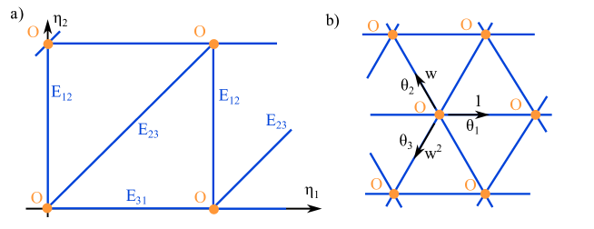
2.2 Symmetric coordinates
A coordinate system where permutations of the oscillators act orthogonally is given by a complex phase
| (7) |
where ; see also [3]. These coordinates also reduce the phase-shift symmetry since is invariant with respect to it. In the complex phase coordinates we have
| (8) |
as illustrated in Figure 1(b). Now acts by multiplication with . Note that phase-difference coordinates and the complex phase variables are related through
| (9) |
3 Equilibria and bifurcations
We first give an overview of the equilibria and their stability, and identify the essential bifurcations that organize the dynamics. In Section 5 we complement the results given in [11] by numerical continuation analysis in Auto [16] and by numerical exploration.
Up to symmetry, we classify two equilibria. First, the in-phase solution at the origin is an equilibrium in reduced coordinates. Second, there is one nontrivial equilibrium in each invariant subspace : The subspace contains the equilibrium with
independent of and . Its symmetric copies in and are and , respectively. In the covering space of the phase space , we write
| (10) | ||||
| (11) |
denote the equilibria and their symmetric counterparts. We omit the indices of the specific subspaces or equilibria and just write , , or unless the context means the indices are relevant.
3.1 Linear stability
The structure of the equations of motion and the symmetries restrict the stability properties of the vector field. Let denote the vector field of the system of first-order ODEs corresponding to (4). The linearization of at a point is
| (12) |
If denote the eigenvalues of , we have
| (13) |
For points on the invariant subspaces two eigenvalues correspond to eigenvectors that are parallel to and two that are transverse; we denote them by and , respectively. Restricting to the invariant subspaces we have that and thus
| (14) |
These conditions hold in particular for the linearization at the equilibria and (corresponding to limit cycles in the original system) and restrict their eigenvalues. If with is an eigenvalue then (14) implies that . For the equilibrium , symmetry implies .
3.2 Dynamics and bifurcations of cluster states
For the equilibrium is a stable bifocus. For the equilibria and undergo a (symmetric) transcritical bifurcation (TC). Henceforth we primarily focus on beyond the transcritical bifurcation point. In terms of notation, for equilibria , we write for a homoclinic connection from to ; heteroclinic connections are denoted with and indicates that the connection lies in .

We first restrict our attention to the dynamics within the invariant (cluster) space . For a fixed and varying phase lag (indicated by a dashed line in Figure 2). The saddle and sink have a codimension zero connection in . A branch of periodic orbits corresponds to partially synchronized weak chimera dynamics: Two oscillators are phase-synchronized and rotate relative to the remaining oscillator. As is decreased, continuation of this branch of periodic orbits leads to a homoclinic bifurcation involving a homoclinic orbit at as is decreased (red line in Figure 2). As is increased, the periodic orbit bifurcates in a homoclinic bifurcation involving at (orange line in Figure 2).
Between the red and orange lines shown in Figure 2 there is a limit cycle within . The existence of this periodic solution is bounded by the homoclinic bifurcation branches and . Continued in two parameters, these branches come together on the transcritical bifurcation line—marked as Point A in Figure 2.
3.3 Solutions breaking cluster states
Further bifurcations lead to stable dynamics off the invariant set where the oscillators form clusters. Continuation in one parameter with fixed shows that the branch of periodic orbits in considered above loses stability in a pitchfork bifurcation of limit cycles (PFoLC) at (green line in Figure 2). This results in two symmetry-related branches of a stable limit cycle with partial frequency synchrony off (but broken phase-synchrony111This transition from a phase- and frequency synchronized weak chimera solution to a solution that synchronized in frequency but not in phase is referred in [11] to “the chimeras becoming imperfect”.). These branches lose stability in a period-doubling bifurcation PD1 (blue line in Figure 2). Further bifurcations of the periodic orbits involve homoclinic orbits and that do not lie in (not shown in Figure 2).
The numerical continuation of these bifurcations in two parameters highlights a codimension-two point that organizes the emergence of these bifurcations between these phase-/frequency-synchrony patterns. As shown in Figure 2, the PFoLC and PD1 bifurcation curves continued in terminate on the point on the homoclinic bifurcation curve . This codimension-two point was already observed in [11] and dubbed Point B. It relates the bifurcations of weak chimera solutions on and off .
Indeed, for , the attracting dynamics are typically away from . This is captured by the quantity
| (15) |
that vanishes for . Thus, the average of will converge to zero for attractors that lie in while it will be nonzero otherwise. Note that the dynamics off may be chaotic as the invariant subspace is two-dimensional. Figure 2 shows averaged over trajectories for varying parameters together with bifurcation curves computed in Auto, illustrating some of the fine structure of the dynamics near Point B.
4 Bifurcations of the heteroclinic connection at Point B
We now consider the bifurcation occurring at Point B in more detail. We demonstrate that this is a symmetric homoclinic tangency bifurcation of the homoclinic connection; see [15] for general theory. To ease notation we write instead of the specific in the covering space unless necessary.
4.1 A codimension two symmetric homoclinic tangency bifurcation
First, note that in a large neighbourhood of Point B, the Jacobian (12) of (5) near the equilibrium has two identical real positive eigenvalues and two identical real negative eigenvalues. If denotes the stable manifold and the unstable manifold defined in the usual way, we have
i.e., both are two-dimensional invariant manifolds within . To find homoclinic connections we focus on a Poincaré section perpendicular to one of the invariant subspaces in . For concreteness, we consider the section
perpendicular to . Note that is the fixed point subspace of that acts on the reduced phase difference coordinates by
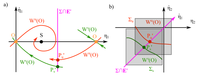
Restricted to , the section corresponds to a line; cf. Figure 3(a). Both the unstable manifold and the stable manifold will intersect in a single point, say and , respectively. Hence, it is generically codimension one that there are homoclinic connection from within if 222It is also generically codimension one that there can be connections that are not within ..
Now consider the full (reduced four-dimensional) phase space at . The tangent space at can be decomposed as
| (16) |
where , and . Given that and are both two-dimensional, it might be expected in a generic situation that
| (17) |
will only appear at codimension three in parameter space: and close to are line segments and it generically takes a two parameter variation to align them.
Here the problem is restricted by symmetry so that a tangency only requires varying one additional parameter leading to a codimension two homoclinic tangency. More specifically, note that since —and in particular —is fixed under we have that and close to into itself. This can only happen if , ; this is illustrated in Figure 3(b). This symmetry-induced constraint reduces the codimension by one allowing for a homoclinic tangency at codimension two.
4.2 A Lin’s method to find point B
We now develop a procedure based on Lin’s method [14] to determine the bifurcation point by finding and analysing the connecting orbit; see also [15]. The first step is to find the homoclinic orbit from to in , that is,
For the Jacobian let denote the left eigenvectors corresponding to the positive eigenvalues and the left eigenvectors corresponding to the negative eigenvalues. The problem can be expressed as a three-point boundary value problem on for large with four projection boundary conditions and one phase condition. Specifically, is a solution to the boundary value problem
| (18a) | ||||
| (18b) | ||||
| (18c) | ||||
| (18d) | ||||
| (18e) | ||||
| (18f) | ||||
We consider but work within the invariant subspace and so we only need to solve for the first two components. The , denote the stable and unstable subspaces, respectively, the middle four conditions of (18) are equivalent to
while the final equation in (18) is equivalent to the condition
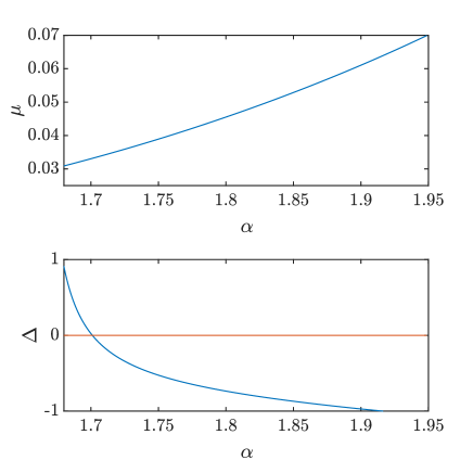
The system (18) is overdetermined, but fixing and allowing to vary will approximate the codimension one condition for the homoclinic orbit. This yields the curve of parameter values shown in (4) of parameter values where a homoclinic connection exists in ; this curve is identical to the orange curve in Figure 2 computed using Auto.
The second step is to determine any tangencies of the invariant manifolds. Note that in (16)—that aligns with the homoclinic connection—can be interpreted as the set of solutions of the variational equation that remain bounded as . Thus, in addition to (18) we consider solutions of the variational equation for 18 given by
| (19a) | ||||
| (19b) | ||||
| (19c) | ||||
| (19d) | ||||
| (19e) | ||||
| (19f) | ||||
| (19g) | ||||
More precisely, we need to find values of that satisfy (18) and where additionally the variational equations have two independent solutions.
We solve this problem using a Lin-type method by allowing solutions within to have a discontinuity in two of the components at . More precisely, we examine solutions of the six-dimensional boundary value problem (18),(19) in for large where all components of are continuous at except for the “gaps”
| (20a) | ||||
| (20b) | ||||
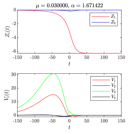
where , denote the limits to from the positive and negative side, respectively. Note that since is the only bounded solution of the variational equations that lies within the tangent space to but the final condition on (19) ensures that we are finding a nontrivial solution transverse to . We examine
and zeros of this correspond to homoclinic bifurcations that satisfy (17). This is illustrated in Figure 4 where we illustrate the where the homoclinic, the size of the gap along this curve and a typical solution for the Lin problem. Note that there is a unique location where corresponding to B. At this point note that also because of the symmetry .
5 Global dynamics, organizing centers, and Point C
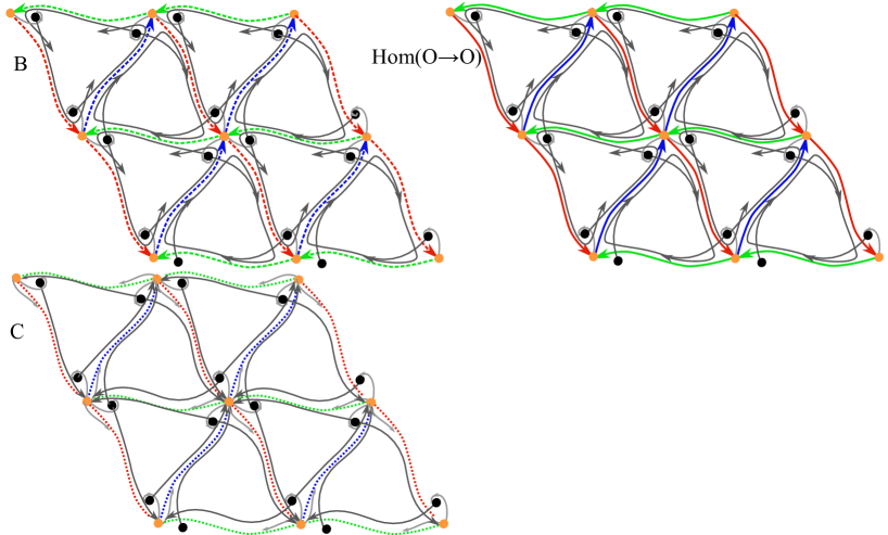
Varying parameters around Point B shows a wide range of dynamical behavior ranging from periodic to chaotic. We now show that these dynamics are organized by the interplay of the invariant manifolds of not only but also the nontrivial equilibria that can form heteroclinic connections and networks. Possibilities are sketched in Figure 5. On the one hand, these include not only the codimension-one homoclinic connection in as well as the additional codimension-two tangency at Point B discussed above. On the other hand, we find that there is an additional codimension-two Point C at which there is a heteroclinic connection off , which also organizes global dynamics.
5.1 Heteroclinic networks and chaotic dynamics
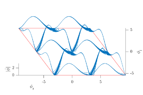
The chaotic attractors that appear close to Point B are characterized by phase slips associated with chimera states with rapid transitions along the sets . Figure 6 shows a single numerically approximated trajectory started close to that explored the unstable manifold of and hence also the unstable manifolds of in various copies on the torus. Note that trajectories repeatedly approach before being ejected along its one-dimensional unstable manifold. The chaotic dynamics near Point B appear to be organized by the interplay of the invariant manifolds of both and . Figure 5 illustrates the different heteroclinic connections that are possible: The codimension-zero connections are shown in purple and the codimension-one connections in , , are shown in red, green, and blue, respectively (so colors correspond to phase slips of one of the three oscillators). Moreover, the one-dimensional unstable manifold of (gray line in Figure 5) approaches and in a complicated sequential manner.

To gain insights into how the unstable manifold of wraps around the torus, we follow the sequence of “phase slips” along the transition—an increase of phase by an integer multiple of along one of the invariant subspaces . Our approach to visualize the winding of trajectories is inspired by the extraction of kneading sequences from the Lorentz equations in [17]. More precisely, we assign the connection in each a different color (as illustrated in Figure 5). Colors are then added in the sequence of the phase slips along each of the invariant subspaces with a weight that decays according to a geometric sequence: If follows a single this results in either red, blue, or green; transitions in the blue and then red direction give purple (with a shift towards red/blue depending on the order). More details on the algorithm are given in Appendix A.
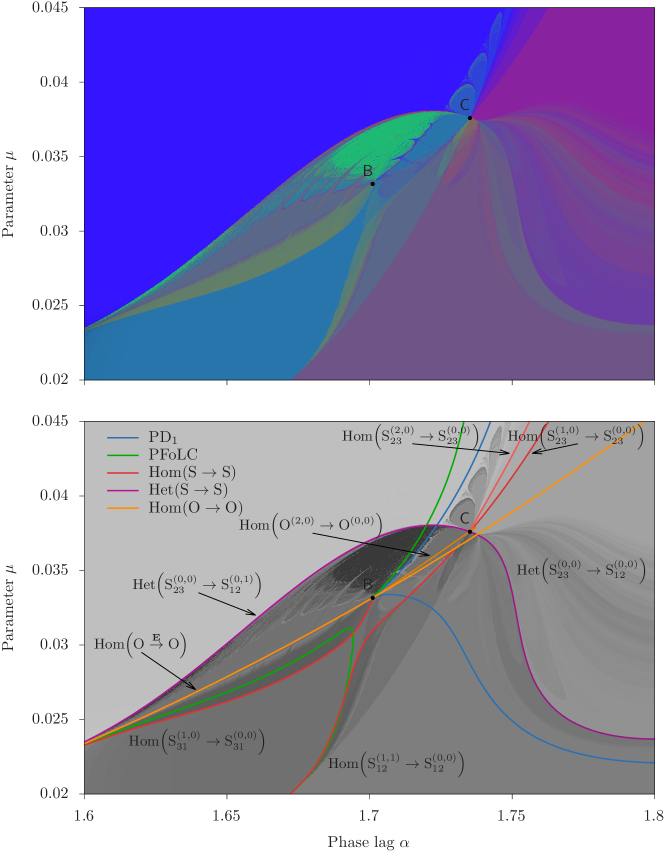
The sequences show the fine structure of the dynamics in parameter space as shown in Figure 7. Distinct colors can be found in the vicinity of Point B but the picture also unveils a rich structure. Further numerical bifurcation analysis (beyond what is shown in Figure 2) shows relevant (local and global) bifurcations that lead to qualitative changes in the phase slip sequences; see Figure 7(b). While Point B is related to the bifurcation lines shown in Figure 2, there is another codimension-two Point C that organizes the dynamics and bifurcations. Inspecting solutions along the bifurcation branches close to Point C shows that part of the heteroclinic connection off approaches a heteroclinic connection.
5.2 Heteroclinic connections at Point C
Heteroclinic connections are co-dimension two: Since the unstable manifold , it generically intersects a three-dimensional Poincaré section in a single point (cf. Figure 3). Variation of two parameters is required for this point to intersect the line that corresponds to the stable manifold of . Note that symmetry forces also heteroclinic connections of the symmetric copies. Solving the corresponding boundary value problem using XPP confirms the existence of an heteroclinic at in agreement of Point C identified in the previous section.
Note that the connection immediately gives rise to an entire heteroclinic network involving both and all symmetric copies of . Specifically, the codimension-zero connections within together with the off yields a heteroclinic connection . This means that there are pseudo-orbits that pass by and any symmetric copy of arbitrarily often. This facilitates the emergence of complicated phase-slip dynamics for parameter values near Point C.
6 Discussion
We show how certain homoclinic and heteroclinic structures and their bifurcations organize the dynamics in networks of three symmetrically coupled phase oscillators. First, we clarified the nature of the codimension-two organizing center corresponding to Point B in the paper of [11]: We find that Point B is a novel form of symmetric homoclinic tangency bifurcation that can be characterized only using connections between copies of the fully synchronized phase configuration . The bifurcation will only appear at this relatively low codimension because the presence of the symmetries forces the three invariant subspaces to coincide at . While it was somewhat a surprise that an analysis of connections to and from was not necessary to identify the organizing center first described in [11], we identified a second codimension-two Point C that does involve . The bifurcation at Point C is easier to identify as it corresponds to a connection between a one-dimensional unstable manifold of and the two-dimensional manifold of .
It will be a challenging problem for the future to unfold these bifurcations and to understand the wide variety of behaviors that can be observed to emerge from the organizing centers; cf. Figure 7. However, a main challenge to do this can be seen in Figure 5: A variety of symmetrically related sections will need to be chosen to ensure that trajectories leaving and are matched appropriately. Moreover, the fact that has two-dimensional unstable manifold near B means that potentially a large number of connections can be involved, including potentially some that connect for as indicated by numerical continuation (cf. Figure 7). We also expect to find heteroclinic orbits connecting equilibria and periodic orbits that can be continued with an appropriate boundary value setup [18, 19].
Together, the codimension-two points identified in this paper organize a wide variety of solutions—many of which partially break frequency synchrony—in its neighborhood. As previously noted, these cannot appear if there is an attracting invariant torus and so they are also indicative of crossing the threshold of torus breakdown. These organizing centers also point towards interesting phenomena of higher codimension: For example, at codimension three one would expect the existence of a heteroclinic network consisting of (codimension two), (codimension one), and (codimension zero) connections.
The bifurcations described can presumably be generalized to understand similar organizing centers for systems with larger , as illustrated in the numerical simulations of [11]. We have not attempted this but note that the dimensions of the Lin modeling of the variational equation will need to increase correspondingly.
Acknowledgments
Thanks to Yuri Maistrenko for suggesting that Point B was worthy of study. For the purpose of open access, the authors have applied a Creative Commons Attribution (CC–BY) license to any Author Accepted Manuscript version arising from this submission.
References
- [1] Frank C Hoppensteadt and Eugene M Izhikevich. Weakly connected neural networks, volume 126. Springer Science & Business Media, 2012.
- [2] Claude Baesens, John M. Guckenheimer, S. Kim, and Robert S. MacKay. Three coupled oscillators: mode-locking, global bifurcations and toroidal chaos. Physica D, 49(3):387–475, 1991.
- [3] Peter Ashwin, G P King, and James W. Swift. Three identical oscillators with symmetric coupling. Nonlinearity, 3(3):585–601, 1990.
- [4] Peter Ashwin, Oleksandr Burylko, and Yuri L. Maistrenko. Bifurcation to heteroclinic cycles and sensitivity in three and four coupled phase oscillators. Physica D, 237(4):454–466, 2008.
- [5] Peter Ashwin, Christian Bick, and Oleksandr Burylko. Identical Phase Oscillator Networks: Bifurcations, Symmetry and Reversibility for Generalized Coupling. Frontiers in Applied Mathematics and Statistics, 2(7):1–16, 2016.
- [6] Peter Ashwin and Oleksandr Burylko. Weak chimeras in minimal networks of coupled phase oscillators. Chaos, 25:013106, 2015.
- [7] Mary Thoubaan and Peter Ashwin. Existence and stability of chimera states in a minimal system of phase oscillators. Chaos: An Interdisciplinary Journal of Nonlinear Science, 28(10), 2018.
- [8] Christian Bick and Peter Ashwin. Chaotic weak chimeras and their persistence in coupled populations of phase oscillators. Nonlinearity, 29(5):1468, 2016.
- [9] Christian Bick. Isotropy of Angular Frequencies and Weak Chimeras with Broken Symmetry. Journal of Nonlinear Science, 27(2):605–626, 2017.
- [10] Gautam C Sethia and Abhijit Sen. Chimera states: The existence criteria revisited. Physical review letters, 112(14):144101, 2014.
- [11] Yuri L. Maistrenko, Serhiy Brezetsky, Patrycja Jaros, Roman Levchenko, and Tomasz Kapitaniak. Smallest chimera states. Physical Review E, 95(1):010203, 2017.
- [12] G. Filatrella, A. H. Nielsen, and N. F. Pedersen. Analysis of a power grid using a Kuramoto-like model. The European Physical Journal B, 61(4):485–491, 2008.
- [13] Simona Olmi, Erik A. Martens, Shashi Thutupalli, and Alessandro Torcini. Intermittent chaotic chimeras for coupled rotators. Physical Review E, 92(3):030901, 2015.
- [14] Xiao-Biao Lin. Using Melnikov’s method to solve Silnikov’s problems. Proceedings of the Royal Society of Edinburgh: Section A Mathematics, 116(3–4):295–325, 1990.
- [15] Ale Jan Homburg and Björn Sandstede. Homoclinic and heteroclinic bifurcations of vector fields. In Henk W. Broer, Takens Floris, and Boris Hasselblatt, editors, Handbook of Dynamical Systems Vol. 3, chapter 8, pages 379–524. Elsevier, 2010.
- [16] Eusebius J. Doedel, Randy C. Paffenroth, Alan R. Champneys, Thomas F. Fairgrieve, Yuri A. Kuznetsov, Bart E. Oldeman, Björn Sandstede, and Xianjun J. Wang. AUTO2000: Software for Continuation and Bifurcation Problems in Ordinary Differential Equations. Technical report, California Institute of Technology, Pasadena, CA, 2000.
- [17] Roberto Barrio, Andrey L. Shilnikov, and Leonid P. Shilnikov. Kneadings, Symbolic Dynamics and Painting Lorenz Chaos. International Journal of Bifurcation and Chaos, 22(04):1230016, apr 2012.
- [18] Bernd Krauskopf and Thorsten Rieß. A Lin’s method approach to finding and continuing heteroclinic connections involving periodic orbits. Nonlinearity, 21(8):1655–1690, 2008.
- [19] Eusebius J. Doedel, B. W. Kooi, G. A.K. Van Voorn, and Yuri A. Kuznetsov. Continuation of connecting orbits in 3D-ODEs: (I) point-to-cycle connections. International Journal of Bifurcation and Chaos, 18(7):1889–1903, 2008.
Appendix A Phase-Slip Sequences
We extract phase slips of either (along ), (along ), or both and simultaneously (along ) from the unstable manifold of is one-dimensional close to B. Note that—compared to evaluating the average frequencies—this strategy captures the transient as well as some indication of the asymptotic dynamics. For each parameter we execute the following steps:
-
1.
Choose an initial condition along the fastest expanding direction of : Let denote the eigenvalues of the linearization of the vector field at . Suppose that is an eigenvalue with corresponding eigenvector such that for all . For given , choose as initial condition.
-
2.
Solve the system for time units.
-
3.
Find times such that has a local extremum at that exceeds .
-
4.
For each determine
(21a) (21b) (21c) These coefficients correspond to an ‘orientation’ on .
-
5.
For given , evaluate
(22)
The sequences encoded by can be visualized by choosing three linearly independent color vectors (corresponding to red, green, and blue, for example) by plotting the (appropriately normalized) linear combination ; cf. Figure 7.