Individualized Federated Learning for Traffic Prediction with Error Driven Aggregation
Abstract
Low-latency traffic prediction is vital for smart city traffic management. Federated Learning has emerged as a promising technique for Traffic Prediction (FLTP), offering several advantages such as privacy preservation, reduced communication overhead, improved prediction accuracy, and enhanced adaptability to changing traffic conditions. However, majority of the current FLTP frameworks lack a real-time model updating scheme, which hinders their ability to continuously incorporate new incoming traffic data and adapt effectively to the changing dynamics of traffic trends. Another concern with the existing FLTP frameworks is their reliance on the conventional FL model aggregation method, which involves assigning an identical model (i.e., the global model) to all traffic monitoring devices to predict their individual local traffic trends, thereby neglecting the non-IID characteristics of traffic data collected in different locations. Building upon these findings and harnessing insights from reinforcement learning, we propose NeighborFL, an individualized real-time federated learning scheme that introduces a haversine distance-based and error-driven, personalized local models grouping heuristic from the perspective of each individual traffic node. This approach allows NeighborFL to create location-aware and tailored prediction models for each client while fostering collaborative learning. Simulations demonstrate the effectiveness of NeighborFL, offering improved real-time prediction accuracy over three baseline models, with one experimental setting showing a 16.9% reduction in MSE value compared to a naive FL setting.
Index Terms:
individualized federated learning, real-time traffic prediction, error-driven aggregation, distance heuristic, reinforcement learning, recurrent neural network.I Introduction
In the pursuit of high fidelity Traffic Prediction (TP), Federated Learning (FL) has emerged as a technique with promising performance in traffic flow prediction [1] and speed prediction [2]. Compared to the conventional centralized approach [3], FL presents a myriad of advantages that contribute to its growing popularity and potential impacts on TP. In particular, the distributed nature of FL allows for continuous model updates based on the latest traffic data collected at each traffic monitoring device, or device for short. This dynamic learning capability enables the model to promptly incorporate changes and adapt to evolving traffic patterns in real time, ensuring that the predictions remain accurate and up to date. Such adaptability is essential to traffic prediction, as the dynamic nature of traffic patterns necessitates agile learning and rapid adjustments of the model [4]. In addition, FL has demonstrated its potential to enhance prediction accuracy, where the distributed nature of FL incorporates diverse data sources, and encompasses various traffic scenarios and conditions. This diversity contributes to a more comprehensive and robust training process, resulting in improved prediction accuracy. The collaborative aspect of FL also pools the knowledge from multiple traffic management organizations, creating collective intelligence that surpasses the capabilities of centralized models [5].
Early Federated Learning frameworks for Traffic Prediction (FLTP) often adopted a naive aggregation approach. These frameworks aimed to produce a global model that would be utilized by all the devices or organizations within the study region to predict individual short-term traffic situations [6, 7, 2, 5]. However, this aggregation method overlooked one important factor: the traffic data collected across different devices could exhibit non independent and identically distributed (non-IID) data characteristics [8]. For instance, devices located in proximity to each other along the same arterial corridor would more likely exhibit similar traffic trends compared to those located farther apart, or on ramps or other roads, as observed in [5]. In other words, local models trained by respective devices may exhibit a significant bias towards their localized traffic trends [9]. This data imbalance limits the effectiveness of training a single, optimal global model, as it will likely not perform optimally for all devices.
To address the non-IID issue in FLTP, a common approach is to incorporate similarity clustering during the aggregation process[10]. Indeed, even non-FL-based TP frameworks have explored clustering methods, such as -nearest neighbors based clustering, to enhance prediction accuracy [11, 12, 13], and more recent FL works have explored the -means algorithm and Graph Neural Networks (GNN) based approaches for clustering the devices [6, 14, 15]. More specifically, the devices within the study region are divided into non-overlapping subgroups using specific metrics, such as geographical distance [12], prediction error [6], or model parameter similarity [14]. Although these approaches have been shown to enhance the accuracy of the global model employed by individual devices, a mere static grouping of devices may prove ineffective, particularly during unexpected and disruptive traffic events, such as accidents or disabled vehicles. These random, non-recurring events introduce a dynamic facet characterized by location-dependency and high-intensity, yet ephemeral impacts on the traffic network, prompting the requirement for an adaptive approach.
Another notable observation of many existing FLTP frameworks is that these federated models are typically trained in an offline manner [6, 7, 2, 16, 14, 15]. This implies that the federated models are exclusively trained using historical traffic data that has already been collected by the devices, thus relying solely on past information for learning purposes. Once the federation is completed, the final global model is deployed in the live environment to make predictions based on real-time streaming data. However, a practical TP model should adapt in real-time using newly incoming traffic data. This is crucial to effectively handle data drift caused by the changing traffic dynamics, such as non-recurring events, seasonal cycles, and infrastructure changes. It is worth noting that FL has demonstrated the ability to update models in real-time, as exemplified by its successful implementation in the renowned Gboard word prediction application [17]. Therefore, it is essential to explore the feasibility of FLTP in a real-time streaming manner.
Motivated by the aforementioned insights and drawing inspiration from reinforcement learning [18], we propose NeighborFL, a real-time and individualized FL-based TP workflow to further improve the prediction accuracy of each individual traffic sensing location. This workflow introduces a new individualized aggregation method, guided by minimizing real-time prediction error and utilizing distances between devices as a heuristic. In NeighborFL, instead of having one global model for all devices in each communication round, each device uses an individualized group of local models from its chosen neighboring devices, plus its own local model, to create its aggregated model for real-time prediction.
From a high level perspective, NeighborFL operates as follows:
-
1.
During the initialization phase of the federation, each device begins with an initial model and an empty set to record its chosen Favorite Neighbors within a predefined radius. The initial model can be randomly initialized or pretrained using the device’s historical traffic data. All devices adhere to the same model architecture, following the convention in the original FL framework [19]
-
2.
At the start of each communication round, every device has an individualized model, denoted as , which is produced by aggregating the parameters of the local models obtained from the devices in its Favorite Neighbors set (short for FN) along with its own local model (denoted as ) from the previous communication round. For the first communication round, each device’s FN is empty, and the initial model serves as the individualized model. In contrast to conventional FL approaches, where devices share the same global model, denoted as , for traffic prediction, each device employs its to make predictions, labeled as , while simultaneously gathering new traffic data from its sensors in real-time.
-
3.
In addition, a device might have another aggregated model, denoted as , in situations where its FN has not included all its candidate neighbors and the device decides to evaluate a neighboring device’s model for potential inclusion as a Favorite Neighbor in the current round. This is done by acquiring the local model from its nearest device not yet included in its FN at the end of the last communication round. This specific local model is referred to as , and the owner of is denoted as . The production of involves aggregating the parameters of the local models gathered from its Favorite Neighbors, and those of and . In essence, the difference between and is the inclusion of an extra local model (i.e., ) in the aggregation process of .
-
4.
The process of evaluating involves generating a new set of predictions with , which we refer to as . The device then assesses the accuracy of these predictions by comparing the prediction errors between and , using an error metric such as the mean squared error. This comparison involves evaluating the error of against the actual ground truth, , which we denote as , and similarly, evaluating the error of against , denoted as .
-
5.
If is smaller than , indicating that the inclusion of in the model aggregation results in improved prediction accuracy in this round, is included in the device’s FN. Subsequently, is adopted for local learning in the current round. Otherwise, is skipped from being added to the device’s FN, and is optionally placed in a retry list with an assigned retry interval, while is used for learning to produce the device’s local model for the current round.
-
6.
To further adapt to real-time traffic dynamics, a device retains the option of eliminating one or more devices from its FN based on certain conditions. For instance, this might occur when a device’s FN becomes stable (i.e., not changing for a series of continuous rounds), or when the real-time prediction error consistently increases over several consecutive rounds.
-
7.
Each device repeats Steps 2-6 in each subsequent communication round, adapting to the evolving traffic dynamics and refining its prediction capabilities in a dynamic and collaborative manner.
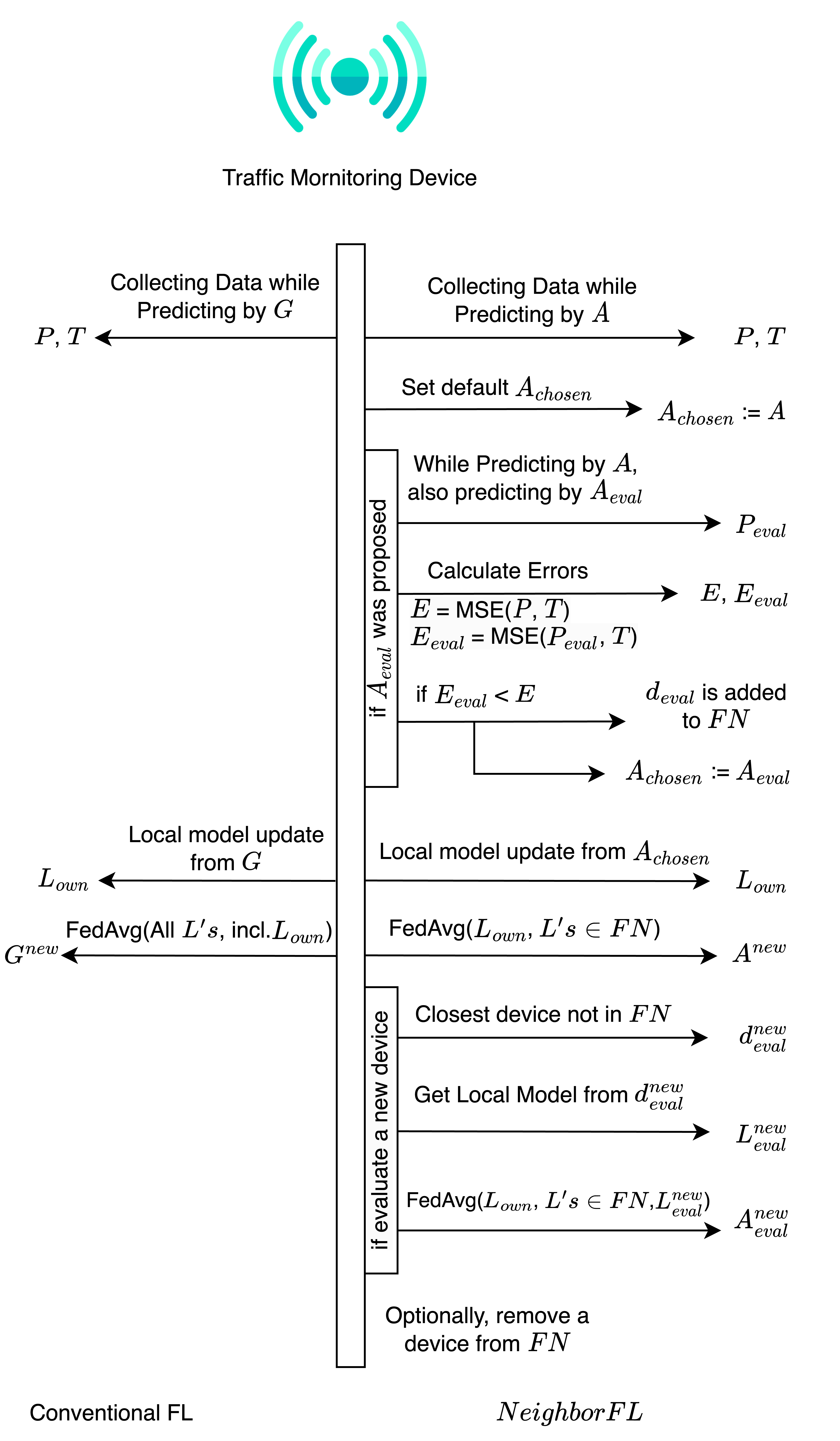
Figure 1 depicts the above steps of NeighborFL throughout a communication round, utilizing mean squared error as the error metric and adopting FedAvg [19] for local model aggregation. Additionally, it offers a parallel comparison with the workflow of the conventional FL approaches.
The objective of NeighborFL is to enable devices to collaboratively search for an improved model that leads to lower prediction errors in the present round. This collaborative effort takes into account the spatial relationship among devices, aiming to enhance the predictions made in the subsequent round considering the temporal conditions. The contributions of NeighborFL and the distinct differences from existing FLTP architectures are summarized as follows:
-
•
Personalized Aggregated Models. Instead of starting the learning process from a single global model generated in the previous communication round, our approach first employs a personalized aggregated model for prediction and another aggregated model for evaluation if a is proposed. Then, each device tests these two models and selects the one with the lower prediction error to continue learning. This approach enables the system to adapt more effectively to real-time traffic dynamics.
-
•
Radius-based Candidate Selection. A device can set a radius to confine its candidate Favorite Neighbors, limiting the maximum number of local models that will be used to produce the aggregated model. This restriction prevents a device from requesting the local models of spatially distant devices, thereby avoiding potential communication delays, exploiting cooperative edge computing infrastructure, and improving the response time of the entire system.
-
•
Knowledge Propagation. The Favorite Neighbors sets of two nearby devices may contain overlapping devices. As a result, a local model from one device can still propagate its learned knowledge to a distant device, even if the distant device does not have the corresponding owner in its Favorite Neighbors set. This propagation of knowledge across devices employs natural weightings to local models during aggregation, facilitating the dissemination of valuable insights and, thereby, enhancing the overall predictive capabilities of the system.
-
•
Individual Device Perspective. NeighborFL allows the devices to explore the spatial and temporal correlation between other participants to form dynamic and individualized groups, rather than considering the entire cohort of devices statically. This device-centric approach builds upon prior research and has the potential to directly incorporate decentralized, device-level model cross-validation to enhance system robustness and resilience [20].
We conducted comprehensive simulations to evaluate the effectiveness of NeighborFL. Without the loss of generality, we chose traffic speed data from 26 detectors in the publicly available PEMS-BAY reference dataset [21], and used the Long Short-Term Memory (LSTM) [22] recurrent neural network as the client model architecture. In addition to using a randomly initialized global model across each of the 26 devices, we also investigated the impact of pretraining the initial model in NeighborFL [23]. For this, we allowed each of the 26 devices to pretrain their initial models using the traffic speed data from the first week of January 2017. We then analyzed the real-time learning and prediction capabilities of NeighborFL by testing its performance over the following two-week period involving both the pretrained and non-pretrained initial models. The experimental results presented in Section IV demonstrate that NeighborFL outperforms the three baseline models in terms of real-time prediction capability in the majority of cases, as indicated by the lower prediction error. Our NeighborFL code repository is available at https://github.com/hanglearning/NeighborFL, and our experiments can be reproduced by the provided portion of the dataset and the specified random seed.
The remainder of this paper is organized as follows. Section II provides a comprehensive review of related work that has guided us in the development of NeighborFL. Section III presents the problem definitions for the key components of NeighborFL and provides a detailed outline of the workflow. Experimental results are presented in Section IV. Section V addresses certain limitations of the current NeighborFL design and proposes potential directions for future research. Section VI summarizes the key findings of the paper.
II Related Work
In this section, we review the existing TP architectures by categorizing them into three general categories - centralized methods, non-streaming FL methods, and streaming FL methods. Both centralized and non-streaming FL methods are further differentiated into methods with and without the grouping mechanism.
II-A Centralized methods
II-A1 Non-grouping
Research in TP has a long history and has become a crucial component of Intelligent Transportation Systems. Early conventional TP models, such as the autoregressive integrated moving average (ARIMA) [24] and exponential smoothing [25], have been used to forecast short-term traffic based on previous observations. In recent years, deep learning-based approaches have gained popularity. Lv et al. (2015) introduced a stacked autoencoder model [3], while Fu et al. (2016) were among the first to utilize LSTM and GRU neural networks [26] for traffic flow prediction. The LSTM and GRU models proposed in [26] demonstrated superior prediction performance compared to the ARIMA model, solidifying the foundation of recurrent neural networks in TP.
II-A2 Grouping
The -nearest neighbor (KNN) is one of the most widely used grouping mechanisms in the TP literature. One of the first uses of KNN in TP research can be found in [11], where its capability for improving TP was analyzed using freeway data. The forecasting method with KNN involves computing the average of predictions from a traffic node’s -nearest neighbors and its own. However, the authors concluded that “the KNN method performed comparably to, but not better than, the linear time-series approach, and further research is needed to delineate those situations where the KNN approach may be preferable.” In 2012, Chang et al. proposed a KNN-based non-parametric regression (KNN-NPR) TP model to address situations where current or future traffic data exhibits fluctuations or abrupt changes. The proposed model demonstrated effectiveness and easy optimization for minimizing prediction errors [12]. Furthermore, Luo et al. (2019) introduced a model named KNN-LSTM, which utilized KNN to select the most relevant neighboring traffic nodes with respect to a specific node. The final prediction results are obtained by weighting the LSTM prediction values from all stations in addition to its own output[13]. We observed that NeighborFL shares a similar methodology with KNN-LSTM in terms of fusing the prediction values. However, in KNN-LSTM, the value specifying the number of neighboring traffic nodes to consider for any given node remains constant. In contrast, our Favorite Neighbors set dynamically expands and shrinks as communication rounds progress.
These works have demonstrated that considering the spatiotemporal correlation characteristics of traffic data can improve the prediction performance of individual nodes. They also inspired us to incorporate distance as a heuristic when a traffic node searches for a Favorite Neighbor.
II-B Non-streaming FL methods
II-B1 Non-grouping
An early application of FLTP was introduced by Liu et al. (2020) [6], where the authors proposed a FL-based architecture for TP using Gated Recurrent Units (GRU) [27], termed FedGRU. FedGRU demonstrated comparable prediction performance to centralized GRU methods while addressing privacy concerns associated with the traffic dataset. Qi et al. (2021) further advanced FLTP by integrating it into a blockchain architecture [7]. This framework addresses the single-point-of-failure issue in centralized FLTP and leverages smart contract technology to safeguard against malicious attacks and ensure high-quality training data. Zhang et al. (2021) extended FLTP by incorporating Graph Neural Networks (GNN) and proposing an adjacency matrix aggregation approach, enabling local GNN-based models to access the global network for improved training effectiveness [2].
II-B2 Grouping
The same work by Liu et al. (2020) introduced an ensemble clustering-based FedGRU algorithm that utilizes traffic data with improved spatio-temporal correlation based on location information. This approach enhances prediction accuracy compared to the standard FedGRU method. It also handles scenarios where multiple clients collaborate to train a traffic prediction model by grouping traffic nodes into clusters prior to applying FedGRU [6]. Zeng et al. (2021) developed a divisive hierarchical clustering approach to partition traffic data at each traffic node into clusters. They applied FL to collaboratively train learning models for each cluster across all stations. The authors demonstrated improved prediction performance compared to the standard FL method using the PeMS dataset [16]. Furthermore, GNN-based methods are also explored as heuristics to group traffic nodes into non-overlapping clusters in [14] and [15].
Although these FLTP frameworks paved the way for exploring privacy-preserving distributed learning in TP, they lack the ability to update the global model in real-time after deployment, making them unable to adapt to changing traffic dynamics, such as non-recurrent traffic incidents and varying traffic patterns. We categorize these FLTP frameworks as non-streaming FL methods since they do not use real-time streaming traffic data for training or updating the models.
II-C Streaming FL methods
In contrast to non-streaming FL approaches, streaming FL architectures rely on real-time traffic data streams to provide inputs for learning and evaluation, allowing for live updates and continuous adaptation. Our research identified two streaming FLTP models. Meese et al. (2022, 2024) introduced BFRT, a streaming Blockchained FL workflow for TP that defines a protocol for federated models to predict real-time traffic volume while collecting live data. By comparing it with a per-device centralized model, the authors demonstrated that the streaming FL method exhibits lower real-time prediction error, highlighting the advantages of collaborative real-time learning [5, 28]. Subsequently, Liu et al. (2023) proposed FedOSTC, an alternative streaming FLTP workflow that incorporates a Graph Attention Network to assess spatial correlation among traffic nodes. It also integrates a period-aware aggregation mechanism to combine local models optimized using the Online Gradient Descent (OGD) algorithm [4]. FedOSTC outperforms five chosen baselines in terms of prediction performance on the partial PEMS-BAY and METR-LA datasets [29].
To the best of our knowledge, there has been no published work focusing on streaming FLTP methods involving grouping, i.e., personalized aggregation, and NeigborFL aims to fill this research gap and lays the foundation for multiple research directions discussed in Section V.
III System Modules
In this section, we present NeighborFL’s key modules and their formulations, along with their implementation in pseudocode.
III-A System Entity
NeighborFL is operated by a set of traffic monitoring devices in the study region through communication rounds . Each device has a unique device ID and sequence number. We assume that a device is equipped with sensor(s) to collect traffic data such as volume, speed, and occupancy, and we also assume a device can act as a computational node to perform model training and participate in other algorithmic operations at the network edge.
III-B Candidate and Favorite Neighbors
The concept of Favorite Neighbors distinguishes NeighborFL from other FLTP frameworks. In NeighborFL, a device aggregates local models from itself plus its Favorite Neighbors (Algo. 10: line 21) instead of using the local models from all the participants (i.e., ). Prior to joining NeighborFL, a device initializes an empty set called FN to keep track of its favorite neighbors (Algo. 10: line 5) and a radius value to populate a hashmap called CFN to record its candidate favorite neighbors (Algo. 1: lines 9-11).
A single candidate favorite neighbor is denoted as . A device considers neighboring devices within a distance of as candidates. The key in CFN represents the device ID of the , while the associated value is the Haversine distance between the and the device (Algo. 1: lines 8, 11). In this work, a device’s becomes its favorite neighbor () after evaluating the real-time prediction error, as described in Sec. III-C4. The evaluation order is determined by the Haversine distance between the device and , from closest to farthest (Algo. 1: line 15; Algo. 2: line 4), with a retry interval control mechanism (Algo. 1: lines 4-6, 12-14; Algo. 2: lines 5-8; Algo. 6: lines 15-17) explained in Sec. III-C4. Algo. 1 outlines the process of populating CFN for the -th device , while Algo. 2 explains how a may be selected by in for evaluation based on the relative Haversine distance. Note that different devices may choose different values for , and specifically represents the value chosen by device in Algo. 1. represents the selected to be evaluated by in (Algo. 2: line 7).
Technically, a device has the option to set as unlimited to consider all devices in the study region. However, selecting an appropriate value for can enhance a device’s operational efficiency, and the overall system scalability, by restricting the number of candidate neighbors. This is important because distant devices located on different roads may display distinctly different traffic patterns, decreasing the evaluation efficiency. Also note that a device might consider evaluating more than one candidate. Without loss of generality, we concentrate on the scenario where only one is evaluated at a time in this study (Algo. 2, lines 6-8).
III-C Online Streaming Model
NeighborFL is designed to operate in real-time regarding data collection, training, and prediction. This section provides formal definitions for these three aspects.
III-C1 Online Streaming Data Collection
Each device collects traffic data in real-time for training, prediction, and evaluation when participating in NeighborFL. We denote as a single traffic data point, and as the -th traffic data point collected by device in communication round . This data point, , represents a scalar value such as traffic volume or speed (Algo. 3: line 6). We define as the total number of data points that a device needs to collect within the (Algo. 3: line 5). Each device is equipped with a memory card to store the collected data, and the collection of the data points stored in the memory of is represented as . To mitigate overfitting with outdated data, the length of is limited to a maximum size called MaxDataSize. This ensures that data from older rounds is excluded from training in the current round (Algo. 3: lines 9-11). The algorithm for real-time data collection and updating is presented in Algo. 3. represents the updated during or after the completion of .
III-C2 Online Training
As mentioned in Sec. I, at the end of a communication round, a device utilizes the selected aggregated model and the updated for training and generating its updated local model (Algo. 4, lines 7-11). We define a training instance as , where represents a vector containing a continuous sequence of traffic data points from . The variable can be either a scalar value or a vector, depending on the desired number of output forecasting horizon (i.e., prediction steps) , and the length of depends on the number of input units of the model. At any moment, the number of training instances in can be calculated as
| (1) |
For example, in this work, we employed an LSTM neural network with 12 input units () and 1 output unit (), representing a 1-step look-ahead prediction. Let be the -th data point in and be the -th training instance. Suppose a device has collected at least MaxDataSize data points and consider MaxDataSize = 72, then the first training instance in can be expressed as , and the last training instance, corresponds to the -th instance as calculated in Eq. 1, can be written as . The process of updating the local model of in using the defined local epoch numbers and a batch size of 1 is outlined in Algo. 4.
III-C3 Real-time Prediction
In round , device makes one real-time prediction for the next time steps (denoted as ) using an aggregated model from , denoted as , on the most recent data points from (denoted as ) (Algo. 5: lines 10-12), prior to collecting a new data point (Algo. 5: lines 13-14). Consequently, the number of predictions made by a device within the second communication round () and onwards is equal to the number of newly collected data points, which is denoted by (Algo. 3: line 5; Algo. 5: lines 6-14). As a special case, in the first communication round (), a device needs to collect at least data points to make the first prediction (Algo. 5: line 7-8), and data points to initiate local learning111To ensure that there is a sufficient amount of data for training, it can be inferred that the value of MaxDataSize also needs to be larger than or equal to . (Algo. 4, line 6, Algo. 5: line 15). Therefore, must be at least to ensure a local model is produced at the end of . Note that denotes the number of data points (i.e., ’s) stored in , and the maximum value of is MaxDataSize. Consequently, the number of predictions a device makes in would equal to
| (2) |
which is similar to the calculation of the number of data instances in as expressed in Eq. 1.
The steps for real-time prediction by in are described in Algo. 5. The resulting ground truth consists of instances of actual traffic data points (denoted as ) corresponding to the prediction instances (i.e., ) in . Specifically, each ground truth instance (Algo. 5: line 16) or prediction instance (Algo. 5: line 11) is represented by a scalar value or a vector, depending on the value of , and is recorded in chronological order in or , respectively, controlled by over time within a communication round (Algo. 5: lines 6-7, 15, 18). and will be utilized to demonstrate the evaluation of a candidate favorite neighbor in Sec. III-C4.
III-C4 Evaluation of a candidate neighbor
As mentioned in Sec. III-B, a device’s candidate favorite neighbor () becomes its favorite neighbor () based on real-time prediction error evaluation (Algo. 6: lines 11-12). Inspired by the concept of reinforcement learning and the general approach to training a neural network by minimizing inference errors, the following process occurs:
If a device is selected for evaluation by device in round (Algo. 2: line 7), in round will evaluate an aggregated model that integrates the local model of , denoted as (Algo. 10: lines 18-19, 24-25). This evaluation involves the comparison of the prediction error , derived by applying an error metric between and (Algo. 6, line 7), and another prediction error , obtained by assessing against (Algo. 6, line 8). is comprised of the predictions made by (Algo. 10: lines 15-16), which includes while being produced (Algo. 10: lines 24-25), whereas are composed of the predictions made by (Algo. 10: line 14), which does not include (Algo. 10: line 21). In simpler terms, a device determines the effectiveness of a potential candidate neighbor device by incorporating its local model into an aggregated model for making predictions. It then compares the error from these predictions to the error from another aggregated model that excludes the neighbor’s local model. The prediction error metric (Algo. 6, lines 7-10) used for evaluation could be any commonly used measure in traffic prediction models, such as MAE, MRE, MSE, RMSE, among others [3, 6]. An example of device-level MSE calculation for is given in Eq. 3.
If is found to be lower than , indicating that contributes positively to the prediction in , adds to its favorite neighbor set (Algo. 6: lines 11-12), and will be chosen to perform local update at the end of (Algo. 6: line 13), meanwhile will be included to produce (Algo. 10: line 25). Otherwise, records and updates its evaluation round in a hashmap named .last_try_round (Algo. 6: line 15), and will be chosen to perform local update (Algo. 6: line 17). Additionally, increments the retry interval of in another hashmap .retry_interval (Algo. 6: line 16), in which all of ’s candidate favorite neighbors are assigned an initial retry interval value of 0 (Algo. 1: line 13). The same pattern of retry interval incrementation occurs when is tried again in subsequent rounds without being favored. The combination of last_try_round and retry_interval forms the retry control mechanism for NeighborFL. This mechanism prevents a (i.e., a specific ) from being frequently retried without considering other available candidate neighbors (Algo. 2, lines 5-8). Taking inspiration from reinforcement learning, this mechanism can be seen as a form of penalty that delays the future inclusion of a local model from an evaluated candidate that fails to contribute effectively to the timely prediction process. Note that the retry pattern (Algo. 6, lines 15-16) can be designed differently, such as decreasing the retry interval if is re-added to and remains there for an extended period.
The evaluation process of by in round , is defined in Algo. 6. The output represents the chosen aggregated model to perform local update at the end of (Algo. 6, lines 13, 17). Algo. 6 also involves calculating the reputation for (Algo. 6, lines 9-10), which will be used to illustrate a favorite neighbor removal method in Sec. III-D2.
In situations where , handling the instances in , and requires special consideration to align the error calculations correctly (Algo. 6, lines 7-8). Table. I illustrates the global sequence number of data points collected in and the global sequence number of the predicted values in by a random device following Algorithm 5 for , during , and , with and . For example, when and during the 4th step (i.e., , Algo. 5, line 6) in , according to Algo. 5, a device would first predict the 28th and 29th traffic values (Algo. 5, lines 10-12), denoted as the prediction instance in green. Then, it collects the 28th true data point (Algo. 5, lines 13-14), colored in gray, and extracts the 27th and 28th true data points from (Algo. 5, line 16) denoted as the truth value instance in yellow. Note that in are omitted from the table as the devices haven’t started training nor real-time prediction during those steps.
From the table, it can be inferred that for , the sequences of the data points in the instances of and differ by one position. Specifically, the first prediction instance in corresponds to the 2nd truth instance in . Similarly, for , the first in corresponds to the 3rd in . In general, fthe corresponding in of the in is shifted by positions in terms of index.
To ensure that accommodates data collection shifts correctly while evaluating a candidate’s local model in , , one approach could be to let infer the latest predictions in using the historical data and append these ’s to the beginning of , and also append the latest ’s of to . This way, the indexes of the sequences in , , and will align. A simpler alternative is to drop the first ’s in and drop the last ’s in both and , as shown in pink in Table. I for examples with and . Using this method, we can maintain the evaluation of after finishes collecting new data during . Note that by using this approach, has to be at least .
| Collect | ||||||||
|---|---|---|---|---|---|---|---|---|
| 13 | 13th | 13 | 13 | NULL | 13, 14 | NULL | 13, 14, 15 | |
| 14 | 14th | 14 | 14 | 13, 14 | 14, 15 | NULL | 14, 15, 16 | |
| 15 | 15th | 15 | 15 | 14, 15 | 15, 16 | 13, 14, 15 | 15, 16, 17 | |
| 16 | 16th | 16 | 16 | 15, 16 | 16, 17 | 14, 15, 16 | 16, 17, 18 | |
| 17 | 17th | 17 | 17 | 16, 17 | 17, 18 | 15, 16, 17 | 17, 18, 19 | |
| 18 | 18th | 18 | 18 | 17, 18 | 18, 19 | 16, 17, 18 | 18, 19, 20 | |
| 19 | 19th | 19 | 19 | 18, 19 | 19, 20 | 17, 18, 19 | 19, 20, 21 | |
| 20 | 20th | 20 | 20 | 19, 20 | 20, 21 | 18, 19, 20 | 20, 21, 22 | |
| 21 | 21st | 21 | 21 | 20, 21 | 21, 22 | 19, 20, 21 | 21, 22, 23 | |
| 22 | 22nd | 22 | 22 | 21, 22 | 22, 23 | 20, 21, 22 | 22, 23, 24 | |
| 23 | 23rd | 23 | 23 | 22, 23 | 23, 24 | 21, 22, 23 | 23, 24, 25 | |
| Round 1 | 24 | 24th | 24 | 24 | 23, 24 | 24, 25 | 22, 23, 24 | 24, 25, 26 |
| 1 | 25th | 25 | 25 | 24, 25 | 25, 26 | 23, 24, 25 | 25, 26, 27 | |
| 2 | 26th | 26 | 26 | 25, 26 | 26, 27 | 24, 25, 26 | 26, 27, 28 | |
| 3 | 27th | 27 | 27 | 26, 27 | 27, 28 | 25, 26, 27 | 27, 28, 29 | |
| 4 | 28th | 28 | 28 | 27, 28 | 28, 29 | 26, 27, 28 | 28, 29, 30 | |
| 5 | 29th | 29 | 29 | 28, 29 | 29, 30 | 27, 28, 29 | 29, 30, 31 | |
| 6 | 30th | 30 | 30 | 29, 30 | 30, 31 | 28, 29, 30 | 30, 31, 32 | |
| 7 | 31th | 31 | 31 | 30, 31 | 31, 32 | 29, 30, 31 | 31, 32, 33 | |
| 8 | 32th | 32 | 32 | 31, 32 | 32, 33 | 30, 31, 32 | 32, 33, 34 | |
| 9 | 33th | 33 | 33 | 32, 33 | 33, 34 | 31, 32, 33 | 33, 34, 35 | |
| 10 | 34th | 34 | 34 | 33, 34 | 34, 35 | 32, 33, 34 | 34, 35, 36 | |
| 11 | 35th | 35 | 35 | 34, 35 | 35, 36 | 33, 34, 35 | 35, 36, 37 | |
| Round 2 | 12 | 36th | 36 | 36 | 35, 36 | 36, 37 | 34, 35, 36 | 36, 37, 38 |
| 1 | 37th | 37 | 37 | 36, 37 | 37, 38 | 35, 36, 37 | 37, 38, 39 | |
| 2 | 38th | 38 | 38 | 37, 38 | 38, 39 | 36, 37, 38 | 38, 39, 40 | |
| 3 | 39th | 39 | 39 | 38, 39 | 39, 40 | 37, 38, 39 | 39, 40, 41 | |
| 4 | 40th | 40 | 40 | 39, 40 | 40, 41 | 38, 39, 40 | 40, 41, 42 | |
| 5 | 41st | 41 | 41 | 40, 41 | 41, 42 | 39, 40, 41 | 41, 42, 43 | |
| 6 | 42nd | 42 | 42 | 41, 42 | 42, 43 | 40, 41, 42 | 42, 43, 44 | |
| 7 | 43rd | 43 | 43 | 42, 43 | 43, 44 | 41, 42, 43 | 43, 44, 45 | |
| 8 | 44th | 44 | 44 | 43, 44 | 44, 45 | 42, 43, 44 | 44, 45, 46 | |
| 9 | 45th | 45 | 45 | 44, 45 | 45, 46 | 43, 44, 45 | 45, 46, 47 | |
| 10 | 46th | 46 | 46 | 45, 46 | 46, 47 | 44, 45, 46 | 46, 47, 48 | |
| 11 | 47th | 47 | 47 | 46, 47 | 47, 48 | 45, 46, 47 | 47, 48, 49 | |
| Round 3 | 12 | 48th | 48 | 48 | 47, 48 | 48, 49 | 46, 47, 48 | 48, 49, 50 |
III-D Removal of a favorite neighbor
With evolving traffic conditions, including non-recurrent events, seasonal variations, or route detours, neighboring devices can undergo substantial changes in traffic dynamics. Consequently, the local models derived from these devices may no longer contribute effectively or may even adversely impact the real-time predictions made by a given device that opts to include them in its favorite neighbors set (FN). Thus, the removal of poor performing favorite neighbors from a device’s FN becomes crucial in maintaining accurate real-time predictions. In this section, we introduce our design of the removal mechanism, which includes two parts: a removal trigger and a removal method. However, it should be noted that this design is presented as an example and alternative approaches can be explored when implementing NeighborFL in practice.
III-D1 Removal Trigger
The removal trigger is responsible for determining when a device should initiate the removal action for one or more favorite neighbors () from its favorite neighbors set (FN). In the current design, the trigger is activated when the prediction error of a device increases over a specified number of continuous rounds, denoted as (Algo. 9, line 3).
III-D2 Removal Method
We propose two distinct removal methods in this work: “remove by reputation” and “remove the last added”. In the “remove by reputation” method, each device maintains a hashmap called rep_book (Algo. 1, lines 6, 14; Algo. 6, line 10; Algo. 7) to track the subjective reputation of its candidate favorite neighbors (’s). The reputation is determined by calculating the difference between and when a is evaluated as (Algo. 6, line 9). If the difference is a positive value, indicating that the local model of () contributes to reducing the real-time prediction error, is assigned a positive reputation. Conversely, if is negative, receives a negative reputation (Algo. 6, line 10). The reputation accumulates over the course of communication rounds when a is being (re-)evaluated. When a device removes a , it eliminates the associated with the lowest reputation (Algo. 7, lines 6-8). Algo. 7 illustrates the process of “remove by reputation” executed by . A removed is denoted as ~.
The “remove the last added” method allows a device to remove in the reverse order of their addition, effectively undoing the addition of a . As a device typically (but not definitely) adds to FN from closest to farthest, the device usually removes from farthest to closest (Algo. 8: lines 4-5), following a similar heuristic as Algo. 2. In this method, a device keeps track of the order in which ’s are added to its FN, and always removes the most recently added . In this method, the FN data structure utilizes a stack instead of a set. This method intuitively exhibits a more chronological adaptation to time-dependent changes compared to the “remove by reputation” method. Algo. 8 outlines the process of the “remove the last added” method performed by , assuming the removal of one at a time.
Lastly, to avoid rapid re-evaluation and addition of a ~ in subsequent communication rounds, a device must maintain a record of ~ in its last_try_round and retry_interval hashmap (Algo. 9, lines 5-6). The complete favorite neighbor removal steps are described in Algo. 9.
III-E NeighborFL complete operations
The preceding subsections have divided NeighborFL into various modules. This section consolidates those operations and presents the overall top-to-bottom functioning of NeighborFL in Algo. 10. Along with forming the CFN hash map, a device also initializes five variables (Algo. 10, lines 5-9). The initial model provided to the devices in is denoted by , which can be randomly generated or pretrained. Different devices may have different initial models, and thus denotes the initial model of before it participates in NeighborFL (Algo. 10, line 8).
The first three actions a device performs upon starting a new communication round are to make two predictions while collecting the incoming data points to update its local dataset (Algo. 10: lines 13-16). It is important to underscore that these three functions operate concurrently in an asynchronous manner, governed by the shared time stamp variable (Algo. 3, lines 3, 5, 8; Algo. 5, lines 3, 6, 18), as well as . The Aggregate() function takes a device’s freshly produced local model and the local models from its Favorite Neighbors to perform model aggregation and generate (Algo. 10, line 21), typically using a method like Federated Averaging [19]. If an available candidate is selected, the same aggregation method should also be used to produce (Algo. 10, lines 24-25). Also note that the removal action should occur before a device selects an available candidate (Algo. 10, lines 22-23). This is done to prevent a scenario where a newly selected candidate has the lowest reputation and gets removed immediately after being chosen, particularly when a device adopts the “remove by reputation” method.
IV Experimental Results
IV-A Experimental Design
IV-A1 Dataset
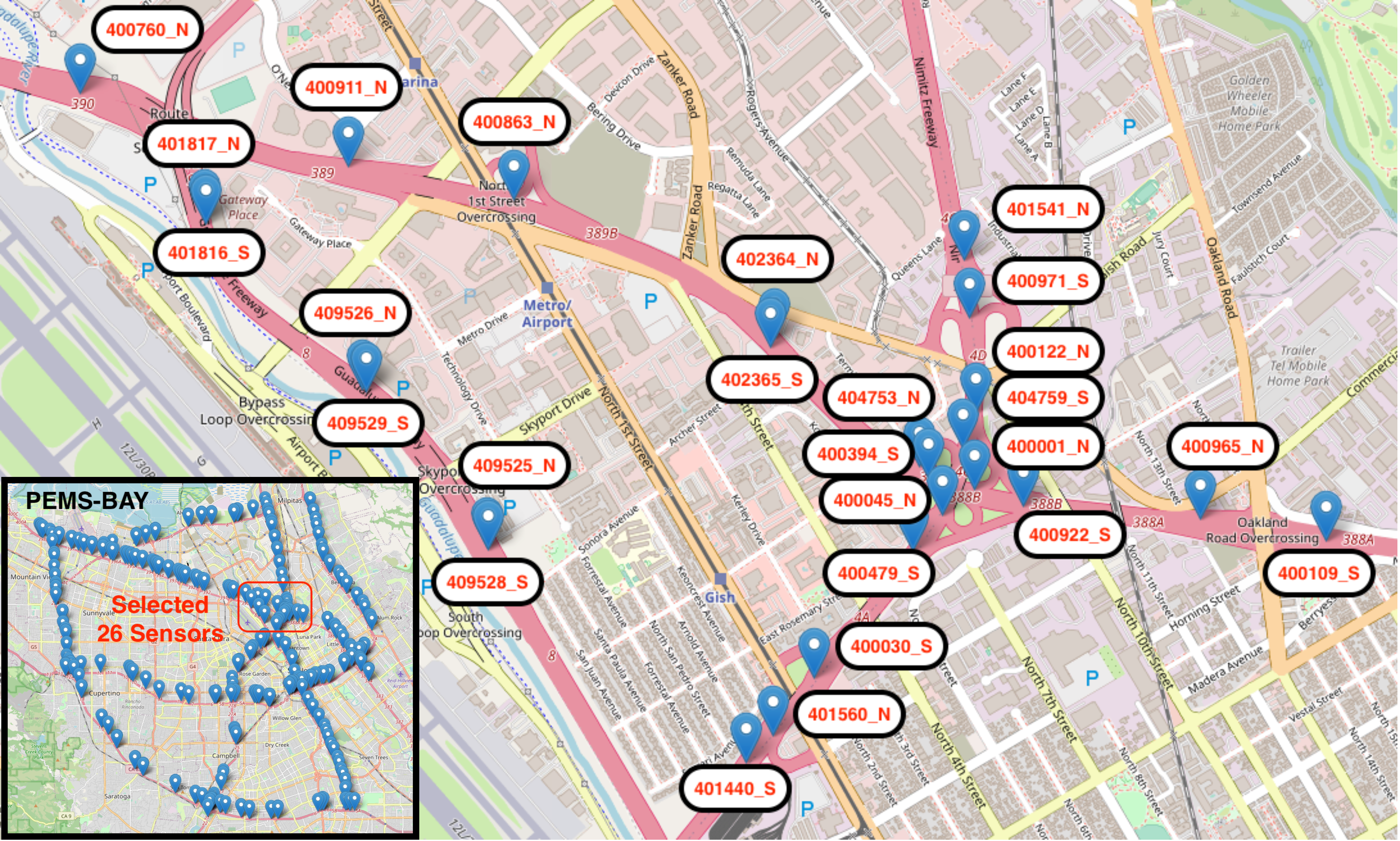
We manually selected a study region from the widely available reference dataset, PEMS-BAY[21], collected by the California Transportation Agency Performance Measurement System (PeMS). Our chosen area covers 26 devices from the total 325 devices within the dataset. In Fig. 2, the locations of all 325 devices are shown in the lower left corner. The devices included in our experiments are enclosed within the red region, and their corresponding device IDs are labeled next to the devices’ locations in the remainder of the figure, showing a zoomed-in map. Each device’s ID includes an underscore followed by the letter “N” or “S” to indicate the traffic direction it monitors, either North or South. Without loss of generality, we use traffic speed as the modeling variable in this study.
IV-A2 Deep Learning Model
In our experiments, we employed a light-weight construction of the Long Short-Term Memory (LSTM) [22] variety of recurrent neural network (RNN) because it can be efficiently trained on heterogeneous edge devices for FLTP applications [26, 30, 6, 5, 7, 28]. Following the convention of federated learning, all devices utilized identical LSTM networks. These networks consisted of 12 input neurons (), corresponding to one hour of traffic data with a 5-minute time resolution, and one output neuron (), enabling a one-step 5-minute look-ahead prediction, as discussed in Sec. III-C2. The LSTM network is constructed with two hidden layers of size 128 hidden units. Furthermore, the two LSTM layers are followed by a dropout layer initialized at and a fully connected output layer of size .
IV-A3 Baseline Methods
To assess the performance of NeighborFL, we conducted a comparative analysis with three baseline methods: Centralized, NaiveFL, and r-NaiveFL. These baseline methods are also streaming methods and exhibit the following distinctions compared to NeighborFL:
-
a)
The Centralized model of a device undergoes continuous real-time training without federation at the end of each communication round. From this perspective, the Central model trained by a device can be seen as updated solely by this specific device’s incoming data throughout the entire process. This model was initially introduced in [5], and its performance highlighted here serves to emphasize the benefits of adopting federated learning for traffic prediction. Technically, we can interpret the training process of a Central model as a device performing NeighborFL where the Faviorite Neighbors set remains empty indefinitely.
-
b)
The NaiveFL model is also updated online in real-time and follows the conventional FL aggregation method. In every communication round, all devices share the same aggregated (global) model for prediction and learning. It serves as the primary model for comparison with NeighborFL, emphasizing the effectiveness of the aggregation heuristics employed in NeighborFL. Note that the conventional FL approach, represented on the left side of Fig. 1, illustrates the workflow of NaiveFL. Formally, we can think of the training process of a NaiveFL model in this context as a device implementing NeighborFL where its Favorite Neighbors set includes the entire cohort of devices in the study region, excluding itself, from the onset of the FL process.
-
c)
The r-NaiveFL model can be viewed as a hybrid between NeighborFL and NaiveFL. Essentially, the training process of a r-NaiveFL model, when performed by a device, involves filling its Favorite Neighbors set with devices within its radius (used to form its Candidate Favorite Neighbors set), excluding itself, at initialization. Notably, unlike NaiveFL, r-NaiveFL still enables each device to have a customized aggregated model for training and prediction in each communication round. As both r-NaiveFL and NeighborFL select devices from the same area for federation, with the only difference being that NeighborFL dynamically adjusts a device’s Favorite Neighbors set, we present the performance of r-NaiveFL to further highlight the effectiveness of the heuristics employed in NeighborFL and the benefits of evolutionary Favorite Neighbors sets.
IV-A4 Number of Predictions
In most traffic datasets, including PEMS-BAY [32] used in this study, the time resolution is set to 5 minutes. To align the communication round with hours, we set to 12 for and subsequent rounds. This indicates that a device needs to collect 12 data points and makes 12 one-step look-ahead predictions in , corresponding to one hour of data in the PEMS-BAY dataset. However, because the LSTM models employed in this study have 12 input neurons and a single output neuron, they require a minimum of data points to form the online training batch and begin learning. Consequently, we set to 24 to ensure is satisfied in , which is equivalent to 2 hours of data. This configuration allows devices to make 24 - 12 - 1 + 1 = 12 predictions in (Algo. 5: lines 5-8, 10-12), as calculated by Eq. 2, thereby unifying the number of predictions for all communication rounds to be 12.
IV-A5 NeighborFL Setup
For the NeighborFL method, we conducted experiments using four different favorite neighbor removal strategies to assess their impact on prediction performance. These strategies were compared while keeping other parameters consistent. The four strategies are summarized as follows:
-
1.
Remove-by-reputation (Algo. 7) with a removal trigger of (referred to as R1).
-
2.
Remove-by-reputation (Algo. 7) with a removal trigger of (referred to as R3).
-
3.
Remove-the-last-added (Algo. 8) with a removal trigger of (referred to as L1).
-
4.
Remove-the-last-added (Algo. 8) with a removal trigger of (referred to as L3).
Furthermore, we used a fixed radius ( = 1 mile) for all devices to form their Candidate Favorite Neighbors Set (CFN). The number of candidate favorite neighbors (#CFN) for each device is listed in Table II.
| Device ID | #CFN | Device ID | #CFN |
|---|---|---|---|
| 401816_S | 8 | 401817_N | 8 |
| 400911_N | 10 | 400863_N | 18 |
| 409526_N | 13 | 409529_S | 13 |
| 409525_N | 21 | 409528_S | 21 |
| 402364_N | 21 | 402365_S | 21 |
| 401541_N | 16 | 400971_S | 19 |
| 400122_N | 19 | 404759_S | 19 |
| 400394_S | 19 | 404753_N | 19 |
| 400045_N | 19 | 400001_N | 18 |
| 400922_S | 18 | 400479_S | 19 |
| 400030_S | 20 | 401560_N | 19 |
| 401440_S | 18 | 400965_N | 16 |
| 400109_S | 12 | 400760_N | 6 |
For example, device 400760_N has 6 candidate favorite neighbors (401817_N, 400911_N, 401816_S, 400863_N, 409526_N, 409529_S) within a 1-mile radius, which is consistent with Fig. 2.
Additionally, we set MaxDataSize = 72 for all devices, which corresponds to 6 hours of traffic data. The Mean Squared Error (MSE) was used to evaluate the real-time prediction error of a candidate neighbor’s local model (Algo. 6, lines 9-10), as we want a device to skip a candidate neighbor’s model producing large errors. Moreover, as pretrained models have previously been utilized to initialize the models used in FLTP applications [33, 14], we have also evaluated the effects of pretraining on the performance of NeighborFL and the three baseline methods. In the experiments involving pretrained models, we used the first week of traffic speed data from PEMS-BAY (ranging from 2017-01-01 00:00:00 to 2017-01-07 23:55:00, both timestamps included) as training data for each of the 26 sensors. We trained 26 models individually using an LSTM network with randomly initialized weights (represented as ) with the structure mentioned in IV-A2, applying 5 local epochs and a batch number of 1. The resulting trained models are denoted as , , …, and serve as the initial models for each corresponding device in real-time federated learning. For experiments involving non-pretrained models, each device uses as its initial model.
Our simulations were performed on Google Colab using an NVIDIA Tesla T4 GPU with standard RAM. The files containing the experimental results mentioned in Sec. IV-A6 are available in our GitHub repository and can be reproduced using a random seed value of 40.
IV-A6 Results
We conducted a total of 250 communication rounds across 26 devices for all of our experiments, which involved both pretrained and non-pretrained initial models. Within each of these two running types, we employed three baseline methods and four different configurations of NeighborFL (R1, R3, L1, L3), resulting in a total of 14 running methods, as indicated in Table. III and Table. V. These 250 rounds utilized speed data for training from 2017-01-08 00:00:00 to 2017-01-18 10:55:00 (both timestamps inclusive), and the devices provided real-time predictions for speed values from 2017-01-08 01:00:00 to 2017-01-18 10:55:00 (both timestamps inclusive).
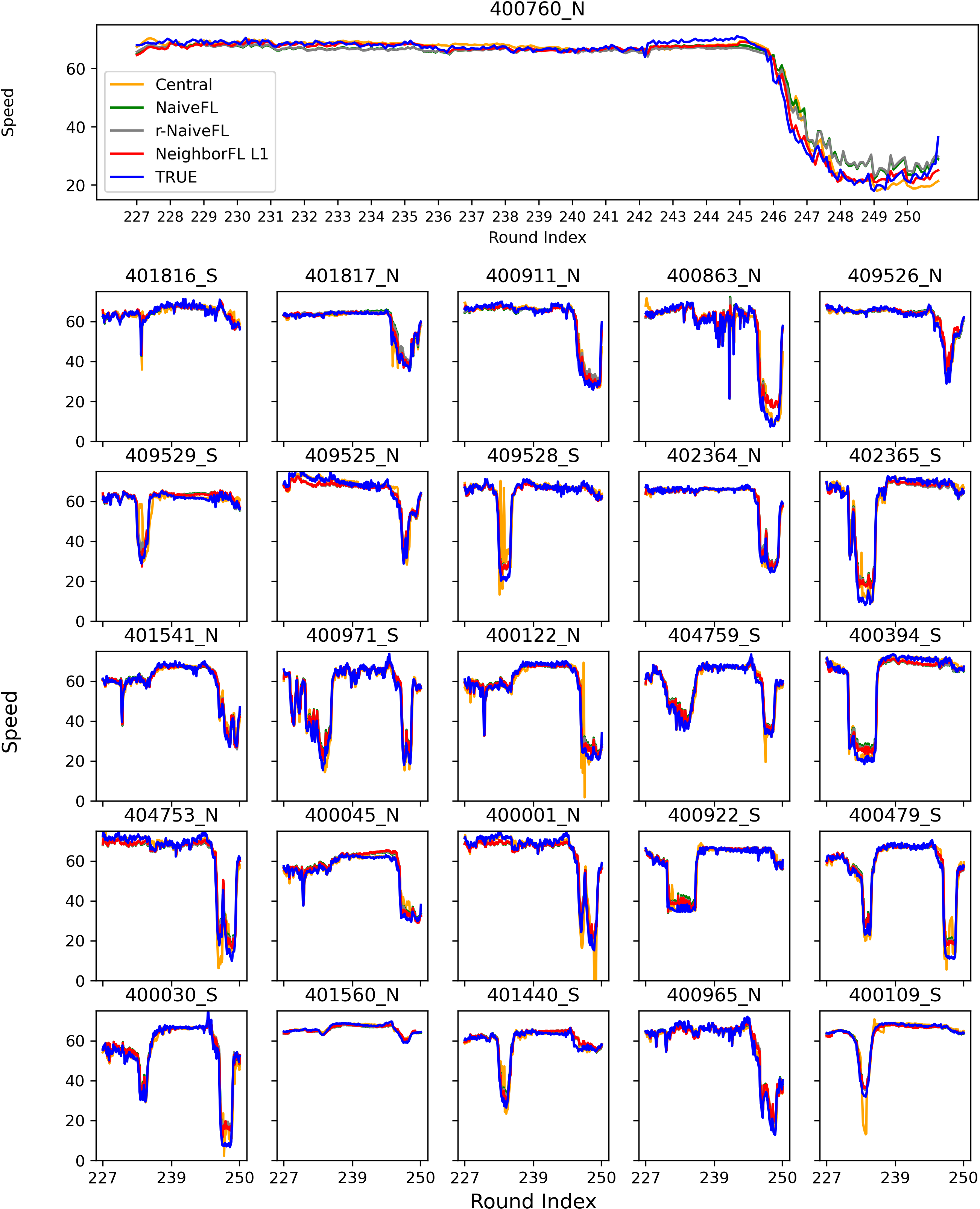
To visually compare the real-time prediction accuracy among these methods, we have plotted the real-time prediction curves (i.e., values in , Algo. 10, line 13) alongside the ground truth curves (i.e., values in , Algo. 10, line 13) for the last 24 hours of the simulated federation (i.e., rounds 227 to 250). Due to space constraints, we presented the curves from three baseline and the NeighborFL L1 methods under the pretrained setting, as shown in Fig. 3. The criteria for choosing these four out of the 14 methods are referred to Table. III, which outlines the average device mean squared error (MSE) across all 26 devices for the last 24 rounds between the ground truth values and the corresponding methods.
As an example of the calculation of the average device MSE values for any of these 14 methods shown in Table. III, the Pretrain MSE value of NeighborFL L1 (i.e., 7.45 highlighted in pink in Table. III) is computed as follows:
-
1.
First, we calculate the MSE value between the NeighborFL L1 predictions and the corresponding ground truth values from rounds 227 to 250 for each of the 26 devices. For a random device , the MSE value is obtained by following Eq. 3,
(3) Where:
In this case, , , ; corresponds to of NeighborFL L1, and represents the truth values extracted from the raw PEMS-BAY dataset [21] of with the associated device ID for the corresponding time range. The resulting MSE values for each of the 26 devices are listed under the NeighborFL L1 column in Table. IV.
-
2.
These individual device MSE values are then summed up and divided by the number of devices in to obtain the average device MSE value, as shown in Eq. 4.
(4) In this case, , and the resulting value for NeighborFL L1 is 7.45, serving as an overall last 24 hours error evaluation metric. The same calculation procedure is applied to generate the other 13 average MSE values presented in Table III.
From Table. III, we observe that NeighborFL L1 had the smallest Average Device MSE value (highlighted in pink) among all 14 methods. In the pretrained setting, all four NeighborFL configurations exhibited lower average MSE values compared to the three baseline methods, highlighting the superior real-time learning and prediction capabilities of NeighborFL. For instance, NeighborFL L1 reduces the MSE value by 16.9% compared to NaiveFL. A similar trend is observed in the non-pretrained setting, where NeighborFL L3 achieves the lowest average MSE value (highlighted in green) among all methods. Although the MSE value of r-NaiveFL (i.e., 10.88) is lower than that of NeighborFL L1 and NeighborFL R3, the difference is marginal, and all four NeighborFL configurations outperformed NaiveFL by at least 5%, while also significantly outperforming Central under the non-pretrained setting. Furthermore, by comparing the Average Device MSE values of the seven methods between the pretrained and non-pretrained settings, we observed that using pretrained models can significantly enhance the training and prediction performance for all seven configurations. Specifically, for NeighborFL, pretraining the initial models with one week of historical data can reduce the prediction error by at least 30%, as indicated in the table.
| Methods | Pretrain MSE | Non-Pretrain MSE |
|---|---|---|
| Central | 13.14 | 19.53 |
| NaiveFL | 8.97 | 11.01 |
| r-NaiveFL | 8.35 | 10.88 |
| NeighborFL L1 | 7.45 | 10.9 |
| NeighborFL L3 | 7.83 | 10.38 |
| NeighborFL R1 | 7.8 | 10.5 |
| NeighborFL R3 | 7.74 | 10.89 |
In Fig. 3, the curves representing the speed predictions produced by Central, NaiveFL, and r-NaiveFL methods are shown in orange, green, and gray, respectively. The curve of the NeighborFL L1 method is depicted in red, while the ground truth curve is displayed in blue. The x-axis represents the communication round, with each round consisting of 12 steps of speed measurements between any two round indexes, since we chose and . By closely examining the curves of the representative device 400760_N, we can observe that the NeighborFL method consistently achieves better overall predictions compared to the three baseline methods. The red curve is generally closer to the blue curve compared to the other three curves, which is particularly evident during rounds 246 to 250. Moreover, NeighborFL demonstrates enhanced adaptability to sudden speed changes detected by the device, as evidenced by the 12 speed steps in the round 246 to 247 segment. This trend is also observed in other devices such as 401817_N, 400911_N, 409529_S, and 400922_S.
To further assess the performance of NeighborFL at an individual device level, we provide the MSE values for each of the 26 devices over the last 24 rounds, categorized by the different methods, in Table IV. In each device’s row, the lowest MSE value is highlighted in green. By counting the number of green highlights under the NeighborFL L1 column, we observe that out of the 26 devices, NeighborFL outperforms all three baseline methods in 18 devices. For the remaining 8 devices, 5 devices (i.e., 400394_S, 400045_N, 400001_N, 401560_N, 400109_S) still have their NeighborFL outperform NaiveFL method. Overall, NeighborFL surpasses NaiveFL in 88% of the devices within the entire cohort during the last 24 hours of the simulations.
| Central | NaiveFL | r-NaiveFL | NeighborFL L1 | |
| 401816_S | 6.81 | 2.69 | 2.98 | 3.14 |
| 401817_N | 4.59 | 5.36 | 4.88 | 2.65 |
| 400911_N | 10.56 | 6.81 | 7.47 | 5.31 |
| 400863_N | 41.67 | 33.61 | 32.9 | 31.31 |
| 409526_N | 4.29 | 3.76 | 3.47 | 6.55 |
| 409529_S | 24.14 | 4.51 | 5.01 | 3.57 |
| 409525_N | 8.03 | 7.43 | 7.41 | 7.08 |
| 409528_S | 42.1 | 5.4 | 5.1 | 5.09 |
| 402364_N | 5.18 | 6.03 | 5.79 | 5 |
| 402365_S | 15.43 | 17.24 | 15.75 | 13.46 |
| 401541_N | 6.4 | 4.58 | 4.35 | 4.3 |
| 400971_S | 14.74 | 14.77 | 13.21 | 13.01 |
| 400122_N | 22.8 | 7.78 | 6.69 | 5.73 |
| 404759_S | 8.27 | 7.19 | 6.37 | 5.99 |
| 400394_S | 5.52 | 13.14 | 10.68 | 8.6 |
| 404753_N | 18.9 | 14.65 | 13.24 | 11.16 |
| 400045_N | 5.99 | 5.66 | 5.35 | 5.47 |
| 400001_N | 21.36 | 10.14 | 9.41 | 9.6 |
| 400922_S | 7.08 | 6.56 | 5.42 | 4.96 |
| 400479_S | 16.59 | 12.09 | 10.21 | 9.84 |
| 400030_S | 13.93 | 15.67 | 15.09 | 11.69 |
| 401560_N | 0.47 | 0.76 | 0.74 | 0.66 |
| 401440_S | 9.37 | 4.39 | 4.03 | 3.67 |
| 400965_N | 8.08 | 10.25 | 9.98 | 10.63 |
| 400109_S | 12.19 | 2.02 | 1.27 | 1.94 |
| 400760_N | 7.09 | 10.75 | 10.23 | 3.22 |
Another way to visualize the performance of NeighborFL compared to the three baselines is to examine the overall trend of MSE throughout the entire simulation (i.e., from communication round 1 to 250). In Fig. 4, we present how the MSE values of the predictions generated by the three baselines and NeighborFL L1 change in relation to the ground truth for each of the 26 devices as the communication round progresses. The color scheme for the four methods follows that of Fig. 3. Unlike Fig. 3, the y-axis represents the MSE value, and the x-axis represents round ranges instead of individual round indexes. Each round range represents a group of round indexes, such as Round Range 24-48 indicating communication rounds 24, 25, 26, …, 48 (inclusive). We group the error values into round ranges to fit the curves within the small subfigures while preserving the true trends. Each round range consists of 24 communication rounds, except for the first round range which has 23 rounds (due to the absence of predictions in the initial hour of the simulation), and the last round range which has 10 rounds. The calculation of these MSE values follows the same formula as Eq. 3.
Each plot also includes three percentage values displayed at the top. These percentages indicate the number of times NeighborFL L1 achieves a lower MSE value than the corresponding baseline method across the 11 smoothed MSE values within the respective round ranges on the x-axis, for a particular device. For example, for device 409529_S, NeighborFL L1 produces MSE values that are lower than Central 6 times and lower than both NaiveFL and r-NaiveFL 8 times, resulting in percentages of 6/11=54.55% and 8/11=72.73%, respectively. When a percentage value exceeds 50%, the corresponding method and the percentage are highlighted in red, indicating that NeighborFL L1 outperforms the particular baseline method for the majority of the simulation. Notably, for devices where NeighborFL L1 outperforms NaiveFL by more than 50%, a star is displayed in the upper left corner of the figure.
The device 400922_S has been selected as the representative for this analysis. By examining the error curves of 400922_S, we can clearly observe that the error of NeighborFL L1 consistently remains lower than the three baseline methods, as indicated by the highlighted red values. Among the remaining 25 devices, we have seen that 22 devices outperform NaiveFL according to the stars, further highlighting the effectiveness of NeighborFL compared to NaiveFL.
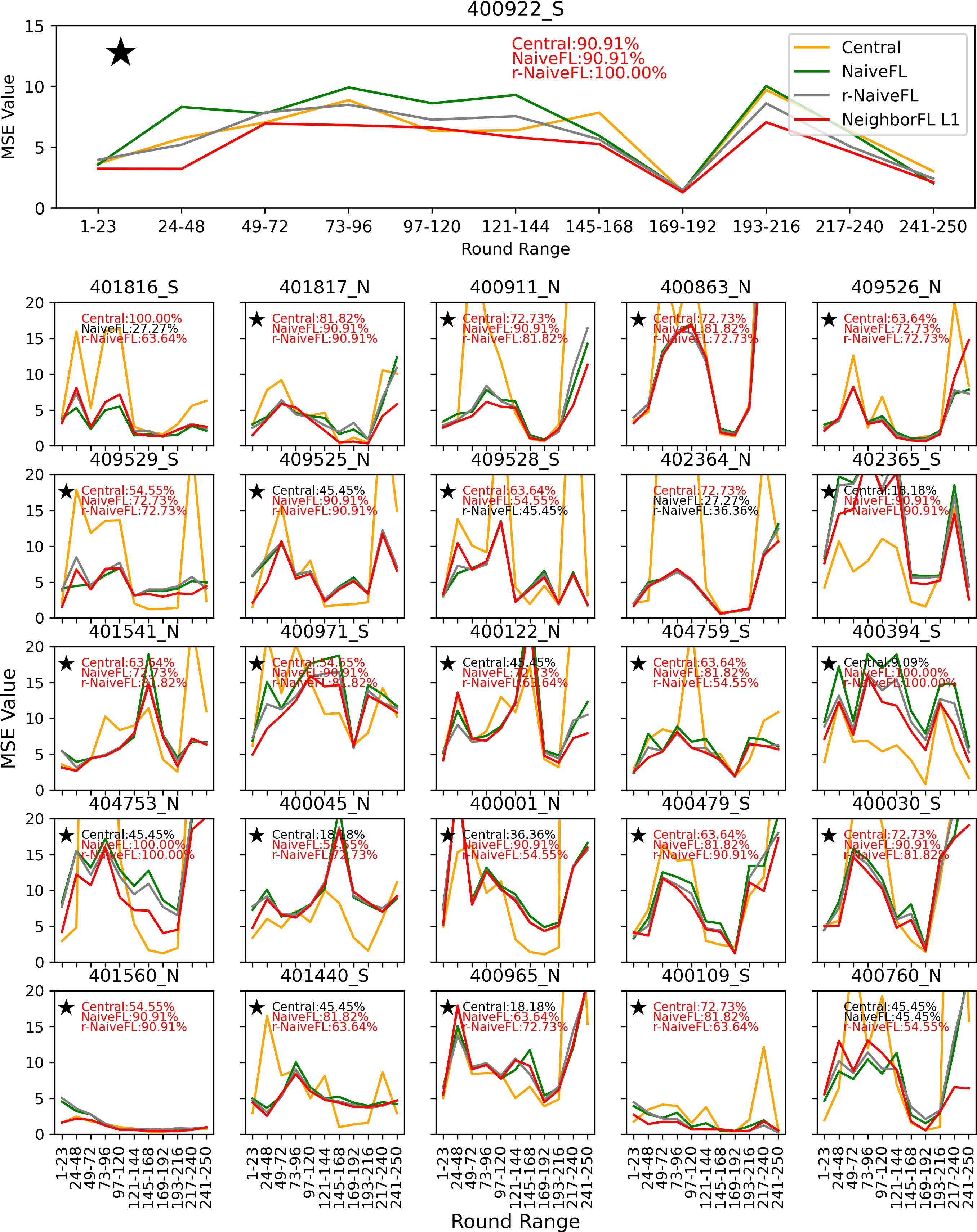
While it is noticeable that the error of the Central method exhibits greater fluctuations in certain devices such as 401816_S, 400911_N, 409529_S, 402364_N, 400109_S, we also observed that 10 out of 26 devices have their Central method outperforming NeighborFL L1 over 50% of the times. This is particularly evident for devices such as 402365_S, 400394_S, 400045_N, and 400965_N. In fact, the Central method produces the best results for these four devices compared to NaiveFL, r-NaiveFL, and NeighborFL. Our preliminary hypothesis is that 402365_S, 400394_S, and 400045_N are all located on the same small segment of highway. Their location in the network, as shown in Fig. 2, is a critical junction connecting two major highways, likely experiencing severe bottleneck congestion during rush periods. The prediction plots for 402365_S and 400394_S in Fig. 3 show a severe drop in speed around the round 235 period, which is inconsistent with most other sensors. In the future, it would be desirable for the enhanced NeighborFL to autonomously recognize such scenarios and avoid performing any type of federation to at least match the performance of the Central method. Potential solutions for addressing this issue will be discussed in Section V.
Table. V presents the Average Device MSE values for the 26 devices across the 250 rounds, categorized by the prediction methods. The calculation of those average MSE values follows the same procedure as the values shown in Table. III. It is worth noting that the Central method generally exhibits much larger average MSE values compared to the FL methods. Additionally, we observe that, under both pretrained and non-pretrained settings, the average MSE values for all four configurations of NeighborFL (highlighted in green) outperform the baseline methods. Since the average MSE values among the four NeighborFL configurations are very close, and different removal methods may be developed to adapt to specific traffic situations, we have omitted the comparison analysis among the four removal methods of NeighborFL.
| Methods | Pretrain MSE | Non-Pretrain MSE |
|---|---|---|
| Central | 10.82 | 22.19 |
| NaiveFL | 7.73 | 18.36 |
| r-NaiveFL | 7.44 | 17.7 |
| NeighborFL L1 | 6.77 | 14.99 |
| NeighborFL L3 | 7.11 | 15.8 |
| NeighborFL R1 | 6.57 | 15.43 |
| NeighborFL R3 | 6.98 | 16.11 |
V Discussion and Future Work
In this section, we explore potential solutions for NeighborFL to outperform the Central method in certain situations and enhance the overall performance of NeighborFL as a whole. Additionally, we present two potential future research directions to extend NeighborFL.
V-A Improving the performance of NeighborFL
As shown in Fig. 4, there are 10 devices where the Central method outperforms all three types of federated methods most of the time, including our best run of NeighborFL. However, it is important to note that NeighborFL L1 still outperforms NaiveFL in 9 out of these 10 devices. Despite the fact that the Central method exhibits the largest Average Device MSE throughout the entire execution, as shown in Table. III, we aim to address this issue and elevate the performance of NeighborFL to be on par with Central for our future work. One primary drawback of NeighborFL is the lack of direct consideration of local traffic trends within the candidate radius when evaluating or removing candidates, instead relying on one-time error evaluation and time- or reputation-based removal. Ignoring the sensor’s purpose and the properties of the observed road segment may degrade the model performance for some clients. One potential solution is to reset a device’s favorite neighbor set (FN) entirely if its real-time prediction error continuously increases, allowing NeighborFL to operate similarly to the Central method for an extended period and recalibrate by re-evaluating its candidate favorite neighbors from scratch. Another advanced approach is to incorporate local traffic trend analysis and road segment properties into the evaluation criteria for candidate selection. In conclusion, experimenting with novel neighbor evaluation heuristics and/or favorite neighbor removal mechanisms will be key design choices to enhance the performance of NeighborFL.
V-B Predicting the impacts of Non-Recurrent Events
Intelligent Transportation Systems often involve predicting the impacts of non-recurrent events such as bad weather conditions or sports events on traffic congestion and delays [34]. Fig. 3 demonstrates that NeighborFL exhibits better adaptability to sudden traffic dynamic changes compared to the selected baseline methods. Moreover, with its support for multi-horizon prediction capabilities, we believe that NeighborFL has the potential to predict the impacts of non-recurrent events. By training NeighborFL on traffic datasets that include non-recurrent events, the system may rapidly adjust a device’s FN to include only those devices within its radius that would be affected by these changes. This adaptation can lead to more accurate short-term traffic predictions precisely when non-recurrent events occur. Thus, NeighborFL shows promise in predicting the effects of such events and improving real-time traffic management.
V-C Detecting malfunctioning detectors
As NeighborFL enables devices to remove certain favorite neighbors when real-time prediction errors increase, it opens up the potential for detecting malfunctioning detectors. In practice, a group of devices within a specific area could share information about their removed favorite neighbors. If a particular device consistently appears in most removal reports, there is a high probability that it is a malfunctioning detector. In such cases, the devices can report this finding to the traffic management center, prompting a repair order. Moreover, nearby devices can also be proactive by temporarily excluding the malfunctioning detector from their favorite neighbors set for an extended period. By incorporating such mechanisms, NeighborFL contributes to improved traffic management and enhanced overall system reliability.
VI Conclusion
The paper presents NeighborFL, a decentralized Federated Learning-based approach for real-time traffic prediction, leveraging spatial-temporal relationships among detectors. The methodology enables devices to dynamically allocate personalized groups for model aggregation based on real-time prediction errors, mitigating the non-IID issues of traffic data collected in different locations and enhancing prediction performance by up to 16.9% compared to the naive FL setting. Future research will explore additional neighbor evaluation heuristics and favorite neighbor removal mechanisms to further enhance prediction accuracy, predict impacts of non-recurrent events, and detect malfunctioning detectors. NeighborFL shows potential for efficient and adaptable Intelligent Transportation Systems, benefiting commuters and traffic management agencies.
References
- [1] X. Yuan, J. Chen, J. Yang, N. Zhang, T. Yang, T. Han, and A. Taherkordi, “Fedstn: Graph representation driven federated learning for edge computing enabled urban traffic flow prediction,” IEEE Transactions on Intelligent Transportation Systems, 2022.
- [2] C. Zhang, S. Zhang, J. James, and S. Yu, “Fastgnn: A topological information protected federated learning approach for traffic speed forecasting,” IEEE Transactions on Industrial Informatics, vol. 17, no. 12, pp. 8464–8474, 2021.
- [3] Y. Lv, Y. Duan, W. Kang, Z. Li, and F.-Y. Wang, “Traffic flow prediction with big data: A deep learning approach,” IEEE Transactions on Intelligent Transportation Systems, vol. 16, no. 2, pp. 865–873, 2014.
- [4] Q. Liu, S. Sun, M. Liu, Y. Wang, and B. Gao, “Online spatio-temporal correlation-based federated learning for traffic flow forecasting,” arXiv preprint arXiv:2302.08658, 2023.
- [5] C. Meese, H. Chen, S. A. Asif, W. Li, C.-C. Shen, and M. Nejad, “Bfrt: Blockchained federated learning for real-time traffic flow prediction,” in 2022 22nd IEEE International Symposium on Cluster, Cloud and Internet Computing (CCGrid). IEEE, 2022, pp. 317–326.
- [6] Y. Liu, J. James, J. Kang, D. Niyato, and S. Zhang, “Privacy-preserving traffic flow prediction: A federated learning approach,” IEEE Internet of Things Journal, vol. 7, no. 8, pp. 7751–7763, 2020.
- [7] Y. Qi, M. S. Hossain, J. Nie, and X. Li, “Privacy-preserving blockchain-based federated learning for traffic flow prediction,” Future Generation Computer Systems, vol. 117, pp. 328–337, 2021.
- [8] Q. Sun, W. Liu, D. Huynh, and M. Reynolds, “Graph embeddings for non-iid data feature representation learning,” in Data Mining: 20th Australasian Conference, AusDM 2022, Western Sydney, Australia, December 12–15, 2022, Proceedings. Springer, 2022, pp. 43–57.
- [9] L. Li, D.-c. Zhan, and X.-c. Li, “Aligning model outputs for class imbalanced non-iid federated learning,” Machine Learning, pp. 1–24, 2022.
- [10] X. Ma, J. Zhu, Z. Lin, S. Chen, and Y. Qin, “A state-of-the-art survey on solving non-iid data in federated learning,” Future Generation Computer Systems, vol. 135, pp. 244–258, 2022.
- [11] G. A. Davis and N. L. Nihan, “Nonparametric regression and short-term freeway traffic forecasting,” Journal of Transportation Engineering, vol. 117, no. 2, pp. 178–188, 1991.
- [12] H. Chang, Y. Lee, B. Yoon, and S. Baek, “Dynamic near-term traffic flow prediction: system-oriented approach based on past experiences,” IET intelligent transport systems, vol. 6, no. 3, pp. 292–305, 2012.
- [13] X. Luo, D. Li, Y. Yang, and S. Zhang, “Spatiotemporal traffic flow prediction with knn and lstm,” Journal of Advanced Transportation, vol. 2019, 2019.
- [14] C. Zhang, S. Zhang, S. Yu, and J. James, “Graph-based traffic forecasting via communication-efficient federated learning,” in 2022 IEEE Wireless Communications and Networking Conference (WCNC). IEEE, 2022, pp. 2041–2046.
- [15] T. Qi, L. Chen, G. Li, Y. Li, and C. Wang, “Fedagcn: A traffic flow prediction framework based on federated learning and asynchronous graph convolutional network,” Applied Soft Computing, vol. 138, p. 110175, 2023.
- [16] T. Zeng, J. Guo, K. J. Kim, K. Parsons, P. Orlik, S. Di Cairano, and W. Saad, “Multi-task federated learning for traffic prediction and its application to route planning,” in Proc. of the IEEE Intelligent Vehicles Symposium (IV), 2021, pp. 451–457.
- [17] T. Yang, G. Andrew, H. Eichner, H. Sun, W. Li, N. Kong, D. Ramage, and F. Beaufays, “Applied federated learning: Improving google keyboard query suggestions,” arXiv preprint arXiv:1812.02903, 2018.
- [18] L. Lyu, Y. Shen, and S. Zhang, “The advance of reinforcement learning and deep reinforcement learning,” in 2022 IEEE International Conference on Electrical Engineering, Big Data and Algorithms (EEBDA). IEEE, 2022, pp. 644–648.
- [19] B. McMahan, E. Moore, D. Ramage, S. Hampson, and B. A. y Arcas, “Communication-efficient learning of deep networks from decentralized data,” in Artificial intelligence and statistics. PMLR, 2017, pp. 1273–1282.
- [20] H. Chen, S. A. Asif, J. Park, C.-C. Shen, and M. Bennis, “Robust blockchained federated learning with model validation and proof-of-stake inspired consensus,” AAAI 2021 Workshop - Towards Robust, Secure and Efficient Machine Learning, 2021.
- [21] Y. Li, R. Yu, C. Shahabi, and Y. Liu, “Diffusion convolutional recurrent neural network: Data-driven traffic forecasting,” in International Conference on Learning Representations (ICLR ’18), 2018.
- [22] S. Hochreiter and J. Schmidhuber, “Long short-term memory,” Neural computation, vol. 9, no. 8, pp. 1735–1780, 1997.
- [23] Y. Tan, G. Long, J. Ma, L. Liu, T. Zhou, and J. Jiang, “Federated learning from pre-trained models: A contrastive learning approach,” Advances in Neural Information Processing Systems, vol. 35, pp. 19 332–19 344, 2022.
- [24] M. S. Ahmed and A. R. Cook, Analysis of freeway traffic time-series data by using Box-Jenkins techniques, 1979, no. 722.
- [25] B. M. Williams, P. K. Durvasula, and D. E. Brown, “Urban freeway traffic flow prediction: application of seasonal autoregressive integrated moving average and exponential smoothing models,” Transportation Research Record, vol. 1644, no. 1, pp. 132–141, 1998.
- [26] R. Fu, Z. Zhang, and L. Li, “Using lstm and gru neural network methods for traffic flow prediction,” in 2016 31st Youth Academic Annual Conference of Chinese Association of Automation (YAC). IEEE, 2016, pp. 324–328.
- [27] K. Cho, B. Van Merriënboer, C. Gulcehre, D. Bahdanau, F. Bougares, H. Schwenk, and Y. Bengio, “Learning phrase representations using rnn encoder-decoder for statistical machine translation,” arXiv preprint arXiv:1406.1078, 2014.
- [28] C. Meese, H. Chen, W. Li, D. Lee, H. Guo, C.-C. Shen, and M. Nejad, “Adaptive traffic prediction at the its edge with online models and blockchain-based federated learning,” IEEE Transactions on Intelligent Transportation Systems, 2024.
- [29] Y. Wu, D. Zhuang, A. Labbe, and L. Sun, “Inductive graph neural networks for spatiotemporal kriging,” in Proceedings of the AAAI Conference on Artificial Intelligence, vol. 35, no. 5, 2021, pp. 4478–4485.
- [30] C. Meese, D. Lee, H. Chen, and M. Nejad, “vloft: Variable learning rate for online federated traffic prediction,” in 2023 IEEE 26th International Conference on Intelligent Transportation Systems (ITSC), 2023, pp. 4247–4253.
- [31] G. Hinton, N. Srivastava, and K. Swersky, “Neural networks for machine learning lecture 6a overview of mini-batch gradient descent,” Cited on, vol. 14, no. 8, p. 2, 2012.
- [32] C. Chen, Freeway performance measurement system (PeMS). University of California, Berkeley, 2002.
- [33] C. Zhang, L. Cui, S. Yu, and J. James, “A communication-efficient federated learning scheme for iot-based traffic forecasting,” IEEE Internet of Things Journal, vol. 9, no. 14, pp. 11 918–11 931, 2021.
- [34] F. Aljuaydi, B. Wiwatanapataphee, and Y. H. Wu, “Deep learning-based prediction models for freeway traffic flow under non-recurrent events,” in 2022 8th International Conference on Control, Decision and Information Technologies (CoDIT), vol. 1. IEEE, 2022, pp. 815–820.
| Symbol | Definition |
|---|---|
| The -th traffic device in the Device Set | |
| The -th communication round | |
| A candidate favorite neighbor belonging to the Candidate Favorite Neighbors set of . CFN is an ordered hash map of {Key: a ’s Device ID, Value: the Haversine distance between the and }, sorted by value from low to high (close to far Haversine distance). | |
| A favorite neighbor belonging to the Favorite Neighbors set (or stack data structure) of | |
| The radius value taken by to form its CFN | |
| A selected by in for evaluation in | |
| The dataset of traffic data points collected by until the end of , bounded by MaxDataSize | |
| MaxDataSize | The maximum size of data points stored in |
| The number of data points a device collects within a communication round, and also the number of predictions a device makes in and onwards | |
| A traffic data point. denotes the -th data point collected by in | |
| The number of input units in the model used for federated learning, where | |
| The number of output units in the model used for federated learning, where | |
| A data instance in . is a vector of data points with size , and can be a scalar value or a vector of data points depending on the value of | |
| The latest data points from a device uses to perform a prediction for the next steps | |
| One prediction instance with a size of using as the input to the model | |
| A local model. In , denotes the local model of , and denotes ’s local model | |
| Shared global model produced at the end of a communication round in conventional FL | |
| An aggregated model. denotes the model produced by taking and local models from devices in , and denotes the model produced by aforementioned models plus . denotes the initial model of before participating in NeighborFL | |
| The number of local training epochs | |
| Prediction instances, i.e., a list of ’s. denotes the predictions produced by , and denotes the predictions produced by or | |
| One ground truth data instance with a size of from the real-time updated | |
| Ground truth instances, i.e., a list of ’s. represents the data values collected by in | |
| Prediction error, which could be MAE, MRE, MSE, RMSE, etc. denotes the prediction error calculated by and , and is the error calculated by and | |
| ~ | A removed favorite neighbor from a device’s FN set |
| The number of continuous rounds of a device’s real-time prediction error increase required to trigger a favorite neighbor removal action | |
| .rep_book | A hash map for to keep track of the reputation of its ’s. The reputation of a is calculated as when it is being evaluated as a |
| .last_try_round | A hash map for to keep track of the (re-)evaluation round for when is being removed or skipped from being added to due to failure in reducing the prediction error |
| .retry_interval | A hash map for to keep track of and examine the retry interval for a when is being considered for selection as a |
Biographies
![[Uncaptioned image]](/html/2407.12226/assets/figures/hang_headshot.jpg) |
Hang Chen received his B.S. degree in Computer Science from the University of Delaware, USA, in 2015, where he is currently pursuing his Ph.D. degree. His research interests span distributed ledger technology, federated learning consensus design, deep networks cross-validation, and intelligent transportation systems. |
![[Uncaptioned image]](/html/2407.12226/assets/figures/cmeese_headshot3.jpg) |
Collin Meese (Student Member, IEEE) received his B.S. degree in computer science from the University of Delaware in 2020. He is currently a Ph.D. student at the University of Delaware. His research interests include blockchain, distributed machine learning, intelligent transportation systems, connected and autonomous vehicles. He is an NSF GRFP Fellow and a student member of IEEE. |
![[Uncaptioned image]](/html/2407.12226/assets/figures/mnejad.jpg) |
Mark Nejad (Senior Member, IEEE) is an Associate Professor at the University of Delaware. His research interests include network optimization, distributed systems, blockchain, game theory, and intelligent transportation systems. He has published more than fifty peer-reviewed papers and received several publication awards, including the 2016 IISE Pritsker Best Doctoral Dissertation award and the 2019 CAVS Best Paper award from the IEEE VTS. His research is funded by the National Science Foundation and the Department of Transportation. He is a member of the IEEE and INFORMS. |
![[Uncaptioned image]](/html/2407.12226/assets/x1.png) |
Chien-Chung Shen (Member, IEEE) received the B.S. and M.S. degrees from National Chiao Tung University, Taiwan, and the Ph.D. degree from the UCLA, all in computer science. He was a Research Scientist at Bellcore Applied Research, working on the control and management of broadband networks. He is currently a Professor with the Department of Computer and Information Sciences, University of Delaware. His research interests include blockchain, Wi-Fi, SDN and NFV, ad hoc and sensor networks, dynamic spectrum management, cybersecurity, distributed computing, and simulation. He was a recipient of the NSF CAREER Award and a member of the ACM. |