Probabilistic Reachability of Stochastic Control Systems:
A Contraction-Based Approach
Abstract
In this paper, we propose a framework for studying the probabilistic reachability of stochastic control systems. Given a stochastic system, we introduce a separation strategy for reachability analysis that decouples the effect of deterministic input/disturbance and stochastic uncertainty. A remarkable feature of this separation strategy is its ability to leverage any deterministic reachability framework to capture the effect of deterministic input/disturbance. Furthermore, this separation strategy encodes the impact of stochastic uncertainty on reachability analysis by measuring the distance between the trajectories of the stochastic system and its associated deterministic system. Using contraction theory, we provide probabilistic bounds on this trajectory distance and estimate the propagation of stochastic uncertainties through the system. By combining this probabilistic bound on trajectory distance with two computationally efficient deterministic reachability methods, we provide estimates for probabilistic reachable sets of the stochastic system. We demonstrate the efficacy of our framework through numerical experiments on a feedback-stabilized inverted pendulum.
Keywords: Reachability analysis, Stochastic systems
1 Introduction
Reachability analysis is a fundamental problem in control theory and dynamical systems that studies how the trajectories of a system propagate with time. Reachability analysis has been successfully used in many real-world applications to explore the transient behaviors of systems and to verify their safety over a given time horizon. However, providing formal guarantees for behaviors of dynamical systems using reachability analysis is challenging for several reasons. First, reachability analysis deals with the behavior of an infinite number of trajectories. Consequently, most simulation-based methods are insufficient and theoretical methods are needed to provide guarantees on behavior of the system. Second, practical systems typically operate in uncertain environments, where their behaviors are affected by different types of random and adversarial uncertainties. Therefore, it is crucial to suitably incorporate the effect of various uncertainties in reachability of these systems. Moreover, many real-world systems are large-scale with highly nonlinear dynamics, necessitating computationally efficient and scalable reachability tools to certify their behaviors.
The majority of the research on reachability analysis focuses on control systems with deterministic input/disturbance [1]. By considering the least favorable or the most detrimental values of these input/disturbances, these work perform worst-case uncertainty analysis and provide guarantees for reachable sets of the system under all possible uncertainty scenarios. The classical frameworks for reachability of the systems with deterministic input/disturbance include Hamilton-Jacobi and dynamic programming approaches [2, 3] and the set-propagation approaches such as ellipsoidal methods [4] and polytope method [5, 6]. Despite their deep theoretical foundations, these approaches are either only applicable to certain classes of systems or are not computationally tractable for large-scale systems. Motivated by applications to general large-scale systems with complex components, various computationally efficient and scalable deterministic reachability frameworks have been recently developed in the literature [7]. Examples of these methods include reachability using Lipschitz bound [8], matrix measure-based reachability [9, 10], and interval-based reachability [11, 12, 13, 14].
In many real-world applications, systems are subject to unpredictable and rapidly fluctuating disturbances. For such disturbances, it is impossible to provide precise bounds on their magnitudes. Consequently, worst-case uncertainty analysis either offers no guarantees or results in overly conservative estimates of the reachable sets. Instead, it is more reasonable to model these disturbances as stochastic variables and use probabilistic methods for reachability analysis of the system. However, the reachability analysis of stochastic systems is significantly more challenging than that of deterministic systems due to the probabilistic nature of their evolution. Several frameworks have been developed in the literature to analyze the propagation of uncertainties in stochastic systems. Hamilton-Jacobi and dynamic programming approaches characterize probabilistic reachability as a the solution of a game between two players [15, 16, 17]. Despite their generality, a significant drawback of these reachability approaches lies in their computational heaviness, rendering them impractical for reachability analysis of large-size systems. Recent works have focused on improving the computational complexity of the dynamic programming for reachability of stochastic systems [18]. Functional approaches develop barrier function [19, 20, 21] for measuring the probability of a trajectory staying inside a reachable set. These functional approaches are computationally efficient. However, in applications, they require an exhaustive search for a suitable function and lack the flexibility to balance the accuracy and efficiency of reachability analysis.
In this paper, we develop a computationally efficient framework for probabilistic reachability of control systems with both deterministic input/disturbance and stochastic uncertainty. First, we present a separation strategy that decomposes the effect of deterministic input/disturbance and the effect of stochastic uncertainty on reachability analysis of the stochastic control system. We show that the effect of deterministic input/disturbance on reachability can be captured using reachable sets of an associated deterministic system. This is a key feature of this separation strategy as it allows to use any frameworks for deterministic reachability to study the propagation of deterministic input/disturbance in stochastic systems. The effect of stochastic uncertainty on reachability is represented by the distance between trajectories of the stochastic system and the associated deterministic system. Inspired by the works on incremental stability of stochastic systems [22, 23, 24], we leverage contraction theory to study the evolution of stochastic uncertainty in the system. While the existing literature on contraction analysis of stochastic systems focus on providing conditions for their stability, we establish probabilistic transient bounds on the distance between trajectories of the stochastic system and its associated deterministic system. By combining our probabilistic bound on propagation of stochastic uncertainties with contraction-based and interval-based reachability methods for deterministic systems, we provide high probability bounds on reachable sets of stochastic systems. Finally, we apply our framework with both contraction-based and interval-based deterministic reachability to obtain probabilistic bounds on reachable sets of a feedback stabilized inverted pendulum.
2 Mathematical Preliminaries
Vectors, matrices, and functions
we denote the component-wise vector order on n by , i.e., for , we have if and only if , for every . Given , we define the interval . Given a norm on n, we define the ball with radius centered at by . Given a norm on n and a matrix , the matrix measure of with respect to is defined by , where is the matrix norm on n×n induced from . Given a nonsingular matrix , the -weighted -norm is defined by and the -weighted -matrix measure is denoted by . Given two sets , we define the Minkowski sum of the sets and by . Given , we define the interval . Given a set and a transformation , we define . Given a square matrix , we denote the trace of matrix by . For two matrices , we denote if is a positive definite matrix. Given a continuously differentiable function , we denote the Jacobian of at point by .
Dynamical systems
consider the deterministic system
| (1) |
where is the state of the system, is the input. Depending on the application, the input can be considered as a controller or a disturbance. We assume that is a parameterized vector field which is measurable in and locally Lipschitz in and . Using Rademacher’s theorem, the Jacobian exists for almost every . Given the initial set and the disturbance set , the -reachable set is the set of all possible states the system (1) can achieve at time , i.e.,
| (2) |
It is well known that finding the exact reachable set of general nonlinear systems is computationally intractable [25]. Instead, most existing approaches for reachability focus on efficient methods for over-approximating the reachable sets [1], i.e. finding the set satisfying . Given a norm on n, the deterministic system (1) is contracting with rate with respect to the norm if, for every and every ,
where and are two trajectories of the system (1) with the same input . It can be shown [26, Theorem 36] that the system (1) is contracting with rate with respect to the norm if and only if, for almost every
The function is an inclusion function for the vector field of the system (1) if, for every and every ,
| (3) |
One can show every vector field has at least one inclusion function [13, 27]. However, inclusion function of is not generally unique [27].
3 Problem formulation
In this paper, we study reachability of stochastic control systems with both deterministic input/disturbance and stochastic uncertainty. We consider the stochastic version of the deterministic system (1) given by
| (4) |
where is the state, is the input, is the stochastic uncertainty, and and is a matrix-valued function. We assume that the input belongs to the set , for every , and the stochastic uncertainty is an -dimensional Wiener process (standard Brownian motion). Throughout this paper, we assume that and are measurable in time and locally Lipschitz in to ensure the existence and uniqueness of solutions of the stochastic system (4) and its associated deterministic system (1) [28, Theorem 5.2.1].
Our goal is to provide probabilistic bounds on trajectories of the stochastic control system (4) starting from some with any input . We first present a separation strategy that decouples the effect of deterministic input/disturbance and stochastic uncertainty on reachability of the stochastic system (4). We show that the effect of deterministic input/disturbance on reachability can be captured using the reachable set of the associated deterministic system (1). We represent the effect of stochastic uncertainty on reachability using the distance between trajectories of (4) and their associated trajectories of (1) and leverage contraction theory to establish high probability bounds on this distance.
4 Decomposition of Reachability Analysis
In this section, we study reachability of the control system (4) with both deterministic input/disturbance and stochastic uncertainty. Inspired by the sampling-based approaches for reachability [17, 29, 30], we focus on probabilistic reachable sets of stochastic system (4), i.e., the sets that contain trajectories of the system with certain probability. We develop a separation strategy that presents a novel perspective toward constructing probabilistic reachable sets of stochastic system (4). The key idea in separation strategy is to decouple the effect of deterministic input/disturbance and the effect of stochastic uncertainty on the probabilistic reachable set of (4).
The effect of stochastic uncertainty is encoded in the distance between trajectories of (4) and their associated trajectories of the deterministic system (1). More specifically, for time and probability level , we assume there exists a constant such that, with probability ,
| (5) |
where is a trajectory of the stochastic system (4) with the input starting from an initial condition and is the associated trajectory of the deterministic system (1) with the same input starting from the same initial condition .
The effect of deterministic input/disturbance is captured using the reachable set of the associated deterministic system (1). The probabilistic reachable set of the stochastic system (4) can then be constructed by combining these two components as described in the next theorem.
Theorem 1 (Separation strategy).
Proof.
Remark 1 (Decomposition of probabilistic reachable sets).
Theorem 1 decomposes the probabilistic reachability analysis of the stochastic system (4) into two separate problems: (i) over-approximating reachable sets of the associated deterministic system (1) and, (ii) bounding the propagation of stochastic uncertainty in the system. This decomposition brings considerable flexibility to probabilistic reachablity analysis of (4) as any approach for over-approximating reachable sets of the deterministic system (1) can be used to analyze the effect of deterministic input/disturbance. In general, computing the Minkowski sum of two arbitrary sets can be computationally complicated. However, when the sets are ellipsoids or polytopes, there exist efficient algorithms for estimating their Minkowski sum [31, 32].
Theorem 1 captures the propagation of stochastic uncertainty in reachability using the distance between trajectories of the stochastic system (4) and their associated trajectories of the deterministic system (1) via inequality (5). In the next section, we use incremental stability properties of the stochastic system (4) to bound the constant in (5).
5 Bounds on propagation of stochastic uncertainty
In this section, we provide high confidence bounds on the distance between trajectories of the stochastic system (4) and that of the deterministic system (1). Our approach is based on using contraction properties of the system. We start with the following assumption.
Assumption 1.
There exist a positive definite matrix and constants such that, for almost every ,
-
(i)
, and
-
(ii)
.
Various approaches have been proposed in the literature to efficiently compute upper bounds on including sum-of-square methods [33] and convex-hull methods [10]. These methods can readily extend to compute an upper bound for and to search for the positive definite which gives rise to the optimal constants and . Now, we can state the main result of this section.
Theorem 2 (Stochastic Comparison Theorem).
Consider the stochastic system (4) with its associated deterministic system (1) and assume that it satisfies Assumption 1. Let be a trajectory of the stochastic system (4) with the input starting from an initial condition and let be the associated trajectory of the deterministic system (1) with the same input starting from the same initial condition . Then, for every , the following statements hold:
-
(i)
,
-
(ii)
with probability at least ,
Proof.
Regrading part (i), we define the random variable . Then, by combining dynamical systems (1) and (4),
We define . Then, using Itó’s formula,
Using the fact that and , we can compute
By [26, Theorem 15], Assumption 1(i) is equivalent to
| (6) |
for every and every . Now, we focus on the curve . Following standard Itó Calculus, for every ,
where the first inequality holds by the triangle inequality and the second inequality holds by (6). Therefore, we have
Taking the limsup of both side as , for every , we get , where is the upper Dini Derivative with respect to . Using the generalized Gröwall-Bellman lemma [34, Appendix A1, Proposition 2], we can show that, for every ,
Since , we have and thus . This implies that, , for every . Regarding part (ii), the result follows by applying Markov inequality [35] to part (i). ∎
Remark 2 (Comparison with the literature).
Theorem 2 provides an incremental bound between a trajectory of the stochastic system (4) and the associated trajectory of the deterministic system (1). In [22, Theorem 2] and [23, Lemma 2], a similar approach is used to bound the distance between every two stochastic trajectories of the system (4). Compared to [22, Theorem 2] and [23, Lemma 2], the bound in Theorem 2 is sharper since is focuses on the distance between a stochastic trajectory of the system (4) and the associated trajectory of the deterministic system (1). Moreover, the expectation bound in [22, Theorem 2] and [23, Lemma 2] is only applicable to contracting system with and it reduces to an asymptotic bound when the uncertainty in the initial configuration is deterministic. On the other hand, Theorem 2 is applicable to systems satisfying Assumption (1) with arbitrary and it captures the transient behavior of the incremental distance between trajectories.
6 Probabilistic Reachability of stochastic dynamical systems
In this section, we use the separation strategy in Theorem 1 to obtain high probability bounds on the trajectories of the system (4). In particular, we combine the bounds on propagation of stochastic uncertainty (Section 5) with two computationally efficient methods for over-approximating reachable sets of the deterministic system (1) namely contraction-based reachability and interval-based reachability to obtain estimates for probabilistic reachable sets of the stochastic system (4).
6.0.0.1 Contraction-based Reachability
Contraction theory is a classical framework that studies stability of dynamical systems using the incremental distance between their trajectories [36, 37]. Recently, this framework has emerged as a computationally efficient and scalable method for reachability of dynamical systems [9, 10]. In this section, we review the contraction-based reachability for deterministic system (1). Let be a norm on n, be a norm on p, and the induced norm on n×p is denoted by . We consider the following assumption.
Assumption 2.
There exist constants such that, for almost every :
-
(i)
, and
-
(ii)
.
where is the matrix measure associated with the norm . Let be a trajectory of (1) with the input . We consider the initial configuration for some and the input set for some . If Assumption 2 holds, using the incremental input-to-state bounds [26, Theorem 37], we can compute an over-approximation of reachable set of the deterministic system (1) as follows:
| (7) |
The aforementioned contraction-based reachability can be used to capture the effect of deterministic input/disturbance on reachability of stochastic system (4).
Proposition 1 (Contraction-based reachability).
6.0.0.2 Interval-based Reachability
Interval analysis is a well-established framework for analyzing the propagation of interval uncertainty in mathematical models [38]. Techniques from interval analysis have been successfully used for reachability analysis of dynamical systems [11, 12, 14]. In this section, we review interval-based reachability for the deterministic system (1). Conisder the dynamical system (1) with an interval initial configuration and an interval input set . Let be an inclusion function for . We define the embedding system of (1) associated with the inclusion function by
| (8) |
Let be the trajectory of the embedding system (8) starting from . The reachable sets of the deterministic system (1) can be over-approximated by [27, Proposition 5]:
| (9) |
The accuracy of the interval over-approximation (9) depends on the choice of inclusion function . Given a parameterized vector field , there exist several computationally efficient approaches for finding an inclusion function for . We refer to [27, Section IV.B] for detailed discussion on these approaches and to [39] for a toolbox for computing inclusion functions. In the next proposition, we use aforementioned interval-based approach to capture the effect of deterministic input/disturbance on reachability of the stochastic system (4).
Proposition 2 (Interval-based reachability).
Consider the stochastic system (4) satisfying Assumption 1. Let be a trajectory of (4) with the input starting from the initial condition . Suppose that is an inclusion function for with the associated embedding system (8) and is the trajectory of (8) starting from . Then, for every , with probability ,
where .
7 Numerical Simulations
In this section, we employ our framework to study probabilistic reachability of a feedback stabilized inverted pendulum. Consider the nonlinear dynamics for the pendulum:
| (10) |
where is the angular position of the pendulum, is the angular velocity of the pendulum, and the term is a feedback controller with designed to stabilizes the unstable equilibrium point . We assume that is the gravitational constant, is the length of the pendulum. The stochastic disturbance is modeled by a Wiener process with and the deterministic disturbance is modeled by the uncertainty in the initial configuration . The associated deterministic system for (7) is given by
| (11) |
and we define for . We use Theorem 1 and Theorem 2 to obtain high probability bounds on trajectories of the stochastic inverted pendulum system (7). We first check Assumption 1 for this system. For every ,
We define the matrices as follows:
Note that , for every . This implies that, for every , we have , where is the convex hull. Thus, using [10, Lemma 4.1], the optimal constant can be computed using the following optimization algorithm:
| (12) |
We solve optimization problem (7) by successively applying semi-definite programming on and bisection on . The optimal solution of (7) is given by and . With this matrix , we compute .
Contraction-based reachability
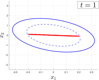
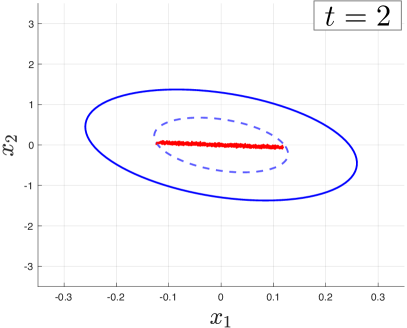
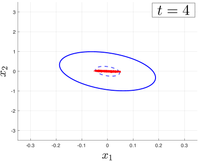
In this part, we use Proposition 1 to find probabilistic reachable sets of the inverted pendulum (7). We consider Assumption 2 with with positive definite matrix as defined above. For every , we have . Using Proposition 1 with the initial configuration , the probabilistic reachable sets of the stochastic system (7) with probability higher than or equal to are shown in Figure 1 (left).
Interval-based reachability
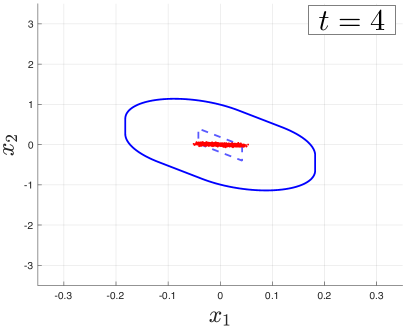
In this part, we use the separation strategy in Theorem 1 with the bounds on propagation of stochastic uncertainty obtained from Theorem 2 and the over-approximations of reachable sets of the associated deterministic system (7) obtained using interval-based reachability via a coordinate transformation. We consider the coordinate transformation with nonsingular matrix for the associated deterministic system (7). The transformed system is given by
| (13) |
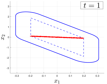
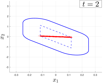
One can show that is a forward invariant set for the transformed system (13). Moreover, on the forward invariant set , an inclusion function for the transformed deterministic system (13) is given by . We denote the trajectory of the associated embedding system starting from by and use equation (9) to over-approximate the reachable sets of the transformed system (13). More specifically, at time , every trajectory of the transformed system (13) starting from belongs to the set . This implies that every trajectory of the associated deterministic system (7) starting from belongs to the parallelotope . The reachable sets of the system (7) with probability higher than or equal to obtained using separation strategy in Theorem 1 and interval-based reachability are shown in Figure 1 (right).
8 Conclusion
We developed a framework for reachability analysis of control systems with stochastic disturbances. A key feature of our framework is that it separates the effect of stochastic disturbances and deterministic inputs in the evolution of the system. We use contraction theory to obtain probabilistic bounds on propagation of stochastic disturbances and use the existing contraction-based and interval-based reachability frameworks to over-approximate the effect of deterministic input/disturbance. It is well-known that, for linear stochastic systems, the marginal distribution of trajectories is Gaussian and has an exponential tail [40, Section 6.2]. However, our results (Propositions 1 and 2) only imply sub-linearity of the marginal distribution of trajectories for linear stochastic systems. Future work will explore whether, for nonlinear stochastic systems, the marginal distributions of trajectories exhibit the same exponential tail behavior.
References
- [1] X. Chen and S. Sankaranarayanan, “Reachability analysis for cyber-physical systems: Are we there yet?” in NASA Formal Methods: 14th International Symposium, NFM 2022, Pasadena, CA, USA, May 24–27, 2022, Proceedings. Springer, 2022, pp. 109–130.
- [2] I. Mitchell, A. Bayen, and C. Tomlin, “A time-dependent Hamilton-Jacobi formulation of reachable sets for continuous dynamic games,” IEEE Transactions on Automatic Control, vol. 50, no. 7, pp. 947–957, 2005.
- [3] S. Bansal, M. Chen, S. Herbert, and C. J. Tomlin, “Hamilton-Jacobi reachability: A brief overview and recent advances,” in IEEE 56th Conference on Decision and Control (CDC), 2017, pp. 2242–2253.
- [4] A. B. Kurzhanski and P. Varaiya, “Ellipsoidal techniques for reachability analysis,” in Hybrid Systems: Computation and Control. Berlin, Heidelberg: Springer Berlin Heidelberg, 2000, pp. 202–214.
- [5] E. Asarin, O. Bournez, T. Dang, and O. Maler, “Approximate reachability analysis of piecewise-linear dynamical systems,” in Hybrid Systems: Computation and Control, 2000, pp. 20–31.
- [6] M. Althoff, O. Stursberg, and M. Buss, “Computing reachable sets of hybrid systems using a combination of zonotopes and polytopes,” Nonlinear Analysis: Hybrid Systems, vol. 4, no. 2, pp. 233–249, 2010, iFAC World Congress 2008.
- [7] S. Bak, H.-D. Tran, and T. T. Johnson, “Numerical verification of affine systems with up to a billion dimensions,” in Proceedings of the 22nd ACM International Conference on Hybrid Systems: Computation and Control, ser. HSCC ’19. New York, NY, USA: Association for Computing Machinery, 2019, p. 23–32.
- [8] Z. Huang and S. Mitra, “Computing bounded reach sets from sampled simulation traces,” in Hybrid Systems: Computation and Control, 2012, p. 291–294.
- [9] J. Maidens and M. Arcak, “Reachability analysis of nonlinear systems using matrix measures,” IEEE Transactions on Automatic Control, vol. 60, no. 1, pp. 265–270, 2015.
- [10] C. Fan, J. Kapinski, X. Jin, and S. Mitra, “Simulation-driven reachability using matrix measures,” ACM Transactions on Embedded Computing Systems, vol. 17, no. 1, dec 2017.
- [11] J. K. Scott and P. I. Barton, “Bounds on the reachable sets of nonlinear control systems,” Automatica, vol. 49, no. 1, pp. 93–100, 2013.
- [12] P.-J. Meyer, A. Devonport, and M. Arcak, “TIRA: Toolbox for interval reachability analysis,” in Proceedings of the 22nd ACM International Conference on Hybrid Systems: Computation and Control, 2019, pp. 224–229.
- [13] M. Abate, M. Dutreix, and S. Coogan, “Tight decomposition functions for continuous-time mixed-monotone systems with disturbances,” IEEE Control Systems Letters, vol. 5, no. 1, pp. 139–144, 2021.
- [14] S. Coogan, “Mixed monotonicity for reachability and safety in dynamical systems,” in 2020 59th IEEE Conference on Decision and Control (CDC), 2020, pp. 5074–5085.
- [15] H. M. Soner and N. Touzi, “Dynamic programming for stochastic target problems and geometric flows,” Journal of the European Mathematical Society, vol. 4, no. 3, pp. 201–236, 2002.
- [16] A. Abate, M. Prandini, J. Lygeros, and S. Sastry, “Probabilistic reachability and safety for controlled discrete time stochastic hybrid systems,” Automatica, vol. 44, no. 11, pp. 2724–2734, 2008.
- [17] P. Mohajerin Esfahani, D. Chatterjee, and J. Lygeros, “The stochastic reach-avoid problem and set characterization for diffusions,” Automatica, vol. 70, pp. 43–56, 2016.
- [18] A. P. Vinod and M. K. Oishi, “Stochastic reachability of a target tube: Theory and computation,” Automatica, vol. 125, p. 109458, 2021.
- [19] H. El-Samad, M. Fazel, X. Liu, A. Papachristodoulou, and S. Prajna, “Stochastic reachability analysis in complex biological networks,” in 2006 American Control Conference. IEEE, 2006, pp. 6–pp.
- [20] S. Prajna, A. Jadbabaie, and G. J. Pappas, “A framework for worst-case and stochastic safety verification using barrier certificates,” IEEE Transactions on Automatic Control, vol. 52, no. 8, pp. 1415–1428, 2007.
- [21] C. Santoyo, M. Dutreix, and S. Coogan, “A barrier function approach to finite-time stochastic system verification and control,” Automatica, vol. 125, p. 109439, 2021.
- [22] Q.-C. Pham, N. Tabareau, and J.-J. Slotine, “A contraction theory approach to stochastic incremental stability,” IEEE Transactions on Automatic Control, vol. 54, no. 4, pp. 816–820, 2009.
- [23] A. P. Dani, S.-J. Chung, and S. Hutchinson, “Observer design for stochastic nonlinear systems via contraction-based incremental stability,” IEEE Transactions on Automatic Control, vol. 60, no. 3, pp. 700–714, 2015.
- [24] H. Tsukamoto and S.-J. Chung, “Robust controller design for stochastic nonlinear systems via convex optimization,” IEEE Transactions on Automatic Control, vol. 66, no. 10, pp. 4731–4746, 2021.
- [25] C. Moore, “Unpredictability and undecidability in dynamical systems,” Physical Review Letters, vol. 64, pp. 2354–2357, May 1990.
- [26] A. Davydov, S. Jafarpour, and F. Bullo, “Non-euclidean contraction theory for robust nonlinear stability,” IEEE Transactions on Automatic Control, vol. 67, no. 12, pp. 6667–6681, 2022.
- [27] S. Jafarpour, A. Harapanahalli, and S. Coogan, “Efficient interaction-aware interval analysis of neural network feedback loops,” arXiv preprint, 2023. [Online]. Available: https://arxiv.org/abs/2307.14938
- [28] B. Øksendal, Stochastic differential equations: an introduction with applications, ser. Universitext. Springer Berlin, Heidelberg, 2013.
- [29] A. Devonport and M. Arcak, “Data-driven reachable set computation using adaptive gaussian process classification and monte carlo methods,” in 2020 American Control Conference (ACC), 2020, pp. 2629–2634.
- [30] T. Lew and M. Pavone, “Sampling-based reachability analysis: A random set theory approach with adversarial sampling,” in Conference on Robot Learning (CoRL). PMLR, 2021, pp. 2055–2070.
- [31] P. Gritzmann and B. Sturmfels, “Minkowski addition of polytopes: Computational complexity and applications to gröbner bases,” SIAM Journal on Discrete Mathematics, vol. 6, no. 2, pp. 246–269, 1993.
- [32] A. Halder, “On the parameterized computation of minimum volume outer ellipsoid of minkowski sum of ellipsoids,” in 2018 IEEE Conference on Decision and Control (CDC), 2018, pp. 4040–4045.
- [33] E. M. Aylward, P. A. Parrilo, and J.-J. E. Slotine, “Stability and robustness analysis of nonlinear systems via contraction metrics and sos programming,” Automatica, vol. 44, no. 8, pp. 2163–2170, 2008.
- [34] T. Lorenz, Mutational analysis: a joint framework for Cauchy problems in and beyond vector spaces, ser. Lecture Notes in Mathematics. Springer-Verlag, Berlin, 2010, vol. 1996.
- [35] R. Vershynin, High-Dimensional Probability: An Introduction with Applications in Data Science, ser. Cambridge Series in Statistical and Probabilistic Mathematics. Cambridge University Press, 2018.
- [36] W. Lohmiller and J.-J. E. Slotine, “On contraction analysis for non-linear systems,” Automatica, vol. 34, no. 6, pp. 683–696, 1998.
- [37] Z. Aminzare and E. D. Sontag, “Contraction methods for nonlinear systems: A brief introduction and some open problems,” in 53rd IEEE Conference on Decision and Control, 2014, pp. 3835–3847.
- [38] L. Jaulin, M. Kieffer, O. Didrit, and É. Walter, Applied Interval Analysis. Springer London, 2001.
- [39] A. Harapanahalli, S. Jafarpour, and S. Coogan, “A toolbox for fast interval arithmetic in numpy with an application to formal verification of neural network controlled system,” in 2nd ICML Workshop on Formal Verification of Machine Learning, 2023. [Online]. Available: https://arxiv.org/abs/2306.15340
- [40] S. Särkkä and A. Solin, Applied stochastic differential equations, ser. Institute of Mathematical Statistics Textbooks. Cambridge University Press, Cambridge, 2019, vol. 10.