Study of the mass of pseudoscalar glueball with a deep neural network

Abstract

A deep neural network (DNN) is utilized to study the mass of the pseudoscalar glueball in lattice QCD based on Monte Carlo simulations. To obtain an accurate and stable mass value, I constructed a new network. The results show that this DNN provides a more precise and stable mass estimate compared to the traditional least squares method.

I Introduction

Glueballs, the bound states of gluons predicted by Gell-Mann in 1962 [1], serve as a crucial element in Quantum Chromodynamics (QCD), where gluons act as the mediators of strong interactions, described by the SU(3) gauge fields $A_{\mu}(x)_{cd}$. Employing Euclidean spacetime, with Lorentz indices $\mu$ ranging from $\mu=1,2,3,4$, and color indices $c$ and $d$ spanning $c,d=1,2,3$, the gauge field $A_{\mu}(x)$ can be expressed as[2]

$$A_{\mu}(x)=\sum_{i=1}^{8}A_{\mu}^{i}(x)T_{i},$$ (1)

where $T_{i}$ are the generators of SU(3), and the resulting $A_{\mu}(x)$ are Hermitian and traceless matrices. In contrast to the single type of photon, mediating electromagnetic interactions in Quantum Electrodynamics, gluons exhibit eight types, each carrying color charge, thus engendering self-interactions and complicating the analysis of strong interactions.

Theoretically, several gluons can interact to form relatively stable bound states termed glueballs. These glueballs can be classified by their quantum numbers, including spin $J$, parity $P$, and charge conjugation $C$. For instance, the quantum numbers of a pseudoscalar glueball are denoted as $J^{PC}=0^{-+}$.

Understanding glueballs is crucial for deepening our comprehension of non-perturbative QCD effects and the confinement phenomenon.The exploration of glueballs offers profound insights into the non-perturbative domain of QCD. This paper aims to study the mass of pseudoscalar glueball. To achieve this, it is necessary to introduce the topological charge density[2]

$$q\left(x\right)=\frac{1}{32\pi^{2}}\varepsilon_{\mu\nu\rho\sigma}{\rm{Re}}{{\rm{Tr}}{\left[F_{\mu\nu}\left(x\right)F_{\rho\sigma}\left(x\right)\right]}},$$ (2)

where $F_{\mu\nu}(x)$ is the field strength tensor and the correlation function of $q(x)$ is as follows

$$C_{q}(r)=\langle q(x)q(y)\rangle,\quad r=|x-y|.$$ (3)

The correlation function $C_{q}(r)$ can be expressed as[3]

$$C_{q}(r)=\widetilde{C}_{q}(r)+B\delta^{4}(r).$$ (4)

Here, $\widetilde{C}_{q}(r)$ represents the negative tail of the correlation function $C_{q}(x-y)$ for $r>0$, and it can be used to extract the mass of the pseudoscalar glueball through the following relation

$$\widetilde{C}_{q}(r)=A\frac{m}{4\pi^{2}r}K_{1}(mr),$$ (5)

where $m$ is the pseudoscalar glueball mass, $A$ is an irrelevant normalization factor and $K_{1}$ is the modified Bessel function whose asymptotic form at large $|\arg z|$ is given by

$$K_{1}(z)\sim K_{1A}(z)=\sqrt{\frac{\pi}{2z}}\mathrm{e}^{-z}\left(1+\frac{3}{8z}\right),|\arg z|<\frac{3}{2}\pi.$$ (6)

In calculating the correlation function of the topological charge density, I need to use lattice QCD. Consequently, it is necessary to discretize certain physical quantities. In this paper, I choose the clover improved lattice discretization of the field strength tensor $F_{\mu\nu}\left(x\right)$ and it can be written as[2, 4]

$$\begin{array}[]{*{20}{c}}F_{\mu\nu}^{clov}(n)=-\frac{i}{8a^{2}}\left[\left(C_{\mu\nu}\left(n\right)-C_{\mu\nu}^{\dagger}(n)\right)-\frac{{\rm{Tr}}\left(C_{\mu\nu}\left(n\right)-C_{\mu\nu}^{\dagger}(n)\right)}{3}\right],\end{array}$$ (7)

where the clover is given as

$$C_{\mu\nu}(n)=U_{\mu,\nu}(n)+U_{\nu,-\mu}(n)+U_{-\mu,-\nu}(n)+U_{-\nu,\mu}(n).$$ (8)

The $U_{\mu v}\left(n\right)$ is the plaquette. After using lattice QCD to calculate $F_{\mu\nu}^{\text{clov}}(n)$, the correlation function $C_{q}(r_{n})$ and its negative tail $\widetilde{C}_{q}(r_{n})$ can be further obtained. $r_{n}$ is the discrete distance $r$.

On the other hand, machine learning(ML) is advancing the study of QCD. For instance, Generative Adversarial Networks can be used to reduce autocorrelation times in lattice QCD [5]. A Lattice gauge equivariant Convolutional Neural Network has been employed to approximate gauge covariant functions [6], and a modified Wasserstein generative adversarial network has been utilized to study topological quantities in lattice QCD [7].

In terms of function fitting, the traditional method of least squares(LS) is straightforward and computationally efficient. However, LS fitting is sensitive to outliers due to its reliance on the sum of squared deviations. This can significantly impact the overall fitting results, and it performs poorly in modeling complex nonlinear relationships. The process of fitting the mass of the pseudoscalar glueball involves complex nonlinear functions, thus posing limitations for the LS method. ML methods, on the other hand, have demonstrated excellent performance in fitting complex functions. Therefore, a Deep Neural Network (DNN) from ML is employed to fit the mass of the pseudoscalar glueball in this study, aiming to improve the fitting results.

II Data preparation

In this section, the aim is to obtain the correlation function data of the topological charge density $q(x)$. These data will be used for both traditional LS method and ML approach to determine the mass of the pseudoscalar glueball.

Firstly, the pseudo heat bath algorithm with periodic boundary conditions is employed to simulate lattice QCD configurations[2]. Subsequently, the Wilson flow is applied to smear these configurations[8]. The action employed here is the Wilson gauge action[2]

$${S_{G}}\left[U\right]=\frac{\beta}{3}\mathop{\sum}\limits_{n\in{\rm{\Lambda}}}\mathop{\sum}\limits_{\mu<\nu}{\mathop{\rm Re}\nolimits}{\rm{Tr}}\left[{1-{U_{\mu\nu}}\left(n\right)}\right],$$ (9)

where $\beta$ is the inverse coupling and $U_{\mu\nu}\left(n\right)$ is the plaquette. Configurations are generated using the software Chroma[9] on a personal workstation. Due to the high computational cost of computing the sum of the staples, the updating steps are repeated 10 times for the visited link variable. After the system reaches equilibrium, a total of 1000 configurations are sampled at intervals of 200 sweeps each. The integrated autocorrelation time for topological charge calculation is 0.416, indicating that each of data can be considered independent[7].

Furthermore, the static QCD potential is utilized to set the scale and can be parameterized by $V(r)=A+\frac{B}{r}+\sigma r$[2].The Sommer parameter $r_{0}$ is defined as

$$r_{0}^{2}\frac{dV(r)}{dr}\bigg{|}_{r=r_{0}}=1.65,$$ (10)

and $r_{0}=0.49$ fm is used[10]. The scale is shown in Tab. 1.

Table 1: The scale set through the static QCD potential.

$Volume$	$\beta$	$a[fm]$	$N_{cnfg}$	${r_{0}}/a$	$L[fm]$
$24\times{12}^{3}$	6.0	0.093(3)	1000	5.30(15)	1.11(3)

The lattice QCD configurations are further processed using Wilson flow [8]. The step size of the Wilson flow is set to $\varepsilon_{f}=0.01$. If the Wilson flow time $t_{f}$ is too large, it can lead to the elimination of negative part $\widetilde{C}_{q}(r_{n})$ of the correlation function $C_{q}(r_{n})$. Therefore, an appropriate Wilson flow time $t_{f}$ needs to be determined. In this paper, I adopt $\sqrt{8t_{f}}=0.15$ fm [11]. Subsequently, the smeared configurations are used to compute $C_{q}(r_{n})$.

III Machine learning model

III.1 Structure

DNN can assist in studying the mass of pseudoscalar glueball in lattice QCD. Tests have shown that when the structure of the DNN is too simple, the mass of the pseudoscalar glueball obtained from different amounts of data is inaccurate and unstable. Therefore, a more complex DNN was constructed. The structure of this DNN is illustrated in Fig. 1. This neural network employs 8 fully connected layers, each activated by a LeakyReLU function, except for the final layer, which uses a Sigmoid function. More specific parameters are detailed in the Tab. 2.

Figure 1: The structure of the DNN used to obtain the mass of the pseudoscalar glueball.

In the application phase, the inputs and outputs of the DNN are explained as follows. The input is a sequence $\left(c_{1},c_{2},\cdots,c_{N}\right)$ composed of the negative values $\widetilde{C}_{q}\left(r_{n}\right)$ of the correlation function calculated from lattice QCD at different positions. The value of $N$ varies for different lattice sizes, and in this paper, $N$ is 35. The output consists of two parameters, $P_{1}$ and $P_{2}$, both within the range (0, 1). The Sigmoid function in the last layer ensures that the output is within this range. These output parameters, $P_{1}$ and $P_{2}$, are proportional to the parameters $A$ and $m$ in $\widetilde{C}_{q}\left(r_{n}\right)$. Since the range of the DNN’s output is (0, 1), the mass $m$ of the pseudoscalar glueball needs to be scaled to fall within this range, corresponding to $P_{2}$. Because $aM$ is known to be a quantity between 0 and 2 [12], $aM/2$ becomes a quantity between 0 and 1. Thus, by scaling $M$ by $a/2$, it is adjusted to fall within the range of 0 to 1. Similarly, the parameter $A$ in $\widetilde{C}_{q}\left(r\right)$ is scaled accordingly. Therefore, the output parameter $P_{1}$ is proportional to the parameter $A$, and $P_{2}$ corresponds to $aM/2$. By obtaining the value of $aM/2$ from the DNN, the value of $M$ can be further determined. The detailed procedure on how the DNN is trained to ensure that $P_{1}$ and $P_{2}$ are proportional to the parameters $A$ and $m$ given the input $\left(c_{1},c_{2},\cdots,c_{N}\right)$ is elaborated in the training phase of the DNN.

The explanation for the parameter number in Tab. 2 is as follows. Taking Linear-1 as an example, the input to Linear-1 is a tensor with the shape $[-1,35]$, where $-1$ is a placeholder corresponding to the batch size. Linear-1 has 6400 neurons, and each neuron has a bias. Therefore, the Parameter number is calculated as $35\times 6400+6400=230400$.

Table 2: The structure of the DNN.

Layer (type)	Output Shape	Parameter number
Linear-1	[-1, 6400]	230,400
LeakyReLU-2	[-1, 6400]	0
Linear-3	[-1, 100]	640,100
LeakyReLU-4	[-1, 100]	0
Linear-5	[-1, 4]	404
LeakyReLU-6	[-1, 4]	0
Linear-7	[-1, 100]	500
LeakyReLU-8	[-1, 100]	0
Linear-9	[-1, 4]	404
LeakyReLU-10	[-1, 4]	0
Linear-11	[-1, 100]	500
LeakyReLU-12	[-1, 100]	0
Linear-13	[-1, 6400]	646,400
LeakyReLU-14	[-1, 6400]	0
Linear-15	[-1, 2]	12,802
Sigmoid-16	[-1, 2]	0

III.2 Training

To enable the neural network to accurately determine the mass of the pseudoscalar glueball, the following method was used to train the DNN. The training process is illustrated in Fig. 2. During the training phase, the following function was introduced

$$f(r_{n},l_{1},l_{2})=-\frac{50l_{1}l_{2}}{\pi^{2}ar_{n}}K_{1A}\left(\frac{2l_{2}r_{n}}{a}\right),$$ (11)

where $K_{1A}(z)$ is the asymptotic form of the modified Bessel function at large $|\arg z|$. Specifically, when $l_{1}=-A/100$ and $l_{2}=am/2$, it follows that $\widetilde{C}_{q}(r_{n})=f(r_{n},-A/100,am/2)$.

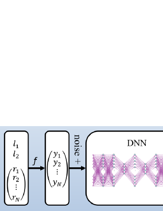
Figure 2: DNN training process.

For the preparation of the training data, two values were randomly selected from a uniform distribution between 0 and 1 as $l_{1}$ and $l_{2}$. These values, along with $r_{n}$, were then used to compute $y_{n}=f(r_{n},l_{1},l_{2})$, resulting in an array $\left(y_{1},y_{2},\cdots,y_{N}\right)$, to which noise was added. A total of 10,000 such processed arrays constituted the training dataset. From this dataset, arrays with batche size = 100 were selected and input into the DNN, which was trained to produce outputs $o_{1}$ and $o_{2}$ matching $l_{1}$ and $l_{2}$. Essentially, $l_{1}$ and $l_{2}$ serve as the labels for the arrays $\left(y_{1},y_{2},\cdots,y_{N}\right)$, and the goal of the DNN is to output the correct labels given the input arrays.

Since $\widetilde{C}_{q}(r_{n})$ can be considered a specific case of $f(r_{n},l_{1},l_{2})$, the DNN should be able to produce suitable outputs corresponding to $l_{1}$ and $l_{2}$, and consequently determine the parameters $A$ and the mass $m$, when given the $\widetilde{C}_{q}(r_{n})$ data computed from lattice QCD.

The optimizer used is Adam, proposed by Kingma and Ba [13], which combines the advantages of adaptive learning rates and momentum. Adam is chosen as the appropriate optimizer in this study due to its low memory requirements, automatic adjustment of learning rates, and ability to keep the step sizes within a general range.The loss function used in this paper is Binary Cross Entropy. Additionally, some programs are implemented using PyTorch [14].

IV Result

First, the correlation function of the topological charge density calculated by the Monte Carlo method with Wilson flow is presented. As shown in Fig. 3, it can be observed that the curve of the correlation function rises sharply as $r$ approaches 0. This behavior is consistent with the properties of $B\delta^{4}(r)$ in $C_{q}(r)$. In the region where $r$ is relatively large, the value of the correlation function increases with $r$ and gradually approaches 0 from negative values, aligning with the characteristics of the negative part $\widetilde{C}_{q}(r)$ in $C_{q}(r)$.

Figure 3: The curve of the correlation function $C_{q}\left(r\right)$ with $\sqrt{8t_{f}}=0.15\,\mathrm{fm}$.

For the LS method, I simulated a total of 1000 configurations and calculated the correlation function $C_{q}\left(r_{n}\right)$ from these configurations. Then the mass of the pseudoscalar glueball m=2370(92)MeV was fitted from 1000 ${\widetilde{C}}_{q}\left(r_{n}\right)$ data and details of the calculations are shown in Tab. 4, when 25 CPU cores were used in calculations.

For the DNN, models were trained with both noisy and noise-free training data. These models were then applied to $\widetilde{C}_{q}(r_{n})$ with different amounts of data to determine the mass of the pseudoscalar glueball. As shown in Fig. 4, the model trained with noisy data performed more accurately in obtaining the mass of the pseudoscalar glueball. For 1000 $\widetilde{C}_{q}(r_{n})$ data, the model trained with noisy yielded a mass of $m=2394(81)MeV$, which is consistent with results obtained by other researchers[12].

In terms of data details, I calculated the negative part $\widetilde{C}_{q}(r_{n})$ of the correlation function for every ten configurations, forming sequences $(c_{1},c_{2},\cdots,c_{N})$ at different distances $r_{n}$. Traditional LS method and ML method were then used to determine the mass of the pseudoscalar glueball, with errors handled using the jackknife method. The results are shown in Tab. 3.

Figure 4: The mass of the pseudoscalar glueball obtained by DNN models trained on datasets with and without noise, across varying data volumes of $\widetilde{C}_{q}(r_{n})$.

The important thing in the study is the accuracy of the physics results for LS and DNN. It can be observed from Tab.3 and Fig. 5 that the data error gradually decreases as the volume of data increases for both LS and DNN.In cases with the same amount of data, ML yields smaller errors in determining the mass of the pseudoscalar glueball compared to the LS. Furthermore, the fitting results obtained by ML are more stable across different data volumes. In cases with small data volume, the mass obtained by the LS is inaccurate. In contrast, the DNN can still produce good result even with small data volume.

Table 3: The mass $m$ of the pseudoscalar glueball obtained using the traditional LS method and the ML method.

Data volume	$m(LS)/MeV$	$m(ML)/MeV$
300	2238(169)	2379(144)
400	2177(136)	2351(120)
500	2234(123)	2388(110)
600	2264(114)	2388(102)
700	2283(106)	2357(95)
800	2330(103)	2376(91)
900	2338(98)	2379(85)
1000	2370(92)	2394(81)

Figure 5: The mass of the pseudoscalar glueball obtained using the traditional LS method and the ML approach under different data volumes

One possible explanation for these results is as follows. Fully connected layers in this DNN, by connecting all input units, can learn the global features of the input data. Despite the presence of noise in the data, the fully connected layers can still identify useful patterns. During training, the network adjusts its weights to fit the effective patterns in the data while ignoring the noisy features as much as possible. The stacking of multiple fully connected layers enhances the network’s nonlinear representation capability, allowing it to differentiate useful features from noise to some extent. Through this multi-layer structure, the network can extract higher-level features layer by layer, which helps to filter out the impact of noise at higher levels. Therefore, DNNs can suppress the influence of noise and extract effective features from the data to a certain degree. Related research also shows that DNNs can filter out noise in the data[15]. In contrast, the LS method determines model parameters by minimizing the sum of the squared errors between the original data and the predicted data, which makes it more susceptible to the impact of noise when the data volume is small, leading to instability in the results.

V Conclusion

This paper explores the mass of the pseudoscalar glueball using a DNN, showcasing the potential applications of ML method in lattice QCD. The findings from this study yield the following conclusions.

I designed a sophisticated DNN model for the study. The model trained with noisy data outperforms its noise-free counterpart in determining the pseudoscalar glueball mass, demonstrating its effectiveness. Across varying quantities of $\widetilde{C}_{q}(r_{n})$, the DNN model trained with noise consistently yields more precise results.

Furthermore, compared to traditional least squares method, this DNN model offers more accurate and stable estimate of the pseudoscalar glueball mass, particularly evident when considering different data quantities. For $\widetilde{C}_{q}(r_{n})$ data with a quantity of 1000, the DNN yields a mass estimation of 2394(81) MeV.

Ultimately, the application of machine learning in lattice QCD offers promising avenues for addressing various physics problems with increased precision in future studies.

Acknowledgments. This research utilized Chroma for simulating the lattice gauge field configurations. I extend my gratitude to the contributors of Chroma for their valuable contributions.

References

- Gell-Mann [1962] M. Gell-Mann, Phys. Rev. 125, 1067 (1962).
- Gattringer and Lang [2010] C. Gattringer and C. B. Lang, Quantum chromodynamics on the lattice, Vol. 788 (Springer, Berlin, 2010).
- Shuryak and Verbaarschot [1995] E. V. Shuryak and J. Verbaarschot, Physical Review D 52, 295 (1995).
- Wilson [1974] K. G. Wilson, Phys. Rev. D 10, 2445 (1974).
- Pawlowski and Urban [2020] J. M. Pawlowski and J. M. Urban, Machine Learning: Science and Technology 1, 045011 (2020).
- Favoni et al. [2022] M. Favoni, A. Ipp, D. I. Müller, and D. Schuh, Phys. Rev. Lett. 128, 032003 (2022).
- Gao et al. [2024] L. Gao, H. Ying, and J. Zhang, Physical Review D 109, 074509 (2024).
- Lüscher [2010] M. Lüscher, Journal of High Energy Physics 2010, 10.1007/jhep08(2010)071 (2010).
- Edwards and Joó [2005] R. G. Edwards and B. Joó, Nuclear Physics B - Proceedings Supplements 140, 832 (2005).
- Sommer [2014] R. Sommer, PoS LATTICE 2013, 015 (2014).
- Mazur et al. [2020] L. Mazur, L. Altenkort, O. Kaczmarek, and H.-T. Shu, arXiv preprint arXiv:2001.11967 (2020).
- Ablikim et al. [2024] M. Ablikim, M. Achasov, P. Adlarson, X. Ai, R. Aliberti, A. Amoroso, M. An, Q. An, Y. Bai, O. Bakina, et al., Physical Review Letters 132, 181901 (2024).
- Kingma and Ba [2014] D. P. Kingma and J. Ba, arXiv preprint arXiv:1412.6980 (2014).
- Paszke et al. [2019] A. Paszke, S. Gross, F. Massa, A. Lerer, J. Bradbury, G. Chanan, T. Killeen, Z. Lin, N. Gimelshein, L. Antiga, et al., Advances in neural information processing systems 32 (2019).
- Kolbæk et al. [2018] M. Kolbæk, Z.-H. Tan, and J. Jensen, in 2018 IEEE International Conference on Acoustics, Speech and Signal Processing (ICASSP) (IEEE, 2018) pp. 5059–5063.