Using Multimodal Foundation Models and Clustering for Improved Style Ambiguity Loss
Abstract
Teaching text-to-image models to be creative involves using style ambiguity loss, which requires a pretrained classifier. In this work, we explore a new form of the style ambiguity training objective, used to approximate creativity, that does not require training a classifier or even a labeled dataset. We then train a diffusion model to maximize style ambiguity to imbue the diffusion model with creativity and find our new methods improve upon the traditional method, based on automated metrics for human judgment, while still maintaining creativity and novelty.
1 Introduction
With every new invention comes a new wave of possibilities. Humans have been making pictures since before recorded history, so its only natural that there would be interest in computational image generation. Artificially generating photographs that are indistinguishable from real ones has become so easy and effective that there is even concern over "deepfakes" being used for propaganda or illicit purposes (Pawelec, 2022). On the other hand, generating images that look like art is a slightly different problem. The exact mathematical properties of what constitutes "quality" art is not as easy to quantify as other tasks, like classification accuracy, prediction error or whether a question was answered correctly. While machines can very easily be trained to mimic a dataset, humans like to be surprised by novelty, without feeling like they are being exposed to total randomness. A breakthrough was the invention of the Creative Adversarial Network (Elgammal et al., 2017), which used a style ambiguity loss to train a network to generate images that could not be classified as belonging to a particular style. However, GANs have largely been superseded by diffusion models (Luo, 2022), due to their far better results. Additionally, the style ambiguity loss requires a pretrained classifier. Every set of styles or concepts requires training a classifier before even training a model to generate images. Furthermore, training a classifier requires that the dataset be labeled correctly, and manually labeling a dataset is often even more expensive and time-consuming than training a model. To circumvent these issues, we propose using a classifier that does not require any additional training and can be easily applied to any dataset, labeled or unlabeled. Our contributions are as follows:
-
•
We applied creative style ambiguity loss to diffusion models, which are easier to train and produce higher-quality images than GANs.
-
•
We developed versatile CLIP-based and K-Means-based creative style ambiguity losses that do not require training a separate GAN-based style classifier.
-
•
Empirically, we find our new creative style ambiguity loss can be used to tune a diffusion model to generate samples that are higher quality than the generated samples of a diffusion model trained with the pre-existing GAN-based style ambiguity loss
2 Related Work
2.1 Creativity
Creativity has been hard to define and quantify. Creative work has been formulated as work having novelty, in that it differs from other similar objects, and also utility, in that it still performs a function (Cropley, 2006). For example, a Corinthian column has elaborate, interesting, unexpected adornments (novelty) but still holds up a building (utility). A distinction can also be made between "P-creativity", where the work is novel to the creator, and "H-creativity" where the work is novel to everyone (Boden, 1990). Computational techniques to be creative include using genetic algorithms (DiPaola & Gabora, 2008), reconstructing artifacts from novel collections of attributes (Iqbal et al., 2016), and most relevantly to this work, using Generative Adversarial Networks (Elgammal et al., 2017) with a style ambiguity loss.
2.2 Computational Art
One of the first algorithmic approaches dates back to the 1970s with the now primitive AARON (McCorduck, 1991), which was initially only capable of drawing black and white sketches. Generative Adversarial Networks (Goodfellow et al., 2014), or GANs, were some of the first models to be able to create complex, photorealistic images and seemed to have potential to be able to make art. Despite many problems with GANs, such as mode collapse and unstable training (Saxena & Cao, 2023), GANs and further improvements (Arjovsky et al., 2017; Karras et al., 2019; 2018) were state of the art until the introduction of diffusion Sohl-Dickstein et al. (2015). Diffusion models such as IMAGEN (Saharia et al., 2022) and DALLE-3 (Betker et al., ) have attained widespread commercial success (and controversy) due to their widespread adoption.
2.3 Reinforcement Learning
Reinforcement learning (RL) is a method of training a model by having it take actions that generate a reward signal and change the environment, thus changing the impact and availability of future actions Qiang & Zhongli (2011). RL has been used for tasks as diverse as playing board games (Silver et al., 2017), protein design (Lutz et al., 2023), self-driving vehicles (Kiran et al., 2021) and quantitative finance (Sahu et al., 2023). Policy-gradient RL (Sutton et al., 1999) optimizes a policy that chooses which action to take at any given timestep, as opposed to value-based methods that may use a heuristic to determine the optimal choice. Examples of policy gradient methods include Soft Actor Critic (Haarnoja et al., 2018), Deep Deterministic Policy Gradient (Lillicrap et al., 2019) and Trust Region Policy Optimization (Schulman et al., 2017a).
3 Method
3.1 Model
3.1.1 Creative Adversarial Network
A Generative Adversarial Network, or GAN (Goodfellow et al., 2014), consists of two models, a generator and a discriminator. The generator generates samples from noise, and the discriminator detects if the samples are drawn from the real data or generated. During training, the generator is trained to trick the discriminator into classifying generated images as real, and the discriminator is trained to classify images correctly. Given a generator , a discriminator real images , and noise , the objective is:
At inference time, the generator is used to generate realistic samples. Elgammal et al. (2017) introduced the Creative Adversarial Network, or CAN, which was a DCGAN (Radford et al., 2016) where the discriminator was also trained to classify real samples, minimizing the style classification loss. Given classes of image (such as ukiyo-e, baroque, impressionism, etc.), the classification modules of the Discriminator that returns a probability distribution over the style classes for an image and the real labels , the style classification loss was:
Where CE is the cross entropy function.
The generator was also trained to generate samples that could not be easily classified as belonging to one class. This stylistic ambiguity is a proxy for creativity or novelty. Given a vector , where each entry , and some classifier the style ambiguity loss is:
The discriminator was additionally trained to minimize and the generator was additionally trained to minimize . In the original work, the authors set . For our work, we will be combining the Wasserstein and CAN methods. We used the following loss functions:
3.1.2 Diffusion
A diffusion model aims to learn to iteratively remove the noise from a corrupted sample to restore the original. Starting with , the forward process iteratively adds Gaussian noise to produce the noised version , using a noise schedule , which can be learned or manually set as a hyperparameter:
More importantly, we also want to model the reverse process , that turns a noisy sample back into , conditioned on some context . As is the fully noised version,
We train and via optimizing the variational lower bound of the negative likelihood of the data:
As shown by Ho et al. (2020), this is equivalent to estimating the noise at each step using a model . So the loss to be optimized is:
Once the model has been trained, the reverse process, aka inference, to generate a sample from noise can be done iteratively by finding given and or :
Acording to Ho et al. (2020), both versions of had similar results. In our case, we used .
A Variational Autoencoder (Kingma & Welling, 2022) consists of an encoder to map an image into a lower-dimensional latent space, and a decoder to reverse this process. Rombach et al. (2022) performs diffusion but uses the latent representation of images :
This method, which we employed in this work, is known as stable diffusion. The encoding and decoding between the image dimensions and the latent dimensions is often implicit, and for the rest of the paper we will use not , as is common in the literature.
3.1.3 Markov Decision Processes
A Markov Decision Process (Bellman, 1957) is defined as a tuple that models the actions of an agent in some environment with discrete time-steps.
-
is the state space, the set of states the environment can be in.
-
is the set of actions that the agent can take.
-
is the initial distributions of states when .
-
is the probability of transitioning from state at time to at when the agent has taken action .
-
The reward function returns a reward a time given the action the agent takes and the state of the environment .
The agents actions are determined by the policy that maps actions to states. The series of state-action pairs for each timestep is called a trajectory . Using policy-gradient as opposed to value-based RL, we train by maximizing the reward over the trajectories sampled from the policy:
3.1.4 Denoising Diffusion Proximal Optimisation
Introduced by Black et al. (2023), Denoising Diffusion Proximal Optimisation, or DDPO, represents the Diffusion Process as a Markov Decision Process. A similar method was also pursued by Fan et al. (2023).
Reinforcement learning training was then applied to a pretrained diffusion model, which in our case was Stable Diffusion 2 (Rombach et al., 2022). Following Schulman et al. (2017b), Black et al. (2023) also implemented clipping to protect the policy gradient from excessively large updates. We largely follow their method but use a different reward function. We fine-tune off of the pre-existing stabilityai/stable-diffusion-2-base checkpoint (Rombach et al., 2022) downloaded from https://huggingface.co/stabilityai/stable-diffusion-2-base.
3.2 Reward Function
In the original paper, the authors used four different reward functions for four different tasks. For example, they used a scorer trained on the LAION dataset (Schuhmann & Beaumont, 2022) as the reward function to improve the aesthetic quality of generated outputs. In this paper, we use the reward model based on Elgammal et al. (2017), where the model is rewarded for stylistic ambiguity. Given a generated image and a classifier we want to maximize:
where CE is the cross entropy.
3.3 Data
Starting with the WikiArt dataset (Saleh & Elgammal, 2015), we used 1000 images from each class, oversampling when necessary, to balance the distributions between classes, to train the CAN. To train the diffusion model, we prompted the model by concatenating a randomly selected medium prompt from (painting of , picture of , drawing of ) to a randomly selected subject prompt (a man, a woman, a landscape, nature, a building, an animal, shapes, an object). An example prompt would be picture of an animal. With 10% probability we would set the prompt to the null string in order to train the model unconditionally as well.
3.4 Choice of Classifier
Style ambiguity loss relies on some classifier . We are exploring four versions of this classifier.
3.4.1 DCGAN-Based Classifier
We can use the classification module of the discriminator as the classifier in the reward function, setting . In the case of the CAN, is trained jointly along with the generator. In the case of DDPO, we use a pretrained from the CAN discriminator (which we call Diffusion DCGAN Based).
3.4.2 CLIP-Based Classifier
Given text and an image ,we can use a pretrained CLIP (Radford et al., 2021) model, that can return a similarity score for each image-text pair: . CLIP is a multimodal foundation model trained using contrastive learning (Jaiswal et al., 2021) on a dataset of approximately 400 million text-image pairs. For each generated image , for each class name , we find . We can then create a vector and then use softmax to normalize the vector and define the result as . Formally:
Then we set . We discard the results of when using a CLIP-Based Classifier with CAN. We used the 27 style classes in the WikArt dataset (Saleh & Elgammal, 2015) as . A list of said classes can be found in Appendix A. We used the clip-vit-large-patch14 CLIP checkpoint downloaded from https://huggingface.co/openai/clip-vit-large-patch14.
3.4.3 K-Means Text and Image Based Classifiers
Alternatively, when we have text labels or source images, we can embed the labels or images into the CLIP embedding space and perform k-means clustering to generate k centers. Given a CLIP Embedder mapping images to embeddings, and the k centers we can create a vector and then use softmax to normalize the vector and define the result as . Formally:
Then we set . We used two sets of centers: one set from performing k-means clustering on the WikiArt images, which we called K Means Image Based, and one set from clustering the names of the 27 style classes, which we call K Means Text Based.
4 Results
We generated all images with width and height = 512. The authors used width and height = 256 in the original CAN paper. However, given that larger, more detailed images are preferred by most people, we thought it more relevant to focus on larger images. Refer to appendix C for results on smaller images and examples. Table 1 shows a few DDPO images with the prompts used to generate them. Appendix B shows more examples generated using different prompts.
| Prompt | CLIP Based | K Means Text | K Means Image | DCGAN |
|---|---|---|---|---|
| a painting of a man | ![[Uncaptioned image]](/html/2407.12009/assets/appendix-22-512/ddpo-clip-512_0.jpg) |
![[Uncaptioned image]](/html/2407.12009/assets/appendix-22-512/ddpo-kmeans-text-512_0.jpg) |
![[Uncaptioned image]](/html/2407.12009/assets/appendix-22-512/ddpo-kmeans-image-512_0.jpg) |
![[Uncaptioned image]](/html/2407.12009/assets/appendix-22-512/ddpo-dcgan-512_0.jpg) |
| a picture of a woman | ![[Uncaptioned image]](/html/2407.12009/assets/appendix-22-512/ddpo-clip-512_10.jpg) |
![[Uncaptioned image]](/html/2407.12009/assets/appendix-22-512/ddpo-kmeans-text-512_10.jpg) |
![[Uncaptioned image]](/html/2407.12009/assets/appendix-22-512/ddpo-kmeans-image-512_10.jpg) |
![[Uncaptioned image]](/html/2407.12009/assets/appendix-22-512/ddpo-dcgan-512_10.jpg) |
| a painting of an animal | ![[Uncaptioned image]](/html/2407.12009/assets/appendix-22-512/ddpo-clip-512_5.jpg) |
![[Uncaptioned image]](/html/2407.12009/assets/appendix-22-512/ddpo-kmeans-text-512_5.jpg) |
![[Uncaptioned image]](/html/2407.12009/assets/appendix-22-512/ddpo-kmeans-image-512_5.jpg) |
![[Uncaptioned image]](/html/2407.12009/assets/appendix-22-512/ddpo-dcgan-512_5.jpg) |
| a painting of nature | ![[Uncaptioned image]](/html/2407.12009/assets/appendix-22-512/ddpo-clip-512_3.jpg) |
![[Uncaptioned image]](/html/2407.12009/assets/appendix-22-512/ddpo-kmeans-text-512_3.jpg) |
![[Uncaptioned image]](/html/2407.12009/assets/appendix-22-512/ddpo-kmeans-image-512_3.jpg) |
![[Uncaptioned image]](/html/2407.12009/assets/appendix-22-512/ddpo-dcgan-512_3.jpg) |
| a drawing of a man | ![[Uncaptioned image]](/html/2407.12009/assets/appendix-22-512/ddpo-clip-512_18.jpg) |
![[Uncaptioned image]](/html/2407.12009/assets/appendix-22-512/ddpo-kmeans-text-512_18.jpg) |
![[Uncaptioned image]](/html/2407.12009/assets/appendix-22-512/ddpo-kmeans-image-512_18.jpg) |
![[Uncaptioned image]](/html/2407.12009/assets/appendix-22-512/ddpo-dcgan-512_18.jpg) |
| a drawing of a woman | ![[Uncaptioned image]](/html/2407.12009/assets/appendix-22-512/ddpo-clip-512_19.jpg) |
![[Uncaptioned image]](/html/2407.12009/assets/appendix-22-512/ddpo-kmeans-text-512_19.jpg) |
![[Uncaptioned image]](/html/2407.12009/assets/appendix-22-512/ddpo-kmeans-image-512_19.jpg) |
![[Uncaptioned image]](/html/2407.12009/assets/appendix-22-512/ddpo-dcgan-512_19.jpg) |
| (no prompt) | ![[Uncaptioned image]](/html/2407.12009/assets/appendix-22-512/ddpo-clip-512_8.jpg) |
![[Uncaptioned image]](/html/2407.12009/assets/appendix-22-512/ddpo-kmeans-text-512_8.jpg) |
![[Uncaptioned image]](/html/2407.12009/assets/appendix-22-512/ddpo-kmeans-image-512_8.jpg) |
![[Uncaptioned image]](/html/2407.12009/assets/appendix-22-512/ddpo-dcgan-512_8.jpg) |
4.1 Quantitative Evaluation
We generated 100 images using the same prompts the models were trained on for each model. We used three quantitative metrics to score the models
-
•
AVA Score: Consisting of CLIP+Multi-Layer Perceptron (Haykin, 2000), the AVA model was trained on the AVA dataset (Murray et al., 2016) of images and average rankings by human subjects, in order to learn to approximate human preferences given an image. We used the CLIP model weights from the clip-vit-large-patch14 checkpoint and the Multi-Layer Perceptron weights downloaded from https://huggingface.co/trl-lib/ddpo-aesthetic-predictor.
-
•
Image Reward: The image reward model (Xu et al., 2023) was trained to score images given their text description based on a dataset of images and human rankings. We used the image-reward python library found at https://github.com/THUDM/ImageReward/tree/main.
-
•
Prompt Similarity: Given the CLIP model’s ability to embed images and text into the same space, we can measure the similarity between an image and its source prompt by finding the cosine similarity between the two CLIP embeddings. We used the clip-vit-large-patch14 checkpoint.
| Model | AVA Score | Image Reward | Prompt Similarity |
|---|---|---|---|
| Diffusion- CLIP Based | 4.18 | -1.75 | 0.24 |
| Diffusion- K-Means Text Based | 4.60 | -1.21 | 0.26 |
| Diffusion- K-Means Image Based | 4.38 | -0.90 | 0.26 |
| Diffusion- DCGAN Based | 4.26 | -1.58 | 0.26 |
Results of our experiments are shown in table 2. The best scores are bolded. There was little variance in prompt similarity. However, both K-Means-based approaches improved upon the DCGAN-based approach in terms of the two metrics for human preferences, showing that our method improves upon the past work aesthetically while also circumventing the costly training time of using a CAN or needing a labeled dataset for training the style classifier component of the CAN.
4.2 Comparison with Baseline
It is worth contrasting our trained DDPO model with the default pretrained stabilityai/stable-diffusion-2-base checkpoint diffusion model we are fine-tuning (Rombach et al., 2022). This allows us to better visualize the difference the DDPO training with style ambiguity loss makes. We assumed that the DDPO images might be similar to the baseline model images generated with fewer steps, so we compared DDPO Images to the baseline using 30,15, and 10 inference steps, as seen in figure 3.
| Prompt | CLIP Based | K Means Text | K Means Image | DCGAN | Baseline (30 Steps) | Baseline (15 Steps) | Baseline (10 Steps) |
|---|---|---|---|---|---|---|---|
| a painting of a landscape | ![[Uncaptioned image]](/html/2407.12009/assets/comp-drawing-landscape/clip.jpg) |
![[Uncaptioned image]](/html/2407.12009/assets/comp-drawing-landscape/k-text.jpg) |
![[Uncaptioned image]](/html/2407.12009/assets/comp-drawing-landscape/k-image.jpg) |
![[Uncaptioned image]](/html/2407.12009/assets/comp-drawing-landscape/dcgan.jpg) |
![[Uncaptioned image]](/html/2407.12009/assets/comp-drawing-landscape/vanilla.jpg) |
![[Uncaptioned image]](/html/2407.12009/assets/comp-drawing-landscape/half.jpg) |
![[Uncaptioned image]](/html/2407.12009/assets/comp-drawing-landscape/third.jpg) |
| a picture of an animal | ![[Uncaptioned image]](/html/2407.12009/assets/comp-drawing-animal/clip.jpg) |
![[Uncaptioned image]](/html/2407.12009/assets/comp-drawing-animal/k-text.jpg) |
![[Uncaptioned image]](/html/2407.12009/assets/comp-drawing-animal/k-image.jpg) |
![[Uncaptioned image]](/html/2407.12009/assets/comp-drawing-animal/dcgan.jpg) |
![[Uncaptioned image]](/html/2407.12009/assets/comp-drawing-animal/vanilla.jpg) |
![[Uncaptioned image]](/html/2407.12009/assets/comp-drawing-animal/half.jpg) |
![[Uncaptioned image]](/html/2407.12009/assets/comp-drawing-animal/third.jpg) |
| a painting of a man | ![[Uncaptioned image]](/html/2407.12009/assets/comp-drawing-man/clip.jpg) |
![[Uncaptioned image]](/html/2407.12009/assets/comp-drawing-man/k-text.jpg) |
![[Uncaptioned image]](/html/2407.12009/assets/comp-drawing-man/k-image.jpg) |
![[Uncaptioned image]](/html/2407.12009/assets/comp-drawing-man/dcgan.jpg) |
![[Uncaptioned image]](/html/2407.12009/assets/comp-drawing-man/vanilla.jpg) |
![[Uncaptioned image]](/html/2407.12009/assets/comp-drawing-man/half.jpg) |
![[Uncaptioned image]](/html/2407.12009/assets/comp-drawing-man/third.jpg) |
In order to quantitatively compare our models to the baselines, we used the embedding of the [CLS] token from a vision transformer loaded from the dino-vits16 checkpoint (Caron et al., 2021) from https://huggingface.co/facebook/dino-vits16, as that encodes stylistic information (Tumanyan et al., 2022; Kwon & Ye, 2023). We averaged the cosine similarity between style embeddings of each pair of images , where was generated by the tuned model and was generated by the baseline model using 30,15 and 10 inference steps respectively, using the same prompt and initial random seed. We did this 40 times. Average style cosine similarities between the DDPO-trained models and the baselines are shown in table 4. A lower style cosine similarity implies that the diffusion model has learned to successfully "deviate" from the baseline. All diffusion models model were more similar to the 30-step baseline, which implies that the diffusion models are not just learning to generate blurrier, less precise samples, but were learning a new "style" of art.
| Baseline 30 Steps | Baseline 15 Steps | Baseline 10 Steps | |
|---|---|---|---|
| Diffusion- CLIP Based | 0.29 | 0.27 | 0.23 |
| Diffusion- K-Means Text Based | 0.29 | 0.28 | 0.25 |
| Diffusion- K-Means Image Based | 0.30 | 0.30 | 0.29 |
| Diffusion- DCGAN Based | 0.26 | 0.23 | 0.21 |
5 Conclusion
Training models with stylistic ambiguity loss teaches them to be creative. This work introduces new forms of stylistic ambiguity loss that do not require training a classifier or GAN, which can be time-consuming and unstable (Saxena & Cao, 2023). These new methods, particularly the K-Means-based approaches, scored higher than the traditional method on quantitative metrics of human judgement. Nonetheless, there are still more directions for this to go. Both the CLIP-based and K-Means Text-based style ambiguity losses require users to heuristically choose a set of styles to "deviate" from. In this work, we only used the 27 categories in the WikiArt dataset to be comparable to the original CAN paper. However, users may instead prefer a different set of styles or words, which may produce better or more interesting results. Additionally, the K-Means Image-based style ambiguity loss does not require a multimodal model like CLIP. We could have used any pretrained model to embed images into a lower-dimensional manifold, or trained a new one. Ergo, the K-means technique could be used for any medium, such as music (Elgammal, 2022; Zhang et al., 2023), new proteins (Winnifrith et al., 2023), stories (Mori et al., 2022) and videos (Cho et al., 2024).
Broader Impact Statement
Many are concerned about the impacts of generative AI. By making art, this work infringes upon a domain once exclusive to humans. Companies have faced scrutiny for possibly using AI (Gutierrez, 2024), and many creatives, such as screenwriters and actors, have voiced concerns about whether their jobs are safe (del Barco, 2023). Nonetheless, using AI can help humans by making them more efficient, providing inspiration, and generating ideas (Fortino, 2023; Campitiello, 2023; Darling, 2022). It’s also not certain how copyright protection will function for AI-generated art (Watiktinnakorn et al., 2023), given copyright law is based on the premise that creative works originate solely from human authorship. Clear, consistent policies, both at the government level and by industry and/or academic groups, will be needed to mitigate the harm and maximize the benefits for all members of society.
6 Assistance
Author Contributions
This work was done without any outside assistance or collaboration.
Acknowledgements
Rutgers Office of Advanced Research Computing kindly provided the computing infrastructure to run the experiments. A special thanks goes out to Dr. Ahmed Elgammal and Dr. Eugene White for their past advice prior to this work.
References
- Arjovsky et al. (2017) Martin Arjovsky, Soumith Chintala, and Léon Bottou. Wasserstein gan, 2017.
- Bellman (1957) Richard Bellman. A markovian decision process. Journal of Mathematics and Mechanics, 6(5):679–684, 1957. URL http://www.jstor.org/stable/24900506.
- (3) James Betker, Gabriel Goh, Li Jing, † TimBrooks, Jianfeng Wang, Linjie Li, † LongOuyang, † JuntangZhuang, † JoyceLee, † YufeiGuo, † WesamManassra, † PrafullaDhariwal, † CaseyChu, † YunxinJiao, and Aditya Ramesh. Improving image generation with better captions. URL https://api.semanticscholar.org/CorpusID:264403242.
- Black et al. (2023) Kevin Black, Michael Janner, Yilun Du, Ilya Kostrikov, and Sergey Levine. Training diffusion models with reinforcement learning, 2023.
- Boden (1990) Margaret Boden. The Creative Mind. Abacus, 1990.
- Campitiello (2023) Jess Campitiello. Ai vs. artist: The future of creativity, 2023. URL https://tech.cornell.edu/news/ai-vs-artist-the-future-of-creativity/.
- Caron et al. (2021) Mathilde Caron, Hugo Touvron, Ishan Misra, Hervé Jégou, Julien Mairal, Piotr Bojanowski, and Armand Joulin. Emerging properties in self-supervised vision transformers. In Proceedings of the International Conference on Computer Vision (ICCV), 2021.
- Cho et al. (2024) Joseph Cho, Fachrina Dewi Puspitasari, Sheng Zheng, Jingyao Zheng, Lik-Hang Lee, Tae-Ho Kim, Choong Seon Hong, and Chaoning Zhang. Sora as an agi world model? a complete survey on text-to-video generation, 2024.
- Cropley (2006) Arthur Cropley. In praise of convergent thinking. Creativity Research Journal, 18(3):391–404, 2006. doi: 10.1207/s15326934crj1803\_13. URL https://doi.org/10.1207/s15326934crj1803_13.
- Darling (2022) Kate Darling. Ai image generators will help artists, not replace them, 2022. URL https://www.sciencefocus.com/news/ai-image-generators-will-help-artists-not-replace-them.
- del Barco (2023) Mandalit del Barco. Some sag-aftra members are concerned about ai provisions in tentative deal, 2023. URL https://www.npr.org/2023/11/30/1216005659/some-sag-aftra-members-are-concerned-about-ai-provisions-in-tentative-deal.
- DiPaola & Gabora (2008) Steve DiPaola and Liane Gabora. Incorporating characteristics of human creativity into an evolutionary art algorithm. Genetic Programming and Evolvable Machines, 10(2):97–110, December 2008. ISSN 1573-7632. doi: 10.1007/s10710-008-9074-x. URL http://dx.doi.org/10.1007/s10710-008-9074-x.
- Dubey et al. (2022) Shiv Ram Dubey, Satish Kumar Singh, and Bidyut Baran Chaudhuri. Activation functions in deep learning: A comprehensive survey and benchmark, 2022.
- Dumoulin & Visin (2018) Vincent Dumoulin and Francesco Visin. A guide to convolution arithmetic for deep learning, 2018.
- Elgammal (2022) Ahmed Elgammal. Creative gan generating music deviating from style norms, Feb 2022.
- Elgammal et al. (2017) Ahmed M. Elgammal, Bingchen Liu, Mohamed Elhoseiny, and Marian Mazzone. CAN: creative adversarial networks, generating "art" by learning about styles and deviating from style norms. CoRR, abs/1706.07068, 2017. URL http://arxiv.org/abs/1706.07068.
- Fan et al. (2023) Ying Fan, Olivia Watkins, Yuqing Du, Hao Liu, Moonkyung Ryu, Craig Boutilier, Pieter Abbeel, Mohammad Ghavamzadeh, Kangwook Lee, and Kimin Lee. Dpok: Reinforcement learning for fine-tuning text-to-image diffusion models, 2023.
- Fortino (2023) Andres Fortino. Embracing creativity: How ai can enhance the creative process, 2023. URL https://www.sps.nyu.edu/homepage/emerging-technologies-collaborative/blog/2023/embracing-creativity-how-ai-can-enhance-the-creative-process.html.
- Goodfellow et al. (2014) Ian J. Goodfellow, Jean Pouget-Abadie, Mehdi Mirza, Bing Xu, David Warde-Farley, Sherjil Ozair, Aaron Courville, and Yoshua Bengio. Generative adversarial networks, 2014.
- Gugger et al. (2022) Sylvain Gugger, Lysandre Debut, Thomas Wolf, Philipp Schmid, Zachary Mueller, Sourab Mangrulkar, Marc Sun, and Benjamin Bossan. Accelerate: Training and inference at scale made simple, efficient and adaptable. https://github.com/huggingface/accelerate, 2022.
- Gutierrez (2024) Luis Joshua Gutierrez. Wizards of the coast repeats anti-ai stance, fights accusation against latest magic the gathering promo, 2024. URL https://www.gamespot.com/articles/wizards-of-the-coast-repeats-anti-ai-stance-fights-accusation-against-latest-magic-the-gathering-promo/1100-6520153/.
- Haarnoja et al. (2018) Tuomas Haarnoja, Aurick Zhou, Pieter Abbeel, and Sergey Levine. Soft actor-critic: Off-policy maximum entropy deep reinforcement learning with a stochastic actor, 2018.
- Haykin (2000) Simon Haykin. Neural networks: A guided tour. 2000.
- Ho et al. (2020) Jonathan Ho, Ajay Jain, and Pieter Abbeel. Denoising diffusion probabilistic models. CoRR, abs/2006.11239, 2020. URL https://arxiv.org/abs/2006.11239.
- Ioffe & Szegedy (2015) Sergey Ioffe and Christian Szegedy. Batch normalization: Accelerating deep network training by reducing internal covariate shift, 2015.
- Iqbal et al. (2016) Azlan Iqbal, Matej Guid, Simon Colton, Jana Krivec, Shazril Azman, and Boshra Haghighi. The digital synaptic neural substrate: A new approach to computational creativity, 2016.
- Jaiswal et al. (2021) Ashish Jaiswal, Ashwin Ramesh Babu, Mohammad Zaki Zadeh, Debapriya Banerjee, and Fillia Makedon. A survey on contrastive self-supervised learning, 2021.
- Karras et al. (2018) Tero Karras, Timo Aila, Samuli Laine, and Jaakko Lehtinen. Progressive growing of gans for improved quality, stability, and variation, 2018.
- Karras et al. (2019) Tero Karras, Samuli Laine, and Timo Aila. A style-based generator architecture for generative adversarial networks, 2019.
- Kingma & Welling (2022) Diederik P Kingma and Max Welling. Auto-encoding variational bayes, 2022.
- Kiran et al. (2021) B Ravi Kiran, Ibrahim Sobh, Victor Talpaert, Patrick Mannion, Ahmad A. Al Sallab, Senthil Yogamani, and Patrick Pérez. Deep reinforcement learning for autonomous driving: A survey, 2021.
- Kozodoi (2021) N Kozodoi. Gradient accumulation in pytorch, 2021.
- Kwon & Ye (2023) Gihyun Kwon and Jong Chul Ye. Diffusion-based image translation using disentangled style and content representation, 2023.
- Lacoste et al. (2019) Alexandre Lacoste, Alexandra Luccioni, Victor Schmidt, and Thomas Dandres. Quantifying the carbon emissions of machine learning, 2019.
- Lillicrap et al. (2019) Timothy P. Lillicrap, Jonathan J. Hunt, Alexander Pritzel, Nicolas Heess, Tom Erez, Yuval Tassa, David Silver, and Daan Wierstra. Continuous control with deep reinforcement learning, 2019.
- Luo (2022) Calvin Luo. Understanding diffusion models: A unified perspective, 2022.
- Lutz et al. (2023) Isaac D Lutz, Shunzhi Wang, Christoffer Norn, Alexis Courbet, Andrew J Borst, Yan Ting Zhao, Annie Dosey, Longxing Cao, Jinwei Xu, Elizabeth M Leaf, et al. Top-down design of protein architectures with reinforcement learning. Science, 380(6642):266–273, 2023.
- Maas et al. (2013) Andrew L Maas, Awni Y Hannun, Andrew Y Ng, et al. Rectifier nonlinearities improve neural network acoustic models. In Proc. icml, volume 30, pp. 3. Atlanta, GA, 2013.
- Mangrulkar et al. (2022) Sourab Mangrulkar, Sylvain Gugger, Lysandre Debut, Younes Belkada, Sayak Paul, and Benjamin Bossan. Peft: State-of-the-art parameter-efficient fine-tuning methods. https://github.com/huggingface/peft, 2022.
- McCorduck (1991) P. McCorduck. Aaron’s Code: Meta-art, Artificial Intelligence, and the Work of Harold Cohen. W.H. Freeman, 1991. ISBN 9780716721734. URL https://books.google.com/books?id=r3UyBgAAQBAJ.
- Mori et al. (2022) Yusuke Mori, Hiroaki Yamane, Yusuke Mukuta, and Tatsuya Harada. Computational storytelling and emotions: A survey, 2022.
- Murray et al. (2016) Naila Murray, Luca Marchesotti, and Florent Perronnin. Ava: A large-scale database for aesthetic visual analysis. 2016. URL https://github.com/imfing/ava_downloader.
- Paszke et al. (2017) Adam Paszke, Sam Gross, Soumith Chintala, Gregory Chanan, Edward Yang, Zachary DeVito, Zeming Lin, Alban Desmaison, Luca Antiga, and Adam Lerer. Automatic differentiation in pytorch. 2017.
- Pawelec (2022) Maria Pawelec. Deepfakes and democracy (theory): How synthetic audio-visual media for disinformation and hate speech threaten core democratic functions. Digital Society, 1, 09 2022. doi: 10.1007/s44206-022-00010-6.
- Pedregosa et al. (2011) Fabian Pedregosa, Gaël Varoquaux, Alexandre Gramfort, Vincent Michel, Bertrand Thirion, Olivier Grisel, Mathieu Blondel, Peter Prettenhofer, Ron Weiss, Vincent Dubourg, Jake Vanderplas, Alexandre Passos, David Cournapeau, Matthieu Brucher, Matthieu Perrot, and Édouard Duchesnay. Scikit-learn: Machine learning in python. Journal of Machine Learning Research, 12(85):2825–2830, 2011. URL http://jmlr.org/papers/v12/pedregosa11a.html.
- Qiang & Zhongli (2011) Wang Qiang and Zhan Zhongli. Reinforcement learning model, algorithms and its application. In 2011 International Conference on Mechatronic Science, Electric Engineering and Computer (MEC), pp. 1143–1146, 2011. doi: 10.1109/MEC.2011.6025669.
- Radford et al. (2016) Alec Radford, Luke Metz, and Soumith Chintala. Unsupervised representation learning with deep convolutional generative adversarial networks, 2016.
- Radford et al. (2021) Alec Radford, Jong Wook Kim, Chris Hallacy, Aditya Ramesh, Gabriel Goh, Sandhini Agarwal, Girish Sastry, Amanda Askell, Pamela Mishkin, Jack Clark, Gretchen Krueger, and Ilya Sutskever. Learning transferable visual models from natural language supervision, 2021.
- Rombach et al. (2022) Robin Rombach, Andreas Blattmann, Dominik Lorenz, Patrick Esser, and Björn Ommer. High-resolution image synthesis with latent diffusion models. In Proceedings of the IEEE/CVF Conference on Computer Vision and Pattern Recognition (CVPR), pp. 10684–10695, June 2022.
- Saharia et al. (2022) Chitwan Saharia, William Chan, Saurabh Saxena, Lala Li, Jay Whang, Emily Denton, Seyed Kamyar Seyed Ghasemipour, Burcu Karagol Ayan, S. Sara Mahdavi, Rapha Gontijo Lopes, Tim Salimans, Jonathan Ho, David J Fleet, and Mohammad Norouzi. Photorealistic text-to-image diffusion models with deep language understanding, 2022.
- Sahu et al. (2023) Santosh Kumar Sahu, Anil Mokhade, and Neeraj Dhanraj Bokde. An overview of machine learning, deep learning, and reinforcement learning-based techniques in quantitative finance: Recent progress and challenges. Applied Sciences, 13(3):1956, 2023.
- Saleh & Elgammal (2015) Babak Saleh and Ahmed M. Elgammal. Large-scale classification of fine-art paintings: Learning the right metric on the right feature. CoRR, abs/1505.00855, 2015. URL http://arxiv.org/abs/1505.00855.
- Saxena & Cao (2023) Divya Saxena and Jiannong Cao. Generative adversarial networks (gans survey): Challenges, solutions, and future directions, 2023.
- Schuhmann & Beaumont (2022) Christoph Schuhmann and Romain Beaumont, 2022. URL https://laion.ai/blog/laion-aesthetics/.
- Schulman et al. (2017a) John Schulman, Sergey Levine, Philipp Moritz, Michael I. Jordan, and Pieter Abbeel. Trust region policy optimization, 2017a.
- Schulman et al. (2017b) John Schulman, Filip Wolski, Prafulla Dhariwal, Alec Radford, and Oleg Klimov. Proximal policy optimization algorithms, 2017b.
- Silver et al. (2017) David Silver, Julian Schrittwieser, Karen Simonyan, Ioannis Antonoglou, Aja Huang, Arthur Guez, Thomas Hubert, Lucas baker, Matthew Lai, Adrian Bolton, Yutian Chen, Timothy P. Lillicrap, Fan Hui, L. Sifre, George van den Driessche, Thore Graepel, and Demis Hassabis. Mastering the game of go without human knowledge. Nature, 550:354–359, 2017. URL https://api.semanticscholar.org/CorpusID:205261034.
- Sohl-Dickstein et al. (2015) Jascha Sohl-Dickstein, Eric A. Weiss, Niru Maheswaranathan, and Surya Ganguli. Deep unsupervised learning using nonequilibrium thermodynamics. CoRR, abs/1503.03585, 2015. URL http://arxiv.org/abs/1503.03585.
- Sutton et al. (1999) Richard S Sutton, David McAllester, Satinder Singh, and Yishay Mansour. Policy gradient methods for reinforcement learning with function approximation. In S. Solla, T. Leen, and K. Müller (eds.), Advances in Neural Information Processing Systems, volume 12. MIT Press, 1999. URL https://proceedings.neurips.cc/paper_files/paper/1999/file/464d828b85b0bed98e80ade0a5c43b0f-Paper.pdf.
- Tumanyan et al. (2022) Narek Tumanyan, Omer Bar-Tal, Shai Bagon, and Tali Dekel. Splicing vit features for semantic appearance transfer, 2022.
- von Platen et al. (2022) Patrick von Platen, Suraj Patil, Anton Lozhkov, Pedro Cuenca, Nathan Lambert, Kashif Rasul, Mishig Davaadorj, Dhruv Nair, Sayak Paul, William Berman, Yiyi Xu, Steven Liu, and Thomas Wolf. Diffusers: State-of-the-art diffusion models. https://github.com/huggingface/diffusers, 2022.
- von Werra et al. (2020) Leandro von Werra, Younes Belkada, Lewis Tunstall, Edward Beeching, Tristan Thrush, Nathan Lambert, and Shengyi Huang. Trl: Transformer reinforcement learning. https://github.com/huggingface/trl, 2020.
- Watiktinnakorn et al. (2023) Chawinthorn Watiktinnakorn, Jirawat Seesai, and Chutisant Kerdvibulvech. Blurring the lines: how ai is redefining artistic ownership and copyright. Discover Artificial Intelligence, 3, 11 2023. doi: 10.1007/s44163-023-00088-y.
- Winnifrith et al. (2023) Adam Winnifrith, Carlos Outeiral, and Brian Hie. Generative artificial intelligence for de novo protein design, 2023.
- Xu et al. (2023) Jiazheng Xu, Xiao Liu, Yuchen Wu, Yuxuan Tong, Qinkai Li, Ming Ding, Jie Tang, and Yuxiao Dong. Imagereward: Learning and evaluating human preferences for text-to-image generation, 2023.
- Zhang et al. (2023) Chenshuang Zhang, Chaoning Zhang, Sheng Zheng, Mengchun Zhang, Maryam Qamar, Sung-Ho Bae, and In So Kweon. A survey on audio diffusion models: Text to speech synthesis and enhancement in generative ai, 2023.
Appendix A WikiArt Style Classes
The 27 WikiArt style classes are listed in table 5
| contemporary-realism | art-nouveau-modern | abstract-expressionism |
|---|---|---|
| northern-renaissance | mannerism-late-renaissance | early-renaissance |
| realism | action-painting | color-field-painting |
| pop-art | new-realism | pointillism |
| expressionism | analytical-cubism | symbolism |
| fauvism | minimalism | cubism |
| romanticism | ukiyo-e | high-renaissance |
| synthetic-cubism | baroque | post-impressionism |
| impressionism | rococo | na-ve-art-primitivism |
Appendix B Images
Additional text prompts and the corresponding generated images using the DDPO models can be seen in Figures 6 and 7.
| Prompt | CLIP Based | K Means Text | K Means Image | DCGAN |
|---|---|---|---|---|
| a painting of a man | ![[Uncaptioned image]](/html/2407.12009/assets/appendix-19-512/ddpo-clip-512_0.jpg) |
![[Uncaptioned image]](/html/2407.12009/assets/appendix-19-512/ddpo-kmeans-text-512_0.jpg) |
![[Uncaptioned image]](/html/2407.12009/assets/appendix-19-512/ddpo-kmeans-image-512_0.jpg) |
![[Uncaptioned image]](/html/2407.12009/assets/appendix-19-512/ddpo-dcgan-512_0.jpg) |
| a picture of a woman | ![[Uncaptioned image]](/html/2407.12009/assets/appendix-19-512/ddpo-clip-512_10.jpg) |
![[Uncaptioned image]](/html/2407.12009/assets/appendix-19-512/ddpo-kmeans-text-512_10.jpg) |
![[Uncaptioned image]](/html/2407.12009/assets/appendix-19-512/ddpo-kmeans-image-512_10.jpg) |
![[Uncaptioned image]](/html/2407.12009/assets/appendix-19-512/ddpo-dcgan-512_10.jpg) |
| a painting of an animal | ![[Uncaptioned image]](/html/2407.12009/assets/appendix-19-512/ddpo-clip-512_5.jpg) |
![[Uncaptioned image]](/html/2407.12009/assets/appendix-19-512/ddpo-kmeans-text-512_5.jpg) |
![[Uncaptioned image]](/html/2407.12009/assets/appendix-19-512/ddpo-kmeans-image-512_5.jpg) |
![[Uncaptioned image]](/html/2407.12009/assets/appendix-19-512/ddpo-dcgan-512_5.jpg) |
| a painting of nature | ![[Uncaptioned image]](/html/2407.12009/assets/appendix-19-512/ddpo-clip-512_3.jpg) |
![[Uncaptioned image]](/html/2407.12009/assets/appendix-19-512/ddpo-kmeans-text-512_3.jpg) |
![[Uncaptioned image]](/html/2407.12009/assets/appendix-19-512/ddpo-kmeans-image-512_3.jpg) |
![[Uncaptioned image]](/html/2407.12009/assets/appendix-19-512/ddpo-dcgan-512_3.jpg) |
| a drawing of a man | ![[Uncaptioned image]](/html/2407.12009/assets/appendix-19-512/ddpo-clip-512_18.jpg) |
![[Uncaptioned image]](/html/2407.12009/assets/appendix-19-512/ddpo-kmeans-text-512_18.jpg) |
![[Uncaptioned image]](/html/2407.12009/assets/appendix-19-512/ddpo-kmeans-image-512_18.jpg) |
![[Uncaptioned image]](/html/2407.12009/assets/appendix-19-512/ddpo-dcgan-512_18.jpg) |
| a drawing of a woman | ![[Uncaptioned image]](/html/2407.12009/assets/appendix-19-512/ddpo-clip-512_19.jpg) |
![[Uncaptioned image]](/html/2407.12009/assets/appendix-19-512/ddpo-kmeans-text-512_19.jpg) |
![[Uncaptioned image]](/html/2407.12009/assets/appendix-19-512/ddpo-kmeans-image-512_19.jpg) |
![[Uncaptioned image]](/html/2407.12009/assets/appendix-19-512/ddpo-dcgan-512_19.jpg) |
| (no prompt) | ![[Uncaptioned image]](/html/2407.12009/assets/appendix-19-512/ddpo-clip-512_8.jpg) |
![[Uncaptioned image]](/html/2407.12009/assets/appendix-19-512/ddpo-kmeans-text-512_8.jpg) |
![[Uncaptioned image]](/html/2407.12009/assets/appendix-19-512/ddpo-kmeans-image-512_8.jpg) |
![[Uncaptioned image]](/html/2407.12009/assets/appendix-19-512/ddpo-dcgan-512_8.jpg) |
| Prompt | CLIP Based | K Means Text | K Means Image | DCGAN |
|---|---|---|---|---|
| a painting of a man | ![[Uncaptioned image]](/html/2407.12009/assets/appendix-20-512/ddpo-clip-512_0.jpg) |
![[Uncaptioned image]](/html/2407.12009/assets/appendix-20-512/ddpo-kmeans-text-512_0.jpg) |
![[Uncaptioned image]](/html/2407.12009/assets/appendix-20-512/ddpo-kmeans-image-512_0.jpg) |
![[Uncaptioned image]](/html/2407.12009/assets/appendix-20-512/ddpo-dcgan-512_0.jpg) |
| a picture of a woman | ![[Uncaptioned image]](/html/2407.12009/assets/appendix-20-512/ddpo-clip-512_10.jpg) |
![[Uncaptioned image]](/html/2407.12009/assets/appendix-20-512/ddpo-kmeans-text-512_10.jpg) |
![[Uncaptioned image]](/html/2407.12009/assets/appendix-20-512/ddpo-kmeans-image-512_10.jpg) |
![[Uncaptioned image]](/html/2407.12009/assets/appendix-20-512/ddpo-dcgan-512_10.jpg) |
| a painting of an animal | ![[Uncaptioned image]](/html/2407.12009/assets/appendix-20-512/ddpo-clip-512_5.jpg) |
![[Uncaptioned image]](/html/2407.12009/assets/appendix-20-512/ddpo-kmeans-text-512_5.jpg) |
![[Uncaptioned image]](/html/2407.12009/assets/appendix-20-512/ddpo-kmeans-image-512_5.jpg) |
![[Uncaptioned image]](/html/2407.12009/assets/appendix-20-512/ddpo-dcgan-512_5.jpg) |
| a painting of nature | ![[Uncaptioned image]](/html/2407.12009/assets/appendix-20-512/ddpo-clip-512_3.jpg) |
![[Uncaptioned image]](/html/2407.12009/assets/appendix-20-512/ddpo-kmeans-text-512_3.jpg) |
![[Uncaptioned image]](/html/2407.12009/assets/appendix-20-512/ddpo-kmeans-image-512_3.jpg) |
![[Uncaptioned image]](/html/2407.12009/assets/appendix-20-512/ddpo-dcgan-512_3.jpg) |
| a drawing of a man | ![[Uncaptioned image]](/html/2407.12009/assets/appendix-20-512/ddpo-clip-512_18.jpg) |
![[Uncaptioned image]](/html/2407.12009/assets/appendix-20-512/ddpo-kmeans-text-512_18.jpg) |
![[Uncaptioned image]](/html/2407.12009/assets/appendix-20-512/ddpo-kmeans-image-512_18.jpg) |
![[Uncaptioned image]](/html/2407.12009/assets/appendix-20-512/ddpo-dcgan-512_18.jpg) |
| a drawing of a woman | ![[Uncaptioned image]](/html/2407.12009/assets/appendix-20-512/ddpo-clip-512_19.jpg) |
![[Uncaptioned image]](/html/2407.12009/assets/appendix-20-512/ddpo-kmeans-text-512_19.jpg) |
![[Uncaptioned image]](/html/2407.12009/assets/appendix-20-512/ddpo-kmeans-image-512_19.jpg) |
![[Uncaptioned image]](/html/2407.12009/assets/appendix-20-512/ddpo-dcgan-512_19.jpg) |
| (no prompt) | ![[Uncaptioned image]](/html/2407.12009/assets/appendix-20-512/ddpo-clip-512_8.jpg) |
![[Uncaptioned image]](/html/2407.12009/assets/appendix-20-512/ddpo-kmeans-text-512_8.jpg) |
![[Uncaptioned image]](/html/2407.12009/assets/appendix-20-512/ddpo-kmeans-image-512_8.jpg) |
![[Uncaptioned image]](/html/2407.12009/assets/appendix-20-512/ddpo-dcgan-512_8.jpg) |
Appendix C Lower Dimensional Images
All experiments and images portrayed were done using images of dimension 512. However, we also repeated the experiments using smaller images. We briefly illustrate some example images in tables 8, 9 and 10 as well as quantitative evaluations in tables 11, 12 and 13.
| Prompt | CLIP Based | K Means Text | K Means Image | DCGAN |
|---|---|---|---|---|
| a painting of a man | ![[Uncaptioned image]](/html/2407.12009/assets/appendix-19-256/ddpo-clip-256_0.jpg) |
![[Uncaptioned image]](/html/2407.12009/assets/appendix-19-256/ddpo-kmeans-text-256_0.jpg) |
![[Uncaptioned image]](/html/2407.12009/assets/appendix-19-256/ddpo-kmeans-image-256_0.jpg) |
![[Uncaptioned image]](/html/2407.12009/assets/appendix-19-256/ddpo-dcgan-256_0.jpg) |
| a picture of a woman | ![[Uncaptioned image]](/html/2407.12009/assets/appendix-19-256/ddpo-clip-256_10.jpg) |
![[Uncaptioned image]](/html/2407.12009/assets/appendix-19-256/ddpo-kmeans-text-256_10.jpg) |
![[Uncaptioned image]](/html/2407.12009/assets/appendix-19-256/ddpo-kmeans-image-256_10.jpg) |
![[Uncaptioned image]](/html/2407.12009/assets/appendix-19-256/ddpo-dcgan-256_10.jpg) |
| a painting of an animal | ![[Uncaptioned image]](/html/2407.12009/assets/appendix-19-256/ddpo-clip-256_5.jpg) |
![[Uncaptioned image]](/html/2407.12009/assets/appendix-19-256/ddpo-kmeans-text-256_5.jpg) |
![[Uncaptioned image]](/html/2407.12009/assets/appendix-19-256/ddpo-kmeans-image-256_5.jpg) |
![[Uncaptioned image]](/html/2407.12009/assets/appendix-19-256/ddpo-dcgan-256_5.jpg) |
| a painting of nature | ![[Uncaptioned image]](/html/2407.12009/assets/appendix-19-256/ddpo-clip-256_3.jpg) |
![[Uncaptioned image]](/html/2407.12009/assets/appendix-19-256/ddpo-kmeans-text-256_3.jpg) |
![[Uncaptioned image]](/html/2407.12009/assets/appendix-19-256/ddpo-kmeans-image-256_3.jpg) |
![[Uncaptioned image]](/html/2407.12009/assets/appendix-19-256/ddpo-dcgan-256_3.jpg) |
| a drawing of a man | ![[Uncaptioned image]](/html/2407.12009/assets/appendix-19-256/ddpo-clip-256_18.jpg) |
![[Uncaptioned image]](/html/2407.12009/assets/appendix-19-256/ddpo-kmeans-text-256_18.jpg) |
![[Uncaptioned image]](/html/2407.12009/assets/appendix-19-256/ddpo-kmeans-image-256_18.jpg) |
![[Uncaptioned image]](/html/2407.12009/assets/appendix-19-256/ddpo-dcgan-256_18.jpg) |
| a drawing of a woman | ![[Uncaptioned image]](/html/2407.12009/assets/appendix-19-256/ddpo-clip-256_19.jpg) |
![[Uncaptioned image]](/html/2407.12009/assets/appendix-19-256/ddpo-kmeans-text-256_19.jpg) |
![[Uncaptioned image]](/html/2407.12009/assets/appendix-19-256/ddpo-kmeans-image-256_19.jpg) |
![[Uncaptioned image]](/html/2407.12009/assets/appendix-19-256/ddpo-dcgan-256_19.jpg) |
| (no prompt) | ![[Uncaptioned image]](/html/2407.12009/assets/appendix-19-256/ddpo-clip-256_8.jpg) |
![[Uncaptioned image]](/html/2407.12009/assets/appendix-19-256/ddpo-kmeans-text-256_8.jpg) |
![[Uncaptioned image]](/html/2407.12009/assets/appendix-19-256/ddpo-kmeans-image-256_8.jpg) |
![[Uncaptioned image]](/html/2407.12009/assets/appendix-19-256/ddpo-dcgan-256_8.jpg) |
| Prompt | CLIP Based | K Means Text | K Means Image | DCGAN |
|---|---|---|---|---|
| a painting of a man | ![[Uncaptioned image]](/html/2407.12009/assets/appendix-19-128/ddpo-clip-128_0.jpg) |
![[Uncaptioned image]](/html/2407.12009/assets/appendix-19-128/ddpo-kmeans-text-128_0.jpg) |
![[Uncaptioned image]](/html/2407.12009/assets/appendix-19-128/ddpo-kmeans-image-128_0.jpg) |
![[Uncaptioned image]](/html/2407.12009/assets/appendix-19-128/ddpo-dcgan-128_0.jpg) |
| a picture of a woman | ![[Uncaptioned image]](/html/2407.12009/assets/appendix-19-128/ddpo-clip-128_10.jpg) |
![[Uncaptioned image]](/html/2407.12009/assets/appendix-19-128/ddpo-kmeans-text-128_10.jpg) |
![[Uncaptioned image]](/html/2407.12009/assets/appendix-19-128/ddpo-kmeans-image-128_10.jpg) |
![[Uncaptioned image]](/html/2407.12009/assets/appendix-19-128/ddpo-dcgan-128_10.jpg) |
| a painting of an animal | ![[Uncaptioned image]](/html/2407.12009/assets/appendix-19-128/ddpo-clip-128_5.jpg) |
![[Uncaptioned image]](/html/2407.12009/assets/appendix-19-128/ddpo-kmeans-text-128_5.jpg) |
![[Uncaptioned image]](/html/2407.12009/assets/appendix-19-128/ddpo-kmeans-image-128_5.jpg) |
![[Uncaptioned image]](/html/2407.12009/assets/appendix-19-128/ddpo-dcgan-128_5.jpg) |
| a painting of nature | ![[Uncaptioned image]](/html/2407.12009/assets/appendix-19-128/ddpo-clip-128_3.jpg) |
![[Uncaptioned image]](/html/2407.12009/assets/appendix-19-128/ddpo-kmeans-text-128_3.jpg) |
![[Uncaptioned image]](/html/2407.12009/assets/appendix-19-128/ddpo-kmeans-image-128_3.jpg) |
![[Uncaptioned image]](/html/2407.12009/assets/appendix-19-128/ddpo-dcgan-128_3.jpg) |
| a drawing of a man | ![[Uncaptioned image]](/html/2407.12009/assets/appendix-19-128/ddpo-clip-128_18.jpg) |
![[Uncaptioned image]](/html/2407.12009/assets/appendix-19-128/ddpo-kmeans-text-128_18.jpg) |
![[Uncaptioned image]](/html/2407.12009/assets/appendix-19-128/ddpo-kmeans-image-128_18.jpg) |
![[Uncaptioned image]](/html/2407.12009/assets/appendix-19-128/ddpo-dcgan-128_18.jpg) |
| a drawing of a woman | ![[Uncaptioned image]](/html/2407.12009/assets/appendix-19-128/ddpo-clip-128_19.jpg) |
![[Uncaptioned image]](/html/2407.12009/assets/appendix-19-128/ddpo-kmeans-text-128_19.jpg) |
![[Uncaptioned image]](/html/2407.12009/assets/appendix-19-128/ddpo-kmeans-image-128_19.jpg) |
![[Uncaptioned image]](/html/2407.12009/assets/appendix-19-128/ddpo-dcgan-128_19.jpg) |
| (no prompt) | ![[Uncaptioned image]](/html/2407.12009/assets/appendix-19-128/ddpo-clip-128_8.jpg) |
![[Uncaptioned image]](/html/2407.12009/assets/appendix-19-128/ddpo-kmeans-text-128_8.jpg) |
![[Uncaptioned image]](/html/2407.12009/assets/appendix-19-128/ddpo-kmeans-image-128_8.jpg) |
![[Uncaptioned image]](/html/2407.12009/assets/appendix-19-128/ddpo-dcgan-128_8.jpg) |
| Prompt | CLIP Based | K Means Text | K Means Image | DCGAN |
|---|---|---|---|---|
| a painting of a man | ![[Uncaptioned image]](/html/2407.12009/assets/appendix-19-64/ddpo-clip-64_0.jpg) |
![[Uncaptioned image]](/html/2407.12009/assets/appendix-19-64/ddpo-kmeans-text-64_0.jpg) |
![[Uncaptioned image]](/html/2407.12009/assets/appendix-19-64/ddpo-kmeans-image-64_0.jpg) |
![[Uncaptioned image]](/html/2407.12009/assets/appendix-19-64/ddpo-dcgan-64_0.jpg) |
| a picture of a woman | ![[Uncaptioned image]](/html/2407.12009/assets/appendix-19-64/ddpo-clip-64_10.jpg) |
![[Uncaptioned image]](/html/2407.12009/assets/appendix-19-64/ddpo-kmeans-text-64_10.jpg) |
![[Uncaptioned image]](/html/2407.12009/assets/appendix-19-64/ddpo-kmeans-image-64_10.jpg) |
![[Uncaptioned image]](/html/2407.12009/assets/appendix-19-64/ddpo-dcgan-64_10.jpg) |
| a painting of an animal | ![[Uncaptioned image]](/html/2407.12009/assets/appendix-19-64/ddpo-clip-64_5.jpg) |
![[Uncaptioned image]](/html/2407.12009/assets/appendix-19-64/ddpo-kmeans-text-64_5.jpg) |
![[Uncaptioned image]](/html/2407.12009/assets/appendix-19-64/ddpo-kmeans-image-64_5.jpg) |
![[Uncaptioned image]](/html/2407.12009/assets/appendix-19-64/ddpo-dcgan-64_5.jpg) |
| a painting of nature | ![[Uncaptioned image]](/html/2407.12009/assets/appendix-19-64/ddpo-clip-64_3.jpg) |
![[Uncaptioned image]](/html/2407.12009/assets/appendix-19-64/ddpo-kmeans-text-64_3.jpg) |
![[Uncaptioned image]](/html/2407.12009/assets/appendix-19-64/ddpo-kmeans-image-64_3.jpg) |
![[Uncaptioned image]](/html/2407.12009/assets/appendix-19-64/ddpo-dcgan-64_3.jpg) |
| a drawing of a man | ![[Uncaptioned image]](/html/2407.12009/assets/appendix-19-64/ddpo-clip-64_18.jpg) |
![[Uncaptioned image]](/html/2407.12009/assets/appendix-19-64/ddpo-kmeans-text-64_18.jpg) |
![[Uncaptioned image]](/html/2407.12009/assets/appendix-19-64/ddpo-kmeans-image-64_18.jpg) |
![[Uncaptioned image]](/html/2407.12009/assets/appendix-19-64/ddpo-dcgan-64_18.jpg) |
| a drawing of a woman | ![[Uncaptioned image]](/html/2407.12009/assets/appendix-19-64/ddpo-clip-64_19.jpg) |
![[Uncaptioned image]](/html/2407.12009/assets/appendix-19-64/ddpo-kmeans-text-64_19.jpg) |
![[Uncaptioned image]](/html/2407.12009/assets/appendix-19-64/ddpo-kmeans-image-64_19.jpg) |
![[Uncaptioned image]](/html/2407.12009/assets/appendix-19-64/ddpo-dcgan-64_19.jpg) |
| (no prompt) | ![[Uncaptioned image]](/html/2407.12009/assets/appendix-19-64/ddpo-clip-64_8.jpg) |
![[Uncaptioned image]](/html/2407.12009/assets/appendix-19-64/ddpo-kmeans-text-64_8.jpg) |
![[Uncaptioned image]](/html/2407.12009/assets/appendix-19-64/ddpo-kmeans-image-64_8.jpg) |
![[Uncaptioned image]](/html/2407.12009/assets/appendix-19-64/ddpo-dcgan-64_8.jpg) |
| Model | AVA Score | Image Reward | Prompt Alignment |
|---|---|---|---|
| Diffusion- CLIP Based | 4.83 | -0.42 | 0.27 |
| Diffusion- K-Means Text Based | 4.91 | -0.64 | 0.27 |
| Diffusion- K-Means Image Based | 4.91 | -0.44 | 0.28 |
| Diffusion- DCGAN Based | 4.95 | -0.33 | 0.27 |
| Model | AVA Score | Image Reward | Prompt Alignment |
|---|---|---|---|
| Diffusion- CLIP Based | 4.47 | -0.74 | 0.27 |
| Diffusion- K-Means Text Based | 4.77 | -0.37 | 0.28 |
| Diffusion- K-Means Image Based | 3.78 | -1.36 | 0.25 |
| Diffusion- DCGAN Based | 4.66 | -0.14 | 0.29 |
| Model | AVA Score | Image Reward | Prompt Alignment |
|---|---|---|---|
| Diffusion- CLIP Based | 4.21 | -1.44 | 0.26 |
| Diffusion- K-Means Text Based | 4.36 | -1.00 | 0.27 |
| Diffusion- K-Means Image Based | 4.38 | -1.55 | 0.26 |
| Diffusion- DCGAN Based | 4.62 | -0.22 | 0.28 |
Appendix D Training
For reproducibility and transparency, the hyperparameters are listed in table 14 and table 15. All experiments were implemented in Python, building the models in pytorch (Paszke et al., 2017) using accelerate (Gugger et al., 2022) for efficient training. The diffusion models also relied on the trl (von Werra et al., 2020), diffusers (von Platen et al., 2022) and peft (Mangrulkar et al., 2022) libraries. The K-Means clustering was done using the k means implementation from scikit-learn (Pedregosa et al., 2011). A repository containing all code can be found on github at https://github.com/jamesBaker361/clipcreate/tree/main. Each experiment was run using two NVIDIA A100 GPUs with 40 GB RAM. Training times and estimated carbon emissions (Lacoste et al., 2019) calculated with https://mlco2.github.io/impact#compute are shown in table 16.
| Hyperparameter | Value |
|---|---|
| Epochs | 50 |
| Effective Batch Size | 8 |
| Batches per Epoch | 32 |
| Inference Steps per Image | 30 |
| LORA Matrix Rank | 4 |
| LORA | 4 |
| Optimizer | AdamW |
| Learning Rate | 3e-4 |
| AdamW | 0.9 |
| AdamW | 0.99 |
| AdamW Weight decay | 1e-4 |
| AdamW | 1e-8 |
D.1 Batch Size
For all DDPO models, we used an effective batch size of 8. When generating images with height and width 64, 128, and 512, we set the batch size to 8 without using gradient accumulation (Kozodoi, 2021). Curiously, for images of height and width 256, using a batch size of 8 caused an error: RuntimeError: CUDA error: CUBLAS_STATUS_ALLOC_FAILED when calling cublasCreate(handle). Thus, we opted to use a batch size of 4 with 2 gradient accumulation steps, equivalent to an effective batch size of 8, which worked. In order to investigate this error, we tried training a DDPO model with a batch size of 8 on a slower CPU, which was allocated 64 GB of memory. On the CPU, the error disappeared. We conclude that the reason for this error is dependent on how exactly variables are allocated across GPUs, but a more thorough investigation is beyond the scope of this paper.
| Hyperparameter | Value |
|---|---|
| Epochs | 100 |
| Batch Size | 32 |
| Optimizer | Adam |
| Learning Rate | 0.001 |
| Adam | 0.9 |
| Adam | 0.99 |
| Adam Weight decay | 0.0 |
| Adam | 1e-8 |
| Noise Dim | 100 |
| Wasserstein | 10 |
| Leaky ReLU negative slope | 0.2 |
| Convolutional Kernel | 4 |
| Convolutional Stride | 2 |
| Transpose Convolutional Kernel | 4 |
| Transpose Convolutional Stride | 2 |
| Model | Hours | kgCO2 |
| CAN (Image Dim 512) | 121.39 | 13.11 |
| Diffusion- CLIP Based (Image Dim 512) | 22.75 | 2.46 |
| Diffusion- K-Means Text Based (Image Dim 512) | 21.50 | 2.32 |
| Diffusion- K-Means Image Based (Image Dim 512) | 21.50 | 2.32 |
| Diffusion- DCGAN Based (Image Dim 512) | 21.44 | 2.32 |
| CAN (Image Dim 256) | 72.94 | 7.88 |
| Diffusion- CLIP Based (Image Dim 256) | 11.2 | 1.21 |
| Diffusion- K-Means Text Based (Image Dim 256) | 17.25 | 1.86 |
| Diffusion- K-Means Image Based (Image Dim 256) | 12.67 | 1.37 |
| Diffusion- DCGAN Based (Image Dim 256) | 8.53 | 0.92 |
| CAN (Image Dim 128) | 66.14 | 7.15 |
| Diffusion- CLIP Based (Image Dim 128) | 7.05 | 0.76 |
| Diffusion- K-Means Text Based (Image Dim 128) | 6.40 | 0.69 |
| Diffusion- K-Means Image Based (Image Dim 128) | 6.65 | 0.72 |
| Diffusion- DCGAN Based (Image Dim 128) | 6.24 | 0.67 |
| CAN (Image Dim 64) | 83.33 | 9 |
| Diffusion- CLIP Based (Image Dim 64) | 7.30 | 0.79 |
| Diffusion- K-Means Text Based (Image Dim 64) | 6.85 | 0.74 |
| Diffusion- K-Means Image Based (Image Dim 64) | 6.55 | 0.71 |
| Diffusion- DCGAN Based (Image Dim 64) | 6.14 | 0.66 |
D.2 Architecture
For diffusion model training, the text encoder, autoencoder and unet were all loaded from https://huggingface.co/stabilityai/stable-diffusion-2-base. These model components were all frozen, but we added trainable LoRA weights to the cross-attention layers of the Unet. Parameter counts are shown in table 17. The diffusion model components used the same amount of parameters regardless of image size, but the generator and discriminator had more parameters as image size increased.
| Model Component | Total Parameters | Trainable Parameters | Percent Trainable |
| Text Encoder | 34,0387,840 | 0 | 0% |
| Autoencoder | 83,653,863 | 0 | 0% |
| UNet | 866,740,676 | 829,952 | 0.1% |
| Generator (Image Dim 64) | 47,336,960 | 47,336,960 | 100% |
| Discriminator (Image Dim 64) | 13,691,612 | 13,691,612 | 100% |
| Generator (Image Dim 128) | 47,855,360 | 47,855,360 | 100% |
| Discriminator (Image Dim 128) | 14,347,228 | 14,347,228 | 100% |
| Generator (Image Dim 256) | 47,983,488 | 47,983,488 | 100% |
| Discriminator (Image Dim 256) | 15,920,604 | 15,920,604 | 100% |
| Generator (Image Dim 512) | 48,014,784 | 48,014,784 | 100% |
| Discriminator (Image Dim 512) | 20,115,932 | 20,115,932 | 100% |
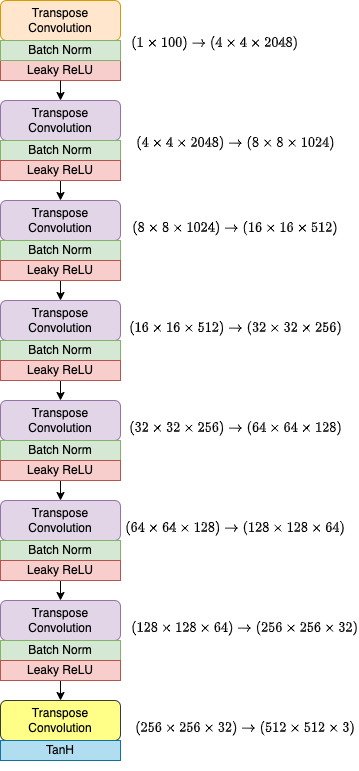
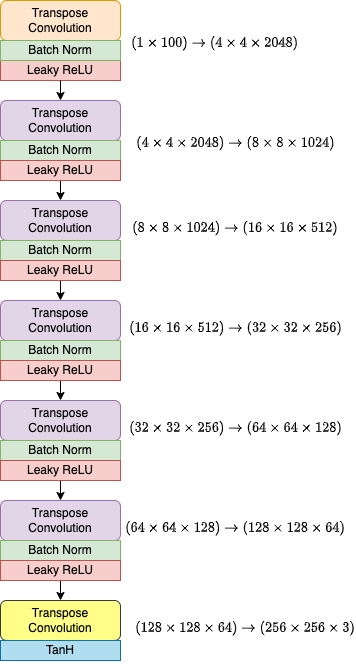
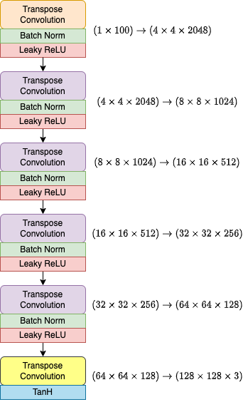
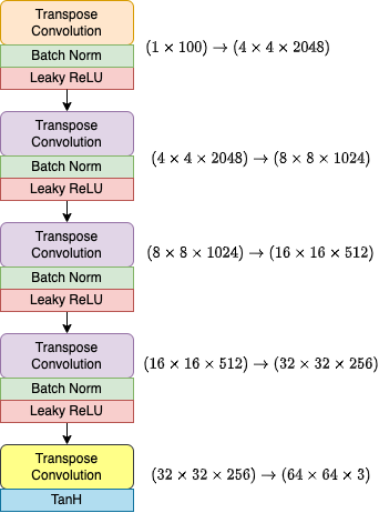
We used the convolutional neural network (Dumoulin & Visin, 2018) architecture described in Elgammal et al. (2017) for the CAN but had to use more/less layers to produce higher/lower dimension images. The generator takes a gaussian noise vector and maps it to a latent space, via a convolutional transpose layer with kernel size = 4 and stride =1, followed by 3, 4, 5 or 6 transpose convolutional layers corresponding to image dimensions 64, 128, 256 and 512, each upscaling the height and width dimensions by two, and halving the channel dimension (for example one of these transpose convolutional layers would map ) followed by batch normalization (Ioffe & Szegedy, 2015) and Leaky ReLU (Maas et al., 2013), and then one final convolutional transpose layer with output channels = 3 and tanh (Dubey et al., 2022) activation function. Diagrams of the generators with image dim 512, 256, 128 and 64 are shown in the figures 1, 2, 3 and 4 respectively.
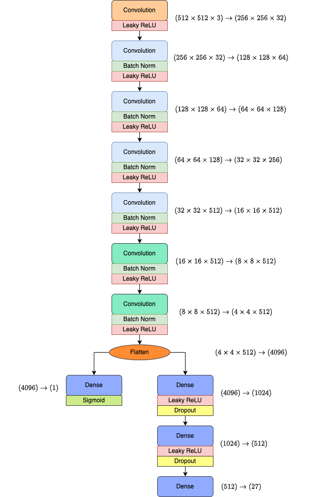
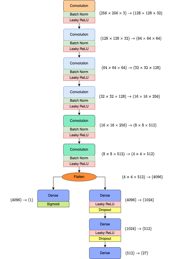
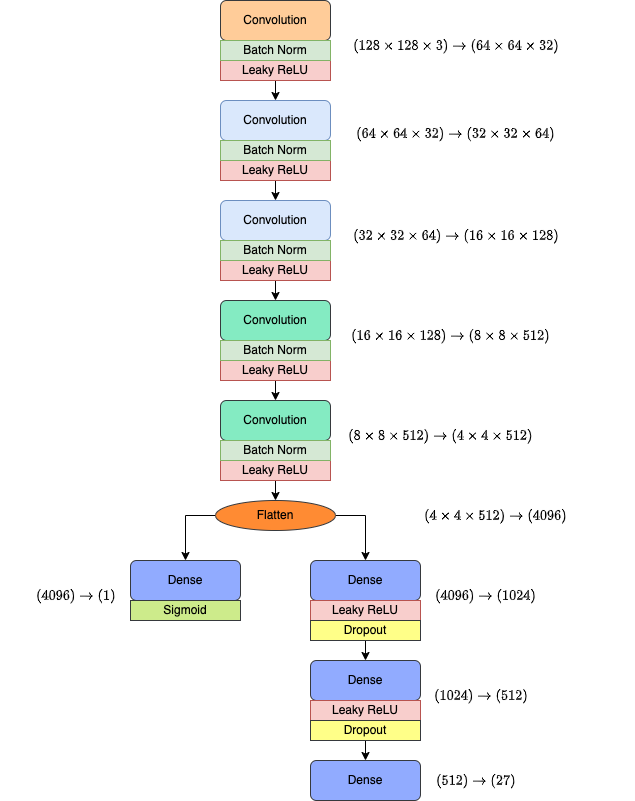
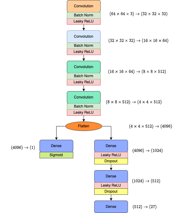
For the discriminator, we first applied a convolution layer to downscale the input image height width dimensions by 2 and mapped the 3 input channel dimensions to 32 () with Leaky ReLU activation. Then we had 2, 3, 4 or 5 convolutional layers corresponding to image dimensions 64, 128, 256 and 512, each downscaling the height and width dimensions by 2 and doubling the channel dimension (for example, one of these convolutional layers would map ) with batch normalization and Leaky ReLU activation. Then we had two more convolutional layers, each downscaling the height and width dimensions but keeping the channel dimensions constant (using the prior layer’s channel dimensions), with batch normalization and Leaky ReLU activation. The output of the convolutional layers was then flattened. The discriminator had two heads- one for style classification (determining which style a real image belongs to) and one for binary classification (determining whether an image was real or fake). The binary classification head consisted of one linear layer with one output neuron. The style classification layer consisted of 2 linear layers with LeakyReLU activation and Dropout, with output 1024 output neurons and 512 output neurons, respectively, followed by a linear layer with 27 output neurons for the 27 artistic style classes. Diagrams of discriminators with image dim 512, 256, 128, and 64 are shown in the figures 5, 6, 7, and 8, respectively.