Holographic QCD Running Coupling for Light Quarks in Strong Magnetic Field

Abstract

We consider running coupling constant in holographic model with external magnetic field supported by Einstein-dilaton-three-Maxwell action. We obtain a significant dependence of the running coupling constant $\alpha$ on chemical potential, temperature and magnetic field. We use the boundary condition that ensures the agreement with lattice calculations of string tension between quarks at zero chemical potential. The location of the 1-st order phase transitions in $(\mu,T)$-plane does not depend on the dilaton boundary conditions. We observe that running coupling $\alpha$ decreases with increasing magnetic field for the fixed values of chemical potential and temperature. At the 1-st order phase transitions the functions $\alpha$ undergo jumps depending on temperature, chemical potential and magnetic field.

1 Introduction

The goal of this paper is to study of the running coupling behavior in strong external magnetic field. This paper is the generalization of our consideration of running coupling in the isotropic holographic QCD [1] to anisotropic QCD [3, 2] originated by external magnetic field. We discuss here only the case of the light quarks model [2]. The running coupling in QCD can be found experimentally in wide range of energy. These data mainly concern the case of small density (small baryon chemical potential) available at LHC and RHIC. The last experimental data can be found in [4]. One can also compare the holographic results obtained in [1] with experimental data [5]; see also [6, 7, 8, 9] where holographic data obtained within other holographic models have been compared with experimental data. To obtain the dependence of the running coupling on the energy $E$ and the square of the transferred momenta $Q^{2}$, it is necessary to present a correspondence between them [6, 7, 8, 9]. In this research we investigated the dependence of the running coupling on the holographic coordinate $z$ that is related to the energy scale of QCD, corresponding to the warp factor.

In particular, it would be interesting to consider the holographic isotropic models of light and heavy quarks to study the running coupling as a function of the energy scale of QCD and try to fit the results of holographic models with experiments such as [7, 6]. The dilaton field plays a crucial role in the holographic approach to study the running coupling and it would be interesting to find out the effect of imposed proper boundary condition on the running coupling as a function of the energy scale of QCD for light and heavy quarks. In addition, in [8] considering holographic approach and using special form of Fourier transformation from ($z$ coordinate) 5-dimensional space-time in gravity side to the 4-dimensional one, the behavior of $\alpha$ as a function of momentum transfer, $Q^{2}$, is studied. We will apply this approach to our model in future studies. In this paper to obtain the dependence of the running coupling on the energy $E$ and the square of the transferred momenta $Q^{2}$, we use a simplest relation between them given by the prefactor in the 5-dimensional metric [6, 7, 5].

The QCD phase transition diagram in the (chemical potential, temperature) plane is both a challenging and significant topic in high-energy physics. This area of study is not only of fundamental interest but also has important implications for the early evolution of the Universe [10] and the interior of compact stellar objects [11, 12]. One of the primary goals of experiments at the LHC, RHIC, NICA, and FAIR is to explore the phase structure of strong-interaction matter under extreme conditions. Traditional theoretical methods for performing QCD calculations, such as perturbation theory, fail in the strongly coupled regime. Additionally, lattice theory faces a sign problem for non-zero chemical potential calculations and, at its current level, cannot provide adequate information. To describe the physics of the strongly coupled quark-gluon plasma (QGP) produced in heavy ion collisions (HIC) at RHIC, LHC, and NICA (see for example [13]), as well as in future experiments, non-perturbative approaches are required. Over the last three decades, holographic methods [14] have proven to be a powerful non-perturbative approach suitable for these purposes [15, 16, 17].

There are several experimental methods to study the QCD phase transition diagram. One of these methods is the Beam Energy Scan (BES) method [18, 19]. The BES method involves scanning a range of collision energies to search for signs of a 1-st order phase transition, such as changes in particle yields or the onset of collective phenomena. Nonmonotonic behavior in both beam energy and impact parameter dependences, if observed, can be used to identify such a phase transition.

Another method to identify the 1-st order phase transition is the study of strange particle production. Anomalies in the production of strange particles, such as kaons and hyperons, may signal the presence of a 1-st order phase transition [20]. Analyzing higher-order correlations and cumulants of particle distributions can provide evidence for critical phenomena associated with 1-st order phase transitions [21]. Finally, the measurement of elliptic flow as a function of collision energy can reveal changes in the medium’s properties, potentially indicating a 1-st order phase transition [22].

Here we would like to discuss another possibility. As shown in [1], Holographic QCD (HQCD) predicts discontinuities in the dependence of the running coupling on temperature $T$ and chemical potential $\mu$ akin to a 1-st order phase transition in the $(\mu,T)$-plane. From the positions of these discontinuities, one can predict the locations of 1-st-order phase transitions in the $(\mu,T)$-plane. Naturally, this necessitates access to high-density matter, specifically high chemical potentials, which may be attainable in future experiments such as NICA and FAIR.

During collisions of heavy ions, strong magnetic fields emerge, which subsequently influence the behavior of the running coupling constant. Therefore, it is crucial to assess the impact of strong magnetic fields on the running coupling in HQCD, or in other words, to determine how the results [1] are modified in the presence of a magnetic field. This constitutes the primary objective of this paper. As noted in [1], the structure of the QCD phase diagram is significantly influenced by the masses of the quarks. Here, for simplicity, we focus on the scenario involving light quarks.

The typical behavior of the running coupling $\alpha$, specifically the logarithm of the running coupling $\log\alpha$, as predicted by holographic models, has been presented in our paper [1]. This behavior is depicted at fixed energy scales, various temperatures, and chemical potentials, see also Fig.  4 below. A distinctive feature observed in different parts of this graph is the appearance of jumps in the coupling constant, indicating 1-st order phase transitions along the same lines in the ${\mu,T}$ planes, regardless of different values of energy scales. These jumps cease at the critical endpoint (CEP), marking the termination of the critical points’ lines. For non-zero magnetic fields, the 1-st order phase transition persists up to a certain value of the parameter $c_{B}$, as illustrated in Fig.  1 and Fig.  5.

The paper is organized as follows. In Sect. 2 we present 5-dim holographic models in the presence of non-zero magnetic field for light quarks. In Sect. 3 we describe the magnetic field influence on running coupling constant for the light quarks model. In Sect. 4 we summarize obtained results. The paper is supplemented by Appendix A, in which we briefly recall the basic facts about our holographic model.

2 Holographic model

Studying the effect of external magnetic field on the QCD features via holography are discussed in [3, 2, 23, 24, 25, 26, 27]. To investigate the behavior of the running coupling constant we use the holographic model for the light quarks in a magnetic field with the existence of 1-st order phase transition [2, 28]. For heavy quarks case the similar model has been proposed in [3]. These models generalize the corresponding isotropic models without magnetic fields [30, 29] and anisotropic ones with spacial anisotropy are related to the non-central HIC [31, 32, 26, 33, 34].

2.1 Black hole solution with three Maxwell fields

The 5-dimensional action in the Einstein frame has the following form [2]

$${\mathcal{S}}=\int\cfrac{d^{5}x\,\sqrt{-g}}{16\pi G_{5}}\left[R-\cfrac{f_{1}(\varphi)}{4}\ F_{(1)}^{2}-\cfrac{f_{2}(\varphi)}{4}\ F_{(2)}^{2}-\cfrac{f_{B}(\varphi)}{4}\ F_{(B)}^{2}-\cfrac{\partial_{\mu}\varphi\partial^{\mu}\varphi}{2}-V(\varphi)\right].$$ (2.1)

Here we use the ansatz, where the non-zero components of the electro-magnetic field and the field strengths are

$$A_{\mu}^{(1)}=A_{t}(z)\delta_{\mu}^{0},\quad F_{y_{1}y_{2}}^{(2)}=q,\quad F_{xy_{1}}^{(B)}=q_{B}.$$ (2.2)

In action (2.1) $R$ is Ricci scalar, $\varphi=\varphi(z)$ is the scalar field, $f_{1}(\varphi)$, $f_{2}(\varphi)$ and $f_{B}(\varphi)$ are the coupling functions associated with the Maxwell fields $A_{\mu}$, $F_{\mu\nu}^{(2)}$ and $F_{\mu\nu}^{(B)}$ correspondingly, $q$ and $q_{B}$ are constants and $V(\varphi)$ is the scalar field potential. Thus (2.1) is the extended version of the action used in [33, 31], where we add an external magnetic field $F_{\mu\nu}^{(B)}$.

We use the following ansatz for metric [2]:

$$ds^{2}=\cfrac{L^{2}\,\mathfrak{b}(z)}{z^{2}}\left[-\,g(z)dt^{2}+dx^{2}+\left(\cfrac{z}{L}\right)^{2-\frac{2}{\nu}}\!\!dy_{1}^{2}+e^{c_{B}z^{2}}\left(\cfrac{z}{L}\right)^{2-\frac{2}{\nu}}\!\!dy_{2}^{2}+\cfrac{dz^{2}}{g(z)}\right],$$ (2.3)

$$\mathfrak{b}(z)=e^{2{\mathcal{A}}(z)}.$$ (2.4)

Let us make some notes on the main parameters of the metric (2.3). The difference between “heavy quarks” and “light quarks” cases lies in the form of the scale factor ${\mathcal{A}}(z)$ in the warp factor. For the heavy quarks model see [26] and for simple choice of ${\mathcal{A}}(z)=-\,s\,z^{2}/4$ [33]. To get the “light quarks” case we follow [29] and assume ${\mathcal{A}}(z)=-\,a\ln(bz^{2}+1)$ where the parameters $a=4.046$ and $b=0.01613$ GeV² can be obtained by fitting with experimental data [29].

Here parameters $\nu$ and $c_{B}$ have the same meaning as in [3]. The primary anisotropy parameter $\nu$ describes non-equivalence between longitudinal and transversal directions. The isotropic case corresponds to $\nu=1$ (that we used in this paper), while $\nu=4.5$ reproduces the multiplicity of the charged particles production [32].

We refer to $c_{B}$ as to the magnetic field parameter that describes the non-centrality of the HIC. Although explicit relation of $c_{B}$ to the magnitude of the magnetic field is not established, there are considerations suggesting that $B^{2}=-\,c_{B}$ ${{GeV}^{2}}$ [25, 35, 36]. Therefore, we have $c_{B}\leq 0$ in all our calculations. Magnetic field parameter $c_{B}$ is an implicit function of the magnetic charge $q_{B}$ from the ansatz (2.2). However, we will not need the explicit form of this relation in what follows. In our model we have two independent parameters, i.e. $c_{B}$ and $q_{B}$ in the metric (2.4) and action (2.1), respectively. We usually set $q=q_{B}=1$ in our numerical calculations and vary $c_{B}$. The metric ansatz (2.3) also contains the blackening function $g(z)$ which has crucial effect to obtain the temperature and entropy of the black hole.

Applying the stationary action principle, we get the same equations of motion (EOM) [2, 28, 3]:

$$\begin{split}\varphi^{\prime\prime}&+\varphi^{\prime}\left(\cfrac{g^{\prime}}{g}+\cfrac{3\mathfrak{b}^{\prime}}{2\mathfrak{b}}-\cfrac{\nu+2}{\nu z}+c_{B}z\right)+\left(\cfrac{z}{L}\right)^{2}\cfrac{\partial f_{1}}{\partial\varphi}\ \cfrac{(A_{t}^{\prime})^{2}}{2\mathfrak{b}g}-\\ &-\left(\cfrac{L}{z}\right)^{2-\frac{4}{\nu}}\cfrac{\partial f_{2}}{\partial\varphi}\ \cfrac{q^{2}\ e^{-c_{B}z^{2}}}{2\mathfrak{b}g}\ -\left(\cfrac{z}{L}\right)^{\frac{2}{\nu}}\cfrac{\partial f_{B}}{\partial\varphi}\ \cfrac{q_{B}^{2}}{2\mathfrak{b}g}\ -\left(\cfrac{L}{z}\right)^{2}\cfrac{\mathfrak{b}}{g}\ \cfrac{\partial V}{\partial\varphi}=0,\end{split}$$ (2.5)

$$A_{t}^{\prime\prime}+A_{t}^{\prime}\left(\cfrac{\mathfrak{b}^{\prime}}{2\mathfrak{b}}+\cfrac{f_{1}^{\prime}}{f_{1}}+\cfrac{\nu-2}{\nu z}+c_{B}z\right)=0,$$ (2.6)

$$g^{\prime\prime}+g^{\prime}\left(\cfrac{3\mathfrak{b}^{\prime}}{2\mathfrak{b}}-\cfrac{\nu+2}{\nu z}+c_{B}z\right)-\left(\cfrac{z}{L}\right)^{2}\cfrac{f_{1}(A_{t}^{\prime})^{2}}{\mathfrak{b}}-\left(\cfrac{z}{L}\right)^{\frac{2}{\nu}}\cfrac{q_{B}^{2}\ f_{B}}{\mathfrak{b}}=0,$$ (2.7)

$$\mathfrak{b}^{\prime\prime}-\cfrac{3(\mathfrak{b}^{\prime})^{2}}{2\mathfrak{b}}+\cfrac{2\mathfrak{b}^{\prime}}{z}-\cfrac{4\mathfrak{b}}{3\nu z^{2}}\left(\cfrac{\nu-1}{\nu}+\left(1-\cfrac{3\nu}{2}\right)c_{B}z^{2}-\cfrac{\nu c_{B}^{2}z^{4}}{2}\right)+\cfrac{\mathfrak{b}\,(\varphi^{\prime})^{2}}{3}=0,$$ (2.8)

$$2g^{\prime}\ \cfrac{\nu-1}{\nu}+3g\ \cfrac{\nu-1}{\nu}\left(\cfrac{\mathfrak{b}^{\prime}}{\mathfrak{b}}-\cfrac{4\left(\nu+1\right)}{3\nu z}+\cfrac{2c_{B}z}{3}\right)+\left(\cfrac{L}{z}\right)^{1-\frac{4}{\nu}}\cfrac{L\,q^{2}\,e^{-c_{B}z^{2}}f_{2}}{\mathfrak{b}}=0,$$ (2.9)

$$\begin{split}2g^{\prime}\left(1-\cfrac{1}{\nu}+c_{B}z^{2}\right)&+3g\left[\Big{(}1-\cfrac{1}{\nu}+c_{B}z^{2}\Big{)}\left(\cfrac{\mathfrak{b}^{\prime}}{\mathfrak{b}}-\cfrac{4}{3\nu z}+\cfrac{2c_{B}z}{3}\right)-\cfrac{4\left(\nu-1\right)}{3\nu z}\right]+\\ &+\left(\cfrac{L}{z}\right)^{1-\frac{4}{\nu}}\cfrac{L\,q^{2}\,e^{-c_{B}z^{2}}\,f_{2}}{\mathfrak{b}}-\left(\cfrac{z}{L}\right)^{1+\frac{2}{\nu}}\cfrac{L\,q_{B}^{2}f_{B}}{\mathfrak{b}}=0,\end{split}$$ (2.10)

$$\begin{split}\cfrac{\mathfrak{b}^{\prime\prime}}{\mathfrak{b}}&+\cfrac{(\mathfrak{b}^{\prime})^{2}}{2\mathfrak{b}^{2}}+\cfrac{3\mathfrak{b}^{\prime}}{\mathfrak{b}}\left(\cfrac{g^{\prime}}{2g}-\cfrac{\nu+1}{\nu z}+\cfrac{2c_{B}z}{3}\right)-\cfrac{g^{\prime}}{3zg}\left(5+\cfrac{4}{\nu}-3c_{B}z^{2}\right)+\\ &+\cfrac{8}{3z^{2}}\left(1+\cfrac{3}{2\nu}+\cfrac{1}{2\nu^{2}}\right)-\cfrac{4c_{B}}{3}\left(1+\cfrac{3}{2\nu}-\cfrac{c_{B}z^{2}}{2}\right)+\cfrac{g^{\prime\prime}}{3g}+\cfrac{2}{3}\left(\cfrac{L}{z}\right)^{2}\cfrac{\mathfrak{b}V}{g}=0.\end{split}$$ (2.11)

Turning off the external magnetic field, i.e. putting $c_{B}=q_{B}=f_{B}=0$ into (2.5)–(2.11), we get the EOM from [31]. Normalizing to the AdS-radius, $L=1$, we get the EOM from [33]. Excluding special anisotropy, i.e. putting $\nu=1$ and $f_{2}=0$, we get the expressions that fully coincide with the EOM from [29, 30]. Thus (2.5)–(2.11) are universal anisotropic EOM, appropriate both for heavy and light quarks description, that include solution from [29, 30] as an isotropic limit. To solve the EOMs, We utilize the general form of the boundary conditions:

$$A_{t}(0)=\mu,\quad A_{t}(z_{h})=0,$$ (2.12)

$$g(0)=1,\quad g(z_{h})=0,$$ (2.13)

$$\varphi(z_{0})=0\,,$$ (2.14)

where $z_{0}=0$ corresponds to [29] and $z_{0}=z_{h}$ to [33]. The choice of the boundary condition for the scalar field was discussed in details in [31].

2.2 Thermodynamics and background phase transition

For the metric (2.3), the temperature and entropy for the light quarks model can be written as:

$$T=\cfrac{|g^{\prime}|}{4\pi}\,\Bigl{|}_{z=z_{h}},\qquad s=\left(\cfrac{L}{z_{h}}\right)^{1+\frac{2}{\nu}}\cfrac{e^{c_{B}z_{h}^{2}/2}}{4\left(1+bz_{h}^{2}\right)^{3a}}.$$ (2.15)

Then, the phase diagrams for light quarks model can be obtained via free energy consideration

$$F=-\int s\,dT=\int_{z_{h}}^{\infty}s\,T^{\prime}dz,$$ (2.16)

where we normalized the free energy to vanish at $z_{h}\to\infty$. The background phase transition curves become shorter with the magnetic field increasing (larger $c_{B}$ absolute values). Using free energy (2.16) phase diagram $(\mu,T)$-plane for light quarks model describing the isotropic case $c_{B}=0$ and anisotropic cases with different $c_{B}$ is obtained in Fig. 1. Since in this paper we concentrated on just two different cases, i.e. $c_{B}=0$ and $c_{B}=-0.05$ ${{GeV}^{2}}$. In the Fig. 1 the associated CEPs are marked with magenta stars.

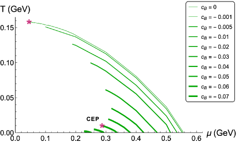
Figure 1: Phase diagram $(\mu,T)$-plane for light quarks model describing the isotropic case $c_{B}=0$ and anisotropic cases with different $c_{B}$. The magenta star indicates the CEP; $[c_{B}]=$ GeV²

The energy scale $E$ (GeV) as a function of the holographic coordinate $z$ (GeV^-1) corresponding to the prefactor of the metric (2.17) is defined as [7]:

$$E=\frac{\sqrt{\mathfrak{b}(z)}}{z}=\frac{\left(bz^{2}+1\right)^{-a}}{z}\,,$$ (2.17)

where parameters $a$ and $b$ were introduced in Sect. 2.1. The energy scale as a function of the holographic coordinate $E(z)$ is presented in Fig. 2

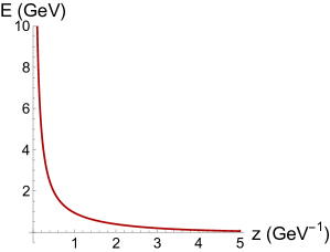
Figure 2: Energy scale $E$ (GeV) as a function of the holographic coordinate $z$ (GeV^-1) corresponding to the warp factor $\mathfrak{b}(z)$.

In Fig. 3 2D plots in $(\mu,z_{h})$-plane for $c_{B}=0$ (A) and $c_{B}=-0.05$ (B) are depicted. The magenta curves show coordinates of the 1-st order phase transition and the black contours correspond to the fixed temperatures and the brown one corresponds to the $T=0$. The magenta star is CEP. The magenta curves on each plot consist of two branches: the upper branch and the lower one are connected at the ”star” (CEP). These two branches are identified according to the same values of $\mu$ and $T$. The magenta lines indicate the size of the black holes horizons. Therefore, the regions of the stable black holes solutions are located above the upper magenta curve and below the lower branch. The area between the upper and lower branches of the magenta curves corresponds to the unstable region.

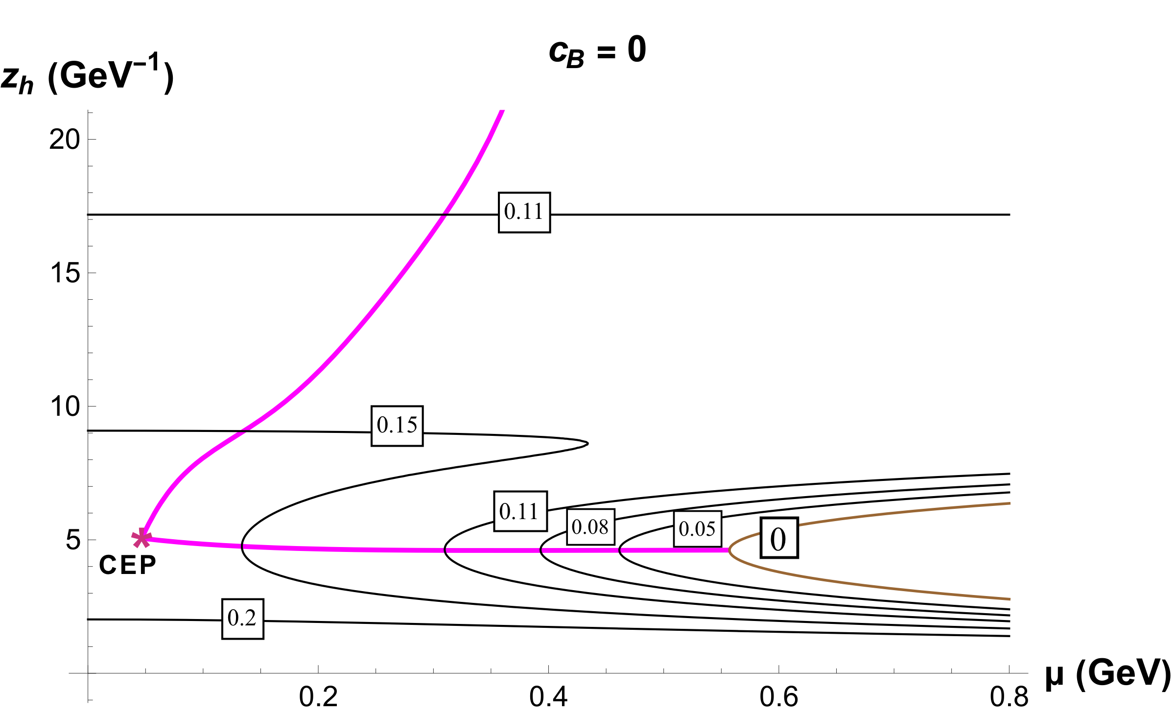
A
 

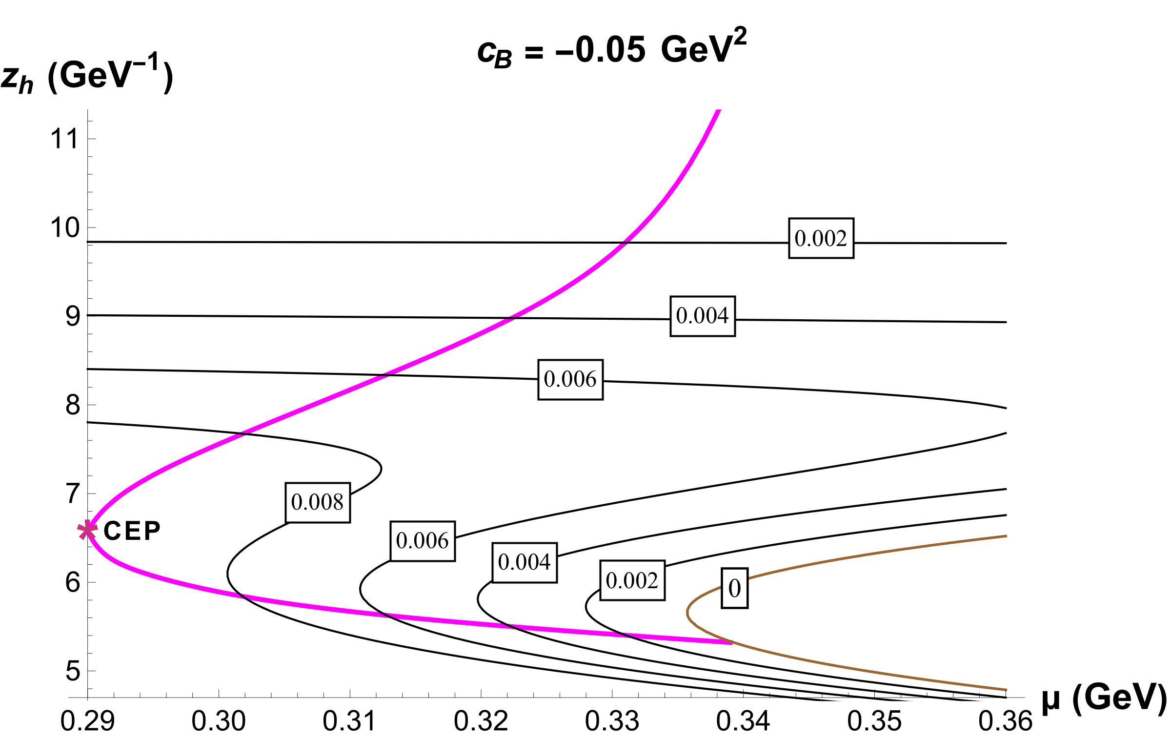
B

Figure 3: 2D plots in $(\mu,z_{h})$-plane for $c_{B}=0$ (A) and $c_{B}=-0.05$ GeV² (B). The magenta curves show coordinates of the 1-st order phase transition; the black contours correspond to the fixed temperatures and the brown one corresponds to the $T=0$. The magenta star is CEP; $[T]=$ GeV.

3 Running coupling in the strong magnetic field

The characteristic feature of the holographic coupling constant $\alpha$ is its dependence on the dilaton field and is defined as [37, 38, 6]

$$\alpha(z)=e^{\varphi(z)}\,.$$ (3.1)

The dilaton field $\varphi$ itself depends on the chosen boundary condition. We denote the dilaton field with the zero boundary condition at zero holographic coordinate as $\varphi=\varphi_{0}(z)$, i.e.

$$\varphi_{0}(z)\Big{|}_{z=0}=0.$$ (3.2)

The dilaton field with the boundary condition at the holographic coordinate $z=z_{0}$ is denoted by $\varphi_{z_{0}}(z)$. These two solutions are related by a simple relation

$$\varphi_{z_{0}}(z)=\varphi_{0}(z)-\varphi_{0}(z_{0}),$$ (3.3)

that gives

$$\alpha_{z_{0}}(z)=\alpha_{0}(z)\,\mathfrak{G}(z_{0}),\quad\qquad\alpha_{0}(z)=e^{\varphi_{0}(z)},\quad\mathfrak{G}(z_{0})=e^{-\varphi_{0}(z_{0})}$$ (3.4)

Note that $\varphi_{0}(z)$ does not depend on the thermodynamic characteristics of the model, see [1]. To obtain the dependence of the running coupling on thermodynamic quantities such as $T$ and $\mu$, one can take $z_{0}$ related with $z_{h}$, i.e. $z_{0}=\mathfrak{z}(z_{h})$, and get

$$\alpha_{\mathfrak{z}}(z;T,\mu)=\alpha_{0}(z)\,\mathfrak{G}(T,\mu),\qquad\quad\mathfrak{G}(T,\mu)=e^{-\varphi_{0}(\mathfrak{z}(z_{h}))}$$ (3.5)

One such choice is $\mathfrak{z}(z_{h})=z_{h}$, and the other is given by exponential function that is named as a second boundary condition at $z_{0}$ [1]:

$$z_{0}=\mathfrak{z}(z_{h})=10\,\exp(-\frac{z_{h}}{4})+0.1\,,$$ (3.6)

where dilaton field is zero at $z_{0}$, see (2.14). It is important to note the boundary condition (3.6) that introduced in [31] was obtained by studying the behavior of QCD string tension as a function of temperature at zero chemical potential for isotropic case acquired via lattice calculations [39]. This boundary condition (3.6) also is used in this research for anisotropic model, although there is no lattice results for the anisotropic $c_{B}\neq 0$ case.

To study the behavior of the running coupling constant for magnetic fields $c_{B}=0$ and $c_{B}=-0.05$ , we utilize the Fig. 3 to respect the physical regions of the model which is limited by the sizes of black holes, $z_{h}$, indicate a 1-st order phase transition.

In Fig. 4 density plots with contours for $\log\alpha_{\mathfrak{z}}(E;\mu,T)$ at different energy scales $E=\{0.5771,0.9373,1.9677\}$ (GeV) for $c_{B}=0$ are arranged in such a way that they represent a family of sections of three-dimensional space $(E,\mu,T)$. The selected values of energy scale $E$ correspond to holographic coordinate $z=\{0.5,\,1,\,1.5$} (GeV^-1) according to the Fig. 2. Each plot has several contours corresponding to fixed values of $\log\alpha_{\mathfrak{z}}$, these values are indicated in squares. The red lines in the first two graphs on the left indicate the maximum possible temperature values at the corresponding energy scale $E$. These restrictions arise due to the constraint $z\leq z_{h}$. The plot in Fig. 4 actually reproduces the plot presented earlier in the paper [1]. It can be seen that as we increase the energy scale, the contours of the fixed values of the running coupling constant go down to lower temperature. In the paper [1] has been shown the monotonic behavior of running coupling as a function of temperature. Thus, we can conclude as the energy scale increases, the running coupling constant decreases at a fixed temperature.

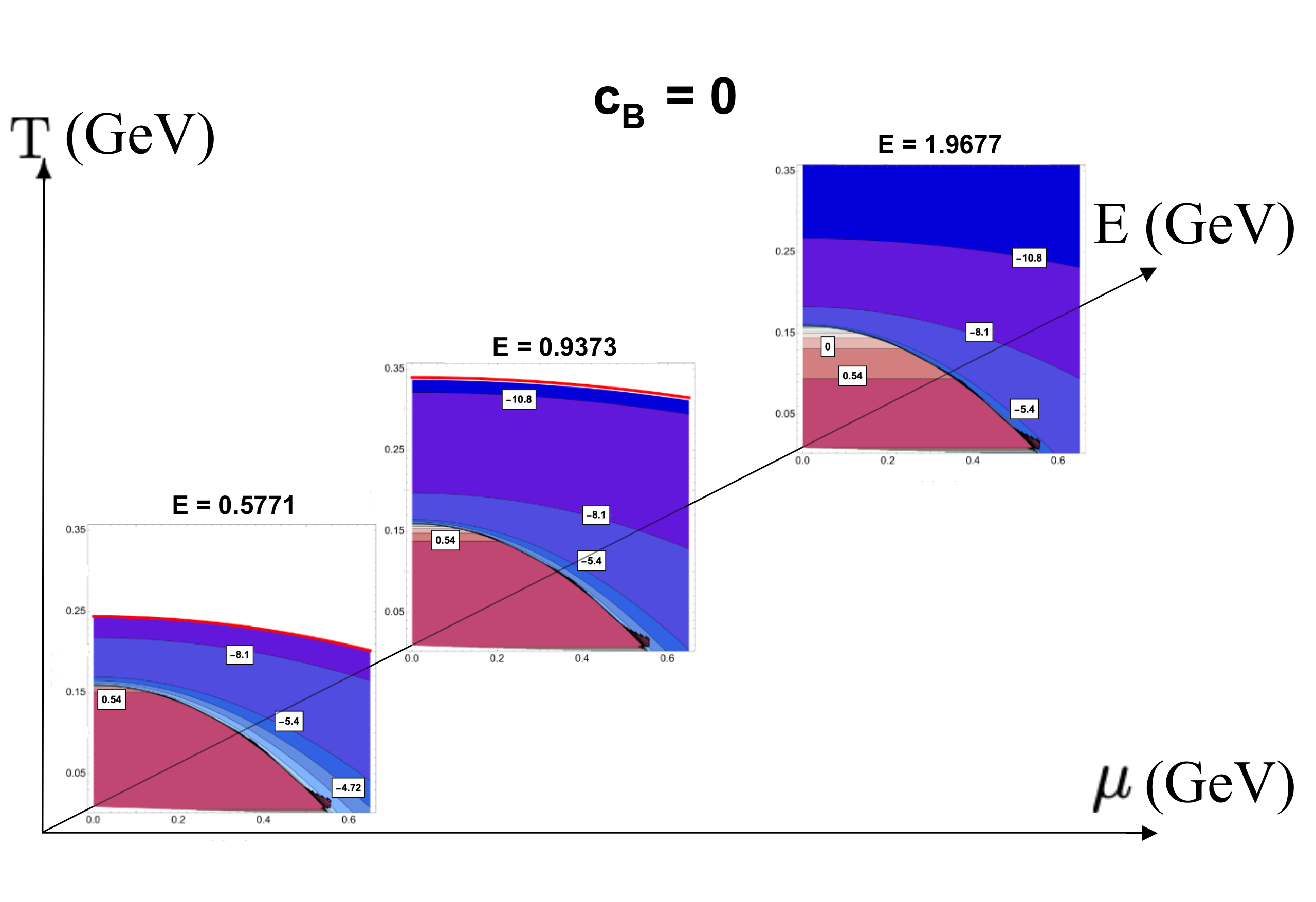
Figure 4: Density plots with contours for $\log\alpha_{\mathfrak{z}}(E;\mu,T)$ at different energy scales $E=\{0.5771,0.9373,1.9677\}$ (GeV) for $c_{B}=0$. The red lines in the first two graphs on the left indicate the maximum possible temperature values at the corresponding energy scale $E$.

In Fig. 5 density plots with contours for $\log\alpha_{\mathfrak{z}}(E;\mu,T)$ at different energy scales $E=\{0.5771,0.9373,1.9677\}$ (GeV) for $c_{B}=-0.05$ ${{GeV}^{2}}$ are arranged in such a way that they represent a family of sections of three-dimensional space $(E,\mu,T)$. In hadronic phase of Fig. 4 in the isotropic case the running coupling constant almost doesn’t depend on the chemical potential. For the anisotropic case Fig. 5 this effect becomes weaker.

Comparing Fig. 4 and Fig. 5 at some fixed parameters $(E,\mu,T)$ shows that increasing magnetic field decreases value of the running coupling constant.

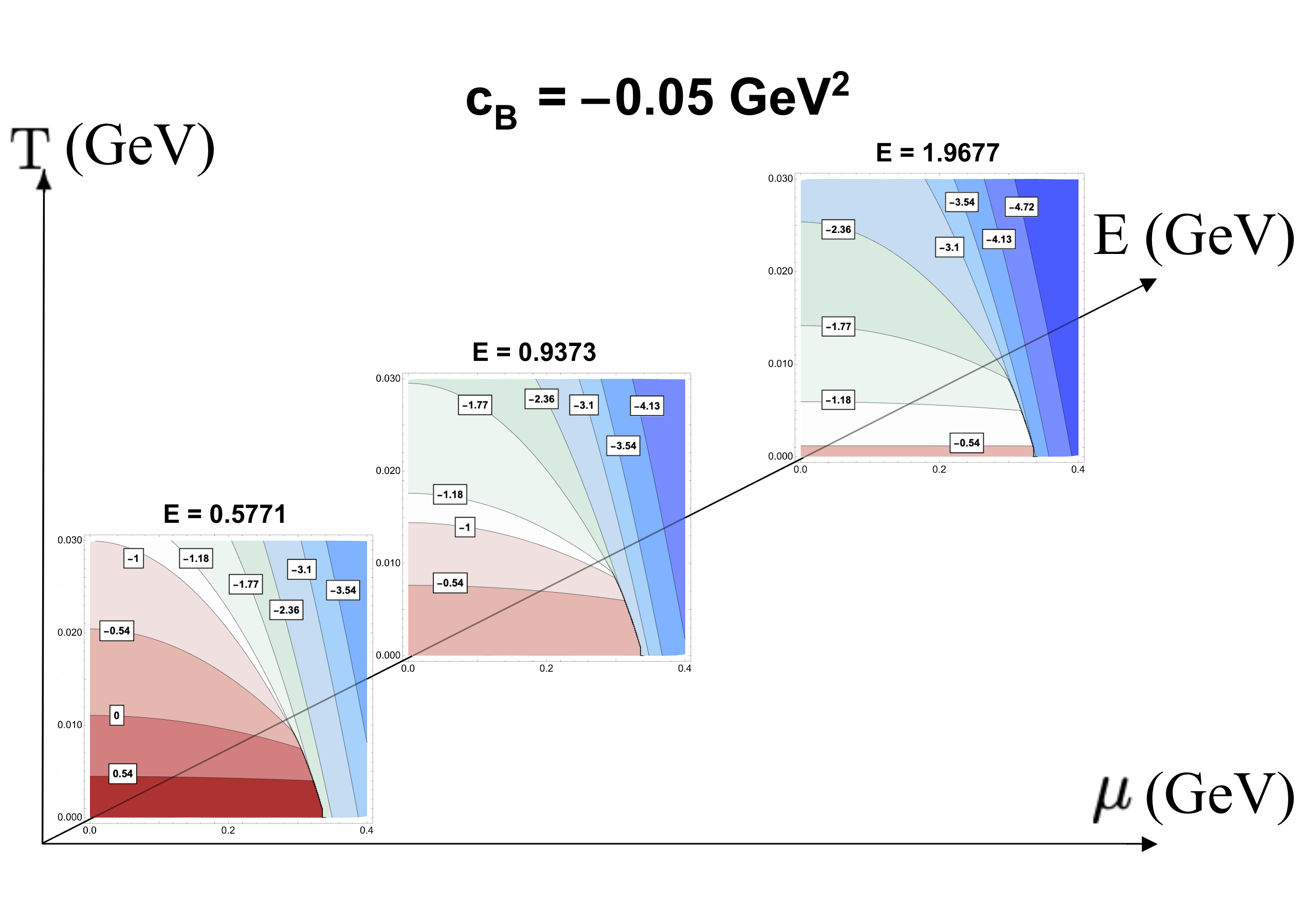
Figure 5: Density plots with contours for $\log\alpha_{\mathfrak{z}}(E;\mu,T)$ at different energy scales $E=\{0.5771,0.9373,1.9677\}$ (GeV) for $c_{B}=-0.05$ GeV².

4 Conclusion

In this paper we have considered an anisotropic holographic model including a strong magnetic field for the light quarks [28]. It is characterized by the Einstein-dilaton-three-Maxwell action and the 5-dimensional metric with the warp factor that has been considered in isotropic case for the light quarks [29]. Our model has two different types of anisotropy, i.e. the spatial anisotropy related to the parameter $\nu$, and the anisotropy related to the external magnetic field described by the third Maxwell field. Particularly, in this paper we considered the second type of anisotropy, i.e. non-zero external magnetic field, and ignored the spatial anisotropy.

It is also very important to note that different boundary conditions lead to different physical consequences. Only (3.6) boundary condition for light quarks leads to physical results in accordance with lattice calculations for non-zero temperature and zero chemical potential [40].

• Magnetic field decreases the value of the running coupling constant $\alpha$ at fixed values of the $T$ and $\mu$.

• The running coupling $\alpha$ decreases with increasing of the energy scale $E$ at the fixed values of $T$ and $\mu$, and such a behavior also persists in the presence of the magnetic field.

• In the region of the hadronic phase, the running coupling $\alpha$ changes slowly with changing in chemical potential, both for an isotropic $c_{B}=0$ and for an anisotropic $c_{B}\neq 0$ cases.

• On the 1-st order transition line, the running coupling has a jump. The magnitude of the jump decreases along the line of the 1-st order transition to get zero in the CEP.

Let us remind that the twice anisotropic model for the light quarks is much more complicated than the twice anisotropic model for heavy quarks [3], since the deformation factor and the kinetic gauge function $f{{}_{1}}$ have more compound form. The effect of magnetic field on the running coupling $\alpha$ in heavy quarks model will be studied in future works.

5 Acknowledgments

We thank K. Runnu and M. Usova for useful discussions. The work of I.A., P.S., A.N is supported by RNF grant 20-12–00200. The work of A.H. was performed at the Steklov International Mathematical Center and supported by the Ministry of Science and Higher Education of the Russian Federation (Agreement No.075-15-2022-265).

 

Appendix

Appendix A Solution to EOMs

To solve EOM (2.5)–(2.11) we need to determine the form of the coupling function $f_{1}$. We take them as in the paper [2]. Taking into account the “light quarks” warp factor, we get

$$f_{1}=e^{-cz^{2}-{\mathcal{A}}(z)}z^{-2+\frac{2}{\nu}}=(1+bz^{2})^{a}\,e^{-cz^{2}}z^{-2+\frac{2}{\nu}}\,,$$ (A.1)

where $c=0.227$ GeV². Solving (2.6) with the coupling function (A.1) and boundary conditions (2.12) gives

$$A_{t}=\mu\,\cfrac{e^{\left(2c-c_{B}\right)z^{2}/2}-e^{\left(2c-c_{B}\right)z_{h}^{2}/2}}{1-e^{\left(2c-c_{B}\right)z_{h}^{2}/2}}\,.$$ (A.2)

We get an expression for the function $f_{B}$

$$f_{B}=2\left(\cfrac{z}{L}\right)^{-2/\nu}\!\!\!\mathfrak{b}g\,\cfrac{c_{B}z}{q_{B}^{2}}\left(\cfrac{3\mathfrak{b}^{\prime}}{2\mathfrak{b}}-\cfrac{2}{\nu z}+c_{B}z+\cfrac{g^{\prime}}{g}\right),$$ (A.3)

and get the solution for blackening function:

$$g=e^{c_{B}z^{2}}\left[1-\cfrac{I_{1}(z)}{I_{1}(z_{h})}+\cfrac{\mu^{2}\,(2c-c_{B})\,I_{2}(z)}{L^{2}\left(1-e^{\left(2c-c_{B}\right)z_{h}^{2}/2}\right)^{2}}\left(1-\cfrac{I_{1}(z)}{I_{1}(z_{h})}\,\cfrac{I_{2}(z_{h})}{I_{2}(z)}\right)\right],$$ (A.4)

where

$$I_{1}(z)=\int_{0}^{z}\left(1+b\xi^{2}\right)^{3a}e^{-3c_{B}\xi^{2}/2}\,\xi^{1+\frac{2}{\nu}}\,d\xi,$$ (A.5)

$$I_{2}(z)=\int_{0}^{z}\left(1+b\xi^{2}\right)^{3a}e^{\left(c-2c_{B}\right)\xi^{2}}\,\xi^{1+\frac{2}{\nu}}\,d\xi.$$ (A.6)

Further solving (2.5)–(2.11) system with the coupling functions (A.1) and (A.3) and the boundary condition (2.14) gives

$$f_{2}=2\left(\cfrac{z}{L}\right)^{2-4/\nu}\,\cfrac{\nu-1}{q^{2}\nu^{2}z^{2}}\,\cfrac{e^{c_{B}z^{2}}}{(1+bz^{2})^{2a}}\left\{\left(2+2\nu-\nu c_{B}z^{2}+\cfrac{6ab\nu z^{2}}{1+bz^{2}}\right)g-g^{\prime}\nu z\right\},$$ (A.7)

$$\varphi=\int_{z_{0}}^{z}\sqrt{\cfrac{4(\nu-1)}{\nu^{2}\xi^{2}}-2c_{B}\left(3-\cfrac{2}{\nu}\right)-2c_{B}^{2}\xi^{2}+\cfrac{12ab}{1+b\xi^{2}}\left(1+2\,\cfrac{1+ab\xi^{2}}{1+b\xi^{2}}\right)}\,d\xi,$$ (A.8)

$$\varphi^{\prime}=\sqrt{\cfrac{4(\nu-1)}{\nu^{2}z^{2}}-2c_{B}\left(3-\cfrac{2}{\nu}\right)-2c_{B}^{2}z^{2}+\cfrac{12ab}{1+bz^{2}}\left(1+2\,\cfrac{1+abz^{2}}{1+bz^{2}}\right)},$$ (A.9)

$$\begin{split}&V(z)=-\,\cfrac{(1+bz^{2})^{2a}\ z}{2L^{2}}\ \times\\ &\left[2\left\{2\,\cfrac{(1+\nu)(1+2\nu)+\bigl{(}2+(2+3a)(3+2\nu)\nu\bigr{)}bz^{2}+(1+\nu+3a\nu)(1+2\nu+6a\nu)b^{2}z^{4}}{(1+bz^{2})^{2}\nu^{2}z^{2}}\right.\right.\\ &\left.-\left.c_{B}\left(2+\cfrac{3}{\nu}+\cfrac{12abz^{2}}{1+bz^{2}}\right)+c_{B}^{2}z^{2}\right\}g\,z-\left(5+3\left(\cfrac{6ab}{1+bz^{2}}-c_{B}\right)z^{2}+\cfrac{4}{\nu}\right)g^{\prime}+g^{\prime\prime}z\right].\end{split}$$ (A.10)

Note, that we do not fix coupling function for the 3-rd Maxwell $f_{B}$, but derive it from the EOM with intent. Fixing, for example, $f_{B}=f_{1}$ makes system (2.5)–(2.11) not selfconsistent, therefore proper solution with the $f_{B}=f_{1}$ condition can’t be found.

References

- [1] I. Y. Aref’eva, A. Hajilou, P. Slepov and M. Usova, “Running Coupling and Beta-Functions for HQCD with Heavy and Light Quarks: Isotropic case,” [arXiv:2402.14512 [hep-th]].
- [2] I. Y. Aref’eva, A. Ermakov, K. Rannu and P. Slepov, “Holographic model for light quarks in anisotropic hot dense QGP with external magnetic field,” Eur. Phys. J. C 83, no.1, 79 (2023) [arXiv:2203.12539 [hep-th]].
- [3] I. Y. Aref’eva, K. Rannu and P. Slepov,“Holographic model for heavy quarks in anisotropic hot dense QGP with external magnetic field,”JHEP 07, 161 (2021) [arXiv:2011.07023 [hep-th]].
- [4] R. L. Workman et al. [Particle Data Group], “Review of Particle Physics,” PTEP 2022, 083C01 (2022).
- [5] I. Y. Aref’eva, ”Remarks on comparison of holographic running coupling with experimental data”, in preparation.
- [6] H. J. Pirner and B. Galow, “Strong Equivalence of the AdS-Metric and the QCD Running Coupling”, Phys. Lett. B 679, 51-55 (2009) [arXiv:0903.2701 [hep-ph]].
- [7] B. Galow, E. Megias, J. Nian and H. J. Pirner, “Phenomenology of AdS/QCD and Its Gravity Dual,” Nucl. Phys. B 834, 330-362 (2010) [arXiv:0911.0627 [hep-ph]].
- [8] S. J. Brodsky, G. F. de Teramond and A. Deur, “Nonperturbative QCD Coupling and its -function from Light-Front Holography,” Phys. Rev. D 81, 096010 (2010) [arXiv:1002.3948 [hep-ph]].
- [9] A. Deur, S. J. Brodsky and C. D. Roberts, “QCD running couplings and effective charges,” Prog. Part. Nucl. Phys. 134, 104081 (2024) [arXiv:2303.00723 [hep-ph]].
- [10] D. S. Gorbunov and V. A.Rubakov. “Introduction to the theory of the early universe: Cosmological perturbations and inflationary theory”. World Scientific, 2011.
- [11] J. M. Lattimer and M. Prakash M. The equation of state of hot, dense matter and neutron stars, Phys. Rep. 621 (2016) 127-164.
- [12] A. Lovato, T. Dore, R. D. Pisarski, B. Schenke, K. Chatziioannou, J. S. Read, P. Landry, P. Danielewicz, D. Lee and S. Pratt, et al. “Long Range Plan: Dense matter theory for heavy-ion collisions and neutron stars,” [arXiv:2211.02224 [nucl-th]].
- [13] L. Du, A. Sorensen and M. Stephanov, “The QCD phase diagram and Beam Energy Scan physics: a theory overview,” [arXiv:2402.10183 [nucl-th]].
- [14] J. M. Maldacena, “The Large N limit of superconformal field theories and supergravity,” Adv. Theor. Math. Phys. 2, 231-252 (1998). [arXiv:hep-th/9711200 [hep-th]].
- [15] J. Casalderrey-Solana, H. Liu, D. Mateos, K. Rajagopal and U. A. Wiedemann, “Gauge/String Duality, Hot QCD and Heavy Ion Collisions”, (Cambridge University Press, Cambridge, UK, 2014), [arXiv:1101.0618 [hep-th]].
- [16] I. Y. Aref’eva, “Holographic approach to quark-gluon plasma in heavy ion collisions”, Phys. Usp. 57, 527-555 (2014).
- [17] O. DeWolfe, S. S. Gubser, C. Rosen and D. Teaney, “Heavy ions and string theory”, Prog. Part. Nucl. Phys. 75, 86 (2014) [arXiv:1304.7794 [hep-th]].
- [18] L. Adamczyk et al. [STAR], “Observation of an Energy-Dependent Difference in Elliptic Flow between Particles and Antiparticles in Relativistic Heavy Ion Collisions,” Phys. Rev. Lett. 110, no.14, 142301 (2013).
- [19] J. Adams et al. [STAR], “Experimental and theoretical challenges in the search for the quark gluon plasma: The STAR Collaboration’s critical assessment of the evidence from RHIC collisions,” Nucl. Phys. A 757, 102-183 (2005).
- [20] B. I. Abelev et al. [STAR], “Identified particle production, azimuthal anisotropy, and interferometry measurements in Au+Au collisions at s(NN)**(1/2) = 9.2- GeV,” Phys. Rev. C 81, 024911 (2010).
- [21] X. Luo and N. Xu, “Search for the QCD Critical Point with Fluctuations of Conserved Quantities in Relativistic Heavy-Ion Collisions at RHIC : An Overview,” Nucl. Sci. Tech. 28, no.8, 112 (2017) [arXiv:1701.02105 [nucl-ex]].
- [22] P. Huovinen and P. V. Ruuskanen, “Hydrodynamic Models for Heavy Ion Collisions,” Ann. Rev. Nucl. Part. Sci. 56, 163-206 (2006).
- [23] U. Gursoy, M. Jarvinen and G. Nijs, “Holographic QCD in the Veneziano Limit at a Finite Magnetic Field and Chemical Potential”, Phys. Rev. Lett. 120, no.24, 242002 (2018) [arXiv:1707.00872 [hep-th]].
- [24] I. Y. Aref’eva, K. A. Rannu and P. S. Slepov, “Dense QCD in Magnetic Field”, Phys. Part. Nucl. Lett. 20 (2023) no.3, 433-437.
- [25] H. Bohra, D. Dudal, A. Hajilou and S. Mahapatra, “Anisotropic string tensions and inversely magnetic catalyzed deconfinement from a dynamical AdS/QCD model,” Phys. Lett. B 801, 135184 (2020) [arXiv:1907.01852 [hep-th]].
- [26] I. Y. Aref’eva, A. Hajilou, K. Rannu and P. Slepov, “Magnetic catalysis in holographic model with two types of anisotropy for heavy quarks,” Eur. Phys. J. C 83, no.12, 1143 (2023) [arXiv:2305.06345 [hep-th]].
- [27] Y. Chen, X. Chen, D. Li and M. Huang, “Deconfinement and chiral restoration phase transition under rotation from holography in an anisotropic gravitational background,” [arXiv:2405.06386 [hep-ph]].
- [28] I. Y. Aref’eva, K. A. Rannu and P. S. Slepov, “Anisotropic solution of the holographic model of light quarks with an external magnetic field,” Theor. Math. Phys. 210, no.3, 363-367 (2022).
- [29] M. W. Li, Y. Yang and P. H. Yuan, “Approaching Confinement Structure for Light Quarks in a Holographic Soft Wall QCD Model,” Phys. Rev. D 96, no.6, 066013 (2017) [arXiv:1703.09184 [hep-th]].
- [30] Y. Yang and P. H. Yuan, “Confinement-deconfinement phase transition for heavy quarks in a soft wall holographic QCD model,” JHEP 12, 161 (2015) [arXiv:1506.05930 [hep-th]].
- [31] I. Y. Aref’eva, K. Rannu and P. Slepov, “Holographic anisotropic model for light quarks with confinement-deconfinement phase transition,” JHEP 06, 090 (2021) [arXiv:2009.05562 [hep-th]].
- [32] I. Y. Aref’eva and A. A. Golubtsova, “Shock waves in Lifshitz-like spacetimes,” JHEP 04, 011 (2015) [arXiv:1410.4595 [hep-th]].
- [33] I. Aref’eva and K. Rannu, “Holographic Anisotropic Background with Confinement-Deconfinement Phase Transition,” JHEP 05, 206 (2018) [arXiv:1802.05652 [hep-th]].
- [34] I. Aref’eva, K. Rannu and P. Slepov, “Orientation Dependence of Confinement-Deconfinement Phase Transition in Anisotropic Media,” Phys. Lett. B 792, 470-475 (2019) [arXiv:1808.05596 [hep-th]].
- [35] H. Bohra, D. Dudal, A. Hajilou and S. Mahapatra, “Chiral transition in the probe approximation from an Einstein-Maxwell-dilaton gravity model,” Phys. Rev. D 103, no.8, 086021 (2021) [arXiv:2010.04578 [hep-th]].
- [36] E. D’Hoker and P. Kraus, “Charged Magnetic Brane Solutions in AdS (5) and the fate of the third law of thermodynamics,” JHEP 03, 095 (2010) [arXiv:0911.4518 [hep-th]].
- [37] U. Gursoy and E. Kiritsis, “Exploring improved holographic theories for QCD: Part I,” JHEP 02, 032 (2008) [arXiv:0707.1324 [hep-th]].
- [38] U. Gursoy, E. Kiritsis and F. Nitti, “Exploring improved holographic theories for QCD: Part II”, JHEP 02, 019 (2008) [arXiv:0707.1349 [hep-th]].
- [39] N. Cardoso and P. Bicudo, “Lattice QCD computation of the SU(3) String Tension critical curve,” Phys. Rev. D 85, 077501 (2012) [arXiv:1111.1317 [hep-lat]].
-
[40]
O. Kaczmarek,
“Screening at finite temperature and density,”
PoS CPOD07, 043 (2007)
[arXiv:0710.0498 [hep-lat]].