Revisiting primordial magnetic fields through 21-cm physics: Bounds and forecasts

Abstract

Primordial magnetic fields (PMFs) may significantly influence 21-cm physics via two mechanisms: (i) magnetic heating of the intergalactic medium (IGM) through ambipolar diffusion (AD) and decaying magnetohydrodynamic turbulence (DT), (ii) impact on the star formation rate density (SFRD) through small-scale enhancement of the matter power spectrum. In this analysis, we integrate both of these effects within a unified analytical framework and use it to determine upper bounds on the parameter space of a nearly scale-invariant non-helical PMF in the light of the global 21-cm signal observed by EDGES. Our findings reveal that the joint consideration of both effects furnishes constraints of the order $B_{0}\lesssim\mathcal{O}(10^{-2})$ nG on the present-day magnetic field strength, which are considerably tighter compared to earlier analyses. We subsequently explore the prospects of detecting such a magnetized 21-cm power spectrum at the upcoming SKA-Low mission. For the relevant parameters of the PMF ($B_{0}$ and $n_{\!{}_{B}}$) and the excess radio background ($\xi$), SNR estimation and Fisher forecast analysis indicate that it may be possible to constrain these three parameters with relative $1\sigma$ uncertainties $\lesssim 10\%$ and an associated SNR $\gtrsim 10$ at SKA-Low. This also leads to possible correlations among these three parameters, thus revealing intriguing trends of interplay among the various physical processes involved.

1 Introduction

The presence of very weak magnetic fields on cosmic scales has been hinted at for decades by several independent observations. In particular, it is currently known that magnetic fields typically of strength $10^{-15}\>\textrm{G}<B_{0}<10^{-9}\>\textrm{G}$ at the present day may permeate the voids of the intergalactic medium (IGM) across length scales of $\mathcal{O}(1)\>\rm{Mpc}$, where the $\mathcal{O}(\rm{nG})$ upper bound is furnished by Faraday rotation measures of extragalactic sources [1, 2, 3, 4] and cosmic microwave background (CMB) constraints [5, 6, 7], while the lower bound results from the null detection of secondary (GeV) $\gamma$-ray cascades triggered in the IGM by primary (TeV) $\gamma$-emissions from distant blazars [8, 9, 10]. The inadequacy of bottom-up astrophysical dynamo mechanisms [11, 12, 13, 14] when it comes to the explanation of such large-scale volume-filling magnetic fields indicates a possible primordial origin of these fields, which may be produced, for example, via a wide range of inflationary dynamics [15, 16, 17, 18, 19, 20, 21, 22, 23, 24, 25] or due to phase transitions in the early Universe [26, 27, 28, 29, 30, 31, 32, 33, 34, 35] (for brief reviews on both, see Refs. [36, 37]). Owing to its stochastic nature, such a primordial magnetic field (PMF) is typically characterized by its power spectrum, whose amplitude is governed by the magnetic energy density smoothed on a given scale at present time ($A_{B}$), and the scale-dependence is regulated by the magnetic spectral index ($n_{\!{}_{B}}$). Constraints on $A_{B}$ can be directly translated to bounds on the present magnetic field strength if its redshift-evolution is properly incorporated, whereas currently available datasets do not put precise constraints on $n_{\!{}_{B}}$, which is usually chosen to be a free parameter while modelling various cosmological effects of PMFs across the various cosmic epochs.

Such ambient magnetic fields are naturally expected to leave some imprints on the redshifted neutral hydrogen (HI) 21-cm signal. Being a treasure trove of information as far as the physics of the dark ages and the cosmic dawn is concerned, the 21-cm observational window could be a potentially important tool in constraining the parameters of the PMF power spectrum as well. A stochastic PMF could be either helical or non-helical in nature. The latter being the minimal scenario from a primordial magnetogenetic point of view [36, 37], we stick to the non-helical PMF only in this work. The key processes through which such a non-helical PMF could affect the 21-cm signal may be classified broadly under two categories, namely IGM heating effects [38, 39, 40, 41, 42] and possible impact on the formation of large scale structure (LSS) [43, 44, 45, 46], both of which are well-studied from theoretical perspectives. The former results from the dissipation of magnetic energy through ambipolar diffusion (AD) and decaying magnetohydrodynamic turbulence (DT) which may heat up the kinetic sector of the gaseous IGM, while the latter can be traced to the small-scale enhancement of matter power induced by a stochastic PMF. The Experiment to Detect the Global EoR Signature (EDGES) [47] has reported an intense depth in the global 21-cm absorption signal $\overline{T}_{21}(z)$ which is in 3.8$\sigma$ tension with the prediction of the vanilla $\Lambda$CDM scenario [48]. Following this detection, the impact of magnetic IGM heating (via AD & DT) on the 21-cm dip was considered in Ref. [49], where an upper limit of $B_{0}\lesssim\mathcal{O}(0.1)$ nG was obtained based on the requirement that the 21-cm signal be in absorption (as observed by EDGES) rather than in emission in an otherwise $\Lambda$CDM background. Magnetic effects on the IGM temperature and resulting PMF constraints in the light of the EDGES detection have subsequently been investigated for various other non-minimal physical scenarios as well, e.g. baryon-dark matter (DM) interactions [50, 51], helical PMF spectra [52], and the presence of excess radio background [53]. One may readily observe that each of these scenarios accommodates some specific mechanism via which the IGM can be sufficiently cooled so as to allow $\overline{T}_{21}(z)=-500^{+200}_{-500}$ mK in the redshift range $16\lesssim z\lesssim 19$ as observed by EDGES.

However, another crucial feature which needs to be taken into account while constraining a PMF on the basis of the existing global 21-cm data is its role in the formation of structure, which is expected to play a significant role in the redshift evolution of $\overline{T}_{21}(z)$ by directly influencing the star formation history of our Universe. While such effects are well explored in the literature via both analytical and simulation-based approaches [54, 55, 56, 57, 58, 59, 60], a detailed investigation of their role in the context of the EDGES signal is lacking in the aforementioned studies, which have focused mostly on the magnetic heating effects in the IGM. The latter results primarily in a vertical shift of the amplitude of $\overline{T}_{21}(z)$, which has been the cornerstone of EDGES-based analysis of PMFs so far. However, modification of the star formation rate density (SFRD) in presence of PMFs should have a significant impact on X-ray heating of the IGM, which is instrumental in determining the redshift of the 21-cm absorption minimum. More precisely, besides the aforementioned vertical change in its depth, one should also expect a lateral shift of the absorption trough towards higher (lower) redshifts if the SFRD is enhanced (suppressed) at earlier times in the presence of PMFs, which therefore provides an additional degree of freedom that may be used to constrain the PMF parameter space on the basis of existing data.

In the present work, we first attempt to bridge this gap by integrating both magnetic heating effects (AD & DT) and the impact of PMFs on the star formation history within a common analytical framework, and use it to derive PMF constraints based on the EDGES window. Because we focus on non-helical PMFs, we necessarily assume an excess radio background in order to achieve the required level of IGM cooling so as to be compatible with the EDGES bounds, as supported by the Absolute Radiometer for Cosmology, Astrophysics, and Diffuse Emission (ARCADE-2) [61] and the Long Wavelength Array (LWA1) [62] experiments. If only magnetic heating effects are considered, the admissible upper bound on $B_{0}$ from EDGES for a nearly scale-invariant PMF can be significantly large and exceed $\mathcal{O}(1)$ nG [53], as magnetic heating can be readily compensated by the large parameter space of the excess radio background, all the while keeping the absorption trough comfortably within $16<z<19$. A magnetically modified SFRD model, however, changes the scenario by directly affecting the redshift at which the trough occurs, and as we find, allows deriving considerably tighter PMF constraints even in the presence of an excess radio background. Our analysis reveals that even for nearly scale-invariant non-helical PMFs, a stringent upper bound of $B_{0}\lesssim\mathcal{O}(10)$ pG may be achieved based primarily on this lateral shift, which appears to be significantly more sensitive to the PMF parameters than the dependence of the vertical depth of the signal on the PMF and the excess radio background combined. Furthermore, our analysis explicitly highlights the deviation from the simple $(1+z)^{2}$ redshift-scaling of the PMF amplitude owing to the dissipation of magnetic energy through AD and DT, which has also been pointed out earlier in [51]. For the typical weak magnetic field strengths involved in this work, this relative deviation turns out to be significant and can lead to $\mathcal{O}(1)$ relative errors in the estimate of $B_{0}$. This has motivated us to model the scenario as a typical initial value problem where the magnetic field at recombination ($B_{\rm CMB}$) serves as the fundamental parameter, while the present day magnetic strength $B_{0}$ is a derived parameter which is subsequently obtained through a full numerical solution instead of being connected to $B_{\rm CMB}$ via an a priori $B_{\rm CMB}=B_{0}(1+z)^{2}$ scaling. Thus, certain results in this work are presented in terms of $B_{\rm CMB}$ wherever deemed suitable.

In the second half of our work, we focus on the joint PMF and excess radio background parameter space that we find to be compatible with the global signal from EDGES, and explore the prospects of further constraints on the same based on 21-cm power spectrum data in the light of the upcoming Square Kilometre Array (SKA) [63, 64, 65, 66, 67]. In terms of HI 21-cm physics, the SKA is expected to be a transformative scientific facility of the ongoing century that would be able to shed light on hitherto unexplored epochs of our cosmic history, ranging from the dark ages at $30\lesssim z\lesssim 100$ all the way up to the epoch of reionization (EoR) around $z\sim 4-12$. The scope of constraining cosmic magnetism on various scales with the SKA have been shown to be promising in numerous earlier works [68, 69, 70, 45, 71]. Thus, in addition to the presently available 21-cm window, it is imperative to assess the prospects of constraining the parameters of the scenario under consideration with future data from the SKA. For this purpose, we first calculate the signal-to-noise ratio (SNR) of the one-dimensional 21-cm power spectrum achievable by the SKA Low Frequency Array (SKA-Low) as a function of the two non-helical PMF parameters ($B_{0}$ and $n_{\!{}_{B}}$) and the ARCADE-2 modelling parameter ($\xi$) [72]. This is followed by a Fisher forecast analysis involving these three parameters, which allows us to estimate their projected $1\sigma$ errors at SKA-Low. For particular fiducial values as allowed by the available parameter space from EDGES, our analysis reveals interesting trends for both the $1\sigma$ error forecasts and possible correlations from SKA-Low, which can be traced back to the interplay among the various physical effects induced by the PMF and the excess radio background.

The work is organised as follows. In Sec. 2, a brief outline of the theoretical framework for modelling the global $\overline{T}_{21}(z)$ signal in the presence of a non-helical PMF has been presented, by taking both IGM heating effects and the possible impact on star formation history into account. In Sec. 3, we present our numerically obtained results for $\overline{T}_{21}(z)$ by including an excess radio background vis-à-vis the observation by EDGES, thereby arriving at sets of upper bounds on $B_{0}$ and $\xi$ for two benchmark values of $n_{\!{}_{B}}=-2.75$ and $n_{\!{}_{B}}=-2.95$ (both representing nearly scale-invariant PMF power spectra). In Sec. 4, we compute the 21-cm power spectra semi-analytically for suitable choices of the parameters that we find to be compatible with EDGES, and proceed to the subsequent estimation of the SNR and the Fisher forecast analysis in the light of SKA-Low in Sec. 5. Finally, Sec. 6 summarizes the key findings and presents a brief discussion on a few important future directions to explore.

2 The global 21-cm signal

2.1 21-cm signal in absence of magnetic field

The principal physical observable under investigation in any 21-cm experiment is the differential brightness temperature, denoted by $T_{21}$. The sky-averaged (global) differential brightness temperature can be expressed as  [73, 74]

$$\overline{T}_{21}(z)\simeq 27x_{\rm HI}\left(\frac{\Omega_{b,0}h^{2}}{0.023}\right)\sqrt{\frac{0.15}{\Omega_{m,0}h^{2}}\frac{1+z}{10}}\left(1-\frac{T_{\gamma}}{T_{s}}\right)\,\,\rm{mK}.$$ (2.1)

where $x_{\rm HI}$ is the neutral hydrogen fraction, and $\Omega_{m,0}$ ($\Omega_{b,0}$) represents the total (baryonic) matter abundance in the Universe at the present epoch. The spin temperature $T_{s}$ can be expressed as a weighted average of the background radiation temperature $T_{\gamma}$, the gas kinetic temperature $T_{k}$, and the Lyman-$\alpha$ temperature $T_{\alpha}$ as [75]

$$T_{s}^{-1}=\frac{T_{\gamma}^{-1}+x_{k}T_{k}^{-1}+x_{\alpha}T_{\alpha}^{-1}}{1+x_{k}+x_{\alpha}}\>,$$ (2.2)

with $x_{k}$ and $x_{\alpha}$ representing the collisional coupling coefficient and the Lyman-$\alpha$ coupling coefficient respectively. In our analysis, we consider $T_{\alpha}\approx T_{k}$, since frequent scattering among the Ly-$\alpha$ photons thermally equilibrate $T_{\alpha}$ and $T_{k}$ [74, 76]. The coefficient $x_{k}$, incorporating three interaction channels (H-H, H-e, and H-p collisions), depends strongly on $T_{k}$  [77, 78]. On the other hand, $x_{\alpha}$ encapsulates the Lyman-$\alpha$ flux ($J_{\alpha}$) [78, 79] and depends on the SFRD, which can be expressed as [80, 81, 82]

$$\dot{\rho}_{\star}(z)=-f_{\star}\Omega_{b,0}\rho_{c,0}(1+z)H(z)\dfrac{d}{dz}f_{\rm coll}(z)\>,$$ (2.3)

where $\rho_{c,0}\equiv\frac{3H_{0}^{2}}{8\pi G}$ is the critical density of the Universe at the present epoch and $f_{\star}$ represents the stellar-to-baryon ratio. Throughout this work, we have used $f_{\star}=0.01$ which aligns well with findings from radiation-hydrodynamic simulations of high-redshift galaxies [83, 84]. In the Press-Schechter (PS) formalism of spherical halo collapse [85], the collapse function can be expressed as $f_{\rm coll}(z)=\textrm{erfc}\left(\frac{1.686(1+z)}{\sqrt{2}\sigma(R(z))}\right)$, where $\sigma^{2}$ is the mean-squared mass variance smoothed over a window function $W(k,R)$ of characteristic length scale $R(z)$ as

$$\sigma^{2}(R(z))=\dfrac{1}{2\pi^{2}}\int\limits_{0}^{\infty}k^{2}P_{m}^{(\rm tot)}(k)|W(k,R(z))|^{2}\>.$$ (2.4)

Here, $P_{m}^{(\rm tot)}$ denotes the total matter power spectrum of the Universe at the present epoch.

In order to model the global 21-cm signal, we additionally need the ionization histories of HI and HeI, whose ionizations fractions evolve as  [86]

$${dx_{\rm p}\over dz} =\left(x_{\rm e}x_{\rm p}n_{\rm\!{}_{H}}\alpha_{\rm\!{}_{H}}-\beta_{\rm\!{}_{H}}(1-x_{\rm p}){\rm e}^{-h_{\!{}_{P}}\nu_{\!{}_{H2s}}/k_{\!{}_{B}}T_{k}}\right)$$

$$\times\quad{\left(1+K_{\rm\!{}_{H}}\Lambda_{\rm\!{}_{H}}n_{\rm\!{}_{H}}(1-x_{\rm p})\right)\over H(z)(1+z)\left(1+K_{\rm\!{}_{H}}(\Lambda_{\rm\!{}_{H}}+\beta_{\rm\!{}_{H}})n_{\rm\!{}_{H}}(1-x_{\rm p})\right)},$$

$${dx_{\rm\!{}_{He}}\over dz}= \left(x_{\rm\!{}_{He}}x_{\rm e}n_{\rm\!{}_{H}}\alpha_{\rm\!{}_{He}}-\beta_{\rm\!{}_{He}}(f_{\rm\!{}_{He}}-x_{\rm\!{}_{He}}){\rm e}^{-h_{\!{}_{P}}\nu_{\!{}_{He2^{1}s}}/k_{\!{}_{B}}T_{k}}\right)$$

$$\times{\left(1+K_{\rm\!{}_{He}}\Lambda_{\rm\!{}_{He}}n_{\rm\!{}_{H}}(f_{\rm\!{}_{He}}-x_{\rm\!{}_{He}}){\rm e}^{-h_{\!{}_{P}}\nu_{\!{}_{ps}}/k_{\!{}_{B}}T_{k}})\right)\over H(z)(1+z)\left(1+K_{\rm\!{}_{He}}(\Lambda_{\rm\!{}_{He}}+\beta_{\rm\!{}_{He}})n_{\rm\!{}_{H}}(f_{\rm\!{}_{He}}-x_{\rm\!{}_{He}}){\rm e}^{-h_{\!{}_{P}}\nu_{\!{}_{ps}}/k_{\!{}_{B}}T_{k}}\right)}.$$

The total electron fraction ($x_{\rm e}$) is subsequently defined to be

$$x_{\rm e}=x_{\rm p}+x_{\rm\!{}_{He}},$$ (2.7)

where $x_{\rm p}\equiv\frac{n_{\rm p}}{n_{\!{}_{\rm H}}}$ and $x_{\rm\!{}_{He}}\equiv\frac{n_{\rm\!{}_{He}}}{n_{\!{}_{\rm H}}}$ are the proton fraction and singly ionized helium fraction, respectively, with $n$ referring the number density (see appendix A for further details.). Finally, the evolution of the gas kinetic temperature ($T_{k}$) of the IGM is expressed as [78]

$$\frac{dT_{k}}{dz}=\frac{2T_{k}}{1+z}-\frac{2}{3H(z)(1+z)}\sum_{i}\frac{\epsilon_{i}}{k_{\!{}_{B}}n_{\rm tot}},$$ (2.8)

where the first term represents adiabatic cooling due to cosmic expansion, and each subsequent $\epsilon_{i}$ term accounts for the energy injection/extraction rate per unit volume corresponding to the $i$^th process. In the baseline $\Lambda$CDM scenario, two effects may reflect on the IGM temperature on top of adiabatic cooling:

1. Compton scattering between electrons and photons: The rate of energy transfer per unit volume due to Compton effect can be expressed as [87]

   $$\epsilon_{\rm comp}=\frac{3}{2}nk_{\!{}_{B}}\frac{x_{\rm e}}{1+x_{\rm e}+f_{\!{}_{\rm He}}}\frac{8\sigma_{\!{}_{T}}u_{\gamma}}{3m_{e}c}\left(T_{\gamma}-T_{k}\right)\>,$$ (2.9)

   with $\sigma_{\!{}_{T}}$ and $u_{\gamma}$ respectively denoting the Thomson cross-section and the energy density of background photons.

2. X-ray heating: The X-ray photons produced from galaxies and clusters after star formation can heat the IGM at comparatively lower redshifts, for which the energy injection rate per unit volume is modelled as  [78]

   $$\epsilon_{X}=3.4\times 10^{33}f_{\rm heat}f_{\!{}_{\rm X}}\frac{\dot{\rho}_{\star}(z)}{M_{\rm sun}\,\rm yr^{-1}\,\rm Mpc^{-3}}\,\rm J\,\rm s^{-1}\,\rm Mpc^{-3}\>,$$ (2.10)

   with $M_{\rm sun}$ being the mass of the Sun. Additionally, $f_{\rm heat}$ and $f_{\!{}_{\rm X}}$ are respectively the X-ray heating fraction and the normalization factor accounting for the difference between local and high redshift observations, both of which we fix at $0.2$ based on Refs. [88, 89, 78].

Upon the inclusion of PMFs however, there can be non-trivial impact on the matter clustering and the gas kinetic temperature. These non-trivial impacts strongly affect the star formation rate, ionization history and the global 21-cm signal, whose modelling is discussed in the following section.

2.2 Signatures of PMF on the global 21-cm signal

The effects of a non-helical stochastic PMF on the global 21-cm signal is expected to arise through two simultaneous pathways. Firstly, the PMF is capable of directly heating the IGM by transferring energy from the magnetic sector to the kinetic sector through the processes of ambipolar diffusion (AD) and decaying magnetohydrodynamic turbulence (DT). Secondly, the PMF can significantly enhance matter clustering at small scales ($k/h\gtrsim 1$ Mpc^-1) by sourcing density perturbations via Lorentz force, thereby resulting in a robust signature on SFRD, which, in turn, strongly affects the $x_{\alpha}$. In what follows, we briefly discuss these two phenomena.

2.2.1 Impact of PMF on IGM temperature

AD and DT inject energy into the IGM, resulting in an increment of the gas temperature $T_{k}$. The energy injection rate per unit volume due to these two effects can be expressed as [51]

$$\epsilon_{\rm ambi}(z) \approx \frac{(1-x_{\rm e})}{\gamma\,x_{\rm e}\,(M_{\!{}_{\rm H}}n_{\!{}_{b}})^{2}}\ \frac{E_{B}^{2}\,f_{\!{}_{L}}(n_{\!{}_{B}}+3)}{L_{d}^{2}}\,,$$ (2.11)

$$\epsilon_{\rm turb}(z) = \frac{1.5\ m\ \left[\ln(1+t_{i}/t_{d})\right]^{m}}{\left[\ln(1+t_{i}/t_{d})+1.5\ln\{(1+z_{i})/(1+z)\}\right]^{m+1}}H(z)\,E_{B}\,.$$ (2.12)

Here, $\gamma\approx 1.94\times 10^{11}(T_{k}/K)^{0.375}$ m³kg^-1s^-1 is the coupling coefficient between ionized and neutral baryon components, $E_{B}=|B|^{2}/8\pi$ is the energy density of the magnetic field (written in Gaussian units), $f_{\!{}_{L}}(x)\equiv 0.8313\left(1-1.02\times 10^{-2}x\right)x^{1.105}$, $m\equiv 2(n_{\!{}_{B}}+3)/(n_{\!{}_{B}}+5)$, $t_{i}$ and $t_{d}$ are respectively the physical time scales at which magnetic turbulence becomes dominant and over which it decays and are interrelated as $t_{i}/t_{d}\approx 14.8(B_{0}/\textrm{nG})^{-1}(k_{D}/\textrm{Mpc}^{-1})^{-1}$, and $L_{d}$ is the magnetic damping length scale defined as $L_{d}^{-1}=(1+z)k_{D}$ [51]. The smallest relevant value of the damping wavenumber $k_{D}$ used in these expressions depends on the photon diffusion scale at decoupling, and can be estimated from [90] for best fit values of the background cosmological parameters as

$$k_{D}(z)\>\approx\>\alpha(z)k_{\gamma}\quad;\quad\alpha=\left(\dfrac{B(z)}{\sqrt{16\pi\rho_{\gamma}(z)/3}}\right)^{-1}\>,$$ (2.13)

where $k_{\gamma}$ represents the photon diffusion scale at decoupling. Thus, the magnetic damping wavenumber at decoupling is a function of the magnetic field strength at decoupling ($B_{\rm CMB}$) and the photon energy density at decoupling ($\rho_{\gamma,\textrm{CMB}}$). If one neglects IGM heating effects or assumes them to be negligibly small compared to Hubble expansion, then the frozen-in magnetic field redshifts as $a^{-2}$ and the photon energy density as $a^{-4}$, which removes any redshift dependence from Eq. (2.13) and allows one to use their present values instead, i.e. $B_{0}$ and $\rho_{\gamma,0}$. This is, in fact, what has been done in the majority of studies carried out in the past. However, at lower redshifts, IGM heating via ambipolar diffusion and decaying turbulence are not necessarily sub-dominant effects compared to Hubble evolution of the magnetic field, and the relative error in estimating the present day $B_{0}$ from $B_{\textrm{CMB}}$ through the simple relation $B_{\textrm{CMB}}=B_{0}(1+z_{\rm CMB})^{2}$ increases for smaller values of the magnetic field strength. Thus, in our analysis, we use $B_{\rm CMB}$ directly as the input parameter in Eq. (2.13) to estimate $k_{D}$, which obviates the need to assume any redshift dependence of $B(z)$ a priori. For the photon energy density, of course, one needs to use $\rho_{\gamma,\textrm{CMB}}=\rho_{\gamma,0}(1+z_{\rm CMB})^{4}$.

Furthermore, Eq. (2.12) contains the ratio $t_{i}/t_{d}$, which is estimated conventionally in the literature as a function of $B_{0}$ [49, 51]. This might seem problematic for an initial value problem such as ours, where we can only obtain $B_{0}$ by supplying an initial $B_{\rm CMB}$ as input and solving the coupled first order system. Upon closer inspection though, it becomes clear that the dependence of $\epsilon_{\rm turb}(z)$ on $t_{i}/t_{d}$ is firstly logarithmic, and secondly further suppressed by an overall factor of $m$ which is much smaller than unity if $n_{\!{}_{B}}\to-3$, i.e. the magnetic spectrum is nearly scale-invariant. These two observations allow us to approximate the value of $B_{0}$ appearing in $t_{i}/t_{d}$ as $B_{0}\approx B_{\rm CMB}(1+z_{\rm CMB})^{-2}$. Although this relation is not strictly accurate in presence of heating effects as already explained, the error incurred by this approximation in the specific case of Eq. (2.12) is negligible in view of the aforementioned factors. Throughout our analysis, we also restrict our attention to a nearly scale-invariant PMF, which further justifies this approximation in Eq. (2.12). We reiterate that this is not to be identified/confused with the true value of the present day magnetic field strength, which can only be obtained by solving the full system with appropriate initial conditions. That being said, however little the error might be in the present scenario, we intend to revisit this issue in future and explore some better theoretical modelling of the DT effect within the initial value framework.

Finally, taking both Eqs. (2.11) and (2.12) into account, the evolution of the magnetic field strength itself is governed by the equation

$$\frac{dE_{B}}{dz}=4\,\left(\frac{E_{B}}{1+z}\right)+\frac{1}{(1+z)\,H(z)}\, \left[\epsilon_{\rm ambi}(z)+\,\epsilon_{\rm turb}(z)\,\right]\>,$$ (2.14)

which succinctly captures the rate of energy transfer from the magnetic sector to the IGM.

2.2.2 Impact of PMF on star formation

The presence of primordial magnetic fields modifies the matter power spectrum on small scales ($k/h\gtrsim 1$ Mpc^-1) through the appearance of an effective Lorentz force source term in the evolution equation of matter density perturbations [91, 92, 93, 94, 95]. The modification shows up primarily as a bump on top of the usual adiabatic matter power spectrum, with its position and height governed by two parameters: the present-day magnetic field strength ($B_{0}$) and the magnetic spectral index ($n_{\!{}_{B}}$). Up to the linear order in perturbation theory, the dominant correction term on top of the adiabatic matter power spectrum $P_{m}^{(ad)}(k)$ at present time is given by [96]

$$P_{m}^{(B)}(k)=\dfrac{2\pi^{2}}{k^{3}}\left(\dfrac{k}{a_{0}H_{0}}\right)^{4}\dfrac{4}{225}(1+z_{eq})^{2}\left(\dfrac{\Omega_{\gamma,0}}{\Omega_{m,0}}\right)^{2}\mathcal{P}_{L^{(0)}}(k)\>,$$ (2.15)

where $\Omega_{\gamma,0}$ is the present-day photon energy fraction and $z_{eq}$ is the redshift of matter-radiation equality. The dimensionless power spectrum $\mathcal{P}_{L^{(0)}}(k)$ arises due to the Lorentz source term, and can be expressed analytically as

$$\mathcal{P}_{L^{(0)}}(k) =\dfrac{9}{\left[\Gamma\left(\frac{n_{\!{}_{B}}+3}{2}\right)\right]^{2}}\left(\dfrac{\rho_{B,0}}{\rho_{\gamma,0}}\right)^{2}\left(\dfrac{k}{k_{D}}\right)^{2(n_{\!{}_{B}}+3)}e^{-\left(\frac{k}{k_{D}}\right)^{2}}$$ (2.16)

$$\times\int\limits_{0}^{\infty}dhh^{n_{\!{}_{B}}+2}e^{-2\left(\frac{k}{k_{D}}\right)^{2}h^{2}}\int\limits_{-1}^{+1}dxe^{2\left(\frac{k}{k_{D}}\right)^{2}hx}(1-2hx+h^{2})^{\frac{n_{\!{}_{B}}-2}{2}}$$

$$\times\left[1+2h^{2}+(1-4h^{2})x^{2}-4hx^{3}+4h^{2}x^{4}\right]\>,$$

where $(\rho_{B,0}/\rho_{\gamma,0})\approx 9.545\times 10^{-8}(B_{0}/\textrm{nG})^{2}$ is the ratio of the present-day magnetic energy density and the photon energy density. While computing the magnetic correction, we make use of the magnetic Jeans cut-off scale given by [97, 90]

$$k_{J}=\left[14.8\left(\dfrac{\Omega_{m}}{0.3}\right)^{0.5}\left(\dfrac{h}{0.7}\right)\left(\dfrac{B_{0}}{1\>\textrm{nG}}\right)^{-1}\right]^{\frac{2}{n_{\!{}_{B}}+5}}\>\textrm{Mpc}^{-1}\>,$$ (2.17)

which appears as a hard cut-off to the magnetically induced matter power spectrum in our calculations. The total matter power spectrum, $P_{m}^{(\rm tot)}(k)$, is then given by $P_{m}^{(\rm tot)}(k)=P_{m}^{(\rm ad)}(k)+P_{m}^{(B)}(k)$. In the linear approximation, the matter power spectrum at any earlier epoch with $z>0$ is given by $P_{m}^{(\rm tot)}(k;z)=D(z)^{2}P_{m}^{(\rm tot)}(k)$, where $D(z)=(1+z)^{-1}$ is the normal growth factor. Based on the total matter power spectrum, the SFRD $\dot{\rho}_{\star}(z)$ can then be calculated according to Eq. (2.3). The magnetically modified redshift-dependence of the SFRD has been shown for a few benchmark values of the PMF parameters in Fig. 1.

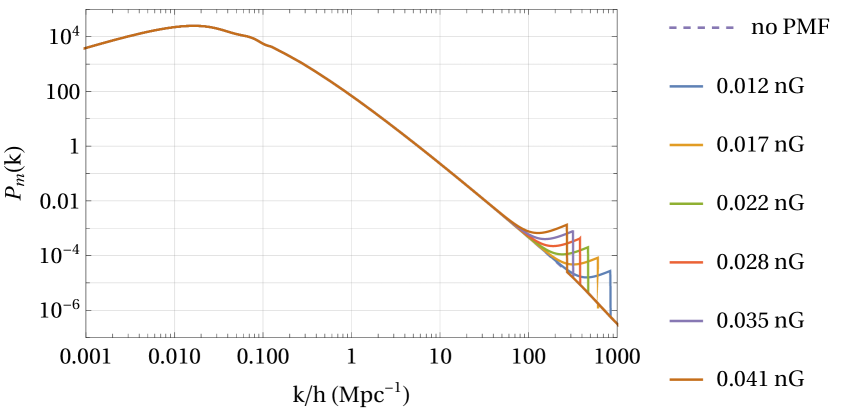
(a)

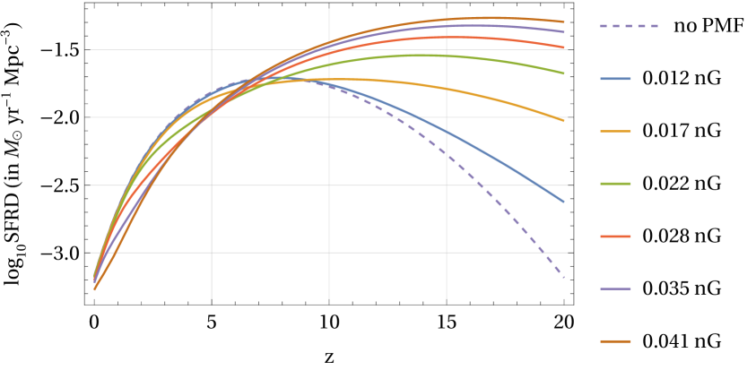
(b)

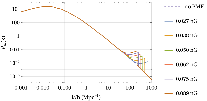
(c)

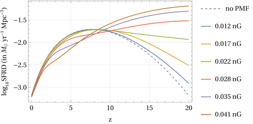
(d)

Figure 1: Impact of primordial magnetic fields on the matter power spectrum and star formation rate density shown for a few representative values of the present day magnetic field strength, with $n_{\!{}_{B}}=-2.75$ (upper panel) and $n_{\!{}_{B}}=-2.95$ (lower panel). Both sets of $B_{0}$ correspond to the same set of $B_{\rm CMB}$ ranging from $7.5\times 10^{4}$ nG to $2.0\times 10^{5}$ nG (in steps of $1.5\times 10^{4}$ nG), thus also reflecting the impact of $n_{\!{}_{B}}$ on the redshift evolution of $B(z)$ through IGM heating effects.

3 Bounds on PMFs from EDGES data

Accounting for both IGM heating effects (AD and DT) and the modified star formation history in presence of non-helical PMFs, we now proceed to estimate the admissible bounds on the PMF parameters based on the global 21-cm signal observed by the EDGES collaboration [47]. The system of first order differential equations to be solved with appropriate initial conditions (defined at decoupling) comprises of Eqs. (2.1), (2.1), (2.8), and (2.14).

As already mentioned, most of the recent analytical studies conducted in this direction either focus solely on IGM heating and do not account for the effect of the PMF on the SFRD [49, 50, 53, 52, 51], or consider only the effects of the modified star formation history on the global 21-cm signal [98], thus missing out on key individual pieces of information which are crucial when it comes to constraining PMFs via the available 21-cm window. In this work, we have attempted to address this issue by integrating both phenomena within a common analytical framework. Such an approach has its own challenges, to highlight which we first briefly discuss our adopted pipeline. Calculating the SFRD using Eq. (2.3) requires knowledge of the present-day magnetic field strength $B_{0}$, whose value, in turn, depends crucially on AD and DT effects in addition to the usual cosmic expansion of the background. On the other hand, modification of the standard star formation history via small-scale enhancement of matter power does not significantly affect the magnetic field strength in itself [98]. Thus, we first solve our system of equations corresponding to a standard SFRD history without the magnetic correction, with the aim of obtaining $B(z)$ and estimating $B_{0}$ for a given initial value of $B_{\rm CMB}$. This step is important because $B_{\rm CMB}\neq B_{0}(1+z_{\rm CMB})^{2}$ in presence of AD and DT unlike what has been assumed a priori in a few earlier works, and the deviation from this relation can be significant for the typical magnetic field strengths we are interested in.

Moreover, the AD effect, which dominates at smaller redshifts, is suppressed quickly once reionization sets in and $x_{\rm e}$ starts to increase (viz. Eq. (2.11)). An accurate description of the redshift evolution of $B(z)$ over the entire redshift range $0<z<1088$ thus depends also on the details of the reionization model, which is not unambiguous in light of present data. This issue has not been adequately addressed in earlier analytical studies, where $B_{0}$ and $B_{\rm CMB}$ have been related via the simple scale factor relation even in presence of AD and DT effects. In the present analysis, we attempt to take this issue into account by conservatively assuming $x_{\rm e}$ to have reached $\mathcal{O}(1\%)$ by $z\sim 12$ [74], and regulating the AD heating term with a resulting sharp tanh-cutoff for $z<12$. We have further confirmed that varying the AD cut-off redshift within the range $z\sim 8-15$ does not significantly change the resulting value of $B_{0}$, which remains in the same order-of-magnitude ballpark. Having said that, we must admit that more realistic analytical modelling and/or case studies may be performed in the light of different viable reionization profiles, which fall beyond the scope of this paper.

With these details in view, the non-trivial impact of IGM heating on the redshift evolution of $B(z)$ is presented in Fig. 2, where the difference with the standard scale factor evolution $B(z)=B_{0}(1+z)^{2}$ has been explicitly shown for two representative values of the magnetic spectral index. As energy is transferred from the magnetic sector to the kinetic sector of the IGM, the magnetic field dilutes away quicker than in the standard scenario. The suppression related to heating effects is found to be more pronounced for weaker field strengths as well as for sharper scale-dependence of the PMF power spectrum.

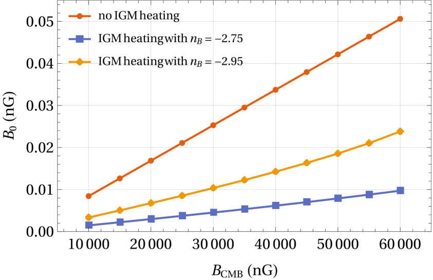
(a) Absolute differences

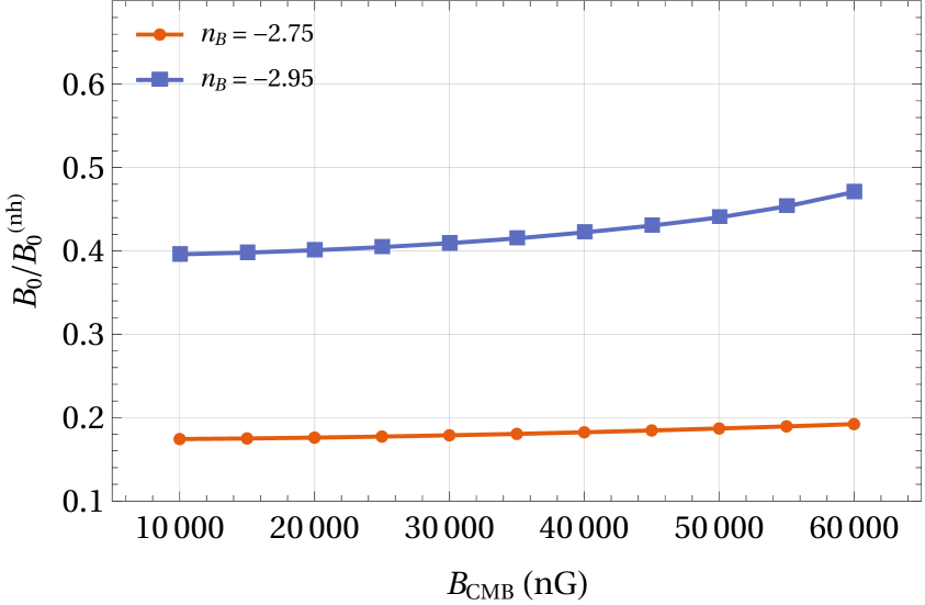
(b) Relative suppression ratio

Figure 2: Difference between the values of the present day magnetic field strength ($B_{0}$) in presence and absence of IGM heating effects via ambipolar diffusion (AD) and decaying turbulence (DT), corresponding to the same set of representative field strengths at recombination ($B_{\rm CMB}$). This shows the significant impact of heating effects on the redshift evolution of weak non-helical PMFs. In the right panel, $B_{0}^{\rm(nh)}$ denotes the case without IGM heating.

In the final step, we use the obtained $B_{0}$ to compute $P_{m}^{(B)}(k)$ using Eq. (2.15), and subsequently calculate the modified SFRD as a function of redshift using Eq. (2.3). Finally, we solve the full system of equations with the modified SFRD in place, and proceed to compute $\overline{T}_{21}(z)$ to compare with the observed global 21-cm dip reported by EDGES [47]. A non-helical PMF alone, due to its heating effect, makes the global 21-cm dip shallower and leads to a worsened discrepancy with observations compared to vanilla $\Lambda$CDM. However, an excess extra-galactic radio background [99], supported by ARCADE-2 [61] and LWA1 [62], provides an effective cooling effect and is known to be capable of extending the $\overline{T}_{21}$ dip downward inside the observed bounds from EDGES [100]. This excess radio background profile can be modelled as [61]

$$T(\nu)=T_{\rm CMB}+\xi T_{R}\left(\frac{\nu}{\nu_{0}}\right)^{\beta},$$ (3.1)

with $T_{R}=1.19\pm 0.14$ K, $\beta=-2.62\pm 0.04$ and $\nu_{0}=1$ GHz being the fitting parameters and $\xi$ being the fraction of excess radiation considered in the process [72].

In the present analysis, we compute the full redshift profiles of $\overline{T}_{21}(z)$ corresponding to two benchmark values of the magnetic spectral index $n_{\!{}_{B}}=-2.75$ and $n_{\!{}_{B}}=-2.95$ (which represent a nearly scale-invariant magnetic power spectrum), considering six different representative values of $\xi=\{0\%,\>2\%,\>5\%,\>10\%,\>15\%,\>20\%\}$. In each case, we show the behaviour of the global 21-cm signal for ten representative values of $B_{\rm CMB}$ ranging from $1.0\times 10^{4}$ nG to $6.0\times 10^{4}$ nG (at incremental steps of $5.0\times 10^{3}$ nG) for $n_{\!{}_{B}}=-2.95$, and from $1.0\times 10^{4}$ nG to $1.0\times 10^{5}$ nG (at incremental steps of $1.0\times 10^{4}$ nG) for $n_{\!{}_{B}}=-2.75$. For the two different values of $n_{\!{}_{B}}$, such different sets of $B_{\rm CMB}$ values have been chosen to better depict the effects on $\overline{T}_{21}(z)$ and obtain upper bounds in light of the EDGES data, as the PMF scale-dependence plays a crucial role in the dynamics of the AD and DT effects. Incorporating the heating phenomena and star formation, both sets of $B_{\rm CMB}$ values typically correspond to $\mathcal{O}(10^{-3}-10^{-2})$ nG field strengths for $B_{0}$.

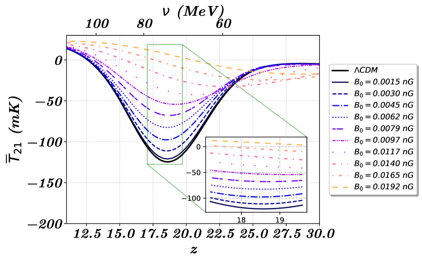
(a) $\xi=0\%$ (absence of excess radio background)

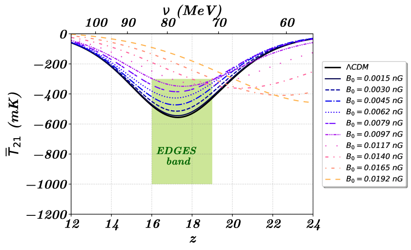
(b) $\xi=2\%$

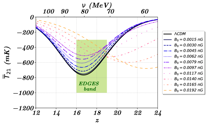
(c) $\xi=5\%$

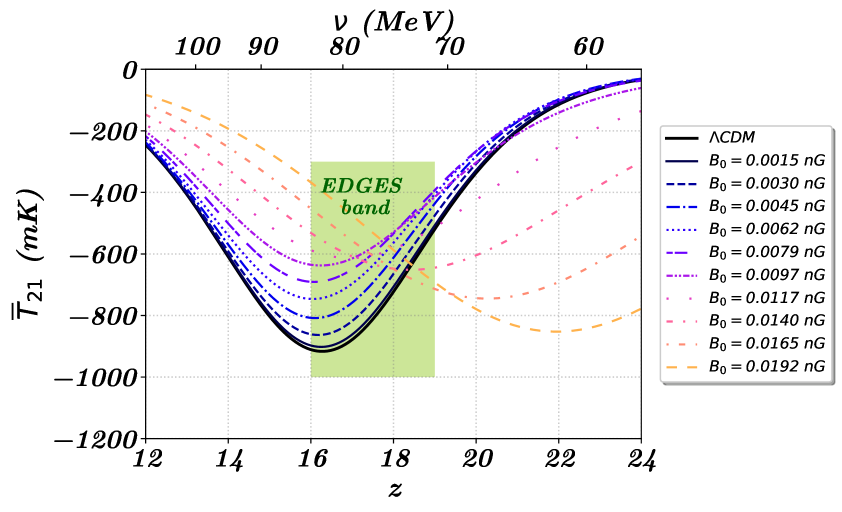
(d) $\xi=10\%$

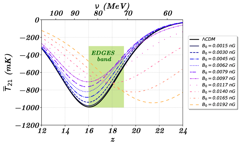
(e) $\xi=15\%$

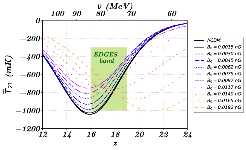
(f) $\xi=20\%$

Figure 3: Global differential brightness temperature for different values of the ARCADE excess radiation parameter ($\xi$), where $\mathbf{n_{\!{}_{B}}=-2.75}$ has been assumed throughout. The EDGES bounds and $\Lambda$CDM plot have been shown for comparison. The quoted values of $B_{0}$ correspond to a set of $B_{\rm CMB}$ values ranging from $1\times 10^{4}$ nG to $1\times 10^{5}$ nG in steps of $1\times 10^{4}$ nG.

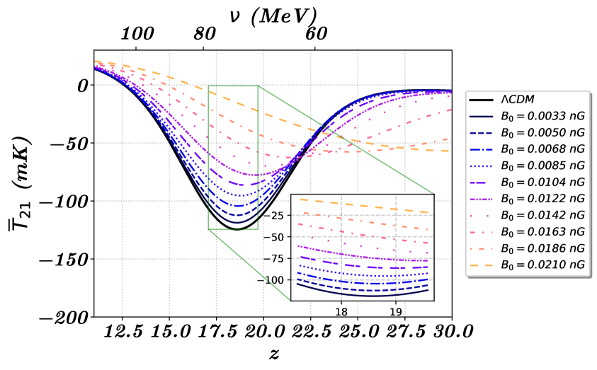
(a) $\xi=0\%$ (absence of excess radio background)

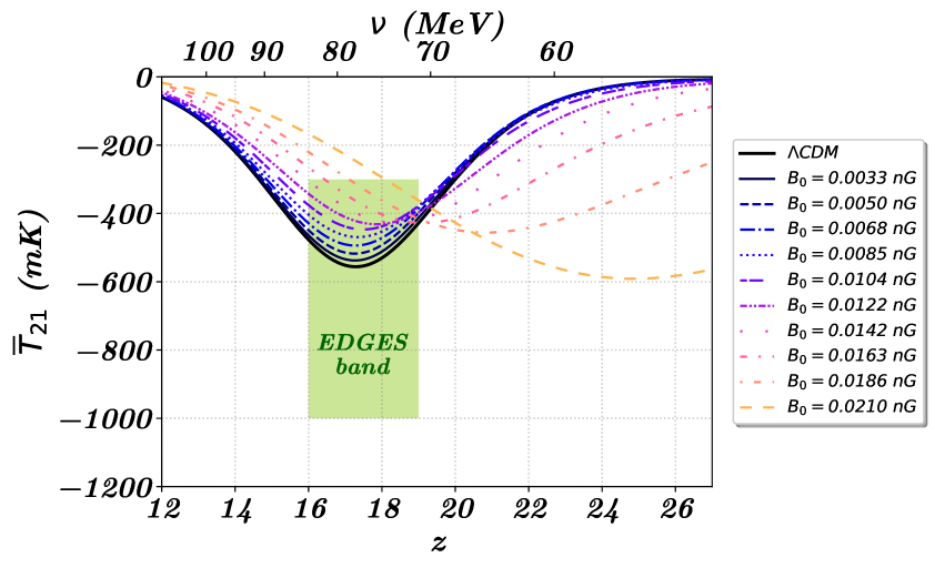
(b) $\xi=2\%$

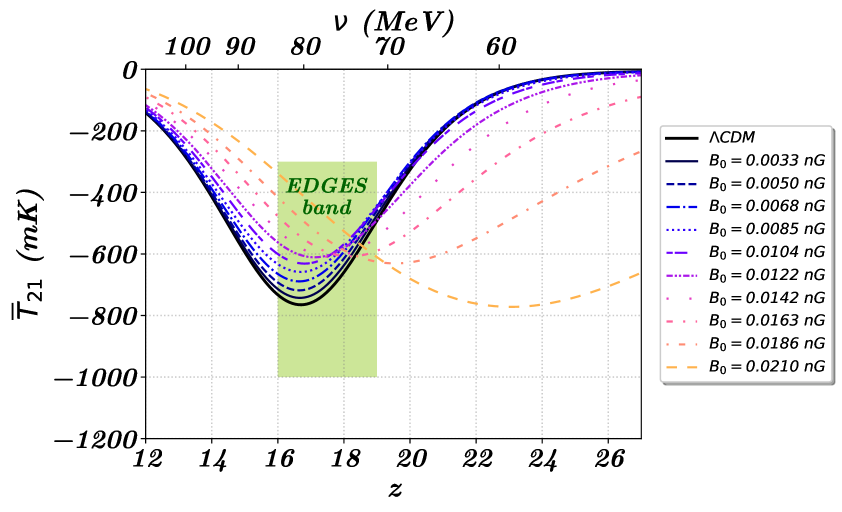
(c) $\xi=5\%$

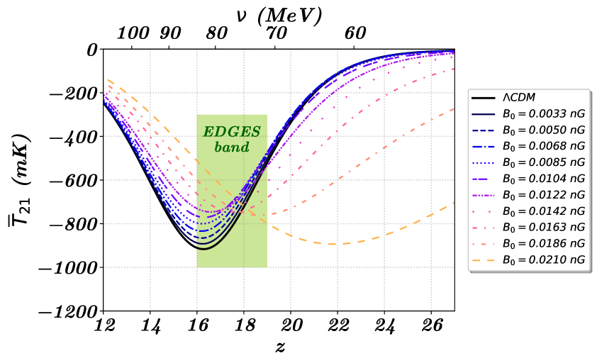
(d) $\xi=10\%$

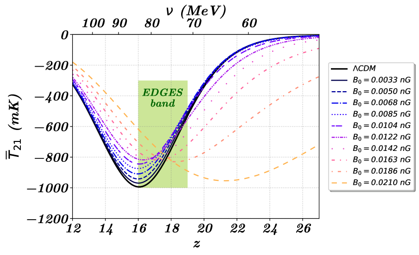
(e) $\xi=15\%$

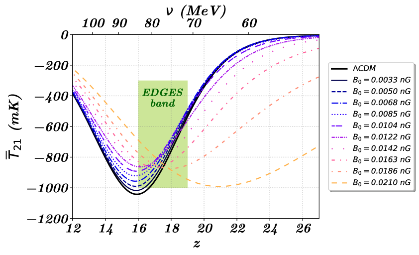
(f) $\xi=20\%$

Figure 4: Global differential brightness temperature for different values of the ARCADE excess radiation parameter ($\xi$), where $\mathbf{n_{\!{}_{B}}=-2.95}$ has been assumed throughout. The EDGES bounds and $\Lambda$CDM plot have been shown for comparison. The quoted values of $B_{0}$ correspond to a set of $B_{\rm CMB}$ values ranging from $1\times 10^{4}$ nG to $6\times 10^{4}$ nG in steps of $5\times 10^{3}$ nG.

The resulting $\overline{T}_{21}(z)$ profiles are shown in Figs. 3 and 4 alongside the observed bounds reported by EDGES [47]. Several interesting features immediately stand out. Firstly, while the IGM heating effects dominate for lower values of $B_{0}$ and gradually raise the 21-cm trough, the effect of enhanced SFRD rapidly becomes prominent as the field strength is increased. The latter induces a sharp lateral shift of the 21-cm trough to progressively earlier redshifts, thereby providing a tighter upper bound on the PMF strength based on the EDGES redshift range $16\lesssim z\lesssim 19$ compared to what can be achieved by considering the heating phenomena alone. The upper bound thus obtained varies between $B_{0}\sim 0.015$ nG and $B_{0}\sim 0.018$ nG as $\xi$ is allowed to vary between $2\%$ and $20\%$, as evident from Figs. 3 and 4. This is nearly two orders of magnitude smaller than the upper bound on $B_{0}$ in the nearly scale-invariant non-helical regime, which has been reported earlier in [53] by considering magnetic heating effects alone. For a fixed value of $n_{\!{}_{B}}$, the upper bound increases slightly for higher values of $\xi$, since excess radio background tends to drag the position of the 21-cm trough to slightly lower redshifts. On the other hand, the admissible upper bound on $B_{0}$ is slightly higher for $n_{\!{}_{B}}=-2.95$ than for $n_{\!{}_{B}}=-2.75$, as seen by comparing Fig. 4 against Fig. 3. Moreover, an interesting interplay of PMFs with the excess radio background profile used in the modelling of ARCADE data [61] becomes apparent at higher redshifts beyond the EDGES band. In absence of any excess radio background, which is indicated by $\xi=0\%$ in Figs. 3(a) and 4(a), the $\overline{T}_{21}$-minima become progressively shallower as they move to higher redshifts with increasing $B_{0}$, as also noted by Ref. [98]. Upon the inclusion of the excess radio profile, however, the “shallowing” of the minima apparently stops at some critical value of $B_{0}$, and all subsequent minima at higher redshifts tend to be deeper. This turning point typically occurs beyond the EDGES redshift range which is of interest to us, with the sole exception of the $\xi=20\%$ case which marginally includes the turning point.

The second interesting feature, which becomes clear upon careful inspection of Figs. 3 and 4, occurs for the smaller values of $B_{0}$ depicted therein. As $B_{0}$ starts to increase and the minima become shallower due to magnetic heating of the IGM, there is a very slight initial leftward shift of the dip to lower redshifts. At first glance, this appears contrary to what one may anticipate, as higher field strengths are expected to enhance early SFRD in our modelling. However, this can be explained on the basis of the redshift-dependence of the magnetically enhanced SFRD, which has been plotted in the right column of Fig. 1 for a few (larger) benchmark values of $B_{0}$. For a given pair of neighbouring values $B_{0}^{(1)}<B_{0}^{(2)}$, the two corresponding SFRD curves cross each other at some particular redshift ($z_{\rm cross}$), with the SFRD for $B_{0}^{(2)}$ being less than that of $B_{0}^{(1)}$ for $z<z_{\rm cross}$. As visible in Fig. 1(d), this crossing takes place at comparatively higher redshifts for weaker field strengths, and occur earlier compared to the EDGES interval for the weakest values of $B_{0}$ depicted in Figs. 3 and 4. Thus, the SFRD slightly decreases in the redshift range $z\lesssim 19$ as $B_{0}$ is increased from the bottom up, resulting in the marginal leftward shift of the 21-cm minima. As $B_{0}$ subsequently increases past a threshold value, the crossing redshift moves to the left of the EDGES interval, and the SFRD subsequently rises in our region of interest with further increase in $B_{0}$, producing the pronounced rightward shift of the dip. While this minute effect is hard to glean from the plots (Figs. 3(a) and 4(a) show zoomed in panels of this region), it is nevertheless significant and plays an important role in determining the correlations among various parameters with respect to their fiducial values, as we investigate in Sec. 5.3.

4 Impact of PMF on the 21-cm power spectrum

Let us now move on to discuss the effects of PMF on the 21-cm power spectrum that would in turn help us in forecasting on the upcoming 21-cm mission SKA-Low. The two-point function for differential brightness temperature fluctuations is defined as [101]

$$\langle\delta T_{21}(\mathbb{k};z)\delta T_{21}(\mathbb{k^{\prime}};z)\rangle\equiv P_{21}(\mathbb{k};z)\delta^{(3)}(\mathbb{k}+\mathbb{k^{\prime}})\>,$$ (4.1)

where $\delta T_{21}(\mathbb{k};z)$ is the Fourier transform of the real-space temperature difference $\delta T_{21}(\mathbb{x};z)\equiv T_{21}(\mathbb{x};z)-\overline{T}_{21}(z)$. Here $P_{21}(\mathbb{k};z)$ represents the 21-cm power spectra which can be modelled analytically as [101]

$$P_{21}(\mathbb{k};z)=\left[\mathcal{A}(z)+\overline{T}_{21}(z)\mu^{2}\right]^{2}P_{\rm HI}(k;z)\>,$$ (4.2)

where $P_{\rm HI}(k;z)$ is the power spectrum of the neutral hydrogen density fluctuations which is approximately equal to the baryon power spectrum $P_{b}(k;z)$ within the redshift range under consideration, $\mu\equiv k_{\parallel}/k$ is the cosine of the angle between the line of sight component ($k_{\parallel}$) and the absolute value ($k$). Furthermore, $\mathcal{A}(z)\equiv\frac{d\overline{T}_{21}(z)}{d\delta_{b}}$ [101, 102] which can be approximated as $\mathcal{A}(z)\approx 2\overline{T}_{21}(z)$ for $z\lesssim 50$ [102], and $\delta_{b}$ is the baryon density fluctuation. For observational purposes, one needs to average over all directions to obtain the 1D power spectrum $P_{21}(k;z)$, which translates to an integral of Eq. (4.2) over $\mu$. The 21-cm power spectrum thus effectively traces the baryon distribution as a function of $k$ with a redshift-dependent bias.

Like the total matter power spectrum, $P_{b}(k;z)$ is similarly enhanced on small scales in presence of PMFs. However, for the typical magnetic field strength which is of interest to us, this enhancement occurs at $k\gtrsim 100$ Mpc^-1, which lies beyond the observable window of next-generation intensity mapping experiments like the Square Kilometre Array (SKA). Hence, limiting our attention to the scales $k\lesssim 10$ Mpc^-1 that are of observational interest, the only effect of PMFs on $P_{21}(k;z)$ arises through $\overline{T}_{21}(z)$. Thus, in our calculations, we make use of the $\overline{T}_{21}(z)$, computed in Sec. 3 and the numerically obtained $P_{b}(k;z)$ from CLASS [103, 104] for each redshift slice.

The $21$-cm power spectrum exhibits a strong dependence on the global signal, indicating that $P_{21}(k;z)$ is enhanced where $\overline{T}_{21}(z)$ shows its minimum. Since a non-helical PMF raises the IGM temperature, the dip in the global signal becomes shallower. Hence, the amplitude of the 21-cm power spectrum decreases upon increasing the magnetic field strength (for some fixed values of $n_{\!{}_{B}}$ and $\xi$), which can be clearly seen in Fig. 5(a). On the other hand, for a given set of parameter values, the depth of the global signal is maximised near $z\sim 16$, which results in an enhancement of power in this redshift region as illustrated in Fig. 5(b).

5 Detection prospects at SKA-Low

The SKA-Low is a phased array of simple dipole antennae covering frequencies ranging from $350$ MHz to $50$ MHz (i.e. $z=4$ to $z=28$) . Since we are interested in the frequency range associated with EDGES ($z\sim\,16-19$), the SKA-Low projection is thus essential for probing the relevant parameters.

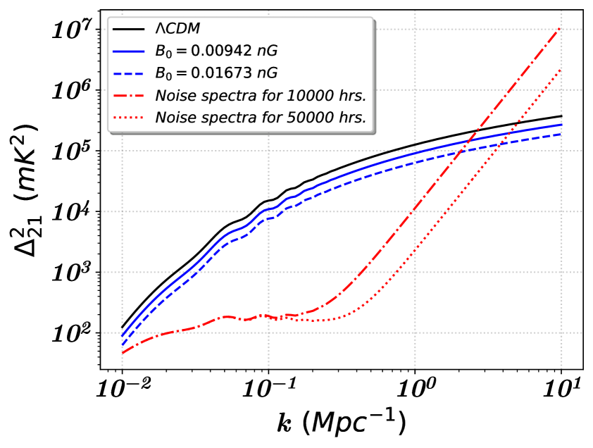
(a) Momentum profiles w.r.t. $B_{0}$ at $z=16$

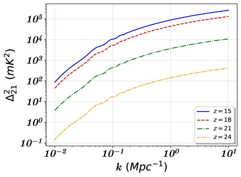
(b) Momentum profiles w.r.t. $z$ for $B_{0}=0.0094$ nG

(c) Redshift profiles w.r.t. $B_{0}$ at $k=0.7$ Mpc^-1

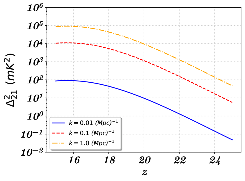
(d) Redshift profiles w.r.t. $k$ for $B_{0}=0.0094$ nG

Figure 5: 21-cm power spectra with SKA-Low noise power spectrum considering cosmic variance and thermal noise. In the upper panel we have depicted the variation of 21-cm power spectra w.r.t. wave-number $k$, whereas the lower panel represents the variation w.r.t. redshift ($z$). In the left panel, we have displayed noise spectra for observation time $10000$ hours and $50000$ hours, and power the spectra compared with $\Lambda$CDM scenario. For each of the plots, we have assumed $n_{\!{}_{B}}=-2.95$ and $\xi=0.20$.

5.1 Noise modelling for SKA-Low

We first elucidate the various sources of noise associated with the observation of the 21-cm power spectrum at SKA-Low. Our investigation takes into account three crucial sources of error that may contaminate the signal: the inherent statistical uncertainty known as cosmic variance, thermal noise, and the instrumental noise of the experimental configuration.

Cosmic variance

Cosmic variance (CV) is an intrinsic source of error due to the availability of only one realisation of the Universe. For 21-cm power spectrum observations, the CV noise is measured in terms of the bin-centred wavenumber $k$ and frequency $\nu$, with bandwidths $\Delta(\ln k)$ and $\Delta\nu$. In our case, we may take $\Delta(\ln k)=1$ and $\Delta\nu=5$ MHz. Considering these, the CV noise can be expressed as [105]

$$P^{\rm N}_{\rm CV}(k;\nu)=\frac{2\pi P_{21}(k,\nu)}{\sqrt{V(\nu)k^{3}\Delta(\ln k)}},$$ (5.1)

where, to calculate $P_{21}(k;\nu)$, we have taken a $\mu$-averaged value of $P_{21}(\mathbb{k};z)$ (Eq. (4.2)) and transformed it to frequency space via the relation $\nu=1420/(1+z)$ MHz. In the expression above, $V(\nu)$ indicates the survey volume for the bin-centered frequency $\nu$ with bandwidth $\Delta\nu$, and be expressed as $V(\nu)=\Omega_{\!{}_{\rm FOV}}r_{\nu}^{2}\Delta r_{\Delta\nu}$. Here, $r_{\nu}$ represents the comoving distance for the bin-centered frequency $\nu$, $\Delta r_{\Delta\nu}$ is the comoving length interval corresponding to the bandwidth $\Delta\nu$, and $\Omega_{\!{}_{\rm FOV}}=\left(0.21(1+z){\rm m}\right)^{2}/A_{\rm eff}$ is the field of view (FOV) with an effective collecting area $A_{\rm eff}=(10^{6}/450)\,{\rm m^{2}}$ [106].

Thermal noise

Thermal noise is also measured in terms of the bin-centered variables $k$ and $\nu$, and can be expressed as [106]

$$P^{\rm N}_{\rm therm}(k;\nu)=\sqrt{\frac{4\,k^{3}\,V(\nu)}{\pi^{2}\,\Delta(\ln k)}}\,\frac{T_{\rm sys}^{2}}{\Delta\nu\,t_{\rm ini}}\,\frac{A_{\rm core}}{N_{\rm st}A_{\rm eff}},$$ (5.2)

where, for SKA-Low, the core area is given by $A_{\rm core}=500^{2}$ m² and the total number of stations is $N_{\rm st}=450$ [106]. The system temperature $T_{\rm sys}$ can be expressed as [107]

$$T_{\rm sys}=180\times\left(\frac{\nu}{180\,\text{MHz}}\right)^{-2.6}\,\text{K}.$$ (5.3)

For the bandwidths $\Delta(\ln k)$ and $\Delta\nu$, we have used the same values as for the CV noise.

Instrumental noise

The instrumental noise for SKA-Low can be expressed in terms of the sky-covering fraction ($f_{\rm cover}$) and the observational period ($t_{o}$) as [108, 109, 110]

$$P^{\rm N}_{\rm ins}(z)=\frac{\pi\,T_{\rm sys}^{2}}{f_{\rm cover}^{2}\,t_{o}}d_{A}^{2}(z)y_{\nu}(z)\frac{\lambda^{2}(z)}{D_{\rm base}^{2}}\>,$$ (5.4)

where $\lambda(z)$ represents the $21$-cm transition wavelength at redshift $z$, and the angular diameter distance can be expressed as $d_{A}(z)=r_{z}/(1+z)$, with $r_{z}$ being the comoving distance at redshift $z$. On the other hand, $y_{\nu}$ is the conversion function from frequency ($\nu$) to $k_{\parallel}$, which can be expressed as [109]

$$y_{\nu}=18.5\times\sqrt{\frac{1+z}{10}}\,\,\text{Mpc/MHz}.$$ (5.5)

For SKA-Low, we have considered a baseline of $D_{\rm base}=1$ km and sky-covering fraction $f_{\rm cover}\approx 0.0091$. Furthermore, we carry out our SNR analysis for two benchmark observation times $t_{o}=10000$ hours and $t_{o}=50000$ hours. The total resulting noise power spectrum can then be written as

$$P^{\rm N}_{21}(k;z)=P^{\rm N}_{\rm CV}(k;z)+P^{\rm N}_{\rm therm}(k;z)+P^{\rm N}_{\rm ins}(z),$$ (5.6)

where the CV and thermal noises are expressed in redshift space by using $\nu=1420/(1+z)$ MHz. From Fig. 5, we observe that CV is the dominant source of noise on large scales, while instrumental noise becomes important at smaller scales. Moreover, the instrumental noise is strong enough to dominate over thermal noise across all scales. Fig. 5 additionally depicts that the instrumental noise scales inversely with the observational time, thereby raising the SNR at smaller scales for longer mission durations.

5.2 Estimation of signal-to-noise ratio (SNR)

For our purpose, the SNR may be defined as an explicit function of both $k$ and $z$ as

$${\rm SNR}\equiv\frac{P_{21}(k;z)}{P_{21}^{\rm N}(k;z)}\>,$$ (5.7)

to arrive at which, we have first performed $\mu$-averaging of $P_{21}(\mathbb{k};z)$ to obtain $P_{21}(k;z)$ (viz. Eq. (4.2)). For a given set of $\{B_{0},n_{\!{}_{B}},\xi\}$, the SNR is found to depend strongly on both $k$ and $z$. This is shown in Fig. 6, which represents the SNR of the 21-cm power spectrum at SKA-Low in the $k$-$z$ plane corresponding to the benchmark parameter values $B_{0}=0.00942$ nG, $n_{\!{}_{B}}=-2.95$, and $\xi=15\%$. As visible in the plot, the SNR peaks close to $z\sim 16$ and in the range $k\in(0.1,1.0)$. The origin of this feature can be traced back to Fig. 4, which displays that the global signal has a trough around $z\sim 16$, which causes an enhancement in the power spectrum near $z\sim 16$ (viz. Fig. 5(b)) and results in a corresponding rise in the SNR. As for the $k$-range, the noise level is significant both at small $k$ (due to CV) and at large $k$ (due to instrumental noise) as might be gleaned from viz. Fig. 5(a), which results in an enhancement of the SNR in the mid-$k$ region. We also compare the SNR for $t_{o}=10000$ hours (Fig. 6(a)) and $t_{o}=50000$ hours (Fig. 6(b)), which shows that the SNR increases nearly one order of magnitude for the longer observational period. This manifests especially at large $k$ due to lesser instrumental noise levels, as evident from Eq. (5.4).

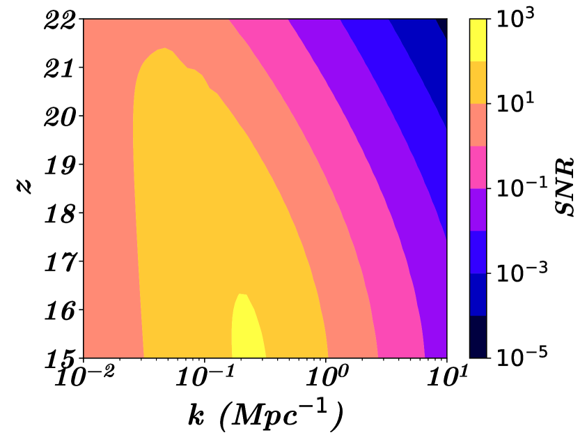
(a) $t_{o}=10000$ hours

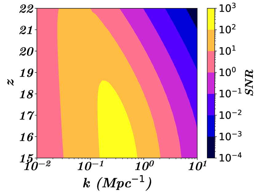
(b) $t_{o}=50000$ hours

Figure 6: Dependence of SNR on wavenumber ($k$) and redshift ($z$) for SKA-Low, considering $B_{0}=0.00942$ nG and $n_{\!{}_{B}}=-2.95$. Left plot displays the scenario for observation time $(t_{o})=10000$ hours, whereas right plot is for $t_{o}=50000$ hours. Both of the figures depicts the instrumental noise along with cosmic variance and thermal noise.

The dependence of SNR on the parameters $\{B_{0},n_{\!{}_{B}},\xi\}$ themselves, on the other hand, is depicted in Fig. 7, which displays the SNR in the $B_{0}$-$\xi$ plane for the two values of $n_{\!{}_{B}}=-2.75$ (Fig. 7(a)) and $n_{\!{}_{B}}=-2.95$ (Fig. 7(b)), corresponding to fixed $k=0.3$ Mpc^-1 and $z=16$. The SNR is found to be maximised for the least value of $B_{0}$ and the highest value of $\xi$. This is in tune with the fact that the PMF heats the gas and attenuates the global signal for larger $B_{0}$, which, in turn, dampens the 21-cm power spectrum. On the other hand, a stronger excess radio background increases the depth of the global signal, resulting in an increment of power.

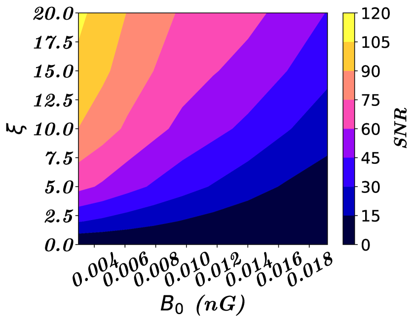
(a) $n_{\!{}_{B}}=-2.75$

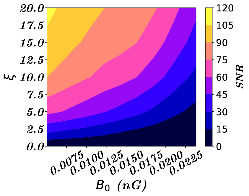
(b) $n_{\!{}_{B}}=-2.95$

Figure 7: Dependence of SNR on magnetic field ($B_{0}$) and $\xi$ for SKA-Low, considering $k=0.3$ Mpc^-1 and $z=16$. Left plot represents $n_{\!{}_{B}}=-2.75$, whereas right plot is for $n_{\!{}_{B}}=-2.95$. Both of the figures depicts the instrumental noise along with cosmic variance and thermal noise. The figures correspond to observation time $t_{o}=50000$ hours.

5.3 Fisher forecast analysis

While the SNR provides a decent idea of the parameter range needed for robust detection, the standard Fisher forecast methodology (with the noise model described in Sec. 5.1) is implemented in this section to assess the experimental capability of SKA-Low in constraining the PMF parameters ($B_{0}$ and $n_{\!{}_{B}}$) jointly with the excess radio background parameter ($\xi$). For maximum likelihood analysis, the standard prescription is to maximise the log-likelihood function ($\mathcal{L}$), in terms of which the Fisher matrix is defined as [111]

$$F_{ab}=\left\langle-\,\frac{\partial^{2}\mathcal{L}(\mathbb{\Theta})}{\partial\Theta_{a}\partial\Theta_{b}}\right\rangle,$$ (5.8)

where $\{\Theta_{i}\}$ indicates the vector of model parameters, with angular brackets representing the angular average over the observational data.

For SKA-Low which is expected to probe $3\lesssim z\lesssim 28$, we consider a mock cosine-averaged $z$-binned 1D power spectrum dataset at a constant $k$-slice. Specifically, the $\mu$-averaged $P_{21}(k,z)$ at a fixed benchmark value of $k=0.3$ Mpc^-1 has been considered as a function of the redshift, with $z$-binnings in accordance with the instrumental specifications of SKA-Low. This is similar to a tomographic study of the 21-cm power spectrum with SKA-Low [112, 113, 114, 115] at a fixed scale. In terms of the noise model, the log-likelihood function for SKA-Low then involves a sum over all the redshift bins, and can be expressed as [116]

$$\mathcal{L}(\mathbb{\Theta};k,z)=\dfrac{f_{\rm sky}}{2}\sum\limits_{i}\int_{-1}^{1}\!\!\!\mathrm{d}\mu\>\frac{\left(P_{21}(k,z_{i},\mu,\mathbb{\Theta})-P_{21}^{\rm fid}(k,z_{i},\mu,\mathbb{\Theta}_{\rm fid})\right)^{2}}{\left(P_{21}(k,z_{i},\mu,\mathbb{\Theta})+P_{21}^{N}(z_{i})\right)^{2}}.$$ (5.9)

Using this in Eq. (5.8), the Fisher matrix is given by

$$F_{ab}(z)=\dfrac{f_{\rm sky}}{2}\sum\limits_{i}\int_{-1}^{1}\!\!\!\mathrm{d}\mu\left[P_{21}(\mathbb{k},z,\mathbb{\Theta})+P_{21}^{N}(z)\right]^{-2}\dfrac{\partial P_{21}(\mathbb{k},z,\mathbb{\Theta})}{\partial\Theta_{a}}\dfrac{\partial P_{21}(\mathbb{k},z,\mathbb{\Theta})}{\partial\Theta_{b}}.$$ (5.10)

For the present analysis, a sky fraction of $f_{sky}=0.72$ has been assumed (corresponding to a cosmological mask [117]), alongside a runtime of $t_{o}=50000$ hours. Equipped with Eq. (5.10), we now proceed to estimate the $1\sigma$ uncertainties on $\{B_{0},n_{\!{}_{B}},\xi\}$ with SKA-Low.

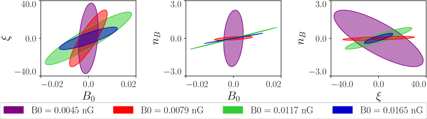
(a) $n_{\!{}_{B}}=-2.75$

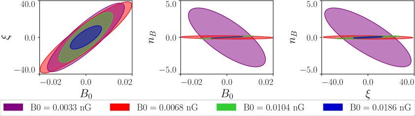
(b) $n_{\!{}_{B}}=-2.95$

Figure 8: Marginalised $1\sigma$ contours of the 2D posterior distribution from Fisher matrix analysis for SKA-Low, considering $\xi=15\%$. To highlight the correlations, actual fiducial positions have not been displayed. The left plot represents the scenario for $n_{\!{}_{B}}=-2.75$, whereas the right one is for $n_{\!{}_{B}}=-2.95$.

Figs. 8, 9, and 10 depict the predicted 2D posterior distributions (at $1\sigma$) for different fiducial values of the parameters (actual fiducial positions have not been displayed to compare the correlations). To plot these results, we have used the plotting library of the publicly available Fisher analysis code CosmicFish [118, 119]. Fig. 8 illustrates the comparisons among the uncertainties associated with different magnetic field strengths for given fiducial values of $\xi=15\%$ and $n_{\!{}_{B}}=-2.75$ ($n_{\!{}_{B}}=-2.95$) in Fig. 8(a) (Fig. 8(b)). In the $B_{0}$-$\xi$ plane, the uncertainties turn out to be strongly positive correlated for $B_{0}=0.0117$ nG for $n_{\!{}_{B}}=-2.75$, whereas the correlation decreases for both $B_{0}>0.0117$ nG and $B_{0}<0.0117$ nG. This feature is more prominent as the magnetic field becomes relatively more scale-dependent i.e. for more positive values of $n_{\!{}_{B}}$. On top of this, the uncertainty associated with $B_{0}=0.0117$ nG is larger. Furthermore, in the $B_{0}$-$n_{\!{}_{B}}$ plane, $B_{0}=0.0117$ nG shows a strong positive correlation with maximum uncertainty among all the fiducial values considered. For $n_{\!{}_{B}}=-2.95$, on the other hand, the dependence of the correlation strength in the $B_{0}$-$\xi$ plane on the fiducial value of $B_{0}$ is observed to be lesser, while similar flips in the correlation are observed at some critical value of $B_{0}$ in the $B_{0}-n_{\!{}_{B}}$ and $\xi-n_{\!{}_{B}}$ planes.

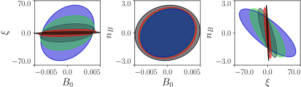
(a) For $B_{0}=0.0045$ nG

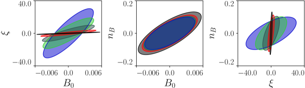
(b) For $B_{0}=0.0079$ nG

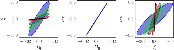
(c) For $B_{0}=0.0117$ nG

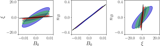
(d) For $B_{0}=0.0165$ nG

Figure 9: Marginalised $1\sigma$ contours of 2D posterior distribution from Fisher matrix analysis for SKA-Low, considering $\mathbf{n_{\!{}_{B}}=-2.75}$. To highlight the correlations, actual fiducial positions have not been displayed.

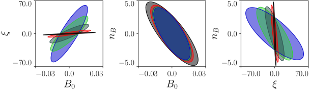
(a) For $B_{0}=0.0033$ nG

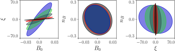
(b) For $B_{0}=0.0068$ nG

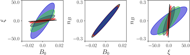
(c) For $B_{0}=0.0104$ nG

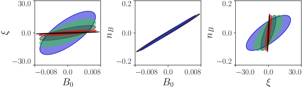
(d) For $B_{0}=0.0186$ nG

Figure 10: Marginalised $1$-$\sigma$ contours of 2-D posterior distribution from Fisher matrix analysis for SKA-Low, considering $\mathbf{n_{\!{}_{B}}=-2.95}$. To highlight the correlations, actual fiducial positions are not displayed.

We have also compared the uncertainties associated with the different values of $\xi$ for several fiducial values of $B_{0}$ and $n_{\!{}_{B}}$, which have been depicted in Figs. 9 (for $n_{\!{}_{B}}=-2.75$) and 10 (for $n_{\!{}_{B}}=-2.95$). Both of the figures represent that $B_{0}$ and $\xi$ are positively correlated for every $B_{0}$ and $n_{\!{}_{B}}$, which is expected since they provide mutually antagonistic effects on $\overline{T}_{21}(z)$. Moreover, $B_{0}$ and $n_{\!{}_{B}}$ are in strong positive correlation for relatively large magnetic field strengths, whereas the correlation vanishes for smaller fields and ultimately switches to negative for sufficiently small magnetic fields. The latter feature is more prominent as $n_{\!{}_{B}}\to-3$, which is why Fig. 10 shows a transition from positive to negative correlation in the $B_{0}-n_{\!{}_{B}}$ plane as $B_{0}$ decreases. The $\xi-n_{\!{}_{B}}$ plane also exhibits the same transition as the magnetic field strength falls.

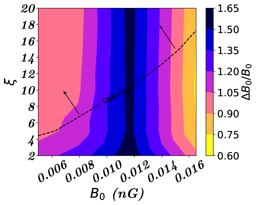
(a)

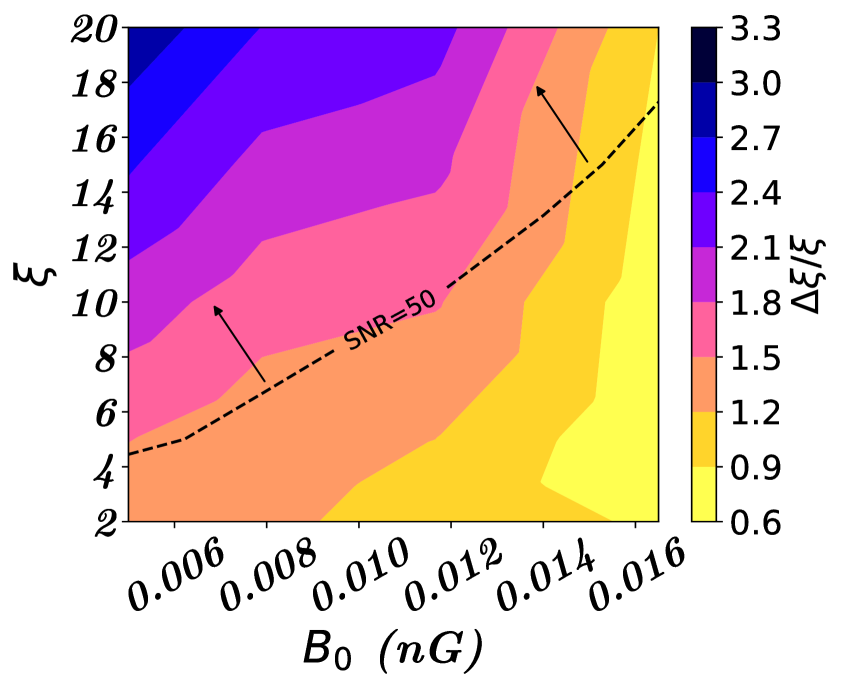
(b)

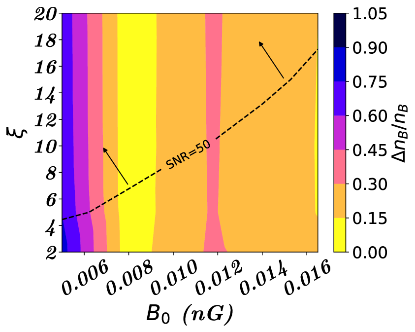
(c)

Figure 11: Variation of relative errors in the $B_{0}$-$\xi$ plane for $\mathbf{n_{\!{}_{B}}=-2.75}$. The black dashed line represents the SNR = 50 contour for $n_{\!{}_{B}}=-2.75$, with arrows indicating the increasing direction of SNR. The figures correspond to the observational time $t_{o}=50000$ hours.

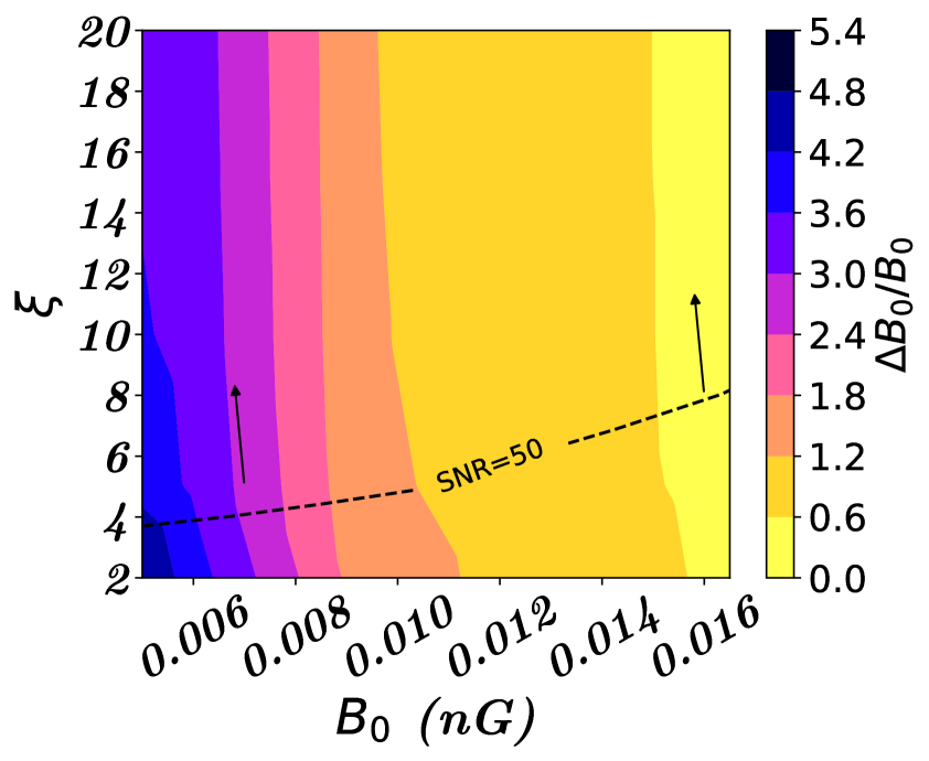
(a)

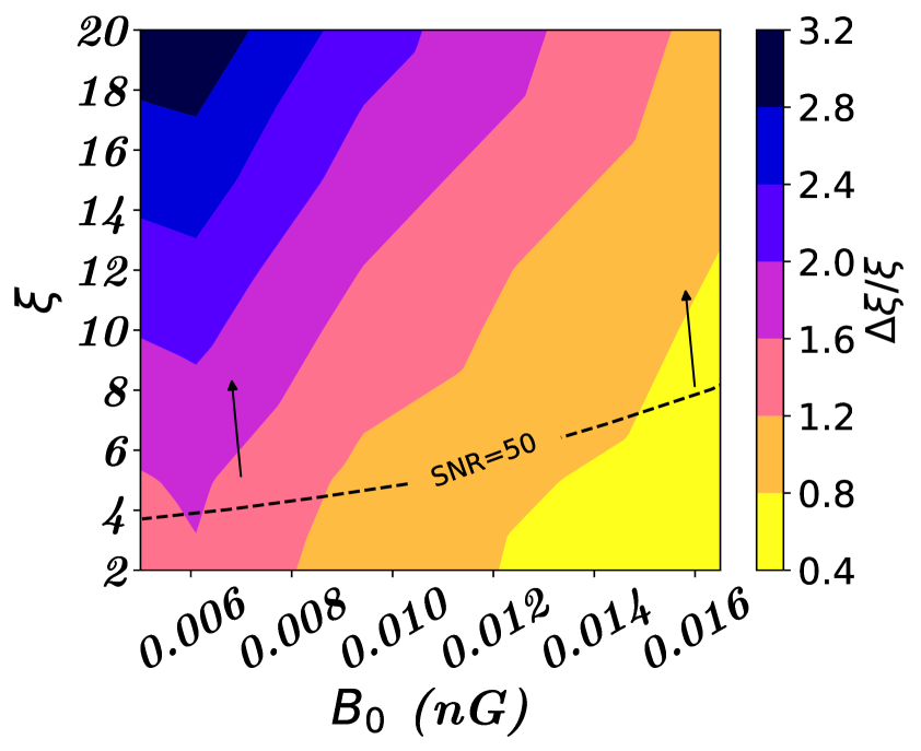
(b)

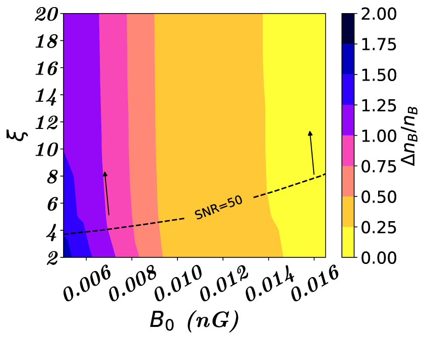
(c)

Figure 12: Variation of relative errors in the $B_{0}$-$\xi$ plane for $\mathbf{n_{\!{}_{B}}=-2.95}$. The black dashed line represents the SNR = 50 contour for $n_{\!{}_{B}}=-2.95$, with arrows indicating the increasing direction of SNR. The figures correspond to the observational time $t_{o}=50000$ hours.

Finally, as Fisher results are inherently dependent on the choice of fiducials, the behaviour of the relative $1\sigma$ uncertainties is displayed in Figs. 11 (for $n_{\!{}_{B}}=-2.75$) and 12 (for $n_{\!{}_{B}}=-2.95$) as functions of the fiducial values. In the plots, we also show the contour for SNR $=50$ for reference (black dashed line). These contour maps indicate that particular regions of the parameter space, where the relative $1\sigma$ uncertainties associated with the various parameters are less than $10\%$, should fall within the detectable threshold of SKA-Low.

6 Summary and future directions

In this article we have investigated the effects of PMF on the global 21-cm signal as well as on the 21-cm power spectrum in a thorough, consistent manner, and found out possible reflections on the relevant observations. Our work consists of two major parts. In the first part, we have investigated possible bounds on PMF parameters based on the global 21-cm signal observed by EDGES, by integrating both IGM heating effects (AD and DT) and PMF-induced modification of the matter power spectrum within a unified framework. The former controls only the vertical height of the global 21-cm trough, whereas the latter impacts the star formation history thereby reflecting on the redshift of the dip. These two effects are usually considered separately in the literature, resulting in their inherent limitations. Our work presents a more comprehensive view by simultaneously addressing these two effects in light of the EDGES signal. The combined impact of both phenomena makes the behaviour of $\overline{T}_{21}(z)$ depart significantly from scenarios where either effect is considered alone. Additionally, we have considered an excess radio background (characterized by $\xi$) on top of the PMF parameter space ($B_{0}$ and $n_{\!{}_{B}}$), with the former providing the essential IGM cooling effect. Our work reveals that the upper bound on $B_{0}$ for a nearly scale-invariant, non-helical PMF should be typically around $\mathcal{O}(10^{-2})$ nG for different choices of the parameters $n_{\!{}_{B}}$ and $\xi$, which is tighter than the previously reported values. We also emphasize that due to AD and DT, the evolution of the magnetic field amplitude should deviate from the trivial adiabatic evolution given by $B(z)=B_{0}(1+z)^{2}$, which has been assumed in some of the earlier works. This issue has been properly addressed through our adopted methodology. Interestingly, as $B_{0}$ starts increasing from zero, a marginal leftward shift of the global 21-cm trough to lower redshifts is observed, whereafter it visibly moves rightward upon further increasing the field strength. The precise reason is that the SFRD curves for distinct values of $B_{0}$ may exhibit crossings with each other at redshifts higher than the interval relevant to EDGES. This, in turn, leads to interesting trends in the correlations among the various parameters.

In the second half of our work, we have turned towards the prospects of detection of effects of PMF on the the 21-cm power spectrum from the future SKA-Low facility. The magnitude of the $\overline{T}_{21}$ dip was found to have significantly influenced the amplitude of the 21-cm power spectrum. With the minimum of $\overline{T}_{21}(z)$ occurring at $z\sim 16-19$, the power at a constant $z$ value (chosen to be $z=16$ for demonstration) gets dampened upon increasing $B_{0}$ for a fixed value of $\xi$, as it leads to a shallower dip. On the other hand, the power at a fixed $z$ rises with increasing $k$ for any given value of $B_{0}$, $n_{\!{}_{B}}$, and $\xi$. Considering possible sources of noise for SKA-Low, it was found that, away from both the high and low-$k$ ends, the $k\in(0.1,1.0)$ Mpc^-1 zone is mostly signal dominated, resulting in an SNR as high as $\mathcal{O}(10^{2})$ at times. Further, to estimate the projected uncertainties associated with the three parameters $\{B_{0},n_{\!{}_{B}},\xi\}$ at SKA-Low, Fisher forecast analysis has been carried out for all of them. Our results shed light on the expected $1\sigma$ errors as well as on the mutual correlations among these three parameters, which show certain interesting trends and may be attributed to various physical processes involved. The error forecasts lead to encouraging results where it seems possible to constrain particular regions of the parameter space with a relative error $\lesssim 10\%$ and SNR $\gtrsim 10$.

To wrap things up, this paper is an attempt at a comprehensive analytical study of the bounds on non-helical, nearly scale-invariant PMFs, that are achievable based on pre-reionization 21-cm physics ($z\sim 15-25$) via the current EDGES observation and an upcoming 21-cm facility like the SKA-Low. Interesting possibilities in view of PMFs also exist well outside this redshift range towards both higher and lower ends. In particular, the 21-cm signal from the dark ages spanning $z\sim 30-100$ is expected to be a pristine source of cosmological information [120], being free from the astrophysical uncertainties associated with stellar processes at lower redshifts. The prospects of constraining PMFs based on the global signal from the dark ages have recently been explored in Ref. [121]. On the other hand, EoR and post-EoR physics may provide independent bounds on the PMF parameters, as investigated earlier in Refs. [122, 123]. As a possible future direction, it is worth re-investigating these scenarios in a joint manner based on our combined analysis, alongside the inclusion of additional current and future datasets, e.g. from CMB and baryon acoustic oscillations (BAO), hence forecasting on the synergy of future cosmological missions when it comes to constraining the PMF parameters. We plan to address some of these possibilities in our upcoming works.

Appendix A Discussion on HI and HeI ionization fractions

In this appendix, we discuss the modelling of the ionization fractions of HI and HeI, according to Ref. [86]. This leads to the evolution of proton fraction and singly ionized helium fraction which has been shown in Eqs. (2.1) and (2.1), respectively.

In the above set of equations, $\alpha$, Case-B recombination coefficient, has different fitting forms for HI and HeI. For HI, it can be expressed as [124, 125]

$$\alpha_{\rm H}\equiv F\times 10^{-19}\frac{at^{b}}{1+ct^{d}}\,\,\mathrm{m^{3}s^{-1}},$$ (A.1)

with $a=4.309$, $b=-0.6166$, $c=0.6703$, $d=0.5300$, $F=1.14$ and $t\equiv T_{k}/10^{4}\,$K. On the other hand, for HeI, it is given by [126]

$$\alpha_{\rm He}\equiv q\left[\sqrt{T_{k}\over T_{2}}\left(1+\sqrt{T_{k}\over T_{2}}\right)^{1-p}\left(1+\sqrt{T_{k}\over T_{1}}\right)^{1+p}\right]^{-1}\,\mathrm{m^{3}s^{-1}},$$ (A.2)

with $q=10^{-16.744}$, $p=0.711$, $T_{1}=10^{5.114}\,$K, and $T_{2}=3\,$K. We have denoted the photoionization coefficient by $\beta$ in Eqs. (2.1) and (2.1) (suffix carries the usual meaning), which can be expressed in terms of $\alpha$ as [86]

$$\beta\equiv\alpha\,\left(2\pi\,m_{e}\,k_{\!{}_{B}}\,T_{k}/h_{P}^{2}\right)^{3/2}\exp{\left(\frac{-h_{P}\,\nu_{2s}}{k_{\!{}_{B}}T_{k}}\right)},$$ (A.3)

with $m_{e}$ being the electron mass.

The cosmological redshifting of HI Ly-$\alpha$ photons and HeI $2^{1}p-1^{1}s$ photons are denoted respectively by $K_{\rm H}\equiv\frac{\lambda^{3}_{\rm H}}{8\pi\,H(z)}$ and $K_{\rm He}\equiv\frac{\lambda^{3}_{\rm He}}{8\pi\,H(z)}$ [86]. As for the specific values of the parameters involved at this point, we have used the atomic data given in Tab. 1 .

Quantities	Physical meaning	Values
$\lambda_{H2p}$	H Ly-$\alpha$ wavelength	$121.5682$ nm
$\lambda_{He}$	He $2^{1}p-1^{1}s$ wavelength	$58.4334$ nm
$\nu_{H2s}$	H $2s-1p$ frequency	$3.29\times 10^{15}$ Hz
$\nu_{He2^{1}s}$	He $2^{1}s-1^{1}s$ frequency	$5\times 10^{15}$ Hz
$\Lambda_{\rm H}$	H $2s-1s$ two photon rate	$8.22458$ s-1
$\Lambda_{\rm He}$	He $2^{1}s-1^{1}s$ two photon rate	$51.3$ s-1
$f_{\!{}_{\rm He}}$	number of helium fraction	$0.08$

Table 1: A list of the atomic data used to explain the ionization history, following Ref. [86].

.

References

- [1] P. Blasi, S. Burles and A.V. Olinto, Cosmological Magnetic Field Limits in an Inhomogeneous Universe, The Astrophysical Journal 514 (1999) L79.
- [2] T. Akahori and D. Ryu, Faraday Rotation Measure due to the Intergalactic Magnetic Field, The Astrophysical Journal 723 (2010) 476.
- [3] T. Vernstrom, B.M. Gaensler, L. Rudnick and H. Andernach, Differences in Faraday Rotation between Adjacent Extragalactic Radio Sources as a Probe of Cosmic Magnetic Fields, The Astrophysical Journal 878 (2019) 92.
- [4] S.P. O’Sullivan et al., New constraints on the magnetization of the cosmic web using LOFAR Faraday rotation observations, Monthly Notices of the Royal Astronomical Society 495 (2020) 2607.
- [5] J.D. Barrow, P.G. Ferreira and J. Silk, Constraints on a Primordial Magnetic Field, Phys. Rev. Lett. 78 (1997) 3610.
- [6] T.R. Seshadri and K. Subramanian, Cosmic Microwave Background Bispectrum from Primordial Magnetic Fields on Large Angular Scales, Phys. Rev. Lett. 103 (2009) 081303.
- [7] Planck collaboration, Planck 2015 results. XIX. Constraints on primordial magnetic fields, Astron. Astrophys. 594 (2016) A19 [1502.01594].
- [8] A. Neronov and I. Vovk, Evidence for Strong Extragalactic Magnetic Fields from Fermi Observations of TeV Blazars, Science 328 (2010) 73.
- [9] K. Dolag, M. Kachelriess, S. Ostapchenko and R. Tomàs, Lower limit on the strength and filling factor of extragalactic magnetic fields, The Astrophysical Journal Letters 727 (2010) L4.
- [10] P. Tiede et al., Constraints on the Intergalactic Magnetic Field from Bow Ties in the Gamma-Ray Sky, The Astrophysical Journal 892 (2020) 123.
- [11] L.M. Widrow, Origin of galactic and extragalactic magnetic fields, Rev. Mod. Phys. 74 (2002) 775.
- [12] A. Brandenburg and E. Ntormousi, Galactic Dynamos, 2211.03476.
- [13] R. Beck, L. Chamandy, E. Elson and E.G. Blackman, Synthesizing Observations and Theory to Understand Galactic Magnetic Fields: Progress and Challenges, Galaxies 8 (2019) 4 [1912.08962].
- [14] S. Bertone, C. Vogt and T. Enßlin, Magnetic field seeding by galactic winds, Monthly Notices of the Royal Astronomical Society 370 (2006) 319.
- [15] B. Ratra, Cosmological “Seed” Magnetic Field from Inflation, The Astrophysical Journal Letters 391 (1992) L1.
- [16] J. Martin and J. Yokoyama, Generation of Large-Scale Magnetic Fields in Single-Field Inflation, JCAP 01 (2008) 025 [0711.4307].
- [17] R.J.Z. Ferreira, R.K. Jain and M.S. Sloth, Inflationary magnetogenesis without the strong coupling problem, JCAP 10 (2013) 004 [1305.7151].
- [18] F.A. Membiela, Primordial magnetic fields from a non-singular bouncing cosmology, Nucl. Phys. B 885 (2014) 196 [1312.2162].
- [19] R. Sharma, S. Jagannathan, T.R. Seshadri and K. Subramanian, Challenges in inflationary magnetogenesis: Constraints from strong coupling, backreaction, and the Schwinger effect, Phys. Rev. D 96 (2017) 083511.
- [20] M.S. Turner and L.M. Widrow, Inflation-produced, large-scale magnetic fields, Phys. Rev. D 37 (1988) 2743.
- [21] K.E. Kunze, Large scale magnetic fields from gravitationally coupled electrodynamics, Phys. Rev. D 81 (2010) 043526.
- [22] P. Qian and Z.-K. Guo, Model of inflationary magnetogenesis, Phys. Rev. D 93 (2016) 043541.
- [23] R. Durrer, L. Hollenstein and R.K. Jain, Can slow roll inflation induce relevant helical magnetic fields?, JCAP 03 (2011) 037 [1005.5322].
- [24] R. Sharma, K. Subramanian and T.R. Seshadri, Generation of helical magnetic field in a viable scenario of inflationary magnetogenesis, Phys. Rev. D 97 (2018) 083503 [1802.04847].
- [25] S. Chakraborty, S. Pal and S. SenGupta, Hilltop Inflation and Generation of Helical Magnetic Field, Universe 8 (2022) 26 [1810.03478].
- [26] J.M. Quashnock, A. Loeb and D.N. Spergel, Magnetic Field Generation During the Cosmological QCD Phase Transition, Astrophys. J. Lett. 344 (1989) L49.
- [27] T. Vachaspati, Magnetic fields from cosmological phase transitions, Phys. Lett. B 265 (1991) 258.
- [28] K. Enqvist and P. Olesen, On primordial magnetic fields of electroweak origin, Phys. Lett. B 319 (1993) 178 [hep-ph/9308270].
- [29] B. Cheng and A.V. Olinto, Primordial magnetic fields generated in the quark-hadron transition, Phys. Rev. D 50 (1994) 2421.
- [30] G. Baym, D. Bödeker and L. McLerran, Magnetic fields produced by phase transition bubbles in the electroweak phase transition, Phys. Rev. D 53 (1996) 662.
- [31] G. Sigl, A.V. Olinto and K. Jedamzik, Primordial magnetic fields from cosmological first order phase transitions, Phys. Rev. D 55 (1997) 4582 [astro-ph/9610201].
- [32] M. Hindmarsh and A. Everett, Magnetic fields from phase transitions, Phys. Rev. D 58 (1998) 103505 [astro-ph/9708004].
- [33] T. Kahniashvili, A.G. Tevzadze, A. Brandenburg and A. Neronov, Evolution of Primordial Magnetic Fields from Phase Transitions, Phys. Rev. D 87 (2013) 083007 [1212.0596].
- [34] J. Ellis, M. Fairbairn, M. Lewicki, V. Vaskonen and A. Wickens, Intergalactic Magnetic Fields from First-Order Phase Transitions, JCAP 09 (2019) 019 [1907.04315].
- [35] M.O. Olea-Romacho, Primordial magnetogenesis in the two-Higgs-doublet model, Phys. Rev. D 109 (2024) 015023 [2310.19948].
- [36] R. Durrer and A. Neronov, Cosmological magnetic fields: their generation, evolution and observation, The Astronomy and Astrophysics Review 21 (2013) 62.
- [37] K. Subramanian, The origin, evolution and signatures of primordial magnetic fields, Reports on Progress in Physics 79 (2016) 076901.
- [38] K. Jedamzik, V.c.v. Katalinić and A.V. Olinto, Damping of cosmic magnetic fields, Phys. Rev. D 57 (1998) 3264.
- [39] K. Subramanian and J.D. Barrow, Magnetohydrodynamics in the early universe and the damping of nonlinear alfvén waves, Phys. Rev. D 58 (1998) 083502.
- [40] S.K. Sethi and K. Subramanian, Primordial magnetic fields in the post-recombination era and early reionization, Mon. Not. Roy. Astron. Soc. 356 (2005) 778 [astro-ph/0405413].
- [41] K.E. Kunze and E. Komatsu, Constraining primordial magnetic fields with distortions of the black-body spectrum of the cosmic microwave background: pre- and post-decoupling contributions, JCAP 01 (2014) 009 [1309.7994].
- [42] J. Chluba, D. Paoletti, F. Finelli and J.-A. Rubiño Martín, Effect of primordial magnetic fields on the ionization history, Mon. Not. Roy. Astron. Soc. 451 (2015) 2244 [1503.04827].
- [43] H. Tashiro and N. Sugiyama, Probing Primordial Magnetic Fields with the 21cm Fluctuations, Mon. Not. Roy. Astron. Soc. 372 (2006) 1060 [astro-ph/0607169].
- [44] D.R.G. Schleicher, R. Banerjee and R.S. Klessen, Influence of primordial magnetic fields on 21 cm emission, Astrophys. J. 692 (2009) 236 [0808.1461].
- [45] K.E. Kunze, 21 cm line signal from magnetic modes, JCAP 01 (2019) 033 [1805.10943].
- [46] H.A.G. Cruz, T. Adi, J. Flitter, M. Kamionkowski and E.D. Kovetz, 21-cm fluctuations from primordial magnetic fields, Phys. Rev. D 109 (2024) 023518 [2308.04483].
- [47] J.D. Bowman, A.E.E. Rogers, R.A. Monsalve, T.J. Mozdzen and N. Mahesh, An absorption profile centred at 78 megahertz in the sky-averaged spectrum, Nature 555 (2018) 67 [1810.05912].
- [48] R. Barkana, Possible interaction between baryons and dark-matter particles revealed by the first stars, Nature 555 (2018) 71 [1803.06698].
- [49] T. Minoda, H. Tashiro and T. Takahashi, Insight into primordial magnetic fields from 21-cm line observation with EDGES experiment, Mon. Not. Roy. Astron. Soc. 488 (2019) 2001 [1812.00730].
- [50] J.R. Bhatt, P.K. Natwariya, A.C. Nayak and A.K. Pandey, Baryon-Dark matter interaction in presence of magnetic fields in light of EDGES signal, Eur. Phys. J. C 80 (2020) 334 [1905.13486].
- [51] A. Bera, K.K. Datta and S. Samui, Primordial magnetic fields during the cosmic dawn in light of EDGES 21-cm signal, Mon. Not. Roy. Astron. Soc. 498 (2020) 918 [2005.14206].
- [52] P.K. Natwariya and J.R. Bhatt, EDGES signal in the presence of magnetic fields, Mon. Not. Roy. Astron. Soc. 497 (2020) L35 [2001.00194].
- [53] P.K. Natwariya, Constraint on Primordial Magnetic Fields In the Light of ARCADE 2 and EDGES Observations, Eur. Phys. J. C 81 (2021) 394 [2007.09938].
- [54] M.R. Krumholz and C. Federrath, The Role of Magnetic Fields in Setting the Star Formation Rate and the Initial Mass Function, Frontiers in Astronomy and Space Sciences 6 (2019) 7 [1902.02557].
- [55] P. Sharda, C. Federrath and M.R. Krumholz, The importance of magnetic fields for the initial mass function of the first stars, Mon. Not. Roy. Astron. Soc. 497 (2020) 336 [2002.11502].
- [56] D. Koh, T. Abel and K. Jedamzik, First Star Formation in the Presence of Primordial Magnetic Fields, Astrophys. J. Lett. 909 (2021) L21 [2101.09281].
- [57] L.R. Prole, P.C. Clark, R.S. Klessen, S.C.O. Glover and R. Pakmor, Primordial magnetic fields in Population III star formation: a magnetized resolution study, Mon. Not. Roy. Astron. Soc. 516 (2022) 2223 [2206.11919].
- [58] D.J. Whitworth, R.J. Smith, R.S. Klessen, M.-M. Mac Low, S.C.O. Glover, R. Tress et al., Magnetic fields do not suppress global star formation in low metallicity dwarf galaxies, Monthly Notices of the Royal Astronomical Society 520 (2023) 89 [2210.04922].
- [59] T. Adi, S. Libanore, H.A.G. Cruz and E.D. Kovetz, Constraining primordial magnetic fields with line-intensity mapping, JCAP 09 (2023) 035 [2305.06440].
- [60] M. Sanati, S. Martin-Alvarez, J. Schober, Y. Revaz, A. Slyz and J. Devriendt, Dwarf galaxies as a probe of a primordially magnetized Universe, arXiv e-prints (2024) arXiv:2403.05672 [2403.05672].
- [61] D.J. Fixsen, A. Kogut, S. Levin, M. Limon, P. Lubin, P. Mirel et al., ARCADE 2 Measurement of the Absolute Sky Brightness at 3-90 GHz, The Astrophysical Journal 734 (2011) 5 [0901.0555].
- [62] G.B. Taylor, S.W. Ellingson et al., First Light for the First Station of the Long Wavelength Array, Journal of Astronomical Instrumentation 1 (2012) 1250004 [1206.6733].
- [63] C.L. Carilli and S. Rawlings, Science with the Square Kilometer Array: Motivation, key science projects, standards and assumptions, New Astron. Rev. 48 (2004) 979 [astro-ph/0409274].
- [64] R. Braun, T. Bourke, J.A. Green, E. Keane and J. Wagg, Advancing Astrophysics with the Square Kilometre Array, in Advancing Astrophysics with the Square Kilometre Array (AASKA14), p. 174, Apr., 2015, DOI.
- [65] SKA collaboration, Cosmology with Phase 1 of the Square Kilometre Array: Red Book 2018: Technical specifications and performance forecasts, Publ. Astron. Soc. Austral. 37 (2020) e007 [1811.02743].
- [66] A. Weltman et al., Fundamental physics with the Square Kilometre Array, Publ. Astron. Soc. Austral. 37 (2020) e002 [1810.02680].
- [67] R. Braun, A. Bonaldi, T. Bourke, E. Keane and J. Wagg, Anticipated Performance of the Square Kilometre Array – Phase 1 (SKA1), arXiv e-prints (2019) arXiv:1912.12699 [1912.12699].
- [68] B.M. Gaensler, The square kilometre array: a new probe of cosmic magnetism, Astron. Nachr. 327 (2006) 387 [astro-ph/0603049].
- [69] R. Beck, Magnetic Visions: Mapping Cosmic Magnetism with LOFAR and SKA, Rev. Mex. Astron. Astrof. Ser. Conf. 36 (2009) 1 [0804.4594].
- [70] S. Roy, S. Sur, K. Subramanian, A. Mangalam, T.R. Seshadri and H. Chand, Probing Magnetic Fields with Square Kilometre Array and its Precursors, Journal of Astrophysics and Astronomy 37 (2016) 42 [1611.06966].
- [71] G. Heald, S.A. Mao, V. Vacca, T. Akahori, A. Damas-Segovia, B.M. Gaensler et al., Magnetism Science with the Square Kilometre Array, Galaxies 8 (2020) 53 [2006.03172].
- [72] C. Feng and G. Holder, Enhanced Global Signal of Neutral Hydrogen Due to Excess Radiation at Cosmic Dawn, The Astrophysical Journal Letters 858 (2018) L17 [1802.07432].
- [73] S.R. Furlanetto, S.P. Oh and F.H. Briggs, Cosmology at low frequencies: The 21 cm transition and the high-redshift Universe, Physics Reports 433 (2006) 181 [astro-ph/0608032].
- [74] J.R. Pritchard and A. Loeb, 21 cm cosmology in the 21st century, Reports on Progress in Physics 75 (2012) 086901 [1109.6012].
- [75] G.B. Field, Excitation of the Hydrogen 21-CM Line, Proceedings of the IRE 46 (1958) 240.
- [76] G.B. Field, The Time Relaxation of a Resonance-Line Profile., The Astrophysical Journal 129 (1959) 551.
- [77] M. Kuhlen, P. Madau and R. Montgomery, The Spin Temperature and 21 cm Brightness of the Intergalactic Medium in the Pre-Reionization era, The Astrophysical Journal Letters 637 (2006) L1 [astro-ph/0510814].
- [78] S.R. Furlanetto, S.P. Oh and E. Pierpaoli, Effects of dark matter decay and annihilation on the high-redshift 21cm background, Phys. Rev. D 74 (2006) 103502 [astro-ph/0608385].
- [79] R. Barkana and A. Loeb, Detecting the Earliest Galaxies through Two New Sources of 21 Centimeter Fluctuations, The Astrophysical Journal 626 (2005) 1 [astro-ph/0410129].
- [80] X.-L. Chen and J. Miralda-Escude, The spin - kinetic temperature coupling and the heating rate due to Lyman - alpha scattering before reionization: Predictions for 21cm emission and absorption, Astrophys. J. 602 (2004) 1 [astro-ph/0303395].
- [81] J.R. Pritchard and S.R. Furlanetto, Descending from on high: Lyman-series cascades and spin-kinetic temperature coupling in the 21-cm line, Mon. Not. Roy. Astron. Soc. 367 (2006) 1057 [astro-ph/0508381].
- [82] R. Barkana and A. Loeb, Detecting the earliest galaxies through two new sources of 21cm fluctuations, Astrophys. J. 626 (2005) 1 [astro-ph/0410129].
- [83] A. Schneider, Constraining noncold dark matter models with the global 21-cm signal, Phys. Rev. D 98 (2018) 063021 [1805.00021].
- [84] J.H. Wise, V.G. Demchenko, M.T. Halicek, M.L. Norman, M.J. Turk, T. Abel et al., The birth of a galaxy – III. Propelling reionization with the faintest galaxies, Mon. Not. Roy. Astron. Soc. 442 (2014) 2560 [1403.6123].
- [85] W.H. Press and P. Schechter, Formation of Galaxies and Clusters of Galaxies by Self-Similar Gravitational Condensation, Astrophys. J. 187 (1974) 425.
- [86] S. Seager, D.D. Sasselov and D. Scott, A new calculation of the recombination epoch, Astrophys. J. Lett. 523 (1999) L1 [astro-ph/9909275].
- [87] S. Bharadwaj and S.S. Ali, The cosmic microwave background radiation fluctuations from HI perturbations prior to reionization, Mon. Not. Roy. Astron. Soc. 352 (2004) 142 [astro-ph/0401206].
- [88] A. Chatterjee, P. Dayal, T.R. Choudhury and A. Hutter, Ruling out 3 keV warm dark matter using 21 cm EDGES data, Mon. Not. Roy. Astron. Soc. 487 (2019) 3560 [1902.09562].
- [89] S.C.O. Glover and P.W.J.L. Brand, Radiative feedback from an early X-ray background, Mon. Not. Roy. Astron. Soc. 340 (2003) 210 [astro-ph/0205308].
- [90] K.E. Kunze and E. Komatsu, Constraining primordial magnetic fields with distortions of the black-body spectrum of the cosmic microwave background: pre- and post-decoupling contributions, JCAP 01 (2014) 009 [1309.7994].
- [91] J.R. Shaw and A. Lewis, Massive neutrinos and magnetic fields in the early universe, Phys. Rev. D 81 (2010) 043517.
- [92] J.R. Shaw and A. Lewis, Constraining primordial magnetism, Phys. Rev. D 86 (2012) 043510.
- [93] K.L. Pandey and S.K. Sethi, Theoretical Estimates of Two-point Shear Correlation Functions using Tangled Magnetic Fields, The Astrophysical Journal 748 (2012) 27 [1201.3619].
- [94] K.E. Kunze, CMB and matter power spectra from cross correlations of primordial curvature and magnetic fields, Phys. Rev. D 87 (2013) 103005 [1301.6105].
- [95] T. Adi, H.A.G. Cruz and M. Kamionkowski, Primordial density perturbations from magnetic fields, Phys. Rev. D 108 (2023) 023521 [2306.11319].
- [96] K.E. Kunze, Magnetic field back reaction on the matter power spectrum, JCAP 09 (2022) 047 [2207.09859].
- [97] S.K. Sethi and K. Subramanian, Primordial magnetic fields in the post-recombination era and early reionization, Mon. Not. Roy. Astron. Soc. 356 (2005) 778 [astro-ph/0405413].
- [98] H.A.G. Cruz, T. Adi, J. Flitter, M. Kamionkowski and E.D. Kovetz, 21-cm fluctuations from primordial magnetic fields, Phys. Rev. D 109 (2024) 023518 [2308.04483].
- [99] R. Subrahmanyan and R. Cowsik, Is there an Unaccounted for Excess in the Extragalactic Cosmic Radio Background?, Astrophys. J. 776 (2013) 42 [1305.7060].
- [100] C. Feng and G. Holder, Enhanced global signal of neutral hydrogen due to excess radiation at cosmic dawn, Astrophys. J. Lett. 858 (2018) L17 [1802.07432].
- [101] J.B. Muñoz, Y. Ali-Haïmoud and M. Kamionkowski, Primordial non-gaussianity from the bispectrum of 21-cm fluctuations in the dark ages, Phys. Rev. D 92 (2015) 083508 [1506.04152].
- [102] Y. Ali-Haïmoud, P.D. Meerburg and S. Yuan, New light on 21 cm intensity fluctuations from the dark ages, Phys. Rev. D 89 (2014) 083506 [1312.4948].
- [103] J. Lesgourgues, The Cosmic Linear Anisotropy Solving System (CLASS) I: Overview, arXiv e-prints (2011) arXiv:1104.2932 [1104.2932].
- [104] D. Blas, J. Lesgourgues and T. Tram, The Cosmic Linear Anisotropy Solving System (CLASS). Part II: Approximation schemes, The Astrophysical Journal 2011 (2011) 034 [1104.2933].
- [105] R. Mondal, S. Bharadwaj and S. Majumdar, Statistics of the epoch of reionization 21-cm signal – I. Power spectrum error-covariance, Mon. Not. Roy. Astron. Soc. 456 (2016) 1936 [1508.00896].
- [106] G. Mellema, L.V.E. Koopmans, F.A. Abdalla, G. Bernardi, B. Ciardi, S. Daiboo et al., Reionization and the Cosmic Dawn with the Square Kilometre Array, Experimental Astronomy 36 (2013) 235 [1210.0197].
- [107] A. de Oliveira-Costa, M. Tegmark, B.M. Gaensler, J. Jonas, T.L. Landecker and P. Reich, A model of diffuse Galactic Radio Emission from 10 MHz to 100 GHz, Mon. Not. Roy. Astron. Soc. 388 (2008) 247 [0802.1525].
- [108] M. Zaldarriaga, S.R. Furlanetto and L. Hernquist, 21 Centimeter fluctuations from cosmic gas at high redshifts, Astrophys. J. 608 (2004) 622 [astro-ph/0311514].
- [109] M. Tegmark and M. Zaldarriaga, The Fast Fourier Transform Telescope, Phys. Rev. D 79 (2009) 083530 [0805.4414].
- [110] T. Modak, T. Plehn, L. Röver and B.M. Schäfer, Probing the Inflaton Potential with SKA, SciPost Phys. Core 5 (2022) 037 [2112.09148].
- [111] M. Tegmark, A. Taylor and A. Heavens, Karhunen-Loeve eigenvalue problems in cosmology: How should we tackle large data sets?, Astrophys. J. 480 (1997) 22 [astro-ph/9603021].
- [112] S. Furlanetto and F. Briggs, 21 cm Tomography of the high-redshift universe with the Square Kilometer Array, New Astron. Rev. 48 (2004) 1039 [astro-ph/0409205].
- [113] Y. Mao, M. Tegmark, M. McQuinn, M. Zaldarriaga and O. Zahn, How accurately can 21 cm tomography constrain cosmology?, Phys. Rev. D 78 (2008) 023529 [0802.1710].
- [114] X. Chen, P.D. Meerburg and M. Münchmeyer, The Future of Primordial Features with 21 cm Tomography, JCAP 09 (2016) 023 [1605.09364].
- [115] N. Gillet, A. Mesinger, B. Greig, A. Liu and G. Ucci, Deep learning from 21-cm tomography of the Cosmic Dawn and Reionization, Mon. Not. Roy. Astron. Soc. 484 (2019) 282 [1805.02699].
- [116] J.B. Muñoz, E.D. Kovetz, A. Raccanelli, M. Kamionkowski and J. Silk, Towards a measurement of the spectral runnings, JCAP 05 (2017) 032 [1611.05883].
- [117] F. Villaescusa-Navarro, D. Alonso and M. Viel, Baryonic acoustic oscillations from 21 cm intensity mapping: the Square Kilometre Array case, Mon. Not. Roy. Astron. Soc. 466 (2017) 2736 [1609.00019].
- [118] M. Raveri, M. Martinelli, G. Zhao and Y. Wang, Information Gain in Cosmology: From the Discovery of Expansion to Future Surveys, 1606.06273.
- [119] M. Raveri, M. Martinelli, G. Zhao and Y. Wang, CosmicFish Implementation Notes V1.0, 1606.06268.
- [120] R. Mondal and R. Barkana, Prospects for precision cosmology with the 21 cm signal from the dark ages, Nature Astron. 7 (2023) 1025 [2305.08593].
- [121] V. Mohapatra, P.K. Natwariya and A.C. Nayak, Primordial Magnetic Fields in Light of Dark Ages Global 21-cm Signal, 2402.18565.
- [122] D.R.G. Schleicher and F. Miniati, Primordial magnetic field constraints from the end of reionization, Mon. Not. Roy. Astron. Soc. 418 (2011) 143 [1108.1874].
- [123] K.L. Pandey, T.R. Choudhury, S.K. Sethi and A. Ferrara, Reionization constraints on primordial magnetic fields, Mon. Not. Roy. Astron. Soc. 451 (2015) 1692 [1410.0368].
- [124] D.G. Hummer, Total Recombination and Energy Loss Coefficients for Hydrogenic Ions at Low Density for , Mon. Not. Roy. Astron. Soc. 268 (1994) 109.
- [125] D. Pequignot, P. Petitjean and C. Boisson, Total and effective radiative recombination coefficients., Astron. Astrophys. 251 (1991) 680.
- [126] D. Hummer and P. Storey, Recombination of helium-like ions I. Photoionization cross-sections and total recombination and cooling coefficients for atomic helium, Monthly Notices of the Royal Astronomical Society 297 (1998) 1073.
- [127] E. Aver, K.A. Olive and E.D. Skillman, The effects of He I 10830 on helium abundance determinations, JCAP 07 (2015) 011 [1503.08146].