Quantum bungee jumping
Abstract
We show how a potential that is well-defined everywhere on the positive half-line, but diverges to as , may still be able to dynamically confine a particle to the (positive) half-line. We shall call this effect quantum bungee jumping: in the familiar quantum tunneling scenario one heading towards a wall is expected to bounce off it but instead passes through, while in the present scenario one jumping off a cliff is expected to fall but instead is pulled back. We discuss a particular example of a potential displaying this property, and study its energy eigenstates and spectrum.
Introduction. Despite more than a century having passed since its inception, quantum mechanics has still not ceased to surprise and impress us with new phenomena that defy our most basic intuitions. Here we show how a potential that is well-defined everywhere on the positive half-line, but diverges to as , may still be able to dynamically confine a particle to the (positive) half-line. This is highly non-intuitive from a classical perspective since such a potential would attract the particle to , in an accelerated fashion, thus pushing it towards the “negative half” of the line in finite time (in fact, it is clear that the half-line is only classically closed if the potential diverges to as ). We shall call this effect quantum bungee jumping: in the familiar quantum tunneling scenario one heading towards a wall is expected to bounce off it but instead passes through, while in the present scenario one jumping off a cliff is expected to fall but instead is pulled back.
We wish to think of the problem as being defined intrinsically on the half-line, , so that the “bungee” potential does all its job of confining the particle independently of how it would be specified on . In this manner, from the perspective of the particle, the negative half of the line does not even exist. There are many situations of interest in which the configuration variable is fundamentally positive, such as in mini-superspace models of cosmology [1, 2, 3, 4] (where the configuration variable is the volume of the universe) or in (1+1)-dimensional gravity [5] (for the only gauge-invariant property of a metric on a 1-dimensional space is the total proper length). We thus emphasize, in our construction, the proper posedness of the theory on , with a well-defined potential leading to a well-defined dynamics on the Hilbert space .
This paper is organized in three parts. In “The bungee potential” we construct a (nowhere positive) potential diverging to as and converging to zero as , with the desired “confining” property. In “Energy eigenstates” we analyze the energy eigenstates and compute the phase shift for a particle reflecting by the cliff. In “Spectrum” we study the energy eigenvalues, showing that positive energies are continuous but negative ones are discrete (and unbounded from below).
The bungee potential. The Hamiltonian is taken to act on wavefunctions as
| (1) |
where is the mass of the particle. Essentially, we wish to ensure that is self-adjoint, since this would imply that the time evolution is generated by a unitary operator and thus the probability of the particle being on is preserved in time. Some general theorems on self-adjointness can be found in [6, 7]. In fact, the case of second-order differential operators on real intervals is well-understood in the mathematical literature, particularly due to the limit-point/limit-circle theory of Weyl [8, 9], but surprisingly the physical implications have not been widely appreciated by physicists. Here we will follow a straightforward, self-contained approach: simply studying the asymptotic behavior of energy eigenfunctions
| (2) |
as .
Since as , for any finite energy there is a neighborhood of such that , and therefore (2) can be approximated by
| (3) |
where . Thus the asymptotic, near-zero behavior of the eigenfunctions is independent of . The goal is to engineer a such that the solution space of (3) is spanned by a function that has infinite near-zero norm (footnote 111We say that a function has finite near-zero norm if for some ; and infinite near-zero norm otherwise.), and another function that has finite near-zero norm and whose probability current
| (4) |
vanishes as . In this case, as any function with near-zero behavior would not belong to the Hilbert space, the generic wavefunction in the domain of would behave like near zero and thus not “leak” through . (footnote 222Note that if (3) had two independent solutions with finite near-zero norm, then as the equation is real one could choose a basis of real solutions and , both with finite near-zero norm, and consequently , where is the Wronskian, so that the probability flux is non-zero for generic solutions.)
Our strategy is to construct a that oscillates as in such a way as to create a “resonance”, driving to infinity in finite distance. We would then expect that there is another solution, , which is completely “out of phase” with the oscillations of the potential, and thus would be driven to zero. Next we provide an explicit example of such a construction.
Say that we start at with and , and we wish to integrate (3) backwards. For concreteness, let us say that for , so corresponds to the edge of the “cliff”. Suppose that, in this cliff region, , the potential is piecewise constant, so that in each interval where is constant, is a harmonic wave with period . The structure of will follow a sequence of self-similar blocks, where the overall strength doubles and the period halves from block to block. Moreover, each block consists of two stages, which we will describe using as an example the first block, occupying the region . Starting at , let for of its period, i.e., in the region ; then the strength is quadrupled so that for of this new period, i.e., in the region . We wish to impose that this block ends at , , for this guarantees that the sequence of blocks will terminate at . It follows that
| (5) |
At the end of the first stage of this block, , will be at a local peak with value ; and at the end of the second stage (i.e., ), it will have returned to zero value and with velocity . The second block, in the region , with duplicated frequencies and for its two stages, thus starts with similar conditions as the previous block, but now with a quadrupled initial velocity (see figure 1). It is clear, by induction, that at the end of the -th block, we will be sitting at
| (6) |
with and . Moreover, the peak value of up to this point, which is attained in the -th block, is
| (7) |
Since from one block to the next the peak amplitude doubles, while the width of the block is halved, the norm within the block doubles; hence the norm accumulated up to this point is
| (8) |
which diverges as (i.e., ).
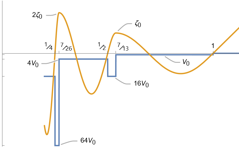
Consider now another solution, , obtained with initial values and . At , will be at zero value with velocity . Then, after the opposing work of , will attain a peak value at . Note that, after each block, the peak value of decreases by a factor of , so . Consequently the norm of this solution is finite. Note also that, after each block, the maximum value of decreases by a factor of , so . Since this solution is real, the probability current is automatically zero, concluding the proof that is confining to .
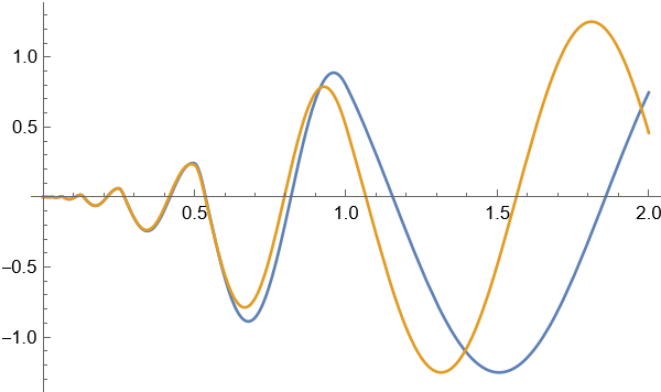
Energy eigenstates. We wish to study the energy eigenstates beyond their asymptotic form. If we start at some point with generic initial conditions, and , and integrate (2) towards , the solution will generally converge to a superposition of and . As is not in the Hilbert space, we wish to restrict the initial conditions so that it converges exclusively to something proportional to .
It is useful to convert (2) to a system of first-order differential equations,
| (9) |
where
| (10) |
The solution, integrating down to , is
| (11) |
with
| (12) |
where denotes the path-ordered exponential (in which greater appears to the right). To obtain a solution behaving like near zero, we must impose that the left-hand side of (11) vanishes in the limit .
However, we cannot simply set above since is ill-defined. Rather, taking , in the limit where the integer , we can impose that the left-hand side of (11) is proportional to , since is precisely defined by having zero derivative at the beginning of each block. The condition is thus,
| (13) |
as goes to infinity. If , the energy can be neglected in the -th block, sitting between and , whose contribution to the path-ordered exponential is therefore
| (14) |
Consequently, as grows large, and will grow as . We can thus properly define the vector
| (15) |
and valid initial data at for an eigenfunction with energy will satisfy
| (16) |
Note that encodes the information about the phase shift in the reflection of a wave packet coming from . For the eigenfunctions have the form
| (17) |
Any wave packet (in the domain of ) can be expanded as a superposition of these eigenfunctions, and their time evolution straightforwardly evaluated.
Spectrum. It is clear that any belongs to the spectrum of the Hamiltonian. In fact, while the eigenfunctions do not have finite norm due to their behavior for , and thus do not belong to the Hilbert space, they can still be used as “generalized basis elements” for the domain of . (footnote 333In particular, for any in the spectrum of , there is a sequence of (normalizable) states such that . Or, in the language of rigged Hilbert spaces [15, 16], these “generalized eigenstates” can be interpreted as antilinear functionals on some dense subspace of the Hilbert space (on which a class of physical observables are all well-defined). Contrastingly, the only linear combinations of “eigenfunctions” behaving like near zero which are in the domain of are those that behave like , justifying why ’s should be disregarded entirely.)
Since the potential is negative, and in fact unbounded from below, it is not surprising that there are also negative energies. The negative portion of the spectrum is, however, discrete. The reason is that the (negative energy) solutions given in (17) will generally consist of one diverging and one converging exponential for , and only the latter is allowed. We need some “fine-tuning” of so that, starting from , the solution of (2) converges to as and to for . The condition is thus that , which from (16) corresponds to
| (18) |
Many interesting properties about the negative spectrum can be studied analytically. First, note that by defining a dimensionless position variable , we can rewrite equation (2) as
| (19) |
where , and
| (20) |
In this new form, the equation is completely dimensionless and, due to relation (5), is independent of the physical parameters (i.e., , and ), implying that the spectrum in terms of is completely invariant. From a numerical computation we find that the first few elements of the (negative part of the) spectrum are
| (21) |
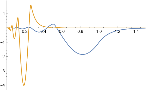
Let us show that if is large and belongs to the spectrum of , then there is another eigenvalue very close to . First, note that for large negative the eigenfunction is concentrated deeply inside the cliff, near , as expected for bound states (see figure 3). So the wavefunction would barely “feel” if the first block of the potential were deleted. Consequently, if is an eigenvalue for a cliff with edge at , then there should exist an eigenvalue for a cliff with edge at . It follows that belongs to the invariant spectrum, and consequently is in the spectrum for a cliff with edge at .
This argument can be formalized using perturbation theory, in which we express the Hamiltonian for a cliff with edge at as , with
| (22) |
where was defined in figure 1. We can estimate, to first order, the effect of on eigenvalues and eigenvectors. For , where is the point at which , the (normalized) eigenfunction behaves roughly like an exponential,
| (23) |
When , we have , , and we can show that
| (24) |
confirming that is indeed very close to . Moreover, the size of the eigenfunction perturbation is bounded by, roughly,
| (25) |
which is again very small for large negative .
A consequence of this is that for any large in the spectrum, can be divided by repeatedly until eventually it will come very close to one of the values in (21). In fact, the agreement is already good from the fourth root, . A similar argument also holds in the other direction, i.e., if is a large negative eigenvalue, then there is another eigenvalue near (which is derived by inserting a “zeroth block” in between and ). It follows that the first few eigenvalues (given in (21)) determine all others, and that the spectrum is unbounded from below.
Conclusion. We have constructed a potential that is well-defined everywhere on and, despite diverging to as , effectively prevents the particle from escaping through . It should be noted that there are simpler, known examples of negative potentials that, in a limit where they diverge, become “opaque” to particles [13, 14]. For example, if for and for , the transmission coefficient for a wave packet coming from the right, computed at , goes to zero in the limit . Another example is a square well where for , and zero elsewhere, which also becomes opaque when provided , with . In either of these cases, the potential does not converge to a limiting function (or even distribution), so the Schrödinger equation is not well-defined after the limit is taken. Moreover, the confining mechanism is taking place beyond the region accessible to the particle, i.e., it is caused by the effect of the potential on . In fact, we can think of our potential as a series of such square wells, where with , in a way that the desired limit is implemented dynamically. This is a crucial distinction, as in our case the particle evolves regularly on and, as it “bungees back” when falling over the cliff, it never reaches “the bottom”, (where is ill-defined), or the “other side”, (where is not-defined).
While we have treated the theory as if it were describing a particle intrinsically living on the half-line, the fact that both and converge to zero at means that the theory on can be regularly embedded into a theory on . That is, can be extended to a wavefunction which agrees with for and vanishes for . If is an extension of to , where is defined arbitrarily for , then any in the domain of is also in the domain of . If not for the regularity condition at , there would be subtle differences between the theory intrinsically on and its extension to . Namely, some would be extended to a that has a discontinuity and/or kink at and, because of the second derivative in the Hamiltonian, it would not be in . As mentioned, this issue does not occur in the present case, for the potential dynamically forces the appropriate boundary conditions.
Acknowledgements. I especially thank Ted Jacobson for valuable discussions and insights, and providing extensive feedback on the draft of this paper. I thank also Pranav Pulakkat, Fritz Gesztesy and Gerald Teschl for useful conversations. This research was supported by the National Science Foundation under Grant PHY-2309634.
References
- Vilenkin [1994] A. Vilenkin, Approaches to quantum cosmology, Physical Review D 50, 2581–2594 (1994).
- Pinto-Neto and Fabris [2013] N. Pinto-Neto and J. Fabris, Quantum cosmology from the de Broglie-Bohm perspective, Classical and Quantum Gravity 30, 143001 (2013).
- Pinto-Neto et al. [2012] N. Pinto-Neto, F. Falciano, R. Pereira, and E. S. Santini, Wheeler-DeWitt quantization can solve the singularity problem, Physical Review D 86, 063504 (2012).
- Kim [1997] S. P. Kim, Quantum potential and cosmological singularities, Physics Letters A 236, 11–15 (1997).
- Harlow and Jafferis [2020] D. Harlow and D. Jafferis, The factorization problem in Jackiw-Teitelboim gravity, Journal of High Energy Physics 2020, 1 (2020).
- Hall [2013] B. C. Hall, Quantum theory for mathematicians (Springer, 2013).
- Reed and Simon [1975] M. Reed and B. Simon, II: Fourier analysis, self-adjointness, Vol. 2 (Elsevier, 1975).
- Weyl [1910] H. Weyl, Über gewöhnliche differentialgleichungen mit singularitäten und die zugehörigen entwicklungen willkürlicher funktionen. (mit 1 figur im text), Mathematische Annalen 68, 220 (1910).
- Zettl [2005] A. Zettl, Sturm-liouville theory, 121 (American Mathematical Soc., 2005).
- Note [1] We say that a function has finite near-zero norm if for some ; and infinite near-zero norm otherwise.
- Note [2] Note that if (3) had two independent solutions with finite near-zero norm, then as the equation is real one could choose a basis of real solutions and , both with finite near-zero norm, and consequently , where is the Wronskian, so that the probability flux is non-zero for generic solutions.
- Note [3] In particular, for any in the spectrum of , there is a sequence of (normalizable) states such that . Or, in the language of rigged Hilbert spaces [15, 16], these “generalized eigenstates” can be interpreted as antilinear functionals on some dense subspace of the Hilbert space (on which a class of physical observables are all well-defined). Contrastingly, the only linear combinations of “eigenfunctions” behaving like near zero which are in the domain of are those that behave like , justifying why ’s should be disregarded entirely.
- Messiah [2014] A. Messiah, Quantum mechanics (Courier Corporation, 2014).
- Wiss [2007] J. Wiss, Quantum tunneling (lecture notes), https://courses.physics.illinois.edu/phys485/fa2015/web/tunneling.pdf (2007), accessed: 2024-05-21.
- De la Madrid [2005] R. De la Madrid, The role of the rigged Hilbert space in quantum mechanics, European journal of physics 26, 287 (2005).
- Gelfand and Vilenkin [1964] I. Gelfand and N. Vilenkin, Generalized Functions, Applications of Hamonic Analysis, IV (1964).