Spin entanglement in two-proton emission from ⁶Be

Abstract

This paper presents an evaluation of coupled-spin entanglement in the two-proton ($2p$) radioactive emission. The three-body model of ⁶Be with the proton-proton interaction, which is adjusted to reproduce the experimental energy release, is utilized. Time-dependent calculation is performed to compute the coupled-spin state of the emitted two protons. The spin-correlation function $S$ as Clauser-Horne-Shimony-Holt (CHSH) indicator is obtained as $\left|S\right|\cong 2.72$. Namely, the $2p$-spin entanglement beyond the limit of local-hidden-variable (LHV) theory is concluded. This entanglement is sensitive to the proton-proton interaction. The short-lived (broad-width) $2p$ state has the weaker spin entanglement. In parallel, the core-proton interactions do not harm this entanglement during the time-dependent decaying process. The CHSH measurement can be a probe into the effective nuclear interaction inside finite systems.

Introduction - Clauser-Horne-Shimony-Holt (CHSH) inequality is one essential property of the quantum-entangled state Clauser et al. (1969). This is one variant of Bell inequality introduced by John Clauser et. al. for the proof of Bell theorem, which claims that certain consequence of quantum mechanics cannot be reproduced by the local-hidden-variable (LHV) theory Bell (1964, 2004). By using the CHSH indicator $S$, the limit of LHV theory is symbolically given as $\left|S\right|\leq 2$. Throughout the history of Bell-CHSH examinations Clauser and Shimony (1978); Aspect et al. (1982); Weihs et al. (1998); Pan et al. (2000); Rowe et al. (2001); Scheidl et al. (2010); Giustina et al. (2015); Shalm et al. (2015); Vasilyev et al. (2017); Storz et al. (2023), the violation of LHV-theory limit has been confirmed. In these examinations, the entangled states of photons, electrons, and atoms are populated and measured to satisfy $\left|S\right|>2$. I emphasize that, for this purpose, many efforts have been devoted to close the loopholes, including those of detection Rowe et al. (2001); Giustina et al. (2015); Shalm et al. (2015), locality Aspect et al. (1982); Weihs et al. (1998); Scheidl et al. (2010), and memory Barrett et al. (2002).

In the nuclear physics, the quantum entanglement plays a role in various scenes Lamehi-Rachti and Mittig (1976); Sakai et al. (2006); Kanada-En’yo (2015); Bulgac (2023); Pazy (2023); Gu et al. (2023); Hengstenberg et al. (2023); Pérez-Obiol et al. (2023); Kou et al. (2024); Kirchner et al. (2024); Robin et al. (2021); Kruppa et al. (2021); Miller (2023a, b); Tichai et al. (2023); Sun et al. (2023). In Ref. Lamehi-Rachti and Mittig (1976) by Lamehi-Rachti and Mittig, the low-energy proton-proton scattering was measured for testing the Bell inequality. In this pioneer work, some extra assumptions were required to certify the violation of LHV-theory limit. In Ref. Sakai et al. (2006), Sakai et. al. performed a novel measurement to demonstrate that a strong entanglement is realized between two protons. This experiment measures the spin-singlet two protons made in the reaction of ²H+$p\longrightarrow^{2}$He+$n$. The spin-correlation function as the CHSH indicator is deduced as $S_{\rm expt}=2.83\pm 0.24_{\rm stat}\pm 0.07_{\rm sys}$, which is in agreement with the non-local quantum mechanics and beyond the LHV-theory limit. Recently, several theoretical works have been devoted to compute the entanglement entropy in atomic nuclei Kanada-En’yo (2015); Bulgac (2023); Pazy (2023); Gu et al. (2023); Hengstenberg et al. (2023); Pérez-Obiol et al. (2023); Kou et al. (2024); Kirchner et al. (2024). In Ref. Bulgac (2023), due to the nuclear short-range correlations, the occupation probabilities of nuclear orbits change to increase the entanglement entropy. In Ref. Bai (2024), the evaluation of nuclear spin entanglement with the quantum-state tomography is suggested to be feasible. In Refs. Johnson and Gorton (2023); Miller (2023b), a finite proton-neutron entanglement is suggested.

Another possible example to observe the nuclear quantum entanglement is the two-proton ($2p$) radioactive emission Bertulani et al. (2008); Grigorenko (2009); Pfützner et al. (2012); Blank and Ploszajczak (2008); Blank and Borge (2008); Pfützner et al. (2023); Qi et al. (2019). In this radioactive decay, the parent nuclei spontaneously decay by emitting two protons. Especially in so-called “prompt” $2p$ emission Grigorenko (2009); Goldansky (1960, 1961), the two protons are expected to have the diproton-like clustering and/or the dominant spin-singlet configuration. This is attributable to the effective $2p$ interaction inside finite systems, being in a contrast to the vacuum $2p$ interaction supporting no bound state.

In this paper, I evaluate the quantum entaglement in the $2p$ emission of ⁶Be. Main motivation is to utilize this entanglement as a probe into the effective interaction. The ⁶Be is the lightest $2p$ emitter and well approximated with the simple three-body model with time dependence Oishi et al. (2014, 2017); Wang and Nazarewicz (2021). For the two protons spontaneously emitted, the measurement of their coupled-spin correlation is assumed Bertulani et al. (2008). For quantitizing the entanglement, the CHSH indicator $S$, which was originally introduced for testing the CHSH inequality Clauser et al. (1969); Sakai et al. (2006), is computed. Because of the three-body problem, the $2p$ entanglement is under the effect from the third particle, namely, the daughter alpha nucleus. Whether this effect destroys or not the entanglement is investigated. The sensitivity of CHSH indicator to the proton-proton interaction is also discussed.

Formalism and Model - I consider the coupling of two protons, i.e., identical spin-$1/2$ fermions. In such a case, the CHSH indicator is represented as follows. First the four options of measurement by the two observers, so-called “Alice” and “Bob” by convenance, are introduced:

$$\hat{A}_{1,\theta}(1)\otimes\hat{B}_{1,\theta}(2),~{}\hat{A}_{2,\theta}(1)\otimes\hat{B}_{1,\theta}(2),$$

$$\hat{A}_{1,\theta}(1)\otimes\hat{B}_{2,\theta}(2),~{}\hat{A}_{2,\theta}(1)\otimes\hat{B}_{2,\theta}(2),$$ (1)

Namely, Alice observes the first fermion with one choosen from the two options, $\hat{A}_{1,\theta}$ and $\hat{A}_{2,\theta}$. Bob does the second fermion with one choosen from $\hat{B}_{1,\theta}$ and $\hat{B}_{2,\theta}$. Those operators including the parameter angle $\theta$ are given as

$$\hat{A}_{1}=\hat{\sigma}_{z},~{}~{}~{}~{}\hat{A}_{2,\theta}=\hat{\sigma}_{z}\cos 2\theta+\hat{\sigma}_{x}\sin 2\theta,$$ (2)

for Alice, whereas

$$\begin{array}[]{l}\hat{B}_{1,\theta}=\hat{\sigma}_{z}\cos\theta+\hat{\sigma}_{x}\sin\theta,\\ \hat{B}_{2,\theta}=\hat{\sigma}_{z}\cos\theta-\hat{\sigma}_{x}\sin\theta,\end{array}$$ (3)

for Bob. For an arbitrary two-fermion state $\ket{\Psi(1,2)}$, their expectation values are obtained:

$$\Braket{A_{i}B_{j}}=\Braket{\Psi(1,2)\mid\hat{A}_{i,\theta}(1)\otimes\hat{B}_{j,\theta}(2)\mid\Psi(1,2)}.$$ (4)

Then the CHSH indicator $S$ is determined as

$$S=\max\left\{\left|S_{-+++}\right|,\left|S_{+-++}\right|,\left|S_{++-+}\right|,\left|S_{+++-}\right|\right\},$$ (5)

where

$$S_{-+++} = -\Braket{A_{1}B_{1}}+\Braket{A_{2}B_{1}}+\Braket{A_{1}B_{2}}+\Braket{A_{2}B_{2}},$$

$$S_{+-++} = \Braket{A_{1}B_{1}}-\Braket{A_{2}B_{1}}+\Braket{A_{1}B_{2}}+\Braket{A_{2}B_{2}},$$

$$S_{++-+} = \Braket{A_{1}B_{1}}+\Braket{A_{2}B_{1}}-\Braket{A_{1}B_{2}}+\Braket{A_{2}B_{2}},$$

$$S_{+++-} = \Braket{A_{1}B_{1}}+\Braket{A_{2}B_{1}}+\Braket{A_{1}B_{2}}-\Braket{A_{2}B_{2}}.$$ (6)

In FIG. 1, the CHSH indicator for the spin-singlet state, $\ket{\Psi(1,2)}=\ket{\uparrow\downarrow-\downarrow\uparrow}/\sqrt{2}$, is presented. At $\theta=\pi/4,~{}3\pi/4,~{}5\pi/4$, and $7\pi/4$, this indicator has the maximum value, $S=2\sqrt{2}$ (Tsirelson’s bound) Cirel’son (1980). This situation resembles Sakai’s experiment Sakai et al. (2006). In the following sections, $\theta=\pi/4$, except when modified.

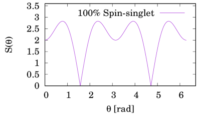
FIG. 1: CHSH indicator of the pure spin-singlet state.

As well known, when the initial state is one of the Bell states, $\ket{\Psi(1,2)}=\ket{e_{n}}$, the CHSH indicator satisfies $S=2\sqrt{2}$ when $\theta=\pi/4$. Here the Bell states read Nielsen and Chuang (2000)

$$\ket{e_{1}}=\frac{1}{\sqrt{2}}\ket{\uparrow\uparrow+\downarrow\downarrow},~{}~{}~{}~{}~{}\ket{e_{2}}=\frac{i}{\sqrt{2}}\ket{\uparrow\uparrow-\downarrow\downarrow},$$

$$\ket{e_{3}}=\frac{i}{\sqrt{2}}\ket{\uparrow\downarrow+\downarrow\uparrow},~{}~{}~{}~{}~{}\ket{e_{4}}=\frac{1}{\sqrt{2}}\ket{\uparrow\downarrow-\downarrow\uparrow}.$$ (7)

These states can be used as basis to represent an arbitrary coupling of two spin-$1/2$ fermions. In addition, there can be also coordinate degrees of freedom. Thus, an arbitrary two-fermion state is generally expanded as

$$\ket{\Psi(1,2)}=\sum_{i=1}^{4}G_{i}(\bm{r}_{1},\bm{r}_{2})\ket{e_{i}},$$ (8)

where $G_{i}(\bm{r}_{1},\bm{r}_{2})$ is the coordinate part.

For the coupled spin $\hat{S}_{12}$, its eigenvalues are given as $\hat{S}^{2}_{12}\ket{d_{k}}=S(S+1)\ket{d_{k}}$ and $\hat{S}_{12,z}\ket{d_{k}}=V\ket{d_{k}}$, where

$$\ket{d_{1}} = \ket{S=1,V=+1}=\ket{\uparrow\uparrow},$$

$$\ket{d_{2}} = \ket{S=1,V=-1}=\ket{\downarrow\downarrow},$$

$$\ket{d_{3}} = \ket{S=1,V=0}=\frac{1}{\sqrt{2}}\ket{\uparrow\downarrow+\downarrow\uparrow},$$

$$\ket{d_{4}} = \ket{S=0,V=0}=\frac{1}{\sqrt{2}}\ket{\uparrow\downarrow-\downarrow\uparrow}.$$ (9)

Then, the unitary transformation $U$ is formulated:

$$\begin{array}[]{l}\ket{e_{1}}\\ \ket{e_{2}}\\ \ket{e_{3}}\\ \ket{e_{4}}\end{array}=U\begin{array}[]{l}\ket{d_{1}}\\ \ket{d_{2}}\\ \ket{d_{3}}\\ \ket{d_{4}}\end{array}=\left(\begin{array}[]{llll}\frac{1}{\sqrt{2}}&\frac{1}{\sqrt{2}}&0&0\\ \frac{i}{\sqrt{2}}&\frac{-i}{\sqrt{2}}&0&0\\ 0&0&i&0\\ 0&0&0&1\end{array}\right)\begin{array}[]{l}\ket{d_{1}}\\ \ket{d_{2}}\\ \ket{d_{3}}\\ \ket{d_{4}}\end{array}.$$ (10)

In the following sections, the total-spin basis is also utilized: $\ket{\Psi(1,2)}=\sum_{i}F_{i}(\bm{r}_{1},\bm{r}_{2})\ket{d_{i}}$. Thus, $G_{i}(\bm{r}_{1},\bm{r}_{2})=\sum_{k}\left(U^{\dagger}\right)_{ik}F_{k}(\bm{r}_{1},\bm{r}_{2})$ to convert to Bell basis. Notice that, for computing the expectation values in Eq. (6), these coordinate parts can be simply integrated.

I employ the three-body model, which has been developed and utilized in Refs. Suzuki and Ikeda (1988); Bertsch and Esbensen (1991); Esbensen et al. (1997); Hagino and Sagawa (2005); Oishi et al. (2014, 2017). The system contains an alpha particle as the rigid core with mass $m_{C}$ and two valence protons. The two valence protons feel the spherical mean field $V(\bm{r})$ generated by the alpha core. Thus, the three-body Hamiltonian reads

$$\hat{H}_{3B}=\hat{h}(\bm{r}_{1})+\hat{h}(\bm{r}_{2})+v_{pp}(\bm{r}_{1},\bm{r}_{2})+\frac{\bm{p}_{1}\cdot\bm{p}_{2}}{m_{C}},$$ (11)

$$\hat{h}(r_{i})=-\frac{\hbar^{2}}{2\mu}\frac{d^{2}}{dr_{i}^{2}}+\frac{\hbar^{2}}{2\mu}\frac{l(l+1)}{r_{i}^{2}}+V(r_{i}),$$ (12)

where $\mu=m_{p}m_{C}/(m_{p}+m_{C})$ and $m_{p}=938.272$ MeV$/c^{2}$ for protons. Here $\hat{h}(\bm{r}_{k})$ is of the $k$th proton-alpha subsystem. For its interaction $V(r_{i})$, the same Woods-Saxon and Coulomb potentials in the previous work Oishi et al. (2017) are employed. The proton-proton interaction reads

$$v_{pp}(\bm{r}_{1},\bm{r}_{2})=v_{nucl}(d)+\frac{e^{2}}{4\pi\epsilon_{0}}\frac{1}{d}+v_{add}(\bm{r}_{1},\bm{r}_{2}),$$ (13)

where $d=\left|\bm{r}_{2}-\bm{r}_{1}\right|$. The nuclear-force term is described by the spin-dependent Gaussian potential Thompson et al. (1977):

$$v_{nucl}(d) = \left[V_{R}e^{-a_{R}d^{2}}+V_{S}e^{-a_{S}d^{2}}\right]\hat{P}_{S=0}$$ (14)

$$+\left[V_{R}e^{-a_{R}d^{2}}+V_{T}e^{-a_{T}d^{2}}\right]\hat{P}_{S=1}.$$

The operator $\hat{P}_{S=0}$ ($\hat{P}_{S=1}$) indicates the projection into the spin-singlet (spin-triplet) channel of the proton-proton subsystem. Parameters are given as $V_{R}=200$ MeV, $V_{S}=-91.85$ MeV, $V_{T}=-178$ MeV, $a_{R}=1,487$ fm^-2, $a_{S}=0.465$ fm^-2, and $a_{T}=0.639$ fm^-2. These parameters correctly reproduce the experimental vacuum-scattering length of two protons Thompson et al. (1977). In addition, the surface-dependent term $v_{add}$ is employed:

$$v_{add}(\bm{r}_{1},\bm{r}_{2})=w_{0}e^{-(R-R_{0})^{2}/B_{0}^{2}}\delta(\bm{r}_{1}-\bm{r}_{2}),$$ (15)

where $R=\left|(\bm{r}_{1}+\bm{r}_{2})/2\right|$, $R_{0}=1.68$ fm, $B_{0}=0.6R_{0}$, and $w_{0}=-470$ MeV$\cdot$fm³. This additional term is necessary to reproduce the experimental energy: the $2p$ energy and width are obtained as $E_{2p}=1.356$ MeV and $\Gamma_{2p}=0.055$ MeV, respectively, whereas the experimental data read $E_{2p}=1.372(5)$ MeV and $\Gamma_{2p}=0.092(6)$ MeV Ajzenberg-Selove (1988, 1991). Notice that this additional potential vanishes when one of the three particles is infinitely separated. Thus, the vacuum properties of two-body subsystems can be conserved in the time-development calculations. I especially notify that the emitted two protons should be unbound in vacuum.

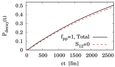
FIG. 2: Time-dependent decaying probability of $2p$ emission from ⁶Be. Its spin-singlet ($S_{12}=0$) component is also plotted. The factor $f_{pp}=1$ indicates that the proton-proton interaction is adjusted to reproduce the experimental $2p$-energy.

Results and Discussions - The $2p$-emitting process is simulated with the time-dependent method Oishi et al. (2014, 2017):

$$\ket{\Psi(t)}=\exp\left[-it\frac{\hat{H}_{3B}}{\hbar}\right]\ket{\Psi(0)},$$ (16)

where the initial state is solved as the confined $2p$ state inside the Coulomb barrier Oishi et al. (2014). The decaying state $\ket{\Psi_{d}(t)}$, which describes the emitted component outside the barrier, is determined as

$$\ket{\Psi_{d}(t)}=\ket{\Psi(t)}-\beta(t)\ket{\Psi(0)},$$ (17)

where $\beta(t)$ is the survival coefficient, $\beta(t)=\Braket{\Psi(0)}{\Psi(t)}$.

In FIG 2, the time-dependent decaying probability is displayed:

$$P_{decay}(t)=\Braket{\Psi_{d}(t)\mid\Psi_{d}(t)}=1-\left|\beta(t)\right|^{2}.$$ (18)

One clearly finds that the decaying probability increases in time development. The spin-singlet state, $\ket{d_{4}}=\ket{e_{4}}=\ket{\uparrow\downarrow-\downarrow\uparrow}/\sqrt{2}$, is always dominant. I confirmed that the survival probability,

$$P_{surv}(t)\equiv\Braket{\Psi(0)\mid\Psi(t)}^{2}=\left|\beta(t)\right|^{2}=1-P_{decay}(t),$$ (19)

is well approximated by the exponential damping. Namely, $P_{surv}(t)\cong e^{-t/\tau}$, where the width can be evaluated as $\Gamma_{2p}=\hbar/\tau\cong 0.055$ MeV by numerical fitting. Also, by observing the decaying density distribution, $\rho_{d}(t,\bm{r}_{1},\bm{r}_{2})=\left|\Psi_{d}(t,\bm{r}_{1},\bm{r}_{2})\right|^{2}$, I confirmed that the present $2p$ emission can be interpreted as the diproton-correlating emission Oishi et al. (2014, 2017).

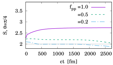
FIG. 3: CHSH indicator of the time-dependent decaying state $\ket{\Psi_{d}(t)}$ of the $2p$ emission of ⁶Be $\longrightarrow\alpha+p+p$. Here $\theta=\pi/4$. The factor $f_{pp}$ indicates the strength of the proton-proton interaction.

In Fig. 3, the CHSH indicator is evaluated for the decaying state by using the expansion,

$$\ket{\Psi_{d}(t,\bm{r}_{1},\bm{r}_{2})}=\sum_{i=1}^{4}G_{i}(t,\bm{r}_{1},\bm{r}_{2}))\ket{e_{i}}.$$ (20)

One clearly finds that the CHSH indicator becomes larger than $2$, i.e. the LHV-theory limit, during the time evolution. For $ct\geq 1500$ fm, I obtain $S\cong 2.72$ with the default setting of $v_{pp}$ ($f_{pp}=1.0$) for reproducing $E_{2p}=1.356$ MeV of ⁶Be Ajzenberg-Selove (1988, 1991). This coupled-spin entanglement is of course attributable to the dominant spin-singlet component in FIG 2.

Notice that the present time evolution in Eq. (16) also contains the effect of core-proton interactions $V(r_{i})$. These interactions do not harm the $2p$ entanglement.

For deeper investigation, the sensitivity of CHSH indicator to the proton-proton interaction is studied. For this purpose, an effective tuning factor is employed:

$$v_{pp}(\bm{r}_{1},\bm{r}_{2})\longrightarrow f_{pp}v_{pp}(\bm{r}_{1},\bm{r}_{2}).$$ (21)

With $f_{pp}=1$, the $v_{pp}$ approximates the experimental energy, $E_{2p}=1.356$ MeV Ajzenberg-Selove (1988, 1991). From FIG. 3, one can read that this CHSH indicator becomes smaller when the interaction is weakened. In the present case of ⁶Be, it goes below the LHV-theory limit, $S<2$, with $f_{pp}\leq 0.2$. Consequently, the present entanglement is a product of the proton-proton interaction. With the $v_{pp}$ weakened, the $2p$ energy and width also change: $E_{2p}=2.864$ MeV and $\Gamma_{2p}=0.8579$ MeV with $f_{pp}=0.5$; $E_{2p}=2.925$ MeV and $\Gamma_{2p}\cong 2.9$ MeV with $f_{pp}=0.2$. Thus, the short-lived (broad-width) $2p$ state has the weaker spin entanglement.

Summary - In this paper, the CHSH indicator for the $2p$ emission from ⁶Be is evaluated in order to measure its coupled-spin entanglement. As a product of proton-proton interaction, $S\cong 2.72$ is obtained in the time-dependent decaying state: an entanglement beyond the limit of LHV theory is suggested. This entanglement is not harmed by the core-proton interactions. The CHSH measurement can be a probe into the effective nuclear interaction inside finite systems.

This work is limited to the lightest ⁶Be nucleus. Whether the spin entanglement exists commonly in other $2p$ emitters or not is an open question. The dominance of spin-singlet Bell state is not trivial in other systems. For evaluating the quantum entanglement, the von-Neumann entropy has been considered as an essential quantity Kanada-En’yo (2015); Bulgac (2023); Pazy (2023); Gu et al. (2023); Hengstenberg et al. (2023); Pérez-Obiol et al. (2023); Kou et al. (2024); Kirchner et al. (2024), whereas this work focuses only on the CHSH indicator. Evaluation and discussion of the von-Neumann entropy for the time-dependent state is in progress. Whether the entanglement is apparent or not may depend on the observable quantity of interest, e.g. the coupled spin, momenta, and energy distribution. These topics will be addressed in forthcoming studies.

In the experimental side, mass production of $2p$ emitters, including the ⁶Be, for a sufficient statistics is still challenging. For measuring the two protons by independent detectors after decay, an advanced design of experiment will be necessary. Closing all the loopholes of detection Rowe et al. (2001); Giustina et al. (2015); Shalm et al. (2015), locality Aspect et al. (1982); Weihs et al. (1998); Scheidl et al. (2010), and memory Barrett et al. (2002) should require another lot of efforts. On the other side, the experimental survey of $2p$ emitters is rapidly in progress, e.g. that in RIKEN RIBF. Confirmation of spin entanglement in $2p$ radioactivity can be one landmark in the nuclear physics as well as quantum many-body science.

Acknowledgments - I especially thank Yutaka Shikano, Masaki Sasano, Tomoya Naito, Tokuro Fukui, and Masaaki Kimura for fruitful discussions. Numerical calculations are supported by the cooperative project of supercomputer Yukawa-21 in Yukawa Institute for Theoretical Physics, Kyoto University. I appreciate the Multi-disciplinary Cooperative Research Program (MCRP) 2023-2024 by Center for Computational Sciences, University of Tsukuba (project ID wo23i034), allocating computational resources of supercomputer Wisteria/BDEC-01 (Odyssey) in Information Technology Center, University of Tokyo.

References

- Clauser et al. (1969) J. F. Clauser, M. A. Horne, A. Shimony, and R. A. Holt, Phys. Rev. Lett. 23, 880 (1969).
- Bell (1964) J. Bell, Physics 1, 195 (1964).
- Bell (2004) J. S. Bell, Speakable and Unspeakable in Quantum Mechanics, 2nd ed., Collected Papers on Quantum Philosophy (Cambridge University Press, Cambridge, UK, 2004).
- Clauser and Shimony (1978) J. F. Clauser and A. Shimony, Reports on Progress in Physics 41, 1881 (1978).
- Aspect et al. (1982) A. Aspect, P. Grangier, and G. Roger, Phys. Rev. Lett. 49, 91 (1982).
- Weihs et al. (1998) G. Weihs, T. Jennewein, C. Simon, H. Weinfurter, and A. Zeilinger, Phys. Rev. Lett. 81, 5039 (1998).
- Pan et al. (2000) J.-W. Pan, D. Bouwmeester, M. Daniell, H. Weinfurter, and A. Zeilinger, Nature 403, 515 (2000).
- Rowe et al. (2001) M. A. Rowe, D. Kielpinski, V. Meyer, C. A. Sackett, W. M. Itano, C. Monroe, and D. J. Wineland, Nature 409, 791 (2001).
- Scheidl et al. (2010) T. Scheidl, R. Ursin, J. Kofler, S. Ramelow, X.-S. Ma, T. Herbst, L. Ratschbacher, A. Fedrizzi, N. K. Langford, T. Jennewein, and A. Zeilinger, Proceedings of the National Academy of Sciences 107, 19708 (2010), https://www.pnas.org/doi/pdf/10.1073/pnas.1002780107 .
- Giustina et al. (2015) M. Giustina, M. A. M. Versteegh, S. Wengerowsky, J. Handsteiner, A. Hochrainer, K. Phelan, F. Steinlechner, J. Kofler, J.-A. Larsson, C. Abellán, W. Amaya, V. Pruneri, M. W. Mitchell, J. Beyer, T. Gerrits, A. E. Lita, L. K. Shalm, S. W. Nam, T. Scheidl, R. Ursin, B. Wittmann, and A. Zeilinger, Phys. Rev. Lett. 115, 250401 (2015).
- Shalm et al. (2015) L. K. Shalm, E. Meyer-Scott, B. G. Christensen, P. Bierhorst, M. A. Wayne, M. J. Stevens, T. Gerrits, S. Glancy, D. R. Hamel, M. S. Allman, K. J. Coakley, S. D. Dyer, C. Hodge, A. E. Lita, V. B. Verma, C. Lambrocco, E. Tortorici, A. L. Migdall, Y. Zhang, D. R. Kumor, W. H. Farr, F. Marsili, M. D. Shaw, J. A. Stern, C. Abellán, W. Amaya, V. Pruneri, T. Jennewein, M. W. Mitchell, P. G. Kwiat, J. C. Bienfang, R. P. Mirin, E. Knill, and S. W. Nam, Phys. Rev. Lett. 115, 250402 (2015).
- Vasilyev et al. (2017) D. Vasilyev, F. O. Schumann, F. Giebels, H. Gollisch, J. Kirschner, and R. Feder, Phys. Rev. B 95, 115134 (2017).
- Storz et al. (2023) S. Storz, J. Schär, A. Kulikov, P. Magnard, P. Kurpiers, J. Lütolf, T. Walter, A. Copetudo, K. Reuer, A. Akin, J.-C. Besse, M. Gabureac, G. J. Norris, A. Rosario, F. Martin, J. Martinez, W. Amaya, M. W. Mitchell, C. Abellan, J.-D. Bancal, N. Sangouard, B. Royer, A. Blais, and A. Wallraff, Nature 617, 265 (2023).
- Barrett et al. (2002) J. Barrett, D. Collins, L. Hardy, A. Kent, and S. Popescu, Phys. Rev. A 66, 042111 (2002).
- Lamehi-Rachti and Mittig (1976) M. Lamehi-Rachti and W. Mittig, Phys. Rev. D 14, 2543 (1976).
- Sakai et al. (2006) H. Sakai, T. Saito, T. Ikeda, K. Itoh, T. Kawabata, H. Kuboki, Y. Maeda, N. Matsui, C. Rangacharyulu, M. Sasano, Y. Satou, K. Sekiguchi, K. Suda, A. Tamii, T. Uesaka, and K. Yako, Phys. Rev. Lett. 97, 150405 (2006).
- Kanada-En’yo (2015) Y. Kanada-En’yo, Progress of Theoretical and Experimental Physics 2015, 043D04 (2015).
- Bulgac (2023) A. Bulgac, Phys. Rev. C 107, L061602 (2023).
- Pazy (2023) E. Pazy, Phys. Rev. C 107, 054308 (2023).
- Gu et al. (2023) C. Gu, Z. H. Sun, G. Hagen, and T. Papenbrock, Phys. Rev. C 108, 054309 (2023).
- Hengstenberg et al. (2023) S. M. Hengstenberg, C. E. P. Robin, and M. J. Savage, The European Physical Journal A 59, 231 (2023).
- Pérez-Obiol et al. (2023) A. Pérez-Obiol, S. Masot-Llima, A. M. Romero, J. Menéndez, A. Rios, A. Garcia-Sáez, and B. Juliá-Diaz, The European Physical Journal A 59, 240 (2023).
- Kou et al. (2024) W. Kou, J. Chen, and X. Chen, Physics Letters B 849, 138453 (2024).
- Kirchner et al. (2024) T. Kirchner, W. Elkamhawy, and H.-W. Hammer, Few-Body Systems 65, 29 (2024).
- Robin et al. (2021) C. Robin, M. J. Savage, and N. Pillet, Phys. Rev. C 103, 034325 (2021).
- Kruppa et al. (2021) A. T. Kruppa, J. Kovács, P. Salamon, and O. Legeza, Journal of Physics G: Nuclear and Particle Physics 48, 025107 (2021).
- Miller (2023a) G. A. Miller, Phys. Rev. C 108, L041601 (2023a).
- Miller (2023b) G. A. Miller, Phys. Rev. C 108, L031002 (2023b).
- Tichai et al. (2023) A. Tichai, S. Knecht, A. Kruppa, O. Legeza, C. Moca, A. Schwenk, M. Werner, and G. Zarand, Physics Letters B 845, 138139 (2023).
- Sun et al. (2023) Z. H. Sun, G. Hagen, and T. Papenbrock, Phys. Rev. C 108, 014307 (2023).
- Bai (2024) D. Bai, Phys. Rev. C 109, 034001 (2024).
- Johnson and Gorton (2023) C. W. Johnson and O. C. Gorton, Journal of Physics G: Nuclear and Particle Physics 50, 045110 (2023).
- Bertulani et al. (2008) C. Bertulani, M. Hussein, and G. Verde, Physics Letters B 666, 86 (2008).
- Grigorenko (2009) L. V. Grigorenko, Physics of Particles and Nuclei 40, 674 (2009).
- Pfützner et al. (2012) M. Pfützner, M. Karny, L. V. Grigorenko, and K. Riisager, Rev. Mod. Phys. 84, 567 (2012).
- Blank and Ploszajczak (2008) B. Blank and M. Ploszajczak, Reports on Progress in Physics 71, 046301 (2008).
- Blank and Borge (2008) B. Blank and M. Borge, Progress in Particle and Nuclear Physics 60, 403 (2008).
- Pfützner et al. (2023) M. Pfützner, I. Mukha, and S. Wang, Progress in Particle and Nuclear Physics 132, 104050 (2023).
- Qi et al. (2019) C. Qi, R. Liotta, and R. Wyss, Progress in Particle and Nuclear Physics 105, 214 (2019).
- Goldansky (1960) V. I. Goldansky, Nucl. Phys. 19, 482 (1960).
- Goldansky (1961) V. I. Goldansky, Nucl. Phys. 27, 648 (1961).
- Oishi et al. (2014) T. Oishi, K. Hagino, and H. Sagawa, Phys. Rev. C 90, 034303 (2014).
- Oishi et al. (2017) T. Oishi, M. Kortelainen, and A. Pastore, Phys. Rev. C 96, 044327 (2017).
- Wang and Nazarewicz (2021) S. M. Wang and W. Nazarewicz, Phys. Rev. Lett. 126, 142501 (2021).
- Cirel’son (1980) B. S. Cirel’son, Letters in Mathematical Physics 4, 93 (1980).
- Nielsen and Chuang (2000) M. Nielsen and I. Chuang, Quantum Computation and Quantum Information (Cambridge University Press, Cambridge, UK, 2000).
- Suzuki and Ikeda (1988) Y. Suzuki and K. Ikeda, Phys. Rev. C 38, 410 (1988).
- Bertsch and Esbensen (1991) G. Bertsch and H. Esbensen, Annals of Physics 209, 327 (1991).
- Esbensen et al. (1997) H. Esbensen, G. F. Bertsch, and K. Hencken, Phys. Rev. C 56, 3054 (1997).
- Hagino and Sagawa (2005) K. Hagino and H. Sagawa, Phys. Rev. C 72, 044321 (2005).
- Thompson et al. (1977) D. Thompson, M. Lemere, and Y. Tang, Nuclear Physics A 286, 53 (1977).
- Ajzenberg-Selove (1988) F. Ajzenberg-Selove, Nuclear Physics A 490, 1 (1988), note: several versions with the same title has been published.
- Ajzenberg-Selove (1991) F. Ajzenberg-Selove, Nuclear Physics A 523, 1 (1991), with revised version at http://www.tunl.duke.edu/nucldata/.